Systematic Topology Analysis and GenerationUsing Degree Correlations

Priya MahadevanUC San Diego

Dmitri KrioukovCAIDA

Kevin FallIntel Research

Amin VahdatUC San Diego

{pmahadevan,vahdat}@cs.ucsd.edu, dima@caida.org, kevin.fall@intel.com

ABSTRACTResearchers have proposed a variety of metrics to measureimportant graph properties, for instance, in social, biologi-cal, and computer networks. Values for a particular graphmetric may capture a graph’s resilience to failure or its rout-ing efficiency. Knowledge of appropriate metric values mayinfluence the engineering of future topologies, repair strate-gies in the face of failure, and understanding of fundamen-tal properties of existing networks. Unfortunately, there aretypically no algorithms to generate graphs matching one ormore proposed metrics and there is little understanding ofthe relationships among individual metrics or their applica-bility to different settings.

We present a new, systematic approach for analyzing net-work topologies. We first introduce the dK-series of proba-bility distributions specifying all degree correlations withind-sized subgraphs of a given graph G. Increasing values ofd capture progressively more properties of G at the costof more complex representation of the probability distribu-tion. Using this series, we can quantitatively measure thedistance between two graphs and construct random graphsthat accurately reproduce virtually all metrics proposed inthe literature. The nature of the dK-series implies that itwill also capture any future metrics that may be proposed.Using our approach, we construct graphs for d = 0, 1, 2, 3and demonstrate that these graphs reproduce, with increas-ing accuracy, important properties of measured and modeledInternet topologies. We find that the d = 2 case is sufficientfor most practical purposes, while d = 3 essentially recon-structs the Internet AS- and router-level topologies exactly.We hope that a systematic method to analyze and synthe-size topologies offers a significant improvement to the set oftools available to network topology and protocol researchers.

Categories and Subject DescriptorsC.2.1 [Network Architecture and Design]: Networktopology; G.3 [Probability and Statistics]: Distributionfunctions, multivariate statistics, correlation and regression

Permission to make digital or hard copies of all or part of this work forpersonal or classroom use is granted without fee provided that copies arenot made or distributed for profit or commercial advantage and that copiesbear this notice and the full citation on the first page. To copy otherwise, torepublish, to post on servers or to redistribute to lists, requires prior specificpermission and/or a fee.SIGCOMM’06, September 11–15, 2006, Pisa, Italy.Copyright 2006 ACM 1-59593-308-5/06/0009 ...$5.00.

Measurements, observations

Observed graphsSelection and abstraction

Graph metricsto reproduce

Network evolution modeling

Synthetic ‘growing’ graphs

Synthetic‘static’ graphs

Simulations

Comparison with the observed graphs against a set of

important graph properties

Topology Processes

Extraction

Construction Execution

Formalization

If graphs differ, refinements are needed:modify the set of

reproduced graph metrics (on the left)or abstracted evolution rules (on the right)

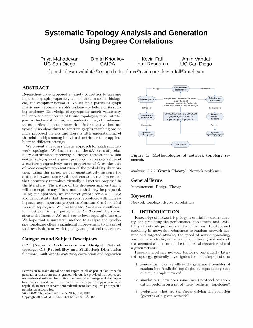
Figure 1: Methodologies of network topology re-

search.

analysis; G.2.2 [Graph Theory]: Network problems

General TermsMeasurement, Design, Theory

KeywordsNetwork topology, degree correlations

1. INTRODUCTIONKnowledge of network topology is crucial for understand-

ing and predicting the performance, robustness, and scala-bility of network protocols and applications. Routing andsearching in networks, robustness to random network fail-ures and targeted attacks, the speed of worms spreading,and common strategies for traffic engineering and networkmanagement all depend on the topological characteristics ofa given network.

Research involving network topology, particularly Inter-net topology, generally investigates the following questions:

1. generation: can we efficiently generate ensembles ofrandom but “realistic” topologies by reproducing a setof simple graph metrics?

2. simulations: how does some (new) protocol or appli-cation perform on a set of these “realistic” topologies?

3. evolution: what are the forces driving the evolution(growth) of a given network?

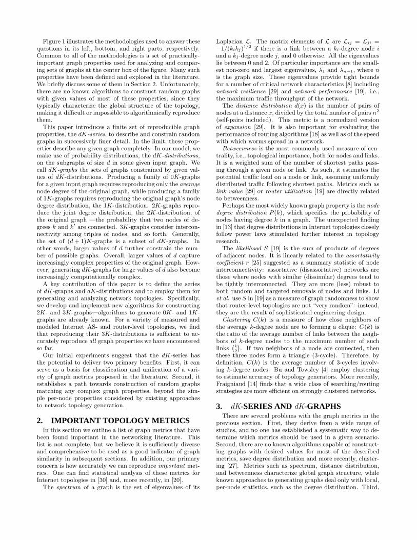
Figure 1 illustrates the methodologies used to answer thesequestions in its left, bottom, and right parts, respectively.Common to all of the methodologies is a set of practically-important graph properties used for analyzing and compar-ing sets of graphs at the center box of the figure. Many suchproperties have been defined and explored in the literature.We briefly discuss some of them in Section 2. Unfortunately,there are no known algorithms to construct random graphswith given values of most of these properties, since theytypically characterize the global structure of the topology,making it difficult or impossible to algorithmically reproducethem.

This paper introduces a finite set of reproducible graphproperties, the dK-series, to describe and constrain randomgraphs in successively finer detail. In the limit, these prop-erties describe any given graph completely. In our model, wemake use of probability distributions, the dK-distributions,on the subgraphs of size d in some given input graph. Wecall dK-graphs the sets of graphs constrained by given val-ues of dK-distributions. Producing a family of 0K-graphsfor a given input graph requires reproducing only the average

node degree of the original graph, while producing a familyof 1K-graphs requires reproducing the original graph’s nodedegree distribution, the 1K-distribution. 2K-graphs repro-duce the joint degree distribution, the 2K-distribution, ofthe original graph —the probability that two nodes of de-grees k and k′ are connected. 3K-graphs consider intercon-nectivity among triples of nodes, and so forth. Generally,the set of (d + 1)K-graphs is a subset of dK-graphs. Inother words, larger values of d further constrain the num-ber of possible graphs. Overall, larger values of d captureincreasingly complex properties of the original graph. How-ever, generating dK-graphs for large values of d also becomeincreasingly computationally complex.

A key contribution of this paper is to define the seriesof dK-graphs and dK-distributions and to employ them forgenerating and analyzing network topologies. Specifically,we develop and implement new algorithms for constructing2K- and 3K-graphs—algorithms to generate 0K- and 1K-graphs are already known. For a variety of measured andmodeled Internet AS- and router-level topologies, we findthat reproducing their 3K-distributions is sufficient to ac-curately reproduce all graph properties we have encounteredso far.

Our initial experiments suggest that the dK-series hasthe potential to deliver two primary benefits. First, it canserve as a basis for classification and unification of a vari-ety of graph metrics proposed in the literature. Second, itestablishes a path towards construction of random graphsmatching any complex graph properties, beyond the sim-ple per-node properties considered by existing approachesto network topology generation.

2. IMPORTANT TOPOLOGY METRICSIn this section we outline a list of graph metrics that have

been found important in the networking literature. Thislist is not complete, but we believe it is sufficiently diverseand comprehensive to be used as a good indicator of graphsimilarity in subsequent sections. In addition, our primaryconcern is how accurately we can reproduce important met-rics. One can find statistical analysis of these metrics forInternet topologies in [30] and, more recently, in [20].

The spectrum of a graph is the set of eigenvalues of its

Laplacian L. The matrix elements of L are Lij = Lji =−1/(kikj)

1/2 if there is a link between a ki-degree node iand a kj-degree node j, and 0 otherwise. All the eigenvalueslie between 0 and 2. Of particular importance are the small-est non-zero and largest eigenvalues, λ1 and λn−1, where nis the graph size. These eigenvalues provide tight boundsfor a number of critical network characteristics [8] includingnetwork resilience [29] and network performance [19], i.e.,the maximum traffic throughput of the network.

The distance distribution d(x) is the number of pairs ofnodes at a distance x, divided by the total number of pairs n2

(self-pairs included). This metric is a normalized versionof expansion [29]. It is also important for evaluating theperformance of routing algorithms [18] as well as of the speedwith which worms spread in a network.

Betweenness is the most commonly used measure of cen-trality, i.e., topological importance, both for nodes and links.It is a weighted sum of the number of shortest paths pass-ing through a given node or link. As such, it estimates thepotential traffic load on a node or link, assuming uniformlydistributed traffic following shortest paths. Metrics such aslink value [29] or router utilization [19] are directly relatedto betweenness.

Perhaps the most widely known graph property is the node

degree distribution P (k), which specifies the probability ofnodes having degree k in a graph. The unexpected findingin [13] that degree distributions in Internet topologies closelyfollow power laws stimulated further interest in topologyresearch.

The likelihood S [19] is the sum of products of degreesof adjacent nodes. It is linearly related to the assortativity

coefficient r [25] suggested as a summary statistic of nodeinterconnectivity: assortative (disassortative) networks arethose where nodes with similar (dissimilar) degrees tend tobe tightly interconnected. They are more (less) robust toboth random and targeted removals of nodes and links. Liet al. use S in [19] as a measure of graph randomness to showthat router-level topologies are not “very random”: instead,they are the result of sophisticated engineering design.

Clustering C(k) is a measure of how close neighbors ofthe average k-degree node are to forming a clique: C(k) isthe ratio of the average number of links between the neigh-bors of k-degree nodes to the maximum number of suchlinks

`

k2

´

. If two neighbors of a node are connected, thenthese three nodes form a triangle (3-cycle). Therefore, bydefinition, C(k) is the average number of 3-cycles involv-ing k-degree nodes. Bu and Towsley [4] employ clusteringto estimate accuracy of topology generators. More recently,Fraigniaud [14] finds that a wide class of searching/routingstrategies are more efficient on strongly clustered networks.

3. dK-SERIES AND dK-GRAPHSThere are several problems with the graph metrics in the

previous section. First, they derive from a wide range ofstudies, and no one has established a systematic way to de-termine which metrics should be used in a given scenario.Second, there are no known algorithms capable of construct-ing graphs with desired values for most of the describedmetrics, save degree distribution and more recently, cluster-ing [27]. Metrics such as spectrum, distance distribution,and betweenness characterize global graph structure, whileknown approaches to generating graphs deal only with local,per-node statistics, such as the degree distribution. Third,

0K

1K

2K

nK=G(n-1)K

2K-random1K-random0K-random

Figure 2: The dK- and dK-random graph hierarchy.

The circles represent dK-graphs, whereas their centers rep-resent dK-random graphs. The cross is the nK-graph iso-morphic to a given graph G.

this list of metrics is incomplete. In particular, it cannot in-clude any future metrics that may be of interest. Identifyingsuch a metric might result in finding that known syntheticgraphs do not match this new metric’s value: moving alongthe loops in Figure 1 can thus continue forever.

To address these problems, we focus on establishing a fi-nite set of mutually related properties that can form a basisfor any topological graph study. More precisely, for anygraph G, we wish to identify a series of graph propertiesPd, d = 0, 1, . . ., satisfying the following requirements:

1. constructibility: we can construct graphs having theseproperties;

2. inclusion: any property Pd subsumes all properties Pi

with i = 0, . . . , d − 1: that is, a graph having prop-erty Pd is guaranteed to also have all properties Pi

for i < d;

3. convergence: as d increases, the set of graphs havingproperty Pd “converges” to G: that is, there existsa value of index d = D such that all graphs havingproperty PD are isomorphic to G.

In the rest of this section, we establish our construction ofthe properties Pd, which we will call the dK-series. We be-gin with the observation that the most basic properties of anetwork topology characterize its connectivity. The coarsestconnectivity property is the average node degree k = 2m/n,where n = |V | and m = |E| are the numbers of nodes andlinks in a given graph G(V, E). Therefore, the first prop-erty P0 in our dK-series Pd is that the graph’s average de-gree k has the same value as in the given graph G. In Fig-ure 2 we schematically depict the set of all graphs havingproperty P0 as 0K-graphs, defining the largest circle. Gen-eralizing, we adopt the term dK-graphs to represent the setof all graphs having property Pd.

The P0 property tells us the average number of links pernode, but it does not tell us the distribution of degreesacross nodes. In particular, we do not know the number ofnodes n(k) of each degree k in the graph. We define propertyP1 to capture this information: P1 is therefore the property

that the graph’s node degree distribution P (k) = n(k)/n1

has the same form as in the given graph G. It is conve-nient to call P (k) the 1K-distribution. P1 implies at leastas much information about the network as P0, but not viceversa: given P (k), we find k =

P

kP (k). P1 provides moreinformation than P0, and it is therefore a more restrictivemetric: the set of 1K-graphs is a subset of the set of 0K-graphs. Figure 2 illustrates this inclusive relationship bydrawing the set of 1K-graphs inside the set of 0K-graphs.

Continuing to d = 2, we note that the degree distri-bution constrains the number of nodes of each degree inthe network, but it does not describe the interconnectiv-ity of nodes with given degrees. That is, it does not pro-vide any information on the total number m(k, k′) of linksbetween nodes of degree k and k′. We define the thirdproperty P2 in our series as the property that the graph’sjoint degree distribution (JDD) has the same form as inthe given graph G. The JDD, or the 2K-distribution, isP (k1, k2) = m(k1, k2)µ(k1, k2)/(2m), where µ(k1, k2) is 2 ifk1 = k2 and 1 otherwise. The JDD describes degree corre-lations for pairs of connected nodes. Given P (k1, k2), wecan calculate P (k) = (k/k)

P

k′ P (k, k′), but not vice versa.Consequently, the set of 2K-graphs is a subset of the 1K-graphs. Therefore, Figure 2 depicts the smaller 2K-graphcircle inside 1K.

We can continue to increase the amount of connectivity in-formation by considering degree correlations among greaternumbers of connected nodes. To move beyond 2K, we mustbegin to distinguish the various geometries that are possi-ble in interconnecting d nodes. To introduce P3, we requirethe following two components: 1) wedges: chains of 3 nodesconnected by 2 edges, called the P∧(k1, k2, k3) component;and 2) triangles: cliques of 3 nodes, called the P△(k1, k2, k3)component:

As the two geometries occur with different frequencies amongnodes having different degrees, we require a separate proba-bility distribution for each configuration. We call these twocomponents taken together the 3K-distribution.

For P4, we need the above six distributions: where insteadof indices ∧,△ we use for d = 3, we have all non-isomorphicgraphs of size 4 numbered by 1, . . . , 6. We note that the

1Sacrificing a certain amount of rigor, we interchangeablyuse the enumeration of nodes having some property in agiven graph, e.g., n(k)/n, with the probability that a nodehas this property in a graph ensemble, e.g., P (k). The twobecome identical when n → ∞; see [3] for further details.

order of k-arguments generally matters, although we canpermute any pair of arguments corresponding to pairs ofnodes whose swapping leaves the graph isomorphic. Forexample: P∧(k1, k2, k3) 6= P∧(k2, k1, k3) 6= P∧(k1, k3, k2),but P∧(k1, k2, k3) = P∧(k3, k2, k1).

In the following figure, we illustrate properties Pd, d =0, . . . , 4, calculated for a given graph G of size 4, wherefor simplicity, values of all distributions P are the totalnumbers of corresponding subgraphs, i.e., P (2, 3) = 2 meansthat G contains 2 edges between 2- and 3-degree nodes.

Generalizing, we define the dK-distributions to be degree

correlations within non-isomorphic simple connected subgra-

phs of size d and the dK-series Pd to be the series of prop-

erties constraining the graph’s dK-distribution to the same

form as in a given graph G. In other words, Pd tells ushow groups of d-nodes with degrees k1, ..., kd interconnect.In the ‘dK’ acronym, ‘K’ represents the standard notationfor node degrees, while ‘d’ refers to the number of degreearguments k of the dK-distributions P (k1, . . . , kd) and tothe upper bound of the d istance between nodes with knowndegree correlations. Moving from Pd to Pd+1 in describinga given graph G is somewhat similar to including the ad-ditional d + 1’th term of the Fourier (time) or Taylor seriesrepresenting a given function F . In both cases, we describewider “neighborhoods” in G or F to achieve a more accuraterepresentation of the original structure.

The dK-series definition satisfies the inclusion and con-vergence requirements described above. Indeed, the inclu-sion requirement is satisfied because any graph of size d is asubgraph of some graph of size d + 1. Convergence followsfrom the observation that in the limit of d = n, the set ofnK-graphs contains only one element: G itself. As a conse-quence of the convergence property, any topology metric wecan define on G will eventually be captured by dK-graphswith a sufficiently large d.

Hereafter, our main concerns with the dK-series become:1) how well we can satisfy our first requirement of con-structibility and 2) how fast the dK-series converges towardthe original graph. We address these two concerns in Sec-tions 4 and 5.

The reason for the second concern is that the number ofprobability distributions required to fully specify the dK-distribution grows quickly with d: see [28] for the number ofnon-isomorphic simple connected graphs of size d. Relativeto the existing work on topology generators typically limitedto d = 1 [1, 22, 32], we present and implement algorithms forgraph construction for d = 2 and d = 3. We present thesealgorithms in Section 4 and then show in Section 5 that thedK-series converges quickly: 2K-graphs are sufficient formost practical purposes for the graphs we consider, while3K-graphs are essentially identical to observed and modeledInternet topologies.

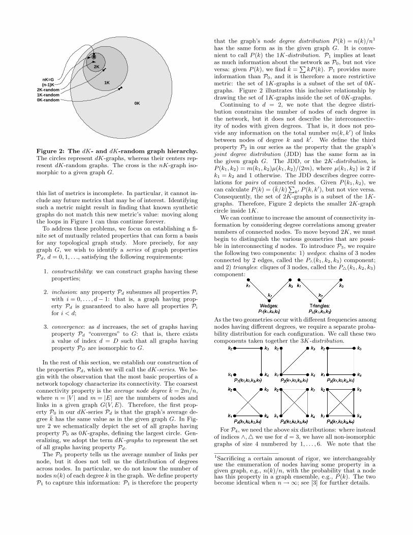
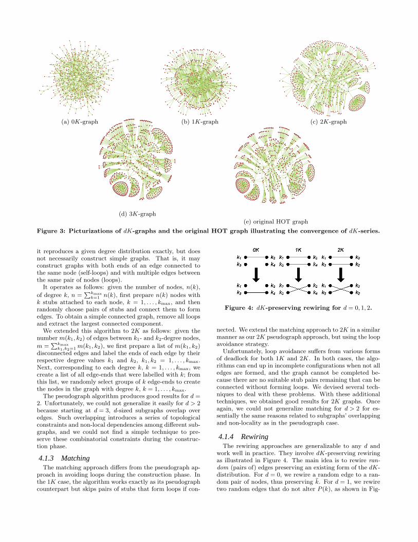
To motivate our ability to capture increasingly complexgraph properties by increasing d, we present visualizationsof dK-graphs generated using the dK-randomizing approachwe will discuss in Section 4.1.4. Figure 3 depicts random0K-, 1K-, 2K- and 3K-graphs matching the corresponding

distributions of the HOT graph, a representative router-leveltopology from [19]. This topology is particularly interesting,because, to date reproducing router-level topologies usingonly degree distributions has proven difficult [19]. However,a visual inspection of our generated topologies shows goodconvergence properties of the dK-series: while the 0K-graphand 1K-graph have little resemblance with the HOT topol-ogy, the 2K-graph is much closer than the previous ones andthe 3K graph is almost identical to the original. Althoughthe visual inspection is encouraging, we defer more carefulcomparisons to Section 5.

4. CONSTRUCTING dK-GRAPHSThere are several approaches for constructing dK-graphs

for d = 0 and d = 1. We extended a number of these algo-rithms to work for higher values of d. In Section 4.1, wedescribe these approaches, their practical utility, and ournew algorithms for d > 1. In Section 4.2, we introduce theconcept of dK-random graphs, in Section 4.3, a dK-space

exploration methodology. We use this methodology to de-termine the lowest values of d such that dK-graphs approxi-mate a given topology with the required degree of accuracy.

4.1 dK-graph-constructing algorithmsWe classify existing approaches to constructing 0K- and

1K-graphs into the following categories: stochastic, pseu-

dograph, matching, and two types of rewiring: randomizing

and targeting. We attempted to extend each of these tech-niques to general dK-graph construction. In this section, wequalitatively discuss the relative merits of each of these ap-proaches before presenting a more quantitative comparisonin Section 5.

4.1.1 StochasticThe simplest and most convenient for theoretical analysis

is the stochastic approach. For 0K, reproducing an n-sizedgraph with a given expected average degree k involves con-necting every pair of n nodes with probability p0K = k/n.This construction forms the classical (Erdos-Renyi) randomgraphs Gn,p [12]. Recent efforts have extended this stochas-tic approach to 1K and 2K [2, 7, 9]. In these cases, one firstlabels all nodes i with their expected degrees qi drawn fromthe distribution P (k) and then connects pairs of nodes (i, j)with probabilities p1K(qi, qj) = qiqj/(nq) or p2K(qi, qj) =(q/n)P (qi, qj)/(P (qi)P (qj)) reproducing the expected val-ues of 1K- or 2K-distributions, respectively.

In theory, we could generalize this approach for any din two stages: 1) extraction: given a graph G, calculatethe frequencies of all (including disconnected) d-sized sub-graphs in G, and 2) construction: prepare an n-sized set ofqi-labeled nodes and connect their d-sized subsets into dif-ferent subgraphs with (conditional) probabilities based onthe calculated frequencies. In practice, we find the stochas-tic approach performs poorly even for 1K because of highstatistical variance. For example, many nodes with expecteddegree 1 wind up with degree 0 after the construction phase,resulting in many tiny connected components.

4.1.2 PseudographThe pseudograph (also known as configuration) approach

is probably the most popular and widely used class of graph-generating algorithms. In its original form [1, 24], it appliesonly to the 1K case. Relative to the stochastic approach,

(a) 0K-graph (b) 1K-graph (c) 2K-graph

(d) 3K-graph

(e) original HOT graph

Figure 3: Picturizations of dK-graphs and the original HOT graph illustrating the convergence of dK-series.

it reproduces a given degree distribution exactly, but doesnot necessarily construct simple graphs. That is, it mayconstruct graphs with both ends of an edge connected tothe same node (self-loops) and with multiple edges betweenthe same pair of nodes (loops).

It operates as follows: given the number of nodes, n(k),

of degree k, n =Pkmax

k=1 n(k), first prepare n(k) nodes withk stubs attached to each node, k = 1, . . . , kmax, and thenrandomly choose pairs of stubs and connect them to formedges. To obtain a simple connected graph, remove all loopsand extract the largest connected component.

We extended this algorithm to 2K as follows: given thenumber m(k1, k2) of edges between k1- and k2-degree nodes,

m =Pkmax

k1,k2=1 m(k1, k2), we first prepare a list of m(k1, k2)disconnected edges and label the ends of each edge by theirrespective degree values k1 and k2, k1, k2 = 1, . . . , kmax.Next, corresponding to each degree k, k = 1, . . . , kmax, wecreate a list of all edge-ends that were labelled with k; fromthis list, we randomly select groups of k edge-ends to createthe nodes in the graph with degree k, k = 1, . . . , kmax.

The pseudograph algorithm produces good results for d =2. Unfortunately, we could not generalize it easily for d > 2because starting at d = 3, d-sized subgraphs overlap overedges. Such overlapping introduces a series of topologicalconstraints and non-local dependencies among different sub-graphs, and we could not find a simple technique to pre-serve these combinatorial constraints during the construc-tion phase.

4.1.3 MatchingThe matching approach differs from the pseudograph ap-

proach in avoiding loops during the construction phase. Inthe 1K case, the algorithm works exactly as its pseudographcounterpart but skips pairs of stubs that form loops if con-

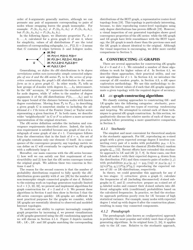
Figure 4: dK-preserving rewiring for d = 0, 1, 2.

nected. We extend the matching approach to 2K in a similarmanner as our 2K pseudograph approach, but using the loopavoidance strategy.

Unfortunately, loop avoidance suffers from various formsof deadlock for both 1K and 2K. In both cases, the algo-rithms can end up in incomplete configurations when not alledges are formed, and the graph cannot be completed be-cause there are no suitable stub pairs remaining that can beconnected without forming loops. We devised several tech-niques to deal with these problems. With these additionaltechniques, we obtained good results for 2K graphs. Onceagain, we could not generalize matching for d > 2 for es-sentially the same reasons related to subgraphs’ overlappingand non-locality as in the pseudograph case.

4.1.4 RewiringThe rewiring approaches are generalizable to any d and

work well in practice. They involve dK-preserving rewiringas illustrated in Figure 4. The main idea is to rewire ran-

dom (pairs of) edges preserving an existing form of the dK-distribution. For d = 0, we rewire a random edge to a ran-dom pair of nodes, thus preserving k. For d = 1, we rewiretwo random edges that do not alter P (k), as shown in Fig-

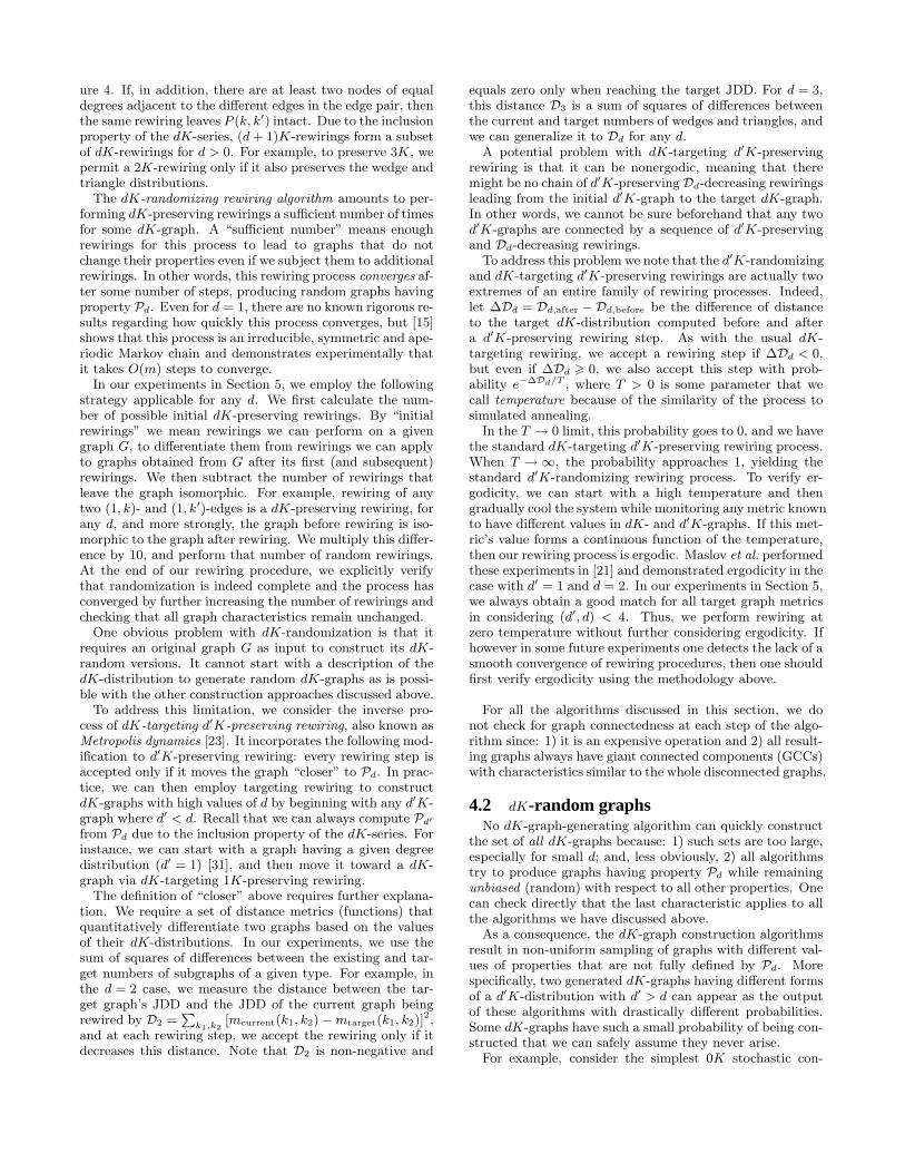
ure 4. If, in addition, there are at least two nodes of equaldegrees adjacent to the different edges in the edge pair, thenthe same rewiring leaves P (k, k′) intact. Due to the inclusionproperty of the dK-series, (d + 1)K-rewirings form a subsetof dK-rewirings for d > 0. For example, to preserve 3K, wepermit a 2K-rewiring only if it also preserves the wedge andtriangle distributions.

The dK-randomizing rewiring algorithm amounts to per-forming dK-preserving rewirings a sufficient number of timesfor some dK-graph. A “sufficient number” means enoughrewirings for this process to lead to graphs that do notchange their properties even if we subject them to additionalrewirings. In other words, this rewiring process converges af-ter some number of steps, producing random graphs havingproperty Pd. Even for d = 1, there are no known rigorous re-sults regarding how quickly this process converges, but [15]shows that this process is an irreducible, symmetric and ape-riodic Markov chain and demonstrates experimentally thatit takes O(m) steps to converge.

In our experiments in Section 5, we employ the followingstrategy applicable for any d. We first calculate the num-ber of possible initial dK-preserving rewirings. By “initialrewirings” we mean rewirings we can perform on a givengraph G, to differentiate them from rewirings we can applyto graphs obtained from G after its first (and subsequent)rewirings. We then subtract the number of rewirings thatleave the graph isomorphic. For example, rewiring of anytwo (1, k)- and (1, k′)-edges is a dK-preserving rewiring, forany d, and more strongly, the graph before rewiring is iso-morphic to the graph after rewiring. We multiply this differ-ence by 10, and perform that number of random rewirings.At the end of our rewiring procedure, we explicitly verifythat randomization is indeed complete and the process hasconverged by further increasing the number of rewirings andchecking that all graph characteristics remain unchanged.

One obvious problem with dK-randomization is that itrequires an original graph G as input to construct its dK-random versions. It cannot start with a description of thedK-distribution to generate random dK-graphs as is possi-ble with the other construction approaches discussed above.

To address this limitation, we consider the inverse pro-cess of dK-targeting d′K-preserving rewiring, also known asMetropolis dynamics [23]. It incorporates the following mod-ification to d′K-preserving rewiring: every rewiring step isaccepted only if it moves the graph “closer” to Pd. In prac-tice, we can then employ targeting rewiring to constructdK-graphs with high values of d by beginning with any d′K-graph where d′ < d. Recall that we can always compute Pd′

from Pd due to the inclusion property of the dK-series. Forinstance, we can start with a graph having a given degreedistribution (d′ = 1) [31], and then move it toward a dK-graph via dK-targeting 1K-preserving rewiring.

The definition of “closer” above requires further explana-tion. We require a set of distance metrics (functions) thatquantitatively differentiate two graphs based on the valuesof their dK-distributions. In our experiments, we use thesum of squares of differences between the existing and tar-get numbers of subgraphs of a given type. For example, inthe d = 2 case, we measure the distance between the tar-get graph’s JDD and the JDD of the current graph beingrewired by D2 =

P

k1,k2[mcurrent(k1, k2) − mtarget(k1, k2)]

2,and at each rewiring step, we accept the rewiring only if itdecreases this distance. Note that D2 is non-negative and

equals zero only when reaching the target JDD. For d = 3,this distance D3 is a sum of squares of differences betweenthe current and target numbers of wedges and triangles, andwe can generalize it to Dd for any d.

A potential problem with dK-targeting d′K-preservingrewiring is that it can be nonergodic, meaning that theremight be no chain of d′K-preserving Dd-decreasing rewiringsleading from the initial d′K-graph to the target dK-graph.In other words, we cannot be sure beforehand that any twod′K-graphs are connected by a sequence of d′K-preservingand Dd-decreasing rewirings.

To address this problem we note that the d′K-randomizingand dK-targeting d′K-preserving rewirings are actually twoextremes of an entire family of rewiring processes. Indeed,let ∆Dd = Dd,after −Dd,before be the difference of distanceto the target dK-distribution computed before and aftera d′K-preserving rewiring step. As with the usual dK-targeting rewiring, we accept a rewiring step if ∆Dd < 0,but even if ∆Dd > 0, we also accept this step with prob-ability e−∆Dd/T , where T > 0 is some parameter that wecall temperature because of the similarity of the process tosimulated annealing.

In the T → 0 limit, this probability goes to 0, and we havethe standard dK-targeting d′K-preserving rewiring process.When T → ∞, the probability approaches 1, yielding thestandard d′K-randomizing rewiring process. To verify er-godicity, we can start with a high temperature and thengradually cool the system while monitoring any metric knownto have different values in dK- and d′K-graphs. If this met-ric’s value forms a continuous function of the temperature,then our rewiring process is ergodic. Maslov et al. performedthese experiments in [21] and demonstrated ergodicity in thecase with d′ = 1 and d = 2. In our experiments in Section 5,we always obtain a good match for all target graph metricsin considering (d′, d) < 4. Thus, we perform rewiring atzero temperature without further considering ergodicity. Ifhowever in some future experiments one detects the lack of asmooth convergence of rewiring procedures, then one shouldfirst verify ergodicity using the methodology above.

For all the algorithms discussed in this section, we donot check for graph connectedness at each step of the algo-rithm since: 1) it is an expensive operation and 2) all result-ing graphs always have giant connected components (GCCs)with characteristics similar to the whole disconnected graphs.

4.2 dK-random graphsNo dK-graph-generating algorithm can quickly construct

the set of all dK-graphs because: 1) such sets are too large,especially for small d; and, less obviously, 2) all algorithmstry to produce graphs having property Pd while remainingunbiased (random) with respect to all other properties. Onecan check directly that the last characteristic applies to allthe algorithms we have discussed above.

As a consequence, the dK-graph construction algorithmsresult in non-uniform sampling of graphs with different val-ues of properties that are not fully defined by Pd. Morespecifically, two generated dK-graphs having different formsof a d′K-distribution with d′ > d can appear as the outputof these algorithms with drastically different probabilities.Some dK-graphs have such a small probability of being con-structed that we can safely assume they never arise.

For example, consider the simplest 0K stochastic con-

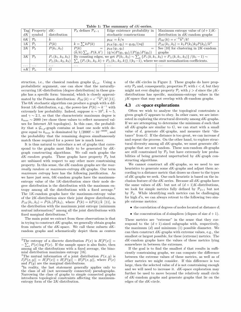
Table 1: The summary of dK-series.

TagdK

Propertysymbol

dK-distribution

Pd defines Pd−1 Edge existence probability instochastic constructions

Maximum entropy value of (d+1)K-distribution in dK-random graphs

0K P0 k p0K = k/n P0K(k) = e−kkk/k!1K P1 P (k) k =

P

kP (k) p1K(q1, q2) = q1q2/(nq) P1K(k1, k2) = k1P (k1)k2P (k2)/k2

2K P2 P (k1, k2) P (k) =(k/k)

P

k′ P (k, k′)p2K(q1, q2) =(q/n)P (q1, q2)/(P (q1)P (q2))

See [10] for clustering in 2K-randomgraphs

3K P3 P∧(k1, k2, k3)P△(k1, k2, k3)

By counting edges, we get P (k1, k2) ∼P

k {P∧(k, k1, k2) + P△(k, k1, k2)} /(k1 − 1) ∼P

k {P∧(k1, k2, k) + P△(k1, k2, k)} /(k2−1), where we omit normalization coefficients.. . . . . . . . . . . . . . . . . .nK Pn G

struction, i.e., the classical random graphs Gn,p. Using aprobabilistic argument, one can show that the naturally-occurring 1K-distribution (degree distribution) in these gra-phs has a specific form: binomial, which is closely approxi-

mated by the Poisson distribution: P0K(k) = e−kkk/k! [11].The 0K stochastic algorithm can produce a graph with a dif-ferent 1K-distribution, e.g., the power-law P (k) ∼ k−γ withextremely low probability. Indeed, suppose n ∼ 104, k ∼ 5,and γ ∼ 2.1, so that the characteristic maximum degree iskmax ∼ 2000 (we chose these values to reflect measured val-ues for Internet AS topologies). In this case, the probabil-ity that a Gn,p-graph contains at least one node with de-gree equal to kmax is dominated by 1/2000! ∼ 10−6600, andthe probability that the remaining degrees simultaneouslymatch those required for a power law is much lower.

It is thus natural to introduce a set of graphs that corre-spond to the graphs most likely to be generated by dK-graph constructing algorithms. We call such graphs thedK-random graphs. These graphs have property Pd butare unbiased with respect to any other more constrainingproperty. In this sense, the dK-random graphs are the max-

imally random or maximum-entropy dK-graphs. Our termmaximum entropy here has the following justification. Aswe have just seen, 0K-random graphs have the maximum-entropy value of the 1K-distribution since their node de-gree distribution is the distribution with the maximum en-tropy among all the distributions with a fixed average.2

The 1K-random graphs have the maximum-entropy valueof the 2K-distribution since their joint degree distribution,P1K(k1, k2) = P (k1)P (k2), where P (k) = kP (k)/k [11], isthe distribution with the maximum joint entropy (minimummutual information)3 among all the joint distributions withfixed marginal distributions.4

The main point we extract from these observations is thatin trying to construct dK-graphs, we generally obtain graphsfrom subsets of the dK-space. We call these subsets dK-random graphs and schematically depict them as centers

2The entropy of a discrete distribution P (x) is H[P (x)] =−

P

x P (x) log P (x). If the sample space is also finite, thenamong all the distributions with a fixed average, the bino-mial distribution maximizes entropy [16].3The mutual information of a joint distribution P (x, y) isI[P (x, y)] = H[P (x)] + H[P (y)] − H[P (x, y)], where P (x)and P (y) are the marginal distributions.4In reality, the last statement generally applies only tothe class of all (not necessarily connected) pseudographs.Narrowing the class of graphs to simple connected graphsintroduces topological constraints affecting the maximum-entropy form of the 2K-distribution.

of the dK-circles in Figure 2. These graphs do have prop-erty Pd and, consequently, properties Pi with i < d, but theymight not ever display property Pj with j > d since the jK-distributions has specific, maximum-entropy values in thejK-space that may not overlap with dk-random graphs.

4.3 dK-space explorationsOften we wish to analyze the topological constraints a

given graph G appears to obey. In other cases, we are inter-ested in exploring the structural diversity among dK-graphs.If we are attempting to determine the minimum d such thatall dK-graphs are similar to G, we can start with a smallvalue of d, generate dK-graphs, and measure their “dis-tance” from G. If the distance is too great, we can increase dand repeat the process. On the other hand, to explore struc-tural diversity among all dK-graphs, we must generate dK-graphs that are not random. These non-random dk-graphsare still constrained by Pd but have extremely low proba-bilities of being generated unperturbed by dK-graph con-structing algorithms.

We cannot construct all dK-graphs, so we need to useheuristics to generate some dK-graphs and adjust them ac-cording to a distance metric that draws us closer to the typesof dK-graphs we seek. One such heuristic is based on the in-clusion feature of the dK-series. Because all dK-graphs havethe same values of dK- but not of (d + 1)K-distributions,we look for simple metrics fully defined by Pd+1 but notby Pd. While identifying such metrics can be challengingfor high d’s, we can always retreat to the following two sim-ple extreme metrics:

• the correlation of degrees of nodes located at distance d;

• the concentration of d-simplices (cliques of size d + 1).

These metrics are “extreme” in the sense that they cor-respond to the (d + 1)-sized subgraphs with, respectively,the maximum (d) and minimum (1) possible diameter. Wecan then construct dK-graphs with extreme values, e.g., thesmallest or largest possible, for these (extreme) metrics. ThedK-random graphs have the values of these metrics lyingsomewhere in between the extremes.

If the goal is to find the smallest d that results in suffi-ciently constraining graphs, we can compute the differencebetween the extreme values of these metrics, as well as ofother metrics we might consider. If this difference is toolarge, then the selected value of d is not constraining enoughand we will need to increase it. dK-space exploration mayfurther be used to move beyond the relatively small circleof dK-random graphs and generate graphs that lie on theedges of the dK-circle.

To illustrate this approach in practice, we consider 1K-and 2K-space explorations. For 1K, the simplest metricdefined by P2 is any scalar summary statistics of the 2K-distribution, such as likelihood S (cf. Section 2). To con-struct graphs with the maximum value of S, we can run aform of targeting 1K-preserving rewiring that accepts eachrewiring step only if it increases S. We can perform the op-posite to minimize S. This type of experiment was at thecore of recent work that led the authors of [19] to concludethat d = 1 was not constraining enough for the topologythey considered.

To perform 2K-space explorations, we need to find simplescalar metrics defined by P3. Since the 3K-distribution isactually two distributions, P∧(k1, k2, k3) and P△(k1, k2, k3),we should have two independent scalar metrics. The second-

order likelihood S2 is one such metric for P∧(k1, k2, k3).S2 ∼

P

k1,k2,k3k1k3P∧(k1, k2, k3); we define S2 as the sum

of the products of degrees of nodes located at the ends ofwedges, so that any two graphs with the same P∧(k1, k2, k3)have the same S2. For the P△(k1, k2, k3) component, av-erage clustering C ∼

P

k1,k2,k3k1P△(k1, k2, k3) is an ap-

propriate candidate. We note that these two metrics arealso the two extreme metrics in the sense defined above:S2 measures the properly normalized correlation of degreesof nodes located at distance 2, while C describes the con-centration of 2-simplices (triangles). The 2K-explorationsamount then to performing the following two types of tar-geting 2K-preserving rewiring: accept a 2K-rewiring steponly if it maximizes or minimizes: 1) S2, or 2) C.

5. EVALUATIONIn this section, we conduct a number of experiments to

demonstrate the ability of the dK-series to capture impor-tant graph properties. We implemented all the dK-graph-constructing algorithms from Section 4.1, applied them toboth measured and modeled Internet topologies, and calcu-lated all the topology metrics from Section 2 on the resultinggraphs.

We experimented with three measured AS-level topolo-gies, extracted from CAIDA’s skitter traceroute [5], Route-Views’ BGP [26], and RIPE’s WHOIS [17] data for themonth of March 2004, as well as with a synthetic router-level topology—the HOT graph from [19]. The qualitativeresults of our experiments are similar for the skitter andBGP topologies, while the WHOIS topology lies somewherein-between the skitter/BGP and HOT topologies. In thecase of skitter comprising of 9204 nodes and 28959 edges,we will see that its degree distribution places significant con-straints upon the graph generation process. Thus, even 1K-random graphs approximate the skitter topology reasonablywell. The HOT topology with 939 nodes and 988 edges isat the opposite extreme. It is the least constrained; 1K-random graphs approximate it poorly, and dK-series’ con-vergence is slowest. We thus report results only for thesetwo extreme cases, skitter and HOT.

Our results represent averages over 100 graphs generatedwith a different random seed in each case, using the notationin Table 2.

5.1 Algorithmic ComparisonWe first compare the different graph generation algorithms

discussed in Section 4.1. All the algorithms give consistentresults, except the stochastic approach, which suffers from

Table 2: Scalar graph metrics notations.

Metric NotationAverage degree kAssortativity coefficient rAverage clustering CAverage distance dStandard deviation of distance distribution σd

Second-order likelihood S2

Smallest eigenvalue of the Laplacian λ1

Largest eigenvalue of the Laplacian λn−1

Table 3: Scalar metrics for 2K-random HOT graphs

generated using different techniques.

Met- Stoch- Pseu- Match- 2K- 2K- Orig.ric astic dogr. ing rand. targ. HOTk 2.87 2.19 2.22 2.18 2.18 2.10r -0.22 -0.24 -0.21 -0.23 -0.24 -0.22d 4.99 6.25 6.22 6.32 6.35 6.81σd 0.85 0.75 0.74 0.70 0.70 0.57

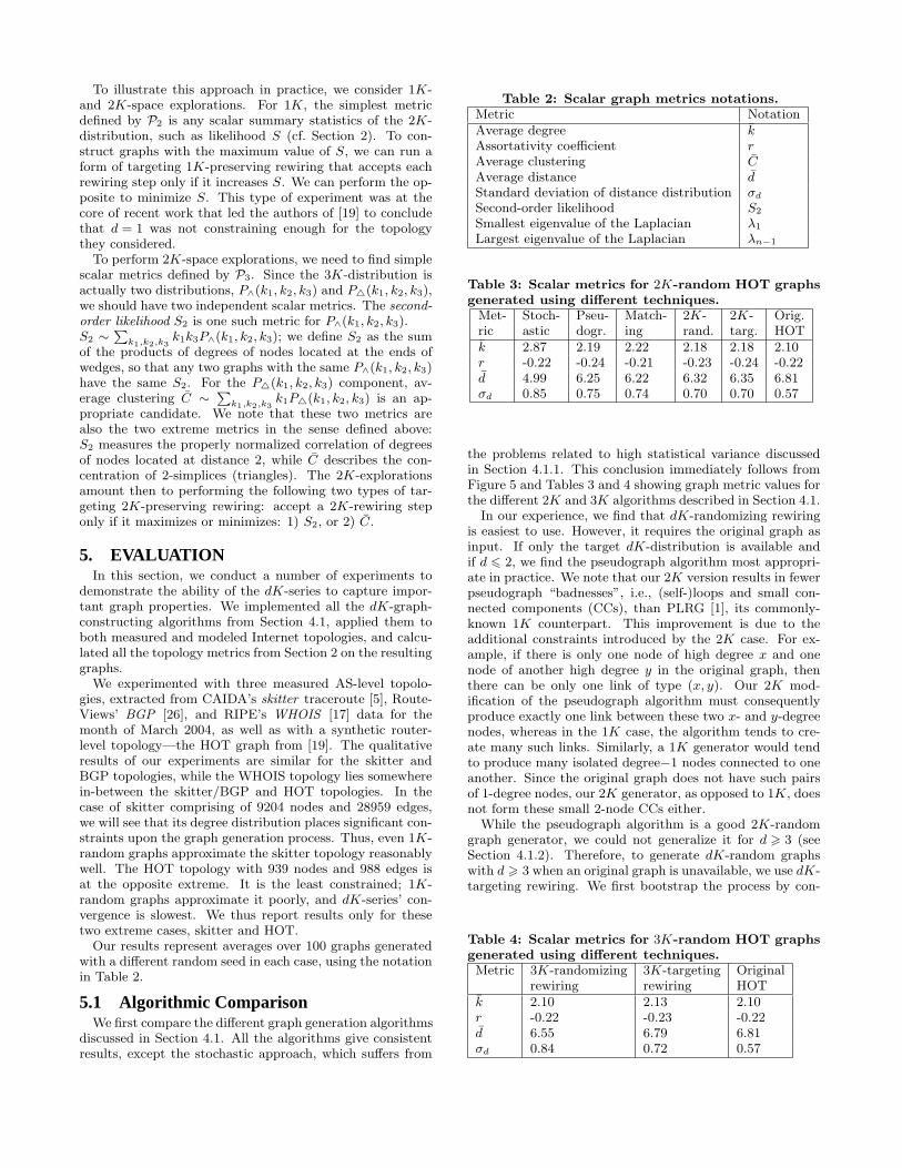
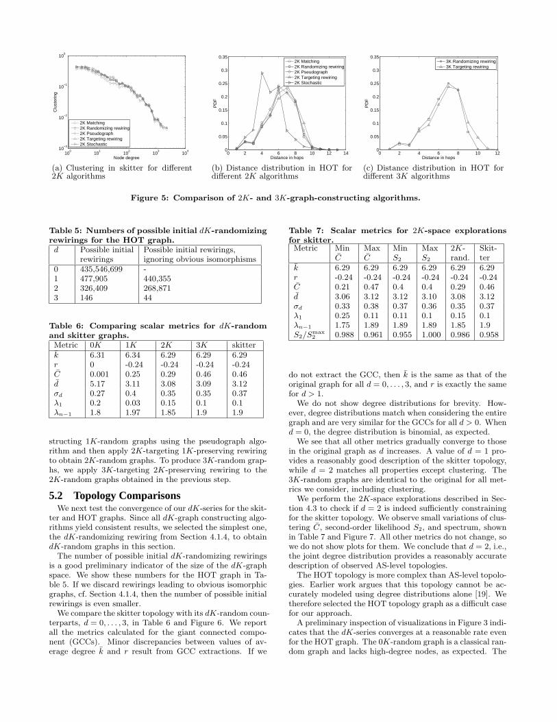
the problems related to high statistical variance discussedin Section 4.1.1. This conclusion immediately follows fromFigure 5 and Tables 3 and 4 showing graph metric values forthe different 2K and 3K algorithms described in Section 4.1.

In our experience, we find that dK-randomizing rewiringis easiest to use. However, it requires the original graph asinput. If only the target dK-distribution is available andif d 6 2, we find the pseudograph algorithm most appropri-ate in practice. We note that our 2K version results in fewerpseudograph “badnesses”, i.e., (self-)loops and small con-nected components (CCs), than PLRG [1], its commonly-known 1K counterpart. This improvement is due to theadditional constraints introduced by the 2K case. For ex-ample, if there is only one node of high degree x and onenode of another high degree y in the original graph, thenthere can be only one link of type (x, y). Our 2K mod-ification of the pseudograph algorithm must consequentlyproduce exactly one link between these two x- and y-degreenodes, whereas in the 1K case, the algorithm tends to cre-ate many such links. Similarly, a 1K generator would tendto produce many isolated degree−1 nodes connected to oneanother. Since the original graph does not have such pairsof 1-degree nodes, our 2K generator, as opposed to 1K, doesnot form these small 2-node CCs either.

While the pseudograph algorithm is a good 2K-randomgraph generator, we could not generalize it for d > 3 (seeSection 4.1.2). Therefore, to generate dK-random graphswith d > 3 when an original graph is unavailable, we use dK-targeting rewiring. We first bootstrap the process by con-

Table 4: Scalar metrics for 3K-random HOT graphs

generated using different techniques.

Metric 3K-randomizing 3K-targeting Originalrewiring rewiring HOT

k 2.10 2.13 2.10r -0.22 -0.23 -0.22d 6.55 6.79 6.81σd 0.84 0.72 0.57

100

101

102

103

104

10−3

10−2

10−1

100

Node degree

Clu

ster

ing

2K Matching2K Randomizing rewiring2K Pseudograph2K Targeting rewiring2K Stochastic

(a) Clustering in skitter for different2K algorithms

0 2 4 6 8 10 12 140

0.05

0.1

0.15

0.2

0.25

0.3

0.35

Distance in hops

PD

F

2K Matching2K Randomizing rewiring2K Pseudograph2K Targeting rewiring2K Stochastic

(b) Distance distribution in HOT fordifferent 2K algorithms

0 2 4 6 8 10 120

0.05

0.1

0.15

0.2

0.25

0.3

0.35

Distance in hops

PD

F

3K Randomizing rewiring3K Targeting rewiring

(c) Distance distribution in HOT fordifferent 3K algorithms

Figure 5: Comparison of 2K- and 3K-graph-constructing algorithms.

Table 5: Numbers of possible initial dK-randomizing

rewirings for the HOT graph.

d Possible initial Possible initial rewirings,rewirings ignoring obvious isomorphisms

0 435,546,699 -1 477,905 440,3552 326,409 268,8713 146 44

Table 6: Comparing scalar metrics for dK-random

and skitter graphs.

Metric 0K 1K 2K 3K skitterk 6.31 6.34 6.29 6.29 6.29r 0 -0.24 -0.24 -0.24 -0.24C 0.001 0.25 0.29 0.46 0.46d 5.17 3.11 3.08 3.09 3.12σd 0.27 0.4 0.35 0.35 0.37λ1 0.2 0.03 0.15 0.1 0.1λn−1 1.8 1.97 1.85 1.9 1.9

structing 1K-random graphs using the pseudograph algo-rithm and then apply 2K-targeting 1K-preserving rewiringto obtain 2K-random graphs. To produce 3K-random grap-hs, we apply 3K-targeting 2K-preserving rewiring to the2K-random graphs obtained in the previous step.

5.2 Topology ComparisonsWe next test the convergence of our dK-series for the skit-

ter and HOT graphs. Since all dK-graph constructing algo-rithms yield consistent results, we selected the simplest one,the dK-randomizing rewiring from Section 4.1.4, to obtaindK-random graphs in this section.

The number of possible initial dK-randomizing rewiringsis a good preliminary indicator of the size of the dK-graphspace. We show these numbers for the HOT graph in Ta-ble 5. If we discard rewirings leading to obvious isomorphicgraphs, cf. Section 4.1.4, then the number of possible initialrewirings is even smaller.

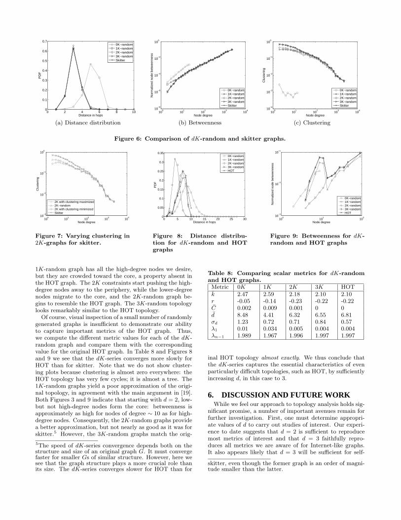
We compare the skitter topology with its dK-random coun-terparts, d = 0, . . . , 3, in Table 6 and Figure 6. We reportall the metrics calculated for the giant connected compo-nent (GCCs). Minor discrepancies between values of av-erage degree k and r result from GCC extractions. If we

Table 7: Scalar metrics for 2K-space explorations

for skitter.Metric Min Max Min Max 2K- Skit-

C C S2 S2 rand. terk 6.29 6.29 6.29 6.29 6.29 6.29r -0.24 -0.24 -0.24 -0.24 -0.24 -0.24C 0.21 0.47 0.4 0.4 0.29 0.46d 3.06 3.12 3.12 3.10 3.08 3.12σd 0.33 0.38 0.37 0.36 0.35 0.37λ1 0.25 0.11 0.11 0.1 0.15 0.1λn−1 1.75 1.89 1.89 1.89 1.85 1.9S2/Smax

2 0.988 0.961 0.955 1.000 0.986 0.958

do not extract the GCC, then k is the same as that of theoriginal graph for all d = 0, . . . , 3, and r is exactly the samefor d > 1.

We do not show degree distributions for brevity. How-ever, degree distributions match when considering the entiregraph and are very similar for the GCCs for all d > 0. Whend = 0, the degree distribution is binomial, as expected.

We see that all other metrics gradually converge to thosein the original graph as d increases. A value of d = 1 pro-vides a reasonably good description of the skitter topology,while d = 2 matches all properties except clustering. The3K-random graphs are identical to the original for all met-rics we consider, including clustering.

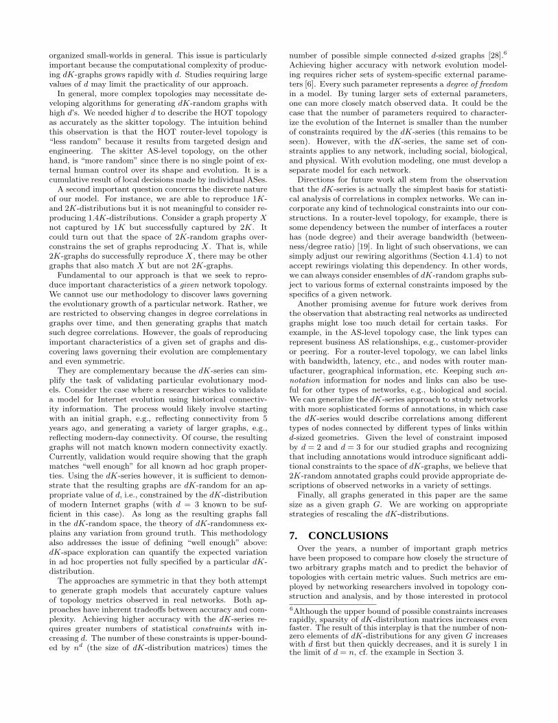
We perform the 2K-space explorations described in Sec-tion 4.3 to check if d = 2 is indeed sufficiently constrainingfor the skitter topology. We observe small variations of clus-tering C, second-order likelihood S2, and spectrum, shownin Table 7 and Figure 7. All other metrics do not change, sowe do not show plots for them. We conclude that d = 2, i.e.,the joint degree distribution provides a reasonably accuratedescription of observed AS-level topologies.

The HOT topology is more complex than AS-level topolo-gies. Earlier work argues that this topology cannot be ac-curately modeled using degree distributions alone [19]. Wetherefore selected the HOT topology graph as a difficult casefor our approach.

A preliminary inspection of visualizations in Figure 3 indi-cates that the dK-series converges at a reasonable rate evenfor the HOT graph. The 0K-random graph is a classical ran-dom graph and lacks high-degree nodes, as expected. The

0 2 4 6 8 100

0.1

0.2

0.3

0.4

0.5

0.6

0.7

Distance in hops

PD

F

0K−random1K−random2K−random3K−randomSkitter

(a) Distance distribution

100

101

102

103

104

10−8

10−6

10−4

10−2

100

Node degree

Nor

mal

ized

nod

e be

twee

nnes

s

0K−random1K−random2K−random3K−randomSkitter

(b) Betweenness

100

101

102

103

104

10−4

10−3

10−2

10−1

100

Node degree

Clu

ster

ing

0K−random1K−random2K−random3K−randomSkitter

(c) Clustering

Figure 6: Comparison of dK-random and skitter graphs.

100

101

102

103

104

10−3

10−2

10−1

100

Node degree

Clu

ster

ing

2K with clustering maximized2K−random2K with clustering minimizedSkitter

Figure 7: Varying clustering in

2K-graphs for skitter.

0 5 10 15 20 25 300

0.05

0.1

0.15

0.2

0.25

0.3

0.35

Distance in hops

PD

F

0K−random1K−random2K−random3K−randomHOT

Figure 8: Distance distribu-

tion for dK-random and HOT

graphs

100

101

102

10−3

10−2

10−1

Node degree

Nor

mal

ized

nod

e be

twee

nnes

s

0K−random1K−random2K−random3K−randomHOT

Figure 9: Betweenness for dK-

random and HOT graphs

1K-random graph has all the high-degree nodes we desire,but they are crowded toward the core, a property absent inthe HOT graph. The 2K constraints start pushing the high-degree nodes away to the periphery, while the lower-degreenodes migrate to the core, and the 2K-random graph be-gins to resemble the HOT graph. The 3K-random topologylooks remarkably similar to the HOT topology.

Of course, visual inspection of a small number of randomlygenerated graphs is insufficient to demonstrate our abilityto capture important metrics of the HOT graph. Thus,we compute the different metric values for each of the dK-random graph and compare them with the correspondingvalue for the original HOT graph. In Table 8 and Figures 8and 9 we see that the dK-series converges more slowly forHOT than for skitter. Note that we do not show cluster-ing plots because clustering is almost zero everywhere: theHOT topology has very few cycles; it is almost a tree. The1K-random graphs yield a poor approximation of the origi-nal topology, in agreement with the main argument in [19].Both Figures 3 and 9 indicate that starting with d = 2, low-but not high-degree nodes form the core: betweenness isapproximately as high for nodes of degree ∼ 10 as for high-degree nodes. Consequently, the 2K-random graphs providea better approximation, but not nearly as good as it was forskitter.5 However, the 3K-random graphs match the orig-

5The speed of dK-series convergence depends both on thestructure and size of an original graph G. It must convergefaster for smaller Gs of similar structure. However, here wesee that the graph structure plays a more crucial role thanits size. The dK-series converges slower for HOT than for

Table 8: Comparing scalar metrics for dK-random

and HOT graphs.

Metric 0K 1K 2K 3K HOTk 2.47 2.59 2.18 2.10 2.10r -0.05 -0.14 -0.23 -0.22 -0.22C 0.002 0.009 0.001 0 0d 8.48 4.41 6.32 6.55 6.81σd 1.23 0.72 0.71 0.84 0.57λ1 0.01 0.034 0.005 0.004 0.004λn−1 1.989 1.967 1.996 1.997 1.997

inal HOT topology almost exactly. We thus conclude thatthe dK-series captures the essential characteristics of evenparticularly difficult topologies, such as HOT, by sufficientlyincreasing d, in this case to 3.

6. DISCUSSION AND FUTURE WORKWhile we feel our approach to topology analysis holds sig-

nificant promise, a number of important avenues remain forfurther investigation. First, one must determine appropri-ate values of d to carry out studies of interest. Our experi-ence to date suggests that d = 2 is sufficient to reproducemost metrics of interest and that d = 3 faithfully repro-duces all metrics we are aware of for Internet-like graphs.It also appears likely that d = 3 will be sufficient for self-

skitter, even though the former graph is an order of magni-tude smaller than the latter.

organized small-worlds in general. This issue is particularlyimportant because the computational complexity of produc-ing dK-graphs grows rapidly with d. Studies requiring largevalues of d may limit the practicality of our approach.

In general, more complex topologies may necessitate de-veloping algorithms for generating dK-random graphs withhigh d’s. We needed higher d to describe the HOT topologyas accurately as the skitter topology. The intuition behindthis observation is that the HOT router-level topology is“less random” because it results from targeted design andengineering. The skitter AS-level topology, on the otherhand, is “more random” since there is no single point of ex-ternal human control over its shape and evolution. It is acumulative result of local decisions made by individual ASes.

A second important question concerns the discrete natureof our model. For instance, we are able to reproduce 1K-and 2K-distributions but it is not meaningful to consider re-producing 1.4K-distributions. Consider a graph property Xnot captured by 1K but successfully captured by 2K. Itcould turn out that the space of 2K-random graphs over-constrains the set of graphs reproducing X. That is, while2K-graphs do successfully reproduce X, there may be othergraphs that also match X but are not 2K-graphs.

Fundamental to our approach is that we seek to repro-duce important characteristics of a given network topology.We cannot use our methodology to discover laws governingthe evolutionary growth of a particular network. Rather, weare restricted to observing changes in degree correlations ingraphs over time, and then generating graphs that matchsuch degree correlations. However, the goals of reproducingimportant characteristics of a given set of graphs and dis-covering laws governing their evolution are complementaryand even symmetric.

They are complementary because the dK-series can sim-plify the task of validating particular evolutionary mod-els. Consider the case where a researcher wishes to validatea model for Internet evolution using historical connectiv-ity information. The process would likely involve startingwith an initial graph, e.g., reflecting connectivity from 5years ago, and generating a variety of larger graphs, e.g.,reflecting modern-day connectivity. Of course, the resultinggraphs will not match known modern connectivity exactly.Currently, validation would require showing that the graphmatches “well enough” for all known ad hoc graph proper-ties. Using the dK-series however, it is sufficient to demon-strate that the resulting graphs are dK-random for an ap-propriate value of d, i.e., constrained by the dK-distributionof modern Internet graphs (with d = 3 known to be suf-ficient in this case). As long as the resulting graphs fallin the dK-random space, the theory of dK-randomness ex-plains any variation from ground truth. This methodologyalso addresses the issue of defining “well enough” above:dK-space exploration can quantify the expected variationin ad hoc properties not fully specified by a particular dK-distribution.

The approaches are symmetric in that they both attemptto generate graph models that accurately capture valuesof topology metrics observed in real networks. Both ap-proaches have inherent tradeoffs between accuracy and com-plexity. Achieving higher accuracy with the dK-series re-quires greater numbers of statistical constraints with in-creasing d. The number of these constraints is upper-bound-ed by nd (the size of dK-distribution matrices) times the

number of possible simple connected d-sized graphs [28].6

Achieving higher accuracy with network evolution model-ing requires richer sets of system-specific external parame-ters [6]. Every such parameter represents a degree of freedom

in a model. By tuning larger sets of external parameters,one can more closely match observed data. It could be thecase that the number of parameters required to character-ize the evolution of the Internet is smaller than the numberof constraints required by the dK-series (this remains to beseen). However, with the dK-series, the same set of con-straints applies to any network, including social, biological,and physical. With evolution modeling, one must develop aseparate model for each network.

Directions for future work all stem from the observationthat the dK-series is actually the simplest basis for statisti-cal analysis of correlations in complex networks. We can in-corporate any kind of technological constraints into our con-structions. In a router-level topology, for example, there issome dependency between the number of interfaces a routerhas (node degree) and their average bandwidth (between-ness/degree ratio) [19]. In light of such observations, we cansimply adjust our rewiring algorithms (Section 4.1.4) to notaccept rewirings violating this dependency. In other words,we can always consider ensembles of dK-random graphs sub-ject to various forms of external constraints imposed by thespecifics of a given network.

Another promising avenue for future work derives fromthe observation that abstracting real networks as undirectedgraphs might lose too much detail for certain tasks. Forexample, in the AS-level topology case, the link types canrepresent business AS relationships, e.g., customer-provideror peering. For a router-level topology, we can label linkswith bandwidth, latency, etc., and nodes with router man-ufacturer, geographical information, etc. Keeping such an-

notation information for nodes and links can also be use-ful for other types of networks, e.g., biological and social.We can generalize the dK-series approach to study networkswith more sophisticated forms of annotations, in which casethe dK-series would describe correlations among differenttypes of nodes connected by different types of links withind-sized geometries. Given the level of constraint imposedby d = 2 and d = 3 for our studied graphs and recognizingthat including annotations would introduce significant addi-tional constraints to the space of dK-graphs, we believe that2K-random annotated graphs could provide appropriate de-scriptions of observed networks in a variety of settings.

Finally, all graphs generated in this paper are the samesize as a given graph G. We are working on appropriatestrategies of rescaling the dK-distributions.

7. CONCLUSIONSOver the years, a number of important graph metrics

have been proposed to compare how closely the structure oftwo arbitrary graphs match and to predict the behavior oftopologies with certain metric values. Such metrics are em-ployed by networking researchers involved in topology con-struction and analysis, and by those interested in protocol

6Although the upper bound of possible constraints increasesrapidly, sparsity of dK-distribution matrices increases evenfaster. The result of this interplay is that the number of non-zero elements of dK-distributions for any given G increaseswith d first but then quickly decreases, and it is surely 1 inthe limit of d = n, cf. the example in Section 3.

and distributed system performance. Unfortunately, thereis limited understanding of which metrics are appropriatefor a given setting and, for most proposed metrics, there areno known algorithms for generating graphs that reproducethe target property.

This paper defines a series of graph structural propertiesto both systematically characterize arbitrary graphs and togenerate random graphs that match specified characteristicsof the original. The dK-distribution is a collection of distri-butions describing the correlations of degrees of d connectednodes. The properties Pd, d = 0, . . . , n, comprise the dK-series. A random graph is said to have property Pd if itsdK-distribution has the same form as in a given graph G.By increasing the value of d in the series, it is possible tocapture more complex properties of G and, in the limit,a sufficiently large value of d yields complete informationabout G’s structure.

We find interesting tradeoffs in choosing the appropri-ate value of d to compare two graphs or to generate ran-dom graphs with property Pd. As we increase d, the set ofrandomly generated graphs having property Pd becomes in-creasingly constrained and the resulting graphs are increas-ingly likely to reproduce a variety of metrics of interest. Atthe same time, the algorithmic complexity associated withgenerating the graphs increases sharply. Thus, we present amethodology where practitioners choose the smallest d thatcaptures essential graph characteristics for their study. Forthe graphs that we consider, including comparatively com-plex Internet AS- and router-level topologies, we find thatd = 2 is sufficient for most cases and d = 3 captures allgraph properties proposed in the literature known to us.

In this paper, we present the first algorithms for construct-ing random graphs having properties P2 and P3, and sketchan approach for extending the algorithms to arbitrary d. Weare also releasing the source code for our analysis tools tomeasure an input graph’s dK-distribution and our genera-tor able to produce random graphs possessing properties Pd

for d < 4.We hope that our methodology will provide a more rig-

orous and consistent method of comparing topology graphsand enable protocol and application researchers to test sys-tem behavior under a suite of randomly generated yet ap-propriately constrained and realistic network topologies.

AcknowledgementsWe would like to thank Walter Willinger and Lun Li fortheir HOT topology data; Bradley Huffaker, David Moore,Marina Fomenkov, and kc claffy for their contributions atdifferent stages of this work; and anonymous reviewers fortheir comments that helped to improve the final version ofthis manuscript. Support for this work was provided by NSFCNS-0434996 and Center for Networked Systems (CNS) atUCSD.

8. REFERENCES[1] W. Aiello, F. Chung, and L. Lu. A random graph model for

massive graphs. In STOC, 2000.

[2] M. Boguna and R. Pastor-Satorras. Class of correlated randomnetworks with hidden variables. Physical Review E, 68:036112,2003.

[3] M. Boguna, R. Pastor-Satorras, and A. Vespignani. Cut-offsand finite size effects in scale-free networks. European PhysicalJournal B, 38:205–209, 2004.

[4] T. Bu and D. Towsley. On distinguishing between Internetpower law topology generators. In INFOCOM, 2002.

[5] CAIDA. Macroscopic topology AS adjacencies. http://www.caida.org/tools/measurement/skitter/as adjacencies.xml.

[6] H. Chang, S. Jamin, and W. Willinger. To peer or not to peer:Modeling the evolution of the Internet’s AS-level topology. InINFOCOM, 2006.

[7] F. Chung and L. Lu. Connected components in random graphswith given degree sequences. Annals of Combinatorics,6:125–145, 2002.

[8] F. K. R. Chung. Spectral Graph Theory, volume 92 of RegionalConference Series in Mathematics. American MathematicalSociety, Providence, RI, 1997.

[9] S. N. Dorogovtsev. Networks with given correlations.http://arxiv.org/abs/cond-mat/0308336v1.

[10] S. N. Dorogovtsev. Clustering of correlated networks. PhysicalReview E, 69:027104, 2004.

[11] S. N. Dorogovtsev and J. F. F. Mendes. Evolution ofNetworks: From Biological Nets to the Internet and WWW.Oxford University Press, Oxford, 2003.

[12] P. Erdos and A. Renyi. On random graphs. PublicationesMathematicae, 6:290–297, 1959.

[13] M. Faloutsos, P. Faloutsos, and C. Faloutsos. On power-lawrelationships of the Internet topology. In SIGCOMM, 1999.

[14] P. Fraigniaud. A new perspective on the small-worldphenomenon: Greedy routing in tree-decomposed graphs. InESA, 2005.

[15] C. Gkantsidis, M. Mihail, and E. Zegura. The Markovsimulation method for generating connected power law randomgraphs. In ALENEX, 2003.

[16] P. Harremoes. Binomial and Poisson distributions as maximumentropy distributions. Transactions on Information Theory,47(5):2039–2041, 2001.

[17] Internet Routing Registries. http://www.irr.net/.

[18] D. Krioukov, K. Fall, and X. Yang. Compact routing onInternet-like graphs. In INFOCOM, 2004.

[19] L. Li, D. Alderson, W. Willinger, and J. Doyle. Afirst-principles approach to understanding the Internetsrouter-level topology. In SIGCOMM, 2004.

[20] P. Mahadevan, D. Krioukov, M. Fomenkov, B. Huffaker,X. Dimitropoulos, kc claffy, and A. Vahdat. The InternetAS-level topology: Three data sources and one definitivemetric. Computer Communication Review, 36(1), 2006.

[21] S. Maslov, K. Sneppen, and A. Zaliznyak. Detection oftopological patterns in complex networks: Correlation profile ofthe Internet. Physica A, 333:529–540, 2004.

[22] A. Medina, A. Lakhina, I. Matta, and J. Byers. BRITE: Anapproach to universal topology generation. In MASCOTS,2001.

[23] N. Metropolis, A. Rosenbluth, M. Rosenbluth, A. Teller, andE. Teller. Equation-of-state calculations by fast computingmachines. Journal of Chemical Physics, 21:1087, 1953.

[24] M. Molloy and B. Reed. A critical point for random graphswith a given degree sequence. Random Structures andAlgorithms, 6:161–179, 1995.

[25] M. E. J. Newman. Assortative mixing in networks. PhysicalReview Letters, 89:208701, 2002.

[26] University of Oregon RouteViews Project.http://www.routeviews.org/.

[27] M. A. Serrano and M. Boguna. Tuning clustering in randomnetworks with arbitrary degree distributions. Physical ReviewE, 72:036133, 2005.

[28] N. J. A. Sloane. Sequence A001349. The On-Line Encyclopediaof Integer Sequences.http://www.research.att.com/projects/OEIS?Anum=A001349.

[29] H. Tangmunarunkit, R. Govindan, S. Jamin, S. Shenker, andW. Willinger. Network topology generators: Degree-based vs.structural. In SIGCOMM, 2002.

[30] A. Vazquez, R. Pastor-Satorras, and A. Vespignani. Large-scaletopological and dynamical properties of the Internet. PhysicalReview E, 65:066130, 2002.

[31] F. Viger and M. Latapy. Efficient and simple generation ofrandom simple connected graphs with prescribed degreesequence. In COCOON, 2005.

[32] J. Winick and S. Jamin. Inet-3.0: Internet topology generator.Technical Report UM-CSE-TR-456-02, University of Michigan,2002.