Systematic Uncertainties Associated withthe Cosmological Analysis of the First

Pan-STARRS1 Type Ia Supernova SampleThe Harvard community has made this

article openly available. Please share howthis access benefits you. Your story matters

Citation Scolnic, D., A. Rest, A. Riess, M. E. Huber, R. J. Foley, D. Brout,R. Chornock, et al. 2014. Systematic Uncertainties Associatedwith the Cosmological Analysis of the First Pan-STARRS1 TypeIa Supernova Sample. The Astrophysical Journal 795, no. 1: 45.doi:10.1088/0004-637x/795/1/45.

Published Version doi:10.1088/0004-637x/795/1/45

Citable link http://nrs.harvard.edu/urn-3:HUL.InstRepos:30496614

Terms of Use This article was downloaded from Harvard University’s DASHrepository, and is made available under the terms and conditionsapplicable to Open Access Policy Articles, as set forth at http://nrs.harvard.edu/urn-3:HUL.InstRepos:dash.current.terms-of-use#OAP

September 3, 2014Preprint typeset using LATEX style emulateapj v. 5/2/11

SYSTEMATIC UNCERTAINTIES ASSOCIATED WITH THE COSMOLOGICAL ANALYSIS OF THE FIRSTPAN-STARRS1 TYPE IA SUPERNOVA SAMPLE

D. Scolnic1, A. Rest2, A. Riess1, M. E. Huber3, R. J. Foley4,5,6, D. Brout1, R. Chornock4, G. Narayan7, J. L.Tonry3, E. Berger4, A. M. Soderberg4, C. W. Stubbs7,4, R. P. Kirshner4,7, S. Rodney1, S. J. Smartt8, E.

Schlafly9, M. T. Botticella8, P. Challis4, I. Czekala4, M. Drout4, M.J. Hudson10, R. Kotak8, C. Leibler11, R.Lunnan4, G. H. Marion4, M. McCrum8, D. Milisavljevic4, A. Pastorello13, N. E. Sanders4, K. Smith8, E.

Stafford1, D. Thilker1, S. Valenti14,15, W. M. Wood-Vasey16, Z. Zheng1, W. S. Burgett3, K. C. Chambers3, L.Denneau3, P. W. Draper17, H. Flewelling3, K. W. Hodapp3, N. Kaiser3, R.-P. Kudritzki3, E. A. Magnier3, N.

Metcalfe17, P. A. Price12, W. Sweeney3, R. Wainscoat3, C. Waters3.

September 3, 2014

ABSTRACT

We probe the systematic uncertainties from the 113 Type Ia supernovae (SN Ia) in thePan-STARRS1 (PS1) sample along with 197 SN Ia from a combination of low-redshift surveys. Thecompanion paper by Rest et al. (2013) describes the photometric measurements and cosmologicalinferences from the PS1 sample. The largest systematic uncertainty stems from the photometric cal-ibration of the PS1 and low-z samples. We increase the sample of observed Calspec standards from7 to 10 used to define the PS1 calibration system. The PS1 and SDSS-II calibration systems arecompared and discrepancies up to ∼ 0.02 mag are recovered. We find uncertainties in the proper wayto treat intrinsic colors and reddening produce differences in the recovered value of w up to 3%. Weestimate masses of host galaxies of PS1 supernovae and detect an insignificant difference in distanceresiduals of the full sample of 0.037±0.031 mag for host galaxies with high and low masses. Assumingflatness and including systematic uncertainties in our analysis of only SNe measurements, we findw =−1.120+0.360

−0.206(Stat)+0.269−0.291(Sys). With additional constraints from BAO, CMB (Planck) and H0

measurements, we find w = −1.166+0.072−0.069 and Ωm = 0.280+0.013

−0.012 (statistical and systematic errorsadded in quadrature). Significance of the inconsistency with w = −1 depends on whether we usePlanck or WMAP measurements of the CMB: wBAO+H0+SN+WMAP = −1.124+0.083

−0.065.

Subject headings: supernova general–cosmology observations–cosmological parameters

1. INTRODUCTION

1 Department of Physics and Astronomy, Johns Hopkins Uni-versity, 3400 North Charles Street, Baltimore, MD 21218, USA

2 Space Telescope Science Institute, 3700 San Martin Drive,Baltimore, MD 21218, USA

3 Institute for Astronomy, University of Hawaii, 2680 Wood-lawn Drive, Honolulu, HI 96822, USA

4 Harvard-Smithsonian Center for Astrophysics, 60 GardenStreet, Cambridge, MA 02138, USA

5 Astronomy Department, University of Illinois at Urbana-Champaign, 1002 West Green Street, Urbana, IL 61801, USA

6 Department of Physics, University of Illinois Urbana-Champaign, 1110 W. Green Street, Urbana, IL 61801, USA

7 Department of Physics, Harvard University, 17 OxfordStreet, Cambridge MA 02138

8 Astrophysics Research Centre, School of Mathematics andPhysics, Queens University Belfast, Belfast, BT71NN, UK

9 Max Planck Institute for Astronomy, K onigstuhl 17, D-69117 Heidelberg, Germany

10 University of Waterloo, 200 University Ave W Waterloo,ON N2L 3G1, Canada

11 Department of Astronomy & Astrophysics, University ofCalifornia, Santa Cruz, CA 95060, USA

12 Department of Astrophysical Sciences, Princeton Univer-sity, Princeton, NJ 08544, USA

13 INAF - Osservatorio Astronomico di Padova, Vicolodell’Osservatorio 5, 35122 Padova, Italy

14 Las Cumbres Observatory Global Telescope Network, Inc.,Santa Barbara, CA 93117, USA

15 Department of Physics, University of California Santa Bar-bara, Santa Barbara, CA 93106-9530, USA

16 PITT PACC, Department of Physics and Astronomy, Uni-versity of Pittsburgh, Pittsburgh, PA 15260, USA.

17 Department of Physics, University of Durham Science Lab-oratories, South Road Durham DH1 3LE, UK

One of the main goals of the Pan-STARRS1 (PS1)Medium Deep survey is to detect and monitor thousandsof SN Ia in order to measure the equation of state param-eter of dark energy, w = P/ρc2 (where P is pressure andρ is density). The first results of this effort are reportedin the companion paper by Rest et al. (2013, hereafterR14). For PS1 and other new surveys to advance our un-derstanding of dark energy, the flood of new SNe mustbe accompanied by similar improvement in the reductionof systematic uncertainties.

Since the initial discovery of cosmic acceleration (Riesset al. 1998, Perlmutter et al. 1999), there have been manysupernova surveys utilizing multiple passbands and densetime-sampling at both low-z (e.g., CSP,CfA1-4, LOSS,SNFactory18) and at intermediate and higher-z (e.g.,SDSS, ESSENCE, SNLS19). While the sample sizes haveincreased, the systematic uncertainties of these samplesnow are of nearly equal value to the statistical uncertain-ties (Conley et al. 2011; hereafter C11). Nearly all of thesystematic uncertainties in the analysis of these samplesfall into a small handful of categories: calibration, selec-tion effects, correlated flows, extinction corrections andlight curve modeling. There has been significant recent

18 Carnegie Supernova Project (CSP), Center for Astrophysics(CfA), Lick Observatory Supernova Search (LOSS), Nearby Super-nova Factory (NSF)

19 Sloan Digital Sky Survey (SDSS),Equation of State: SupEr-Novae trace Cosmic Expansion (ESSENCE), SuperNova LegacySurvey (SNLS)

arX

iv:1

310.

3824

v2 [

astr

o-ph

.CO

] 2

Sep

201

4

2 Scolnic, Rest et al

progress in understanding each of them. For example,recent studies suggest that properties of host galaxiesof SNe appear to be correlated with distance residualsrelative to a best fit cosmology (e.g., Kelly et al. 2010,Sullivan et al. 2010a, Lampeitl et al. 2010). Other stud-ies have shown that supernova colors and brightnesses,long thought to be inconsistent with a Milky Way (MW)-like reddening law, can be explained by a MW-like dustmodel (Folatelli et al. 2010, Foley & Kasen 2011, Mandel,Narayan & Kirshner 2011, Chotard et al. 2011, Scolnicet al. 2013).

The PS1 Medium Deep Survey has discovered over1700 SN candidates in its first 1.5 years. Of these,146 SNe were spectroscopically identified as Type Ia.Well-sampled multi-band light curves with near-peak ob-servations were measured for 113 of the spectroscopicallyconfirmed sample. We include a low-z sample of 197 SNeto improve our cosmological constraints. The companionpaper by R14 analyzes the photometry of the PS1 lightcurves, presents the light curve fit parameters and de-rives constraints on w from a combined data set of PS1SNe and low-z SNe (hereafter PS1+lz). In this paper,we augment the work of R14 with a more comprehen-sive analysis of the systematic uncertainties of w. Val-ues of the matter density Ωm and equation-of-state ware recovered with constraints from SNe alone and whenwe include constraints from measurements of the CosmicMicrowave Background (CMB), Baryon Acoustic Oscil-lation (BAO) and the Hubble Constant.

In section §2, we present an overview of the major sys-tematic uncertainties in our sample, and detail the twoapproaches towards quantifying these uncertainties. Insection §3 we analyze the photometric calibration of PS1and attempt to reconcile the reported calibration dis-crepancies (Tonry et al. 2012, hereafter T12) betweenPS1 and SDSS. We also discuss the data sets in PS1+lzand tension between the various samples. Accurate sim-ulations of the PS1 survey and expected selection effectsfor each of the surveys in the combined PS1+lz are givenin §4. In §5 we probe the validity of the two major as-sumptions of the SALT2 light curve fitter for determin-ing distances to SNe. In §6 we analyze coherent flows ofthe combined sample for the PS1+lz sample. Changesto Milky Way extinction maps are presented in §7. Ourreview and discussion of the dominant uncertainties isgiven in §8 and our conclusions are in §9.

2. OVERALL SYSTEMATICS REVIEW

2.1. Data

The sample analyzed in this paper includes SN Ia dis-covered by PS1 and observed in low-z follow-up pro-grams. We apply the same selection criteria for the qual-ity and coverage of the light curve observations to thesesamples as was done in R14. As detailed in R14, thelow-z SN sample is selected from six different samples:Calan/Tololo [16 SNe] (Hamuy et al. 1996), CfA1 [5 SNe](Riess et al. 1999), CfA2 [19 SNe] (Jha et al. 2006), CfA3[85 SNe] (Hicken et al. 2009a), CSP [45] (Contreras et al.2010) and CfA4 [43 SNe] (Hicken et al. 2009b). We alsoinclude supernovae not discovered in these surveys butcollected as part of the JRK07 (Jha, Riess, & Kirshner2007) paper [8 SNe]. The PS1 sample contains 113 SNeafter selection cuts. While the focus of this paper will be

on the PS1+low-z sample, we will compare results withthe SDSS (Holtzman et al. 2008) and SNLS (Guy et al.2010) samples. For these samples, we apply the sameselection criteria from R14. We make all data used inthis analysis publicly available, including light curve fitparameters20.

External constraints from CMB, BAO and H0 mea-surements are described in detail in R14. For all thesemeasurements, we use the Markov chains derived byPlanck Collaboration et al. (2013). The Planck data setthat is quoted includes data from the Planck temperaturepower spectrum data, Planck temperature data, Plancklensing, and WMAP polarization at low multipoles. TheBAO measurement quoted is from the aggregate of BAOmeasurements of different surveys, as compiled by PlanckCollaboration et al. (2013) and listed in R14. The H0

measurement is from Riess et al. (2011).

2.2. Potential Sources of Systematic Errors

Here, we briefly enumerate the dominant systematicuncertainties in the PS1+lz sample.

Calibration. Flux calibration errors are typically thelargest source of systematic uncertainty in any super-nova sample (C11). The original PS1 photometric sys-tem (T12) is based on accurate filter measurements ob-tained in situ. T12 adjusts the throughput of these mea-surements on a < 3% scale for better agreement betweensynthetic and photometric observations of Hubble SpaceTelescope (HST) Calspec standards Bohlin (1996)21. Inthis paper, we increase the size of the sample of Calspecstandards that underpin the HST flux scale from 7 to 10(adding five, but eliminating two) to reduce the uncer-tainty in the calibration.

We call the improved photometric system usedthroughout this paper the PS1 14 calibration system.For the low-z samples, we follow the C11 treatment ofphotometric systems. For our total calibration uncer-tainty, we combine uncertainties from the HST Calspecand Landolt standards, as well as the uncertainties inmeasurements of the bandpasses and zeropoints. We alsoexplore noted discrepancies between the PS1 and SDSSphotometric systems.

Selection Effects. Selection effects can bias amagnitude-limited survey, due either to detection lim-its or selection of the objects for spectroscopic follow-up.The SNANA simulator22 (Kessler et al. 2009b) allows usto use actual observing conditions, cadence, and spectro-scopic efficiency to mimic our survey. The spectroscopicefficiency of a survey is particularly difficult to formalizeif the survey does not have a single consistent follow-upprogram that is based on well-defined criteria for select-ing targets.

We correct for PS1 selection effects by incorporatingthe observing history into a simulation and identifyingthe effective selection criteria that best match the data.For the low-z sample, we follow the same approach. Forour systematic uncertainty, we explore how well our sim-ulations match the data.

Light-curve Fitting. To optimize the use of SN Ia asstandard candles to determine distances, most light curve

20 http://ps1sc.org/transients/21 http://www.stsci.edu/hst/observatory/cdbs/calspec.html22 SNANA v10 23 @ http://www.sdss.org/supernova/SNANA.html

Systematic Uncertainties of PS1 Sample 3

fitters correct the observed peak magnitude of the SNusing the width and color of the light curve. Whileeach fitter accounts in some way for a light curve shape-luminosity relation (Phillips 1993) to correct for thewidth of the light curve, there is a disagreement betweenfitters about the best manner to correct for the color ofthe light curve. Using SNANA’s fitter with the SALT2model (Guy et al. 2010) as the primary light curve fitter,recently Scolnic et al. (hereafter, S13) showed that thereis a degeneracy between models of SN color when the in-trinsic scatter of SN Ia is mostly composed of luminosityvariation or color variation.

The primary method for determining distances usesSALT2 to find light curve parameters and afterwardscorrects the distances with the average bias from sim-ulations based on these two models of SN color. For oursystematic uncertainty, we explore the difference in dis-tances between the two models from when we take theaverage.

Host Galaxy Relations. Multiple studies have shownrelations between various host galaxy properties andHubble residuals (e.g., Kelly et al. 2010, Sullivan et al.2010a, Lampeitl et al. 2010). However, there is noconsensus about which host galaxy property is directlylinked to luminosity (Childress et al. 2013), or whetherthese correlations may be artifacts of light curve correc-tions (Kim et al. 2013).

The primary fit does not include any corrections toSN Ia distances for host galaxy properties. For our sys-tematic uncertainty, we explore whether correcting thedistances of the SNe in the PS1+lz sample by includinginformation about host galaxies properties is statisticallysignificant.

MW Extinction Corrections. For each SN, we cor-rect for the MW extinction at its specific sky location.Our primary fit uses values from Schlegel, Finkbeiner,& Davis (1998), with corrections from Schlafly &Finkbeiner (2011) and the restriction that E(B − V ) <0.5 in the direction of the SN. We include systematic un-certainties in the extinction correction from uncertaintiesin the subtraction of the zodiacal light, temperature cor-rections, and the non-linearity of extinction corrections(Schlafly & Finkbeiner 2011).

Coherent Velocity Flows. To account for density fluc-tuations, we correct the redshift of each SN for coher-ent flows (Hudson et al. 2004). The primary fit correctsall redshifts for coherent flows starting at zmin = 0.01.For our systematic uncertainty, we measure the changein recovered cosmological parameters when we vary theminimum redshift of the sample.

Other Uncertainties not analyzed in this paper, butconsidered in other studies, include contamination byother types of SN, SN evolution, and gravitational lens-ing. Contamination by other types of SN was alreadydiscussed in R14, and we apply the same treatmenthere. While gravitational lensing should increase theamount of dispersion of the SN Ia distances at high-zσµlens = 0.055z (Jonsson et al. 2010), selection effectsdominate any trend seen at high-z in the PS1 sample.For SN evolution, this uncertainty is already included inthe light curve modeling uncertainty.

Finally, while we include cosmological constraints fromthe Planck survey (Planck Collaboration et al. 2013), toaddress systematics in external data sets we compare the

results when we include constraints from WMAP (Hin-shaw et al. 2012).

2.3. Error Propagation

To determine the entire systematic uncertainty of wfrom the PS1+lz sample, we follow two different ap-proaches towards error accounting. The first approachfollows C11, determining a covariance matrix that in-cludes uncertainties from multiple sources. The secondapproach is similar to that of Riess et al. (2011), whichfinds the variations of cosmological constraints due tovariants in the analysis. For example, in the secondmethod one may find the different values of w usingthe PS1 calibration system as stated, or when modi-fied to match the SDSS photometric system. In the firstmethod, the errors from the PS1 calibration system arepropagated. Since there are a number of discrete choicesof how to do steps of the analysis in this paper, we incor-porate both methods of error accounting. Each of thesemethods is different from the conventional method thatadds all the systematic errors in quadrature at the endof the analysis.

The advantage of the approach shown in C11 is that itproperly accounts for covariances between SNe and alsofor interactions between systematic uncertainties. Thefull covariance error matrix is given as:

C = Dstat + Csys. (1)

where Dstat is a diagonal matrix with each element con-sisting of the square of the intrinsic dispersion of the sam-ple σ2

int and the square of the noise error σ2n for each SN.

Csys is the systematic covariance matrix. C11 furtherseparates Csys into two components, only one of whichmay be further reduced with more SNe. For simplicity,we do not separate these components. Given the Trippestimator (Tripp 1998) and using SALT2 to fit the lightcurve,

µ = mB + α× x1 − β × c−M, (2)

where mB is the peak brightness of the SN, x1 is thestretch of the light curve, c is the color of the light curve,and α, β and M are nuisance parameters. Explanationof the derivations of α and β is given in R14. The sys-tematic covariance, for a vector of distances ~µ, betweenthe i’th and j’th SN is calculated as:

Cij,sys =

K∑k=1

(∂µi∂Sk

)(∂µj∂Sk

)(σSk

)2, (3)

where the sum is over the K systematics Sk, σSkis the

magnitude of each systematic error, and ∂µ is defined asthe difference in distance modulus values after changingone of the systematic parameters. For example, in orderto determine the covariance matrix due to a systematicerror of 0.01 mag in the transmission function of rp1 fil-ter, we refit all of the SNe light curves after adding 0.01mag to the zeropoint of all observed rp1 values. Follow-ing C11, we do not fix α and β when we propagate thesystematic covariance matrix. α and β are derived withSALT2mu (Marriner et al. 2011) in the statistical case,though when including the covariance matrix, we write acompatible routine that allows off-diagonal elements. Asgiven in R14 (Table 4), when attributing the remainingintrinsic scatter to luminosity variation (σint = 0.115),

4 Scolnic, Rest et al

α and β are found to be 0.147 ± 0.010 and 3.13 ± 0.12respectively.

Given a vector of distance residuals for the SN sample∆~µ = ~µ−~µ(H0,ΩM ,ΩΛ, w, ~z) then χ2 may be expressedas

χ2 = ∆~µT ·C−1 ·∆~µ. (4)

We minimize Eqn. 4 to determine cosmological param-eters that include H0,ΩM ,ΩΛ and w. The cosmologicalparameters are defined in R14 - Eq. 3. All cosmologi-cal parameters quoted in this pair of papers are of themarginalized values and not the minimum χ2 values. Weassess the impact of each systematic uncertainty by ex-amining the shift it produces in the inferred cosmologicalparameters. We also compute the “relative area” whichwe define as the area of the contour that encloses 68.3%of the probability distribution between w and ΩM com-pared to when only including statistical uncertainties.For this analysis, we assume that the universe is flat. Itis worth clarifying that the relative area may decrease asthe contours shift in w vs. ΩM space, so relative areaalone does not quantify the entire effect of a systematicerror.

In the second approach, we redetermine distancesbased on variations (often binary) in the analysis meth-ods (e.g. Riess et al. 2011). Unlike the method by C11,there is no systematic error component to the error ma-trix in Eqn. 3. Instead, cosmological parameters arefound for each difference in analysis approaches. Theoverall systematic uncertainty of w from this method isthe standard deviation of values for w from the variantsto the primary fit.

3. SYSTEMATIC UNCERTAINTIES IN THE ABSOLUTECALIBRATION

The flux calibration of PS1 measurements relies onan iterative process that includes work from T12 andSchlafly et al. (2012) and is built on by this work andthat of R14. T12 observes several HST Calspec stan-dards (Bohlin 1996) with PS1 and compares the observedmagnitudes of these standards to the predicted magni-tudes from synthetic photometry. T12 finds the AB off-sets so that the observed magnitudes best matches thesynthetic photometry, given tight constraints from mea-surements on the bandpass edges and shapes. Catalogsfrom the fields that contain the Calspec standards arethen included as a basis of the relative calibration per-formed by Schlafly et al. (2012), which uses repeat PS1observations of stars and solves simultaneously for thesystem throughput, the atmospheric transparency, andthe large-scale detector flat field (called ‘ubercal’). Inthis process, new sky catalogs are created not only forthe fields in which the Calspec standards are located, butacross the entire observable sky including the MediumDeep fields.

The original observations of Calspec standards by T12are supplemented by observations of those and other Cal-spec standards as part of the Pan-STARRs 3Pi survey.In this work, we determine the AB offsets between theobserved magnitudes of the entire set of Calspec stan-dards calibrated by ubercal and the synthetic photom-etry of these standards. This iterative process is thusa more accurate test of the absolute flux calibration ofPS1. Once these offsets are found, R14 applies the off-sets to the Medium Deep field catalogs, and analyzes

further calibration uncertainties that may affect the SNmeasurements. Zeropoints for the nightly photometry ofthe supernovae are determined by comparing the pho-tometry of a single image to the photometry from theMedium Deep field catalog at that location.

The main demarcation between the analysis of Rest etal. and Scolnic et al. when analyzing the calibration un-certainties is that Rest et al. analyzes the uncertaintiesin the photometric measurements of the stars and super-novae, while Scolnic et al. focus on how these uncertain-ties propagate to measurements of the absolute calibra-tion of the PS1 system and the supernova distances.

3.1. Overview of Calibration Uncertainties

Uncertainties in the calibration of the various samplescomprise the largest systematic uncertainty in our analy-sis. In Fig. 1, we show a schematic describing the calibra-tion of the various subsamples. The overall systematicuncertainty in the calibration of our combined PS1+lzsample may be expressed as the combination of threeuncertainties. The first component encompasses system-atic uncertainties in the nightly photometry and how wellthe filter bandpasses are measured. For the PS1 sam-ple, R14 presents analysis of the systematic uncertaintydue to spatial and temporal uncertainties in the nightlyphotometry. T12 presents the uncertainty in how wellthe bandpasses are measured (uncertainty of filter edges< 7 A). T12 also analyzes uncertainty in the atmosphericattenuation compensation for the filter zeropoints.

Spatial and temporal variation of the filter bandpassespropagate into our total calibration uncertainty in threeways: how the catalog photometry is determined, howthe photometry of the Calspec standards is determined,and how the photometry of the supernovae is determined.We expect that the uncertainty in the nightly zeropointsto be small. We find by comparing Pan-STARRs andSDSS photometry that any variation of the PS1 photom-etry across the focal plane for colors 0.4 < g − i < 1.5is less than 3mmag and is difficult to detect because ofnoise. The effect of variation of the filter bandpasses onphotometry of the Calspec standards and the supernovaeare significantly larger because of the very blue colors ofa large fraction of the Calspec standards and the narrowspectral features of these supernovae. These effects areboth considered.

The second major component of the total calibrationuncertainty is in determining the flux zeropoints of eachfilter based on observations of astronomical standards.Since the accuracy of the internal PS1 measurementsof the flux zeropoints is not better than 1%, the zero-points are adjusted so that the observed photometry ofHST Calspec standards (e.g., AB - HST Calspec; Bohlin1996) matches the synthetic photometry of these stan-dards. Analogously, for the low-z sample, this uncer-tainty encompasses the accuracy of the color transfor-mation of Landolt standards. For PS1, the adjustmentof the photometry to agree with the synthetic photome-try dominates the uncertainty in the filter measurementsby T12. Both uncertainties are included in our analysis.

The third main component of the total calibration un-certainty is the accuracy in the measurements of the stan-dard stars (e.g., HST Calspec or Landolt). This is com-posed of errors in the color of the standard stars and

Systematic Uncertainties of PS1 Sample 5

the absolute flux of the standards. For the PS1 sampleand select measurements in the low-z samples, this un-certainty is due to possible errors in measurements of theHST Calspec standards. For most of the low-z sample,this uncertainty is due to color and absolute flux errorsfrom the realization of the Vega23 magnitude system asimplemented in the standard catalogs of Landolt. A com-mon flux scale for the PS1 supernovae and low-z SNe canbe achieved by the binding between the Landolt catalogand Calspec standards (Landolt & Uomoto 2007). In afuture analysis, we plan to cross-calibrate the Landoltcatalog to the PS1 catalog to further improve the fluxscales of the different samples. If we limited our analy-sis to SNe from a single survey, the overall absolute fluxcalibration would be degenerate with the absolute peakmagnitude of SNe. But combining distance moduli ofSNe from multiple surveys requires that there is a com-mon absolute flux scale.

R14 presents an error budget for the PS1 photomet-ric system. Here we explain many of these uncertainties,along with uncertainties of the low-z calibration. We alsodetail the derivation of new zeropoint offsets for the PS1calibration that are used in R14. The total uncertaintyin the recovery of cosmological parameters due to cali-bration for the PS1+lz sample is given in Table 1. Foreach uncertainty described, this uncertainty is indepen-dently added to each observed magnitude of the SN, andthe light curves are refit. Afterwards, cosmological con-straints are redetermined.

3.2. Pan-STARRS Absolute Calibration

The Pan-STARRS AB magnitude system, as describedin T12, is based on small (< 0.03 mag) adjustmentsto highly accurate measurements of the PS1 systemthroughput and filter transmissions measured in situ.Perturbations to each filter transmission are optimized sothat ‘synthetic’ photometry, using measurements of filtertransmission throughputs and stellar spectra, agrees withobservations of HST Calspec standard stars. To do this,T12 analyzed the PS1 observations of 7 Calspec stan-dards, all observed on the same photometric night. Theerror in how well the Calspec SEDs are defined on the ABsystem as well as the offsets between the observed andsynthetic Calspec magnitudes represent the two largesterrors in the PS1 calibration system. T12 finds that theentire systematic uncertainty from absolute calibrationin each filter is ∼ 0.017 mag. We recalculate that valuehere.

Once the PS1 calibration is defined to be on the ABsystem, there is an uncertainty from the relative calibra-tion between the fields with Calspec standards to the restof the sky. To do the relative calibration, Schlafly et al.(2012) use repeat PS1 observations of stars. Star cata-logs created by this process are used in our supernovapipeline. Internal consistency tests show Schlafly et al.(2012) achieve field-to-field relative precision of < 0.01mag in gp1,rp1, and ip1 and ∼ 0.01 mag in zp1 . Theseerrors are included in our overall zeropoint uncertain-ties, after dividing by

√10 - the number of fields. While

a following discussion will focus on agreement betweenthe absolute calibration of PS1 and SDSS, it is worth

23 The absolute flux of Landolt standards is discussed at the endof the section.

PS1 CSP

CFA3-4S,

JRK07

-Filters griz ugri,BV BVRIri,BV

CFA4,

CFA3-Kep

Matc

hin

g I

nte

rnal

to

Ab

solu

te C

ali

bra

tion

Obs. 12 Calspec

Found AB offsets

Ubercal

Color transformations of Landolt

observations

-Method Laser/diode Laser/diodeLaser

/diode

-Nat. Syst. Yes Yes Yes Yes | No

Monochromatic

illumination diode

Ab

solu

te C

ali

bra

tion

-Absolute

Flux

StandardWD

standards

(C)

-WD

standards (C),

--

-Color of

Calibration

System Calspec

Color

Calspec Color,

BD17 (L)

BD17 (S),

BD17 (L)BD17 (L)

Obs. 1 Calspec

Found AB offsets (BD17), ..

Inte

rnal

Cali

bra

tion

Abs. Flux

Color

Standard

bandpass|

-

Fig. 1.— A schematic of the calibration of the PS1+lz sample.The calibration of the various subsamples is broken into three parts:‘Internal calibration’ (filter measurements), ‘match between Inter-nal and Absolute calibration’, and ‘Absolute calibration’. Arrowsshow whether in each step there may be an uncertainty due to acolor measurement or absolute flux measurement. Directionalityof absolute flux arrows show the source of the uncertainty. ‘C’, ‘L’and ‘S’ represent the HST Calspec, Landolt and Smith standardsrespectively.

mentioning that Schlafly et al. (2012) find greater inter-nal inconsistencies at the ∼ 0.01 mag level in the SDSSphotometry than in the PS1 photometry.

To improve the PS1 absolute calibration, we analyzea larger sample of Calspec standards that have been ob-served throughout the PS1 survey. In total, there are12 Calpsec standards that have been observed by PS1 ingrizp1 that are not saturated in the observations. Thesestandards were observed so that they avoided the directcenter of the focal plane, where there are some unre-solved discrepancies as described by R14. We measurethe PS1 magnitudes of the observed Calspec standardsin the same way as T12. We then apply a zeropoint offsetobtained by computing the difference of the magnitudesof stars in the fields with the stars in the full-sky star cat-alogs set by Schlafly et al. (2012). To avoid a Malmquistbias in the determination of the zeropoint, we empiricallydetermine the magnitude limit at which stars can be usedfor this comparison. We also remove any observations ofCalspec standards where there is greater than a 0.03 magdifference between the aperture and PSF photometry, aswe found this adequately removes any saturated observa-tions. As the Calspec standards observed are so bright,we follow T12 and include a 0.005 mag uncertainty toaccount for how some of the standards may be near thesaturation limit.

6 Scolnic, Rest et al

-1 0 1 2g-i (mag)

-0.015

-0.010

-0.005

0.000

0.005

0.010

0.015 g

-gc

en

t (m

ag

)

OuterMid

Center

StarCalspecSN

-1 0 1 2g-i (mag)

-0.015

-0.010

-0.005

0.000

0.005

0.010

0.015

r-r

ce

nt (m

ag

)

-1 0 1 2g-i (mag)

-0.015

-0.010

-0.005

0.000

0.005

0.010

0.015

i-i

ce

nt (m

ag

)

-1 0 1 2g-i (mag)

-0.015

-0.010

-0.005

0.000

0.005

0.010

0.015

z-z

ce

nt (m

ag

)

0.0 0.1 0.2 0.3 0.4 0.5 0.6 0.7z

-0.04

-0.02

0.00

0.02

0.04

∆ µ

Fig. 2.— (Top panels) The synthetic magnitude differences ofPickles stars, Calspec standards, and a SNIa at different redshiftswhen the object is observed near the center of the focal plane com-pared to in an outer annulus. The smooth change in color of theSNIa is due to red shifting a normal SNIa spectrum. Filter func-tions used in this process are from Tonry et al. 2011. (Bottompanel) Changes in distance found for PS1 SNe when the correctfilter function at the focal position is used versus the nominal po-sition.

To make full use of the observations of Calspec stan-dards, we must consider how the filter functions changeacross the focal plane. In Fig. 2, we show the changein synthetic magnitudes of stars in the Pickles’ library(Pickles 1998), Calspec standards and supernovae for agiven color and position on the focal plane. We findthe variation in synthetic magnitudes for supernovae andCalspec standards may be significantly larger than thevariation of stars in the narrow color range used to de-fine the stellar zeropoints. Therefore, given the measure-ments of filter functions across the focal plane (measuredat ∆r = 0.15 deg), we transform the observed magni-tudes of the Calspec standards to a uniform system de-fined at the center of the focal plane. As shown in Fig. . 2, this correction for the blue Calspec standards may beas large as 5 mmag. This approach is similar to that ofBetoule et al. (2012).

For each observation of a Calspec standard, we fol-low Schlafly et al. and assign an observational error of0.015 + σmag−psf , which Schlafly et al. finds adequatelydescribes the scatter seen in their star catalogs. To de-termine the net adjustment needed for each passband,we find the weighted difference of the observed and syn-thetic magnitudes of the Calspec standards. For thisprocess, we add an additional uncertainty of 0.008 magto each difference in order to represent the uncertainty inthe ubercal process. In Appendix A, we present the en-tire set of Calspec standards observed and their syntheticmagnitudes in the PS1 system24, as well as the observedmagnitudes. From Figure 3, we find that corrections

24 PS1 passbands can be found on the ApJ webpage for T12.

-1.0 -0.5 0.0 0.5 1.0 1.5

rPS1 -iPS1 (Mag)

-0.04

-0.02

0.00

0.02

0.04Overlap w/ SDSSwith STISwithout STIS

g

-0.04

-0.02

0.00

0.02

0.04

r

-0.04

-0.02

0.00

0.02

0.04

i

-0.04

-0.02

0.00

0.02

0.04

z

PS1 Obs - Syn (Mag)

PS1PS1-SDSSPS1 (T12)

Fig. 3.— The magnitude differences in each passband betweenobserved and synthetic PS1 measurements of 12 Calspec standards.The solid line represents synthetic photometry from the PS1 pho-tometry, while the dashed line represents AB offsets (given in Table2) between the SDSS and PS1 absolute calibration. Standards thatare observed by both SDSS and PS1 are shown in red, standardswithout STIS observed spectra are shown in yellow, and the re-maining are shown in black. AB offsets found in this analysis aresuch that the discrepancies between the observed and syntheticmagnitudes are minimized.

should be added to the zeropoints of observations in eachfilter (given by T12 and Schlafly et al. 2012) such that∆gPS1 = −0.008, ∆rPS1 = −0.0095, ∆iPS1 = −0.004,∆zPS1 = −0.007. These adjustments represent theweighted difference of the observed and synthetic mag-nitudes of the Calspec standards. R14 includes theseoffsets in their light curve fits; we call the new calibra-tion ‘PS113’. We determine the uncertainties in the meanfor all four passbands to be [0.0085,0.0050,0.0060,0.0025]mag. These uncertainties are included in the overall cal-ibration uncertainty table of R14 (T).

T12 finds consistency of ∼ 0.01 mag among their 7Calspec stars used to define the AB system. For twoof the standards, 1740346 and P177D, T12 noticed dis-agreement at the 0.02 mag level in ip1. T12 explainedthat this disagreement may be due to the discontinuityat 800 nm where the STIS spectra gives way to NICMOSin the Calspec SEDs. With our larger sample of Calspecstandards, we can see that the disagreement T12 noticedis most likely not due to 1740346 and P177D, but ratherthe three ‘KF’ stars (KF08T3, KF01T5, KF06T2), whichare red stars with r − i ∼ 0.3. In the analysis done byT12, the spectra of the KF stars did not include STISdata, which covers the optical spectrum. We find thatwith an updated STIS spectrum of KF06T2, the syn-thetic photometry is corrected by ∼ 0.02 mag, in betteragreement with observations. While we present the en-tire set of HST Calspec standards observed, we excludethe two KF stars without STIS measurements from ourabsolute calibration.

Including the uncertainties described above, R14 finds

Systematic Uncertainties of PS1 Sample 7

the combined uncertainty for each filter in quadrature is∼ 0.012 mag. Uncertainty in gp1 appears to have thelargest effect on the cosmological constraints comparedto the other passbands. Interestingly, a calibration errorin rp1 appears to have a different effect than the otherpassbands because the change in distance due to peakbrightness in this filter cancels out the change in distancedue to color (for > 50% of redshift range). The effect onrecovered cosmological parameters from grizp1 together(labelled ‘PS1 ZP +Bandpasses’ in Table 1) increase therelative area of the constraints by 40% (SN only).

We also consider the effects of the third componentof the total systematic uncertainty in calibration (bot-tom level of Fig. 1): that of the calibration of the HSTCalspec standards to the AB system. T12 states thisuncertainty is 0.013 mag for all filters. We find a moreappropriate solution is to take the uncertainty as theinconsistency between the synthetic photometry of theSTIS measurement of BD17 and observed photometryfrom ACS given in Bohlin & Gilliland (2004). This erroris explained by the STIS flux for BD17 that continu-ously drops from a multiplicative factor times the fluxof 1.005 at 4000 A to 0.985 at 9500 A25. This is similarto the 0.5% slope uncertainty stated by Bohlin & Hartig(2002). Additionally, there is a measurement error in therepeatability of the individual measurements with STISspectra, on the order of 0.005 mag (Betoule et al. 2012).The impact of these uncertainties of the Calspec stan-dards is given in Table 1 and increase the relative areaby ∼ 5%. Finally, the absolute flux of the Calspec sys-tem itself must be taken into account. This uncertaintywill be considered as part of the low-z discussion later inthis section (given as ‘Abs. ZP’ in Table 1).

3.3. Absolute Calibration Agreement Between PS1 andSDSS

Surveys like SDSS, CSP and SNLS have recently un-dertaken large, collaborative efforts (Mosher et al. 2012,Betoule et al. 2012) to improve the agreement betweentheir respective calibration systems. Here we focuson the consistency of the absolute calibration betweenPS1/SDSS as the absolute calibration differences be-tween SDSS/SNLS (Betoule et al. 2012) and SDSS/CSP(Mosher et al. 2012) have been shown to be less than1%. As SDSS photometry has been defined to be onthe AB system, this analysis is an alternate diagnosticto quantify the accuracy of the PS1 photometric systemitself.

T12 compares the Pan-STARRS1 magnitudes of starsin the MD09 field with those tabulated by SDSS as partof Stripe 82. They note ∼ 0.02 mag offsets at 3-4σ aftertransforming the SDSS DR8 catalogs into the PS1 sys-tem with linear terms in color26. T12 conclude that dis-crepancies are most likely due to errors within the SDSScalibration system. For comparisons between SDSS andPS1, we repeat the analysis in T12, now using the mostup to date S82 catalogs from Ivezic et al. (2007) with

25 Bohlin & Gilliland (2004) argue that this error may be partlycomposed of errors from ACS bandpasses, so our systematic un-certainty here is likely conservative.

26 For color transformations: PS1 filter transmissions from T12,SDSS filter transmissions from Doi et al. (2010) and Pickles starspectra (Pickles 1998)

0.0 0.5 1.0 1.5

-0.20

-0.15

-0.10

-0.05

0.00

0.05

0.10

gPS1-gSDSS

0.0 0.5 1.0 1.5

-0.10

-0.05

0.00

0.05 rPS1-rSDSS

SpectrophotometricBinned ObservedObserved

0.0 0.5 1.0 1.5

-0.06

-0.04

-0.02

0.00

0.02

0.04 iPS1-iSDSS

0.0 0.5 1.0 1.5

-0.04

-0.02

0.00

0.02

0.04

0.06

0.08

0.10

zPS1-zSDSS

∆ M

gPS1-iPS1

Fig. 4.— Passband magnitude differences between PS1 catalog(T12 catalogs with ubercal zeropoints) and the most up-to-dateSDSS S82 Catalog (from Ivezic et al. 2007, Betoule et al. 2012) areshown in yellow. In yellow are the synthetic spectrophotometrydifferences for a set of Pickles (Pickles 1998) stars using the T12PS1 passbands and Doi et al. (2010) passbands.

AB offsets from Betoule et al. (2012). Discrepancies be-tween these two systems are shown in Fig. 4. The offsetsbetween the calibration zeropoints of PS1 and SDSS aregiven in Table 2 and are up to ∼ 0.02 mag in rp1. Betouleet al. (2012) redefines the SDSS AB system using SDSSPT observations of 7 Calspec standards. While T12 ex-plains that the absolute calibration of SDSS DR8 maybe biased from using SDSS SEDs, Betoule et al. (2012)uses HST Calspec spectra to define the flux system sothere should not be an issue.

To further probe the inconsistency between the PS1and SDSS calibration systems, in Appendix A, we com-pare synthetic and observed magnitudes for the SDSSstandards in the same way we did for PS1. In bothFig. 3 and Appendix A, we show how, for PS1 and SDSS,the zeropoints should be shifted into agreement with thecolor-transformed system of the other. We note that forSDSS, the dispersion of the differences between syntheticand observed photometry is smaller than that for PS1,and likely does not explain the difference in absolute ze-ropoints. In the comparison of PS1 and SDSS catalogsshown in Fig. 4, the differences have a very small depen-dence on the color g−r (< 5 mmag for g−r < 1.2, highestin the z band). This result is encouraging that while theabsolute zeropoints of the filters are in disagreement, thefilter transmission curves appear to be well measured forboth systems. Also, the zeropoint discrepancies do notappear to be correlated across filters.

There are three Calspec standards observed by bothPS1 and SDSS: P177D, GD71 and GD153. The dis-crepancies between the PS1 and SDSS observations ofthese standards are very similar to the overall discrep-ancies in the calibration of these two systems and donot provide enough leverage to understand the source

8 Scolnic, Rest et al

TABLE 1Calibration Systematics

Systematic ∆ΩM ∆w Rel. area ∆ΩM ∆w Rel. areaSN Only SN+BAO+CMB+H0

Stat. Only 0.000 0.000 1.000 0.000 0.000 1.000(ΩM = 0.223+0.209

−0.221) (w = −1.010+0.360−0.206) (ΩM = 0.284+0.010

−0.010) (w = −1.131+0.049−0.049)

PS1 ZP+Bandpass 0.005 -0.038 1.285 -0.003 -0.025 1.221PS1 g 0.008 -0.038 1.074 -0.001 -0.013 1.081PS1 r 0.004 -0.006 1.028 0.001 0.001 1.000PS1 i 0.000 0.002 1.119 0.000 -0.005 1.079PS1 z -0.004 -0.001 1.068 -0.001 -0.009 1.080Low-z ZP+Bandpass -0.001 -0.012 1.070 -0.001 -0.010 1.085Landolt Color -0.000 0.004 1.013 0.001 0.001 1.004Calspec Uncertainty -0.001 -0.025 1.089 -0.002 -0.020 1.126Abs. ZP -0.000 0.004 1.004 0.001 0.001 1.001SALT2 calibration 0.029 -0.063 1.202 0.000 -0.002 1.033

All Cal. systematics 0.024 -0.093 1.566 -0.004 -0.035 1.309(ΩM = 0.248+0.210

−0.165) (w = −1.105+0.435−0.305) (ΩM = 0.280+0.013

−0.012) (w = −1.166+0.067−0.069)

Note. — Individual systematic uncertainties for each of the PS1 passbands as well as the systematic uncertainties for each low-zsample. RelativeArea is the size of the contour that encloses 68.3% of the probability distribution between w and ΩM compared with thatof statistical-only uncertainties.

TABLE 2PS1 Photometric Consistency Checks

Filter From T12 PS113 +B12[Mag] [Mag]

gp1 0.014 0.0095rp1 −0.019 −0.017ip1 0.008 -0.015zp1 0.015 0.016

Note. — AB offsets from comparisons of PS1 and color-transformed SDSS and catalogs. The first column shows the off-sets obtained in T12, the second column shows comparisons be-tween the PS113 photometry SDSS S82 photometry as releasedin Betoule et al. (2012). These offsets are given in the formmPS-obs. −mSDSS-obs. − (mPS-syn. −mSDSS-syn.) where m is themagnitude in any given filter.

of the differences. Therefore, more work must be doneto understand the disagreement between the PS1 andSDSS calibration. One possible cause may be due tonon-linearities with these particular observations of verybright standards, which T12 estimated for the PS1 ob-servations to be up to ∼ 0.005 mag. We conclude thatwhen combining data from the PS1 and SDSS surveysthat the AB offsets between the two must be taken intoaccount. We find that the change in w when the PS1 cal-ibration system is chosen to be in agreement with SDSSis ∆w = +0.018 with constraints only from SN measure-ments, and ∆w = −0.006 when including CMB, BAOand H0 constraints (due to how constraints combine).This difference for the SN-only constraints is the largestvariant in our analysis.

3.4. Nearby Supernova Sample Absolute Calibration

We rely on analysis of past studies, in particular C11and Kessler et al. (2009), for our understanding of thecalibration systematics of low-z surveys. We discuss ouradditions to the growing low-z sample: the CfA4 survey,

a recalibration of the CfA3 survey, and a larger set ofCSP SNe. Given the U-Band systematic error discussedin Kessler et al. (2009), we follow the C11 decision to notuse rest-frame observations in the U-band.

Each of the newly added nearby samples has photome-try on its natural system. For each sample, the absolutecalibration is defined by the magnitudes of the funda-mental flux standard BD17. For CSP, the magnitudesof BD17 are given in the natural system. For CfA3 andCfA4, we use the linear transformations from the Lan-dolt (Landolt 1992) and Smith (Smith et al. 2002) col-ors to the natural system to determine the magnitude ofBD 174708. These transformations are given in Hickenet al. (2009a). The magnitudes of BD17 given in Landolt(1992) are transformed to calibrate the BV bands, andthe magnitudes of BD17 given in Smith et al. (2002) aretransformed to calibrate the r’i’ bands.

We note two peculiarities with the CfA3 and CfA4samples. To analyze these two samples, we take pass-bands defined by Cramer et al. (in prep.) in which highlyprecise measurements are obtained of the telescope-plus-detector throughput by direct monochromatic illumina-tion. This method, like that done in T12 is based onStubbs & Tonry (2006). However, the CfA4 survey mustbe broken into two separate time periods because it wasfound that a warming of the CCDs of KeplerCam to re-move contamination in May 2011 ‘produced a dramaticdifference’ in the response function of the camera (Hickenet al. 2009b). This difference is quantified by measure-ments of the V , V − i′, U − B and u′ − B color coeffi-cients between the Landolt/Smith measurements and thenatural system. Therefore, we use a set of transmissionfunctions for before August 2009 and after May 2011,when the system was measured to be consistent, and aseparate set of transmission functions between these twodates (Hicken et al. 2012). The second peculiarity is thatwhen analyzing the CfA4 light curves, we found the un-certainties for each observation to be on average roughly

Systematic Uncertainties of PS1 Sample 9

√3 larger than that of CfA3, a surprising result consider-

ing the similarity of the surveys. We discovered this wasdue to a change in uncertainty accounting in the softwarepipeline based on the number of image subtractions donefor each observation (Hicken, private communication).We have returned the uncertainty propagation methodto that used for CfA3, which we believe to be correct.

For our uncertainties in the low-z bandpasses and zero-points (top level of Fig. 1), we follow the analysis of C11.We use the shifted Bessell bandpasses found empiricallyby C11 with uncertainties of 12 A (edge locations) forthe JRK07 sample and adopt zeropoint uncertainties of0.015 mag. For CSP, the uncertainties in the bandpassesare taken from Contreras et al. (2010) and the uncer-tainties in the zeropoints for each filter are 0.008 mag, asgiven in C11. While more work must be done to betterdetermine this zeropoint uncertainty, this result is con-sistent with the small discrepancies of ∼ 0.01 mag seenbetween the CSP and SDSS samples (Mosher et al. 2012).We take the zeropoint uncertainties for the CfA4 samplegiven in Hicken et al. 2011 of 0.014, 0.010, 0.012, 0.014,0.046 mag in BV r′i′u′, which are larger than those foundby C11 for the CfA3 sample of 0.011, 0.007, 0.007, 0.007mag for BV Rr′. Since the uncertainty of the CfA4 band-passes measured by Cramer et al. (in prep) has not yetbeen given, we fix this uncertainty to be that found byT12 for the PS1 passbands (3 A), as Cramer et al. andT12 perform very similar measurements to determine theinstrument response.

While the absolute flux of the HST Calspec standardsis defined by the AB system, the absolute flux of theLandolt standards is not well defined. Although the Lan-dolt measurements are self-consistent, it is not known ex-actly how the absolute flux was defined. Therefore, theremay be discrepancies between the absolute flux of thesedifferent sets of standards (see bottom level of Fig. 1).We follow the analysis of Landolt & Uomoto (2007) ofthe calibration agreement between the Landolt catalogand HST observations of Calspec standards for an un-certainty of 0.006 mag between the absolute fluxes ofthe two samples. For the difference between the Smithand AB systems, we take the uncertainty in determin-ing the AB offsets for the SDSS sample of ∼ 0.004 mag(Betoule et al. 2012). We also account for uncertaintiesin the colors of Landolt measurement of BD17 itself of∼ 0.002 mag (Regnault et al. 2009). This last uncer-tainty could be reduced by defining the low-z samplesusing more standards besides BD17 (a subdwarf star),which will be done in a future work.

3.5. Further calibration systematics and impact

While we have discussed the entirety of calibration er-rors that affect the measurements of the supernova inour sample, we must also propagate how calibration er-rors affect the SALT2 light curve model that we use tofit distances. To do so, we refit our entire SN samplewith 100 variants of the SALT2 model based on the cal-ibration errors of the training sample used to determinethe model (Guy10). These variants were provided by theSALT2 team. For the total systematic from the SALT2calibration error, we sum the covariance matrices over allof the iterations and then divide by the total number ofiterations. This impact of this uncertainty is quite large

with respect to our other calibration uncertainties as itincreases our w versus ΩM constraints for the SN-onlycase by > 15%.

The impact on the recovery of cosmological param-eters from all of the uncertainties discussed above arepresented in Table 1. Uncertainties in the low-z trans-mission measurements are significant (SN. only relativearea ∼ 1.07), though do not have as great an increase onthe relative area as the uncertainty in the PS1 transmis-sion throughputs. We present the distance residuals fromthe best fit cosmology for each low-z survey in Fig. 5. Werefer here to R14 (section 7.2) which details the qualityculls on the light curves and reduces the number of lightcurves significantly. The intrinsic dispersion (σint) , RMSand effects on retrieved cosmology from removing a par-ticular subsample are all shown in Table 3. We note thatthe σint of the PS1 sample (σint = 0.07) is lower than inother samples, though is closest to the CSP sample. Wealso note that the CfA4 sample appears to have a largerscatter (σint = 0.22) than the other samples. The variousvalues of σint may be due to over or under-estimation ofcalibration uncertainties. Part of this trend may also bedue to a low-z Malmquist bias, which will be discussed ina later section. The maximum tension between the low-zsubsamples is about < 2σ from the mean. REF27: Thereare 23 SNe observed by both CSP and CfA3, and themean difference in distances for these SNe is 0.026±0.03mag (CSP-CfA3) with an RMS of 0.16 mag. We onlyallow a single distance for a given supernova, and choosebased on which has better cadence near peak. Follow-ing C11, we add different σint values to the photometricuncertainty of the SN distances for our high and low-zsamples, though not for the individual low-z subsamples.

4. SELECTION EFFECTS

4.1. PS1 Selection Bias

To make use of SNe discovered near the magnitudelimits of the PS1 supernova survey, we account for theselection bias towards brighter SNe. These SNe may bebrighter, even after the light-curve shape and color cor-rections, due to the intrinsic dispersion of SN Ia and/ornoise fluctuations. To determine the correction for thisselection bias, we simulate the PS1 Medium Deep Sur-vey and the spectroscopic follow-up. We apply the SNANAMonte-Carlo (MC) code to generate realistic SN Ia lightcurves with the same cadence, observing conditions, non-Gaussian PSFs (R14), and zeropoints as our actual data.All simulations are based on a standard ΛCDM cosmol-ogy with w = −1, ΩM = 0.3, ΩΛ = 0.7, H0 = 70 and anabsolute brightness of a fiducial SN Ia of MB = −19.36mag Kessler et al. (2009b). Varying these initial con-ditions has negligible impact on our derived Malmquistbias. To simulate the intrinsic scatter of SN Ia, we use theSALT2 model (hereafter called Guy10, Guy et al. 2010),which will be discussed in detail in the next section.

While the photometric selection bias may be inferredfrom survey conditions, the spectroscopic selection biasmust be estimated with an external model for selectionefficiency. We first find the minimum Signal-to-Noise ra-tio (SNR) values of all PS1 SNe in the photometric andspectroscopic samples. For photometric detection of aSN, we require that there are 2 measurements in any fil-ter with S/N > 5. For spectroscopic follow-up, we find

10 Scolnic, Rest et al

TABLE 3Effects of Removing Low-z Sample on Cosmology

Sample: σint RMS ∆Ωm ∆w ∆Ωm ∆w(SNe only) (‘ ’) (SN+H0+CMB+BAO ) (‘ ’)

JRK07 0.125 0.180 -0.008 0.043 0.004 0.022CSP 0.105 0.149 0.004 -0.038 -0.003 -0.021CFA3 0.115 0.185 -0.009 0.016 0.000 0.000CFA4 0.170 0.218 0.009 -0.030 -0.001 -0.008PS1 0.070 0.179 - -

Note. — For the PS1+lz sample, we show ∆Ωm and ∆w (SN constraints as well as full SN+H0+CMB+BAO constraints) when weremove one of the subsamples, and keep the rest of the sample intact. We also give the intrinsic dispersion of each subsample and the RMS.

-0.6-0.4-0.20.00.20.40.6 Calan

Avg (mag): 0.004+/-0.047 (16)Avg (mag): 0.004+/-0.047 (16)

CFA1

Avg (mag): 0.006+/-0.079 (5)Avg (mag): 0.006+/-0.079 (5)

-0.6-0.4-0.20.00.20.40.6 CFA2

Avg (mag): -0.060+/-0.042 (19)Avg (mag): -0.060+/-0.042 (19)

Other

Avg (mag): -0.022+/-0.063 (8)Avg (mag): -0.022+/-0.063 (8)

-0.6-0.4-0.20.00.20.40.6 CSP

Avg (mag): 0.022+/-0.025 (45)Avg (mag): 0.022+/-0.025 (45)

CFA3

Avg (mag): -0.009+/-0.019 (85)Avg (mag): -0.009+/-0.019 (85)

0.00 0.02 0.04 0.06 0.08

-0.6-0.4-0.20.00.20.40.6 CFA4

Avg (mag): 0.005+/-0.034 (43)Avg (mag): 0.005+/-0.034 (43)

z

µ -

µ (Best) (mag)

0.00 0.02 0.04 0.06 0.08

PS1

Avg (mag): 0.005+/-0.013 (113)Avg (mag): 0.005+/-0.013 (113)

Fig. 5.— The Hubble Residuals for each supernova sample atlow-z. On each panel, the tension between this set and the othersis shown.

from our sample that there are always at least 2 mea-surements in any filter with S/N > 7 and 1 measurementin any filter with S/N > 9. The spectroscopic efficiencyfunction, Espec, is applied after the SNR cuts are in placeand is split into two parts because there were separatePS1 follow-up programs for high and low-z SNe:

Espec(z ≤ 0.1) = e−z/z1;

Espec(z > 0.1) = 1.0/[1 + (rp1 − 19.0)]r1. (5)

Here, z is the redshift and rp1 is the observed peak magni-tude. We vary z1 and r1 to optimize agreement betweenthe number of observed SNe with redshift for the dataand MC. We find that z1 = 0.05 and r1 = 2.05.

A comparison of properties of the SNe recovered (e.g.redshift distribution, SNR distribution) from the PS1simulation to the actual data is shown in Fig. 6. Over-

all we find very good agreement between our data andMC. Discrepancies in these comparisons, especially thatof cadence, may be explained by observational effectslike masking and saturation which we do not model inthe simulation. To determine the systematic uncertaintyof the selection bias, we vary the spectroscopic selectionfunction at high-z and find where the data/MC compar-ison of the redshift distributions is worse than our bestfit by 2σ. We conservatively choose 2σ here because ourspectroscopic follow-up program was done with multipletelescopes and assuming one follow-up program may leadto a bias. For this test, we exclude z < 0.25 as the PS1selection bias at low-z should be negligible, and the low-zsample dominates at z < 0.1. Results of this simulation(r1 = 2.5 in Eqn. 5) are over-plotted in Fig. 6. We fixthe uncertainty at a given redshift in the selection biasto be the difference between the selection bias for thesetwo simulations. The Malmquist bias is shown in thefollowing section. The uncertainty in the selection biasis included in the overall uncertainty budget at the endof the analysis in Table 6.

4.2. Low-z Selection Effects

For the low-z sample, it is much more difficult to sim-ulate the individual subsamples because of the smallerstatistics, discoveries that are external to the survey, andin some cases, multiple telescopes used for observations.Selection effects in these surveys result from the discov-ery threshold and the selection for spectroscopic follow-up, not from limitations in SNR, because the SNR reach∼ 10 even for the faintest observations in the sample. Toquantify the Malmquist bias in the low-z sample, we findthe spectroscopic/selection efficiency of the aggregate ofthe low-z surveys. Similar to how we found the spectro-scopic efficiency of the PS1 survey, we find the selectionefficiency function that best describes the combined low-z sample:

Spec. Sel. Eff. = e−(mB−14)

1.5 (6)

where mB is the peak B band magnitude and is greaterthan 14. This efficiency function assumes a flat volumet-ric rate at low-z. A comparison of the simulation to thedata, including trends of the SALT2 light curve param-eters color (c) and light-curve shape (x1) with redshift,is shown in Fig. 7. For the entire low-z sample, we finda mean difference in colors for z > 0.04 and z < 0.04 of∆c = −0.031±0.011 and a mean difference in light-curveshape of ∆x1 = +0.53 ± 0.16. We analyze these sametrends for each low-z subsample in Appendix B. The color

Systematic Uncertainties of PS1 Sample 11

0.0 0.1 0.2 0.3 0.4 0.5 0.6 0.7

Redshift

0

5

10

15

20

25

#

0 20 40 60 80

Ndof

05

10

15

20

25

3035

Guy10 BestGuy10 ModCh11 Best

0 5 10 15 20 25

TGapMax

010

20

30

40

5060

#

0 20 40 60 80

SNRMax

0

5

10

15

20

25

-0.2 0.0 0.2

c

0

10

20

30

40

#

-4 -2 0 2 4

x1

05

10

15

20

2530

0.0 0.1 0.2 0.3 0.4 0.5 0.6 0.7

Redshift

-0.2

-0.1

0.0

0.1

c

0.00.10.20.30.40.50.60.7

Redshift

-1.5-1.0

-0.5

0.0

0.5

1.01.5

x1

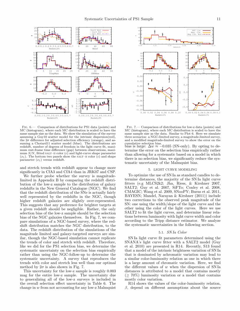
Fig. 6.— Comparison of distributions for PS1 data (points) andMC (histogram), where each MC distribution is scaled to have thesame sample size as the data. We show the simulation of the surveyassuming a Guy10 scatter model for the intrinsic dispersion(red),the 2σ difference for adjusted selection efficiency (orange), and as-suming a Chotard11 scatter model (blue). The distributions areredshift, number of degrees of freedom in the light curve fit, maxi-mum rest-frame time difference (gap) between observations, maxi-mum S/N , fitted salt–ii color (c) and light-curve shape parameter(x1). The bottom two panels show the salt–ii color (c) and shapeparameter (x1) versus redshift.

and stretch trends with redshift appear to change moresignificantly in CfA3 and CfA4 than in JRK07 and CSP.

We further probe whether the survey is magnitude-limited in Appendix B by comparing the redshift distri-bution of the low-z sample to the distribution of galaxyredshifts in the New General Catalogue (NGC). We findthat the redshift distribution of the SNe is actually fairlywell represented by the redshifts in the NGC, thoughhigher redshift galaxies are slightly over-represented.This suggests that any preference for brighter targets ata given redshift should be negligible. Rather, the onlyselection bias of the low-z sample should be the selectionbias of the NGC galaxies themselves. In Fig. 7, we com-pare simulations of a NGC-based survey, where the red-shift distribution matches the NGC distribution, to thedata. The redshift distribution of the simulations of themagnitude limited and galaxy-targeted surveys are sim-ilar, though the NGC-based simulation cannot replicatethe trends of color and stretch with redshift. Therefore,like we did for the PS1 selection bias, we determine thesystematic uncertainty on the selection bias empiricallyrather than using the NGC-follow-up to determine thesystematic uncertainty. A survey that reproduces thetrends with color and stretch less well than our optimalmethod by 2σ is also shown in Fig. 7.

This uncertainty for the low-z sample is roughly 0.003mag for the entire low-z sample. The uncertainty dueto generalizing all of the low-z surveys is included inthe overall selection effect uncertainty in Table 6. Thechange in w from not accounting for any low-z Malmquist

0.00 0.02 0.04 0.06 0.08 0.10

Redshift

0

20

40

60

80

100

#

NGC Lim.Mag. Lim.

Mag Lim. Mod

-0.2 0.0 0.2

c

010

20

30

40

50

60

#

-4 -2 0 2 4

x1

0

10

20

30

40

50

0.00 0.02 0.04 0.06 0.08 0.10

Redshift

-0.10

-0.08

-0.06

-0.04

-0.02

0.00

0.02

0.04

c

0.00 0.02 0.04 0.06 0.08 0.10

Redshift

-0.4

-0.2

0.0

0.2

0.4

x1

Fig. 7.— Comparison of distributions for low-z data (points) andMC (histogram), where each MC distribution is scaled to have thesame sample size as the data. Similar to Plot 6. Here we simulatethree scenarios: a NGC-limited survey, a magnitude-limited survey,and a modified magnitude-limited survey to show the error on thecumulative selection bias.bias is large: ∆w ≈ −0.035 (SN-only). By opting to de-termine the error on the selection bias empirically ratherthan allowing for a systematic based on a model in whichthere is no selection bias, we significantly reduce the sys-tematic uncertainty of the Malmquist bias.

5. LIGHT CURVE MODELING

To optimize the use of SN Ia as standard candles to de-termine distances, the majority of the SN Ia light curvefitters (e.g MLCS2k2; Jha, Riess, & Kirshner 2007,SALT2; Guy et al. 2007, SiFTo; Conley et al. 2008,CMAGIC; Wang et al. 2009, SNooPY; Burns et al. 2011,BAYESN; Mandel, Narayan & Kirshner (2011)) includetwo corrections to the observed peak magnitude of theSN: one using the width/slope of the light curve and theother using the color of the light curves. Here we useSALT2 to fit the light curves, and determine linear rela-tions between luminosity with light curve width and coloraccording to the Tripp distance estimator. We analyzethe systematic uncertainties in the following section.

5.1. SN Ia Color

SN Ia light curve fit parameters determined using theSNANA’s light curve fitter with a SALT2 model (Guyet al. 2010) are presented in R14. Recently, S13 foundthat a model of the intrinsic brightness variation of SN Iathat is dominated by achromatic variation may lead toa similar color-luminosity relation as one in which thereis a large amount of chromatic variation. Here, we findthe different values of w when the dispersion of SN Iadistances is attributed to a model that contains mostly(≥ 70%) luminosity variation or a model that containsmostly color variation.

R14 shows the values of the color-luminosity relation,β, depend on different assumptions about the source

12 Scolnic, Rest et al

of intrinsic scatter. They find that β = 3.10 ± 0.12when scatter is attributed to luminosity variation andβ = 3.86± 0.15 when scatter is attributed to color varia-tion. The latter value is only < 2σ from a MW-like red-dening law, though R14 notes this high value is stronglypulled by the low-z sample only. To understand the con-sequences of these two assumptions about intrinsic scat-ter, we first match simulations, as explained in the pre-vious section, of two variation models to the data. Wecreate simulations using SNANA with two models, onein which the majority of scatter is due to luminosity vari-ation (called ‘Guy10’, Guy et al. 2010, color/luminosityvariation - 30%/70%) and the other in which the ma-jority of scatter is due to color variation (called ‘Ch11’-Chotard 2011, color/luminosity variation - 75%/25%).For the model with a majority of luminosity variation,the color-luminosity relation, β is set to be 3.1, the valuefound after attributing all of the Hubble residual scat-ter to luminosity variation (R14). For the model withmostly color variation, SN Ia color is composed of a dustcomponent that correlates with luminosity via a Milky-Way-like reddening law (β = 4.1) and a variation compo-nent (Chotard 2011). SNANA provides these two mod-els. For Chotard (2011), SNANA converts a covariancematrix among bands into a model of SED variations. TheChotard (2011) model used is denoted ‘C110’ in SNANA.

S13 showed that trends in Hubble residuals versus colordepend not only on the intrinsic scatter but also theunderlying color distribution. Parameters for the un-derlying color and stretch distributions that best matchsimulations to the data are given in Table 4. These val-ues are found using a grid-based search of the x1 andc asymmetric gaussian parameters. S13 showed thatsimulations with a Guy10 variation model, combinedwith a slightly asymmetric underlying color distribution(Kessler et al. 2013), cannot reproduce the significantasymmetry around c ∼ −0.1 seen in the trends of Hub-ble residuals versus color (similarly shown for PS1+lzsample, given in Fig. 8 - top). Some correlation betweencolor and Hubble residuals should be expected from theTripp distance estimator, though the trend seen here canbe best explained by a narrow and asymmetric underly-ing color distribution (Table 4). To improve the con-sistency of the Guy10 model with observations, we findthat the underlying color distributions for this variationmodel should be significantly asymmetric. The distribu-tion presented here is much more asymmetric than thatgiven in Kessler et al. (2013) for the SDSS or SNLS sur-veys.

We present our distances biases with redshift in Fig. 9.Distances included here are found once intrinsic disper-sion of SN Ia is attributed to luminosity variation. Wefind differences in the distance corrections to be up to0.03 mag and note that the offsets are fairly constantwith redshift for the PS1 sample. We find overall a meanoffset of −0.01 mag for both models with the low-z sam-ple, and this offset is subtracted out from both the low-zand high-z samples as they are combined. This offset isdue to the asymmetric underlying color distribution andcovariances between mb and c. We further understandthe predictions by our two models by analyzing trendsbetween Hubble residual and color at separate redshiftbins in Fig. 10. While there are discrepancies in the pre-dictions for the two models of SN variation, the statistics

TABLE 4Asymmetric Gaussian parameters to describe the parent

distribution of x1 and c.

Parameter Sample Intr. Variation x σ− σ+

c PS1 Ch11 −0.1 0.0 0.095c PS1 Guy10 −0.08 0.04 0.13c Low-z Ch11 -0.09 0.0 0.12c Low-z Guy10 -0.05 0.04 0.13x1 PS1 Ch11 0.5 1.0 0.5x1 PS1 Guy10 -0.3 1.2 0.8x1 Low-z Ch11 0.5 1.0 0.5x1 Low-z Guy10 -0.3 1.2 0.8

Note. — The parameters defining the asymmetric Gaussian for

the color and light-curve shape distributions: e[−(x−x)2/2σ2−] for

x < x and e[−(x−x)2/2σ2+] for x > x. The optimized parameters

for the variation models with a majority due to color variation(Ch11-Chotard et al., color/luminosity variation - 75%/25%) andluminosity variation (Guy10-Guy et al., color/luminosity variation- 30%/70%) are given.

of the PS1+lz sample do not favor either model; the datacannot break the degeneracy. In Fig. 6, we also overplota simulation with our color variation model, and find nonoticeable differences from our simulation with luminos-ity variation.

Recent analyses (e.g., Campbell et al. 2013, Kessleret al. 2013) attempt to remove any fitter bias (includ-ing the Malmquist bias) by using simulations to find themean distance residual for a given redshift, like the oneswe have done here. We may use our two different sim-ulations to find the systematic uncertainty in our dis-tance corrections from our incomplete understanding ofthe true variation model. For our primary analysis, wecorrect for the average distance residual at all redshiftsfrom the two simulations. These average distance resid-uals are shown in Fig. 9. The difference in w after ap-plying the corrections from one model or the other is∆w ≈ 0.055 (Lum.-Col.). By taking the average, we re-duce the systematic uncertainty due to the color modelsby a factor of 2.

A separate way to determine the systematic uncer-tainty from SN color is to compare the values of w whenusing SALT2 in the conventional manner (attribute in-trinsic scatter to luminosity variation) as well as usingBaSALT (S13), a Bayesian approach that separates thecolor of each SN into components of color variation anddust. To retrieve the component of color that correlateswith luminosity (cdust), BaSALT applies a Bayesian priorto the observed color (cobs) such that

cdust =1

P

∫c>c

ce−(c−cobs)/2σ2cn e−(c−c)2/τS(z)2∂c. (7)

Here, cn is the noise from the color measurement and Pis a normalization constant. The second part of Eqn. 7describes the Bayesian prior (Riess, Press, & Kirshner1996) for the dust distribution where c is the blue cutoffof the distribution. τS(z) describes the shape of the onesided Gaussian due to extinction for a given redshift z foreach survey S; the dependence of τ on survey and redshiftallows selection effects to be modeled. As discussed in theprevious section, for the low-z sample we do not expectselection effects to significantly vary with redshift and

Systematic Uncertainties of PS1 Sample 13

-0.4

-0.2

0.0

0.2

0.4

SALT2

-0.2 -0.1 0.0 0.1 0.2

c

-0.4

-0.2

0.0

0.2

0.4

BaSALT

µ -

µ

Λ CDM (mag)

Fig. 8.— Hubble Residuals versus color for the SALT2 (top) andBaSALT (bottom) methods over the entire redshift range.

therefore we do not change τ with redshift. For the PS1sample, however, τ varies with redshift27. The results areshown in Fig. 8 (bottom). The BaSALT method does notallow the color fits to be bluer than c = −0.1 and there-fore the particular non-linearity between Hubble resid-ual and color is much weaker with this method. How-ever, given the BaSALT method, we introduce with thecolor prior additional correlations between color and dis-tance that are dependent on the uncertainty of the prior.Therefore, we only use the BaSALT method as a wayto confirm our results using the simulations discussedabove. We find a change in w of ∆w = wB−wS = −0.06when the BaSALT method is used instead of the SALT2method. This is nearly equal to the difference found forw from using distance corrections from simulations of thedifferent scatter models. With the BaSALT method, westill must use simulations to correct for any further bi-ases due to covariances between color and the other lightcurve fit parameters. If information about the underly-ing color distribution was included during the light curvefit itself, this would not be needed.

The difference in recovered cosmological parametersdue to variation models largely depends on the meancolor of the sample. If the mean color of the sample isconstant with redshift, we should not expect significant(|∆w| > 0.01) discrepancies due to finding the wrong β.In the PS1+lz sample, the PS1 subsample is bluer by∼ 0.03 mag than the low-z sample, and thus the effect ofan incorrect β is significant.

5.2. Non-linear Light-curve Shape

We now explore whether the relation between the light-curve shape and luminosity is adequately described bya linear model. Similar to the analysis of color, we ob-serve the trend between Hubble residuals and light-curve

27 For Low-z: τ = 0.11. For PS1: τ = [0.11, 0.10, 0.08, 0.06] for~z = [0.1, 0.3, 0.5, 0.7].

0.00 0.02 0.04 0.06 0.08 0.10

-0.10

-0.08

-0.06

-0.04

-0.02

0.00

0.02

0.04

0.0 0.1 0.2 0.3 0.4 0.5 0.6 0.7

-0.10

-0.08

-0.06

-0.04

-0.02

0.00

0.02

0.04

Avg. Dist. BiasCh11Guy10

µ -

µSim. (mag)

z

Fig. 9.— The distance biases over the entire redshift range for ourtwo variation models. The average of these biases is also shown.The inner errors show the errors from the simulation, whereas theouter errors include this error as well as the error in the selectionbias uncertainty.

shape, known in SALT2 as ‘stretch’ (x1). Doing so, wefind that a second-order polynomial (α1 × x1 + α2 × x2

1,where [a1, a2] = [0.160 ± 0.010, 0.017 ± 0.007]) appearsto better fit the data than the conventional linear model(α×x1). The reduction in χ2 when including the secondorder is from 312 to 301.8 for 312 SNe (after uncertaintieshave been inflated such that χ2

ν = 1 and not includingthe α2 term in the uncertainty). The significance foundhere is larger than that found in Sullivan et al. 2010 orSullivan et al. 2011 when they examine a second orderstretch correction. In the Sullivan et al. papers, theyfind two α values for high and low-stretch values, bothof which were larger than the value of α found for thewhole sample. We find a discrepancy in Hubble residualsfor high (x1 > 0.5) and low stretch (x1 < 0.5) values tobe ∆µ = 0.042± 0.020 (after Malmquist correction).

A more practical approach to understand the source ofthe second-order trend of Hubble residuals with stretch isto reproduce the observed effect in simulations. We find(Fig. 11) that the trend seen in the data may be repli-cated with two different α parameters for high (x1 > 0)and low (x1 < 0) stretch values. We use this split func-tion as we do not yet have the tools to simulate a sec-ond order polynomial of the stretch-luminosity relation.A comparison of results of various simulations with thedata is presented in Fig. 11. We show that the quadratictrend between Hubble residuals and stretch that is seenin the data is not seen in simulations with only one α(α = 0.14). However, for the 2α model, where for x1 < 0,α = 0.08 and for x1 > 0, α = 0.17, the quadratic trendis observed. More work must be done to determine ifthis effect is real, and if a continuous, but non-linear,Phillips relation is empirically favorable to the discon-tinuous relation presented here. We find the change inthe determined value of w when accounting for a second-

14 Scolnic, Rest et al

-0.4

-0.2

0.0

0.2

0.4

∆ µ= -0.011

∆ µ= -0.006

µ (

β=3.1,

α=0.14) -

µ Λ CDM (mag) 0.0 < z < 0.15

∆ µ= -0.034

∆ µ= -0.006

0.15 < z < 0.30

-0.2 -0.1 0.0 0.1 0.2c

-0.4

-0.2

0.0

0.2

0.4

∆ µ= -0.039

∆ µ= -0.013

PS1+lowz Data

0.30 < z < 0.45

-0.2 -0.1 0.0 0.1 0.2c

∆ µ= -0.059

∆ µ= -0.036

Guy10 Beta=3.1C11 Beta=4.1

0.45 < z

Fig. 10.— Hubble Residuals as a function of color for differentredshift bins. Distances are found using the conventional SALT2method where residual scatter is attributed to luminosity variation.One simulation is in accordance with the conventional SALT2 as-sumptions, whereas the other simulation follows the color variationmodel (BaSALT). The lowest redshift bin contains all of the Nearbysupernovae.

order light-curve shape correction is small: ∆w = +0.01.Since there is only mild evidence (∼ 2σ) that a second-order light curve shape correction is beneficial, it is notincluded in our overall uncertainty budget.

5.3. Host Galaxy Dependence

We examine here whether Hubble residuals of the SNein the PS1+low-z sample correlate with properties of thehost galaxies of SNe. These correlations have been shownfor other SN Ia samples in multiple recent studies (e.g.,Kelly et al. 2010, Sullivan et al. 2010a, Lampeitl et al.2010). While age, metallicity, and Star-Formation-Rate(SFR) of host galaxies all also have been observed tocorrelate with Hubble Residuals (e.g., Gupta et al. 2011,Hayden et al. 2013), here we focus on the masses of thehost galaxies.

To determine the masses of host galaxies of PS1SN Ia, we combine PS1 observations with u band datafrom SDSS. Since the PS1 Medium Deep Survey hasnow observed each of the SN Ia host galaxies for overtwo years, we stacked deep (SNR of 10 at rp1 ∼ 24)SN-free templates and used SExtractor’s FLUX AUTO(Bertin & Arnouts 1996) to determine the flux valuesin gp1,rp1,ip1,zp1,yp1. The measured magnitudes are an-alyzed with the SED fitting software Multi-wavelengthAnalysis of Galaxy Physical Properties (da Cunha et al.2011) to calculate the stellar masses of host galaxies.To verify both our galaxy photometry and the mass fit-

-2 -1 0 1 2

x1

-0.2

0.0

0.2

µ -

µLCDM

Data Fit

Sim: 1 α

Sim: 2 α

Fig. 11.— Hubble Residuals versus stretch for the PS1+lz dataand simulations. The results for simulations are from a 1 α and 2α model.

ting routine, we ran our mass fitter on PS1 photome-try of host galaxies in the Gupta et al. (2011) sample,and found differences with Gupta et al. (2011) to be< log(M) ∼ 0.05.

The mass distributions of the host galaxies from thecombined PS1+low-z sample analyzed for this paper areshown in Fig. 12. We currently have masses for 110 ofthe 113 PS1 host galaxies and 61 of the 197 low-z hostgalaxies. The host galaxy masses of the low-z sampleare from Sullivan et al. (2010a) and the incompletenesslimits a full analysis. Because most low-z supernovaewere found in catalogued galaxies, and catalogued galax-ies are generally brighter and more massive on average,the host galaxies in the low-z surveys are log(M) ∼ 0.5more massive than those in the PS1 survey. We find fromFig. 13 a trend such that supernovae with more massivehost galaxies have lower stretch values, though quanti-fying this trend is obscured by a number of supernovaewith very low stretch errors (dx1 < 0.1). We find a re-lation between Hubble residual and color with a slope of0.0054 ± 0.0049. While the significance of this relationis weak, it is in agreement with the trend observed byChildress et al. (2013).

In Fig. 14, we show the trend between Hubble resid-uals and the host galaxy mass. We find a step-size inHubble residuals, for a mass split of log(M) = 10, of∆µ = 0.037 ± 0.032 mags. While this is consistent withthe step-size seen in previous studies (∼ 0.08 mag; e.g.,Sullivan et al. 2010a, Gupta et al. 2011), it is also con-sistent with zero. For the PS1 SNe alone, we find only adifference of 0.019± 0.025, weaker than the typical valueseen. Part of the impact of adding in the low-z sam-ple may be due to the fact that low-z hosts have highermasses, on average, than high-z hosts. Therefore, anydifference in luminosity is degenerate with discrepanciesin calibration for the low-z and high-z samples. It is alsopossible that the low value of intrinsic scatter seen in

Systematic Uncertainties of PS1 Sample 15

the PS1 sample (σint = 0.07) found for the PS1 sam-ple is related to the low significance of the host galaxyrelation. One concern is that the mass fits are likely sub-ject to selection biases as the number of observations inseparate filters decreases at higher redshift, (e.g., Galexand UKIDSS detect more nearby hosts). However, Smithet al. (2012) finds discrepancies in the determination ofmass for SNe with high and low redshift to be negligiblefor the SDSS+SNLS sample.

As we do not understand why the difference in lumi-nosity between low and high-mass galaxies is weaker inthe PS1+lz sample than in other samples, we includeas a systematic uncertainty the possibility that the hostgalaxy relation is as seen in other surveys (e.g. Childresset al. 2013) versus the size seen in our sample. We imple-ment for the PS1 sample the same mass-distribution splitdone in Sullivan et al. (2010a) at (log(M) = 10) andapply a difference in luminosities between SNe with highand low massive host galaxies at ∼ 0.075 mag (Sullivanet al. 2010a). When we do not have sufficient host galaxyphotometry to find masses, we do not correct the SN dis-tance. If, however, the host is not visible, we assume themass is low. We find that the correction based on hostgalaxy masses changes our value of w by ∆w = 0.026(SN+BAO+CMB+H0: host correction - no-host correc-tion). The overall uncertainty for the host galaxy cor-rection is shown in Table 6. Its effect on the recovery ofcosmological parameters is not as large as some of theother uncertainties, which may be partly due to the in-completeness of host galaxy measurements for the low-zsample.

7 8 9 10 11 12

PS1 Host Galaxy Mass

0

2

4

6

8

10

12

#

PS1Low-z

Fig. 12.— The host galaxy mass distribution for the PS1 sampleand combined low-z sample.

6. REDSHIFT UNCERTAINTIES

Inhomogeneities in the density field generate peculiarvelocities that perturb the Hubble flow (see Strauss &Willick 1995 for a review). The overall uncertainty in

-0.3

-0.2

-0.1

-0.0

0.1

0.2

0.3

c

7 8 9 10 11 12

Host Galaxy Mass

-3

-2

-1

0

1

2

3

x1

Fig. 13.— The SALT2 stretch parameter x1 and color c as afunction of the host galaxy Mstellar for the entire PS1 sample.The red points show the weighted means.

7 8 9 10 11 12

Host Galaxy Mass

-0.4

-0.2

0.0

0.2

0.4

µ-

µBest (Mags)

Low M_S

High M_S

Fig. 14.— Residuals from the best-fitting cosmology for PS1 as afunction of host galaxy Mstellar. The red points show the weightedmean residuals in bins of host Mstellar

redshift for each SN can be expressed as:

σ2z = σ2

z,spec + σ2z,flow. (8)

where σz,spec is the spectroscopic uncertainty and σz,flowis the correlated velocity uncertainty of SN peculiar ve-locities relative to the Hubble flow.

These uncertainties propagate towards an uncertainty

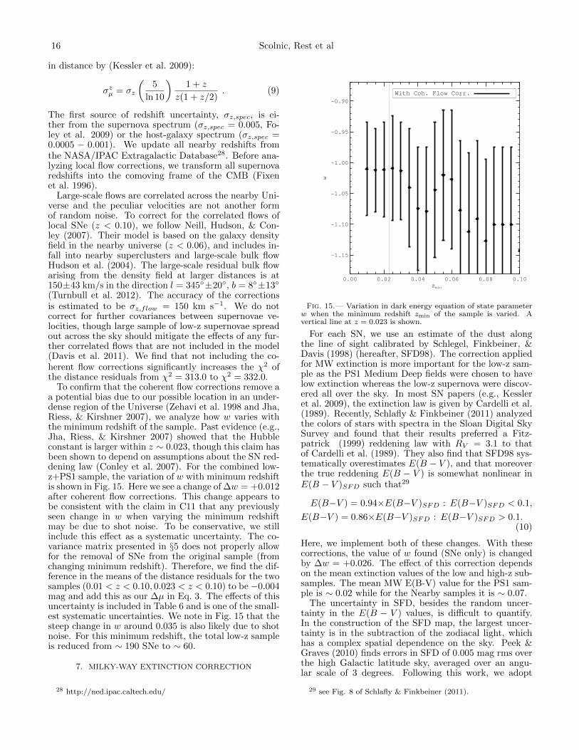
16 Scolnic, Rest et al

in distance by (Kessler et al. 2009):

σzµ = σz

(5

ln 10

)1 + z

z(1 + z/2). (9)

The first source of redshift uncertainty, σz,spec, is ei-ther from the supernova spectrum (σz,spec = 0.005, Fo-ley et al. 2009) or the host-galaxy spectrum (σz,spec =0.0005 − 0.001). We update all nearby redshifts fromthe NASA/IPAC Extragalactic Database28. Before ana-lyzing local flow corrections, we transform all supernovaredshifts into the comoving frame of the CMB (Fixenet al. 1996).

Large-scale flows are correlated across the nearby Uni-verse and the peculiar velocities are not another formof random noise. To correct for the correlated flows oflocal SNe (z < 0.10), we follow Neill, Hudson, & Con-ley (2007). Their model is based on the galaxy densityfield in the nearby universe (z < 0.06), and includes in-fall into nearby superclusters and large-scale bulk flowHudson et al. (2004). The large-scale residual bulk flowarising from the density field at larger distances is at150±43 km/s in the direction l = 345±20, b = 8±13

(Turnbull et al. 2012). The accuracy of the correctionsis estimated to be σz,flow = 150 km s−1. We do notcorrect for further covariances between supernovae ve-locities, though large sample of low-z supernovae spreadout across the sky should mitigate the effects of any fur-ther correlated flows that are not included in the model(Davis et al. 2011). We find that not including the co-herent flow corrections significantly increases the χ2 ofthe distance residuals from χ2 = 313.0 to χ2 = 332.0.

To confirm that the coherent flow corrections remove aa potential bias due to our possible location in an under-dense region of the Universe (Zehavi et al. 1998 and Jha,Riess, & Kirshner 2007), we analyze how w varies withthe minimum redshift of the sample. Past evidence (e.g.,Jha, Riess, & Kirshner 2007) showed that the Hubbleconstant is larger within z ∼ 0.023, though this claim hasbeen shown to depend on assumptions about the SN red-dening law (Conley et al. 2007). For the combined low-z+PS1 sample, the variation of w with minimum redshiftis shown in Fig. 15. Here we see a change of ∆w = +0.012after coherent flow corrections. This change appears tobe consistent with the claim in C11 that any previouslyseen change in w when varying the minimum redshiftmay be due to shot noise. To be conservative, we stillinclude this effect as a systematic uncertainty. The co-variance matrix presented in §5 does not properly allowfor the removal of SNe from the original sample (fromchanging minimum redshift). Therefore, we find the dif-ference in the means of the distance residuals for the twosamples (0.01 < z < 0.10, 0.023 < z < 0.10) to be −0.004mag and add this as our ∆µ in Eq. 3. The effects of thisuncertainty is included in Table 6 and is one of the small-est systematic uncertainties. We note in Fig. 15 that thesteep change in w around 0.035 is also likely due to shotnoise. For this minimum redshift, the total low-z sampleis reduced from ∼ 190 SNe to ∼ 60.

7. MILKY-WAY EXTINCTION CORRECTION

28 http://ned.ipac.caltech.edu/

0.00 0.02 0.04 0.06 0.08 0.10

zmin

-1.15

-1.10

-1.05

-1.00

-0.95

-0.90

w

With Coh. Flow Corr.

Fig. 15.— Variation in dark energy equation of state parameterw when the minimum redshift zmin of the sample is varied. Avertical line at z = 0.023 is shown.

For each SN, we use an estimate of the dust alongthe line of sight calibrated by Schlegel, Finkbeiner, &Davis (1998) (hereafter, SFD98). The correction appliedfor MW extinction is more important for the low-z sam-ple as the PS1 Medium Deep fields were chosen to havelow extinction whereas the low-z supernova were discov-ered all over the sky. In most SN papers (e.g., Kessleret al. 2009), the extinction law is given by Cardelli et al.(1989). Recently, Schlafly & Finkbeiner (2011) analyzedthe colors of stars with spectra in the Sloan Digital SkySurvey and found that their results preferred a Fitz-patrick (1999) reddening law with RV = 3.1 to thatof Cardelli et al. (1989). They also find that SFD98 sys-tematically overestimates E(B − V ), and that moreoverthe true reddening E(B − V ) is somewhat nonlinear inE(B − V )SFD such that29

E(B−V ) = 0.94×E(B−V )SFD : E(B−V )SFD < 0.1,

E(B−V ) = 0.86×E(B−V )SFD : E(B−V )SFD > 0.1.(10)

Here, we implement both of these changes. With thesecorrections, the value of w found (SNe only) is changedby ∆w = +0.026. The effect of this correction dependson the mean extinction values of the low and high-z sub-samples. The mean MW E(B-V) value for the PS1 sam-ple is ∼ 0.02 while for the Nearby samples it is ∼ 0.07.

The uncertainty in SFD, besides the random uncer-tainty in the E(B − V ) values, is difficult to quantify.In the construction of the SFD map, the largest uncer-tainty is in the subtraction of the zodiacal light, whichhas a complex spatial dependence on the sky. Peek &Graves (2010) finds errors in SFD of 0.005 mag rms overthe high Galactic latitude sky, averaged over an angu-lar scale of 3 degrees. Following this work, we adopt

29 see Fig. 8 of Schlafly & Finkbeiner (2011).

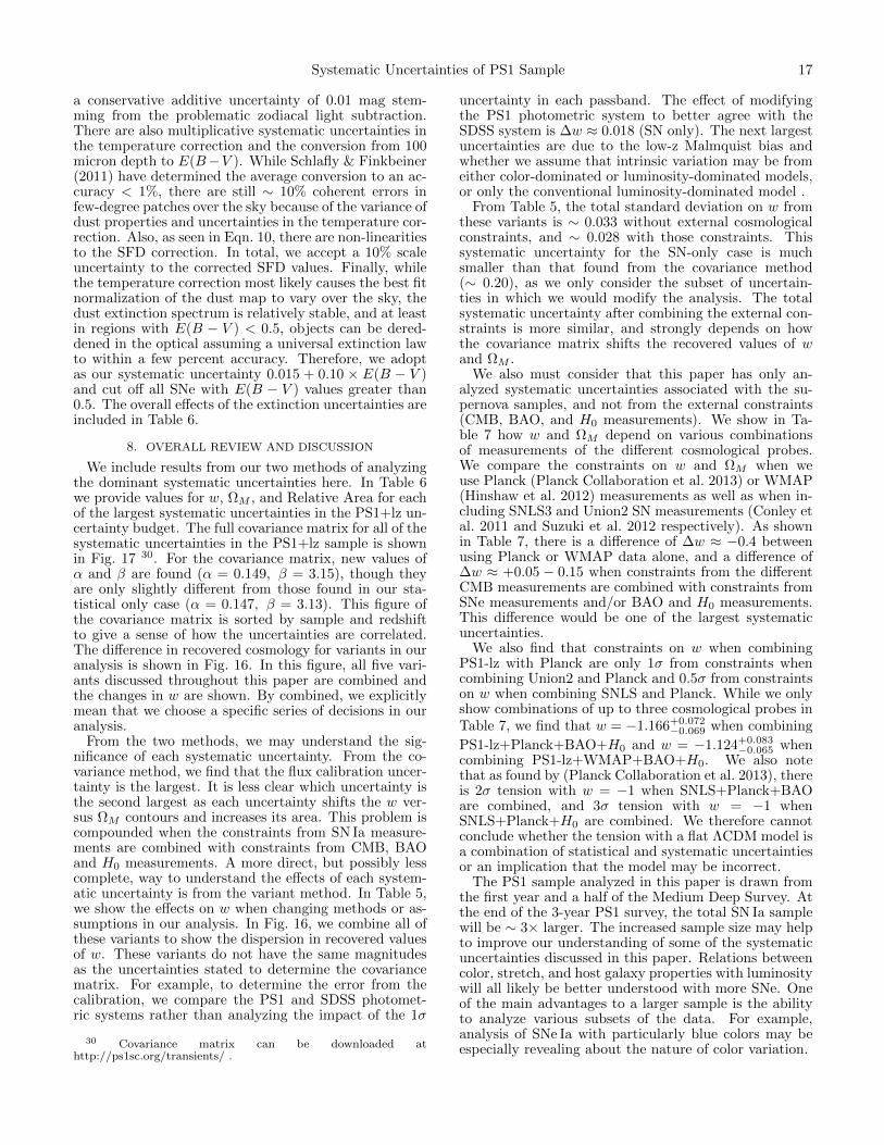
Systematic Uncertainties of PS1 Sample 17

a conservative additive uncertainty of 0.01 mag stem-ming from the problematic zodiacal light subtraction.There are also multiplicative systematic uncertainties inthe temperature correction and the conversion from 100micron depth to E(B−V ). While Schlafly & Finkbeiner(2011) have determined the average conversion to an ac-curacy < 1%, there are still ∼ 10% coherent errors infew-degree patches over the sky because of the variance ofdust properties and uncertainties in the temperature cor-rection. Also, as seen in Eqn. 10, there are non-linearitiesto the SFD correction. In total, we accept a 10% scaleuncertainty to the corrected SFD values. Finally, whilethe temperature correction most likely causes the best fitnormalization of the dust map to vary over the sky, thedust extinction spectrum is relatively stable, and at leastin regions with E(B − V ) < 0.5, objects can be dered-dened in the optical assuming a universal extinction lawto within a few percent accuracy. Therefore, we adoptas our systematic uncertainty 0.015 + 0.10 × E(B − V )and cut off all SNe with E(B − V ) values greater than0.5. The overall effects of the extinction uncertainties areincluded in Table 6.

8. OVERALL REVIEW AND DISCUSSION

We include results from our two methods of analyzingthe dominant systematic uncertainties here. In Table 6we provide values for w, ΩM , and Relative Area for eachof the largest systematic uncertainties in the PS1+lz un-certainty budget. The full covariance matrix for all of thesystematic uncertainties in the PS1+lz sample is shownin Fig. 17 30. For the covariance matrix, new values ofα and β are found (α = 0.149, β = 3.15), though theyare only slightly different from those found in our sta-tistical only case (α = 0.147, β = 3.13). This figure ofthe covariance matrix is sorted by sample and redshiftto give a sense of how the uncertainties are correlated.The difference in recovered cosmology for variants in ouranalysis is shown in Fig. 16. In this figure, all five vari-ants discussed throughout this paper are combined andthe changes in w are shown. By combined, we explicitlymean that we choose a specific series of decisions in ouranalysis.

From the two methods, we may understand the sig-nificance of each systematic uncertainty. From the co-variance method, we find that the flux calibration uncer-tainty is the largest. It is less clear which uncertainty isthe second largest as each uncertainty shifts the w ver-sus ΩM contours and increases its area. This problem iscompounded when the constraints from SN Ia measure-ments are combined with constraints from CMB, BAOand H0 measurements. A more direct, but possibly lesscomplete, way to understand the effects of each system-atic uncertainty is from the variant method. In Table 5,we show the effects on w when changing methods or as-sumptions in our analysis. In Fig. 16, we combine all ofthese variants to show the dispersion in recovered valuesof w. These variants do not have the same magnitudesas the uncertainties stated to determine the covariancematrix. For example, to determine the error from thecalibration, we compare the PS1 and SDSS photomet-ric systems rather than analyzing the impact of the 1σ

30 Covariance matrix can be downloaded athttp://ps1sc.org/transients/ .

uncertainty in each passband. The effect of modifyingthe PS1 photometric system to better agree with theSDSS system is ∆w ≈ 0.018 (SN only). The next largestuncertainties are due to the low-z Malmquist bias andwhether we assume that intrinsic variation may be fromeither color-dominated or luminosity-dominated models,or only the conventional luminosity-dominated model .

From Table 5, the total standard deviation on w fromthese variants is ∼ 0.033 without external cosmologicalconstraints, and ∼ 0.028 with those constraints. Thissystematic uncertainty for the SN-only case is muchsmaller than that found from the covariance method(∼ 0.20), as we only consider the subset of uncertain-ties in which we would modify the analysis. The totalsystematic uncertainty after combining the external con-straints is more similar, and strongly depends on howthe covariance matrix shifts the recovered values of wand ΩM .

We also must consider that this paper has only an-alyzed systematic uncertainties associated with the su-pernova samples, and not from the external constraints(CMB, BAO, and H0 measurements). We show in Ta-ble 7 how w and ΩM depend on various combinationsof measurements of the different cosmological probes.We compare the constraints on w and ΩM when weuse Planck (Planck Collaboration et al. 2013) or WMAP(Hinshaw et al. 2012) measurements as well as when in-cluding SNLS3 and Union2 SN measurements (Conley etal. 2011 and Suzuki et al. 2012 respectively). As shownin Table 7, there is a difference of ∆w ≈ −0.4 betweenusing Planck or WMAP data alone, and a difference of∆w ≈ +0.05 − 0.15 when constraints from the differentCMB measurements are combined with constraints fromSNe measurements and/or BAO and H0 measurements.This difference would be one of the largest systematicuncertainties.

We also find that constraints on w when combiningPS1-lz with Planck are only 1σ from constraints whencombining Union2 and Planck and 0.5σ from constraintson w when combining SNLS and Planck. While we onlyshow combinations of up to three cosmological probes inTable 7, we find that w = −1.166+0.072

−0.069 when combining

PS1-lz+Planck+BAO+H0 and w = −1.124+0.083−0.065 when

combining PS1-lz+WMAP+BAO+H0. We also notethat as found by (Planck Collaboration et al. 2013), thereis 2σ tension with w = −1 when SNLS+Planck+BAOare combined, and 3σ tension with w = −1 whenSNLS+Planck+H0 are combined. We therefore cannotconclude whether the tension with a flat ΛCDM model isa combination of statistical and systematic uncertaintiesor an implication that the model may be incorrect.

The PS1 sample analyzed in this paper is drawn fromthe first year and a half of the Medium Deep Survey. Atthe end of the 3-year PS1 survey, the total SN Ia samplewill be ∼ 3× larger. The increased sample size may helpto improve our understanding of some of the systematicuncertainties discussed in this paper. Relations betweencolor, stretch, and host galaxy properties with luminositywill all likely be better understood with more SNe. Oneof the main advantages to a larger sample is the abilityto analyze various subsets of the data. For example,analysis of SNe Ia with particularly blue colors may beespecially revealing about the nature of color variation.

18 Scolnic, Rest et al

TABLE 5Variants in Analysis Relative to primary Method

Variant ∆ΩM ∆w ∆ΩM (+Ext.) ∆w (Ext.)

Nominal: 0.0 (0.217) 0.0 (-1.010) 0.0 (0.284) 0.0 (-1.131)Calib (PS1* vs PS1-SDSS): -0.013 0.018 -0.001 -0.006Intrinsic Variation (Color/Lum.* vs. Lum.): -0.005 0.044 0.005 0.027zmin (0.01* vs. 0.023): 0.001 0.013 0.002 0.011Low-z Malmquist (Yes* vs. No): -0.007 0.023 0.001 0.006Host Gal. Corr. (No* vs Yes): 0.016 0.003 0.006 0.026

Note. — The retrieved cosmology (SN only) for variants in the analysis relative to our primary method. The variants are: Calibration(PS1* or the SDSS modification of PS1), variation model (the average of the models with Ch11 or Guy10 scatter* or only the one withGuy10 scatter model), minimum redshift (z = 0.01* or z = 0.023), whether a low-z Malmquist correction is applied (Yes* or No) andwhether a correction to distances based on host galaxy masses is applied (No* or Yes). Asterisk implies primary method. Values given aree.g. w+V ariant−wPrimary . For the effects on w from each variant shown here, all other variants follow the primary method. Combinationsof these variants are shown in Fig. 16.

TABLE 6Overall Systematics

Systematic ∆ΩM ∆w Rel.area ∆ΩM ∆w Rel. areaSN Only SN+BAO+CMB+H0

Stat. Only 0.000 0.000 1.000 0.010 0.000 1.000(ΩM = 0.223+0.209

−0.221) (w = −1.010+0.360−0.206) (ΩM = 0.284+0.010

−0.010) (w = −1.131+0.049−0.049)

Calibration 0.024 -0.093 1.566 0.006 -0.035 1.309Color Model 0.004 -0.023 1.117 0.009 -0.012 1.106Host Gal. 0.006 0.000 1.035 0.011 0.006 0.977Malmquist 0.004 -0.011 1.024 0.010 -0.002 1.015zmin 0.000 -0.004 1.020 0.010 -0.003 1.023MW Extinction 0.001 -0.007 1.020 0.010 -0.004 1.019

Syst.+Stat. 0.032 -0.108 1.697 0.006 -0.035 1.333(ΩM = 0.256+0.201

−0.174) (w = −1.120+0.450−0.357) (ΩM = 0.280+0.013

−0.012) (w = −1.166+0.072−0.069)

Note. — The dominant systematic uncertainties in the PS1+lz sample with respect to Ωm and w. Ωm and w are given for a flatuniverse and ∆Ωm and ∆w values are the relative values such that, e.g. wstat+sys − wstat. Individual systematic uncertainties for eachof the PS1 passbands as well as the systematic uncertainties for each low-z sample. RelativeArea is the size of the contour that encloses68.3% of the probability distribution between w and ΩM compared with that of statistical only uncertainties.

To reduce the other systematic uncertainties, externaldata to the Medium Deep Survey will be needed. Forabsolute calibration, there is still room for improvementby including more Calspec standards, particularly thosethat are covered by multiple surveys so that full com-parisons can be done between the surveys. This analysiswill improve the accuracy in which PS1 is included intoa larger sample. Another promising development in thenext year is better absolute calibration of Calspec stan-dards (Kaiser et al. in prep).

In this paper, we have modeled the selection effects ofthe PS1 survey as well as the other low-z surveys. Asmore samples are combined to make one large, ‘Union’-like compilation, it is imperative that selection effectsare publicized and standardized. For a survey like PS1,where spectroscopic selection may have a degree of ran-domness, selection modeling may be inherently difficult.We have shown here one method to analyze selectioneffects without an underlying knowledge of the spectro-scopic follow-up program. This method may be used forany survey, though it is possible that the method mayyield biases if spectroscopic follow-up has distinct pro-grams.

There are other uncertainties we do not include in thisanalysis. Gravitational lensing may affect the appar-ent brightness of our supernovae, as the brightness maychange via amplification or de-amplification. There is aredshift-dependent additional scatter due to this ampli-fication of σµ−lens = 0.055z (Jonsson et al. 2010). Forthe SN Ia included in our sample, this additional uncer-tainty is dominated by photometric errors and needs tobe better understood.

The impact of the systematic uncertainties in thePS1+lz analysis on constraints of w are similar to thosepresented by C11 and Sullivan et al. (2011) for theSNLS3+SDSS+low-z sample. While their sample sizeis 472 compared to our 313, and they have many morehigher-z objects from SNLS and HST, the relative area oftheir ΩM versus w constraints when including all of thesystematic uncertainties is 1.85 compared to our 1.697.Their systematic uncertainties are mostly dominated bycalibration (relative area is 1.79 of total 1.85) while oursis 1.57 out of 1.70. Part of the small difference in thiscomparison is due to our larger estimates of the uncer-tainties in the underlying color model. Uncertainties dueto the minimum redshift of the sample are not included in

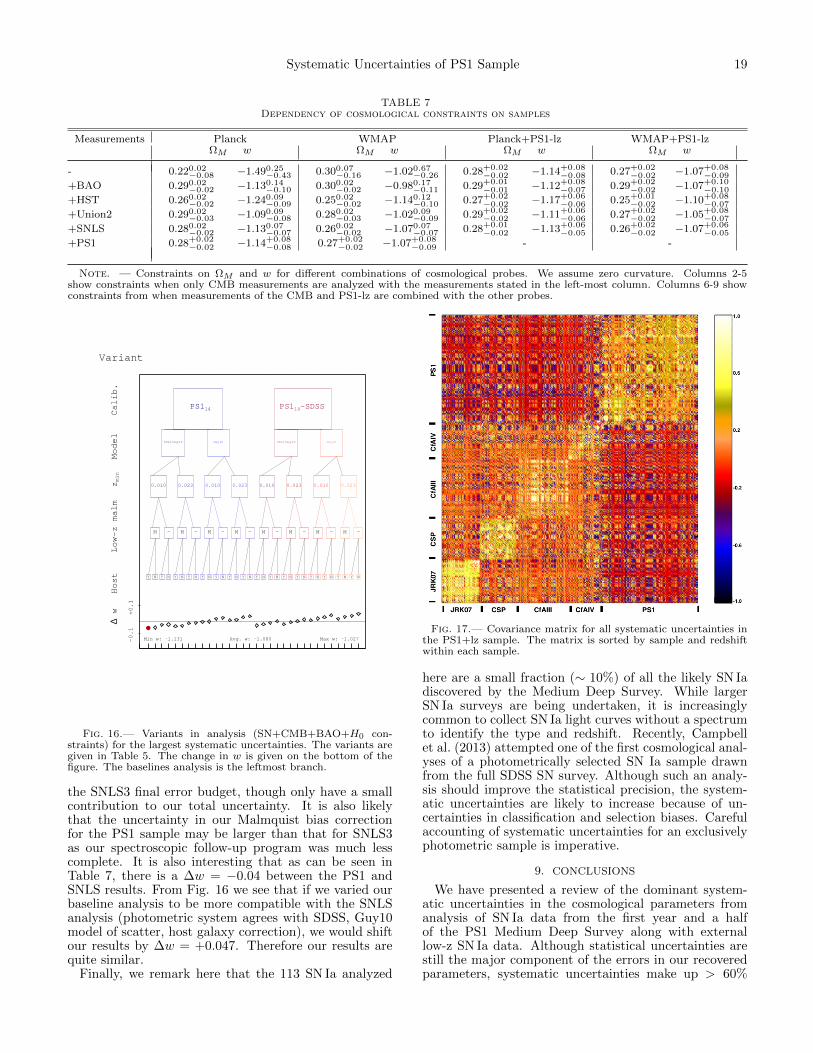
Systematic Uncertainties of PS1 Sample 19

TABLE 7Dependency of cosmological constraints on samples

Measurements Planck WMAP Planck+PS1-lz WMAP+PS1-lzΩM w ΩM w ΩM w ΩM w

- 0.220.02−0.08 −1.490.25

−0.43 0.300.07−0.16 −1.020.67

−0.26 0.28+0.02−0.02 −1.14+0.08

−0.08 0.27+0.02−0.02 −1.07+0.08

−0.09

+BAO 0.290.02−0.02 −1.130.14

−0.10 0.300.02−0.02 −0.980.17

−0.11 0.29+0.01−0.01 −1.12+0.08

−0.07 0.29+0.02−0.02 −1.07+0.10

−0.10

+HST 0.260.02−0.02 −1.240.09

−0.09 0.250.02−0.02 −1.140.12

−0.10 0.27+0.02−0.02 −1.17+0.06

−0.06 0.25+0.01−0.02 −1.10+0.08

−0.07

+Union2 0.290.02−0.03 −1.090.09

−0.08 0.280.02−0.03 −1.020.09

−0.09 0.29+0.02−0.02 −1.11+0.06

−0.06 0.27+0.02−0.02 −1.05+0.08

−0.07

+SNLS 0.280.02−0.02 −1.130.07

−0.07 0.260.02−0.02 −1.070.07

−0.07 0.28+0.01−0.02 −1.13+0.06

−0.05 0.26+0.02−0.02 −1.07+0.06

−0.05

+PS1 0.28+0.02−0.02 −1.14+0.08

−0.08 0.27+0.02−0.02 −1.07+0.08

−0.09 - -

Note. — Constraints on ΩM and w for different combinations of cosmological probes. We assume zero curvature. Columns 2-5show constraints when only CMB measurements are analyzed with the measurements stated in the left-most column. Columns 6-9 showconstraints from when measurements of the CMB and PS1-lz are combined with the other probes.

Calib.

Variant

PS114 PS114-SDSS

Model

Ch11/Guy10 Guy10 Ch11/Guy10 Guy10

zmin

0.010 0.023 0.010 0.023 0.010 0.023 0.010 0.023

Low-z malm

M - M - M - M - M - M - M - M -

Host Y N Y N Y N Y N Y N Y N Y N Y N Y N Y N Y N Y N Y N Y N Y N Y N

∆

w

Min w: -1.131 Avg. w: -1.080 Max w: -1.027

+0.1

-0.1

-

-

Fig. 16.— Variants in analysis (SN+CMB+BAO+H0 con-straints) for the largest systematic uncertainties. The variants aregiven in Table 5. The change in w is given on the bottom of thefigure. The baselines analysis is the leftmost branch.

the SNLS3 final error budget, though only have a smallcontribution to our total uncertainty. It is also likelythat the uncertainty in our Malmquist bias correctionfor the PS1 sample may be larger than that for SNLS3as our spectroscopic follow-up program was much lesscomplete. It is also interesting that as can be seen inTable 7, there is a ∆w = −0.04 between the PS1 andSNLS results. From Fig. 16 we see that if we varied ourbaseline analysis to be more compatible with the SNLSanalysis (photometric system agrees with SDSS, Guy10model of scatter, host galaxy correction), we would shiftour results by ∆w = +0.047. Therefore our results arequite similar.

Finally, we remark here that the 113 SN Ia analyzed

Fig. 17.— Covariance matrix for all systematic uncertainties inthe PS1+lz sample. The matrix is sorted by sample and redshiftwithin each sample.

here are a small fraction (∼ 10%) of all the likely SN Iadiscovered by the Medium Deep Survey. While largerSN Ia surveys are being undertaken, it is increasinglycommon to collect SN Ia light curves without a spectrumto identify the type and redshift. Recently, Campbellet al. (2013) attempted one of the first cosmological anal-yses of a photometrically selected SN Ia sample drawnfrom the full SDSS SN survey. Although such an analy-sis should improve the statistical precision, the system-atic uncertainties are likely to increase because of un-certainties in classification and selection biases. Carefulaccounting of systematic uncertainties for an exclusivelyphotometric sample is imperative.

9. CONCLUSIONS

We have presented a review of the dominant system-atic uncertainties in the cosmological parameters fromanalysis of SN Ia data from the first year and a halfof the PS1 Medium Deep Survey along with externallow-z SN Ia data. Although statistical uncertainties arestill the major component of the errors in our recoveredparameters, systematic uncertainties make up > 60%

20 Scolnic, Rest et al

0.0 0.2 0.4 0.6 0.8-2.0

-1.5

-1.0

-0.5

0.0

W

Planck

0.0 0.2 0.4 0.6 0.8-2.0

-1.5

-1.0

-0.5

0.0

W

0.0 0.2 0.4 0.6 0.8

WMAP

0.0 0.2 0.4 0.6 0.8

0.0 0.1 0.2 0.3 0.4 0.5 0.61M

-2.0

-1.5

-1.0

-0.5

0.0

W

Planck+BAO+H0

0.0 0.1 0.2 0.3 0.4 0.5 0.61M

-2.0

-1.5

-1.0

-0.5

0.0

W

0.0 0.1 0.2 0.3 0.4 0.5 0.61M

WMAP+BAO+HO

0.0 0.1 0.2 0.3 0.4 0.5 0.61M

Fig. 18.— Cosmological constraints (68% and 95%) from Planck and WMAP with and without constraints from SNe, BAO, and H0.Constraints from the SNe are given in Blue. External constraints are given in Yellow and combined constraints are given in Orange.

Systematic Uncertainties of PS1 Sample 21

of the relative area of the SN-only w versus ΩM con-straint. Including systematic uncertainties and assum-ing flatness in our analysis of only SNe measurements,we find w =−1.120+0.360

−0.206(Stat)+0.269−0.291(Sys). This result

is consistent with a cosmological constant. When in-cluding systematic uncertainties in our analysis of cos-mological parameters and constraints from CMB, BAOand H0 measurements, we derive Ωm = 0.280+0.013

−0.012 and

w = −1.166+0.072−0.069. With the combined constraints, we

are beginning to see either tension between the variouscosmological constraints or tension with a cosmologicalconstant. We have shown that including systematic un-certainties in our analysis not only increases the errors onour measurements of w, but can shift them up to −8.1%.

While the number of SN Ia included in this sample doesnot yet make the largest SN Ia sample, by the end ofthe survey it most likely will be of equal or greater sizethan the SDSS or SNLS samples. The PS1 sample isalready unique in the redshift range of SN Ia discovered(0.03 < z < 0.65). Here, we have not only outlined howto combine the PS1 SN Ia sample with other samples,but also how a larger sample will help us resolve some ofthe issues discussed.

Our largest source of systematic uncertainty is fromabsolute calibration, in particular the zeropoints of thePS1 passbands. The second largest systematic uncer-tainty is due to incomplete understanding of SN color.While we correct SN distances based on the average ofsimulations of different models of the intrinsic scatter ofSN Ia, choosing one model or the other changes w by∼ 0.03.

PS1 is the first of a new generation of wide-field sur-veys, and therefore serves as a critical test-bed for eval-uating how these surveys will move SN cosmology for-ward. Increasing sample sizes is no long sufficient toimprove our constraints on cosmological parameters. De-tailed analysis of systematic errors, like calibration andselection efficiency, is now a critical component of anynew SN cosmology survey. Future surveys should plantheir surveys in an effort to minimize these uncertainties.

Facilities: PS1 (GPC1), Gemini:South (GMOS), Gem-ini:North (GMOS), MMT (Blue Channel spectrograph),MMT (Hectospec), Magellan:Baade (IMACS), Magel-lan:Clay (LDSS3) APO (DIS).

The Pan-STARRS1 Surveys (PS1) have been madepossible through contributions of the Institute for As-

tronomy, the University of Hawaii, the Pan-STARRSProject Office, the Max-Planck Society and its partic-ipating institutes, the Max Planck Institute for Astron-omy, Heidelberg and the Max Planck Institute for Ex-traterrestrial Physics, Garching, The Johns Hopkins Uni-versity, Durham University, the University of Edinburgh,Queen’s University Belfast, the Harvard-SmithsonianCenter for Astrophysics, the Las Cumbres ObservatoryGlobal Telescope Network Incorporated, the NationalCentral University of Taiwan, the Space Telescope Sci-ence Institute, the National Aeronautics and Space Ad-ministration under Grant No. NNX08AR22G issuedthrough the Planetary Science Division of the NASA Sci-ence Mission Directorate, the National Science Founda-tion under Grant No. AST-1238877, the University ofMaryland, and Eotvos Lorand University (ELTE). Someobservations reported here were obtained at the MMTObservatory, a joint facility of the Smithsonian Insti-tution and the University of Arizona. Based on ob-servations obtained at the Gemini Observatory, whichis operated by the Association of Universities for Re-search in Astronomy, Inc., under a cooperative agree-ment with the NSF on behalf of the Gemini partnership:the National Science Foundation (United States), the Na-tional Research Council (Canada), CONICYT (Chile),the Australian Research Council (Australia), Ministerioda Ciencia, Tecnologia e Inovacao (Brazil) and Ministe-rio de Ciencia, Tecnologıa e Innovacion Productiva (Ar-gentina). This paper includes data gathered with the 6.5-m Magellan Telescopes located at Las Campanas Obser-vatory, Chile. Based on observations obtained with theApache Point Observatory 3.5-meter telescope, which isowned and operated by the Astrophysical Research Con-sortium. Partial support for this work was provided byNational Science Foundation grant AST-1009749. TheESSENCE/SuperMACHO data reduction pipeline phot-pipe was developed with support from National ScienceFoundation grant AST-0507574, and HST programs GO-10583 and GO-10903. RPKs supernova research is sup-ported in part by NSF Grant AST-1211196 and HSTprogram GO-13046. CWS and GN thank the DOE Of-fice of Science for their support under grant ER41843.Some of the computations in this paper were run on theOdyssey cluster supported by the FAS Science DivisionResearch Computing Group at Harvard University. Thisresearch has made use of the CfA Supernova Archive,which is funded in part by the National Science Foun-dation through grant AST 0907903. This research hasmade use of NASA’s Astrophysics Data System. Finally,we thank Rick Kessler for many useful discussions. Wealso thank Alex Conley and Dave Jones for very helpfulsuggestions.

REFERENCES

Bertin, E. & Arnouts, S. 1996, A&AS, 117, 393Betoule, M. et al. 2012, A&A, 552, A124Bohlin, R. C. 1996, AJ, 111, 1743Bohlin,R. C. & Hartig, G., 2002, HRC and WFC Flat Fields:

Dispersors, Anomalies, and Photometric Stability, Tech. rep.,ACS, 35

Bohlin, R. C. & Gilliland, R. L. 2004, AJ, 128, 3053Burns C. R. et al., 2011, AJ, 141, 19Campbell, H., et al. 2013, ApJ, 763, 88Cardelli, J. A., Clayton, G. C., & Mathis, J. S. 1989, ApJ, 345,

245

Childress, M., et al. 2013, ApJ, 770, 107Chotard, N. 2011, PhD thesis, University Claude Bernard Lyon,

1, Lyon, FranceChotard, N. et al. 2011, A&A, 529, L4Conley, A., et al. 2007, ApJ, 664, L13Conley, A. et al. 2008, ApJ, 681, 482Conley, A., et al. 2011, ApJSS, 192, 1Contreras, C. et al. 2010, AJ, 139, 519Cramer, C., et al. 2012, in preparationda Cunha E., Charlot S., Dunne L., Smith D., Rowlands K.,

2011, ArXiv e-prints:1111.3961

22 Scolnic, Rest et al

Davis, T. M. et al. 2011, ApJ, 741, 67, 1012.2912Doi, M. et al. 2010, AJ, 139, 1628Fitzpatrick, E.L. 1999, PASP, 111, 63Fixen, D. et al. 1996, ApJ, 473, 576Folatelli, G., et al. 2010, AJ, 139, 120Foley, R. and Kasen, D., 2011, ApJ, 729, 55.Gupta, R. R. et al. 2011, ApJ, 740, 92Guy, J. et al. 2007, A&A, 466, 11Guy, J. 2010, A&A, 523, 7Hamuy, M. et al. 1996, AJ, 112, 2408Hayden, B. T., Gupta, R. R., Garnavich, P. M., et al. 2013, ApJ,

764, 191.Hicken, M. et al. 2009a, ApJ, 700, 331Hicken, M., Wood-Vasey, W. M., Blondin, S., Challis, P., Jha, S.,

Kelly, P. L., Rest, A., & Kirshner, R. P. 2009b, ApJ, 700, 1097Hinshaw, G. et al. 2012, ArXiv e-prints 1212.5226Holtzman, J.A., et al. 2008, AJ, 136, 2306.Holz, D. E. & Linder, E. V. 2005, ApJ, 631, 678Hudson, M. J., Smith, R. J., Lucey, J. R., & Branchini, E. 2004,

MNRAS, 352, 61Hui, L. & Greene, P. B. 2006, Phys. Rev. D, 73, 123526Ivezic, Z., Smith, J. A., Miknaitis, G., et al. 2007, AJ, 134, 973Jha, S. et al. 2006, AJ, 131, 527Jha, S., Riess, A. G., & Kirshner, R. P. 2007, ApJ, 659, 122Jonsson, J. et al. 2010, MNRAS, 405, 535Kelly, B. C. 2007, ApJ, 665, 1489Kelly, P. L., Hicken, M., Burke, D. L., Mandel, K. S., & Kirshner,

R. P. 2010, ApJ, 715, 743Kessler, R. et al. 2009, ApJS, 185, 32—. 2009b, PASP, 121, 1028Kessler, R. et al., 2013, ApJ, 764, 48Kim, A.G., et al. 2013, ApJ, 766, 84.Landolt, A. U. 1992, AJ, 104, 340Landolt, A. U. & Uomoto, A. K. 2007, AJ, 133, 768Lampeitl, H., Smith, M., Nichol, R. C., et al. 2010, ApJ, 722, 566Mandel K. S., Narayan G., Kirshner R. P., 2011, ApJ, 731, 120Marriner, J., Bernstein, J. P., Kessler, R., et al. 2011, ApJ, 740, 72Mosher, J., Sako, M., Corlies, L., et al. 2012, AJ, 144, 17Neill, J. D., Hudson, M. J., & Conley, A. 2007, ApJ, 661, L123Padmanabhan, N., Schlegel, D. J., Finkbeiner, D. P., et al. 2008,

ApJ, 674, 1217

Peek J. E. G., Graves G. J., 2010, ApJ, 719, 415Perlmutter, S. et al. 1999, ApJ, 517, 565Phillips, M. M. 1993, ApJ, 413, L105Phillips, M. M. et al. 2007, PASP, 119, 360Pickles, A. J. 1998, PASP, 110, 863Planck Collaboration et al. 2013, ArXiv e-prints, 1303.5076Riess, A., Press, W.,Kirshner, R., 1996, ApJ, 473, 88Riess, A. et al. 1998, AJ, 116, 1009Riess, A. G., Kirshner, R. P., Schmidt, B. P., et al. 1999, AJ, 117,

707Riess AG, Macri L, Casertano S, Lampeitl H, Ferguson HC, et al.

2011. ApJ 730:119Schlafly, E. F., Finkbeiner, D. P., Schlegel, D. J., et al. 2010,

ApJ, 725, 1175Schlafly, E. F., & Finkbeiner, D. P. 2011, ApJ, 737, 103Schlafly, E. F., et al. 2012, ApJ, 756, 158Schlegel, D. J., Finkbeiner, D. P., & Davis, M. 1998, ApJ, 500,

525Scolnic, D. M., Riess, A. G., Huber, M. E., Rest, A., Stubbs,

C. W., & Tonry, J. L. 2009, ApJ, 706, 94Scolnic, D., et al., 2013, astro-ph/9802252Smith, J. A., et al. 2002, AJ, 123, 2121Smith, M. et al. 2012, ApJ, 755, 61Strauss, M. A., & Willick, J. A. 1995, Phys. Rep., 261, 271Stubbs, C. W., & Tonry, J. L. 2006, ApJ, 646, 1436Stubbs, C., et al., 2010, astro-ph/1003.3465Stubbs, C., Tonry, J., 2013, astro-ph/9802252Sullivan, M. et al. 2006b, ApJ, 648, 868Sullivan, M. et al. 2010a, MNRAS, 406, 782Sullivan M. et al., 2011, ApJ, 737, 102Stubbs, C. W., & Tonry, J. L. 2006, ApJ, 646, 1436Suzuki, N., Rubin, D., Lidman, C., et al. 2012, ApJ, 746, 85Tonry, J. L., Stubbs, C. W., Kilic, M., et al. 2012, ApJ, 745, 42Tonry, J. L., Stubbs, C. W., Lykke, K. R., et al., ApJ, 750, 99Tripp, R., 1998, A&A 331, 815

Turnbull, S. J., Hudson, M. J., Feldman, H. A., Hicken, M.,Kirshner, R. P., & Watkins, R. 2012, MNRAS, 420, 447,1111.0631

Wang, X., et al. 2009, ApJ, 699, L139Zehavi, I., Riess, A. G., Kirshner, R. P., & Dekel, A. 1998, ApJ,

503, 483, astro-ph/9802252

APPENDIX

Photometric Calibration

In Table 8, we present the synthetic measurements of HST standard stars. In Table 9, we present the observedmagnitudes of the HST standard stars. Differences between observed and synthetic photometry are presented inFig. 3. Here we give information about each HST Calspec standard, along with the files containing the HST Calspecspectra. An important distinction is whether the spectrum is measured partly with STIS or not, and we decide not toinclude kf08t3 and kf01t5 because they were only observed with NICMOS.

To better understand the uncertainties in the PS1 implementation of the AB system, in Sec. 3 we comparedphotometry between SDSS and PS1. We note that the SDSS photometric system itself may be partly the cause ofdiscrepancies between the two systems. In Fig. 19, we compare observed and synthetic SDSS photometry of Calspecstandards. The photometry values are taken from Betoule et al. (2012).

Modeling the Selection Biases in the Low-z Sample

In Fig. 20, we compare the redshift distribution of the low-z subsamples with the redshift distribution of the galaxieslisted in the NGC. The similarity implies that most SNe were discovered as part of galaxy-targeted surveys and thatthe low-z sample is not magnitude-limited. This claim is further tested by observing the trends of color and stretchwith redshift. While a non-zero trend may be seen for CfA3 and CfA4, it is not seen for CSP or JRK07.

Systematic Uncertainties of PS1 Sample 23

TABLE 8Positions and Synthetic Measurements of HST Standard Stars

Star RA (J2000) Dec (J2000) gp1 rp1 ip1 zp1 File[Mag] [Mag] [Mag] [Mag]

sf1615 244.559 0.00241 16.986 16.553 16.375 16.303 sf1615 001a stisnic 003.asciip177d 239.807 47.6116 13.693 13.307 13.175 13.147 p177d stisnic 003.asciiwd1657 254.713 34.3151 16.219 16.685 17.062 17.355 wd1657 stisnic 003.asciikf08t3 268.818 66.1699 13.641 13.002 12.733 12.659 kf08t3 nic 001.asciikf01t5 271.016 66.9286 14.010 13.259 12.955 12.865 kf01t5 nic 001.asciikf06t2 269.658 66.7812 14.421 13.597 13.248 13.078 kf06t2 stisnic 001.asciilds 323.068 0.25408 14.566 14.798 15.027 15.231 lds749b stisnic 003.ascii1740346 265.144 65.4542 12.473 12.521 12.628 12.726 1740346 stisnic 001.asciigd153 194.260 22.0310 13.115 13.582 13.969 14.255 gd153 stisnic 003.asciic26202 53.1370 -27.8633 16.670 16.359 16.252 16.232 c26202 stisnic 003.asciigd71 88.1146 15.8879 12.814 13.260 13.637 13.925 gd71 stisnic 003.asciiwd1057 165.143 71.6342 14.506 14.822 15.155 15.632 wd1057 719 stisnic 003.ascii

Note. — The synthetic magnitudes for the 12 calspec standard stars with adequate photometry are presented here alongwith the standards’ locations and Calspec files used to determine synthetic values. Most recent Calspec files are found here:http://www.stsci.edu/hst/observatory/cdbs/calspec.html.

TABLE 9Standard Star Magnitudes in the PS1 System After All Corrections

Star mg δmg n mr δmr n mi δmi n mz δmz n[Mag] [Mag] # [Mag] [Mag] # [Mag] [Mag] # [Mag] [Mag] #

sf1615 16.977 0.009 6 16.533 0.009 8 16.367 0.009 10 16.287 0.009 9p177d 13.697 0.009 12 13.309 0.008 13 13.177 0.009 11 13.144 0.008 18wd1657 16.209 0.008 42 16.685 0.008 43 17.069 0.008 47 17.355 0.008 42kf08t3 13.636 0.011 2 - - - - - - - - -kf01t5 14.015 0.009 7 13.279 0.010 3 - - - 12.885 0.010 3kf06t2 14.416 0.009 12 13.591 0.009 8 13.251 0.009 6 13.086 0.009 8lds 14.564 0.009 5 14.793 0.009 6 15.037 0.009 6 - - -1740346 12.474 0.009 6 12.520 0.009 7 12.628 0.009 6 12.728 0.009 8gd153 - - - 13.605 0.009 7 13.982 0.009 8 14.253 0.009 8c26202 16.659 0.008 304 16.355 0.008 304 16.226 0.008 303 16.226 0.008 312gd71 12.829 0.009 11 13.256 0.009 11 13.641 0.009 12 13.925 0.009 12wd1057 14.522 0.009 9 - - - - - - 15.634 0.009 11

Note. — The 12 calspec standard stars with adequate photometry are presented here. The uncertainties in these measurements, alongwith the number of observations for each standard, are shown. The errors are given as the standard deviations of the mean. * indicates astandard observed in Tonry et al. (2012).

24 Scolnic, Rest et al

-0.4 -0.2 0.0 0.2 0.4 rSDSS - iSDSS (Mag)

-0.04

-0.02

0.00

0.02

0.04Overlap w/ PS1with STIS

g

-0.04

-0.02

0.00

0.02

0.04

r

-0.04

-0.02

0.00

0.02

0.04

i

-0.04

-0.02

0.00

0.02

0.04

z

SD

SS

Ob

s -

Syn

(M

ag)

SDSSSDSS-PS1

Fig. 19.— The magnitude differences in each passband between real and synthetic SDSS observations of 7 Calspec standards. Thestandards observed by both PS1 and SDSS are highlighted in red. The dashed line represents how the observed magnitudes should beshifted into agreement to better match transformations between the PS1 and SDSS calibrations. For SDSS, the Calspec standards weremeasured using the SDSS PT, and have been color transformed to the SDSS 2.5m filter system.

0.00 0.02 0.04 0.06 0.08 0.10

0

10

20

30

SN Data

NGC

Number of SNe

JRK07

0.00 0.02 0.04 0.06 0.08 0.10

0

5

10

15

20

25

CfA4

0.00 0.02 0.04 0.06 0.08 0.10

0

10

20

30

40

50

CfA3

0.00 0.02 0.04 0.06 0.08 0.10

0

10

20

30

z

CSP

-0.2

-0.1

0.0

0.1

0.2

c

JRK07

-2

-1

0

1

2x1

-0.2

-0.1

0.0

0.1

0.2

c

CSP

-2

-1

0

1

2

x1

-0.2

-0.1

0.0

0.1

0.2

c

CFA3

-2

-1

0

1

2

x1

0.00 0.02 0.04 0.06 0.08

-0.2

-0.1

0.0

0.1

0.2

c

CFA4

0.00 0.02 0.04 0.06 0.08

-2

-1

0

1

2

x1

z

Fig. 20.— Left: Redshift distribution of each low-z sample in comparison to the redshift distribution of the NGC catalog. The size ofthe NGC distribution is scaled down to compare to the SNe sample. Right: Color and stretch versus redshift for the various low-z surveys.A trend with redshift towards bluer colors (lower c) typically signifies a Malmquist bias.