systems biology toolbox for · pdf filehenning schmidt, [email protected] tutorial...
TRANSCRIPT

Henning Schmidt, [email protected]
Tutorial
Systems Biology Toolbox for MATLABA computational platform for research in Systems Biology
www.sbtoolbox.org

Henning Schmidt, [email protected]
www.sbtoolbox.org
Vision
� The Systems Biology Toolbox for MATLAB offers systems biologists an open and user extensible environment, in which to explore ideas, prototype and share new algorithms, and build applications for the analysis and simulation of biological systems.

Henning Schmidt, [email protected]
www.sbtoolbox.org
Tutorial Outline� General introduction to the toolbox� Using the toolbox documentation� Building models and simulation� Import/Export of models � Using the toolbox functions - examples� Mass conservation and simple model reduction � Steady-state analysis and stability� Bifurcation analysis� Parameter sensitivity analysis (metabolic control analysis)� In silico experiments and the representation of measurement data� Parameter estimation� Localization of mechanisms leading to oscillations and bistability� Network identification� Writing your own functions for the toolbox� Modifying existing MATLAB models for use with the toolbox

Henning Schmidt, [email protected]
www.sbtoolbox.org
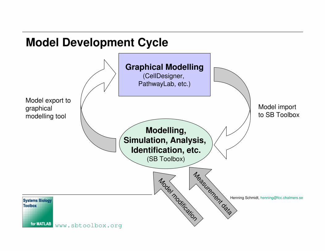
Model Development Cycle
Graphical Modelling(CellDesigner,
PathwayLab, etc.)
Modelling,Simulation, Analysis,
Identification, etc.(SB Toolbox)
Model import to SB Toolbox
Model export to graphical modelling tool
Model modificationMeasurem
ent data
Henning Schmidt, [email protected]
www.sbtoolbox.org
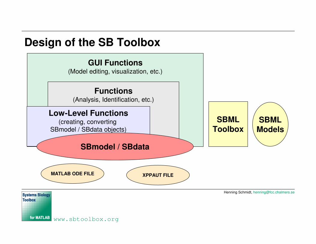
Design of the SB Toolbox
GUI Functions(Model editing, visualization, etc.)
Functions(Analysis, Identification, etc.)
Low-Level Functions(creating, converting
SBmodel / SBdata objects)
SBmodel / SBdata
SBMLToolbox
SBMLModels
XPPAUT FILEMATLAB ODE FILE

Henning Schmidt, [email protected]
www.sbtoolbox.org
SBmodel
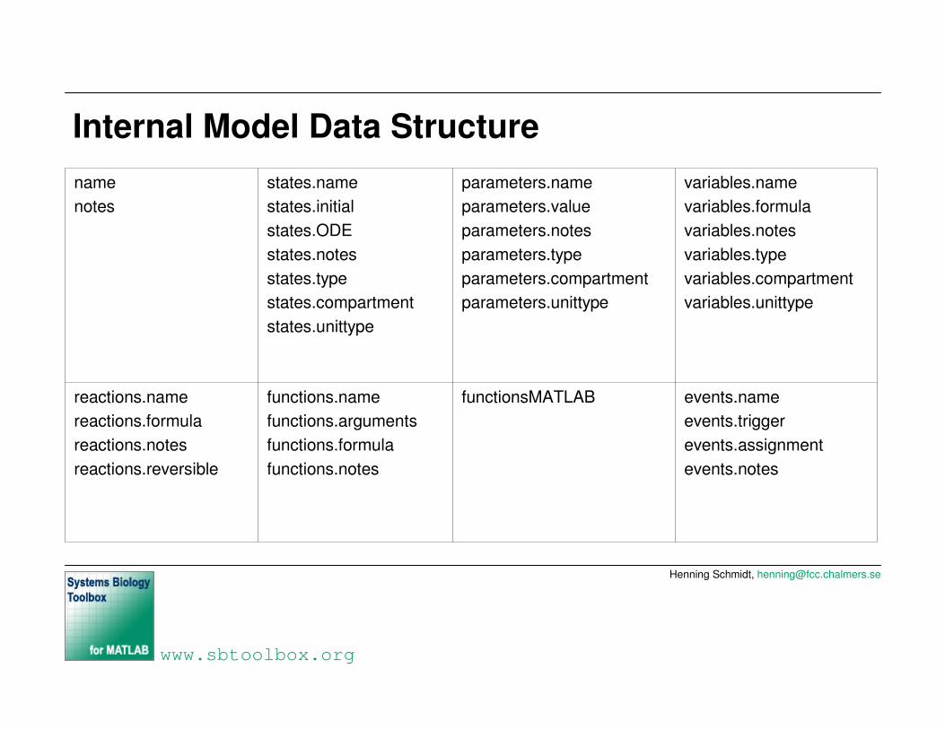
� An SBmodel is realized as an object of class SBmodel� The internal data structure of an SBmodel object is given by
events.nameevents.triggerevents.assignmentevents.notes
functionsMATLABfunctions.namefunctions.argumentsfunctions.formulafunctions.notes
reactions.namereactions.formulareactions.notesreactions.reversible
variables.namevariables.formulavariables.notesvariables.typevariables.compartmentvariables.unittype
parameters.nameparameters.valueparameters.notesparameters.typeparameters.compartmentparameters.unittype
states.name states.initialstates.ODEstates.notesstates.typestates.compartmentstates.unittype
namenotes

Henning Schmidt, [email protected]
www.sbtoolbox.org
SBdata
� A data object is realized as an object of class SBdata� The internal data structure of an SBdata object is given by
measurements.namemeasurements.stimulusflagmeasurements.datameasurements.noiseoffsetmeasurements.noisevariance
timenotesname
Henning Schmidt, [email protected]
www.sbtoolbox.org
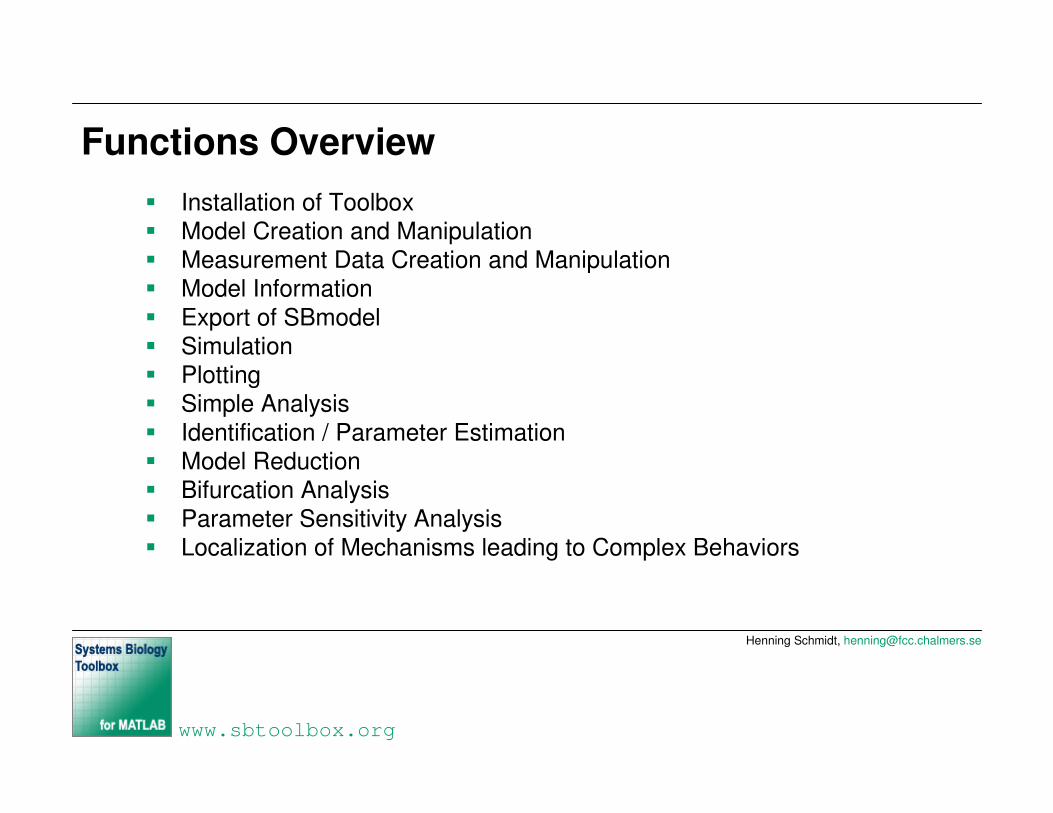
Functions Overview� Installation of Toolbox� Model Creation and Manipulation� Measurement Data Creation and Manipulation� Model Information� Export of SBmodel� Simulation� Plotting� Simple Analysis� Identification / Parameter Estimation� Model Reduction � Bifurcation Analysis� Parameter Sensitivity Analysis � Localization of Mechanisms leading to Complex Behaviors
Henning Schmidt, [email protected]
www.sbtoolbox.org
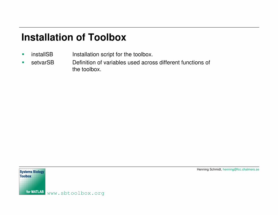
Installation of Toolbox
� installSB Installation script for the toolbox.� setvarSB Definition of variables used across different functions of
the toolbox.

Henning Schmidt, [email protected]
www.sbtoolbox.org
Model Creation and Manipulation
� SBmodel Creating an SBmodel.� SBstruct Returns the internal data structure of an SBmodel as a
MATLAB structure.� SBedit Graphical user interface, allowing to create and/or edit SBmodels in an
ODE based format.� SBeditBC Graphical user interface, allowing to create and/or edit SBmodels in a
reaction equation based format.

Henning Schmidt, [email protected]
www.sbtoolbox.org
Export of SBmodel
� SBcreateODEfile Converting an SBmodel to a MATLAB ODE file.� SBcreateTempODEfile Same as SBcreateODEfile but ODE file is created in the
systems temporary directory.� deleteTempODEfileSB Deletes the ODE file created in the systems temporary
directory.� SBcreateXPPAUTfile Converting an SBmodel to an ODE file that can be used for
simulation and bifurcation analysis by XPPAUT.� SBcreateTEXTfile Converting an SBmodel to an ODE text file description.� SBcreateTEXTBCfile Converting an SBmodel to a biochemically oriented text file
description.� SBexportSBML Exports an SBmodel to an SBML model.� SBconvert2MA SBmodels containing only MA kinetics can have these
extracted and returned in a structure. E.g., for stochastic simulation
Henning Schmidt, [email protected]
www.sbtoolbox.org
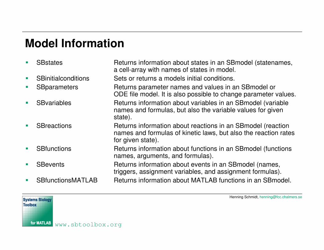
Model Information� SBstates Returns information about states in an SBmodel (statenames,
a cell-array with names of states in model.� SBinitialconditions Sets or returns a models initial conditions.� SBparameters Returns parameter names and values in an SBmodel or
ODE file model. It is also possible to change parameter values.� SBvariables Returns information about variables in an SBmodel (variable
names and formulas, but also the variable values for given state).
� SBreactions Returns information about reactions in an SBmodel (reaction names and formulas of kinetic laws, but also the reaction rates for given state).
� SBfunctions Returns information about functions in an SBmodel (functions names, arguments, and formulas).
� SBevents Returns information about events in an SBmodel (names, triggers, assignment variables, and assignment formulas).
� SBfunctionsMATLAB Returns information about MATLAB functions in an SBmodel.
Henning Schmidt, [email protected]
www.sbtoolbox.org
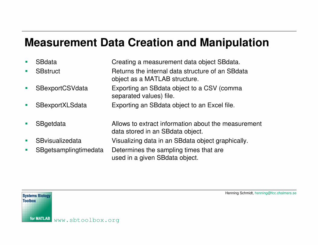
Measurement Data Creation and Manipulation
� SBdata Creating a measurement data object SBdata.� SBstruct Returns the internal data structure of an SBdata
object as a MATLAB structure.� SBexportCSVdata Exporting an SBdata object to a CSV (comma
separated values) file.� SBexportXLSdata Exporting an SBdata object to an Excel file.
� SBgetdata Allows to extract information about the measurement data stored in an SBdata object.
� SBvisualizedata Visualizing data in an SBdata object graphically.� SBgetsamplingtimedata Determines the sampling times that are
used in a given SBdata object.
Henning Schmidt, [email protected]
www.sbtoolbox.org
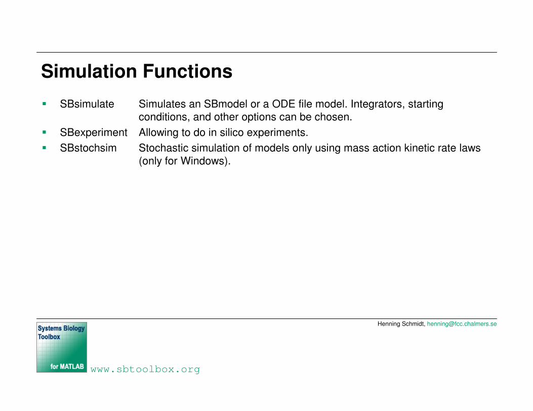
Simulation Functions
� SBsimulate Simulates an SBmodel or a ODE file model. Integrators, starting conditions, and other options can be chosen.
� SBexperiment Allowing to do in silico experiments.� SBstochsim Stochastic simulation of models only using mass action kinetic rate laws
(only for Windows).
Henning Schmidt, [email protected]
www.sbtoolbox.org
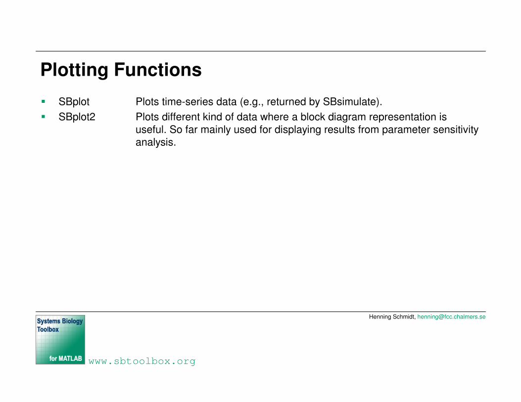
Plotting Functions
� SBplot Plots time-series data (e.g., returned by SBsimulate).� SBplot2 Plots different kind of data where a block diagram representation is
useful. So far mainly used for displaying results from parameter sensitivity analysis.
Henning Schmidt, [email protected]
www.sbtoolbox.org
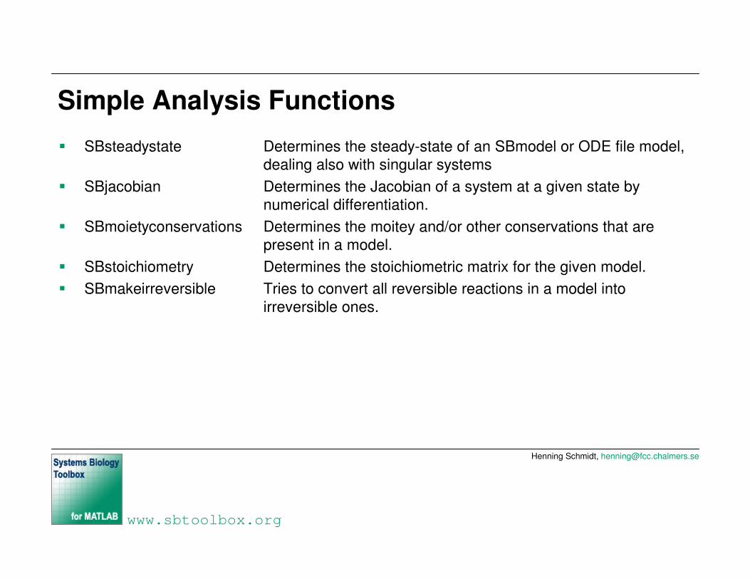
Simple Analysis Functions
� SBsteadystate Determines the steady-state of an SBmodel or ODE file model, dealing also with singular systems
� SBjacobian Determines the Jacobian of a system at a given state by numerical differentiation.
� SBmoietyconservations Determines the moitey and/or other conservations that are present in a model.
� SBstoichiometry Determines the stoichiometric matrix for the given model.� SBmakeirreversible Tries to convert all reversible reactions in a model into
irreversible ones.
Henning Schmidt, [email protected]
www.sbtoolbox.org
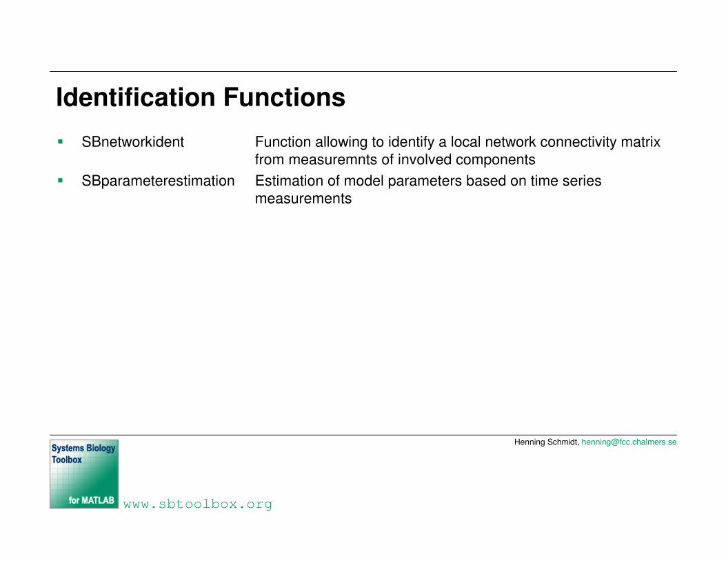
Identification Functions
� SBnetworkident Function allowing to identify a local network connectivity matrix from measuremnts of involved components
� SBparameterestimation Estimation of model parameters based on time series measurements

Henning Schmidt, [email protected]
www.sbtoolbox.org
Model Reduction Functions
� SBreducemodel Allows to reduce a singular model to a non-singular by deleting algebraic relations from the ODEs, and replacing them by variables.

Henning Schmidt, [email protected]
www.sbtoolbox.org
Bifurcation Analysis Functions
� SBxppaut Starts XPPAUT with the given XPPAUT ODE file.� SBplotxppaut Plot bifurcation data file saved from AUTO/XPPAUT.
Henning Schmidt, [email protected]
www.sbtoolbox.org
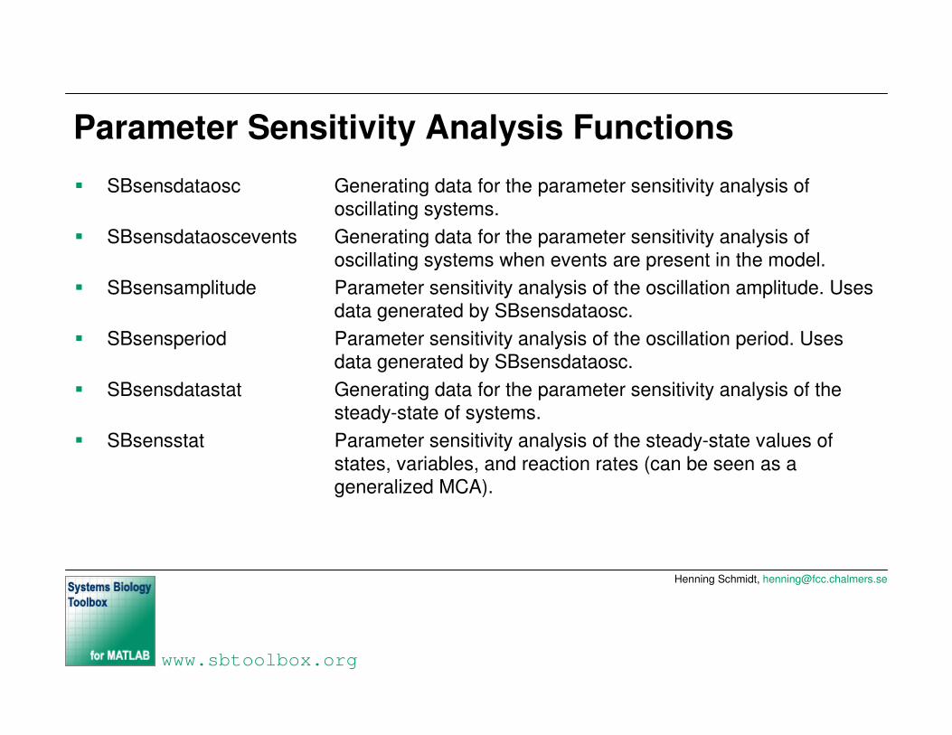
Parameter Sensitivity Analysis Functions
� SBsensdataosc Generating data for the parameter sensitivity analysis of oscillating systems.
� SBsensdataoscevents Generating data for the parameter sensitivity analysis of oscillating systems when events are present in the model.
� SBsensamplitude Parameter sensitivity analysis of the oscillation amplitude. Uses data generated by SBsensdataosc.
� SBsensperiod Parameter sensitivity analysis of the oscillation period. Uses data generated by SBsensdataosc.
� SBsensdatastat Generating data for the parameter sensitivity analysis of the steady-state of systems.
� SBsensstat Parameter sensitivity analysis of the steady-state values of states, variables, and reaction rates (can be seen as a generalized MCA).
Henning Schmidt, [email protected]
www.sbtoolbox.org
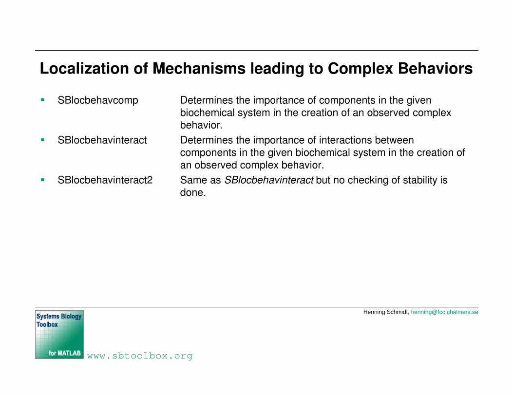
Localization of Mechanisms leading to Complex Behaviors
� SBlocbehavcomp Determines the importance of components in the given biochemical system in the creation of an observed complex behavior.
� SBlocbehavinteract Determines the importance of interactions between components in the given biochemical system in the creation of an observed complex behavior.
� SBlocbehavinteract2 Same as SBlocbehavinteract but no checking of stability is done.

Henning Schmidt, [email protected]
www.sbtoolbox.org
Using the toolbox documentation
� Documentation can be found on the webpage www.sbtoolbox.org� Download and installation guide� User’s reference manual (including examples for all functions)
� MATLAB documentation
>> help SBTOOLBOX
>> help ”functionname”
>> help SBmodel
Henning Schmidt, [email protected]
www.sbtoolbox.org
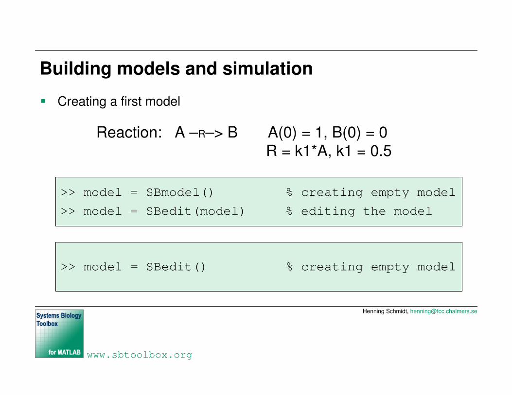
Building models and simulation
� Creating a first model
>> model = SBmodel() % creating empty model
>> model = SBedit(model) % editing the model
Reaction: A –R–> B A(0) = 1, B(0) = 0R = k1*A, k1 = 0.5
>> model = SBedit() % creating empty model
Henning Schmidt, [email protected]
www.sbtoolbox.org
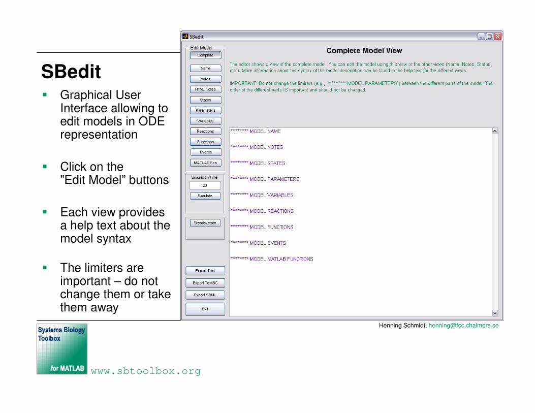
SBedit� Graphical User
Interface allowing to edit models in ODE representation
� Click on the ”Edit Model” buttons
� Each view providesa help text about themodel syntax
� The limiters are important – do not change them or take them away

Henning Schmidt, [email protected]
www.sbtoolbox.org
Simple model (States, Parameters, Reactions)
� Enter the following information (keep all non used limiters)
********** MODEL NAMESimple model********** MODEL STATESd/dt(A) = -Rd/dt(B) = RA(0) = 1B(0) = 0********** MODEL PARAMETERSk1 = 0.5********** MODEL REACTIONSR = k1*A
A –R–> B
A(0) = 1B(0) = 0
k1 = 0.5
R = k1*A
Henning Schmidt, [email protected]
www.sbtoolbox.org
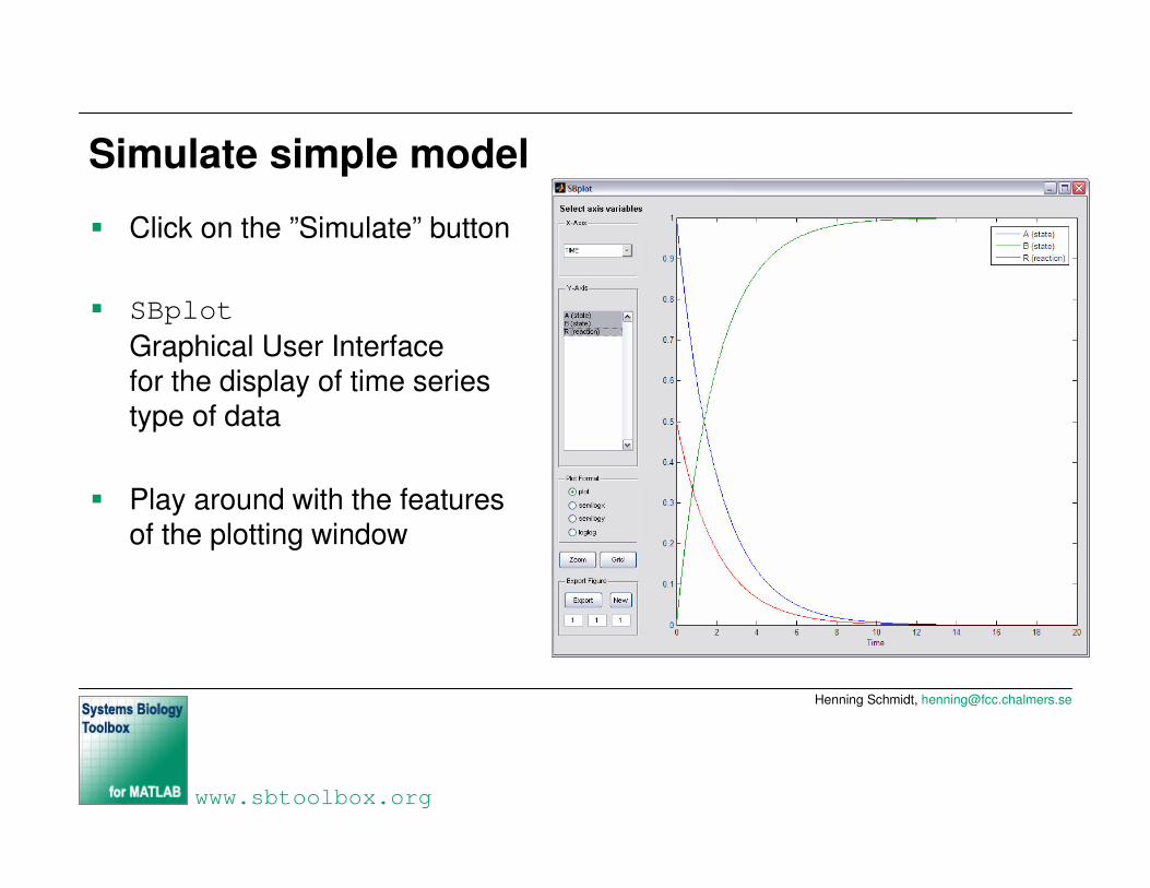
Simulate simple model
� Click on the ”Simulate” button
� SBplotGraphical User Interfacefor the display of time seriestype of data
� Play around with the features of the plotting window

Henning Schmidt, [email protected]
www.sbtoolbox.org
Model Functions
� Model functions can be used to define often recurring calculations
********** MODEL STATESd/dt(A) = -Rd/dt(B) = RA(0) = 1B(0) = 0********** MODEL PARAMETERSk1 = 0.5********** MODEL REACTIONSR = k1*f(A)********** MODEL FUNCTIONSf(x) = x^3
A –R–> B
A(0) = 1B(0) = 0
k1 = 0.5
R = k1*f(A)
f(x) = x^3
Click ”Simulate”
Henning Schmidt, [email protected]
www.sbtoolbox.org
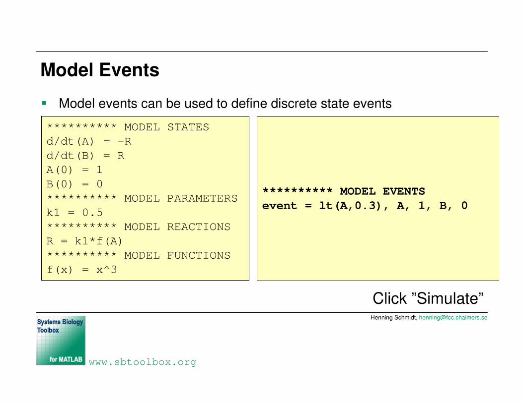
Model Events
� Model events can be used to define discrete state events
********** MODEL STATESd/dt(A) = -Rd/dt(B) = RA(0) = 1B(0) = 0********** MODEL PARAMETERSk1 = 0.5********** MODEL REACTIONSR = k1*f(A)********** MODEL FUNCTIONSf(x) = x^3
********** MODEL EVENTSevent = lt(A,0.3), A, 1, B, 0
Click ”Simulate”
Henning Schmidt, [email protected]
www.sbtoolbox.org
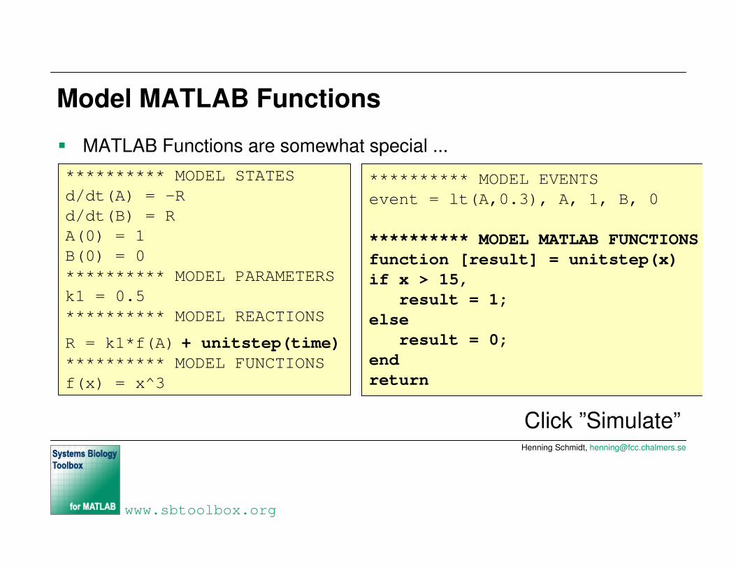
Model MATLAB Functions
� MATLAB Functions are somewhat special ...********** MODEL STATESd/dt(A) = -Rd/dt(B) = RA(0) = 1B(0) = 0********** MODEL PARAMETERSk1 = 0.5********** MODEL REACTIONS
R = k1*f(A) + unitstep(time)********** MODEL FUNCTIONSf(x) = x^3
********** MODEL EVENTSevent = lt(A,0.3), A, 1, B, 0
********** MODEL MATLAB FUNCTIONSfunction [result] = unitstep(x)if x > 15,
result = 1;else
result = 0;endreturn
Click ”Simulate”

Henning Schmidt, [email protected]
www.sbtoolbox.org
Model Variables
� Simulation of these two models gives exactly the same results
********** MODEL NAMESimple model********** MODEL STATESd/dt(A) = -Rd/dt(B) = RA(0) = 1B(0) = 0********** MODEL PARAMETERSk1 = 0.5********** MODEL REACTIONSR = k1*A
********** MODEL NAMESimple model********** MODEL STATESd/dt(A) = -Rd/dt(B) = RA(0) = 1B(0) = 0********** MODEL PARAMETERSk1 = 0.5********** MODEL VARIABLESR = k1*A
So what is the difference?
Henning Schmidt, [email protected]
www.sbtoolbox.org
Model Reactions vs. Model Variables
� Reaction definitions should be reaction rates� Variable definitions should be used for intermediate calculations
� The only cases where it matters for the toolbox is when� Determining the stoichiometric matrix� Exporting the model to SBML
We will see both cases later

Henning Schmidt, [email protected]
www.sbtoolbox.org
Command Line Simulation
� Click ”Exit” in the SBedit GUI to return the model to the workspace
>> model = SBedit()SBmodel=======Name: Simple ModelNumber States: 2Number Variables: 0Number Parameters: 1Number Reactions: 1Number Functions: 1Number Events: 1MATLAB functions present
>> SBsimulate(model,50) % simulation over 50 time units

Henning Schmidt, [email protected]
www.sbtoolbox.org
Simulation, continued
>> output = SBsimulate(model,50)output =
time: [50x1 double]states: {'A' 'B'}
statevalues: [50x2 double]variables: {}
variablevalues: []reactions: {'R'}
reactionvalues: [50x1 double]
>> help SBsimulate
>> output = SBsimulate(model,’ode45’,[0:0.1:100],[2 0])
Integrator
Time vector
Initial conditions
Henning Schmidt, [email protected]
www.sbtoolbox.org
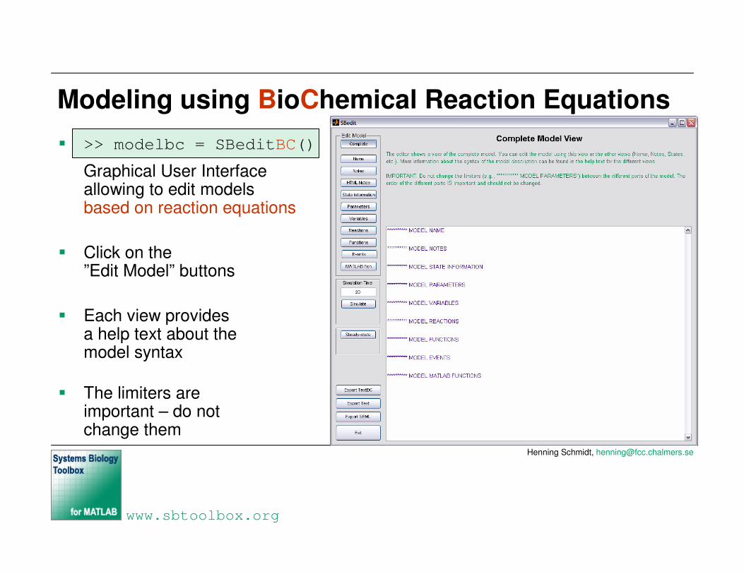
Modeling using BioChemical Reaction Equations� >> modelbc = SBeditBC()
Graphical User Interface allowing to edit models based on reaction equations
� Click on the ”Edit Model” buttons
� Each view providesa help text about themodel syntax
� The limiters are important – do not change them
Henning Schmidt, [email protected]
www.sbtoolbox.org
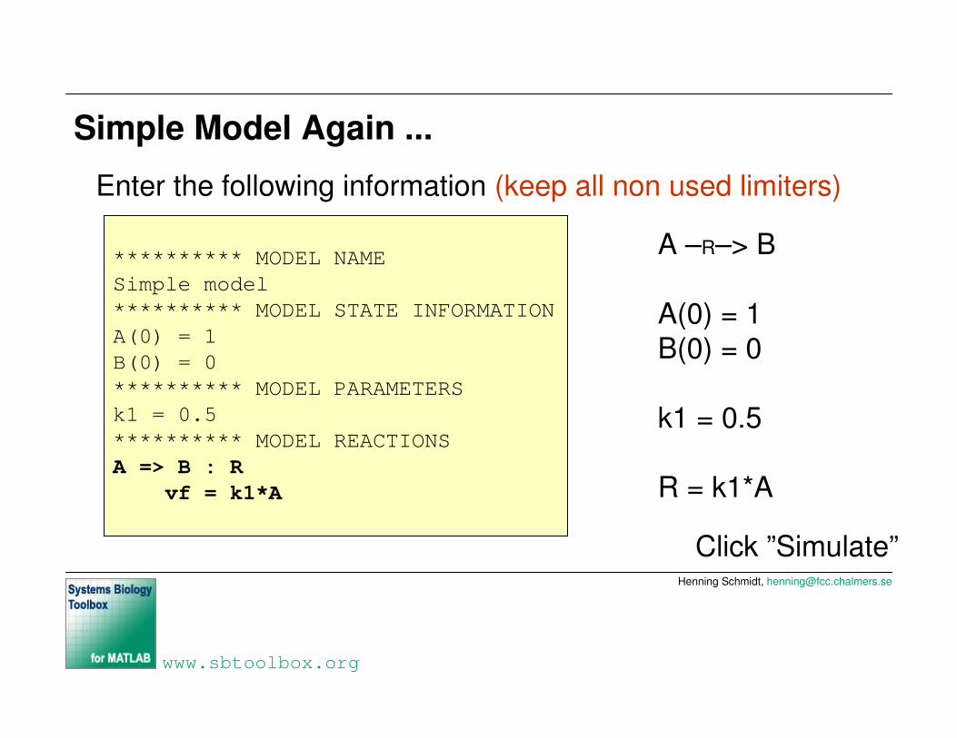
Simple Model Again ...
********** MODEL NAMESimple model********** MODEL STATE INFORMATIONA(0) = 1B(0) = 0********** MODEL PARAMETERSk1 = 0.5********** MODEL REACTIONSA => B : R
vf = k1*A
A –R–> B
A(0) = 1B(0) = 0
k1 = 0.5
R = k1*A
Click ”Simulate”
Enter the following information (keep all non used limiters)
Henning Schmidt, [email protected]
www.sbtoolbox.org
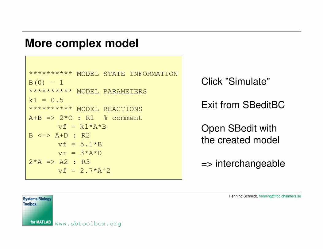
More complex model
********** MODEL STATE INFORMATIONB(0) = 1********** MODEL PARAMETERSk1 = 0.5********** MODEL REACTIONSA+B => 2*C : R1 % comment
vf = k1*A*BB <=> A+D : R2
vf = 5.1*Bvr = 3*A*D
2*A => A2 : R3vf = 2.7*A^2
Click ”Simulate”
Exit from SBeditBC
Open SBedit with the created model
=> interchangeable
Henning Schmidt, [email protected]
www.sbtoolbox.org
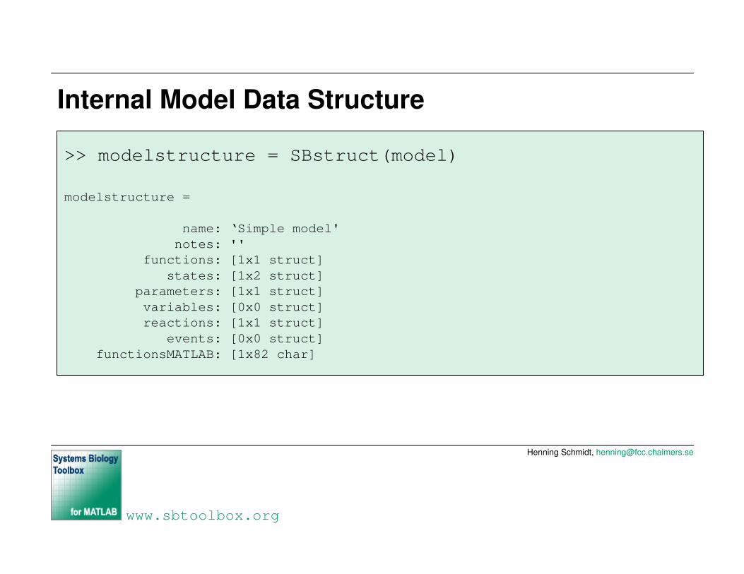
Internal Model Data Structure
>> modelstructure = SBstruct(model)
modelstructure =
name: ‘Simple model'notes: ''
functions: [1x1 struct]states: [1x2 struct]
parameters: [1x1 struct]variables: [0x0 struct]reactions: [1x1 struct]
events: [0x0 struct]functionsMATLAB: [1x82 char]
Henning Schmidt, [email protected]
www.sbtoolbox.org
Internal Model Data Structure
events.nameevents.triggerevents.assignmentevents.notes
functionsMATLABfunctions.namefunctions.argumentsfunctions.formulafunctions.notes
reactions.namereactions.formulareactions.notesreactions.reversible
variables.namevariables.formulavariables.notesvariables.typevariables.compartmentvariables.unittype
parameters.nameparameters.valueparameters.notesparameters.typeparameters.compartmentparameters.unittype
states.name states.initialstates.ODEstates.notesstates.typestates.compartmentstates.unittype
namenotes

Henning Schmidt, [email protected]
www.sbtoolbox.org
Editing the Structure and Converting to SBmodel
>> modelstructure.parameters(1)ans =
name: 'k1'value: 0.5000notes: ''
sbmlnotes: ''
>> modelstructure.parameters(1).value = 2>> modelstructure.parameters(2).name = ’k2’;>> modelstructure.parameters(2).value = 1;
>> modelchanged = SBmodel(modelstructure)
>> SBedit(modelchanged)
Changing parameter value
Adding new parameter


Henning Schmidt, [email protected]
www.sbtoolbox.org
Export a Model to the Textual Description
� To export a model to the ODE / Biochemical textual description using SBedit or SBeditBC click ”Export Text” / ”Export TextBC”
� Choose a file name – here: textmodel.txt / textmodel.txtbc
� ODE textmodel files are required to have the extension .txt� Biochemical textmodel files are required to have the extension .txtbc
� Click ”Exit”
>> SBedit(modelchanged)

Henning Schmidt, [email protected]
www.sbtoolbox.org
Import a Textual Description to an SBmodel
� Open the textmodel file with the MATLAB editor to see its syntax
� To import the text(BC) model and convert it to an SBmodel write
>> edit textmodel.txtor>> edit textmodel.txtbc
>> model = SBmodel(‘textmodel.txt’)or>> model = SBmodel(‘textmodel.txtbc’)

Henning Schmidt, [email protected]
www.sbtoolbox.org
Import of SBML Models
� SBML Level 1 and 2 models can be imported� Change into the tutorials example files folder
>> model = SBmodel(’CellCycle.xml’)
SBmodel=======Name: CellCycleNumber States: 13Number Variables: 2Number Parameters: 41Number Reactions: 23Number Functions: 1
>> SBedit(model)
Increase simulation time to 400 and click ”Simulate”

Henning Schmidt, [email protected]
www.sbtoolbox.org
Export of SBML Models
� Export only to SBML Level 2
� The SBML Toolbox needs to be present
� The export functionality is disabled in version 1.5. We are currently working on an improved SBML export function

Henning Schmidt, [email protected]
www.sbtoolbox.org
Moiety conservations
� Determination of moiety conservations
� In case of ”bad” results the tolerance might need to be adjusted
>> model = SBmodel(’CellCycle.xml’)>> model = SBmodel(’CellCycle.txt’) (if no SBML Toolbox)>> SBmoietyconservations(model)
Cdc25P = 1 - 1 Cdc25Wee1 = 1 - 1 Wee1PAPC_ = 1 - 1 APCIEP = 1 - 1 IE
>> help SBmoietyconservations
Henning Schmidt, [email protected]
www.sbtoolbox.org
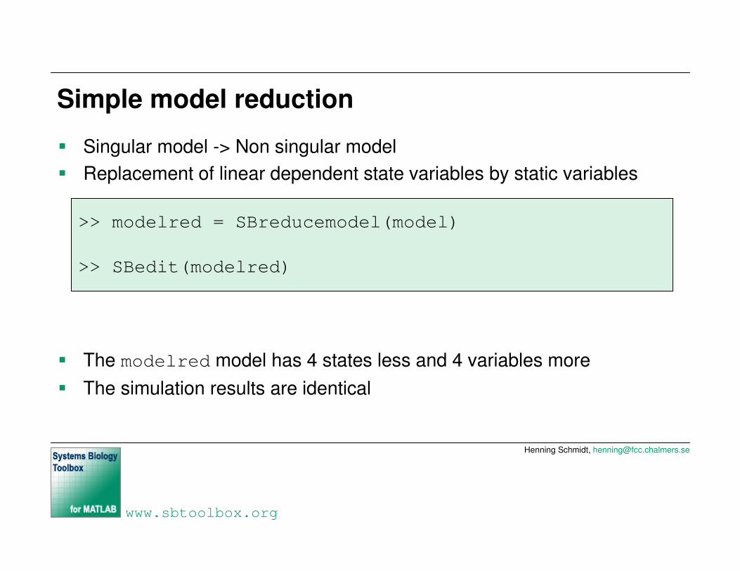
Simple model reduction
� Singular model -> Non singular model � Replacement of linear dependent state variables by static variables
� The modelred model has 4 states less and 4 variables more� The simulation results are identical
>> modelred = SBreducemodel(model)
>> SBedit(modelred)
Henning Schmidt, [email protected]
www.sbtoolbox.org
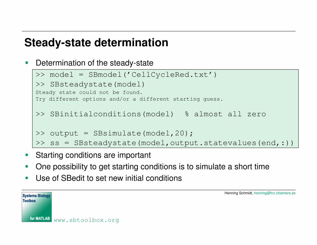
Steady-state determination
� Determination of the steady-state
� Starting conditions are important� One possibility to get starting conditions is to simulate a short time� Use of SBedit to set new initial conditions
>> model = SBmodel(’CellCycleRed.txt’)>> SBsteadystate(model)Steady state could not be found. Try different options and/or a different starting guess.
>> SBinitialconditions(model) % almost all zero
>> output = SBsimulate(model,20);>> ss = SBsteadystate(model,output.statevalues(end,:))

Henning Schmidt, [email protected]
www.sbtoolbox.org
Jacobian and stability
� Determination of the Jacobian
� Determination of stability by considering the Jacobian eigenvalues
� Two complex conjugated eigenvalues with positive real part=> the considered steady-state is unstable and the system is oscillating
around it
>> Jacobian = SBjacobian(model,ss)
>> eig(Jacobian)
0.0413 + 0.1528i0.0413 - 0.1528i...

Henning Schmidt, [email protected]
www.sbtoolbox.org
Bifurcation analysis
� Bifurcation analysis is realized using the XPPAUT software� The toolbox provides an interface to XPPAUT
� Alternatively
� Under Windows an X-Server needs to be present� XPPAUT limitations (10 characters, case insensitive)
>> model = SBmodel(’CellCycle2.txt’)>> SBcreateXPPAUTfile(model)
>> model = SBmodel(’CellCycle2.txt’)>> SBxppaut(model,ss)
Henning Schmidt, [email protected]
www.sbtoolbox.org
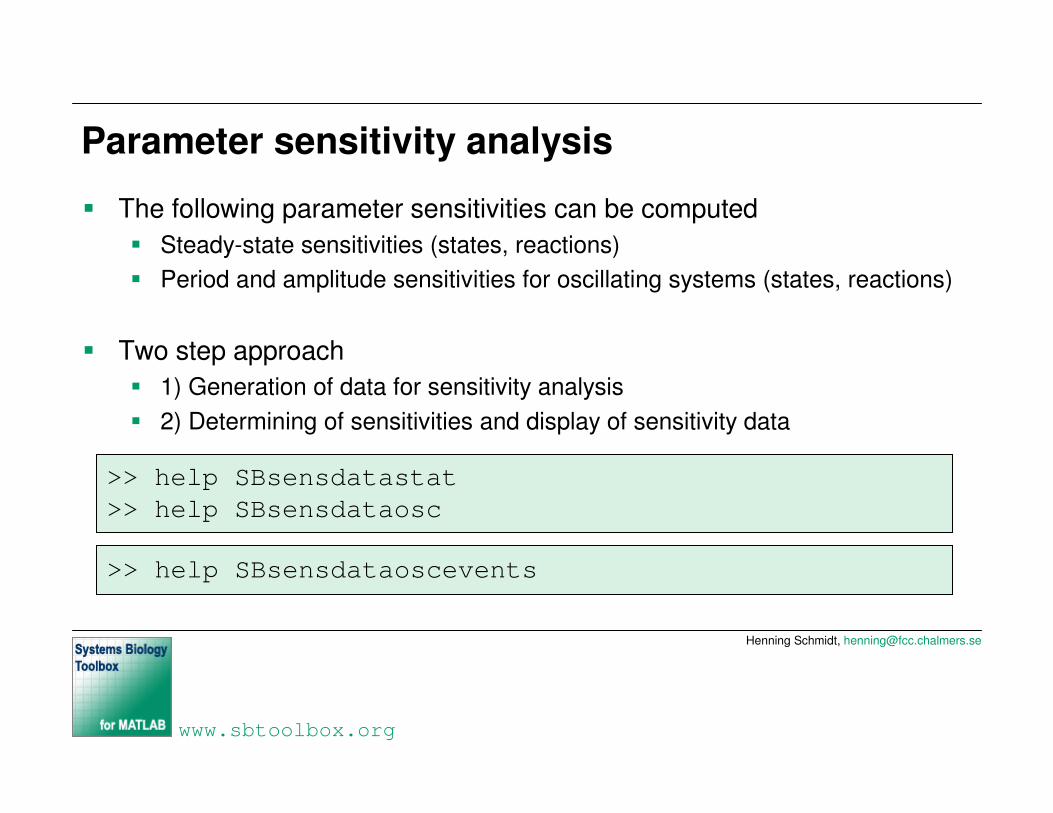
Parameter sensitivity analysis
� The following parameter sensitivities can be computed� Steady-state sensitivities (states, reactions)� Period and amplitude sensitivities for oscillating systems (states, reactions)
� Two step approach� 1) Generation of data for sensitivity analysis� 2) Determining of sensitivities and display of sensitivity data
>> help SBsensdatastat>> help SBsensdataosc
>> help SBsensdataoscevents
Henning Schmidt, [email protected]
www.sbtoolbox.org
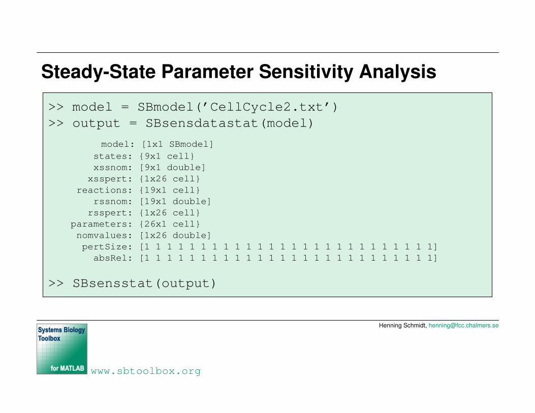
Steady-State Parameter Sensitivity Analysis
>> model = SBmodel(’CellCycle2.txt’)>> output = SBsensdatastat(model)
model: [1x1 SBmodel]states: {9x1 cell}xssnom: [9x1 double]xsspert: {1x26 cell}
reactions: {19x1 cell}rssnom: [19x1 double]rsspert: {1x26 cell}
parameters: {26x1 cell}nomvalues: [1x26 double]pertSize: [1 1 1 1 1 1 1 1 1 1 1 1 1 1 1 1 1 1 1 1 1 1 1 1 1 1]absRel: [1 1 1 1 1 1 1 1 1 1 1 1 1 1 1 1 1 1 1 1 1 1 1 1 1 1]
>> SBsensstat(output)
Henning Schmidt, [email protected]
www.sbtoolbox.org
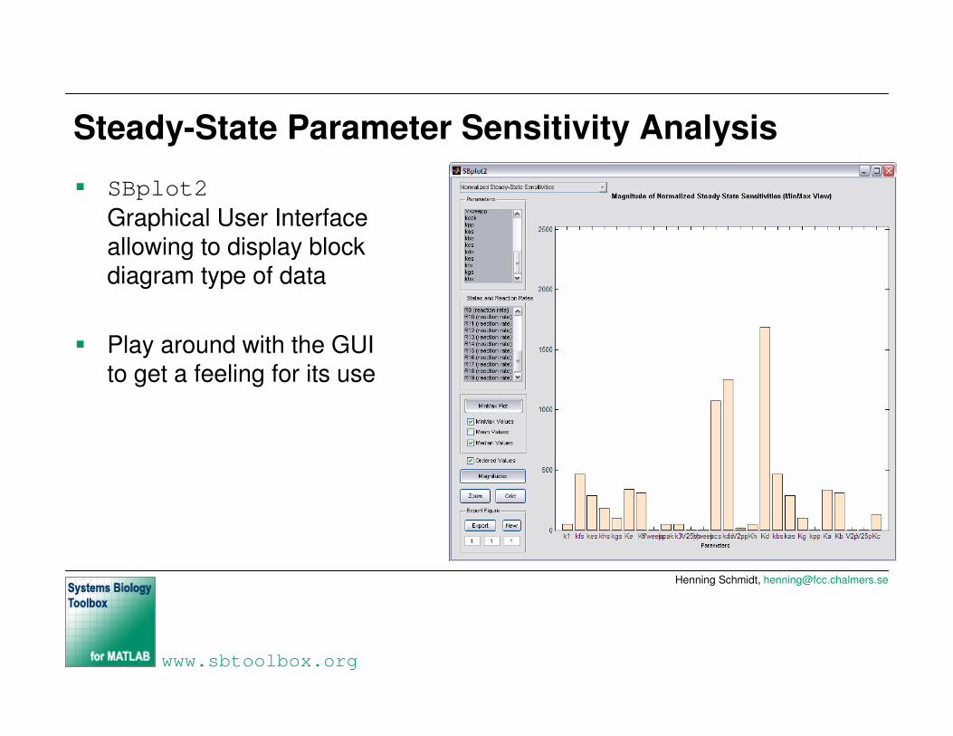
Steady-State Parameter Sensitivity Analysis
� SBplot2Graphical User Interfaceallowing to display blockdiagram type of data
� Play around with the GUIto get a feeling for its use
Henning Schmidt, [email protected]
www.sbtoolbox.org
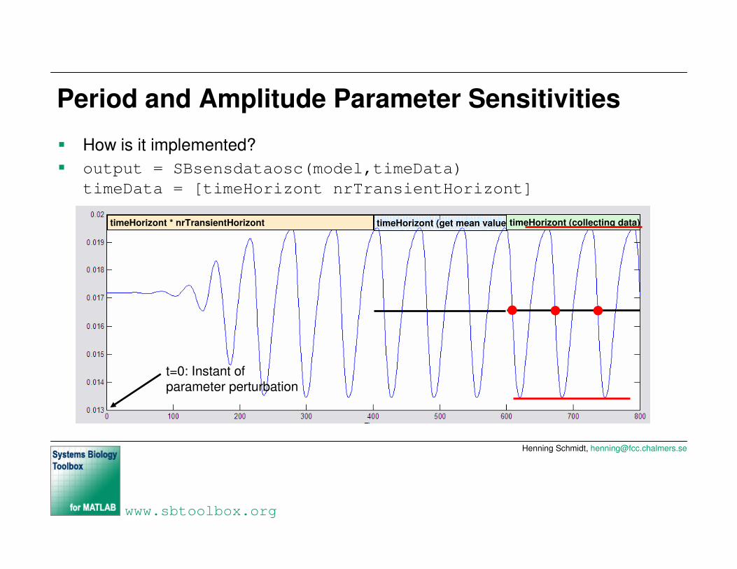
Period and Amplitude Parameter Sensitivities
� How is it implemented?� output = SBsensdataosc(model,timeData)
timeData = [timeHorizont nrTransientHorizont]
timeHorizont * nrTransientHorizont timeHorizont (get mean values)timeHorizont (collecting data)
• • •
t=0: Instant of parameter perturbation
Henning Schmidt, [email protected]
www.sbtoolbox.org
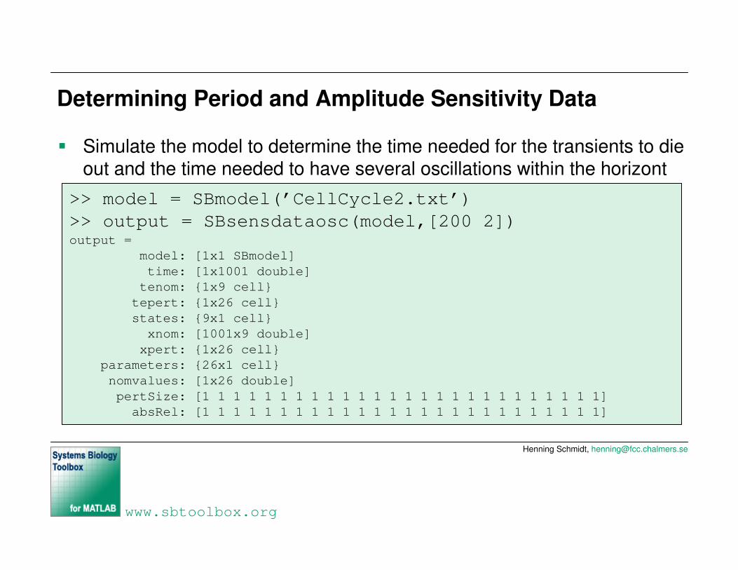
Determining Period and Amplitude Sensitivity Data
� Simulate the model to determine the time needed for the transients to die out and the time needed to have several oscillations within the horizont
>> model = SBmodel(’CellCycle2.txt’)>> output = SBsensdataosc(model,[200 2])output =
model: [1x1 SBmodel]time: [1x1001 double]tenom: {1x9 cell}tepert: {1x26 cell}states: {9x1 cell}xnom: [1001x9 double]xpert: {1x26 cell}
parameters: {26x1 cell}nomvalues: [1x26 double]pertSize: [1 1 1 1 1 1 1 1 1 1 1 1 1 1 1 1 1 1 1 1 1 1 1 1 1 1]absRel: [1 1 1 1 1 1 1 1 1 1 1 1 1 1 1 1 1 1 1 1 1 1 1 1 1 1]
Henning Schmidt, [email protected]
www.sbtoolbox.org
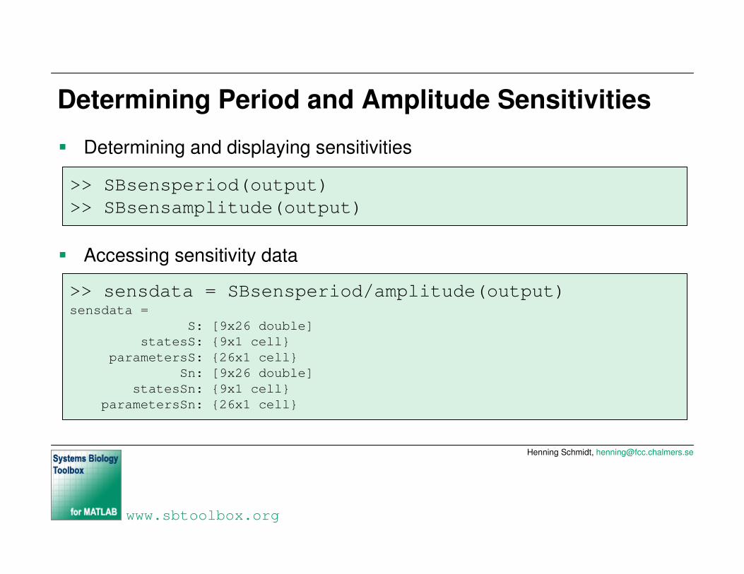
Determining Period and Amplitude Sensitivities
� Determining and displaying sensitivities
� Accessing sensitivity data
>> SBsensperiod(output)>> SBsensamplitude(output)
>> sensdata = SBsensperiod/amplitude(output)sensdata =
S: [9x26 double]statesS: {9x1 cell}
parametersS: {26x1 cell}Sn: [9x26 double]
statesSn: {9x1 cell}parametersSn: {26x1 cell}
Henning Schmidt, [email protected]
www.sbtoolbox.org
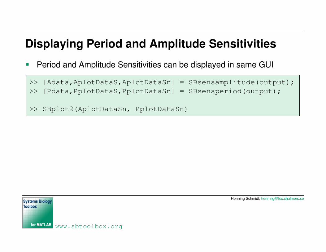
Displaying Period and Amplitude Sensitivities
� Period and Amplitude Sensitivities can be displayed in same GUI
>> [Adata,AplotDataS,AplotDataSn] = SBsensamplitude(output);>> [Pdata,PplotDataS,PplotDataSn] = SBsensperiod(output);
>> SBplot2(AplotDataSn, PplotDataSn)

Henning Schmidt, [email protected]
www.sbtoolbox.org
In silico experiments and the representation of measurement data� In silico experiments are a different way of simulating a model� You can specify
� Measured components (states, variables, and/or reaction rates)� Perturbations on parameters during the experiment� Noise to be added to the measurements
� The experiment starts always at the initial state that is specified in the model. If you want to start at a specific state you will have to set this state correctly in the model by using SBedit or the SBinitialconditions function
>> help SBexperiment

Henning Schmidt, [email protected]
www.sbtoolbox.org
Performing an in silico experiment
� Define the model to use
� We want to start the experiment in the steady-state
� Define the measurements� We want to measure all states with a sampling time of 0.01h until 0.2h
>> model = SBmodel(’kholodenko4gene.txt’)
>> ss = SBsteadystate(model)>> model = SBinitialconditions(model, ss)
>> deltaT = 0.01>> maxTime = 0.2>> measurements = {’states’,[deltaT,maxTime]}
Henning Schmidt, [email protected]
www.sbtoolbox.org
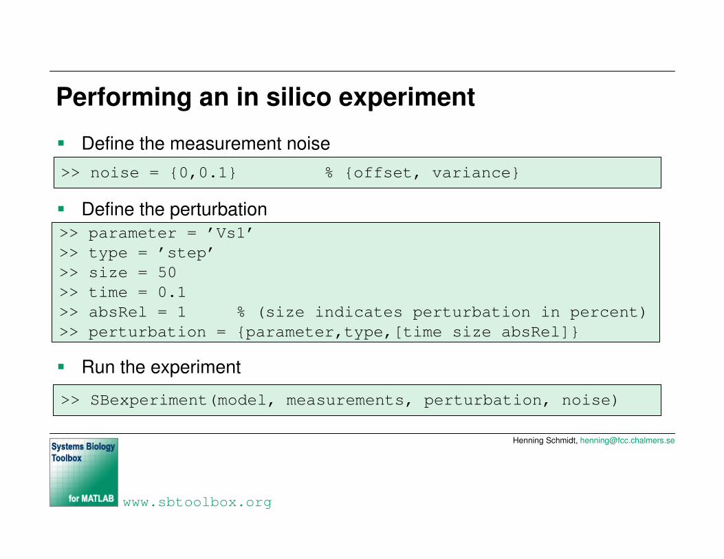
Performing an in silico experiment
� Define the measurement noise
� Define the perturbation
� Run the experiment
>> noise = {0,0.1} % {offset, variance}
>> parameter = ’Vs1’>> type = ’step’>> size = 50>> time = 0.1>> absRel = 1 % (size indicates perturbation in percent)>> perturbation = {parameter,type,[time size absRel]}
>> SBexperiment(model, measurements, perturbation, noise)
Henning Schmidt, [email protected]
www.sbtoolbox.org
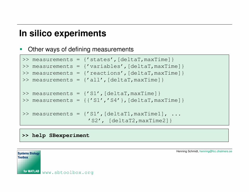
In silico experiments
� Other ways of defining measurements>> measurements = {’states’,[deltaT,maxTime]}>> measurements = {’variables’,[deltaT,maxTime]}>> measurements = {’reactions’,[deltaT,maxTime]}>> measurements = {’all’,[deltaT,maxTime]}
>> measurements = {’S1’,[deltaT,maxTime]}>> measurements = {{’S1’,’S4’},[deltaT,maxTime]}
>> measurements = {’S1’,[deltaT1,maxTime1], ...’S2’, [deltaT2,maxTime2]}
>> help SBexperiment
Henning Schmidt, [email protected]
www.sbtoolbox.org
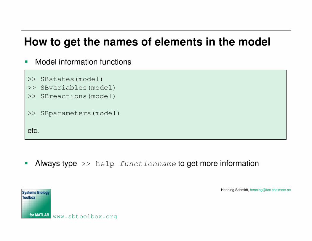
How to get the names of elements in the model
� Model information functions
� Always type >> help functionname to get more information
>> SBstates(model)>> SBvariables(model)>> SBreactions(model)
>> SBparameters(model)
etc.
Henning Schmidt, [email protected]
www.sbtoolbox.org
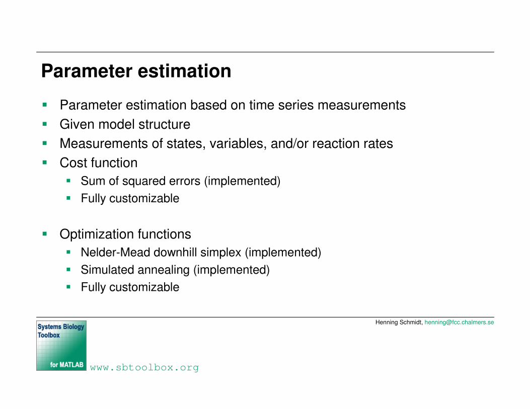
Parameter estimation
� Parameter estimation based on time series measurements � Given model structure� Measurements of states, variables, and/or reaction rates� Cost function
� Sum of squared errors (implemented)� Fully customizable
� Optimization functions� Nelder-Mead downhill simplex (implemented)� Simulated annealing (implemented)� Fully customizable
Henning Schmidt, [email protected]
www.sbtoolbox.org
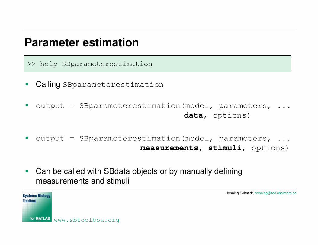
Parameter estimation
� Calling SBparameterestimation
� output = SBparameterestimation(model, parameters, ...data, options)
� output = SBparameterestimation(model, parameters, ...measurements, stimuli, options)
� Can be called with SBdata objects or by manually defining measurements and stimuli
>> help SBparameterestimation

Henning Schmidt, [email protected]
www.sbtoolbox.org
Parameter estimation example
� Define the model
� Import the measurement data
� Have a look at the data files and at the data
>> model = SBmodel(’model.txt’)
>> data = SBdata(’measurements.xls’)alternatively
>> data = SBdata(’measurements.csv’)
>> SBvisualizedata(data)

Henning Schmidt, [email protected]
www.sbtoolbox.org
Parameter estimation example
� Define the parameters to estimate, initial values, and signs
� Define the options for the estimation function
� Run the estimation
>> parameters = []>> parameters.names = {'Ka','Kb','Kc'}>> parameters.initialValues = [10 100 20]>> parameters.signs = [1 1 1]
>> options = []
>> options.optimizer = 'simannealingSB'
>> result = SBparameterestimation(model, parameters, ...data, options)
Henning Schmidt, [email protected]
www.sbtoolbox.org
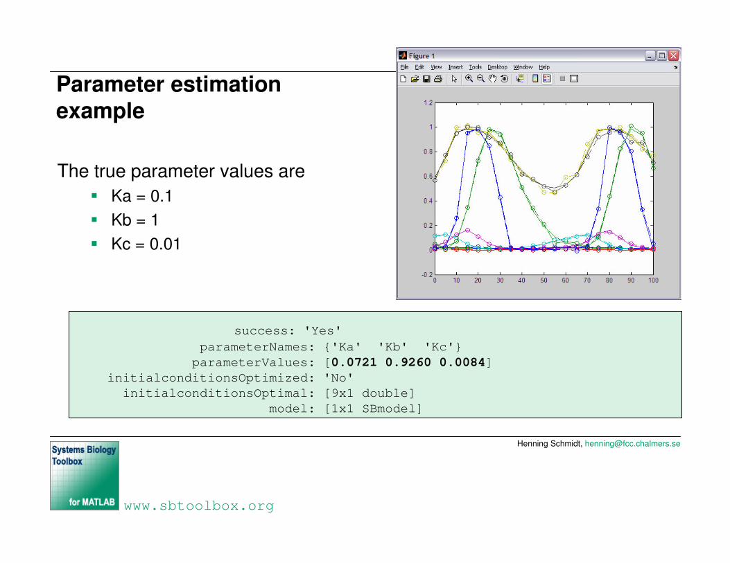
Parameter estimation example
The true parameter values are� Ka = 0.1� Kb = 1� Kc = 0.01
success: 'Yes'parameterNames: {'Ka' 'Kb' 'Kc'}parameterValues: [0.0721 0.9260 0.0084]
initialconditionsOptimized: 'No'initialconditionsOptimal: [9x1 double]
model: [1x1 SBmodel]
Henning Schmidt, [email protected]
www.sbtoolbox.org
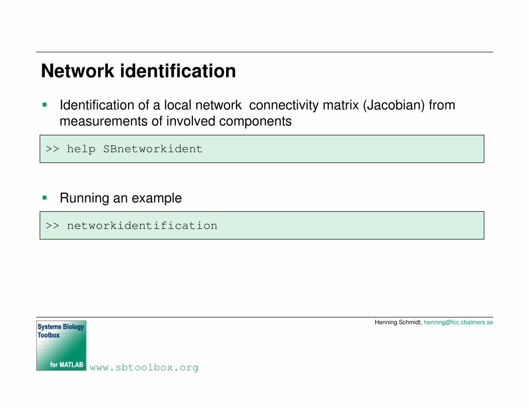
Network identification
� Identification of a local network connectivity matrix (Jacobian) from measurements of involved components
� Running an example
>> help SBnetworkident
>> networkidentification
Henning Schmidt, [email protected]
www.sbtoolbox.org
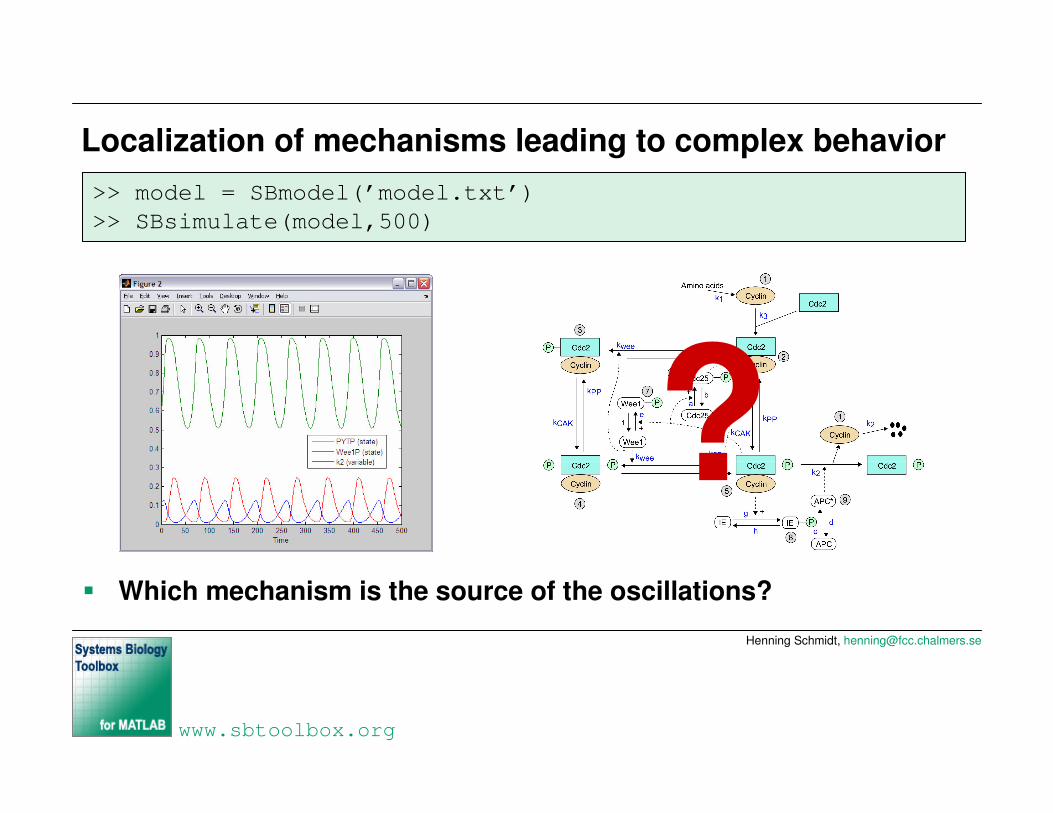
Localization of mechanisms leading to complex behavior
� Which mechanism is the source of the oscillations?
?>> model = SBmodel(’model.txt’)>> SBsimulate(model,500)
Henning Schmidt, [email protected]
www.sbtoolbox.org
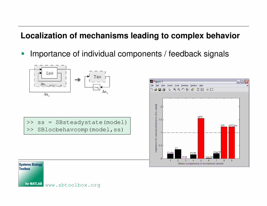
Localization of mechanisms leading to complex behavior
� Importance of individual components / feedback signals
>> ss = SBsteadystate(model)>> SBlocbehavcomp(model,ss)

Henning Schmidt, [email protected]
www.sbtoolbox.org
Localization of mechanisms leading to complex behavior
� Importance of pairwise component interactions
L(s) Lp(s)
>> ss = SBsteadystate(model)>> SBlocbehavinteract(model,ss)

Henning Schmidt, [email protected]
www.sbtoolbox.org
Identified mechanism behind oscillations
� Feedback mechanism involving� 5: YTP� 8: IEP� 9: APC*
Henning Schmidt, [email protected]
www.sbtoolbox.org
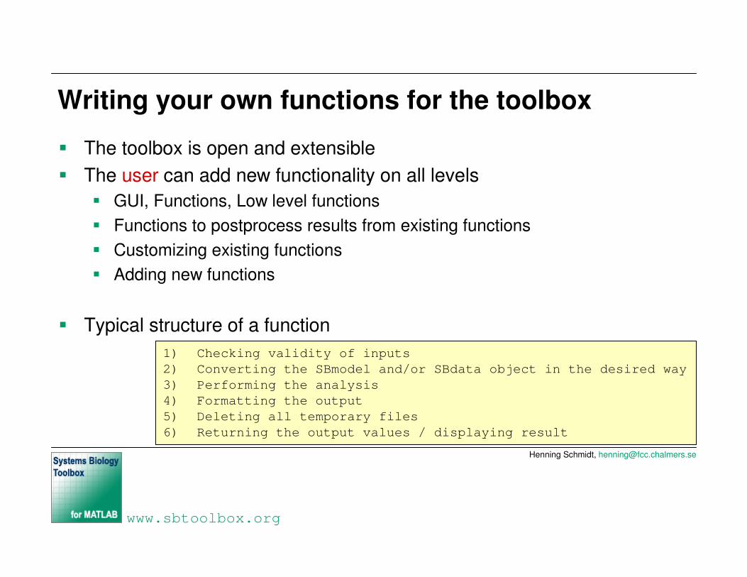
Writing your own functions for the toolbox
� The toolbox is open and extensible� The user can add new functionality on all levels
� GUI, Functions, Low level functions� Functions to postprocess results from existing functions� Customizing existing functions� Adding new functions
� Typical structure of a function1) Checking validity of inputs2) Converting the SBmodel and/or SBdata object in the desired way3) Performing the analysis4) Formatting the output5) Deleting all temporary files6) Returning the output values / displaying result
Henning Schmidt, [email protected]
www.sbtoolbox.org
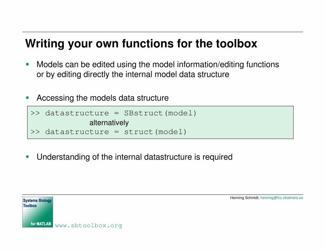
Writing your own functions for the toolbox
� Models can be edited using the model information/editing functionsor by editing directly the internal model data structure
� Accessing the models data structure
� Understanding of the internal datastructure is required
>> datastructure = SBstruct(model)alternatively
>> datastructure = struct(model)

Henning Schmidt, [email protected]
www.sbtoolbox.org
Writing your own functions for the toolbox
� Behind the scenes the model, before evaluation, is converted to one or more m-files
� An ODE description m-file is created by the functions
� An ODE file can be simulated using the standard MATLAB integrators
>> help SBcreateODEfile>> help SBcreateTempODEfile
>> SBcreateODEfile(model,’filename’)>> [t,x] = ode23s(’filename’,[0 100],filename)
Henning Schmidt, [email protected]
www.sbtoolbox.org
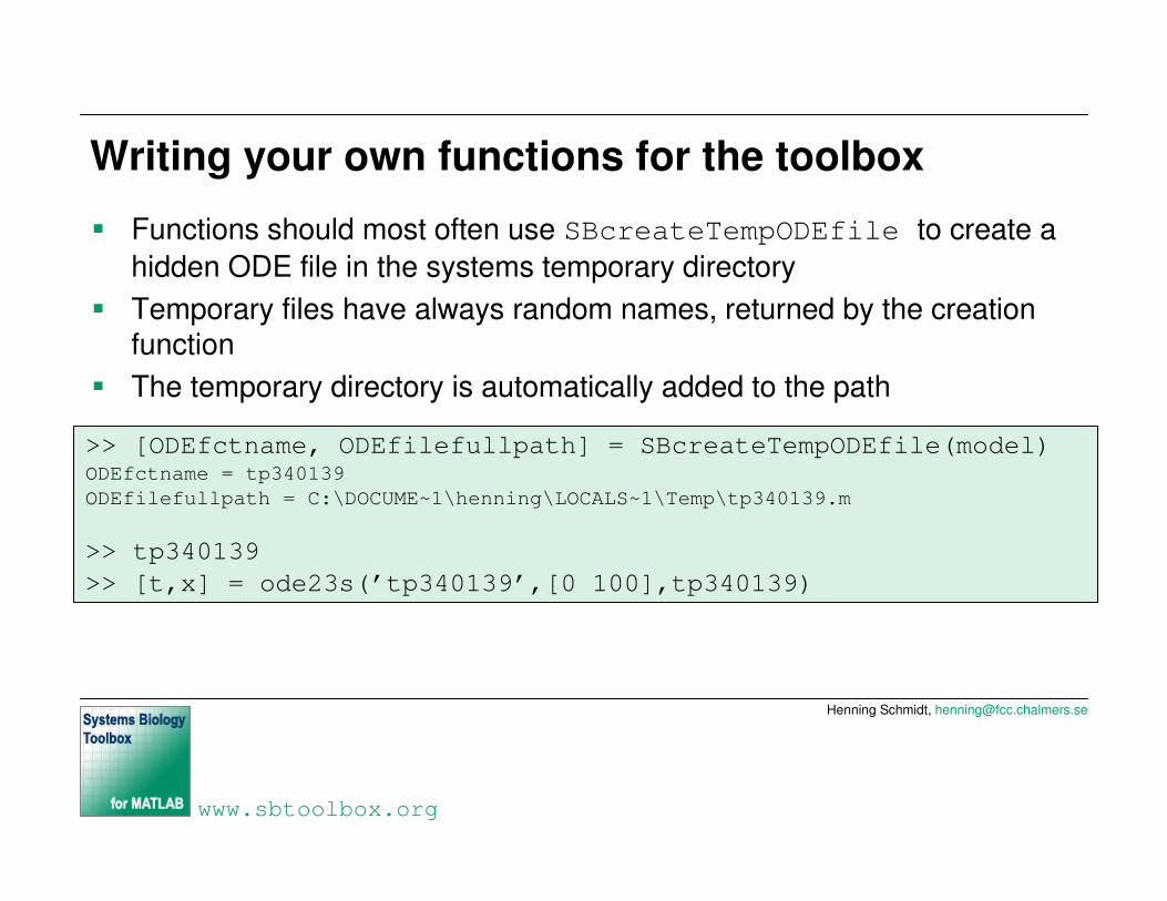
Writing your own functions for the toolbox
� Functions should most often use SBcreateTempODEfile to create a hidden ODE file in the systems temporary directory
� Temporary files have always random names, returned by the creation function
� The temporary directory is automatically added to the path
>> [ODEfctname, ODEfilefullpath] = SBcreateTempODEfile(model)ODEfctname = tp340139ODEfilefullpath = C:\DOCUME~1\henning\LOCALS~1\Temp\tp340139.m
>> tp340139>> [t,x] = ode23s(’tp340139’,[0 100],tp340139)

Henning Schmidt, [email protected]
www.sbtoolbox.org
Writing your own functions for the toolbox
� After use the temporary files should be deleted
� Deleting temporary files can be done using deleteTempODEfileSB it deletes � ODE m-file� Data file� Event files
>> deleteTempODEfileSB(ODEfilefullpath)
Henning Schmidt, [email protected]
www.sbtoolbox.org
Writing your own functions for the toolbox
� SBcreateODEfile and SBcreateTempODEfile do also create additional files on request� Event files
� Allowing to implement discrete state events� Data file
� Allowing to determine values of variables and reactions
>> help SBcreateODEfile>> help SBcreateTempODEfile

Henning Schmidt, [email protected]
www.sbtoolbox.org
Writing your own functions for the toolbox
� Some functions to have a look at: SBTOOLBOX/auxiliary
� Examples� deleteparameterSB� replaceelementSB� explodePCSB� ...
� andSB, orSB, piecewiseSB� unitstepSB, heavisideSB

Henning Schmidt, [email protected]
www.sbtoolbox.org
Writing your own functions for the toolbox
� Export of SBmodels to formats of other software packages
� An SBmodel is easily exported as a formatted textfile, implemented so far:� SBTOOLBOX/classes/@SBmodel/ ...
� SBcreateTEXTfile� SBcreateTEXTBCfile� SBcreateODEfile� SBcreateXPPAUTfile
� The user can easily write own export functions to other text based formats.� C/C++� JAVA� ...
Henning Schmidt, [email protected]
www.sbtoolbox.org
� Modifying existing MATLAB models for use with the toolbox

Henning Schmidt, [email protected]
www.sbtoolbox.org
Modifying existing MATLAB models
� Many, but not all functions in the toolbox can work with ODE m-files� The ODE m-files have some non-standard MATLAB features
� Adding this additional functionality to existing MATLAB models is straight forward
>> odefilename() % returns initial conditions
>> odefilename(’states’) % returns state names
>> odefilename(’parameters’) % returns parameter names
>> odefilename(’parametervalues’) % returns parameter values
Henning Schmidt, [email protected]
www.sbtoolbox.org
Modifying existing MATLAB models
� Best practice:
� Convert the m-files to SBmodel textual descriptions