Joint de ision making and ooperative solutions

Joint de ision making and ooperative solutionsProefs hriftter verkrijging van de graad van do tor aan TilburgUniversity, op gezag van de re tor magni� us,prof.dr. Ph. Eijlander, in het openbaar te verdedigenten overstaan van een door het ollege voor promotiesaangewezen ommissie in de aula van de Universiteit opvrijdag 13 januari 2012 om 14.15 uur doorEdwin Ruben Mauri e Antoine Lohmanngeboren op 29 mei 1985 te Beuningen.

Promotie ommissie:Promotor: prof. dr. Peter BormCopromotor: dr. Mar o SlikkerOverige leden: dr. Julio González-Díazprof. dr. Herbert Hamersprof. dr. Jean-Ja ques Heringsdr. Hans Reijniersedr. Tamás Solymosi

Joint de ision making and ooperative solutionsISBN 978 90 5668 305 4Copyright © 2011 Edwin LohmannAll rights reserved. No part of this publi ation may be reprodu ed or transmit-ted in any form or by any means ele troni or me hani al, in luding photo opying,re ording, or by any information storage and retrieval system, without permissionin writing from the author.

Orandum est ut sit mens sana in orpore sanoJuvenal, Satires

A knowledgementsI'm a lu ky man to ount on both handsthe ones I love. Pearl Jam, Just BreatheTo get a good impression of the years that lead to this dissertation, it is best totake a few steps ba k and look at it from a distan e. Sin e I de ided to go outWest (where the wind blows tall!), my distan e to Tilburg got pretty large. This,together with a personal habit to appre iate things even more on e they're behindme, makes me think this is a good time to re�e t on the past years. I'll start witha small synopsis: thank you, it's been great!The �rst of many thanks in this hapter should go out to the one that deservesit most: Peter Borm. In luding the se ond year proje t `zelfstandig modelleren',this is my �fth thesis supervised by Peter. He taught me the basi s of resear h,to be areful before saying `but that's straightforward'. But most importantly heintrodu ed me to game theory and sparked my enthusiasm for the subje t. For theResear h Master's thesis, Peter brought in Mar o Slikker as a se ond supervisor andhe stayed on board for the Ph. D. Thesis. I ouldn't have wished for a better super-vising team. It is great how the two of you were able to guide me in my resear h,motivate me whenever my enthusiasm was fading and help me out in the ongoingbattle to write everything down in a mathemati ally on ise way.I onsider myself really lu ky to have worked with a number of very pleasant oauthors. Stef Tijs and Marieke Quant helped out a lot with my �rst steps as avii

viii A knowledgementsresear her, also being the �rst steps of Alexia. I'm very happy with the resear hPeter and I arried out together with Jean-Ja ques, whi h is Chapter 3 in this the-sis. With his ideas and suggestions, Jean-Ja ques made the meetings in Tilburg andMaastri ht very valuable from a s ienti� point of view. Besides, lun h dis ussionswith Jean-Ja ques were always ni e (although... it really is pronoun ed `enniesee' !).I very mu h enjoyed the visit of Oriol Tejada to Tilburg as well as my return visitto Bar elona to write part of what is now Chapter 5. Resear h was never so frus-trating, but at the same time it has never been so mu h fun. Lastly, during thevisit of Julio González-Díaz to Tilburg, Ruud Hendri kx and I worked with him on ompleting the big matrix of Chapter 6. Initially, the subje t of our resear h wasnew to me and working together ould have been a little intimidating. However,thanks to their patien e and willingness to explain I got familiar with the subje tqui kly. Together with Peter, Mar o, Jean-Ja ques and Julio, the ommittee on-sists of Tamás Solymosi, Hans Reijnierse and Herbert Hamers. Thank you all fortaking the time to read the thesis and providing suggestions for improvement.John and Mireille, I appre iate that you agreed to be my paranymphs. It feelsgreat to know that the two of you have my ba k during the defense. I guess you areused to stand around for some time while I'm talking (a lot), too bad you'll have todo without a beer or a mojito this time.Se ond part of the job of a Ph. D. student is tea hing. I'm glad that besides ashort, but ni e sidestep to Probability & Statisti s, I ould keep tea hing the oursesI taught as a tea hing assistant during my studies. It was great to be working to-gether with Dolf Talman, Hans Reijnierse, and a long list of tea hing assistants.However, these ourses are not in the same league as the third ourse I've beentea hing over the last years: International Orientation. It's a bit of an unfair om-petition with the other ourses, as this ourse allowed me to go to Japan, Brazil andVietnam. Thanks to the people at Asset | First International for asking John andme year after year to supervise these study trips. Also, on e again a `thank you' toJohn, this time for involving me in this ourse and being a good travel mate on thetrips.This leads me to the third part of the job as a Ph. D. student: the annual onfer-en es. The basi idea here is to go to some foreign ity to present and dis uss your

A knowledgements ixwork, to meet fellow resear hers and to get inspiration for future resear h. Fortu-nately, it is easy to add a few days and enjoy the ity and the weather a bit with afew olleagues. Gerwald, John, Marloes, Mirjam, Soesja and Ruud: thanks for thegood ompany.A spe ial thanks goes out to Romeo, my o� e mate for all my Ph. D. years. Itwas ni e to share the good and bad times aused by resear h and tea hing. Also,thanks for having a good taste for musi so I ould play the musi I liked and intro-du ed me to a few artists you liked.The people I've mentioned so far have all had a dire t ontribution to my disser-tation. However, many other people had a positive in�uen e the past years. One ofthe reasons I've enjoyed the years as a Ph. D. student at Tilburg University so mu h,is the atmosphere in the department. Lun h together in an i y mensa, elebratingSinterklaas, playing boardgames: it was fun! Thanks Edwin, Elleke, Henk, Herbert,John, Lisanne, Marieke, Mirjam, René, Ruud, Peter, Salima and Willem.In my spare time I spent quite a few hours on a ra ing bike. I'm not a big fan oflong lonesome rides and thanks to the people at T.S.W.V De Meet, there were plentypeople to team up with. Bjorn, Camiel, Dennis de Dreu, Dennis Martens, Eri , Gijs,Matthijs, Paul, Stefan, and Thijs: thanks to you guys I wasn't like Boudewijn deGroot's lonesome rider all too often. The year I spent as the treasurer for the DeMeet might not have been the smoothest one, but I ertainly have learned manythings from it. Thanks Matthijs (from inside the board) and Thijs (from outside)for the support. Biking is fun, biking in the mountains is quite great. I spent a lotof my days o� in and around Oz-en-Oisans biking with friends and the people wewere guiding. These trips were a great su ess, on and o� the bike. A big thankyou to all my travel ompanions!A few people don't belong to any ategory mentioned above. However, they have ontributed in a very important way to my thesis simply by being a good friend tome, making me feel good and enjoying life in general in the last years. I want tomention Dennis, Mathijs, Ramon, Iris, Maaike and Gerben spe i� ally. These yearswould not have been nearly that great without you. Véronique and Mireille, youbelong to this list too. Although you are very di�erent, I still an't settle the old

x A knowledgementsdispute of `who's the most favourite sister?'. Thanks for all the support and all thefun over the years.Finally, Marga en Ewald, this thesis is in some way the end produ t of abouttwenty years of edu ation, whi h I wouldn't have ompleted without a lot of supportfrom you. Thanks for giving me the freedom to go the dire tion I wanted, but atthe same time stimulating me to do things in the right way.Devon, November 2011

Contents1 Introdu tion 12 Preliminaries 72.1 Basi mathemati al notation . . . . . . . . . . . . . . . . . . . . . . . 72.2 Cooperative game theory . . . . . . . . . . . . . . . . . . . . . . . . . 83 The Alexia value 113.1 Introdu tion . . . . . . . . . . . . . . . . . . . . . . . . . . . . . . . . 113.2 The Alexia value . . . . . . . . . . . . . . . . . . . . . . . . . . . . . 133.3 The Alexia value on lasses of games . . . . . . . . . . . . . . . . . . 193.3.1 Convex games . . . . . . . . . . . . . . . . . . . . . . . . . . . 213.3.2 Strongly ompromise admissible games . . . . . . . . . . . . . 223.3.3 Clan games . . . . . . . . . . . . . . . . . . . . . . . . . . . . 243.3.4 Compromise stable games and exa ti� ation . . . . . . . . . . 263.4 The reverse Alexia value and other modi� ations . . . . . . . . . . . 304 Minimal exa t balan edness 354.1 Introdu tion . . . . . . . . . . . . . . . . . . . . . . . . . . . . . . . . 354.2 Balan edness . . . . . . . . . . . . . . . . . . . . . . . . . . . . . . . 374.3 Exa t balan edness . . . . . . . . . . . . . . . . . . . . . . . . . . . . 404.4 Partitioning the lass of minimal exa t balan ed olle tions . . . . . . 464.5 Su� ient onditions for exa tness . . . . . . . . . . . . . . . . . . . . 524.A Minimal exa t balan ed olle tions . . . . . . . . . . . . . . . . . . . 604.A.1 N = {1, 2, 3} . . . . . . . . . . . . . . . . . . . . . . . . . . . 604.A.2 N = {1, 2, 3, 4} . . . . . . . . . . . . . . . . . . . . . . . . . . 61xi

xii Contents5 Mat hing situations: onne ting assignment and permutation 675.1 Introdu tion . . . . . . . . . . . . . . . . . . . . . . . . . . . . . . . . 675.2 A unifying model . . . . . . . . . . . . . . . . . . . . . . . . . . . . . 705.3 Assignment versus permutation . . . . . . . . . . . . . . . . . . . . . 745.3.1 Assignment games versus permutation games . . . . . . . . . 745.3.2 Böhm-Bawerk mat hing . . . . . . . . . . . . . . . . . . . . . 795.4 Permutation situations and games . . . . . . . . . . . . . . . . . . . . 885.4.1 The ore and exa tness . . . . . . . . . . . . . . . . . . . . . . 895.4.2 `Homogeneous alternatives' permutation . . . . . . . . . . . . 946 Sequen ing situations with Just-in-Time arrival, and related games1016.1 Introdu tion . . . . . . . . . . . . . . . . . . . . . . . . . . . . . . . . 1016.2 JiT sequen ing situations . . . . . . . . . . . . . . . . . . . . . . . . . 1046.3 JiT sequen ing games . . . . . . . . . . . . . . . . . . . . . . . . . . . 1136.A Proof of Lemma 6.3.2 . . . . . . . . . . . . . . . . . . . . . . . . . . . 1257 A taxonomy of rankings in tournaments 1317.1 Introdu tion . . . . . . . . . . . . . . . . . . . . . . . . . . . . . . . . 1317.2 Tournaments and ranking methods . . . . . . . . . . . . . . . . . . . 1347.3 Basi properties . . . . . . . . . . . . . . . . . . . . . . . . . . . . . . 1407.4 Response to vi tories and losses . . . . . . . . . . . . . . . . . . . . . 1467.5 S ore onsisten y . . . . . . . . . . . . . . . . . . . . . . . . . . . . . 1537.6 Monotoni ity . . . . . . . . . . . . . . . . . . . . . . . . . . . . . . . 1557.7 Dis ussion . . . . . . . . . . . . . . . . . . . . . . . . . . . . . . . . . 163Bibliography 165Author index 173Subje t index 175CentER dissertation series 179

Chapter 1Introdu tionGame theory is a bran h of mathemati s, des ribing and analyzing the intera tionamong de ision makers. Where de ision theory omprises the problem of �nding apreferred alternative when only one de ision maker is present, game theory assumesthe existen e of more than one de ision maker while the a tions of one de isionmaker possibly have an e�e t on the out ome for others. Central in game theory arethe on�i t situations arising from this intera tion. These on�i t situations an beof diverse nature, e.g., the fundamental on�i t situation of warfare, the evolutionof spe ies in biology, voting in politi s and pro�t sharing in e onomi s.The publi ation by Von Neumann (1928) laid the groundwork for game theory,but not before the book by Von Neumann and Morgenstern (1944) game theoryattra ted the attention of a wider audien e. Generally, game theory is divided intotwo main parts: non- ooperative game theory and ooperative game theory.In non- ooperative game theory, the involved parties, or players, a t in self-interest and the ompetitive nature of intera tion is dominant. A fo us is on �ndingrational out omes, equilibria: those strategy ombinations where none of the players an improve by unilaterally hanging his strategy. Ex ante the players annot makebinding agreements.In ooperative game theory, the main topi of this dissertation, the players areassumed to ooperate to a hieve an out ome preferred by the group as a wholeand the on�i t arises from dividing the jointly a hieved payo� stemming from thisout ome. So, the fo us is on sharing the pro�t obtained from ooperation. Thetype of ooperative games onsidered in this thesis, are transferable utility games.In this framework, players are allowed to transfer utility, su h as money, from oneplayer to another. Contrary to the non- ooperative setup there is a me hanism,1

2 Chapter 1. Introdu tionsu h as a legal system, allowing the players ex ante to make binding agreements ondividing the joint payo�. An important modeling aspe t is an adequate translationfrom the on�i t situation to a ooperative game, in whi h one expli itly de�nes the apabilities of subgroups of the players. A solution on ept assigns an allo ationto ea h game in a lass of transferable utility games. To divide the joint pro�ts,multiple solution on epts have been developed to apture di�erent notions of theidea of a `fair' allo ation. A entral notion is the ore, the set of those allo ationsfor whi h no group of players has an in entive to split o�.A spe i� area of appli ation, as dis ussed in this thesis, is joint de ision makingwithin the �eld of operations resear h. Operations resear h deals with optimizationproblems in business and industry, often with a ombinatorial aspe t. When di�er-ent players are involved in the de ision making pro ess or in the exe ution of tasks,we enter the area of operations resear h games.This thesis an roughly be divided into three parts. After the preliminaries, Chap-ter 3 and 4 of this dissertation ontain ontributions to the theory of transferableutility games in general. Then, the next two hapters analyze spe i� ooperativesituations originating from operations resear h problems. The last hapter is some-what of an outlier as it does not involve transferable utility games but provides ataxonomy of rankings in tournaments.As mentioned before, in ooperative game theory a number of solution on eptsattra ted attention. The Shapley value, the nu leolus and the ompromise valueare three of these well-studied solution on epts. For games with a non-empty ore Chapter 3, whi h is based on Tijs et al. (2011), introdu es an alternative tothese on epts alled the Alexia value. This solution on ept is de�ned via so- alledlexinals. Given an ordering on the set of players, the orresponding lexinal is su hthat every player takes the maximum he an obtain, respe ting the restri tions ofthe ore and the amounts already allo ated to his prede essors. Subsequently, toobtain the Alexia value one averages all lexinals.The Alexia value is analyzed for several lasses of games. Sin e the Alexia valuedepends on the game through its ore only, we fo us on lasses of games for whi hthe ore has a ni e stru ture. A key on ept in this analysis is ompromise stability:for sub lasses of the lass of ompromise stable games su h as strongly ompromiseadmissible games and big boss games, we show that the Alexia value oin ides with

3the nu leolus. Also, we relate the Alexia value to on epts originating from thetheory of bankrupt y situations.A transferable utility game is alled exa t if there exists for every oalition, anallo ation in the ore su h that this oalition re eives exa tly their value in the game.To he k for exa tness of a game, Csóka et al. (2011) introdu ed the equivalent on ept of exa t balan edness. Chapter 4, whi h is based on Lohmann et al. (2011),introdu es minimal exa t balan ed olle tions as those exa t balan ed olle tions,for whi h no proper subset exists that is also exa t balan ed. We show that all otherexa t balan ed olle tions are redundant for determining exa tness of the game. Thissigni� antly redu es the number of onditions to be he ked for exa tness. An exa tbalan ed olle tion not ontaining the grand oalition is minimal exa t if and onlyif the orresponding exa t balan ed weight ve tor is unique. On the other hand, anexa t balan ed olle tion ontaining the grand oalition is minimal exa t if and onlyif all orresponding exa t balan ed weight ve tors impose an equivalent onditionon the game.Furthermore, it is shown that the lass of minimal exa t balan ed olle tions an be partitioned into three types. The �rst type is the lass of minimal balan ed olle tions. The se ond type is formed by those olle tions that an be obtainedfrom a minimal balan ed olle tion by repla ing one oalition, with a weight stri tlysmaller than one, by its omplement. Finally, the third type is formed by all minimalbalan ed olle tions for every proper subgame, to whi h two oalitions are added:the grand oalition of the subgame, and the grand oalition of the original game.Chapter 5, whi h is based on Tejada et al. (2011), dis usses a general frameworkfor games derived from a non-negative, square matrix in whi h every entry representsthe value obtained from ombining the orresponding row and olumn. We assumethat every row and every olumn is asso iated with a player, where every playeris asso iated to at most one row and at most one olumn simultaneously. In thespe ial ase that every player is asso iated with one row or one olumn only, themodel boils down to the assignment problem ( f. Shapley and Shubik (1972)), in thespe ial ase that every player is asso iated with both a olumn and a row, the model orresponds to the permutation problem ( f. Tijs et al. (1984)). Within the generalframework, we an asso iate every assignment problem to a permutation problem.We show how all extreme points of the ore of the related permutation game an be

4 Chapter 1. Introdu tionviewed as extreme points of the ore of the underlying assignment game. Althoughin general not all extreme points of the underlying assignment game are overed inthis way, we prove that this is the ase within the spe ial lass of Bohm-Bawerkassignment games.In the last part of Chapter 5 the attention is shifted to permutation situationsand games only. We study the stru ture of the set of all matri es that lead topermutations games with the same ore. Moreover, we study a spe i� sub lass ofpermutation situations alled `homogeneous alternatives' permutation situations inwhi h the value obtained by a player while ombining his row with the olumn ofanother player is independent of the olumn player.In sequen ing situations a number of jobs have to be pro essed on one or morema hines, in su h a way that a ost riterion is minimized. For one-ma hine sequen -ing situations where the ost in urred by a job is a linear fun tion of its ompletiontime, the order minimizing total osts is su h that the jobs are pro essed in a non-in reasing order with respe t to their urgen y ( ost per time unit divided by thelength of the job, f. Smith (1956)). Curiel, Pederzoli, and Tijs (1989) initiated thegame theoreti study of this type of operations resear h games.Chapter 6, whi h is based on Lohmann et al. (2010), extends the literature onsequen ing games. We introdu e the model of sequen ing situations with Just-in-Time (JiT) arrival. Comparing with the standard sequen ing model, this model hastwo distin t features. First, instead of waiting in a queue from the moment the �rstjob starts, a job arrives at the fa tory as soon as its prede essor is �nished. Se ond,we introdu e a setup time: in between jobs, the ma hine should be adjusted forthe next job. The setup time we introdu e in our model is taken to depend on theprede essor only, so the time between �nishing a job and the start of the pro essingof the next job, does not depend on the job that is pro essed next. We restri tourselves to those situations with JiT arrival, where two values for the setup timeand two values for the ost parameter are allowed.We dis uss sequen ing situations with JiT arrival from two perspe tives. First,from an operations resear h perspe tive we solve the optimization problem regardingthe joint ost of all players. Se ond, we use the setting of ooperative game theoryto analyze the problem of dividing the osts of the optimal order among the players.We show that the ore of a JiT sequen ing game is always non-empty, and for large lasses of JiT sequen ing games we provide expli it expressions for both the ore

5and the nu leolus. Also, we introdu e a JiT sequen ing spe i� allo ation rule thatprovides a ore element.Chapter 7, whi h is based on González-Díaz et al. (2011), onsiders the problemof ranking a number of alternatives on the basis of information on pairwise ompar-isons of the alternatives. The set of alternatives along with the matrix ontainingthe, possibly partial, information on the pairwise omparisons is alled a tourna-ment. Tournaments are dis ussed in the literature on a variety of subje ts su h asstatisti s, psy hology, so ial hoi e and voting. Whereas the literature on tourna-ments usually assumes that the result of a pairwise omparison is binary, we assumethat the result of a omparison between two alternatives is a pair of non-negative re-als adding up to one, representing the result of both alternatives in the omparison.Hen e, the model is able to apture more general measures of relative strength.For this general setup, we provide a taxonomy of (the natural extensions of) ommon ranking methods for tournaments in the literature, and a new rankingmethod alled re ursive Bu hholz on the basis of properties. We use terminologyand interpretation from sports ompetitions for expositional purposes, our resultsare ontext free. In the pro ess, we provide an adaptation of the hara terization ofthe fair bets ranking method in Slutzki and Volij (2005) to our setting.

Chapter 2PreliminariesIn these preliminaries, we introdu e the basi mathemati al notation that is usedthroughout this dissertation. Also, we introdu e ooperative games and the mainsolution on epts.2.1 Basi mathemati al notationThroughout this dissertation, N denotes a �nite player set. We denote by 2N thepowerset of N , i.e., the olle tion of all subsets of N . Also, N = 2N\{∅} denotesthe olle tion of non-empty subsets of N . For every S ∈ N , the indi ator ve toreS ∈ RN is su h that eSi = 1 if i ∈ S and eSi = 0 if i ∈ N\S. An order σ of N isa bije tive fun tion σ : {1, ..., |N |} → N , where σ(k) denotes the player at positionk ∈ {1, ..., |N |} in the order σ. The set of all orders of N is denoted with Π(N).Given σ ∈ Π(N), we will use the notation σ for the reverse order: σ(1) = σ(|N |),σ(2) = σ(|N | − 1),..., σ(|N |) = σ(1).Given a polytope P ⊆ Rn, a ve tor x ∈ P is an extreme point if there are nox′, x′′ ∈ P , x′ 6= x′′ su h that x = 1

2x′ + 1

2x′′. For a polytope P , let ext(P ) denotethe set of extreme points, let int(P ) denote the relative interior and let dim(P )denote the dimension. For a polytope P of dimension n, a fa et is an (n − 1)-dimensional fa e. The Eu lidean distan e between two points x, y ∈ Rn is given by

d(x, y) =√

(x1 − y1)2 + ...+ (xn − yn)2. For x ∈ Rn, the open ball with enter xand radius ε is given by Bε(x) = {y ∈ Rn | d(x, y) < ε}.7

8 Chapter 2. Preliminaries2.2 Cooperative game theoryA transferable utility (TU) game (N, v) is de�ned by a �nite player set N and afun tion v on the set 2N of all subsets of N assigning to ea h oalition S ∈ 2N avalue v(S), des ribing the pro�t for the players in S when this oalition is formed.By onvention, v(∅) = 0. The lass of TU games with player set N is denoted byTUN . When no onfusion an arise, we denote v for (N, v) ∈ TUN .An allo ation is a ve tor x ∈ RN where for every i ∈ N , xi denotes the worthallo ated to player i. For the game v ∈ TUN , an allo ation x ∈ RN is alled e� ientif∑i∈N xi = v(N).The imputation set I(v) of a game v ∈ TUN is given by all individually rationaland e� ient allo ations, so

I(v) = {x ∈ RN |∑

i∈N

xi = v(N), xi ≥ v({i}) for all i ∈ N}.For a game v ∈ TUN the ore C(v) (Gillies (1953)) is de�ned as the set of thosee� ient allo ations of v(N), for whi h no oalition has an in entive to split o�:C(v) =

{x ∈ RN |

∑

i∈N

xi = v(N),∑

i∈S

xi ≥ v(S) for all S ∈ N}.A game is alled balan ed if its ore is non-empty ( f. Bondareva (1963), Shapley(1967)). The lass of balan ed games with player set N is denoted by ΓN . For agame (N, v) and oalition S ∈ 2N , the subgame (S, vS) is given by vS(T ) = v(T )for every T ∈ 2N . A game v ∈ TUN is alled totally balan ed if the ore of everysubgame is non-empty.For a game v ∈ TUN the utopia ve tor M(v) ∈ RN is given by:

Mi(v) = v(N)− v(N\{i}),for every i ∈ N , and the ve tor of minimum rights is given by:mi(v) = max

S:i∈S

{v(S)−

∑

j∈S\{i}

Mj(v)},for all i ∈ N . For a game v ∈ TUN the ore- over CC(v) (Tijs and Lipperts (1982))is de�ned as the set of those e� ient allo ations of v(N), where every player re eivesat least his minimum right and at most his utopia demand:

2.2. Cooperative game theory 9CC(v) =

{x ∈ RN |

∑

i∈N

xi = v(N), m(v) ≤ x ≤M(v)},It is readily veri�ed that C(v) ⊆ CC(v). For a game v ∈ TUN , the Weber set(Weber (1988)) is the onvex hull of all marginal ve tors:

W (v) = onv{mσ(v) | σ ∈ Π(N)},where for an order σ ∈ Π(N), the marginal ve tor mσ(v) ∈ RN is formed by themarginal ontributions with respe t to σ:mσ

σ(k)(v) = v({σ(1), σ(2), ..., σ(k)})− v({σ(1), σ(2), ..., σ(k − 1)}),for every k ∈ {1, ..., |N |}.A game v ∈ TUN is additive if for some a ∈ RN , v(S) =∑i∈S ai for all S ∈ N . Agame v ∈ TUN is alled onvex (Shapley (1971)) ifv(S ∪ {i})− v(S) ≤ v(T ∪ {i})− v(T ),for all i ∈ N , S ⊆ T ⊆ N\{i}. Convex games are those games for whi h the Weberset and the ore oin ide ( f. Shapley (1971), I hiishi (1981)).A solution on ept de�ned on Σ ⊆ TUN assigns an allo ation to ea h game v ∈ Σ.So, a solution on ept ould be de�ned on a subset of all TU-games only. Note thatwe de�ne solution on epts as being single-valued. Throughout this dissertationthe Shapley value, the ompromise value and the nu leolus are often used solution on epts.For a game v ∈ TUN the Shapley value Φ(v) (Shapley (1953)) is de�ned byΦ(v) =

1

|N |!

∑

σ∈Π(N)

mσ(v).We de�ne the ex ess of oalition S ∈ N with respe t to allo ation x ∈ I(v) byE(S, x) = v(S) −

∑i∈S xi. The ex ess measures the dissatisfa tion of oalition Swith respe t to allo ation x. Let ω(x) ∈ R2|N| be the ve tor of ex esses of x ∈ I(v),arranged in weakly de reasing order. For x, y ∈ Rn, x is lexi ographi ally smaller

10 Chapter 2. Preliminariesthan y, denoted by x ≤L y, if x = y or if there exists some k ∈ {1, ..., n} su h thatxi = yi for every i ∈ {1, ..., k − 1} and xk < yk.For ea h game (N, v) su h that I(v) 6= ∅, the nu leolus η(v) (S hmeidler (1969)) isde�ned as the unique allo ation x ∈ I(v) su h that ω(x) ≤L ω(y) for every y ∈ I(v).For every game v ∈ ΓN we have η(v) ∈ C(v).For a game v ∈ TUN su h that CC(v) 6= ∅, the ompromise value τ(v) (Tijs(1981)) is the unique e� ient ombination of the utopia ve tor and the ve tor ofminimum rights. For every i ∈ N :

τi(v) = aM(v) + (1− a)m(v),where a ∈ [0, 1] is su h that ∑i∈N τi(v) = v(N).We introdu e a number of standard properties for solution on epts: e� ien y,relative invarian e with respe t to strategi equivalen e, symmetry and dummy. Letψ be a solution on ept de�ned on Σ ⊆ TUN .The solution on ept ψ satis�es e� ien y on the domain Σ if∑i∈N ψi(v) = v(N)for every v ∈ Σ.Two games v ∈ TUN and w ∈ TUN are strategi ally equivalent (Tijs (1976))if there exist a ve tor a ∈ RN and a positive real number k su h that w(S) =

kv(S)+∑

i∈S ai for every S ∈ 2N . The solution on ept ψ satis�es relative invarian ewith respe t to strategi equivalen e on the domain Σ if ψ(w) = kψ(v) + a for allv, w ∈ Σ su h that w(S) = kv(S) +

∑i∈S ai for every S ∈ 2N and for some positivereal number k and ve tor a ∈ RN .Two players i ∈ N and j ∈ N are symmetri in the game v ∈ TUN if v(S∪{i}) =

v(S ∪ {j}) for every S ⊆ N\{i, j}. The solution on ept ψ satis�es symmetry onthe domain Σ if, for all v ∈ Σ, ψi(v) = ψj(v) for every i ∈ N and j ∈ N that aresymmetri in v.A player i ∈ N is a dummy in the game v ∈ TUN if v(S ∪ {i})− v(S) = v({i})for every S ⊆ N\{i}. The solution on ept ψ satis�es the dummy property on thedomain Σ if, for all v ∈ Σ, ψi(v) = v({i}) for every i ∈ N that is a dummy playerin v.

Chapter 3The Alexia value3.1 Introdu tionThis hapter, whi h is based on Tijs et al. (2011), introdu es the Alexia value, anew ore sele tor de�ned for ooperative games with a non-empty ore. Establishedone-point solution on epts su h as the Shapley value for general TU-games and the ompromise value for ompromise admissible TU-games, in general do not provide a ore-element. De�ned for TU-games that allow for e� ient and individually rationalallo ations, the nu leolus provides a ore-element for all games with a non-empty ore. In this respe t, the Alexia value provides an alternative to the nu leolus.The idea underlying the Alexia value is inspired by assignment problems, wherea number of obje ts are to be allo ated among an equal number of agents. One ofthe methods used to assign obje ts to agents is the so- alled serial di tatorship asdis ussed by e.g. Abdulkadiro�glu and Sönmez (1998) and Bogomolnaia and Moulin(2001). Given an ordering over the players, this me hanism assigns the �rst playerin the order his top hoi e, the se ond player is assigned his top hoi e among theremaining obje ts and so on. Of ourse, this method dis riminates between theagents, and to restore fairness the order is hosen randomly. As we are dealingwith transferable utility rather than obje ts, we an use the serial di tatorship toobtain an allo ation for every order of players, and average these allo ations. We an put numerous restri tions on the set of basi allo ations to hoose from. If weuse the Weber set - the onvex hull of all marginal ve tors - as this set of basi allo ations, this pro edure would lead to the Shapley value. In this hapter wewill on entrate on the basi set of e� ient and oalitionally stable allo ations, the ore. A similar approa h is also used in de�ning the `run-to-the-bank rule' (O'Neill11

12 Chapter 3. The Alexia value(1982)) for bankrupt y situations.This hapter de�nes the Alexia value via so- alled lexinals. Here a lexinal isde�ned as a lexi ographi al maximum of the ore, with respe t to an arbitrary orderon the players. Subsequently, to obtain the Alexia value one averages all lexinals.The Alexia value an be seen as a `run-to-the- ore rule' for games with a non-empty ore, as for every lexinal players are running to the ore a ording to a ertain order.Every player then takes the maximum he an obtain within the subset of the orethat remains after the players before him have made their respe tive hoi es.This way, the Alexia value ombines two often applied arguments with respe tto hoosing an allo ation: using orderings on the players, while at the same timerespe ting the fairness riterion of the ore. Hen e, it ombines attra tive propertiesof widely a epted allo ation rules su h as the Shapley value and the nu leolus and,in fa t, will oin ide with these solution on epts for several lasses of games. Anappli ation area of parti ular interest is formed by the lass of operations resear hgames. These games are used to divide ost savings stemming from operationsresear h problems with several de ision makers. The before mentioned propertiesas well as its intuitive nature make the Alexia value an attra tive allo ation rule:using, e.g., the appli ation area of �ow games, we show that the Alexia value anprovide an appealing alternative to both the nu leolus and the Shapley value.Sin e the Alexia value is based on the ore rather than on the game itself, itis interesting to analyze lasses of games where the ore has a ni e stru ture. For onvex games, those games where the marginal ontribution of a player in reases ifhe joins a larger oalition, the Alexia value and the Shapley value oin ide. Also, ompromise stability turns out to be an important notion with respe t to identifyingthe Alexia value. A game is alled ompromise stable (Quant et al. (2005)) if ithas a non-empty ore, and the ore oin ides with the ore over. Firstly, we showthat for the lass of strongly ompromise admissible games à la Driessen (1988),whi h form a spe i� sub lass of ompromise stable games (for whi h there is ahigh in entive to ooperate and form the grand oalition), the Alexia value and thenu leolus oin ide. Se ondly, we dis uss the Alexia value of lan games, whi h alsoform a sub lass of ompromise stable games. Clan games (Potters et al. (1989))are games with a nonempty oalition alled the lan, of whi h every member hasveto-power, and where it is more pro�table for the other players to unite in thenegotiations than to form smaller oalitions. For lan games, an expli it expressionfor the Alexia value is derived. For big boss games (Muto et al. (1988)), the sub lass

3.2. The Alexia value 13of lan games for whi h the lan onsists of one player only, the Alexia value again oin ides with the nu leolus. For any game with a non-empty ore, the exa ti� ationis de�ned as the unique exa t game with the same ore. Hen e, by de�nition theAlexia value of a game with a non-empty ore and of its exa ti� ation oin ide. Weuse the exa ti� ation to show that the Alexia value of a ompromise stable game oin ides with the ompromise extension of the run-to-the-bank rule for bankrupt ysituations as introdu ed by Quant et al. (2006).Finally, we introdu e the reverse Alexia value, whi h averages over the lexi o-graphi minima of the ore. This approa h an be seen as dual to the Alexia value:whereas the Alexia assumes that every player takes his restri ted maximum, thereverse Alexia assumes that every player is sent away with the minimum that hasto be allo ated to him, respe ting the restri tions of the ore and the amount al-ready allo ated to his prede essors. We show that for ompromise stable games and onvex games the Alexia value oin ides with the reverse Alexia value.The outline of this hapter is as follows. Se tion 3.2 introdu es the Alexia valueand dis usses some basi properties. Se tion 3.3 ontains the results on the Alexiavalue on spe i� lasses of games su h as onvex games, strongly ompromise ad-missible games and big boss games. Se tion 3.4 analyzes the reverse Alexia valueand we dis uss other possible modi� ations.3.2 The Alexia valueTo de�ne the Alexia value, we �rst introdu e the notion of a lexinal. Also, for thelexinals and for the Alexia value we provide a number of basi results. We show thatevery lexinal is an extreme point of the ore, but that there an exist extreme pointsthat are not a lexinal. We dis uss the Alexia value on 2-person games and stateseveral standard properties for solution on epts that are satis�ed by the Alexiavalue.De�nition 3.2.1 For (N, v) ∈ ΓN and an order σ ∈ Π(N), the lexinal λσ(v) ∈ RNis de�ned as the lexi ographi maximum on C(v) with respe t to σ, i.e.,λσσ(k)(v) = max

{xσ(k) | x ∈ C(v), xσ(l) = λσσ(l)(v) for all l ∈ {1, .., k − 1}

},for all k ∈ {1, ..., |N |}.

14 Chapter 3. The Alexia valueA lexinal is re ursively de�ned su h that every player gets the maximum he anobtain inside the ore under the restri tion that the players before him in the or-responding order obtain their restri ted maxima. It is readily he ked that everylexinal is an extreme point of the ore.Theorem 3.2.2 Let (N, v) ∈ ΓN . Then for every σ ∈ Π(N), λσ(v) is an extremepoint of the ore.Proof: Let σ ∈ Π(N). By onstru tion, λσ(v) ∈ C(v). Assume that σ ∈ Π(N)is su h that λσ(v) is not an extreme point of the ore. Then there exist x1, x2 ∈

C(v) with x1 6= x2 su h that λσ(v) = ax1 + (1 − a)x2 for some a ∈ (0, 1). Takel ∈ {1, ..., |N |} su h that x1σ(k) = x2σ(k) for every k ∈ {1, ..., l − 1} and x1σ(l) 6= x2σ(l).Without loss of generality we an assume x1σ(l) > x2σ(l). This means that

max{xσ(k) | x ∈ C(v), xσ(l) = λσσ(l)(v) for all l ∈ {1, .., k − 1}} ≥ x1σ(l) > λσσ(l),whi h ontradi ts the de�nition of a lexinal. Hen e, λσ(v) is an extreme point ofC(v). �However, for some games there exist extreme points of the ore that do not oin idewith a lexinal, whi h is shown in the next example. The game we onsider is avariant of an example in Derks and Kuipers (2002).Example 3.2.3 Let (N, v) be the game with N = {1, 2, 3, 4}, v({1}) = 1

2, v({2}) =

v({3}) = v({4}) = 0, andv(S) =

7 if |S| = 2,

12 if |S| = 3,

22 if S = N.For this example, we demonstrate how one an ompute the ore. In the remainder ofthis dissertation, we will omit the details of omputing the ore. Every ore-elementx ∈ C(v) satis�es the following system of (in)equalities:

3.2. The Alexia value 15x1 ≥ 1

2x2 + x4 ≥ 7

x2 ≥ 0 x3 + x4 ≥ 7

x3 ≥ 0 x1 + x2 + x3 ≥ 12

x4 ≥ 0 x1 + x2 + x4 ≥ 12

x1 + x2 ≥ 7 x1 + x3 + x4 ≥ 12

x1 + x3 ≥ 7 x2 + x3 + x4 ≥ 12

x1 + x4 ≥ 7 x1 + x2 + x3 + x4 = 22

x2 + x3 ≥ 7A ore-element x ∈ C(v) is an extreme point if in the above system 4 linearlyindependent (in)equalities hold with equality. As x1 + x2 + x3 + x4 = 22 holds forevery x ∈ C(v), we have at most (143

)= 364 andidate extreme points. For ea h ombination of three inequalities of the above system, we an he k if the equalities orresponding to these inequalities are linearly independent and he k if the resultingallo ation is a ore element. If both onditions hold, we obtained an extreme point ofthe ore. E.g., the equalities orresponding with x2 ≥ 0, x1 ≥ 1

2and x1+x2 ≥ 7 arelinearly dependent and therefore do not de�ne an extreme point. If the inequalities

x3 ≥ 0, x4 ≥ 0 and x2 + x4 ≥ 7 all hold with equality, we obtain the allo ationx = (15, 7, 0, 0). However, this is not a ore element, as x2 + x3 + x4 = 7 < 12.Now, if the inequalities x1 ≥ 1

2, x1 + x2 ≥ 7 and x1 + x4 ≥ 7 (for whi h the orresponding equalities are linearly independent) all hold with equality, we obtain

x = (12, 61

2, 81

2, 61

2). As this allo ation satis�es the above system of (in)equalities, xis an extreme point of the ore. Che king all ombinations results in the following

24 extreme points of the ore:(i) 12 extreme points whi h are permutations of (10, 5, 5, 2),(ii) 9 extreme points whi h are permutations of (7, 7, 8, 0) but with �rst oordinateunequal to 0,(iii) (12, 61

2, 61

2, 81

2), (1

2, 61

2, 81

2, 61

2) and (1

2, 81

2, 61

2, 61

2).Let σ ∈ Π(N). We have λσσ(1)(v) = max{xσ(1) | x ∈ C(v)} = 10. As every lexinal isan extreme point of the ore, λσ(v) is equal to a permutation of (10, 5, 5, 2). So, theextreme points given by (ii) and (iii) are not lexinals. ⊳

16 Chapter 3. The Alexia valueNow we an de�ne the Alexia value using the notion of a lexinal.De�nition 3.2.4 For (N, v) ∈ ΓN , the Alexia value α(v) is de�ned as the averageover the lexinals:α(v) =

1

|N |!

∑

σ∈Π(N)

λσ(v).Sin e every lexinal is a ore element, the average over all lexinals is also a oreelement. Hen e, for every (N, v) ∈ ΓN , α(v) ∈ C(v).The Alexia value ombines attra tive properties of both the nu leolus and theShapley value. First of all, just as the nu leolus, the Alexia value is a ore-sele torwhi h guarantees oalitional stability. Furthermore, just as the Shapley value av-erages over the marginal ve tor of every ordering, the Alexia value starts out bysele ting a ore allo ation for every ordering and averages over all these allo ations.The following example demonstrates the Alexia value, and shows that it oin ideswith the standard solution for 2-person games.Example 3.2.5 Let (N, v) ∈ ΓN with N = {1, 2}. Then v(N) ≥ v({1}) + v({2})and C(v) = onv{f 1, f 2} with f 1 = (v(N) − v({2}), v({2})), f 2 = (v({1}), v(N) −

v({1})). Clearly for the lexinals one �nds λ(1,2)(v) = f 1 and λ(2,1)(v) = f 2. So, theAlexia value α(v) = 12(f 1 + f 2) equals

(v({1}) + 1

2

(v(N)− v({1})− v({2})

), v({2}) +

1

2

(v(N)− v({1})− v({2})

)),the standard solution for the 2-person game (N, v). ⊳We show that the Alexia value satis�es a number of standard properties for solution on epts.Theorem 3.2.6 The Alexia value satis�es e� ien y, relative invarian e w.r.t.strategi equivalen e, symmetry and dummy on ΓN .Proof:E� ien y. Let (N, v) ∈ ΓN and σ ∈ Π(N). It holds that ∑i∈N λ

σi (v) = v(N) as∑

i∈N xi = v(N) for every x ∈ C(v) and λσ(v) ∈ C(v). Therefore, ∑i∈N αi(v) =1

|N |!

∑σ∈Π(N) λ

σ(v) = v(N).

3.2. The Alexia value 17Relative invarian e w.r.t. strategi equivalen e. Let (N, v) ∈ ΓN and (N,w) ∈ ΓNbe strategi equivalent. Take an additive game (N, a) and k ∈ R++ su h that w =

kv+a. Sin e x ∈ C(v) if and only if kx+a ∈ C(w), we have that λσ(w) = kλσ(v)+afor every σ ∈ Π(N) and therefore α(w) = kα(v) + a. So, the Alexia value satis�esrelative invarian e with respe t to strategi equivalen e.Symmetry. Let (N, v) ∈ ΓN , i ∈ N and j ∈ N be su h that i and j are symmetri in(N, v). Take x ∈ C(v) and let x be su h that xh = xh for every h ∈ N\{i, j}, xi = xjand xj = xi. Then x ∈ C(v). Hen e, for every σ ∈ Π(N) we have λσi (v) = λσ

′

j (v),where σ′(h) = σ(h) for every h ∈ N\{i, j}, σ′(i) = σ(j) and σ′(j) = σ(i). Therefore,αi(v) = αj(v) and we obtain that the Alexia value satis�es symmetry.Dummy. Let (N, v) ∈ ΓN and i ∈ N be su h that i is a dummy player in (N, v).As for every x ∈ C(v) we have xi = v({i}), we obtain λσi (v) = v({i}) for everyσ ∈ Π(N). Hen e, αi(v) = v({i}) so the Alexia value satis�es the dummy property.

�The properties mentioned in the theorem above are satis�ed by, e.g., the Shapleyvalue as well. A di�eren e between these solution on epts an be found in thefollowing hara terizations. A solution on ept ψ de�ned on the domain Σ ⊆ TUNsatis�es balan ed average ontributions on Σ if, for any (N, v) ∈ Σ with |N | ≥ 2 andany i ∈ N it holds that1

|N | − 1

∑

j∈N\{i}

(ψi(v)− ψi(vN\{j})) =1

|N | − 1

∑

j∈N\{i}

(ψj(v)− ψj(vN\{i})).The value ψi(v) − ψi(vN\{j}) an be seen as the ontribution of player j ∈ N toplayer i ∈ N , as the allo ation to player i in reases by ψi(v)−ψi(vN\{j}) be ause ofthe presen e of player j. The property of balan ed average ontributions says thatthe average ontribution of player i ∈ N to the other players equals the average ontribution of the other players to player i. Kongo et al. (2010) uses balan edaverage ontributions to hara terize the Shapley value.Theorem 3.2.7 (Kongo et al. (2010)) The Shapley value is the unique solution on ept on TUN that satis�es e� ien y and balan ed average ontributions.The Alexia value an be hara terized by similar properties. Let (N, v) ∈ ΓN with|N | ≥ 2. De�ne Ai(v) = max{xi | x ∈ C(v)} as the maximum payo� in the ore forplayer i ∈ N , and de�ne the Davis-Mas hler (DM) redu ed game (N\{i}, v−i) by

18 Chapter 3. The Alexia valuev−i(S) = max{v(S), v(S ∪ {i})− Ai(v)},for all S ⊆ N\{i}. Hen e, if (N, v) is onvex then (N\{i}, v−i) is the subgame of vwith respe t to player set N\{i}.The solution on ept ψ satis�es the balan ed average DM- ontributions on thedomain Σ ⊆ ΓN if, for all v ∈ Σ with |N | ≥ 2 and any i ∈ N ,

1

|N | − 1

∑

j∈N\{i}

(ψi(v)− ψi(v−j)) =

1

|N | − 1

∑

j∈N\{i}

(ψj(v)− ψj(v−i)).This property states that for every player i ∈ N , the average di�eren e between hispayo� in the original game and his payo� in the game where another player has anadvantageous position equals the average di�eren e between the payo� of the otherplayers in the original game and their payo� in the game where player i has anadvantageous position. This property an be used to hara terize the Alexia value.Theorem 3.2.8 (Kongo et al. (2010)) The Alexia value is the unique solution on ept whi h satis�es balan ed average DM- ontributions and e� ien y on thedomain ΓN .So, the Shapley value and the Alexia value are similar in the sense that bothsolution on epts balan e the average amount a player ontributes to another, butdi�er in the way these ontributions are measured. For the Shapley value, a player issent away with his marginal ontribution when forming the grand oalition, whereasfor the Alexia value this player obtains his maximum pay-o� in the ore of the game.The DM redu ed game an also be used to provide an alternative expression forthe Alexia value.Proposition 3.2.9 ( f. Caprari et al. (2008)) Let (N, v) ∈ ΓN . Then

αi(v) =1

|N |(Ai(v) +

∑

j∈N\{i}

αi(v−j)),for all i ∈ N .Proposition 3.2.9 states that the Alexia value an be omputed by averaging over |N |allo ations. In ea h of these allo ations one player j ∈ N is assigned his maximum ore payo� Aj(v), and the remainder v(N) − Aj(v) is allo ated a ording to theAlexia value of an appropriately de�ned game v−j on the remaining players inN\{j}.Note that if C(v) 6= ∅ then also C(v−j) 6= ∅, so the α(v−j) is indeed de�ned.

3.3. The Alexia value on lasses of games 193.3 The Alexia value on lasses of gamesFor several lasses of games, the Alexia value oin ides with either the Shapley valueor the nu leolus. First, we dis uss the lass of onvex games, where the Shapleyvalue equals the Alexia value. Se ondly, we fo us on two sub lasses of the lass of ompromise stable games: for strongly ompromise admissible games and big bossgames the Alexia value oin ides with the nu leolus. For lan games and simple�ow games we provide expli it expressions for the Alexia value. Finally, we useexa ti� ation to show that the Alexia value equals the ompromise extension of therun-to-the-bank rule.First of all, the di�eren es between the Alexia value and both the Shapley valueand the nu leolus are showed. The following example shows positive features of theAlexia value and its advantages over the nu leolus and the Shapley value in theappli ation area of �ow games as introdu ed by Kalai and Zemel (1982). We followthe slightly di�erent de�nition of Granot and Granot (1992).To des ribe a �ow network f we �rst need an undire ted graph G = (V,E). Theset of verti es V ontains two distinguished verti es: the sour e (So) and the Sink(Si). A �ow network is further des ribed by a apa ity fun tion: every edge e ∈ Ehas a nonnegative apa ity ap(e) ∈ R+. Lastly, every edge e ∈ E is owned by a oalition of players S(e) ∈ N . From the �ow network f , we obtain the �ow game vfby de�ning the value vf (S) of oalition S ∈ 2N as the amount that S an transportfrom sour e to sink, while utilizing only edges that are owned by the players in S.For simple �ow networks, it is assumed that every player owns exa tly one edgeand every edge has apa ity 1.So SiB

A1 24 3 5Figure 3.3.1: The simple �ow network f

20 Chapter 3. The Alexia valueExample 3.3.1 In the simple �ow network of Figure 3.3.1, all edges have apa ity1 and are undire ted. The players want to generate a �ow from the sour e Soto the sink Si. The number next to an edge denotes the player that owns theedge: e.g. player 4 owns the edge {So, A}. The player set is N = {1, ..., 5}. Forevery oalition S ⊆ N it an be omputed how mu h they an transport per timeunit from the sour e to the sink without using edges owned by players outside the oalition. This leads to the value vf (S) of the oalition S in the �ow game (N, vf) orresponding with the simple �ow network. One readily he ks that the ore of thisgame equals onv{(1, 0, 0, 1, 0), (0, 1, 0, 0, 1)}, while the Alexia value (and also thenu leolus) is given by α(vf ) = (1

2, 12, 0, 1

2, 12). Note that the Shapley value Φ(vf ) =

(2960, 2960, 115, 2960, 2960) lies outside the ore. Next, onsider the �ow network g (see Figure

So CBA D Si1 23 54 6Figure 3.3.2: The �ow network g), where all edges have apa ity 1 ex ept edges {C,D} and {D,Si} whi h have apa ity 2. This means that e.g. vg({1, 2, 5, 6}) = vg({3, 4, 5, 6}) = 1 and vg(N) = 2for the orresponding �ow game vg. Consider the allo ation x = (1

3, 13, 13, 13, 13, 13). Thehighest ex ess of x is −1

3whi h is attained at oalitions {1, 2, 5, 6}, {3, 4, 5, 6} and atall one-person oalitions. The ve tor of ex esses of this allo ation is lexi ographi allysmaller than the ve tor ex esses of any other element of the imputation set, as forevery x ∈ I(v), xi < 1

3for some i ∈ N . Hen e, η(vg) = (1

3, 13, 13, 13, 13, 13), while

α(vg) = Φ(vg) = (14, 14, 14, 14, 12, 12). The nu leolus allo ates vg(N) equally amongall players, although one ould argue that both the position in the graph and the apa ity of the edges of player 5 and 6 are superior to those of the other players.This dis repan y between the players is re�e ted in the Alexia value. ⊳The result in the �rst part of Example 3.3.1 an be generalized. For a �ow network

f , a ut is a oalition S ∈ 2N su h that no positive �ow an be generated from sour e

3.3. The Alexia value on lasses of games 21to sink without using at least one edge owned by S. So, S ∈ 2N is a ut in the �ownetwork f if vf (N\S) = 0. By Υf we denote the set of uts in the �ow network f .De�ne the set of minimum uts Υfmin = {S ∈ Υf | |S| ≤ |T | for every T ∈ Υf}. ByReijnierse et al. (1996), for a simple �ow network f we have C(vf ) = onv{eS | S ∈

Υfmin}. As every minimum ut ve tor onsists of the same number of ones and zeros,every minimum ut ve tor o urs the same number of times as lexinal. Therefore,

α(vf) equals the average over all minimal ut ve tors.Proposition 3.3.2 Let f be a simple �ow network. Thenα(vf ) =

1

|Υfmin|

∑

S∈Υfmin

eS.

3.3.1 Convex gamesFor the lass of onvex games, the Alexia oin ides with the Shapley value.Theorem 3.3.3 Let (N, v) be onvex. Then α(v) = Φ(v).Proof: Sin e (N, v) is onvex, C(v) = onv{mσ(v) | σ ∈ Π(N)} and, by Theorem3.2.2 , every lexinal is some marginal ve tor. In fa t, we will show that λσ(v) = mσ(v)for all σ ∈ Π(N). Let σ ∈ Π(N). By onvexity, v(N) − v(N\{i}) ≥ v(S) −

v(S\{i}) for all S ⊆ N\{i}, and hen e λσσ(1)(v) = maxx∈C(v) xσ(1) = mσσ(1)(v) using onvexity. Take k ∈ {2, ..., |N |}. Now assume that λσσ(j)(v) = mσ

σ(j)(v) for allj ∈ {1, ..., k − 1}. Take S = {σ(k + 1), ..., σ(|N |)}. Then ∑k−1

j=1 λσσ(j)(v) = v(N) −

v(S ∪ {σ(k)}). Sin e λσ(v) ∈ C(v), it must hold that ∑i∈S λσi (v) ≥ v(S). Hen e,

λσσ(k)(v) ≤ v(S∪{σ(k)})−v(S) = mσσ(k)(v). But asmσ(v) ∈ C(v) we know λσσ(k)(v) =

mσσ(k)(v). It now follows that α(v) = 1

|N |!

∑σ∈Π(N) λ

σ(v) = 1|N |!

∑σ∈Π(N)m

σ(v) =1

|N |!

∑σ∈Π(N)m

σ(v) = Φ(v). �The following theorem shows that the Alexia value is additive on the lass of onvexgames. Together with Theorem 3.3.3, this provides an alternative proof for theadditivity of the Shapley value on the lass of onvex games.Theorem 3.3.4 Let (N, v) and (N,w) be onvex games. Then α(v + w) = α(v) +

α(w).

22 Chapter 3. The Alexia valueProof: We have C(v) +C(w) = C(v+w), sin e C(v) =W (v), C(w) = W (w) andmσ

σ(k)(v + w) = v({σ(1), ..., σ(k)}) + w({σ(1), ..., σ(k)})

−v({σ(1), ..., σ(k − 1)})− w({σ(1), ..., σ(k − 1)})

= mσσ(k)(v) +mσ

σ(k)(w),for every k ∈ {1, ..., |N |}. This means that α(v+w) = α(v)+α(w), sin e λσ(v+w) =mσ(v + w) = mσ(v) +mσ(w) = λσ(v) + λσ(w) for every σ ∈ Π(N). �We now turn to several sub lasses of the lass of ompromise stable games, su h asstrongly ompromise admissible games and lan games.3.3.2 Strongly ompromise admissible gamesA game is alled ompromise admissible (also known as quasi-balan ed) if the ore over is non-empty. For a ompromise admissible game (N, v) one an hara terizethe ore over with the use of larginals. For all σ ∈ Π(N), the larginal ℓσ(v) isde�ned by

ℓσσ(k)(v) =

Mσ(k)(v) if k∑

j=1

Mσ(j)(v) +

|N |∑

j=k+1

mσ(j)(v) ≤ v(N),

mσ(k)(v) if k−1∑

j=1

Mσ(j)(v) +

|N |∑

j=k

mσ(j)(v) ≥ v(N),

v(N)−k−1∑

j=1

Mσ(j)(v)−

|N |∑

j=k+1

mσ(j)(v) otherwise,for all k ∈ {1, . . . , |N |}. For ea h ompromise admissible game (N, v) the ore over oin ides with the onvex hull of all larginal ve tors:CC(v) = onv{ℓσ(v) | σ ∈ Π(N)}.A ompromise admissible game (N, v) is alled ompromise stable (Quant et al.(2005)) if the ore over equals the ore.A ompromise admissible game (N, v) is alled strongly ompromise admissible( f. Driessen (1988)) if for all S ∈ N it holds that:

3.3. The Alexia value on lasses of games 23v(N)− v(S) ≥

∑

i∈N\S

Mi(v)Strongly ompromise admissible games are also alled dual simplex games or 1- onvex games. From Quant et al. (2005) it follows that every strongly ompromiseadmissible game is ompromise stable.Note that ompromise admissibility and strongly ompromise admissibility implyopposite onditions on the utopia demands. Compromise admissibility implies thatthe utopia demands are large: there exists an e� ient allo ation su h that everyplayer obtains at most his utopia demand. Strongly ompromise admissibility onthe other hand implies that the utopia demands are small: if a oalition is assignedexa tly its value, all players outside a oalition an obtain their utopia demands.In fa t, Driessen (1988) shows that for every strongly ompromise admissible game(N, v) it holds that v(N) =

∑j∈N\{i}Mj(v) +mi(v) for every i ∈ N .For our result on the Alexia value of strongly ompromise admissible games, weuse the following expressions for the ore and the nu leolus of strongly ompromiseadmissible games, derived by Driessen (1988).Theorem 3.3.5 ( f. Driessen (1988)) If (N, v) is strongly ompromise admissible,then(i) C(v) = onv {{M(v)eN\{i} +m(v)e{i}}i∈N

},(ii) η(v) = τ(v) = |N |−1|N | M(v) + 1

|N |m(v), the bary enter of C(v).For strongly ompromise admissible games, the Alexia value oin ides with the nu- leolus.Theorem 3.3.6 Let (N, v) be strongly ompromise admissible. Then α(v) =

η(v) = τ(v).Proof: Let (N, v) be strongly ompromise admissible. By part (i) of Theorem3.3.5, C(v) = onv{{M(v)eN\{i} +m(v)e{i}}i∈N}. Let σ ∈ Π(N). Then λσσ(k)(v) =

Mσ(k)(v) for all k ∈ {1, ..., |N | − 1}, and λσσ(|N |)(v) = mσ(|N |)(v). Therefore,0As an allo ation rule, the bary enter of the ore is known as the ore- enter. For a studyon the ore- enter, see e.g. González-Díaz and Sán hez-Rodríguez (2007) and González-Díaz andSán hez-Rodríguez (2009)

24 Chapter 3. The Alexia valueα(v) =

1

|N |!

∑

σ∈Π(N)

λσ(v)

=1

|N |!(|N |!− (|N | − 1)!)M(v) + ((|N | − 1)!)m(v)]

= η(v)

= τ(v),where the last equalities follow from Theorem 3.3.5 (ii). �3.3.3 Clan gamesClan games are introdu ed in Potters et al. (1989). Big boss games, whi h forma sub lass of lan games, are introdu ed in Muto et al. (1988) and are further onsidered in Branzei and Tijs (2001) and Tijs and Branzei (2002). For big bossgames, we show that the Alexia value oin ides with the nu leolus. This does nothold for the more general lass of lan games, but we obtain an expli it expressionfor the Alexia value on this lass of games.A game (N, v) is alled a lan game if v(S) ≥ 0 for all S ∈ 2N , M(v) ≥ 0 and ifthere exists a oalition C ∈ N alled the lan su h that:(i) Clan property: v(S) = 0 for all S with C 6⊆ S.(ii) Union property: v(N)− v(S) ≥∑

i∈N\S Mi(v) for ea h S ∈ 2N with C ⊆ S.Note that all players in C are symmetri in (N, v) as v(S) = 0 for every S ∈ 2N ,C 6⊆ S. A lan game (N, v) is alled a big boss game if there exists a lan C = {b}for some b ∈ N . The player b is alled the big boss.As is shown by Quant et al. (2005), lan games are ompromise stable. Howeverthey are not ne essarily strongly ompromise admissible.Example 3.3.7 Consider the lan game (N, v), de�ned by N = {1, 2, 3} andS {1} {2} {3} {1, 2} {1, 3} {2, 3} N

v(S) 0 0 0 5 0 0 10This game is a lan game with C = {1, 2}. Clearly, M(v) = (10, 10, 5). Thisgame is not strongly ompromise admissible, sin e v(N) − v({1}) = 10 < 15 =∑j∈N\{1}Mj(v). ⊳

3.3. The Alexia value on lasses of games 25Potters et al. (1989) provide an expli it expression for the ore of a lan game. Fora lan game (N, v) with lan C ∈ N , S ⊆ N\C and i ∈ C de�ne zS,i ∈ RN byzS,ij =

Mj(v) if j ∈ S,

v(N)−∑

h∈S

Mh(v) if j = i,

0 else,for all j ∈ N .Theorem 3.3.8(i) ( f. Potters et al. (1989)). Let (N, v) be a lan game with lan C ∈ N . ThenC(v) = onv{zS,i | S ⊆ N\C, i ∈ C}.(ii) ( f. Muto et al. (1988)). Let (N, v) be a big boss game with big boss b ∈ N .Then, for all i ∈ N ,ηi(v) =

12Mi(v) if i 6= b,

v(N)−1

2

∑

j∈N\{b}

Mj(v) if i = b.

Theorem 3.3.9 Let (N, v) be a big boss game. Then α(v) = η(v).Proof: Let player b ∈ N be the big boss. By Theorem 3.3.8 (i) with C = {b}, forall σ ∈ Π(N) and every k ∈ {1, ..., |N |} su h that σ(k) 6= b it holds thatλσσ(k)(v) =

{Mσ(k)(v) if k < σ−1(b),

0 if k > σ−1(b).Therefore, αi(v) =1

|N |!

∑σ∈Π(N) λ

σi (v) =

1|N |!Mi(v) · |{σ ∈ Π(N)|σ−1(i) < σ−1(b)}| =

12Mi(v) = ηi(v) for ea h i ∈ N\{b}. By e� ien y of η and α it then follows thatα(v) = η(v). �For lan games however, the Alexia value does not ne essarily equal the nu leolus.

26 Chapter 3. The Alexia valueExample 3.3.10 Consider the lan game of Example 3.3.7. We have η(v) =

(334, 33

4, 21

2). The ore is given by C(v) = onv{(5, 0, 5), (0, 5, 5), (10, 0, 0), (0, 10, 0)}.This implies that α(v) = 1

6· (25, 25, 10). ⊳The following theorem provides an expli it des ription of the Alexia value on the lass of lan games.Theorem 3.3.11 Let (N, v) be a lan game with lan C ⊆ N , |C| ≥ 2. Then, forall i ∈ N ,

αi(v) =

Mi(v)1+|C| if i ∈ N\C,

v(N)−∑

j∈N\CMj(v)

1+|C|

|C|if i ∈ C.Proof: By Theorem 3.3.8 (i), for all j 6∈ C it holds that

λσj (v) =

{Mj(v) if σ−1(j) < σ−1(i) for all i ∈ C,

0 else.Let j ∈ N\C. The number of orders where λσj (v) = Mj(v) equals |N |!|C|+1

, sin e in afra tion 1|C|+1

of a total of |N |! possible orders player j stands in front of all playersin the lan. This implies that αj(v) =Mj(v)

|C|+1for all j ∈ N\C. Sin e the Alexia valueis e� ient, the remainder is divided among the lan members. As lan members aresymmetri and the Alexia value satis�es symmetry, every lan member obtains anequal share of the remainder. �3.3.4 Compromise stable games and exa ti� ationTo obtain an expli it expression for the Alexia value on the lass of ompromisestable games we use exa ti� ation. A balan ed game (N, v) is alled exa t (S hmei-dler (1972)) if for every oalition S ⊆ N there exists an element x ∈ C(v) su hthat ∑i∈S xi = v(S). We refrain from a more elaborate dis ussion on the topi ofexa t games, as this is the topi of Chapter 4 of this dissertation. The exa ti� ation

(N, vE) of an arbitrary game (N, v) ∈ ΓN is the unique exa t game with the same ore as the original game v, i.e.,vE(S) = min

{∑

i∈S

xi | x ∈ C(v)},

3.3. The Alexia value on lasses of games 27for ea h S ⊆ N . So, C(vE) = C(v) for every (N, v) ∈ ΓN and vE = v if andonly if (N, v) is exa t. Note that if for two games (N, v) and (N,w) we haveC(v) = C(w) 6= ∅, then α(v) = α(w). Hen e, α is invariant with respe t to ex-a ti� ation: α(v) = α(vE) for every (N, v) ∈ ΓN . We use exa ti� ation to showthat for ompromise stable games, the Alexia value oin ides with the Shapley valueof the exa ti� ation. Moreover, within this lass of games the Alexia value equalsthe ompromise extension of the run-to-the-bank rule for bankrupt y situations.A bankrupt y situation is de�ned as a triple (N,E, d), where E ∈ R+ is theestate whi h has to be divided among a set of players N . The laim ve tor isdenoted by d ∈ RN

+ , where di represents the laim of player i ∈ N . It is assumedthat E ≤∑

i∈N di. With a bankrupt y situation one an asso iate a bankrupt ygame (N, vE,d), where the value of a oalition equals the amount of the estate not laimed by the players outside the oalition: vE,d(S) = max{0, E −

∑i∈N\S di

} forall S ⊆ N . Curiel et al. (1987) showed that every bankrupt y game is onvex and ompromise stable. O'Neill (1982) introdu es the run-to-the-bank (RTB) rule todivide the estate among the laimants.For a bankrupt y situation (N,E, d) the run-to-the-bank rule RTB(E, d) is givenbyRTB(E, d) =

1

|N |!

∑

σ∈Π(N)

rσ(E, d),where for all σ ∈ Π(N) and k ∈ {1, ..., |N |},

rσσ(k)(E, d) = max{min{dσ(k), E −

k−1∑

l=1

dσ(l)}, 0}.The interpretation of rσσ(k) is as follows: the players arrive at the bank a ording tothe order σ. Upon arrival, a player re eives his total laim or, if there is not enoughmoney left to satisfy his laim, the maximum amount that is available. Importantly,for every bankrupt y situation (E, d) it holds that RTB(E, d) = Φ(vE,d).The ompromise extension RTB* of the RTB-rule to the lass of all ompromiseadmissible games is introdu ed by Quant et al. (2006). For ea h ompromise ad-missible game (N, v), the ompromise extension RTB* of the RTB-rule is given by

RTB∗(v) = m(v) +RTB(v(N)−∑

i∈N

mi(v),M(v)−m(v)).

28 Chapter 3. The Alexia valueTheorem 3.3.12 Let (N, v) be ompromise stable. Then(i) (N, vE) is strategi ally equivalent to a bankrupt y game.(ii) α(v) = Φ(vE) = RTB∗(v).Proof:(i) Sin e (N, v) is ompromise stable, C(v) = CC(v). Hen e, for all S ⊆ N

vE(S) = min{∑

i∈S

xi | x ∈ C(v)}

= min{∑

i∈S

xi | x ∈ CC(v)}

= min{∑

i∈S

λσi (v) | σ ∈ Π(N)}

=∑

i∈S

λσ′

i ,where σ′ ∈ Π(N) is su h that σ′(k) ∈ N\S for all k ∈ {1, ..., |N\S|}. Therefore,vE(S) =

∑

i∈S

mi(v) if ∑i∈N\SMi(v) +∑

i∈Smi(v) ≥ v(N),

v(N)−∑

i∈N\S

Mi(v) if ∑i∈N\SMi(v) +∑

i∈Smi(v) < v(N).The �rst ase orresponds with the pivot of λσ′(v) (the �rst player in the order σ′that does not obtain his utopia demand) being a member of N\S, and the se ond ase orresponds with the pivot of λσ′

(v) being a member of S.Consider the bankrupt y problem (N,E, d) with E = v(N)−∑

i∈N mi(v) and di =Mi(v)−mi(v) for all i ∈ N . The orresponding bankrupt y game (N, vE,d) is givenby

vE,d(S) = max{0, v(N)−

∑

i∈N\S

Mi(v)−∑

i∈S

mi(v)},for all S ∈ 2N .Sin e vE = vE,d +m(v), (N, vE) is strategi ally equivalent to the game (N, vE,d).(ii) Be ause (N, vE) is strategi ally equivalent to a bankrupt y game, (N, vE) is onvex and ompromise stable. Sin e C(v) = C(vE), we have α(v) = α(vE). So,

3.3. The Alexia value on lasses of games 29with E = v(N)−∑

i∈N mi(v) and di =Mi(v)−mi(v) for all i ∈ N , the proof of (i)implies thatRTB∗(v) = m(v) +RTB(v(N)−

∑

i∈N

m(v),M(v)−m(v))

= m(v) + Φ(vE,d)

= Φ(vE,d +m(v)),where the se ond equality holds as RTB(E, d) and Φ(vE,d) oin ide for everybankrupt y situation. The last equality is obtained by additivity of Φ: Φ(v) +

Φ(w) = Φ(v + w) for every (N, v) and (N,w). Taking w = vE,d in the proof of part(i), we have

RTB∗(v) = Φ(vE)

= α(v),where the last equality holds by Theorem 3.3.3. �The previous theorem also provides an alternative proof for the fa t that for two andthree person games exa tness is equivalent to onvexity. For arbitrary N , onvexityimplies exa tness as every marginal ve tor is an element of the ore. Every exa tgame (N, v) is equal to its exa ti� ation (N, vE). Sin e every balan ed two or threeperson game is ompromise stable, this implies that (N, v) is strategi ally equivalentwith a bankrupt y game. As bankrupt y games are onvex, we obtain that (N, v)is onvex.On the lass of ompromise stable games, whi h ontains the lass of bankrupt ygames, one re ognizes an essential di�eren e between the Alexia value and the nu- leolus.To demonstrate this di�eren e, we �rst introdu e the Aumann-Mas hler rule AM .Given a bankrupt y situation (N,E, d), denote CEA(E, d) for the onstrained equalaward rule, given byCEAi(E, d) = min{a, di},for every i ∈ N , where a ∈ R+ is su h that ∑i∈N min{a, di} = E.Now the Aumann-Mas hler rule AM(E, d) (Aumann and Mas hler (1985)) isgiven by

30 Chapter 3. The Alexia valueAMi(E, d) =

CEAi(E,1

2d) if ∑j∈N dj ≥ 2E

di − CEAi(∑

j∈N

dj − E,1

2d) if ∑j∈N dj < 2Efor every i ∈ N .For a ompromise stable game (N, v), the Alexia value is given by:

α(v) = m(v) +RTB(v(N)−∑

i∈N

mi(v),M(v)−m(v)),whereas Quant et al. (2005) show thatη(v) = m(v) + AM(v(N)−

∑

i∈N

mi(v),M(v)−m(v)).So, the Alexia value and the nu leolus are similar in the sense that every playerobtains his minimum right, and the framework of a bankrupt y situation is used toallo ate the remainder. The di�eren e between the Alexia value and the nu leoluslies in the treatment of this bankrupt y situation: the Alexia value uses the run-to-the-bank rule whereas the nu leolus uses the Aumann-Mas hler rule to obtain anallo ation for the related bankrupt y situation.3.4 The reverse Alexia value and other modi� a-tionsThe de�nition of the Alexia value allows for modi� ations in a number of di�er-ent dire tions. Inspired by the literature on weighted Shapley values, Caprari et al.(2008) introdu es two weighted Alexia values. These weighted Alexia values di�er inthe way the weights are assigned to orders: for the so- alled µ-mixed lexi ographi value weights are assigned to orders dire tly, whereas for the p-weighted lexi o-graphi value weights are assigned to players and the p-weighted lexi ographi valueis the expe tation of the allo ation when players are sent away a ording to theirrelative weights. For every set of p-weights there exists a set of µ-weights su h thatthe p-weighted lexi ographi value and the µ-mixed lexi ographi value oin ide.Also, the p-weighted lexi ographi value is extended to the (p, S)-weighted lexi o-graphi value to ir umvent the ase where multiple players have zero p-weight.Caprari et al. (2008) generalizes a number of results mentioned in this hapter:for onvex games the (p, S)-weighted lexi ographi value oin ides with the (p, S)-weighted Shapley value (Kalai and Samet (1988)) and for big boss games, lan games

3.4. The reverse Alexia value and other modi� ations 31and strongly ompromise admissible games (whi h are all ompromise stable), the(p, S)-weighted lexi ographi value oin ides with the (p, S)-weighted Shapley valueon the exa ti� ation of the game.Here, we introdu e another modi� ation to the Alexia value. We introdu e thereverse Alexia value, the average over all lexi ographi al minima of the ore.De�nition 3.4.1 For (N, v) ∈ ΓN , the reverse Alexia value α(v) is given by

α(v) =1

|N |!

∑

σ∈Π(N)

λσ(v),where for all σ ∈ Π(N) the reverse lexinal λσ(v) ∈ RN is de�ned by

λσ

σ(k)(v) = min{xσ(k) | x ∈ C(v), xσ(l) = λ

σ

σ(l)(v) for all l ∈ {1, ..., k − 1}},for all k ∈ {1, ..., |N |}.Numerous results on lexinals and the Alexia value dis ussed before in this hapteralso hold for reverse lexinals and the reverse Alexia value. Every reverse lexinal isan extreme point of the ore, but for some games there exist extreme points of the ore that do not oin ide with a reverse lexinal. In Example 3.2.3, (10, 5, 5, 2) is anextreme point of the ore, but it is not a reverse lexinal. Using the same reasoningsas for the Alexia value, it is obtained that the reverse Alexia value satis�es theproperties of e� ien y, relative invarian e with respe t to strategi equivalen e,symmetry and dummy. As Example 3.4.4 shows that the Alexia value and thereverse Alexia value need not oin ide, it follows that the reverse Alexia value doesnot satisfy balan ed average DM- ontributions.It turns out that for ompromise stable games, the Alexia value and the reverseAlexia value oin ide.Theorem 3.4.2 Let (N, v) be ompromise stable. Then α(v) = α(v).Proof: As (N, v) is ompromise stable, C(v) = CC(v) 6= ∅. We showed that

α(v) = RTB∗(v) and, by Quant et al. (2006), we haveRTB∗(v) =

1

|N |!

∑

σ∈Π(N)

ℓσ(v).

32 Chapter 3. The Alexia valueTake σ ∈ Π(N). We show that λσ(v) = ℓσ(v). Clearly,λσ

σ(1)(v) = min{xσ(1) | x ∈ C(v)

}

= min{xσ(1) | x ∈ CC(v)

}.Sin e xσ(1) ≥ mi(v) and ∑

i∈N\σ(1) xi ≤∑

i∈N\{σ(1)}Mi(v), λσ

σ(1)(v) =

max{mσ(1), v(N) −∑

i∈N\{σ(1)}Mi(v)} = ℓσσ(1)(v). Now onsider k ∈ {2, ..., |N |}and assume that λσσ(l)(v) = ℓσσ(l)(v) for l ∈ {1, ..., k − 1}. Take S = {σ(1), ..., σ(k)}.Thenmin{

∑

i∈S

xi | x ∈ CC(v)} = max{v(N)−∑

i∈N\S

Mi(v),∑

i∈S

mi(v)},

=∑

i∈S

ℓσi (v),where the �rst equality follows from the de�nition of the ore- over: ∑i∈S xi ≥∑i∈Smi(v) and ∑i∈N\S xi ≤

∑i∈N\S Mi(v). So, if λσσ(l)(v) = ℓσσ(l)(v) for l ∈

{1, ..., k − 1} then λσ

σ(k)(v) = ℓσσ(k)(v). By indu tion it follows that λσ(v) = ℓσ(v).This leads toα(v) =

1

|N |!

∑

σ∈Π(N)

ℓσ(v) =1

|N |!

∑

σ∈Π(N)

ℓσ(v) = α(v),whi h on ludes the proof. �Note that the lass of ompromise stable games in ludes strongly ompromise ad-missible games and lan games. Hen e, most results derived in se tion 3 not onlyhold for the Alexia value, but for the reverse Alexia value as well. For onvex games,the reverse Alexia value oin ides with the Alexia value.Theorem 3.4.3 Let (N, v) be onvex. Then α(v) = α(v).Proof: Let σ ∈ Π(N). By indu tion on the position k ∈ {1, ..., |N |}, we prove thatλσ(v) = mσ(v). Consider the �rst player in the order:

λσ

σ(1)(v) = min{xσ(1) | x ∈ C(v)

}

= min{xσ(1) | x ∈ W (v)

}

3.4. The reverse Alexia value and other modi� ations 33Sin e v({i}) ≤ v(S ∪ {i})− v(S) for every S ∈ N , we haveλσ

σ(1)(v) = v({σ(1)})

= mσσ(1)(v).Now onsider k ∈ {2, ..., |N |} and, assume that λσσ(l)(v) = mσ

σ(l)(v) for l ∈ {1, ..., k−

1}. Thenk−1∑

l=1

λσ

σ(l)(v) =k−1∑

l=1

mσσ(l)(v) = v({σ(1), ..., σ(k − 1)}).Let S = {σ(1), ..., σ(k)}. By de�nition of the ore, min

{∑i∈S xi | x ∈ C(v)

}≥

v(S). Therefore, λσσ(k)(v) ≥ v(S)− v(S\{σ(k)}) = mσσ(k)(v). However, by onvexity

C(v) = W (v). As mσ(v) ∈ W (v) we obtain λσσ(k)(v) = mσσ(k)(v). We may on ludethat λσ(v) = mσ(v). Consequently,

α(v) =1

|N |!

∑

σ∈Π(N)

mσ(v) = Φ(v).By Theorem 3.3.3 we obtain α(v) = α(v). �Note that both onvexity and ompromise stability imply that the ore equals the onvex hull of the lexinals. However, this property in itself does not guarantee theAlexia and the reverse Alexia value to oin ide.Example 3.4.4 Let (N, v) be given by N = {1, .., 4} andv(S) =

15 if S = {1}

0 if |S| = 1, S 6= {1} or |S| = 3,

8 if S = |2|

30 if S = NThen C(v) = onv{(15, 1, 7, 7), (15, 7, 1, 7), (15, 7, 7, 1), (18, 4, 4, 4)}. It is readily seenthat every extreme point of the ore equals a lexinal for 6 orders. However, α(v) =(153

4, 43

4, 43

4, 43

4), while α(v) = (15, 5, 5, 5) sin e (18, 4, 4, 4) is not a reverse lexinal,and the other extreme points of the ore equal a reverse lexinal for 8 orders ea h. ⊳Basi ally, the Alexia value is a run-to-the- ore solution. Obviously one an modifythe set the players run to. One ould repla e the ore by any other set of solutions

34 Chapter 3. The Alexia valuesu h as the Weber set, the ore over, a bargaining set or a share opportunity setas done in Caprari et al. (2006). The following example illustrates a bargainingset based Alexia value, with respe t to the bargaining set of Aumann and Mas hler(1964).Example 3.4.5 Consider the �ve person glove game studied in Apartsin and Holz-man (2003). Player 1 and 2 ea h own two right-hand gloves and player 3, 4and 5 ea h own one left-hand glove. The value of a oalition is the number ofpairs of gloves they an form. Obviously, the orresponding game (N, v) is givenby v(S) = min{∑

i∈S bi1,∑

i∈S bi2} for all S ∈ 2N , with bi1 the number of right-hand gloves, and bi2 the number of left-hand gloves of player i ∈ N . The ore ofthis game onsists of one point, C(v) = {(0, 0, 1, 1, 1, )}, so α(v) = (0, 0, 1, 1, 1).The Aumann-Mas hler (A-M) bargaining set however is larger than the ore,

M(v) = onv{(32, 32, 0, 0, 0), (0, 0, 1, 1, 1)}. Let us onsider the A-M bargaining setbased Alexia value, whi h is the average of all lexi ographi maxima of the A-Mbargaining set. So, instead of onsidering ore allo ations, we onsider only allo a-tions in the A-M bargaining set. It is readily he ked that for a fra tion 2

5of allorders, the orresponding lexi ographi maximum equals (3

2, 32, 0, 0, 0), and for theother orders the orresponding lexi ographi maximum equals (0, 0, 1, 1, 1). Thisleads to (3

5, 35, 35, 35, 35) for an A-M bargaining set based Alexia value. ⊳

Chapter 4Minimal exa t balan edness4.1 Introdu tionThis hapter, whi h is based on Lohmann et al. (2011), studies the theoreti alstru ture and properties of the lass of exa t balan ed olle tions. A olle tionof oalitions is balan ed if one an �nd positive weights for all oalitions in the olle tion su h that every player is present in oalitions with total weight exa tlyequal to one. A game is balan ed if for all su h olle tions and all su h weights, theweighted sum of the values of the oalitions does not ex eed the value of the grand oalition. An interpretation is that the players an distribute one unit of workingtime among all oalitions in a way that for every oalition all members are a tivefor an amount of time equal to the oalition's weight, and in doing so the players annot reate more value than by working one unit of time in the grand oalition.Bondareva (1963) and Shapley (1967) showed independently that balan edness isequivalent with non-emptiness of the ore.Exa tness turns out to be equivalent with exa t balan edness as introdu ed inCsóka et al. (2011). Exa t balan edness is similar to the notion of balan edness,but we allow one of the weights to be negative. Classes of games that are exa tare, e.g., onvex games, risk allo ation games with no aggregate un ertainty (Csókaet al. (2009)), onvex multi- hoi e games (Branzei et al. (2009)) and multi-issueallo ation games (Calleja et al. (2005)).To verify that the ore of a game is non-empty, not all balan ed olle tions areneeded. A balan ed olle tion of oalitions is minimal, if there does not exist a propersubset that is also balan ed. As it turns out, only minimal balan ed olle tionshave to be onsidered to ensure non-emptiness of the ore. This greatly redu es the35

36 Chapter 4. Minimal exa t balan ednessnumber of onstraints to be he ked for non-emptiness of the ore. Furthermore,the lass of minimal balan ed olle tions is su h that there exists no sub lass of the lass of minimal balan ed olle tions that ensures balan edness of the game.Regarding exa t balan edness, many exa t balan ed olle tions are redundantwhen verifying the exa tness of a game. This hapter provides a analysis of the lass of minimal exa t balan ed olle tions: those exa t balan ed olle tions thatdo not ontain a proper subset that is also exa t balan ed. We refrain from the omputation aspe ts and fo us on the theoreti al stru ture of the lass of minimalexa t balan ed olle tions. We show that only minimal exa t balan ed olle tions areessential to obtain exa tness. However, it is not possible to use the same approa has with minimal balan ed olle tions. This is due to the fa t that while the set ofbalan ed weight ve tors is a onvex set in whi h the extreme points are the weightve tors orresponding with minimal balan ed olle tions, the set of exa t balan edweight ve tors is not a onvex set. This requires a new approa h for the proofs.A main result shows that the lass of minimal exa t balan ed olle tions an bepartitioned into three types. The �rst type onsists of all minimal balan ed olle -tions. The se ond type, the lass of minimal negative balan ed olle tions, onsistsof those olle tions that an be obtained from a minimal balan ed olle tion by re-pla ing one oalition, with a weight stri tly smaller than one, by its omplement.We show that for every minimal negative balan ed olle tion there exists exa tlyone su h ombination of a minimal balan ed olle tion and a oalition with a weightstri tly smaller than one. The last type, the lass of minimal subbalan ed olle -tions, is formed by all minimal balan ed olle tions for every proper subset of theplayer set, to whi h two oalitions are added: the oalition formed by all players ofthe subset, and the oalition formed by all players of the original player set.The lass of minimal exa t balan ed olle tions ensures exa tness of the game,but the lass an be redu ed even further. We show that only the lass of minimalsubbalan ed olle tions and the lass of minimal negative balan ed olle tions areneeded to guarantee exa tness. So, the lass of minimal balan ed olle tions isredundant in this respe t.With respe t to the uniqueness of the weights, it is well known that the lass ofminimal balan ed olle tions oin ides with the set of balan ed olle tions for whi hthe set of balan ed weight ve tors onsists of one point. This result an be obtainedpartly for minimal exa t balan ed olle tions. If the exa t balan ed weight ve tor isunique for a ertain exa t balan ed olle tion, then this olle tion is minimal exa t

4.2. Balan edness 37balan ed. The other way around however does not hold. For two types, minimalbalan ed and minimal negative balan ed olle tions, the orresponding weight ve toris unique. For every minimal subbalan ed olle tion however, there exists more thanone exa t balan ed weight ve tor. However, all weight ve tors are related to ea hother by a linear transformation, and indu e the same onstraint on the game.The hapter is organized as follows: the subsequent se tion introdu es (minimal)balan edness and reviews the main results regarding balan ed olle tions. Se tion4.3 ontains the de�nitions of several notions regarding exa t balan edness, andin ludes the results on the uniqueness of the weights. Se tion 4.4 shows that the lassof minimal exa t balan ed olle tions an be partitioned into three easily identi�abletypes. Se tion 4.5 states that minimal exa t balan ed olle tions are su� ient toensure exa tness of the game, and shows the redundan y of the minimal balan ed olle tions in this respe t.4.2 Balan ednessFirst, we introdu e balan edness and presents the main results on minimal balan ed olle tions and balan edness. To he k for non-emptiness of the ore of a game(N, v), one an use the notion of balan edness.De�nition 4.2.1 Let B ⊆ N ,B 6= {N}. A weight ve tor β ∈ RN is alled balan edon B if βS > 0 for all S ∈ B, βS = 0 for all S 6∈ B and ∑S∈B βSe

S = eN . We denoteΛ+(B) for the set of all balan ed weight ve tors on B. The olle tion B is alledbalan ed if Λ+(B) 6= ∅. Denote BN for the set of all balan ed olle tions on playerset N , and Λ+ = ∪B∈BNΛ+(B).In the remainder, we will typi ally use B and C to denote balan ed olle tions, anduse β and γ to denote their respe tive weight ve tors.Example 4.2.2 Let N = {1, 2}. The olle tions {{1}} and {{2}} are not balan ed,sin e one of the players is not present in the olle tion. By de�nition {{1, 2}} is notbalan ed. The olle tion {{1}, {1, 2}} is not balan ed. This follows as a balan edweight ve tor β annot satisfy the equations β{1,2} = 1 and β{1} + β{1,2} = 1 simul-taneously, sin e β{1} > 0. A similar reasoning holds for the olle tion {{2}, {1, 2}}.The two remaining olle tions are B = {{1}, {2}} and C = {{1}, {2}, {1, 2}},

38 Chapter 4. Minimal exa t balan ednesswhi h are both balan ed. Take β ∈ Λ+ su h that β{1} = β{2} = 1 and βS = 0for S ∈ N\{{1}, {2}}, and take γ ∈ Λ+ su h that γ{1,2} = 1 and γS = 0 forS ∈ N\{{1, 2}}. We have Λ+(B) = {β} while Λ+(C) = {aβ+(1−a)γ | a ∈ (0, 1)}.

⊳Now, for a ve tor β ∈ RN , we de�ne the setV (β) = {v ∈ TUN |

∑

S∈N

βSv(S) ≤ v(N)}of transferable utility games with player set N for whi h the weighted sum of thevalues of the oalitions with respe t to β is less than or equal to the worth of thegrand oalition. Also, we de�ne V +(B) = ∩β∈Λ+(B)V (β) and V + = ∩B∈BNV +(B).So, V +(B) is the set of games with player set N that satisfy the onstraints imposedby all balan ed weight ve tors for olle tion B, and V + is the set of games withplayer set N that satisfy the onstraints imposed by all balan ed weight ve tors.Consider some B ∈ BN . Note that v ∈ V (β) for some β ∈ Λ+(B) does not implythat v ∈ V +(B). This is illustrated by the following example.Example 4.2.3 Consider the three person game v ∈ TUN given byS {1} {2} {3} {1, 2} {1, 3} {2, 3} N

v(S) 2 0 0 8 8 4 8We �nd that the balan ed olle tion B = {{1}, {1, 2}, {1, 3}, {2, 3}} orrespondswith more than one balan ed weight ve tor, for instan e β, γ ∈ Λ+(B) su h thatβ{1} =

12, β{1,2} = β{1,3} =

14, β{2,3} = 3

4, γ{1} = 1

4, γ{1,2} = γ{1,3} =

38, γ{2,3} = 5

8and

βS = γS for every S ∈ N\B. We have that∑

S∈B

βSv(S) =1

2v({1}) +

1

4v({1, 2}) +

1

4v({1, 3}) +

3

4v({2, 3}) = 8 = v(N),but

∑

S∈B

γSv(S) =1

4v({1}) +

3

8v({1, 2}) +

3

8v({1, 3}) +

5

8v({2, 3}) = 9 > v(N).So, v ∈ V (β) but v 6∈ V (γ). This implies that v 6∈ V +(B). ⊳We all a game v ∈ TUN balan ed if v ∈ V +.

4.2. Balan edness 39Theorem 4.2.4 (Bondareva (1963), Shapley (1967)) Let v ∈ TUN . Then C(v) 6= ∅if and only if v ∈ V +.It is well known that not all balan ed olle tions are ne essary to guarantee that agame is balan ed. Minimal balan ed olle tions su� e to hara terize the lass ofgames with a non-empty ore.De�nition 4.2.5 A olle tion B ∈ BN is alled minimal balan ed if there does notexist a C ( B su h that C ∈ BN . The lass of minimal balan ed olle tions on playerset N is denoted by BNmin.Note that in Example 4.2.2, only the olle tion {{1}, {2}} is minimal balan ed.We de�ne V +

min = ∩B∈BNminV +(B) as the lass of games that satisfy the onstraintsoriginating from minimal balan ed olle tions.Theorem 4.2.6 (Bondareva (1963), Shapley (1967)) Let v ∈ TUN . Then C(v) 6= ∅if and only if v ∈ V +

min, i.e. V + = V +min.The following theorem shows an additional advantage of minimal balan ed olle -tions. Not only do we need just the minimal balan ed olle tions to hara terizethe non-emptiness of the ore, but also for every minimal balan ed olle tion thereexists only one balan ed ve tor of weights. For the theorem, we provide the proofby Peleg and Sudhölter (2003) as we will use a similar te hnique later on to proveresults on minimal exa t balan ed olle tions.Theorem 4.2.7 (Bondareva (1963), Shapley (1967)) A olle tion B ∈ BN is mini-mal balan ed if and only if |Λ+(B)| = 1.Proof: Let B ∈ BN . Take β ∈ Λ+(B).First we show that a balan ed olle tion that is not minimal orresponds to morethan one balan ed weight ve tor. If C ( B is a balan ed olle tion with weights

γ ∈ Λ+(C), then it is readily veri�ed that aγ + (1 − a)β ∈ Λ+(B) for a ∈ [0, 1), sothe weight ve tor for B is not unique.Se ond, we show that every olle tion with more than one balan ed weight ve tor isnot minimal. Assume that there exists another weight ve tor α ∈ Λ(B), α 6= β. Asthere exists a oalition S ∈ B su h that βS > αS, we obtain that a = min{ αS

βS−αS|

40 Chapter 4. Minimal exa t balan ednessβS > αS} is well de�ned. Let γS = (1 + a)αS − aβS for all S ∈ B. Then C = {S ∈

B | γS > 0} is a proper sub olle tion of B with γ ∈ Λ+(C). So, C ∈ BN and B is notminimal. �The following theorem states that we annot hara terize the set of balan ed gamesby a subset of the minimal balan ed olle tions.Theorem 4.2.8 (Bondareva (1963), Shapley (1967)) Let B ∈ BNmin. Then thereexists a game v ∈ TUN su h that v ∈ V +(C) for all olle tions C ∈ BN

min\{B} andv 6∈ V +(B).4.3 Exa t balan ednessGames with a non-empty ore an be hara terized using balan ed olle tions. Asimilar hara terization exists for exa t games. Exa t games form a sub lass of the lass of games with a non-empty ore.De�nition 4.3.1 A game v ∈ TUN is exa t if for every oalition S ∈ N thereexists an x ∈ C(v) su h that ∑i∈S xi = v(S).S hmeidler (1972) and Csóka et al. (2011) provide hara terizations of exa t games,using on epts related to balan edness. Here we use the hara terization alledexa t balan edness as de�ned by Csóka et al. (2011), ex ept that in line with thede�nition of balan edness, we ex lude the trivial olle tion {N}.De�nition 4.3.2 For a olle tion E ⊆ N , E 6= {N}, a ve tor of weights λ ∈ RN is alled exa t balan ed if there exists a T ∈ E su h that λS > 0 for all S ∈ E\{T},λT 6= 0, λS = 0 for all S 6∈ E , and ∑S∈E λSe

S = eN . We denote Λ(E) for the setof all exa t balan ed ve tors on E . A olle tion E ⊆ N is alled exa t balan ed ifΛ(E) 6= ∅. Denote EN for the set of all exa t balan ed olle tions on player set N ,and Λ = ∪E∈ENΛ(E).In the remainder, we will typi ally use E and D to denote exa t balan ed olle tions,and use λ and δ to denote their respe tive weight ve tors.

4.3. Exa t balan edness 41Note the dis repan y with the de�nition of balan ed ve tors. For exa t balan edweight ve tors, we allow for one negative weight. It is readily he ked that Λ+(E) ⊆

Λ(E) for every E ⊆ N , and therefore BN ⊆ EN . In ontrast with Λ+, Λ in generalis not a onvex set.Example 4.3.3 Let N = {1, 2, 3}. Take λ, δ ∈ RN su h that λ{1,2} = λ{1,3} = 1,λ{1} = −1 and δ{1,2} = δ{2,3} = 1, δ{2} = −1. Clearly, λ and δ are exa t balan edweight ve tors. However, the onvex ombination 1

2(λ+ δ) is not an exa t balan edweight ve tor, as it has two negative omponents. This means that Λ is not a onvexset. ⊳De�ne, similar to the de�nitions of V +(B) and V +, V (E) = ∩λ∈Λ(E)V (λ) for all

E ∈ EN and V = ∩E∈ENV (E). Note that V (λ) was already de�ned for all λ ∈ RN asthe lass of games that satisfy the onstraint imposed by weight ve tor λ. So, V (E)is the set of all games that satisfy the onstraints imposed by the exa t balan edweight ve tors of the olle tion E and V is the lass of exa t balan ed games.Theorem 4.3.4 (Csóka et al. (2011)) A game v ∈ TUN is exa t if and only ifv ∈ V .So, just as balan edness is equivalent with non-emptiness of the ore, we have thatexa t balan edness is equivalent with the existen e of a ore element for every oali-tion, where this oalition gets pre isely its own value in the game. Similar to thede�nition of minimal balan ed olle tions, we de�ne minimal exa t balan ed olle -tions.De�nition 4.3.5 A olle tion E ∈ EN is minimal exa t balan ed if there exists noD ( E su h that D ∈ EN . We denote EN

min for the lass of minimal exa t balan ed olle tions.For two-player games, the lass of minimal exa t balan ed olle tions oin ides withthe lass of minimal balan ed olle tions.Example 4.3.6 Regarding exa t balan edness, a similar reasoning as in Exam-ple 4.2.2 an be used to show that only {{1}, {2}} and {{1}, {2}, {1, 2}} are ex-a t balan ed for two-person games. So, EN = BN and ENmin = BN

min. We have

42 Chapter 4. Minimal exa t balan ednessΛ({{1}, {2}}) = Λ+({{1}, {2}}). However, Λ({{1}, {2}, {1, 2}}) = {λa}a∈R++\{1}and Λ+({{1}, {2}, {1, 2}}) = {λa}a∈(0,1) where λa{1} = λa{2} = a and λa{1,2} = 1 − a.Take β ∈ Λ+({{1}, {2}}). Sin e for every a > 1, v ∈ V (λa) is implied by v ∈ V (β),we have V + = V . This is not surprising, sin e for two-player games, whenever the ore is non-empty there exists a ore element where player 1 gets v({1}) and thereexists a ore element where player 2 gets v({2}). So, the on epts of balan ednessand exa tness are equivalent for two player games. For games with three or moreplayers, BN ( EN . For N = {1, 2, 3}, EN

min and BNmin are given in Table 4.3.1.

BNmin EN

min

{1}, {2}, {3} {1}, {2}, {3}{1, 2}, {3} {1, 2}, {3}{1, 3}, {2} {1, 3}, {2}{2, 3}, {1} {2, 3}, {1}

{1, 2}, {1, 3}, {2, 3} {1, 2}, {1, 3}, {2, 3}{1}, {1, 2}, {1, 3}{2}, {1, 2}, {2, 3}{3}, {1, 3}, {2, 3}{1}, {2}, {1, 2}, N{1}, {3}, {1, 3}, N{2}, {3}, {2, 3}, NTable 4.3.1: Minimal balan ed and minimal exa t balan ed olle tions for N =

{1, 2, 3}. ⊳If the size of the player set in reases, the number of olle tions in the di�erent lassesgrows onsiderably. Table 4.3.2 shows the number of olle tions in all lasses for upto four players. These olle tions are generated using the results of Se tion 4.4. Ap-pendix 4.A ontains all minimal exa t balan ed olle tions and the orrespondingweight ve tors for three- and four-player games. Here, the minimal exa t balan ed olle tions are partitioned in three lasses that will be introdu ed in Se tion 4.4:minimal balan ed olle tions, minimal negative balan ed olle tions and minimalsubbalan ed olle tions. As is stated in Theorem 4.2.7, the lass of minimal balan- ed olle tions oin ides with the set of balan ed olle tions with a unique weightve tor. For minimal exa t balan ed olle tions, a somewhat weaker statement holds:the lass of minimal exa t balan ed olle tions not ontaining the grand oalition oin ides with the set of exa t balan ed olle tions with a unique weight ve tor.

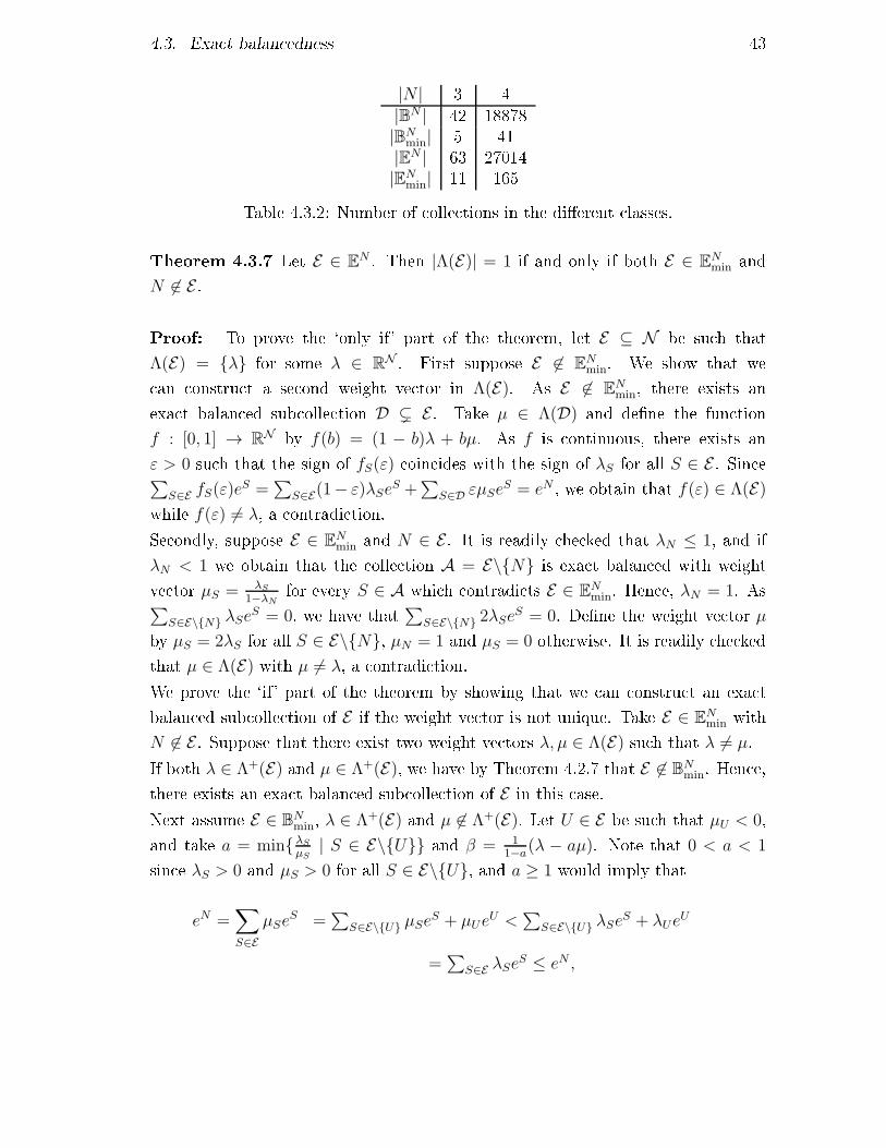
4.3. Exa t balan edness 43|N | 3 4|BN | 42 18878|BN

min| 5 41|EN | 63 27014|EN

min| 11 165Table 4.3.2: Number of olle tions in the di�erent lasses.Theorem 4.3.7 Let E ∈ EN . Then |Λ(E)| = 1 if and only if both E ∈ ENmin and

N 6∈ E .Proof: To prove the `only if' part of the theorem, let E ⊆ N be su h thatΛ(E) = {λ} for some λ ∈ RN . First suppose E 6∈ EN

min. We show that we an onstru t a se ond weight ve tor in Λ(E). As E 6∈ ENmin, there exists anexa t balan ed sub olle tion D ( E . Take µ ∈ Λ(D) and de�ne the fun tion

f : [0, 1] → RN by f(b) = (1 − b)λ + bµ. As f is ontinuous, there exists anε > 0 su h that the sign of fS(ε) oin ides with the sign of λS for all S ∈ E . Sin e∑

S∈E fS(ε)eS =

∑S∈E(1− ε)λSe

S +∑

S∈D εµSeS = eN , we obtain that f(ε) ∈ Λ(E)while f(ε) 6= λ, a ontradi tion.Se ondly, suppose E ∈ EN

min and N ∈ E . It is readily he ked that λN ≤ 1, and ifλN < 1 we obtain that the olle tion A = E\{N} is exa t balan ed with weightve tor µS = λS

1−λNfor every S ∈ A whi h ontradi ts E ∈ EN

min. Hen e, λN = 1. As∑S∈E\{N} λSe

S = 0, we have that ∑S∈E\{N} 2λSeS = 0. De�ne the weight ve tor µby µS = 2λS for all S ∈ E\{N}, µN = 1 and µS = 0 otherwise. It is readily he kedthat µ ∈ Λ(E) with µ 6= λ, a ontradi tion.We prove the `if' part of the theorem by showing that we an onstru t an exa tbalan ed sub olle tion of E if the weight ve tor is not unique. Take E ∈ EN

min withN 6∈ E . Suppose that there exist two weight ve tors λ, µ ∈ Λ(E) su h that λ 6= µ.If both λ ∈ Λ+(E) and µ ∈ Λ+(E), we have by Theorem 4.2.7 that E 6∈ BN

min. Hen e,there exists an exa t balan ed sub olle tion of E in this ase.Next assume E ∈ BNmin, λ ∈ Λ+(E) and µ 6∈ Λ+(E). Let U ∈ E be su h that µU < 0,and take a = min{λS

µS| S ∈ E\{U}} and β = 1

1−a(λ − aµ). Note that 0 < a < 1sin e λS > 0 and µS > 0 for all S ∈ E\{U}, and a ≥ 1 would imply that

eN =∑

S∈E

µSeS =

∑S∈E\{U} µSe

S + µUeU <

∑S∈E\{U} λSe

S + λUeU

=∑

S∈E λSeS ≤ eN ,

44 Chapter 4. Minimal exa t balan ednesswhere the stri t inequality uses that µU < 0 < λU . Note that βS = 11−a

(λS−aµS) ≥ 0for all S ∈ E , with equality for at least one oalition. If we take B = {S ∈

E | βS > 0}, then B is a proper subset of E and ∑S∈B βSeS =

∑S∈E βSe

S =∑S∈E

(λS

1−aeS − aµS

1−aeS)= eN , so B ∈ BN whi h ontradi ts E ∈ BN

min.Finally, let λ 6∈ Λ+(E) and µ 6∈ Λ+(E). This means that there exist oalitions T ∈ Eand U ∈ E su h that λT < 0 and µU < 0.Assume T = U . Take a = min{λS

µS| S ∈ E}. Note that a > 0 sin e for S ∈ Eeither both λS > 0 and µS > 0 or both λS < 0 and µS < 0. It holds that a < 1,as a ≥ 1 would imply that either λ = µ or ∑S∋i λS >

∑S∋i µS = 1 for i ∈ N\T ,a non-empty set sin e by assumption N 6∈ E . We onstru t δ = 1

1−aλ − a

1−aµ and

D = {S ∈ E | δS 6= 0}. It is readily veri�ed that δS ≥ 0 for all S ∈ D\{T} and∑S∈D δSe

S = eN . This shows that D ∈ EN and by onstru tion D ( E , whi h ontradi ts E ∈ ENmin.Now assume T 6= U . Take a = µT

µT−λT. It is readily he ked that 0 < a < 1. Take

δ = aλ+(1−a)µ and D = {S ∈ E | δS 6= 0}. We have δS > 0 for every S ∈ D\{T, U}and δT = 0. Sin e ∑S∈D δSeS =

∑S∈E aλSe

S +∑

S∈E(1 − a)µSeS = eN this showsthat D ∈ EN whi h ontradi ts E ∈ EN

min. �As Example 4.3.8 shows, there exist minimal exa t balan ed olle tions with morethan one exa t balan ed weight ve tor. By Theorem 4.3.7 su h a olle tion must ontain the set N .Example 4.3.8 Take N = {1, 2, 3}. The olle tion E = {{1}, {2}, {1, 2}, N} isminimal exa t balan ed, but there exists more than one weight ve tor: de�ne λ byλ{1} = λ{2} = 1, λ{1,2} = −1 and λN = 1 and µ by µ{1} = µ{2} = 2, µ{1,2} = −2 andµN = 1. It is readily he ked that λ ∈ Λ(E) and µ ∈ Λ(E). ⊳If a minimal exa t balan ed olle tion does ontain the grand oalition, then thereexists more than one exa t balan ed weight ve tor, but these weight ve tors arerelated in a spe ial way and indu e the same onstraint on the game. Furthermore,if for an exa t balan ed olle tion all weight ve tors indu e the same onstraint onthe game, then the olle tion is minimal exa t balan ed.Theorem 4.3.9 Let E ∈ EN . Then both E ∈ EN

min and N ∈ E if and only if forevery λ ∈ Λ(E) and µ ∈ Λ(E) there exists a s alar a > 0 su h that

4.3. Exa t balan edness 45µS = aλS for all S ∈ E\{N},

µN = λN = 1.Proof: For the `only if' part of the proof, assume E ∈ ENmin and N ∈ E . Let

λ ∈ Λ(E). It is readily he ked that λN ≤ 1, and if λN < 1 we obtain that the olle tion C = E\{N} is exa t balan ed with weight ve tor γS = λS

1−λNfor every

S ∈ C and γS = 0 otherwise. Hen e, λN = 1.Take T ∈ E su h that λT < 0. Su h a T ∈ E exists, as N ∈ E and thereforeE 6∈ BN

min. As ∑S∈E\{N} λSeS = 0 and λS > 0 for all S ∈ E\{T}, we obtainthat S ( T for all S ∈ E\{T,N}. This implies that the lo ation of the negativeweight is unique, µT < 0 for every µ ∈ Λ(E). Rewriting ∑S∈E\{N} λSe

S = 0 yields∑S∈E\{N,T}−

λS

λTeS = eT , and therefore E\{N, T} ∈ BT . If there exists a minimalbalan ed olle tion B ∈ BT

min su h that B ( E\{T,N}, it is readily he ked thatB ∪ {T,N} is an exa t balan ed olle tion, whi h ontradi ts our assumption ofE ∈ EN

min. Hen e, E\{N, T} ∈ BTmin. Sin e E\{N, T} ∈ BT

min, by Theorem 4.2.7 thereis a unique balan ed ve tor of weights β of E\{N, T}. Note thateN = eN + λT e

T +∑

S∈E\{N,T}

λSeS

= eN + λT∑

S∈E\{N,T}

βSeS +

∑

S∈E\{N,T}

λSeS

= eN +∑

S∈E\{N,T}

(λTβS + λS)eS.This implies that ∑S∈E\{N,T}(λTβS + λS)e

S = 0. If λTβS 6= λS for some S ∈

E\{N, T} we have γ ∈ BTmin where we de�ne for small ε > 0, γS = βS+ε(λTβS+λS)for every S ∈ E\{N, T} and γS = 0 otherwise. So, λTβS + λS = 0 and therefore

λS = −λTβS for every S ∈ E\{N, T}. Now take µ ∈ Λ(E) and take a = µT

λT. Sin e

µT < 0 and λT < 0, a > 0. We have µT = aλT by de�nition, and µS = −µTβS =

−aλTβS = λS for every S ∈ E\{N, T}.For the `if' part of the proof, assume that for every λ ∈ Λ(E) and µ ∈ Λ(E),λN = µN = 1 and there exists an a > 0 su h that µS = aλS for every S ∈ E\{N}.Clearly we have N ∈ E . Suppose E 6∈ EN

min. As E is not minimal, there exists aD ( E su h that D ∈ EN

min. Let λ ∈ Λ(E) and δ ∈ Λ(D). De�ne µ = (1− b)λ + bδ,where b > 0 is su� iently small, su h that the sign of δS equals the sign of µS forevery S ∈ E . Clearly, µ ∈ Λ(E). Take T ∈ E\D and U ∈ D, U 6= N . Su h a

46 Chapter 4. Minimal exa t balan ednessU exists, as {N} is not a minimal exa t balan ed olle tion by de�nition. Sin eµT = (1− b)λT and µU = (1− b)λU + bδU 6= (1− b)λU , there does not exist a s alara > 0 su h that µT = aλT and µU = aλU , whi h is a ontradi tion. Hen e, E ∈ EN

min.As we showed before that N ∈ E , this ompletes the proof. �For minimal balan ed olle tions, the orresponding weight ve tor is unique. Sim-ilarly, we have shown that for minimal exa t balan ed olle tions either the or-responding weight ve tor is unique or all orresponding weight ve tors indu e thesame onstraint on the game. This way, for every minimal exa t balan ed olle tionwe an use one standardized weight ve tor . In the remainder, for every minimalbalan ed olle tion B we denote βB for the unique balan ed weight ve tor. Moregeneral, for every E ∈ ENmin with N 6∈ E , we denote λE for the unique exa t balan- ed weight ve tor. For E ∈ EN

min with N ∈ E , λE denotes the standardized exa tbalan ed weight ve tor su h that min{λES | S ∈ E} = −1. Noti e that for notational onvenien e, for B ∈ BNmin the standardized weight ve tor is both denoted by βB and

λB.4.4 Partitioning the lass of minimal exa t balan ed olle tionsIn this se tion we study the stru ture of the lass of minimal exa t balan ed ol-le tions. It turns out that this set an be de omposed in three parts, all related tobalan ed olle tions. The �rst part onsists of all minimal balan ed olle tions.Theorem 4.4.1 BNmin ⊆ EN

min.Proof: Let B ∈ BNmin. It is lear that every minimal balan ed olle tion is alsoexa t balan ed. It remains to show that it is also minimal exa t balan ed. Assumethere exists an exa t balan ed olle tion E ( B and take λ ∈ Λ(E). We will showthat this results in a ontradi tion with B ∈ BN

min.Sin e B ∈ BNmin we know that there exists a T ∈ E su h that λT < 0 as B doesnot have a proper subset that is balan ed. Take a = min{

βBS

λS| S ∈ E\{T}} and

γ = 11−a

(βB − aλ). Note that 0 < a < 1 sin e βBS > 0 and λS > 0 for all S ∈ E\{T},and a ≥ 1 would imply that

4.4. Partitioning the lass of minimal exa t balan ed olle tions 47∑

S∈E

λSeS =

∑

S∈E\{T}

λSeS + λT e

T ,

<∑

S∈E\{T}

βBS e

S + βBT e

T ,

=∑

S∈E

βBS e

S,

≤ eN .Now γS ≥ 0 for all S ∈ B, with equality for at least one oalition. De�ne the olle tion C = {S ∈ E | γS > 0}. Then C is a proper subset of B and∑

S∈C

γSeS =

∑

S∈B

γSeS =

∑

S∈B

βBS

1− aeS −

∑

S∈E

aλS1− a

eS =1

1− aeN −

a

1− aeN = eN ,so C ∈ BN , ontradi ting B ∈ BN

min. �The se ond part of the partition of ENmin onsists of so- alled negative balan ed olle -tions. The set of all negative balan ed olle tions is denoted by B

N

min. The negativebalan ed olle tions an be obtained, by repla ing one oalition in a minimal balan- ed olle tion by its omplement. However, this is only allowed for the oalitionswith weight stri tly smaller than 1. We haveBN

min = {(B\{S}) ∪ {N\S} | B ∈ BNmin, S ∈ B : βB

S < 1}.Example 4.4.2 Let N = {1, 2, 3, 4}, and onsider the minimal balan ed olle tionB = {{1, 2}, {1, 3}, {2, 3}, {4}}. For the weight ve tor βB it holds that βB

{1,2} = 12.This means that E = (B\{{1, 2}})∪ ({{3, 4}}) = {{3, 4}, {1, 3}, {2, 3}, {4}} ∈ B

N

min.It is readily he ked that E ∈ EN , sin e e{1,3}+e{2,3}+2e{4}−e{3,4} = eN . As βB{4} = 1,we annot repla e the oalition {4} by its omplement to obtain an element of BN

min.⊳The exa t balan ed weight ve tor of a negative balan ed olle tion an be derivedfrom the balan ed weight ve tor of the orresponding balan ed olle tion.Theorem 4.4.3 Let E ∈ B

N

min. Let B ∈ BNmin and U ∈ B be su h that E =

(B\{U}) ∪ {N\U} and βBU < 1. Let λS =

βBS

1−βBU

for all S ∈ B\{U}, λN\U = −βBU

1−βBUand λS = 0 for S ∈ N\E . Then λ ∈ Λ(E).

48 Chapter 4. Minimal exa t balan ednessProof: As B ∈ BNmin and βB

U < 1, we know N\U 6∈ B. As 0 < βBU < 1, we obtainthat λS =

βBS

1−βBU

> 0 for all S ∈ E\{U} and λN\U = −βBU

1−βBU

< 0. For i ∈ U ,∑

S∈E,

S∋i

λS =∑

S∈(B\{U})∪{N\U},

S∋i

λS =∑

S∈(B\{U}),

S∋i

βBS

1− βBU

=1

1− βBU

∑

S∈B\{U},

S∋i

βBS = 1,and for i ∈ N\U it holds that

∑

S∈E,S∋i

λS =∑

S∈(B\{U})∪{N\U},

S∋i

λS =∑

S∈B,

S∋i

βBS

1− βBU

−βBU

1− βBU

=1

1− βBU

∑

S∈B,

S∋i

βBS − βB

U

= 1.So, indeed λ ∈ Λ(E). �By de�nition of BN

min and the observation that N 6∈ B for every B ∈ BNmin, we have

N 6∈ E for every E ∈ BN

min. Hen e, for this se ond part of the partition we an fo uson olle tions without the grand oalition. Consider su h a olle tion whi h is notminimal balan ed. Then it is minimal exa t balan ed if and only if it is negativebalan ed.Theorem 4.4.4(i) BN

min ⊆ ENmin\B

Nmin.(ii) Let E ∈ EN

min\BNmin and N 6∈ E . Then E ∈ B

N

min.Proof:(i) Let E ∈ BN

min. Let B ∈ BNmin and U ∈ B be su h that E = (B\{U})∪ {N\U} and

βBU < 1. Let λS =

βBS

1−βBU

for all S ∈ B\{U}, λN\U = −βBU

1−βBU

and λS = 0 for S ∈ N\E .From Theorem 4.4.3, it follows that λ ∈ Λ(E) and therefore E ∈ EN .We prove that E ∈ ENmin. Assume on the ontrary that there exists a subset D ( E ,with D ∈ EN

min. By minimality of B, it must hold that N\U ∈ D as otherwise D ( Bwhi h would ontradi t Theorem 4.4.1.We distinguish two ases:(1) Assume λDS > 0 for all S ∈ D\{N\U}. We know λDN\U < 1, sin e λDN\U = 1would mean that D\{N\U} is a balan ed olle tion on U whi h ontradi tsminimality of B as we an omit U from B. Given that λDN\U < 1, we an

4.4. Partitioning the lass of minimal exa t balan ed olle tions 49reverse the pro edure for onstru ting E : take A = (D\{N\U}) ∪ ({U}) andtake αS =λDS

1−λDN\U

for all S ∈ D\{N\U} and αU = −λDN\U

1−λDN\U

. We obtain αS > 0for all S ∈ A\{U} and αU 6= 0. Furthermore, for i ∈ U :∑

S∈A,S∋i

αS = −λDN\{U}

1− λDN\U

+∑

S∈D\{N\U},S∋i

λDS1− λDN\U

= 1,and for i ∈ N\U it holds that∑

S∈A,S∋i

αS =∑

S∈D\{N\U},S∋i

λDS1− λDN\U

= 1,So, α ∈ Λ(A) and therefore A ∈ EN . As A ( B this ontradi ts our assump-tion of B ∈ ENmin.(2) Assume λDT < 0 for some T ∈ D\{N\U}, whi h means that D ∈ EN

min\BNminand λDN\U > 0. Take c = −

λDN\U

λEN\U

, and take T ∈ D su h that λDT < 0. We onstru t the weight ve tor γ with γS = c1+c

λES + 11+c

λDS for all S ∈ E andγS = 0 if S ∈ N\E . Furthermore, take C = {S ∈ E | γS 6= 0}. By de�nition ofγ, we obtain γN\U = 0 and γS > 0 for all S ∈ C\{T}. So, C ( B and γ ∈ Λ(C).Therefore B 6∈ EN

min, a ontradi tion with Theorem 4.4.1.So, we have E ∈ ENmin. From Theorem 4.3.7 it follows that Λ(E) = {λ}. Sin e λN\U ,

E ∈ ENmin\B

Nmin.(ii) Let E ∈ EN

min\BNmin and N 6∈ E . We will identify B ∈ BN

min and the oalitionT ∈ B su h that βB

T < 1 and E = (B\{T}) ∪ {N\T}. Take T ∈ E su h thatλET < 0. Take B = (E\{T}) ∪ {N\T} and de�ne βS =

λES

1−λET

for all S ∈ E\{T} andβN\T = −

λET

1−λET

. We obtain βS > 0 for all S ∈ B. Furthermore, for i ∈ N\T :∑

S∈B,S∋i

βS = −λET

1− λET−

∑

S∈E,S∋i

λES1− λET

= 1,

50 Chapter 4. Minimal exa t balan ednessand for i ∈ T it holds that∑

S∈B,S∋i

βS =∑

S∈E\{T},S∋i

λES1− λET

= 1,So, B ∈ BN . It remains to show that B is minimal. Here we need the onditionthat N 6∈ E , sin e there is no minimal balan ed olle tion that ontains N . If B isnot minimal, then there exists a B′ ∈ BNmin su h that B′ ( B. More pre isely, asevery balan ed olle tion is the union of minimal balan ed olle tions there exists a

B′ ∈ BNmin su h that B′ ( B and N\T ∈ B′.First suppose there exists a B′ ( B withN\T ∈ B′ and β ′ ∈ Λ+(B′) su h that β ′

N\T <

1. Take su h a B′. Then we obtain by de�nition of BN

min that (B′\{N\T})∪ ({T}) ∈

BN

min ⊆ ENmin\B

Nmin. Consequently, we have B′\{N\T}∪{T} ( E , a ontra tion withthe minimality of E .Next suppose that for every minimal balan ed olle tion C ( B with N\T ∈ C itholds that βC

N\T = 1. Take su h a minimal balan ed olle tion C ( B with N\T ∈ C.We de�ne a new olle tion D = C\{N\T}. Sin e N\T 6∈ D, we have D ( E . Also,∑S∈B β

CSe

S = eN and therefore ∑S∈D βCSe

S = eN − βCN\T e

N\T = eT . Take δS = βCSfor every S ∈ D and δT = −1, and we have (1 − a)λE + aδ ∈ Λ(E) for a ∈ (0, 1).This ontradi ts the minimality of E , sin e by Theorem 4.3.7 |Λ(E)| = 1.Hen e, B ∈ BN

min, E = B\{N\T} ∪ {T} and βBN\T < 1, so E ∈ B

N

min. �By de�nition, the grand oalition is not ontained in any negative balan ed olle -tion. Hen e, by Theorem 4.4.4 and 4.3.7, for every negative balan ed olle tion theexa t balan ed weight ve tor is unique. Let E ∈ BN

min, take B ∈ BNmin and U ∈ Bsu h that E = (B\{U}) ∪ {N\U}. By Theorem 4.4.3, the negative weight is pla edon N\U . Sin e the exa t balan ed weight ve tor is unique, this implies that forevery E ∈ B

N

min there is a unique olle tion B ∈ BNmin and a unique oalition U ∈ Bsu h that E = (B\{U}) ∪ {N\U}.The third part of the partition onsists of the minimal subbalan ed olle tions.These olle tions onsist of all minimal balan ed olle tions of the proper subsets ofthe player set with at least two players, to whi h the oalition formed by all playersof the subset and the oalition formed by all players of the original player set areadded.For every M ( N su h that |M | ≥ 2, de�ne

BNmin(M) = {B ∪ {M,N} | B ∈ BM

min},

4.4. Partitioning the lass of minimal exa t balan ed olle tions 51Also, de�neBNmin = ∪M(N,|M |≥2BN

min(M),as the set of all minimal subbalan ed olle tions.Theorem 4.4.5 Let E ∈ BNmin. Let M ( N and B ∈ BM

min be su h that E =

(B ∪ {M,N}). Let λS = βBS for all S ∈ B, λM = −1, λN = 1 and λS = 0 for all

S ∈ N\E . Then λ ∈ Λ(E).Proof: It is readily he ked that ∑S∈E λSeS =

∑S∈B β

BS e

S − eM + eN = eN andλS > 0 for all S ∈ E\{M}. Hen e, λ ∈ Λ(E). �Theorem 4.4.6(i) BN

min ⊆ ENmin\B

Nmin,(ii) Let E ∈ EN

min\BNmin and N ∈ E . Then E ∈ BN

min.Proof:(i) Let E ∈ BNmin. Let M ( N and B ∈ BM

min be su h that E = (B\{M,N}). LetλS = βB

S for all S ∈ B, λM = −1, λN = 1 and λS = 0 for all S ∈ N\E . Theorem4.4.5 shows that λ ∈ Λ(E), so E ∈ EN .Suppose E 6∈ ENmin. Take D ( E su h that D ∈ EN

min. We have N ∈ D sin ethe players in N\M are not present in any other oalition in E . This also impliesthat λDN = 1. As {N} 6∈ EN we have ∑S∈D\{N} λDS = 0. This means that thereexists a T ∈ D\{N} su h that λDT < 0 and S ⊆ T for all S ∈ D\{N}. We obtain

D\{N, T} ∈ BT .First, suppose T = M . Then D ( E gives D\{N,M} ( B whi h ontradi tsB ∈ BM

min.Se ond, suppose T 6=M . As M 6∈ D, D\{N} ( B. De�ne the weight ve tor δ su hthat δS = λDS for all S ∈ D\{N} and δS = 0 otherwise. Now, for small ε > 0 wehave ελD + βB ∈ Λ+(B) whi h ontradi ts B ∈ BMmin by Theorem 4.2.7.(ii) By Theorem 4.3.9 we have λEN = 1. Take T ∈ E su h that λET = −1.

52 Chapter 4. Minimal exa t balan edness|N | 3 4 5

|ENmin| 11 165 8572

|BNmin| 5 41 1474

|BN

min| 3 98 6833|BN

min| 3 26 265Table 4.4.1: Number of olle tions in the three parts of the partitionWe have ∑S∈E\{N} λSeS = 0 whi h yields ∑S∈E\{N,T} λSe

S = eT , and thereforeE\{N, T} ∈ BT . If there exists a minimal balan ed olle tion B ∈ BT

min su h thatB ( E\{T,N}, it is readily he ked that B ∪ {T,N} is an exa t balan ed olle -tion, whi h ontradi ts our assumption of E ∈ EN

min. Hen e, E\{N, T} ∈ BTmin and

E ∈ BNmin. �So, we established that BN

min, BN

min, and BNmin are ontained in EN

min. By de�nition,N 6∈ E for every E ∈ B

N

min and N ∈ E for every E ∈ BNmin. For E ∈ EN

min\BNmin, if

N 6∈ E then E ∈ BN

min, and if N ∈ E then E ∈ BNmin. Hen e, we obtain the following orollary from Theorem 4.4.1, Theorem 4.4.4 and Theorem 4.4.6.Corollary 4.4.7 The three sets BN

min, BN

min, and BNmin form a partition of EN

min.The number of olle tions in the di�erent parts of the partition are shown in Ta-ble 4.4.1. Appendix 4.A ontains the minimal balan ed, minimal subbalan ed andminimal negative balan ed olle tions for three and four players. To generate these olle tions we used the results by Peleg (1965), whi h provides an e� ient and om-prehensive algorithm for obtaining all minimal balan ed olle tions. As we derivedan expli it relation between minimal balan ed olle tions on the one hand and mini-mal negative balan ed olle tions and minimal subbalan ed olle tions on the otherhand ( f. Theorem 4.4.4 and Theorem 4.4.6), these olle tions an be onstru tedfrom the minimal balan ed olle tions together with their respe tive weight ve tors( f. Theorem 4.4.3 and Theorem 4.4.5).4.5 Su� ient onditions for exa tnessAs mentioned before, the lass of minimal balan ed olle tions is useful as one doesnot need other balan ed olle tions to he k whether a game is balan ed. The lassof minimal exa t balan ed weights exhibits the same feature: we show that we only

4.5. Su� ient onditions for exa tness 53need the minimal exa t balan ed olle tions to he k whether a game is exa t. Toprove this, we �rst need the following lemma.Lemma 4.5.1 Let U ∈ N , A ⊆ {S ∈ N | S ( U} and α ∈ RN+ su h that∑

S∈A αSeS = eU , αS > 0 for every S ∈ A and αS = 0 for every S ∈ 2U\(A∪{U}).Let v ∈ ∩E∈BN

min(U)V (E). Then ∑S∈A αSv(S) ≤ v(U).Proof: Take (U, vU) su h that vU(S) = v(S) for every S ∈ 2U , and take αU ∈ R2Usu h that αUS = αS for every S ∈ 2U . Sin e∑S∈A α

US e

S = eU , we have A ∈ BU withαU the orresponding balan ed weight ve tor. By Theorem 4.2.6, this means thatthere exist A1, ...,Am ∈ BU

min with balan ed weight ve tors α1, ..., αm ∈ R2U su hthat if∑

S∈Ai

αiSv

U(S) ≤ vU(U) for every i ∈ {1, ..., m},then∑

S∈A

αUS v

U(S) ≤ vU(U).Note that ∑S∈A αUS v

U(S) ≤ vU(U) dire tly implies ∑S∈A αSv(S) ≤ v(U). Weshow that for every i ∈ {1, ..., m}, ∑S∈AiαiSv

U(S) ≤ vU(U) follows from v ∈

∩E∈BNmin(U)V (E).Take i ∈ {1, ..., m} and Ci = Ai ∪ {U,N}. By de�nition, we have Ci ∈ BN

min(U) withλCiS = αi

S for every S ∈ Ci, λCiU = −1 and λCiN = 1. We obtain∑

S∈Ai

αiSv

U(S) =∑

S∈Ai

αiSv(S)

=∑

S∈Ci

λCiS v(S) + v(U)− v(N)

≤ v(N) + v(U)− v(N)

= vU(U),where the inequality follows from v ∈ ∩E∈BNmin(U)V (E). Hen e, for every i ∈

{1, ..., m}, ∑S∈AiαiSv

U(S) ≤ vU(U) and therefore ∑S∈A αSv(S) ≤ v(U). �Theorem 4.5.2 Let v ∈ V (E) for all E ∈ ENmin. Then v ∈ V .

54 Chapter 4. Minimal exa t balan ednessProof: In fa t, we prove the following statement. Let D ∈ EN\ENmin, and assume

∩E∈ENminV (E) ⊆ V (A) for every A ( D. Then ∩E∈EN

minV (E) ⊆ V (D). Clearly, thisholds for every D ∈ EN\EN

min with |D| = 0. By indu tion on |D| we then obtain∩E∈EN

minV (E) = ∩E∈ENV (E) = V .To show that ∩E∈EN

minV (E) ⊆ V (D), we show ∩E∈EN

minV (E) ⊆ V (δ) for every δ ∈

Λ(D). Let δ ∈ Λ(D).First, assume δ ∈ Λ+(D). Then Theorem 4.4.1 and Theorem 4.2.6 imply thatv ∈ V (δ).Se ond, assume that δ 6∈ Λ+(D). Take U ∈ D su h that δU < 0.If U = N , then de�ne C = D\{N} and γS = δS

1−δNfor all S ∈ C and γS = 0 for all

S ∈ N\C. We have γ ∈ Λ+(C) and C ∈ BN . Note that v ∈ V (δ) is dire tly impliedby v ∈ V (γ). Hen e, in the remainder we will assume that U 6= N .Sin e D 6∈ ENmin, we an take A ∈ EN

min su h that A ( D.If A ∈ ENmin\B

Nmin, then take T ∈ A su h that λAT < 0. If A ∈ BN

min, de�ne T = ∅.De�ne a = min{ δSλAS

| S ∈ A\{T, U}}. We �rst show that a ≤ 1.Suppose on the ontrary that a > 1. As δS > λAS for every S ∈ D\{U}, we have fori ∈ N\U that

∑

S∈D,

S∋i

δS =∑

S∈D\{U},

S∋i

δS >∑

S∈D\{U},

S∋i

λAS = 1,a ontradi tion.We dis riminate between two ases:• a = 1. If T\U 6= ∅, then for i ∈ T\U it holds that

∑

S∈D,

S∋i

δS =∑

S∈D\{T,U},

S∋i

δS + δT >∑

S∈D\{T,U},

S∋i

λAS + λAT = 1,whi h annot hold. So, T\U = ∅. If δU = λAU then δR > λAR for some R ∈ Awould give∑

S∈D,

S∋i

δS >∑

S∈D,

S∋i

λAS = 1,

4.5. Su� ient onditions for exa tness 55for i ∈ R. Hen e, δS = λS for every S ∈ D but this ontradi ts A ( D.So, we on lude T\U = ∅ and δU < λAU , implying λAU − δU > 0. De�neκS =

δS−λAS

λAU−δU

for all S ∈ D\{U}, and κS = 0 for all S ∈ N\(D\{U}). TakeK = {S ∈ D\{U} | κS 6= 0}. Note that κS > 0 for all S ∈ K and

∑

S∈K

κSeS =

1

λAU − δU

∑

S∈D\{U}

(δS − λAS )eS

=1

λAU − δU

∑

S∈D\{U}

δSeS −

∑

S∈A\{U}

λAS eS

=1

λAU − δU(eN − δUe

U − eN + λAUeU)

= eU .Hen e, K ⊆ {S ∈ N | S ( U}, ∑S∈K κSeS = eU , κS > 0 for every S ∈ A and

κS = 0 for every S ∈ 2U\(K∪{U}). So, we an apply Lemma 4.5.1. Therefore∑

S∈D

δSv(S) = (λAU − δU)∑

S∈D

δS − λASλAU − δU

v(S)

+∑

S∈D

λASv(S)

= (λAU − δU)

(∑

S∈K

κSv(S)− v(U)

)

+∑

S∈A

λASv(S)

≤ (λAU − δU)(v(U)− v(U)) + v(N)

= v(N),where the inequality follows from Lemma 4.5.1 and v ∈ V (λA). Hen e,(∩E∈BN

min(U)V (E))∩V (A) ⊆ V (δ). Sin e BNmin(U) ⊆ EN

min and A ∈ ENmin, we annow on lude that ∩E∈EN

minV (E) ⊆ V (δ).

56 Chapter 4. Minimal exa t balan edness• a < 1. We de�ne κS = 1

1−aδS −

a1−a

λAS for all S ∈ D, κS = 0 for S ∈ N\D andde�ne K = {S ∈ D | κS 6= 0}. By de�nition of a, K ( D. Note that K ∈ ENand κ ∈ Λ(K), as κS > 0 for all S ∈ K\{U}, κU < 0, and∑

S∈K

κSeS =

∑

S∈D

(1

1− aδS −

a

1− aλAS )e

S

=1

1− a

∑

S∈D

δSeS −

a

1− a

∑

S∈A

λAS eS

= eN .It is now easily seen that V (κ) ∩ V (λA) ⊆ V (δ), as∑

S∈D

δSv(S) = (1− a)∑

S∈K

κSv(S) + a∑

S∈A

λAS v(S) ≤ v(N).Hen e, V (K) ∩ V (A) ⊆ V (δ). Sin e K ⊆ D and A ∈ ENmin, by indu tion we an now on lude that ∩E∈EN

minV (E) ⊆ V (δ).

�As Theorem 4.2.8 states, the set of balan ed games an not be hara terized by asubset of the minimal balan ed olle tions. However, the set of exa t games anbe hara terized by a subset of the minimal exa t balan ed olle tions, as thereexist minimal exa t balan ed olle tions that are redundant. The following exampleillustrates this.Example 4.5.3 Consider the minimal exa t balan ed olle tions B =

{{1, 2}, {1, 3}, {2, 3}} with weight ve tor βB su h that βB{1,2} = βB

{1,3} = βB{2,3} = 1

2,

C = {{1}, {2, 3}} with weights βC{1} = βC

{2,3} = 1 and E = {{1, 2}, {1, 3}, {1}}with λE{1,2} = λE{1,3} = 1 and λE{1} = −1. We have V (C) ∩ V (E) ⊆ V (B), sin eβB = 1

2βC + 1

2λE . ⊳The question arises whi h minimal exa t balan ed olle tions we an dis ard. Itturns out that for |N | ≥ 3, ∩E∈EN

min\BNminV (E) ⊆ V . So, we an omit all the minimalbalan ed onditions. To show this, we �rst introdu e a lemma to onstru t parti ularmembers of EN

min.

4.5. Su� ient onditions for exa tness 57Lemma 4.5.4 Let |N | ≥ 3 and take S ∈ N and T ∈ N su h that S ∩ T = ∅.(i) If S ∪ T = N , |T | ≥ 2 and i ∈ T , then {S ∪ {i}, T, {i}} ∈ ENmin\B

Nmin.(ii) If S ∪ T 6= N , then {S, T, S ∪ T,N} ∈ EN

min\BNmin.Proof:(i) The olle tion {S∪{i}, T, N\{i}} is minimal balan ed with weight ve tor λ su hthat λS∪{i} = λT = λN\{i} = 1

2. By de�nition of BN

min, we have {S ∪ {i}, T, {i}} ∈

BN

min. By Theorem 4.4.4 this means that {S ∪ {i}, T, {i}} ∈ ENmin\B

Nmin.(ii) The olle tion {S, T} is minimal balan ed for player set S ∪ T . By de�ni-tion of BN

min(S ∪T ), we have {S, T, S ∪ T,N} ∈ BNmin(S ∪ T ). By Theorem 4.4.6 thismeans that {S, T, S ∪ T,N} ∈ EN

min\BNmin. �Theorem 4.5.5 Let v ∈ V (E) for every E ∈ EN

min\BNmin and |N | ≥ 3. Then v ∈ V .Proof: Let B ∈ BN

min. We show that ∩E∈ENmin\B

NminV (E) ⊆ V (B). First, onsider the ase where B is a partition.Assume B = {S, T} for some S, T ∈ N . Note that βB

S = βBT = 1. Without lossof generality, we assume |S| ≤ |T |. Take i ∈ T , A = {{i}, S, S ∪ {i}, N} with

λA{i} = λAS = λAN = 1 and λAS∪{i} = −1 and D = {S ∪ {i}, T, {i}} with λDS∪{i} =

λDT = 1 and λD{i} = −1. By Lemma 4.5.4, A ∈ ENmin\B

Nmin and D ∈ EN

min\BNmin. Now

V (A) ∩ V (D) ⊆ V (B) as∑

U∈B

βBUv(U) = v(S) + v(T )

= (v({i}) + v(S)− v(S ∪ {i}) + v(N))

+ (v(S ∪ {i}) + v(T )− v({i}))

− v(N)

=∑

U∈A

λAUv(U) +∑

U∈D

λDUv(U)− v(N)

≤ v(N),where the inequality follows from v ∈ V (A) and v ∈ V (D).

58 Chapter 4. Minimal exa t balan ednessWe show that for every partition B with |B| ≥ 3 there exists a partition C su hthat |C| < |B| and ∩E∈ENmin\B

NminV (E) ∩ V (C) ⊆ V (B). This su� es to show that

∩E∈ENmin\B

NminV (E) ⊆ V (B) for every partition B ∈ BN

min.Assume that B is a partition of the player setN , with |B| ≥ 3. Take S ∈ B and T ∈ Bwith S 6= T . De�ne A = {S, T, S ∪ T,N} with λAS = λAT = λAN = 1 and λAS∪T = −1.By Lemma 4.5.4 we have A ∈ ENmin\B

Nmin. De�ne D = (B\{S, T}) ∪ {S ∪ T} and

δ ∈ Λ(D) su h that δS = 1 for all S ∈ D. Note that D is a partition and |D| < |B|.Now V (A) ∩ V (D) ⊆ V (B) as∑

U∈B

βBUv(U) =

∑

U∈B\{S,T}

βBUv(U) + v(S) + v(T )

=∑

U∈B\{S,T}

βBUv(U) + v(S ∪ T )

+ v(S) + v(T )− v(S ∪ T ) + v(N)

− v(N)

=∑

U∈D

λDUv(U) +∑

U∈A

λAUv(U)− v(N)

≤ v(N),where the inequality follows from v ∈ V (A) and v ∈ V (D).Se ond, onsider the ase where B is not a partition. Take T ∈ B su h that βBT < 1.As B is not a partition, su h a oalition exists and N\T 6∈ B. De�ne C = {T,N\T}and D = (B\{T}) ∪ {N\T} with δS =

βBS

1−βBT

for all S ∈ B\{T} and δN\T = −βBT

1−βBT

.We have already shown that ∩E∈ENmin\B

NminV (E) ⊆ V (C). Furthermore, by Theorem4.4.4 we know that D ∈ EN

min\BNmin. Now V (C) ∩ V (D) ⊆ V (B) as

∑

S∈B

βBS v(S) =

∑

S∈B\{T}

βBSv(S) + βB

T v(T )

= (1− βBT )

∑

S∈B\{T}

βBS

1− βBT

v(S)−βBT

1− βBT

v(N\T )

+ βBT (v(T ) + v(N\T ))

= (1− βBT )∑

S∈D

δSv(S) + βT∑

S∈C

βCSv(S)

≤ v(N),where the inequality follows from v ∈ V (C) and v ∈ V (D). So ∩E∈ENmin\B

NminV (E) ⊆

∩B∈BNminV (B).

4.5. Su� ient onditions for exa tness 59Therefore, ∩E∈ENmin\B

NminV (E) = ∩E∈EN

minV (E) = ∩E∈ENV (E) = V . So, v ∈ V if andonly if v ∈ v(E) for all E ∈ EN

min\BNmin. �We have shown that the lass of minimal balan ed olle tions is redundant to verifythat a game is exa t. However, as the following example demonstrates, there existsan even smaller sub lass of the lass of minimal exa t balan ed olle tions that stillensures exa tness of the game.Example 4.5.6 Let N = {1, 2, 3, 4}. Consider the minimal exa t balan ed ol-le tions A = {{2}, {1, 4}, {1, 2, 4}, N}, D = {{1, 2, 4}, {1, 2, 3}, {1, 2}} and E =

{{2}, {1, 2}, {1, 4}, {1, 2, 3}}. Fromv({2}) + v({1, 4})− v({1, 2, 4}) + v(N) ≤ v(N),andv({1, 2, 4) + v({1, 2, 3})− v({1, 2}) ≤ v(N),we have thatv({2}) + v({1, 4}) + v({1, 2, 3})− v({1, 2}) ≤ v(N).This implies that V (A) ∩ V (D) ⊆ V (E), so E is redundant. ⊳Further resear h on the topi ould possibly establish a hara terization of a sub lassof minimal exa t balan ed olle tions where no olle tion an be left out while stillguaranteing exa tness.

60 Chapter 4. Minimal exa t balan edness4.A Minimal exa t balan ed olle tions4.A.1 N = {1, 2, 3}Minimal balan edColle tions Weights{1} {2} {3} 1 1 1{3} {1,2} 1 1{2} {1,3} 1 1{1} {2,3} 1 1{1,2} {1,3} {2,3} 1/2 1/2 1/2Minimal negative balan edColle tions Weights{1} {1,2} {1,3} -1 1 1{2} {1,2} {2,3} -1 1 1{3} {1,3} {2,3} -1 1 1Minimal subbalan edColle tions Standardized weights{1} {2} {1,2} {1,2,3} 1 1 -1 1{1} {3} {1,3} {1,2,3} 1 1 -1 1{2} {3} {2,3} {1,2,3} 1 1 -1 1

4.A. Minimal exa t balan ed olle tions 614.A.2 N = {1, 2, 3, 4}Minimal balan edColle tions Weights{1} {2,3,4} 1 1{2} {1,3,4} 1 1{3} {1,2,4} 1 1{4} {1,2,3} 1 1{1,2} {3,4} 1 1{1,3} {2,4} 1 1{1,4} {2,3} 1 1{1} {2} {3,4} 1 1 1{1} {3} {2,4} 1 1 1{1} {4} {2,3} 1 1 1{2} {3} {1,4} 1 1 1{2} {4} {1,3} 1 1 1{3} {4} {1,2} 1 1 1{1,2} {1,3,4} {2,3,4} 1/2 1/2 1/2{1,3} {1,2,4} {2,3,4} 1/2 1/2 1/2{1,4} {1,2,3} {2,3,4} 1/2 1/2 1/2{2,3} {1,2,4} {1,3,4} 1/2 1/2 1/2{2,4} {1,2,3} {1,3,4} 1/2 1/2 1/2{3,4} {1,2,3} {1,2,4} 1/2 1/2 1/2{1} {2} {3} {4} 1 1 1 1{1} {2,3} {2,4} {3,4} 1 1/2 1/2 1/2{1} {2,3} {2,4} {1,3,4} 1/2 1/2 1/2 1/2{1} {2,3} {3,4} {1,2,4} 1/2 1/2 1/2 1/2{1} {2,4} {3,4} {1,2,3} 1/2 1/2 1/2 1/2{2} {1,3} {1,4} {3,4} 1 1/2 1/2 1/2{2} {1,3} {1,4} {2,3,4} 1/2 1/2 1/2 1/2{2} {1,3} {3,4} {1,2,4} 1/2 1/2 1/2 1/2{2} {1,4} {3,4} {1,2,3} 1/2 1/2 1/2 1/2{3} {1,2} {1,4} {2,4} 1 1/2 1/2 1/2

62 Chapter 4. Minimal exa t balan ednessMinimal balan ed ( ontinued)Colle tions Weights{3} {1,2} {1,4} {2,3,4} 1/2 1/2 1/2 1/2{3} {1,2} {2,4} {1,3,4} 1/2 1/2 1/2 1/2{3} {1,4} {2,4} {1,2,3} 1/2 1/2 1/2 1/2{4} {1,2} {1,3} {2,3} 1 1/2 1/2 1/2{4} {1,2} {1,3} {2,3,4} 1/2 1/2 1/2 1/2{4} {1,2} {2,3} {1,3,4} 1/2 1/2 1/2 1/2{4} {1,3} {2,3} {1,2,4} 1/2 1/2 1/2 1/2{1,2} {1,3} {1,4} {2,3,4} 1/3 1/3 1/3 2/3{1,2} {2,3} {2,4} {1,3,4} 1/3 1/3 1/3 2/3{1,3} {2,3} {3,4} {1,2,4} 1/3 1/3 1/3 2/3{1,4} {2,4} {3,4} {1,2,3} 1/3 1/3 1/3 2/3{1,2,3} {1,2,4} {1,3,4} {2,3,4} 1/3 1/3 1/3 1/3Minimal negative balan edColle tions Weights{1} {1,2} {1,3,4} -1 1 1{1} {1,3} {1,2,4} -1 1 1{1} {1,4} {1,2,3} -1 1 1{2} {1,2} {2,3,4} -1 1 1{2} {2,3} {1,2,4} -1 1 1{2} {2,4} {1,2,3} -1 1 1{3} {1,3} {2,3,4} -1 1 1{3} {2,3} {1,3,4} -1 1 1{3} {3,4} {1,2,3} -1 1 1{4} {1,4} {2,3,4} -1 1 1{4} {2,4} {1,3,4} -1 1 1{4} {3,4} {1,2,4} -1 1 1{1,2} {1,2,3} {1,2,4} -1 1 1{1,3} {1,2,3} {1,3,4} -1 1 1{1,4} {1,2,4} {1,3,4} -1 1 1{2,3} {1,2,3} {2,3,4} -1 1 1{2,4} {1,2,4} {2,3,4} -1 1 1{3,4} {1,3,4} {2,3,4} -1 1 1{1} {2} {1,3} {1,4} -1 1 1 1{1} {2} {2,3} {2,4} 1 -1 1 1{1} {3} {1,2} {1,4} -1 1 1 1{1} {3} {2,3} {3,4} 1 -1 1 1{1} {4} {1,2} {1,3} -1 1 1 1{1} {4} {2,4} {3,4} 1 -1 1 1{1} {1,2} {1,3} {1,4} -2 1 1 1{1} {1,2} {2,3} {2,4} 2 -1 1 1{1} {1,2} {2,3} {1,2,4} 1 -1 1 1{1} {1,2} {2,4} {1,2,3} 1 -1 1 1{1} {1,3} {2,3} {3,4} 2 -1 1 1{1} {1,3} {2,3} {1,3,4} 1 -1 1 1

4.A. Minimal exa t balan ed olle tions 63Minimal negative balan ed ( ontinued)Colle tions Weights{1} {1,3} {3,4} {1,2,3} 1 -1 1 1{1} {1,4} {2,4} {3,4} 2 -1 1 1{1} {1,4} {2,4} {1,3,4} 1 -1 1 1{1} {1,4} {3,4} {1,2,4} 1 -1 1 1{1} {1,2,3} {1,2,4} {1,3,4} - 1/2 1/2 1/2 1/2{2} {3} {1,2} {2,4} -1 1 1 1{2} {3} {1,3} {3,4} 1 -1 1 1{2} {4} {1,2} {2,3} -1 1 1 1{2} {4} {1,4} {3,4} 1 -1 1 1{2} {1,2} {1,3} {1,4} 2 -1 1 1{2} {1,2} {1,3} {1,2,4} 1 -1 1 1{2} {1,2} {1,4} {1,2,3} 1 -1 1 1{2} {1,2} {2,3} {2,4} -2 1 1 1{2} {1,3} {2,3} {3,4} 2 1 -1 1{2} {1,3} {2,3} {2,3,4} 1 1 -1 1{2} {1,4} {2,4} {3,4} 2 1 -1 1{2} {1,4} {2,4} {2,3,4} 1 1 -1 1{2} {2,3} {3,4} {1,2,3} 1 -1 1 1{2} {2,4} {3,4} {1,2,4} 1 -1 1 1{2} {1,2,3} {1,2,4} {2,3,4} - 1/2 1/2 1/2 1/2{3} {4} {1,3} {2,3} -1 1 1 1{3} {4} {1,4} {2,4} 1 -1 1 1{3} {1,2} {1,3} {1,4} 2 1 -1 1{3} {1,2} {1,3} {1,3,4} 1 1 -1 1{3} {1,2} {2,3} {2,4} 2 1 -1 1{3} {1,2} {2,3} {2,3,4} 1 1 -1 1{3} {1,3} {1,4} {1,2,3} 1 -1 1 1{3} {1,3} {2,3} {3,4} -2 1 1 1{3} {1,4} {2,4} {3,4} 2 1 1 -1{3} {1,4} {3,4} {2,3,4} 1 1 -1 1{3} {2,3} {2,4} {1,2,3} 1 -1 1 1{3} {2,4} {3,4} {1,3,4} 1 1 -1 1

64 Chapter 4. Minimal exa t balan ednessMinimal negative balan ed ( ontinued)Colle tions Weights{3} {1,2,3} {1,3,4} {2,3,4} - 1/2 1/2 1/2 1/2{4} {1,2} {1,3} {1,4} 2 1 1 -1{4} {1,2} {1,4} {1,3,4} 1 1 -1 1{4} {1,2} {2,3} {2,4} 2 1 1 -1{4} {1,2} {2,4} {2,3,4} 1 1 -1 1{4} {1,3} {1,4} {1,2,4} 1 1 -1 1{4} {1,3} {2,3} {3,4} 2 1 1 -1{4} {1,3} {3,4} {2,3,4} 1 1 -1 1{4} {1,4} {2,4} {3,4} -2 1 1 1{4} {2,3} {2,4} {1,2,4} 1 1 -1 1{4} {2,3} {3,4} {1,3,4} 1 1 -1 1{4} {1,2,4} {1,3,4} {2,3,4} - 1/2 1/2 1/2 1/2{1,2} {1,3} {2,3} {1,2,4} - 1/2 1/2 1/2 1{1,2} {1,3} {2,3} {1,3,4} 1/2 - 1/2 1/2 1{1,2} {1,3} {2,3} {2,3,4} 1/2 1/2 - 1/2 1{1,2} {1,3} {1,2,3} {2,3,4} 1 1 -1 1{1,2} {1,4} {2,4} {1,2,3} - 1/2 1/2 1/2 1{1,2} {1,4} {2,4} {1,3,4} 1/2 - 1/2 1/2 1{1,2} {1,4} {2,4} {2,3,4} 1/2 1/2 - 1/2 1{1,2} {1,4} {1,2,4} {2,3,4} 1 1 -1 1{1,2} {2,3} {1,2,3} {1,3,4} 1 1 -1 1{1,2} {2,4} {1,2,4} {1,3,4} 1 1 -1 1{1,3} {1,4} {3,4} {1,2,3} - 1/2 1/2 1/2 1{1,3} {1,4} {3,4} {1,2,4} 1/2 - 1/2 1/2 1{1,3} {1,4} {3,4} {2,3,4} 1/2 1/2 - 1/2 1{1,3} {1,4} {1,3,4} {2,3,4} 1 1 -1 1{1,3} {2,3} {1,2,3} {1,2,4} 1 1 -1 1{1,3} {3,4} {1,2,4} {1,3,4} 1 1 1 -1{1,4} {2,4} {1,2,3} {1,2,4} 1 1 1 -1{1,4} {3,4} {1,2,3} {1,3,4} 1 1 1 -1{2,3} {2,4} {3,4} {1,2,3} - 1/2 1/2 1/2 1{2,3} {2,4} {3,4} {1,2,4} 1/2 - 1/2 1/2 1

4.A. Minimal exa t balan ed olle tions 65Minimal negative balan ed ( ontinued)Colle tions Weights{2,3} {2,4} {3,4} {1,3,4} 1/2 1/2 - 1/2 1{2,3} {2,4} {1,3,4} {2,3,4} 1 1 1 -1{2,3} {3,4} {1,2,4} {2,3,4} 1 1 1 -1{2,4} {3,4} {1,2,3} {2,3,4} 1 1 1 -1Minimal subbalan edColle tions Standardized weights{1} {2} {1,2} {1,2,3,4} 1 1 -1 1{1} {3} {1,3} {1,2,3,4} 1 1 -1 1{1} {4} {1,4} {1,2,3,4} 1 1 -1 1{1} {2,3} {1,2,3} {1,2,3,4} 1 1 -1 1{1} {2,4} {1,2,4} {1,2,3,4} 1 1 -1 1{1} {3,4} {1,3,4} {1,2,3,4} 1 1 -1 1{2} {3} {2,3} {1,2,3,4} 1 1 -1 1{2} {4} {2,4} {1,2,3,4} 1 1 -1 1{2} {1,3} {1,2,3} {1,2,3,4} 1 1 -1 1{2} {1,4} {1,2,4} {1,2,3,4} 1 1 -1 1{2} {3,4} {2,3,4} {1,2,3,4} 1 1 -1 1{3} {4} {3,4} {1,2,3,4} 1 1 -1 1{3} {1,2} {1,2,3} {1,2,3,4} 1 1 -1 1{3} {1,4} {1,3,4} {1,2,3,4} 1 1 -1 1{3} {2,4} {2,3,4} {1,2,3,4} 1 1 -1 1{4} {1,2} {1,2,4} {1,2,3,4} 1 1 -1 1{4} {1,3} {1,3,4} {1,2,3,4} 1 1 -1 1{4} {2,3} {2,3,4} {1,2,3,4} 1 1 -1 1{1} {2} {3} {1,2,3} {1,2,3,4} 1 1 1 -1 1{1} {2} {4} {1,2,4} {1,2,3,4} 1 1 1 -1 1{1} {3} {4} {1,3,4} {1,2,3,4} 1 1 1 -1 1{2} {3} {4} {2,3,4} {1,2,3,4} 1 1 1 -1 1{1,2} {1,3} {2,3} {1,2,3} {1,2,3,4} 1/2 1/2 1/2 -1 1{1,2} {1,4} {2,4} {1,2,4} {1,2,3,4} 1/2 1/2 1/2 -1 1{1,4} {1,3} {3,4} {1,3,4} {1,2,3,4} 1/2 1/2 1/2 -1 1{2,4} {3,4} {2,3} {2,3,4} {1,2,3,4} 1/2 1/2 1/2 -1 1

Chapter 5Mat hing situations: onne tingassignment and permutation5.1 Introdu tionThis hapter, whi h is based on Tejada et al. (2011), dis usses a general frameworkfor games derived from a non-negative, square matrix in whi h every entry representsthe value obtained from ombining the orresponding row and olumn. We assumethat every row and every olumn is asso iated with a player, where every playeris asso iated to at most one row and at most one olumn. The instan es arisingfrom this framework will be alled mat hing situations. These mat hing situationsprovide a generalization of two models known from the literature. First, in thespe ial ase that every player is asso iated with exa tly one row or one olumn only,the model boils down to the assignment problem ( f. Shapley and Shubik (1972)).The assignment problem is e.g. used to model a two-sided market of heterogeneousgoods, where every player asso iated with a row demands one good and every playerasso iated with a olumn o�ers one good. Se ond, if every player is asso iatedwith exa tly one olumn and exa tly one row, the model represents a permutationproblem ( f. Tijs et al. (1984)). This model is used to model a situation whereevery player owns a ma hine and a job, and osts an be redu ed by pro essingone's job on the ma hine of another player. For every mat hing situation with thesame underlying matrix, the optimization problem is the same: whi h assignmentof rows to olumns results in the maximum total value.We analyze mat hing situations from a game theoreti perspe tive. Assignmentgames, the ooperative games originating from assignment problems, have beenstudied extensively (see, e.g., Núñez and Rafels (2002) and Martínez-Albéniz et al.67

68 Chapter 5. Mat hing situations: onne ting assignment and permutation(2011)). The relation between assignment games and permutation games was stud-ied by Curiel and Tijs (1986) and Quint (1996). As they show, every assignmentgame an also be obtained from a permutation situation with a di�erent underlyingmatrix. For mat hing games, the games obtained from mat hing situations, we showthat the ore is non-empty. In doing so we generalize the mentioned results fromCuriel and Tijs (1986) and Quint (1996) to our setting.After that, this hapter onsists of two parts. First, we analyze the relationbetween mat hing situations based on the same underlying matrix, but with a dif-ferent player set. Se ond, we provide an addition to the literature on permutationsituations. We fo us on the stru ture of matri es leading to the same ore of thepermutation game, and the stru ture of the ore in a spe i� sub lass of the lassof permutation situations.To provide more detail, in the �rst part we asso iate to every assignment situationa number of mat hing situations with the same underlying matrix up to a reorderingof the rows and olumns. Tijs et al. (1984) and Quint (1996) showed that if theasso iated mat hing situation is a permutation situation, the ore of the permutationgame oin ides with a translation of the ore of the assignment game. We generalizeone part of this result to obtain that the ore of an asso iated mat hing game is asubset of a translation of the ore of the assignment game. For every assignmentsituation and any asso iated mat hing situation, we show how all extreme points ofthe ore of the mat hing game an be viewed as extreme points of the ore of theassignment game. In general not all extreme points of the ore of the assignmentgame are overed in this way, but for every assignment situation there exists anasso iated permutation situation su h that all extreme points of the ore of theassignment game are overed.We introdu e the lass of mat hing situations alled Böhm-Bawerk mat hing si-tuations. This is a generalization of the lass of Böhm-Bawerk assignment situations(Böhm-Bawerk (1891)), that onsists of those assignment situations where the goodsare homogeneous, and the value of ombining a row and a olumn is given by thevalue of a transa tion between the player asso iated with the row (the buyer) and theplayer asso iated with the olumn (the seller). Böhm-Bawerk mat hing situationsare interesting from a mathemati al point of view, as all extreme points of the oreof a Böhm-Bawerk assignment game are overed by extreme points of the ore ofthe permutation game, for any asso iated permutation situation. Also, we provide

5.1. Introdu tion 69an expression for the nu leolus of Böhm-Bawerk permutation games and show thatthe nu leolus of the permutation game an be obtained from the nu leolus of theasso iated Böhm-Bawerk assignment game.In the se ond part attention is shifted to permutation games only. We studythe stru ture of the set of all matri es that lead to permutations games with thesame ore. For assignment games, the stru ture of this set was studied by Martínez-Albéniz et al. (2011). Also, they show that within this set there exists a uniquematrix for whi h no entry an be raised without hanging the ore. For permutationgames, there an be more than one su h matrix. Interestingly, we show that for smallinstan es every su h matrix leads to an exa t game whereas for assignment gamesthis is not guaranteed.Moreover, we study a spe i� sub lass of permutation situations alled `homo-geneous alternatives' permutation situations. For `homogeneous alternatives' per-mutation situations, every player onsiders the obje ts of the other players to behomogeneous but we allow for a di�erent valuation of his own obje t. Hen e, thevalue obtained by a player while ombining his row with the olumn of any anotherplayer is independent of the olumn player, but this value an di�er from the valueobtained from mat hing his own row with his own olumn. For this lass of permu-tation situations we again fo us on the ore and nu leolus. For all `homogeneousalternatives' permutation situations we provide expli it expressions for both the oreand the nu leolus.This hapter is organized as follows. Se tion 2 introdu es mat hing situationsand games, and reviews known results on (the relation between) assignment gamesand permutation games. Also, we show that mat hing games have a non-empty ore.In se tion 3 we formalize the relation between assignment situations and asso iatedmat hing situations, we onsider the relation between the extreme points of the ore of the assignment game and the extreme points of the ore of an asso iatedpermutation game. Also, we onsider the lass of Böhm-Bawerk mat hing situations.More spe i� ally, we analyze both the extreme points of the ore and the nu leolusfor Böhm-Bawerk permutation games and onsider the preservation of both theextreme points of the ore and the nu leolus in the translation from Böhm-Bawerkassignment games to Böhm-Bawerk permutation games. In the last se tion, onpermutation situations, we study the set of permutation situations leading to the

70 Chapter 5. Mat hing situations: onne ting assignment and permutationsame ore of the permutation game. Also, we provide an analysis of `homogeneousalternatives' permutation situations.5.2 A unifying modelThis se tion introdu es mat hing situations and games, and reviews a number ofknown results regarding the ore of the games originating from two spe ial lassesof mat hing situations. Also, we show that for every mat hing situation, the orres-ponding mat hing game has a non-empty ore.A mat hing situation is a triple (N1, N2, A). Here, N1 and N2 are two �niteplayer sets and A is a non-negative, N1×N2 matrix. We do not require N1 and N2to be of equal ardinality. We de�ne M+N1×N2 as the set of all non-negative N1×N2matri es. For i ∈ N1 and j ∈ N2, the entry aij of the matrix A represents the valuewhen agents i and j are paired. We allow for the player sets N1 and N2 to overlap,so a player might be asso iated to both a row and a olumn of the matrix A and an be paired to himself. From a ombinatorial perspe tive, the question is how tomaximize total bene�ts, i.e., to �nd two sets T 1 ⊆ N1, T 2 ⊆ N2 with |T 1| = |T 2|and a bije tion µT 1T 2 : T 1 → T 2 su h that the value of the bije tion, given by

∑

i1∈T 1

ai1µT1T2 (i1), (5.1)is maximized. Alternatively, we denote (i, j) ∈ µT 1T 2 if j = µT 1T 2(i). Shapley andShubik (1972) shows that �nding a bije tion that maximizes (5.1) boils down tosolving a linear program. This paper onsiders mat hing situations from a gametheoreti perspe tive: we analyze the issue of dividing total bene�ts among theplayers.De�ne N = N1 ∪N2 and take S ⊆ N . We de�ne S1 = N1 ∩S and S2 = N2 ∩S.For every S ⊆ N we denote the set of feasible mat hings by

M(S1, S2) = {µT 1T 2 : T 1 → T 2 | T 1 ⊆ S1, T 2 ⊆ S2, µT 1T 2 is a bije tion}.So, for µT 1T 2 ∈M(S1, S2) the rows of players in S1\T 1 are not mat hed to a olumnand the olumns of players in S2\T 2 are not mat hed to a row. The set of optimalmat hings for S1 and S2 is given byM∗

A(S1, S2) = {µ∗

T 1T 2 ∈M(S1, S2) |∑

i∈T 1

aiµ∗T1T2 (i)

≥∑

i∈R1

aiµR1R2(i)for every µR1R2 ∈M(S1, S2)}.

5.2. A unifying model 71Note that for every A ∈ M+N1×N2 , by non-negativity of A, there always exists a

µ∗T 1T 2 ∈ M∗

A(S1, S2) su h that |T 1| = |T 2| = min{|S1|, |S2|}. In parti ular, if

|S1| = |S2| there exists a µ∗S1S2 ∈M∗

A(S1, S2).Let (N1, N2, A) be a mat hing situation. Then the asso iated mat hing game

(N, vA) is given by N = N1 ∪N2 and, for every S ∈ 2N\{∅},vA(S) =

∑

i∈T 1

aiµ∗T1T2 (i)

,where µ∗T 1T 2 ∈ M∗

A(S ∩N1, S ∩N2).Example 5.2.1 Let N1 = {1, 2}, N2 = {2, 3} and let A ∈ M+N1×N2 be given by

A :

( 2 3

1 1 2

2 2 4

)The optimal mat hing µ∗N1N2 ∈ M∗

A(N1, N2) is su h that µ∗

N1N2(1) = 2 andµ∗N1N2(2) = 3, resulting in v(N) = 5. The mat hing game (N1 ∪N2, vA) is given byS {1} {2} {3} {1, 2} {1, 3} {2, 3} {1, 2, 3}

vA(S) 0 2 0 2 2 4 5Sin e N1 ∩N2 = {2}, player 2 is the only player that an reate a positive value onhis own. ⊳Two spe ial lasses of mat hing situations have been analyzed in the literaturebefore. In fa t, regarding the player set of these spe ial ases, they form the `extreme' ases: for assignment situations N1 and N2 are disjoint, whereas for permutationsituations N1 oin ides with N2.De�nition 5.2.2 ( f. Shapley and Shubik (1972)) Let (N1, N2, A) be a mat hingsituation. Then (N1, N2, A) is alled an assignment situation if N1 ∩N2 = ∅.De�nition 5.2.3 ( f. Tijs et al. (1984)) Let (N1, N2, A) be a mat hing situation.Then (N1, N2, A) is alled a permutation situation if N1 = N2.

72 Chapter 5. Mat hing situations: onne ting assignment and permutationIf the mat hing situation (N1, N2, A) is an assignment (permutation) situation,we will refer to (N, vA) as the assignment (permutation) game. First we dis ussthe results on the ore of assignment games and permutation games. Shapley andShubik (1972) provides an expression for the ore of assignment games.Theorem 5.2.4 (Shapley and Shubik (1972)) Let (N1, N2, A) be an assignmentsituation, and let µ∗T 1T 2 ∈M∗

A(N1, N2). Then

C(vA) =

(u, v) ∈ RN1

+ × RN2

+

∣∣∣∣∣∣∣∣

ui + vµ∗T1T2 (i)

= aiµ∗T1T2 (i)

, for all i ∈ T 1,

ui + vj ≥ aij , for all i ∈ N1, j ∈ N2\{µ∗T 1T 2(i)},

ui = 0, for every i ∈ N1\T 1,vj = 0, for every j ∈ N2\T 2

.In parti ular, C(vA) 6= ∅.For every assignment situation, there exist two spe ial ore elements. Let

(N1, N2, A) be an assignment situation, and let µ∗T 1,T 2 ∈ M∗

A(N1, N2). For i ∈ N1,de�ne ui = vA(N) − vA(N\{i}) and for j ∈ N2 de�ne vj = vA(N) − vA(N\{j}).Also de�ne

ui =

{0 if i ∈ N1\T 1,

aiµ∗T1T2 (i)

− vµ∗T1T2 (i)

if i ∈ T 1,for every i ∈ N1 andvj =

{0 if j ∈ N2\T 2,

a(µ∗)−1

T1T2 (j)j− u(µ∗)−1

T1T2 (j)if j ∈ T 2,for every j ∈ N2.Theorem 5.2.5 (Leonard (1983), Demange (1982)) Let (N1, N2, A) be an assign-ment situation, and let µ∗

T 1,T 2 ∈ M∗A(N

1, N2). Then both (u, v) ∈ C(vA) and(u, v) ∈ C(vA) while

C(vA) ⊆ {(u, v) ∈ RN1

+ × RN2

+ | u ≤ u ≤ u, v ≤ v ≤ v}.For permutation games, it is known that the ore is non-empty.Theorem 5.2.6 (Tijs et al. (1984)) Let (N1, N2, A) be a permutation situation.Then C(vA) 6= ∅.

5.2. A unifying model 73In fa t, as every subgame of a permutation game is again a permutation game,every permutation game is totally balan ed. Tijs et al. (1984) shows that any totallybalan ed game with at most three players is a permutation game. The followingtheorem, whi h is a generalization of a theorem by Curiel and Tijs (1986), showsthat every mat hing game is a permutation game de�ned by a di�erent matrix fromthe original.Theorem 5.2.7 Let (N1, N2, A) be a mat hing situation and let (N1 ∪ N2, N1 ∪

N2, B) be the permutation situation where B ∈ M+N1∪N2×N1∪N2 is su h that forevery i, j ∈ N1 ∪N2

bij =

{aij if i ∈ N1 and j ∈ N2

0 if i ∈ N2\N1 or j ∈ N1\N2.Then vA(S) = vB(S) for all S ∈ 2N1∪N2 .Proof: Let N = N1 ∪N2 and take S ∈ 2N .First, we show that vB(S) ≤ vA(S). Take µ∗

SS ∈ M∗B(S, S). Note that su h a µ∗

SSindeed exists. Take T 1 = {i ∈ S1 | µ∗SS(i) ∈ S2} and T 2 = µ∗

SS(T1), and de�ne

µT 1T 2 ∈M(S1, S2) su h that µT 1T 2(i) = µ∗SS(i) for every i ∈ T 1. Now

vB(S) =∑

i∈S

biµ∗SS

(i) =∑

i∈T 1

biµ∗SS

(i) =∑

i∈T 1

aiµT1T2 (i) ≤ vA(S)where the se ond equality follows from biµ∗

SS(i) = 0 for every i ∈ S\T 1.Se ond, we show that vA(S) ≤ vB(S). Take µ∗

T 1T 2 ∈ M∗A(S

1, S2), and de�ne µSS ∈

M(S, S) su h that µSS(i) = µ∗T 1T 2(i) for every i ∈ T 1 and the players in S\T 1 aremat hed arbitrarily to the players in S\T 2. We have

vA(S) =∑

i∈T 1

aiµ∗T1T2 (i)

=∑

i∈T 1

biµSS(i) ≤∑

i∈S

biµSS(i) ≤ vB(S)where the se ond equality follows by onstru tion of B and the observation thatµ∗T 1T 2(i) ∈ T 2 for every i ∈ T 1. Hen e, vA(S) = vB(S) for every S ∈ 2N . �The previous theorem and Theorem 5.2.6 result in the following orollary:Corollary 5.2.8 Let (N1, N2, A) be a mat hing situation. Then C(vA) 6= ∅.

74 Chapter 5. Mat hing situations: onne ting assignment and permutation5.3 Assignment versus permutationIn this se tion we formalize the relation between assignment situations and mat h-ing situations with the same underlying matrix up to a reordering of the rows and olumns. We extend the results on this relation in two ways. First, we generalize aresult by Tijs et al. (1984) and Quint (1996), and show that the ore of a mat hinggame is a subset of a translation of the ore of the orresponding assignment game.Se ond, we take a look at the preservation of spe i� points of the ore in the transla-tion from an assignment situation to asso iated permutation situations. In general,the extreme points of the ore of the permutation game form a subset of the trans-lated extreme points of the ore of the assignment game and for every assignmentgame there exists a permutation game based on the same data, for whi h the reversestatement also holds. When we onsider Böhm-Bawerk assignment situations, weeven show that the translated extreme points of the ore of the assignment game oin ide with the extreme points of the ore of any asso iated permutation game.Also, the nu leolus is preserved in the translation from a Böhm-Bawerk assignmentsituation to any asso iated permutation situation.5.3.1 Assignment games versus permutation gamesFor �nite player sets N and N ′ su h that |N | = |N ′|, we denote Π(N,N ′) for theset of bije tions σ : N → N ′.De�nition 5.3.1 Let (N1, N2, A) be an assignment situation, and let N1 and N2be su h that |N1| = |N1| and |N2| = |N2|. Let σ1 ∈ Π(N1, N1) and σ2 ∈ Π(N2, N2).Then the asso iated mat hing situation (N1, N2, A) is given by aij = aσ1(i)σ2(j) forevery i, j ∈ N .So, for an assignment situation (N1, N2, A), the matrix A and the matrix A un-derlying the asso iated mat hing situation (N1, N2, A) are equal as an |N1| × |N2|matrix up to a permutation and relabeling of the rows and olumns.De�nition 5.3.2 Let N1 ∩ N2 = ∅, let N1 and N2 be su h that |N1| = |N1| and|N2| = |N2|, let σ1 ∈ Π(N1, N1), σ2 ∈ Π(N2, N2) and let N = N1 ∪ N2. Thenmσ1σ2

: RN1

+ × RN2

+ → RN+ is de�ned by

5.3. Assignment versus permutation 75mσ1σ2

i (u, v) =

uσ1(i) if i ∈ N1\N2

vσ2(i) if i ∈ N2\N1

uσ1(i) + vσ2(i) if i ∈ N1 ∩ N2for every (u, v) ∈ RN1

+ × RN2

+ and every i ∈ N .So, mσ1σ2 maps an allo ation for the assignment situation (N1, N2, A) into anallo ation for the asso iated mat hing situation (N1, N2, A). The following exampleillustrates the de�nitions above.Example 5.3.3 Let N1 = {1, 2}, N2 = {3, 4} and let A ∈ M+N1×N2 be given by

A :

( 3 4

1 1 2

2 2 4

)Let N1 = {1, 2}, N2 = {2, 3}, and de�ne σ1 ∈ Π(N1, N1), σ2 ∈ Π(N2, N2) su hthat σ1(1) = 1, σ1(2) = 2, σ2(2) = 3, σ2(3) = 4. Then we have for the mat hingsituation (N1, N2, A) asso iated with (N1, N2, A):A :

( 2 3

1 1 2

2 2 4

)The allo ation ((0, 1), (1, 3)) ∈ C(vA) for the assignment game orresponds with theallo ation mσ1σ2((0, 1), (1, 3)) = (0, 2, 3) for the mat hing game (N1, N2, A). Sin e

C(vA) = onv{(0, 2, 3), (0, 3, 2), (1, 2, 2), (1, 3, 1)}, we have that (0, 2, 3) ∈ C(vA). ⊳Tijs et al. (1984) and Quint (1996) studied the relation between the ore of anassignment game and the ore of an asso iated permutation game. For an assignmentgame, su h an asso iated permutation game only exists if the underlying assignmentsituation is square, i.e., |N1| = |N2|. For an assignment situation (N1, N2, A) andan asso iated permutation situation (N1, N2, A), the translation of the ore of theassignment game (N1 ∪ N2, vA) oin ides with the ore of the permutation game(N1 ∪ N2, vA).

76 Chapter 5. Mat hing situations: onne ting assignment and permutationTheorem 5.3.4 (Tijs et al. (1984), Quint (1996)) Let (N1, N2, A) be a squareassignment situation, and let N be su h that |N | = |N1|. Let σ1 ∈ Π(N , N1) andσ2 ∈ Π(N, N2). Then for the asso iated permutation situation (N , N , A), we havemσ1σ2

(C(vA)) = C(vA).The above result shows that the ore is preserved in the translation from the as-signment situation (N1, N2, A) to the permutation situation (N , N , A). This raisesthe question whether spe i� points in the ore are preserved by this translation.First, we onsider the relation between the extreme points of the ore of the assign-ment game (N, vA) and the extreme points of the ore of the asso iated mat hinggame (N, vA). It turns out that the extreme points of the ore of the mat hing gameform a subset of the translated extreme points of the ore of the assignment game.It is important to note that the theorem holds for any asso iated mat hing game,not only if the asso iated mat hing game is a permutation game.Theorem 5.3.5 Let (N1, N2, A) be an assignment situation, let N1 and N2 be su hthat |N1| = |N1| and |N2| = |N2|. Let σ1 ∈ Π(N1, N1) and σ2 ∈ Π(N2, N2). Thenext (C(vA)) ⊆ mσ1σ2

(ext(C(vA))).Proof: Let y ∈ ext {C(vA)} and let P 1 = C(vA), whi h is a polytope. Let alsoS1 = {x ∈ P 1 | mσ1σ2

(x) = y}. By Theorem 5.3.4, S1 is nonempty.If P 1 is a singleton, the result in the theorem trivially holds. Hen e, we assume thatdim(P 1) > 0. We show that there is a �nite hain P 1 ⊃ P 2 ⊃ .... ⊃ P t, su h thatP 2 is a fa et of P 1, P 3 is a fa et of P 2 et ., and Sk = {x ∈ P k | mσ1σ2

(x) = y} 6= ∅for all k ∈ {1, ..., t} and dim(P t) = 0. This �nishes the proof, as the only elementof x ∈ P t is an extreme point of C(vA) and mσ1σ2(x) = y.It su� es to show that S1 annot be ontained in the relative interior of P 1, int(P 1):this implies that there must be one fa et of P 1, let us say P 2, su h that S2 :=

S1 ∩ P 2 = (mσ1σ2)−1(y) ∩ P 2 6= ∅. Sin e P 2 is a fa et of P 1, ext {P 2} ⊂ ext {P 1}and dim(P 2) < dim(P 1). If dim(P 2) = 0, i.e., P 2 = {p}, the proof is omplete sin e

y = mσ1σ2(p) and p ∈ ext {C(vA)}. Otherwise, i.e., dim(P 2) > 0, repeating theargument for S1 * int(P 1) proves that S2 * int(P 2) whi h implies that there existsa fa et P 3 of P 2 su h that S3 = S2 ∩ P 3 = (mσ1σ2

)−1(y) ∩ P 3 6= ∅. Iterating thesearguments a �nite number of times, there must be a fa et P t = {p} of P t−1, for somet > 2, su h that St := St−1 ∩ P t = (mσ1σ2

)−1(y) ∩ P t 6= ∅ and dim(P t) = 0. That

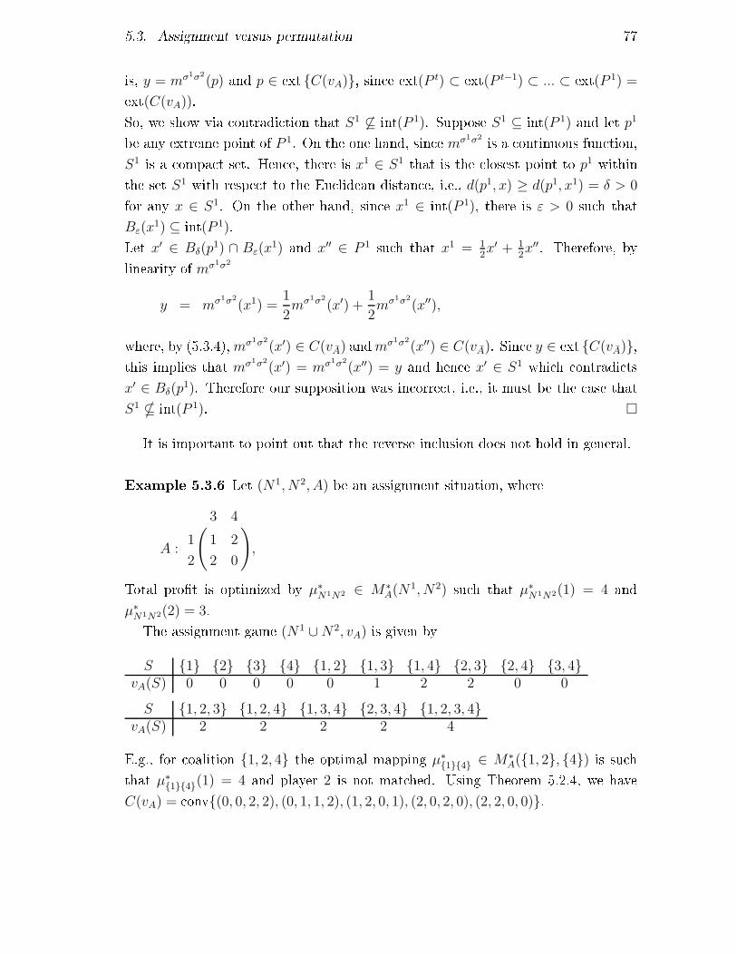
5.3. Assignment versus permutation 77is, y = mσ1σ2(p) and p ∈ ext {C(vA)}, sin e ext(P t) ⊂ ext(P t−1) ⊂ ... ⊂ ext(P 1) =ext(C(vA)).So, we show via ontradi tion that S1 6⊆ int(P 1). Suppose S1 ⊆ int(P 1) and let p1be any extreme point of P 1. On the one hand, sin e mσ1σ2 is a ontinuous fun tion,

S1 is a ompa t set. Hen e, there is x1 ∈ S1 that is the losest point to p1 withinthe set S1 with respe t to the Eu lidean distan e, i.e., d(p1, x) ≥ d(p1, x1) = δ > 0for any x ∈ S1. On the other hand, sin e x1 ∈ int(P 1), there is ε > 0 su h thatBε(x

1) ⊆ int(P 1).Let x′ ∈ Bδ(p1) ∩ Bε(x

1) and x′′ ∈ P 1 su h that x1 = 12x′ + 1

2x′′. Therefore, bylinearity of mσ1σ2

y = mσ1σ2

(x1) =1

2mσ1σ2

(x′) +1

2mσ1σ2

(x′′),where, by (5.3.4),mσ1σ2(x′) ∈ C(vA) andmσ1σ2

(x′′) ∈ C(vA). Sin e y ∈ ext {C(vA)},this implies that mσ1σ2(x′) = mσ1σ2

(x′′) = y and hen e x′ ∈ S1 whi h ontradi tsx′ ∈ Bδ(p

1). Therefore our supposition was in orre t, i.e., it must be the ase thatS1 * int(P 1). �It is important to point out that the reverse in lusion does not hold in general.Example 5.3.6 Let (N1, N2, A) be an assignment situation, where

A :

( 3 4

1 1 2

2 2 0

),Total pro�t is optimized by µ∗

N1N2 ∈ M∗A(N

1, N2) su h that µ∗N1N2(1) = 4 and

µ∗N1N2(2) = 3.The assignment game (N1 ∪N2, vA) is given byS {1} {2} {3} {4} {1, 2} {1, 3} {1, 4} {2, 3} {2, 4} {3, 4}

vA(S) 0 0 0 0 0 1 2 2 0 0

S {1, 2, 3} {1, 2, 4} {1, 3, 4} {2, 3, 4} {1, 2, 3, 4}vA(S) 2 2 2 2 4E.g., for oalition {1, 2, 4} the optimal mapping µ∗

{1}{4} ∈ M∗A({1, 2}, {4}) is su hthat µ∗

{1}{4}(1) = 4 and player 2 is not mat hed. Using Theorem 5.2.4, we haveC(vA) = onv{(0, 0, 2, 2), (0, 1, 1, 2), (1, 2, 0, 1), (2, 0, 2, 0), (2, 2, 0, 0)}.

78 Chapter 5. Mat hing situations: onne ting assignment and permutationLet N = {1, 2}, and let σ1 ∈ Π(N1, N1) and σ2 ∈ Π(N2, N2) be su h thatσ1(1) = 1, σ1(2) = 2, σ2(3) = 1, σ2(4) = 2. This results in the permutationsituation (N, N , A), with

A :

( 1 2

1 1 2

2 2 0

).For the asso iated permutation game (N, vA) we obtain:

S {1} {2} {1, 2}vA(S) 1 0 4and the ore is given by C(vA) = onv{(1, 3), (4, 0)}. Sin e (0, 0, 2, 2) ∈ ext(C(vA))but m((0, 0, 2, 2)) = (2, 2) 6∈ ext(C(vA)), we an on lude that ext {C(vA)} 6⊇

mσ1σ2(ext(C(vA))). ⊳Nevertheless, with every square assignment situation we an asso iate a permutationsituation su h that the reverse in lusion holds.Theorem 5.3.7 Let (N1, N2, A) be an assignment situation su h that |N1| = |N2|,and let N be su h that |N | = |N1|. Then there exist σ1 ∈ Π(N , N1) and σ2 ∈

Π(N, N2) su h that for the asso iated permutation situation (N , N , A) it holds thatmσ1σ2

(ext(C(vA))) = ext(C(vA)).Proof: Let µ∗N1N2 ∈ M∗

A(N1, N2). Let σ1 ∈ Π(N, N1), and let σ2 ∈ Π(N , N2)be su h that σ2(i) = µ∗

N1N2(σ1(i)) for every i ∈ N . By Theorem 5.3.5 we haveext(C(vA)) ⊆ mσ1σ2(ext(C(vA))).It remains to show that mσ1σ2

(ext(C(vA))) ⊆ ext(C(vA)). It is readily he kedthat vA is an additive game and ext(C(vA)) = C(vA) = (aii)i∈N . Let(u, v) ∈ ext(C(vA)). By Theorem 5.2.4 we have ui + vj = aij for all (i, j) ∈

µ∗N1N2 . Hen e, for every i ∈ N , mσ1σ2

i (u, v) = uσ1(i) + vσ2(i) = aσ1(i)σ2(i) =

aii. Therefore, mσ1σ2(u, v) ∈ ext(C(vA)) so mσ1σ2

(ext(C(vA))) ⊆ ext(C(vA)).�

5.3. Assignment versus permutation 795.3.2 Böhm-Bawerk mat hingAssignment situations an be used to model a two-sided market of heterogeneousgoods. The Böhm-Bawerk horse market situation (Böhm-Bawerk (1891)) is a spe- i� assignment situation where the goods traded for money are homogeneous. Ina Böhm-Bawerk assignment situation every player is hara terized by a single non-negative number: ea h buyer i ∈ N1 values a unit of the good at wi ≥ 0, whereasea h seller j ∈ N2 values her own good at cj ≥ 0. The pro�t that an be rea hedthrough a transa tion between buyer i and seller j is max {0, wi − cj}. The followingde�nition generalizes Böhm-Bawerk assignment situations.De�nition 5.3.8 Let N1, N2 be two player sets, and let w ∈ RN1

+ and c ∈ RN2

+ .Then the Böhm-Bawerk mat hing situation (N1, N2, Aw,c) is given by aw,cij =

max{0, wi − cj} for every i ∈ N1 and j ∈ N2.If (N1, N2, Aw,c) is an assignment situation, we obtain the original model byBöhm-Bawerk (1891).We expand the Böhm-Bawerk framework, but the interpretation of the Böhm-Bawerk assignment situation annot be expanded to the Böhm-Bawerk mat hingsituation, as it seems unnatural to have a player simultaneously being a seller witha low valuation of the good and a buyer with a high valuation of the good. Thefollowing is however interesting from a mathemati al point of view, as for this lassof mat hing situations both the extreme points of the ore and the nu leolus are pre-served in the translation from an assignment situation to the asso iated permutationsituation. Furthermore, with a di�erent interpretation - one an think of situationswhere pro essing the job of player i ∈ N1 on any ma hine results in a revenue of wi,and cj represents the ost of pro essing a job on the ma hine of player j ∈ N2 - theresults remain relevant.For every Böhm-Bawerk mat hing situation, we an hara terize an optimal or-der.Theorem 5.3.9 (Böhm-Bawerk (1891)) Let (N1, N2, Aw,c) be a Böhm-Bawerkmat hing situation. Then there exists a mat hing µ∗T 1T 2 ∈ M∗

Aw,c(N1, N2) su hthat wi ≥ wj for every i ∈ T 1 and every j ∈ N1\T 1, ci ≤ cj for every i ∈ T 2 andevery j ∈ N2\T 2, and, for every i, j ∈ T 1, cµ∗T1T2 (i)

≤ cµ∗T1T2 (j)

if wi > wj.

80 Chapter 5. Mat hing situations: onne ting assignment and permutationSo, for su h an optimal mat hing µ∗T 1T 2 ∈M∗

Aw,c(N1, N2), the buyer with the highestvaluation is paired to the seller with the lowest valuation, the buyer with the se ond-highest valuation is paired to the seller with the se ond-lowest valuation et .For every Böhm-Bawerk mat hing situation (N1, N2, Aw,c), we de�ne the follow-ing parameterrw,c =

∣∣∣{i ∈ N1 | aw,c

iµ∗T1T2 (i)

> 0}∣∣∣ ,where µ∗

T 1T 2 ∈ M∗Aw,c(N1, N2) is su h that it satis�es the onditions of Theorem5.3.9. Given the Böhm-Bawerk permutation game asso iated to Aw,c, rw,c is themaximum number of mat hings that an be arried out simultaneously, giving astri tly positive bene�t. To avoid the null game we assume rw,c > 0.For the ve tors w ∈ RN1 and c ∈ RN2 , we de�ne w ∈ RN1 as the ve tor thatorders the elements of w su h that w1 ≥ w2 ≥ ... ≥ wn and c ∈ RN2 as the ve torthat orders the elements of c su h that c1 ≤ c2 ≤ ... ≤ cn. Hen e, wk denotes the

kth largest omponent of w, and ck denotes the kth smallest omponent of c. Fornotational onvenien e, we take wk = −∞ if k > n and ck = ∞ if k > n.For the Böhm-Bawerk mat hing situation (N1, N2, Aw,c), we say that an agenti ∈ N1 is buyer-a tive if wi ≥ wrw,c . We denote HB ∈ 2N

1∪N2 for the set of buyer-a tive agents, and denote HBS = HB ∩ S for every S ∈ 2N

1∪N2 . We all an agenti ∈ N2 seller-a tive if ci ≤ crw,c . We denote HS ∈ 2N

1∪N2 for the set of seller-a tiveagents, and denote HSS = HS ∩ S for every S ∈ 2N

1∪N2 . A player i ∈ N1 ∩ N2 is alled a tive if he is both buyer-a tive and seller-a tive, and is alled ina tive if heis neither buyer-a tive nor seller-a tive. As the player i ∈ N su h that wi = wrw,c(as well as the player i ∈ N su h that ci = crw,c) need not be unique, the number ofa tive buyers an di�er from the number of a tive sellers.De�ne for the Böhm-Bawerk assignment situation (N1, N2, Aw,c), p, p ∈ R+ su hthatp = max {wrw,c+1, crw,c} ,p = min {wrw,c , crw,c+1} .The values for p and p are su h that the number of transa tions su h that all sellersand all buyers involved in a transa tion a hieve a non-negative value, is maximized.Given an optimal mat hing µ∗

T 1T 2 ∈ M∗Aw,c(N1, N2), a pri e p ∈ [p, p] and player

i ∈ T 1, if the value wi − cµ∗T1T2 (i)

from a transa tion between the mat hed players i

5.3. Assignment versus permutation 81and µ∗T 1T 2(i) is non-negative, then both the value wi − p that the buyer i a hievesfrom buying the good and the value p − cµ∗

T1T2 (i)that the seller µ∗

T 1T 2(i) a hievesfrom selling the good are non-negative.For Böhm-Bawerk assignment games, the reverse in lusion of Theorem 5.2.5 alsoholds: the ore is a line segment de�ned by (u, v) and (u, v). Moreover, we anprovide expressions for u, u, v and v in terms of w and c.Theorem 5.3.10 (Shapley and Shubik (1972), Moulin (1996)) Let (N1, N2, Aw,c)be a Böhm-Bawerk assignment situation. Then C(vAw,c) = onv{(u, v), (u, v)} with,for every i ∈ N1,ui =

{wi − p if i ∈ HB

0 if i ∈ N1\HBand ui = {wi − p if i ∈ HB

0 if i ∈ N1\HB.And, for every i ∈ N2,vi =

{p− ci if i ∈ HS

0 if i ∈ N2\HSand vi = {p− ci if i ∈ HS

0 if i ∈ N2\HS.Using Theorem 5.3.4 and Theorem 5.3.10, it is straightforward to express the ore of a Böhm-Bawerk permutation game in terms of the valuations of the players.Theorem 5.3.11 Let (N,N,Aw,c) be a Böhm-Bawerk permutation game. ThenC(vAw,c) = {y(p) | p ≤ p ≤ p} where

y(p)i =

wi − ci if i ∈ HB ∩HS

wi − p if i ∈ HB\HS

p− ci if i ∈ HS\HB

0 if i ∈ N\(HB ∪HS),for every p ∈ [p, p] and every i ∈ N .Proof: The expression follows dire tly from Theorem 5.3.4 and Theorem 5.3.10.�Observe that an a tive agent does not bene�t from ooperation, sin e he re eiveshis stand alone value at any ore allo ation, but only agents that are either buyer-a tive or seller-a tive (and not both) do. As it should be expe ted the interests of

82 Chapter 5. Mat hing situations: onne ting assignment and permutationall agents that are only buyer-a tive are totally aligned and opposed to the interestsof all agents that are only seller-a tive, and vi e versa.Now, we turn to the preservation of distin t points of the ore. First of all, we onsider the extreme points of the ore.Theorem 5.3.12 Let (N1, N2, Aw,c) be a square Böhm-Bawerk assignment sit-uation, let N be su h that |N | = |N1|. Then for any σ1 ∈ Π(N, N1) andσ2 ∈ Π(N , N2), it holds for permutation situation (N , N , Aw,c) that ext {C(vAw,c)} =

mσ1σ2(ext {C(vAw,c)}).Proof: By Theorem 5.3.10, we have ext(C(vAw,c) = {(u, v), (u, v)}. It is readily he ked that mσ1σ2

(u, v) = y(p) and mσ1σ2(u, v) = y(p), so by Theorem 5.3.11 thestatement follows. �Note the dis repan y with Theorem 5.3.7. For a general square assignment situ-ation, there exist an asso iated permutation situation su h that the extreme pointsof the ore are preserved in the translation from the ore of the assignment game tothe ore of the permutation game. For the spe ial ase of Böhm-Bawerk assignmentsituations however, this holds for every asso iated permutation situation.Now, we turn to the nu leolus. For Böhm-Bawerk assignment games Núñez andRafels (2005) show that the nu leolus oin ides with the bary enter of the ore.Theorem 5.3.13 (Núñez and Rafels (2005)) Let (N1, N2, Aw,c) be a Böhm-Bawerkassignment situation. Then

η(N, vAw,c) =1

2(u, v) +

1

2(u, v).We provide an expli it expression for the nu leolus of a Böhm-Bawerk permuta-tion game.Theorem 5.3.14 Let (N,N,Aw,c) be a Böhm-Bawerk permutation situation. Then

η(N, vAw,c) = y

(1

2p+

1

2p

).

5.3. Assignment versus permutation 83Proof: First, if wrw,c = wrw,c+1, p = min{wrw,c+1, crw,c+1} = wrw,c+1 and p =

max{wrw,c , crw,c} = wrw,c . Hen e, p = p. Therefore, the ore C(vAw,c) is a singletonand the statement follows. If crw,c = crw,c+1, a similar argument shows that C(vAw,c)is a singleton. So, we assume wrw,c > wrw,c+1 and crw,c < crw,c+1. This means that|HS| = |HB|. If HS = HB, then C(vAw,c) is a singleton and the statement follows.So, we assume |HS| = |HB| and HS\HB 6= ∅ (and therefore HB\HS 6= ∅).The stru ture of the proof is as follows: �rst, we show that for every oalition withthe same number of a tive sellers and a tive buyers the ex ess is 0 for every oreelement. Then, we demonstrate that there are two spe ial oalitions su h that forevery ore element the highest ex ess that is not onstant a ross all ore elements, isattained by one of these two oalitions. hen e, the ex ess ve tor is lexi ographi allyminimized, if the maximum of the ex ess of these two oalitions is minimized.For every S ∈ 2N , de�ne σB

S ∈ Π(S) and σSS ∈ Π(S) su h that wσB

S(k) ≥ wσB

S(k+1)and cσS

S(k) ≤ cσS

S(k+1) for every k ∈ {1, ..., |S|−1}. Note that for every S ∈ 2N , thereexists a µ∗

SS ∈M∗Aw,c(S, S) su h that µ∗

SS(σBS (k)) = σS

S (k) for every k ∈ {1, ..., |S|}.Take p ∈ [p, p]. First, we show that E(S, y(p)) = 0 if |HSS | = |HB

S |. So, let S ∈ 2Nbe su h that |HSS | = |HB

S |. We haveE(S, y(p)) + v(S)−

∑

i∈S

yi(p)

=

|HSS|∑

t=1

(wσBS(t) − cσS

S(t))−

∑

i∈HSS∩HB

S

(wi − ci)

−∑

i∈HSS\HB

S

(p− ci)−∑

i∈HBS\HS

S

(wi − p)

= 0.So, for every oalition S ∈ 2N with |HSS | = |HB

S | the ex ess E(S, y(p)) is independentof p.Now, we provide upper bounds for the ex ess of oalitions S ∈ 2N su h that |HBS | 6=

|HSS | and show that these upper bounds are attained by some oalition.• |HB

S | > |HSS |. We obtain the following expression for the ex ess E(S, y(p)):

84 Chapter 5. Mat hing situations: onne ting assignment and permutationE(S, y(p)) = v(S)−

∑

i∈S

yi(p)

=

|HSS|∑

t=1

(wσBS(t) − cσS

S(t)) +

|HBS|∑

t=|HSS|+1

max{wσBS(t) − cσS

S(t), 0}

−∑

i∈HSS∩HB

S

(wi − ci)−∑

i∈HSS\HB

S

(p− ci)−∑

i∈HBS\HS

S

(wi − p)

=

|HSS |∑

t=1

(wσBS(t) − cσS

S(t)) +

|HBS |∑

t=|HSS|+1

max{wσBS(t) − cσS

S(t), 0}

−∑

i∈HSS

(p− ci)−∑

i∈HBS

(wi − p)

=

|HBS|∑

t=|HSS|+1

(max{wσBS(t) − cσS

S(t), 0} − (wσB

S(t) − p))

=

|HBS |∑

t=|HSS|+1

(max{p− cσSS(t), p− wσB

S(t)})

≤ max{p− crw,c+1, p− wrw,c},

where the fourth equality follows from the fa t that σBS (t) ∈ HB

S andσSS (t) ∈ HS

S for every t ∈ {1, ..., |HSS |}. The inequality follows from the obser-vation that, for every t ∈ {|HS

S | + 1, ..., |HBS |}, max{p − cσS

S(t), p − wσB

S(t)} ≤

max{p − crw,c+1, p − wrw,c} ≤ 0 as crw,c+1 ≤ cσSS(t), wrw,c ≤ wσB

S(t) and

p ≤ p = min{wrw,c , crw,c+1}.We show that there a tually exists a oalition S ∈ 2N su h that E(S, y(p)) =max{p − crw,c+1, p − wrw,c}. Take i ∈ N su h that wi = wrw,c and j ∈ Nsu h that cj = crw,c+1. Obviously i ∈ HB and j 6∈ HS. If i = j, then learlyE({i}, y(p)) = max{wrw,c−crw,c+1, 0}−(wrw,c−p) = max{p−crw,c+1, p−wrw,c}.If i 6= j, we distinguish the following ases:(A) i ∈ HS and j ∈ HB. Consider S = {i, j}. We have σB

S (1) = j, σBS (2) = i,

σSS (1) = i, σS

S (2) = j, so

5.3. Assignment versus permutation 85E(S, y(p)) = (wrw,c − crw,c+1)−max{wj − ci, 0}

−(wrw,c − ci)− (wj − p)

= max{p− crw,c+1, p− wrw,c}.(B) i ∈ HS and j 6∈ HB. Let h ∈ HB\HS, and take S = {h, i, j}. NowσBS (1) = h, σB

S (2) = i, σBS (3) = j, σS

S(1) = i, σSS (2) = j, σS

S (3) = h, soE(S, y(p)) = (wh − ci) + max{wrw,c − crw,c+1, 0}

−(wh − p)− (wrw,c − ci)

= max{p− crw,c+1, p− wrw,c}.(C) i 6∈ HS and j ∈ HB. Similar to (B), let h ∈ HS\HB, and take S =

{h, i, j}. Now σBS (1) = j, σB

S (2) = i, σBS (3) = h, σS

S (1) = h, σSS(2) = i,

σSS(3) = j, so

E(S, y(p)) = (wj − ch) + max{wrw,c − crw,c+1, 0}

−(wrw,c − p)− (wj − p)− (p− ch)

= max{p− crw,c+1, p− wrw,c}.(D) i 6∈ HS and j 6∈ HB. Consider S = {i, j}. We have σBS (1) = i, σB

S (2) = j,σSS(1) = j, σS

S (2) = i, soE(S, y(p)) = max{wrw,c − crw,c+1, 0} − (wrw,c − p)

= max{p− crw,c+1, p− wrw,c}.So, for every oalition S ∈ 2N su h that |HBS | > |HS

S |,E(S, y(p)) ≤ max{p− crw,c+1, p− wrw,c},with equality for at least one su h S.

• |HSS | > |HB

S |. We obtain the following expression for the ex ess E(S, y(p)):

86 Chapter 5. Mat hing situations: onne ting assignment and permutationE(S, y(p)) + v(S)−

∑

i∈S

yi(p)

=

|HBS|∑

t=1

(wσBS(t) − cσS

S(t)) +

|HSS|∑

t=|HBS|+1

max{wσBS(t) − cσS

S(t), 0}

−∑

i∈HSS∩HB

S

(wi − ci)−∑

i∈HSS\HB

S

(p− ci)−∑

i∈HBS\HS

S

(wi − p)

=

|HBS |∑

t=1

(wσBS(t) − cσS

S(t)) +

|HSS |∑

t=|HBS|+1

max{wσBS(t) − cσS

S(t), 0}

−∑

i∈HSS

(p− ci)−∑

i∈HBS

(wi − p)

=

|HSS|∑

t=|HBS|+1

(max{wσBS(t) − cσS

S(t), 0} − (p− cσB

S(t)))

=

|HSS |∑

t=|HBS|+1

(max{cσSS(t) − p, wσB

S(t) − p})

≤ max{wrw,c+1 − p, crw,c − p},where the fourth equality follows from the fa t that σBS (t) ∈ HB

S andσSS (t) ∈ HS

S for every t ∈ {1, ..., |HBS |}. The inequality follows from the obser-vation that, for every t ∈ {|HB

S | + 1, ..., |HSS |}, max{wσB

S(t) − p, cσS

S(t) − p} ≤

max{wrw,c+1 − p, crw,c − p} ≤ 0 as crw,c ≥ cσSS(t), wrw,c+1 ≥ wσB

S(t) and

p ≥ p = max{wrw,c+1, crw,c}.We show that there a tually exists a oalition S ∈ 2N su h that E(S, y(p)) =max{wrw,c+1 − p, crw,c − p}. Take i ∈ N su h that wi = wrw,c+1 and j ∈ Nsu h that cj = crw,c . Obviously i 6∈ HB and j ∈ HS. If i = j, then learlyE({i}, y(p)) = max{wrw,c+1− crw,c , 0}−(p− crw,c) = max{wrw,c+1−p, crw,c−p}.If i 6= j, we distinguish the following ases:(A) i ∈ HS and j ∈ HB. Consider S = {i, j}. We have σB

S (1) = j, σBS (2) = i,

σSS (1) = i, σS

S (2) = j, soE(S, y(p)) = (wj − ci) + max{wrw,c+1 − crw,c , 0} − (p− ci)− (wj − crw,c)

= max{wrw,c+1 − p, crw,c − p}.

5.3. Assignment versus permutation 87(B) i ∈ HS and j 6∈ HB. Let h ∈ HB\HS, and take S = {h, i, j}. NowσBS (1) = h, σB

S (2) = i, σBS (3) = j, σS

S(1) = i, σSS (2) = j, σS

S (3) = h, soE(S, y(p)) = (wh − ci) + max{wrw,c+1 − crw,c , 0}

−(wh − p)− (p− ci)− (p− crw,c)

= max{wrw,c+1 − p, crw,c − p}.(C) i 6∈ HS and j ∈ HB. Similar to (B), let h ∈ HS\HB, and take S =

{h, i, j}. Now σBS (1) = j, σB

S (2) = i, σBS (3) = h, σS

S (1) = h, σSS(2) = i,

σSS(3) = j, soE(S, y(p)) = (wj − ch) + max{wrw,c+1 − crw,c , 0} − (wi − crw,c)− (p− ch)

= max{wrw,c+1 − p, crw,c − p}.(D) i 6∈ HS and j 6∈ HB. Consider S = {i, j}. We have σBS (1) = i, σB

S (2) = j,σSS(1) = j, σS

S (2) = i, soE(S, y(p)) = max{wrw,c − crw,c+1, 0} − (p− crw,c+1)

= max{wrw,c+1 − p, crw,c − p}.So, for every oalition S ∈ 2N su h that |HSS | > |HB

S |,E(S, y(p)) ≤ max{wrw,c+1 − p, crw,c − p},with equality for at least one su h S.Take S1, S2 ∈ 2N su h that, for every p ∈ [p, p], E(S1, y(p)) = max{p− crw,c+1, p−

wrw,c} and E(S2, y(p)) = max{wrw,c+1 − p, crw,c − p}. Irrespe tive of the hoi e ofp ∈ [p, p],

maxS∈2N s.t. |HB

S|6=|HS

S|{E(S, y(p))} = max{E(S1, y(p)), E(S2, y(p))}.Sin e

88 Chapter 5. Mat hing situations: onne ting assignment and permutationE(S1, y(p)) + E(S2, y(p)) = max{p− crw,c+1, p− wrw,c}

+max{wrw,c+1 − p, crw,c − p}

= max{wrw,c+1, crw,c} −min{crw,c+1, wrw,c}

= p− p,is onstant, the ex ess ve tor of y(p) is lexi ographi ally minimized if E(S1, y(p)) =

E(S2, y(p)). Hen e, for the nu leolus η(vAw,c) it must hold thatE(S1, η(vAw,c)) = E(S2, η(vAw,c)) =

1

2(p− p).So, we obtain

p = E(S1, η(vAw,c))−max{−crw,c+1,−wrw,c}

=1

2(p− p) + min{crw,c+1, wrw,c}

=1

2(max{wrw,c+1, crw,c} −min{crw,c+1, wrw,c}) + min{crw,c+1, wrw,c}

=1

2(p+ p).Hen e, η(vAw,c) = y(1

2(p+ p)). �The next orollary now follows from Theorem 5.3.13 and 5.3.14.Corollary 5.3.15 Let (N1, N2, Aw,c) be a square Böhm-Bawerk assignment situa-tion, let N be su h that |N | = |N1| and take σ1 ∈ Π(N, N1), σ2 ∈ Π(N, N2). Thenfor the Böhm-Bawerk permutation situation (N, N , Aw,c) it holds that η(vAw,c) =

mσ1σ2(η(vAw,c).To obtain the results of Theorem 5.3.14 and Corollary 5.3.15, we suggest as anotherproof approa h to use the results by Solymosi et al. (2005) on y li permutationsituations and the pair-nu leolus and the proof that Núñez and Rafels (2005) providefor Theorem 5.3.13.5.4 Permutation situations and gamesIn the last part of this hapter, our main fo us is on permutation situations. Weanalyze the set of undominated matri es for permutation situations: given a per-mutation situation, the set of undominated matri es is formed by those matri es

5.4. Permutation situations and games 89leading to the same permutation game for whi h we annot raise any entry of thematrix without hanging the ore. Martínez-Albéniz et al. (2011) hara terized theset of undominated matri es for assignment situations. Before we present our resultson the set of undominated matri es for permutation situations, we will brie�y repeattheir results. Se ond, we dis uss a sub lass of the lass of permutation situations.For these permutation situations, we hara terize optimal mat hings and provideexpli it expressions for both the ore and the nu leolus.5.4.1 The ore and exa tnessFirst, we introdu e two sets of matri es.De�nition 5.4.1 Let (N1, N2, A) be a mat hing situation. Then the set of matri esgenerating C(vA) is given by G(A) = {B ∈ M+N1×N2 | C(vA) = C(vB)}.For A,B ∈ M+

N1×N2 , we denote A ≥ B if aij ≥ bij for every i ∈ N1, j ∈ N2.De�nition 5.4.2 Let (N1, N2, A) be a mat hing situation. Then the set of un-dominated matri es generating C(vA) is given by U(A) = {B ∈ G(A) | ∄C ∈

G(A)\{B} su h that C ≥ B}.We illustrate the above de�nitions with the following example.Example 5.4.3 Let (N,N,A) and (N,N,B(α, β)) be permutation situations,whereA :

( 1 2

1 1 0

2 0 1

) and B(α, β) :

( 1 2

1 1 α

2 β 1

),for every α, β ∈ R+. We have C(vA) = {(1, 1)}. For a balan ed 2-person game

(N, v) it holds thatC(v) = onv{(v({1}), v({1, 2})− v({1})), (v({1, 2})− v({2}), v({2}))}.So, for every game (N, v) su h that C(v) = C(vA) it must hold that v({1}) =

v({2}) = 1 and v({1, 2}) = 2. Hen e,

90 Chapter 5. Mat hing situations: onne ting assignment and permutationG(A) = {B(α, β) | α + β ≤ 2 and α, β ≥ 0}andU(A) = {B(α, β) | α + β = 2 and α, β ≥ 0}.

⊳For every assignment situation (N1, N2, A), Martínez-Albéniz et al. (2011) har-a terize both G(A) and U(A). In fa t, they show that G(A) onsists of a �niteunion of onvex sets. In ase that the optimal mat hing for the grand oalition isunique, G(A) onsists of one onvex set. Also, they show that U(A) is a singleton,and the unique element of U(A) is the unique matrix in G(A) that orresponds witha buyer-seller exa t assignment game. Here, an assignment game (N1 ∪ N2, vA) is alled buyer-seller exa t (Núñez and Rafels (2002)) if for every i ∈ N1, j ∈ N2, thereexists a (u, v) ∈ C(vA) su h that ui + vj = vA({i, j})).Note that there does not need to exist a matrix B ∈ G(A) su h that (N1∪N2, vB)is exa t, as the following example demonstrates.Example 5.4.4 (Núñez and Rafels (2002)) Consider the assignment situation(N1, N2, A), where N1 = {1, 2, 3}, N2 = {4, 5, 6} and A is given by

A :

4 5 6

1 5 8 3

2 7 9 6

3 2 3 0

.The ore of the assignment game (N, vA) is given by C(vA) = {((3, 5, 0), (2, 5, 1)),

((5, 6, 1), (1, 3, 0)), ((3, 6, 0), (2, 5, 0)), ((4, 6, 1), (1, 4, 0)), ((5, 6, 0), (2, 3, 0)), ((4, 5, 0),

(2, 4, 1))}. It is readily he ked that (N, vA) is buyer-seller exa t, hen e, U(A) =

{A}. As every exa t assignment game is buyer-seller exa t, this also means thatif there exists a matrix B ∈ G(A) su h that (N1 ∪ N2, vB) is exa t, it must holdthat B = A. However, vA({1}) = 0 but min(u,v)∈C(vA) u1 = 3. Hen e, (N, vA) is notexa t. ⊳For every permutation situation (N,N,A) with |N | ≤ 3 however, we an showthat not only there exists a matrix B ∈ U(A) su h that (N, vB) is exa t, but thisholds for every matrix B ∈ U(A).

5.4. Permutation situations and games 91For every permutation situation (N,N,A) and every i, j ∈ N , de�neSijA =

{S ∈ 2N | vA(S) = min

y∈C(vA)y(S), and µ∗

SS(i) = j for some µ∗SS ∈M∗

A(S, S)

}.So, if S ∈ Sij

A , then raising the entry aij would raise vA(S) and hange the ore of(N, vA).Theorem 5.4.5 Let (N,N,A) be a permutation situation, with n ≤ 3. Then(N, vB) is an exa t game for all B ∈ U(A).Proof: The ases where n = 1 and n = 2 are trivial, as for n < 3 every balan edgame is exa t. Hen e, let n = 3 and suppose that (N, vB) is not exa t for someB ∈ U(A), i.e., there is U ( N su h that vB(U) < minx∈C(vB) x(U). We distinguishtwo ases.Case 1: |U | = 1.De�ne Br ∈ M+

N1×N2 bybrij = bij for all i ∈ N, j ∈ N\{i},

brii = minx∈C(vB) xi for all i ∈ N.Observe that Br ≥ B, as bii ≤ vB({i}) for every i ∈ N with at least one stri tinequality.We show that C(vBr) = C(vB), whi h ontradi ts B ∈ U(A). First we showC(vBr) ⊆ C(vB). Trivially,

vBr(S) ≥ vB(S) for all S ∈ 2N . (5.2)Let µNN ∈ M∗Br(N,N). We take S, T ∈ 2N su h that S ∪ T = N , µN,N(i) = i forevery i ∈ S and µN,N(i) 6= i for every i ∈ T . Then

vBr(N) =∑

i∈S

briµNN (i) +∑

i∈T

briµNN (i)

≤∑

i∈S

minx∈C(vB)

xi + vB(T )

≤ minx∈C(vB)

{x(S)}+ minx∈C(vB)

{x(T )}

≤ minx∈C(vB)

x(N) = vB(N) ≤ vBr(N).

92 Chapter 5. Mat hing situations: onne ting assignment and permutationThus vBr(N) = vB(N), whi h, together with (5.2), implies that C(vBr) ⊆ C(vB).Next we show C(vB) ⊆ C(vBr). Let x ∈ C(vB). By onstru tion ofBr, xi ≥ vBr({i})for every i ∈ N . Take i ∈ N , j ∈ N\{i}, take S = {i, j} and µSS ∈ M∗Br(S, S). If

µSS(i) = i and µSS(j) = j then by de�nition of brii and brjj ,vBr(S) = brii + brjj ≤ xi + xj .If µSS(i) = j and µSS(j) = i then by onstru tion of Br,vBr(S) = bij + bji = vB(S) ≤ xi + xj ,as x ∈ C(vB). Therefore, C(vBr) = C(vB) = C(vA). In on lusion, Br ∈ U(A),

Br ≥ B and Br 6= B, whi h is a ontradi tion with B ∈ U(A).Case 2: |U | = 2.Take i, j ∈ N su h that U = {i, j} and let k ∈ N\{i, j}. By assumption,vB(U) = max{bii + bjj , bij + bji} < min

x∈C(vB)xi + xj . (5.3)Sin e B ∈ U(A), we annot in rease bij and bji without hanging the ore of the orresponding permutation game. Hen e, there exists an Sij ∈ Sij

B . Sin e vB(U) <minx∈C(vB)(xi + xj) and n = 3, we ne essarily have S(i,j) = {i, j, k}. Note thatvB(N) = bij + bji + bkk would imply that xk = bkk for all x ∈ C(vB). This impliesvB(U) = xi + xj = minz∈C(vB) z(U), whi h ontradi ts (5.3). Therefore

vB(N) = bij + bjk + bki = x(N), (5.4)for all x ∈ C(vB).Analogously, with Sji ∈ Sij we obtainvB(N) = bji + bik + bkj = x(N), (5.5)for all x ∈ C(vB). From (5.4) and (5.5), for all x ∈ C(vB),2vB(N) = (bij + bjk + bki) + (bji + bik + bkj)

= (bij + bji) + (bik + bki) + (bjk + bkj)

≤ vB ({i, j}) + vB ({i, k}) + vB ({j, k})

< 2x(N)

= 2vB(N),

5.4. Permutation situations and games 93a ontradi tion. Note that the stri t inequality holds by (5.3) and the last inequalityholds sin e x ∈ C(vB). �The proof of the above result ould be simpli�ed a little bit by further exploitingthe ri her stru ture of the three-player set ase. However, we have hosen this moregeneral proof for it ould guide the reader to understand (and maybe solve) thegeneral ase. Be ause of the unsu essful sear h of ounterexamples we onje turethat the result of Theorem 5.4.5 may hold in the general ase, i.e, for an arbitraryplayer set. Note that for games with at most three players, every exa tness isequivalent with onvexity. Hen e, every undominated matrix results in a onvexgame. We on lude this part with the following example, whi h shows that U(A) an onsist of more than one onvex set.Example 5.4.6 Consider the permutation situations (N,N,A) and (N,N,B)where N = {1, 2, 3} and A and B are given byA :

1 2 3

1 1 3 0

2 0 2 3

3 3 0 0

and B :

1 2 3

1 1 0 3

2 3 2 0

3 0 3 0

.These matri es both lead to the following permutation game

S {1} {2} {3} {1, 2} {1, 3} {2, 3} {1, 2, 3}vA(S) 1 2 0 3 3 3 9with C(v) = onv{(1, 2, 6), (1, 6, 2), (3, 6, 0), (6, 2, 1), (6, 3, 0)}. Note that (N, vA)is exa t, so we annot raise the value of any oalition without hanging the ore.Any matrix C ∈ G(A) must satisfy the following inequalities:

c11 ≤ 1 c12 + c21 ≤ 3

c22 ≤ 2 c13 + c31 ≤ 3

c33 ≤ 0 c23 + c32 ≤ 3As vA(N) = 9, these onditions imply that no entry of C is larger than 3, and that

94 Chapter 5. Mat hing situations: onne ting assignment and permutationno entry on the diagonal an be used in an optimal mat hing for N . Hen e, eitherc12 = c23 = c31 = 3 (and therefore c21 = c32 = c13 = 0) or c13 = c32 = c21 = 3(and therefore c31 = c23 = c12 = 0). Also, to ensure that (1, 2, 6) ∈ ext(C(vC)) and(1 + a, 2− a, 6) 6∈ C(vC) for every a ∈ [−1, 0) ∪ (0, 2], it must hold that c11 = 1 andc22 = 2. Together, this shows that G(A) = G(B) = {A,B}. Also, for both A and B,every entry is used in an optimal mat hing for some oalition S ∈ N : e.g., the entrya(1,3) is used in the optimal mat hing for oalition {1, 3}. Hen e, the matri es Aand B are undominated: U(A) = U(B) = {A,B}. Note that B = A⊤. In fa t it iseasily seen that if a matrix is undominated, then also its transpose is undominated.⊳5.4.2 `Homogeneous alternatives' permutationNow, we analyze a sub lass of the lass of permutation situations. In this lass ofpermutation situations, every player onsiders the obje ts of the other players tobe homogeneous. So, a player either prefers the status quo or prefers any otherobje t to his own. This an be represented by two ve tors α, β ∈ RN

+ su h that αirepresents the valuation of player i ∈ N of his own obje t, and βi represents thevaluation of player i ∈ N of the other obje ts.De�nition 5.4.7 Let α, β ∈ RN+ . Then the `homogeneous alternatives' (HA) per-mutation situation (N,N,Aαβ) is given by

a(i,j) =

{αi if i = j,

βi if i 6= j,(5.6)for every i, j ∈ N .To be able to provide expressions for the ore of the permutation game, we �rst hara terize the optimal mat hings. To this end, we �rst introdu e some notation.Let (N,N,Aαβ) be a HA-permutation situation. We de�ne two sets: I = {i ∈ N |

βi < αi} and C = {i ∈ N | βi ≥ αi}. The set I represents the `individuals': thoseplayers that stri tly prefer to keep their own obje t. The set C on the other handrepresents the ` ooperators', being the players that would pro�t from swit hingobje ts with another player. For these sets, we take β = min{βk | k ∈ C} and

5.4. Permutation situations and games 95α = min{αi | i ∈ I}. We de�ne two spe ial permutations: µ0

NN ∈ M(N,N) is su hthat for every i ∈ N , µ0NN(i) = i. Furthermore, for i ∈ N , j ∈ N\{i}, we de�ne

µ(i,j)NN ∈ M(N,N) su h that µ(i,j)

NN (i) = j, µ(i,j)NN (j) = i and µ

(i,j)NN (k) = k for every

k ∈ N\{i, j}. So, µ0NN is the permutation that assigns everyone his own obje t, and

µ(i,j)NN is the permutation where only player i and j swit h obje ts. Also, let I∗ ⊆ Ibe given by I∗ = {i∗ ∈ I | αi∗ − βi∗ ≤ αi − βi for every i ∈ I}. So, I∗ ontains thoseplayers of I that are most willing to swit h obje ts. Lastly, for every S ∈ 2N , letdS ∈ R be given by

dS =

{mini∈S

{αi − βi} if S 6= ∅

0 if S = ∅Theorem 5.4.8 Let (N,N,Aαβ) be a HA-permutation situation su h that |C| 6= 1.Then µNN ∈ M∗Aαβ(N,N) if and only if µNN(i) = i for every i ∈ I and µNN(k) ∈

C\{k} for all k ∈ C su h that βk − αk > 0.Proof: Let µNN ∈M(N,N) be su h that µNN(i) = i for every i ∈ I and µNN(k) ∈

C\{k} for all k ∈ C su h that βk − αk > 0. As |C| 6= 1, su h a µNN exists. Wehave for every i ∈ N , a(i,µNN (i)) ≥ a(i,j) for every j ∈ N . Hen e, ∑i∈N a(i,µNN (i)) ≥∑i∈N a(i,µ′

NN(i)) for every µ′

NN ∈M(N,N). Hen e, µNN ∈ M∗Aαβ(N,N).For every µ′

NN ∈ M(N,N) that does not satisfy the onditions in the theorem, itholds that a(i,µ′NN

(i)) < a(i,µNN (i)) for some i ∈ N , and a(j,µ′NN

(j)) ≤ a(j,µNN (j)) for allj ∈ N\{i}. Then, ∑i∈N a(i,µNN (i) <

∑i∈N a(i,µ′

NN(i)) and µ′

NN is not optimal. �Theorem 5.4.9 Let (N,N,Aαβ) be an HA-permutation situation su h that |C| = 1and n ≥ 2. ThenM∗

Aαβ(N,N) =

{µ0NN} if dI > βk − αk,

{µ0NN} ∪ {µ(i∗,k)

NN }i∗∈I∗ if dI = βk − αk,

{µ(i∗,k)NN }i∗∈I∗ if dI < βk − αk,where k ∈ C.Proof: Let µNN ∈M(N,N). We have∑i∈N aiµNN (i) ≤

∑i∈N\{k} αi+max{αk, βk−

dI}, with equality if and only if a(i∗,µNN (i∗)) + a(k,µNN (k)) = max{αk + αi∗ , βk + βi∗},where i∗ ∈ I∗. This implies the stated expression for M∗Aαβ(N,N). �

96 Chapter 5. Mat hing situations: onne ting assignment and permutationNow, we will provide expli it expressions for the ore of the HA-permutationgame. Restri ting ourselves here to HA-matri es adds a lot of stru ture. In several ases, the ore is a singleton.Theorem 5.4.10 Let (N,N,Aαβ) be an HA-permutation situation su h that either|C| ≥ 3 or |C| = 0. Then C(vA) = {x} where

xi =

{αi if i ∈ I,

βi if i ∈ C,for every i ∈ N .Proof: If |C| = 0 thenM∗Aαβ(N,N) = {µ0

NN} and therefore vA({i})+vA(N\{i}) =

vA(N) for every i ∈ N . This implies that C(vA) = {x} where xi = vA({i}) = αi forevery i ∈ N .If |C| ≥ 3, then for i ∈ I it holds that vA({i}) + vA(N\{i}) = vA(N), so xi = αifor every i ∈ I. Take k ∈ C and divide C\{k} into two arbitrary non-emptysets C1 and C2. As |C| ≥ 3, this is possible. Sin e vA(C) = x(C) =∑

k∈C βkfor every x ∈ C(vA) we obtain via x(C) + xk ≥ vA(C1 ∪ {k}) + vA(C

2 ∪ {k}) =∑l∈C1 βl + βk +

∑l∈C2 βl + βk =

∑l∈C βl + βk that xk = βk for every k ∈ C. Hen e,

C(vA) = {x} where xi = αi for every i ∈ I and xk = βk for every k ∈ C. �In the ase where |C| = 2, the ore of the permutation game is a segment. Still,for every player in I the allo ation is equal a ross all elements of the ore, but theplayers in C an share the pro�t from ex hanging their obje ts in more than oneway.Theorem 5.4.11 Let (N,N,Aαβ) be an HA-permutation situation su h that |C| =2. Then C(vA) = onv{ck ∈ RN | k ∈ C}, where, for all k ∈ C and l ∈ N ,

ckl =

αl if l ∈ I,

max{αk, βk − dI} if l = k,

βk + βl −max{αk, βk − dI} if l ∈ C\{k}.Proof: Assume |I| = 0. It is readily he ked that the standard expression forthe ore of a 2-person game redu es to the provided expression for the ore. Nowassume |I| > 0.

5.4. Permutation situations and games 97First, we show that C(vA) ⊆ onv{ck ∈ RN | k ∈ C}. Let µ∗N,N ∈ M∗

Aαβ(N,N) andlet x ∈ C(vA). Sin e µ∗N,N(i) = i for all i ∈ I, we obtain that vA({i})+vA(N\{i}) =

v(N), and therefore xi = vA({i}). Let C = {l, k}. We have µ∗N,N(l) = k and

µ∗N,N(k) = l. So, xl + xk = βl + βk. Via vA(i, k) = max{αi + αk, βi + βk} we obtainxk ≥ max{αk, βi+βk−αi} for every k ∈ C and i ∈ I. Hen e, xk ≥ max{αk, βk−dI}.So, C(vA) ⊆ onv{ck ∈ RN | k ∈ C}.On the other hand, it is easily veri�ed that onv{ck ∈ RN | k ∈ C} ⊆ C(vA). Hen e,C(vA) = onv{ck ∈ RN | k ∈ C}. �If |C| = 1, there are two distin t situations. In the �rst ase, it is not optimal fora player in I to ex hange obje ts with the player in C, so the ore is a singleton. These ond ase is in fa t similar to Theorem 5.4.11, where the player in I∗ ex hangeshis obje t with the player in C instead of - the now non-existent - se ond player inC.Theorem 5.4.12 Let (N,N,Aαβ) be an HA-permutation situation su h that |C| =1 and |I| > 0. If |I∗| > 1, or dI ≥ βk − αk for k ∈ C, then C(vA) = {y} where

yi =

{αi if i ∈ I, or i ∈ C and dI ≥ βi − αi

βi −min{αj − βj | j ∈ I} if i ∈ C and |I∗| > 1.Proof: Assume |C| = 1 and dI ≥ βk−αk, let x ∈ C(vA). By Theorem 5.4.9, we haveµ0NN ∈M∗

Aαβ(N,N). Hen e, for every i ∈ N we have vA({i}) + vA(N\{i}) = vA(N)and therefore xi = vA({i}) = yi for every i ∈ N . Hen e, C(vA) ⊆ {y}. As the oreof a permutation game is non-empty, it follows that C(vA) = {y}.Now take dI < βk−αk and I∗ > 1, let x ∈ C(vA). The impli ation of |I∗| > 1 is that(N\{i})∩I∗ 6= ∅ for every i ∈ I. This means that vA(N\{i}) =

∑j∈N\{i} αj−dI+βkfor every i ∈ I. Therefore, for every i ∈ I it holds vA({i}) + vA(N\{i}) = vA(N)and xi = vA({i}) = yi for every i ∈ N . This means xk = βk − dI = yk. Hen e,

C(vA) ⊆ {y}. As the ore of a permutation game is non-empty, it follows thatC(vA) = {y}. �Theorem 5.4.13 Let (N,N,Aαβ) be an HA-permutation situation su h that |C| =1, |I| > 0, |I∗| = 1 and dI < βk − αk for k ∈ C. Then x ∈ C(vA) if and only if

98 Chapter 5. Mat hing situations: onne ting assignment and permutationxi = αi for all i ∈ I\I∗, xi∗ ∈ [αi∗ , βk + βi∗ −max{αk, βk −min{αi − βi | i ∈ I\I∗}}]and xk = βi + βk − xi∗ for i∗ ∈ I∗ and k ∈ C.Proof: For the `if'-part, it is readily he ked that ∑i∈S xi ≥ vA(S) for everyS ⊆ N .For the `only if'-part, assume x ∈ C(vA). Take i∗ ∈ I∗ and k ∈ C. We have thatµNN(i) = i, and therefore xi = αi for every i ∈ I\I∗. As xk ≥ vA({i, k}) − xi =

max{αi + αk, βi + βk} − αi = max{αk, βi + βk − αi} for every i ∈ I\I∗, we obtainvia xi∗ ≥ αi∗ and xi∗ + xk = vA({i∗, k}) = βk + βi∗ that xi∗ ∈ [αi, βk + βi −

max{αl,maxj∈I\DIβj − αj + βk}]. �The following theorem shows that for every HA-permutation game, the nu leolus oin ides with the bary enter of the ore.Theorem 5.4.14 Let (N, vA) be a HA-permutation game. Then η(vA) is thebary enter of the ore.Proof: For those ases where C(vA) is a singleton, it is trivial that η(vA) equalsthe bary enter of the ore. Also, if |N | = 2 the bary enter of the ore and η(vA) oin ide. So, assume |N | > 2. Now two ases where the ore is not a singletonremain:

• |C| = 2. As |N | > 2, |I| > 0. Let x ∈ C(vA). First, we determine whi h oalitions are relevant for determining the nu leolus. For every oalition S ∈

2N su h that either C ∩ S = C or C ∩ S = ∅, we have E(S, x) = 0. Now takek, l ∈ C, k 6= l and S ⊆ I. We have E({k}, x) = αk − xk, and E(S ∪ {k}) =

max{αk, βk − dS} − xk. Hen e,E({k}, x) ≤ E({S ∪ {k}, x})

≤ E({i∗, k}, x)

= max{αk, βk − dI} − xk,where i∗ ∈ I∗. Similarly, we obtain E({l}, x) ≤ E(S ∪{l}, x) ≤ E({i∗, l}, x) =

max{αl, βl−dI}−xl. Hen e, the highest ex ess that is not onstant a ross all ore elements is attained for either oalition {i∗, k} or oalition {i∗, l}. Sin e

5.4. Permutation situations and games 99E({i∗, k}, x) + E({i∗, l}, x) = max{αk, βk − dI}

+max{αl, βl − dI}

−(βk + βl),is independent of x, the ex ess ve tor of x is lexi ographi ally minimized ifE({i∗, k}, x) = E({i∗, l}, x). Hen e,

E({i∗, k}, η(vA)) = E({i∗, l}, η(vA))

=1

2(max{αk, βk − dI}

+max{αl, βl − dI} − (βk + βl)) ,whi h gives:ηk(vA) = vA({i

∗, k})− ηi∗(vA)− E({i∗, k}, η(vA))

= max{αk + αi∗ , βk + βi∗} − αi∗

−1

2(max{αk, βk − dI}

+ max{αl, βl − dI} − (βk + βl))

=1

2(max{αk, βk − dI}

+ (βk + βl)−max{αl, βl − dI})and ηl(v) = (βk + βl) − ηk(v). By Theorem 5.4.11 we have that this is thebary enter of the ore.• |C| = 1, |I| > 0 and |I∗| = 1. As |N | > 2, |I| > 1. Let x ∈ C(vA) and let i∗ ∈I∗ and k ∈ C. First, we determine whi h oalitions are relevant for determiningthe nu leolus. For every oalition S ∈ 2N su h that either {i∗, k} ∩ S = S or{i∗, k} ∩ S = ∅, we have E(S, x) = 0. Now take S ⊆ N\{i∗, k}, S 6= ∅.We have E({i∗}, x) = E(S ∪ {i∗}, x) = αi∗ − xi∗ , E({k}, x) = αk − xk, and

100 Chapter 5. Mat hing situations: onne ting assignment and permutationE(S ∪ {k}) = max{αk, βk − dS} − xk. Hen e,

E({k}, x) ≤ E({S ∪ {k}, x})

≤ E({i, k}, x)

= max{αk, βk − dI\{i∗}} − xk,where i ∈ {i ∈ I\{i∗} | αi − βi ≤ αj − βj for every j ∈ I\{i∗}}. Hen e,the highest ex ess that is not onstant a ross all ore elements is attained foreither oalition {i∗} or oalition {i, k}.Sin e xi∗ + xk = βi∗ + βk,E({i, k}, x) + E({i∗}, x) = max{αk, βk − (αi − βi)}+ αi∗ − (βk + βi∗)is independent of x. Therefore the ex ess ve tor of x is lexi ographi allyminimized if E({i∗}, x) = E({i, k}, x), so E({i}, η(v)) = E({i∗, k}, η(v)) =

12(max{αk, βk − (αi − βi)}+ αi∗ − (βk + βi∗)). This gives:

ηi∗(vA) = vA({i∗})−E({i∗}, η(vA))

= αi∗ −1

2(max{αk, βk − (αi − βi)}+ αi∗ − (βk + βi∗))

=1

2(αi∗ + (βk + βi∗)−max{αk, βk − αi + βi}) ,and ηk(v) = (βk + βl − ηi∗(v)). By Theorem 5.4.13 we have that this is thebary enter of the ore. �

Chapter 6Sequen ing situations withJust-in-Time arrival, and relatedgames6.1 Introdu tionSequen ing theory deals with a variety of problems sharing several hara teristi s: anumber of jobs have to be pro essed on one or more ma hines, in su h a way that a ost riterion is minimized. From one sequen ing problem to another the way these hara teristi s are de�ned an di�er and additional onstraints an be added: thema hines an be parallel or serial, there an be onditions on the order in whi h thejobs should be pro essed and di�erent ost riteria an be used. Appli ations of thetheory of sequen ing situations are numerous and diverse: from manufa turing andmaintenan e to s heduling patients in an operating room.The starting point of the game theoreti analysis of sequen ing situations is thepaper by Curiel, Pederzoli, and Tijs (1989). In their one-ma hine model, only one job an be pro essed at a time. The pro essing time is deterministi for every job, andevery job has a ertain onstant ost per time unit it spends in the system. A job is inthe system from the moment the ma hine starts pro essing the �rst job until the jobitself is pro essed by the ma hine. An order that minimizes total ost, pro esses thejobs in a de reasing order with respe t to their urgen y ( ost per time unit dividedby the length of the job, f. Smith (1956)). A pro edure is introdu ed that, givenan initial order, uses neighbor swit hes to obtain the optimal order and onstru ts astable ost allo ation in the pro ess. Sin e Curiel et al. (1989) several related lassesof sequen ing problems are dis ussed, in luding ready times, due dates, multiple101

102 Chapter 6. Sequen ing situations with Just-in-Time arrival, and related gamesma hines and numerous ost riteria (see e.g., Curiel, Hamers, and Klijn (2002),Borm, Fiestras-Janeiro, Hamers, San hez, and Voorneveld (2002), Calleja, Borm,Hamers, Klijn, and Slikker (2002) and Slikker (2005) for game-theoreti dis ussions).From an operations resear h point of view, lasses of sequen ing problems wherebetween jobs one needs time to set-up the ma hine are dis ussed extensively in theliterature. Di�erent types of set-up time are onsidered to mat h the appli ationunder onsideration, su h as sequen ing air raft landings (Psaraftis (1980)) and steelpipe manufa turing (Ahn and Hyun (1990)). In Gupta (1988) the mean �ow timeis minimized in sequen ing situations with swit hing times between jobs dependingon the lass of both jobs. The hange-over model by Van der Veen et al. (1998)on the other hand minimizes the makespan in a setting whi h uses set-up times aswell as after-pro essing times to de�ne the swit hing time. Çiftçi (2009) dis ussesa sequen ing model where a prede essor-independent swit hing time o urs if twosubsequent jobs belong to di�erent lasses of jobs. Here, the fo us is on the game-theoreti aspe t of ost-sharing, based on the presen e of an initial queue.Similar to Gupta (1988) and Van der Veen, Woeginger, and Zhang (1998), wein orporate a set-up time in the model that is to be exe uted by the job to bepro essed next. We onsider a basi setting of this set-up time - one an think of leaning up a ma hine, adjusting a ma hine to the new jobs or something simple aserasing the bla kboard before one an start the le ture - su h that it only dependson the state in whi h the system is left behind by the prede essor.A key feature of the sequen ing situations dis ussed in this hapter, whi h isbased on Lohmann et al. (2010), is the Just-in-Time (JiT) arrival of the jobs: a jobjust arrives at the fa tory as soon as its prede essor is �nished. Hen e, we leave thesetting of the sequen ing literature des ribed above, where every job is waiting in aqueue from the moment the �rst job starts. The owner of the job has to exe ute theset-up himself. So, given the job that is pro essed before, the time it takes before anext job an start pro essing is �xed. The time a job spends in the fa tory is formedby this prede essor dependent set-up time and the length of the job itself. This way,the ost in urred by a job depends on the set-up time, its own pro essing time andhis individual ost per time unit. As the osts in urred during the pro essing of thejob itself is onstant a ross all possible orders of jobs, we do not in orporate these osts into our analysis. For sequen ing without set-ups, JiT arrival of the jobs wouldimply that the time a job spends in the system equals the pro essing time of the jobitself. Of ourse, this problem is trivial as in this ase every order of jobs results in

6.1. Introdu tion 103the same osts.Verdaasdonk (2007) initiated the study on this subje t. The model dis ussed inthis paper an also be modeled in terms of the traveling salesman problem (see e.g.Lawler et al. (1985)). Our spe i� osts stru ture makes that the matrix underlyingthe traveling salesman problem orresponding with a sequen ing situation with JiTarrival in general is not ontained in any well-studied matrix lass for the travelingsalesman problem su h as the lass of Monge matri es or Van der Veen matri es(see, e.g., Burkard et al. (1998)). This means that, to the best of our knowledge, forthis spe i� sub lass of traveling salesman problems no e� ient algorithm is knownin the literature. So, to obtain a manageable optimization problem we fo us inthe urrent hapter on those sequen ing situations with JiT arrival and prede essordependent set-up times, where there are two di�erent values for the set-up time andtwo di�erent values for the osts per time unit.The topi will be treated from two perspe tives. The �rst part on erns theoperations resear h perspe tive. For ea h sequen ing situation with JiT arrival (or,for short, JiT sequen ing situation) we provide su� ient onditions to he k if anorder minimizes joint osts, and provide an algorithm to obtain su h an optimalorder. The se ond part, on erning the game theoreti perspe tive, involves theallo ation of the minimal joint osts. For this, we de�ne an obje tive and onsistentway to determine ost savings for ea h oalition of jobs. In parti ular, we assumethat the players are part of a larger system with players in the system before andafter the grand oalition, so that for the grand oalition onsistent with the worst- ase approa h for sub oalitions, the system is left behind with high set-up timedue.A �rst fo us point in the game theoreti approa h is the ore. We show thatevery JiT sequen ing game has a nonempty ore. Furthermore, we provide expli itexpressions for the ore of a large lass of JiT sequen ing games. In parti ular, weformulate onditions su h that the ore of the JiT sequen ing game is a singleton.Also, similarities between a spe ial lass of assignment games alled Böhm-Bawerkhorse market games (see e.g., Böhm-Bawerk (1891), Núñez and Rafels (2005) andChapter 5 in this dissertation), and ertain JiT sequen ing games are pointed out. Itis well known that the ore of a Böhm-Bawerk horse market game is a line segment(Shapley and Shubik (1972)), where one extreme point is `buyer'-optimal and theother extreme point is `seller'-optimal. Under mild onditions, the ore of a JiTsequen ing game is a line segment, where we an identify two subsets of the player

104 Chapter 6. Sequen ing situations with Just-in-Time arrival, and related gamesset, a ting as the `buyers' and the `sellers'.A se ond fo us point is the nu leolus. As the nu leolus is a ore-sele tor, forthose JiT sequen ing games where the ore is a singleton the nu leolus oin ideswith the ore. If the ore is a line segment, we provide an expli it expression ofthe nu leolus in terms of the underlying JiT sequen ing situation. As the generalexpression for the nu leolus heavily depends on the exa t parameters, we provide amore basi and less volatile allo ation rule alled the large instan e based allo ationrule that oin ides with the nu leolus for large lasses of JiT sequen ing games andis also ontained in the ore for every JiT sequen ing game.This hapter is organized as follows: in the subsequent se tion, we formally in-trodu e the JiT sequen ing model. Also, we provide optimality onditions regardingthe pro essing order, and give an algorithm to �nd an optimal order. Se tion 6.3 ontains the game theoreti analysis and fo usses on hara terizing the ore and thenu leolus for JiT sequen ing games.6.2 JiT sequen ing situationsA JiT sequen ing situation is de�ned by a tuple Ψ = (N,α, s, s0). Here, N denotesthe nonempty �nite player set. It is assumed that every player owns exa tly one job.As there is a one-to-one orresponden e between players and jobs, we will use thewords player and job inter hangeably throughout this hapter. The ve tor α ∈ RN+is su h that for player i ∈ N , the osts of spending t time units in the system isgiven by αit. The set-up times are denoted by the ve tor s ∈ RN

+ , where for i ∈ N ,si is the set-up time needed after the job of player i is pro essed and before thema hine an pro ess another job. The time needed before the ma hine an pro essthe �rst job is denoted by s0. The order σ ∈ Π(N) des ribes the order of pro essingof the jobs. For notational onvenien e, we set σ(0) = 0 and therefore sσ(0) = s0 forall σ ∈ Π(N).In JiT sequen ing situations, it is assumed that a player enters the system at themoment the player starts to prepare the ma hine for his job and leaves the system assoon as his job is �nished. This situation is shown in Figure 6.2.1. This di�ers fromstandard sequen ing problems as depi ted in Figure 6.2.2, where a player enters thesystem already as the �rst job in the order starts pro essing and leaves after hisown job is �nished. Also, we in lude set-up times. The time a job spends in thesystem onsists of a set-up time depending on the job that is pro essed before him

6.2. JiT sequen ing situations 105Ma hine Set-up Job 1 Set-up Job 2 Set-up Job 3Time in system job 3Figure 6.2.1: Time in system for JiT sequen ingMa hine job 1 job 2 job 3Time in system job 3Figure 6.2.2: Time in system for standard sequen ingand his own pro essing time. The osts arising from this last part is onstant overall orders. Hen e, we just fo us on the osts arising from set-up. So, for an orderσ ∈ Π(N) the orresponding osts γi(σ) for player i ∈ N are given by

γi(σ) = αisσ(σ−1(i)−1).For a oalition S ∈ 2N , we set γS(σ) =∑

i∈S γi(σ). We all an order σ∗ ∈ Π(N)optimal for N if γN(σ∗) = min{γN(σ) | σ ∈ Π(N)}.In this hapter we restri t ourselves to the analysis of JiT sequen ing situationswith two di�erent values for the set-up times and two di�erent values for the ostper time unit. We denote by JiT 2,2 the lass of all JiT sequen ing situations satis-fying this restri tion. So, for every (N,α, s, s0) ∈ JiT 2,2, there exist αH , αL ∈ R+,αH > αL su h that for all i ∈ N it holds that either αi = αH or αi = αL. Withrespe t to the set-up times, we assume there exist sh, sl ∈ R+, sh > sl, su h thatfor all i ∈ N ∪ {0} it holds that either si = sh or si = sl. We partition the set ofplayers a ording to their hara teristi s as provided in Table 6.2.1, into sets NH

h ,NH

l , NLh and NL

l . Note that the supers ript refers to the ost per time unit, andthe subs ript refers to the set-up time. Also, throughout the hapter upper ase Hand L refer to ost per time unit and lower ase h and l to set-up time. We denoteNH = NH

h ∪NHl , and de�ne NL, Nh and Nl in a similar way. For a subset S ∈ 2Nwe use a similar notation: SH

h = S ∩NHh , SH = S ∩NH , et .Example 6.2.1 Consider the JiT sequen ing problem Ψ = (N,α, s, s0), where

N = {1, 2, 3}, α = (α1, α2, α3) = (4, 1, 1), s = (s1, s2, s3) = (3, 3, 1) and s0 = 3.

106 Chapter 6. Sequen ing situations with Just-in-Time arrival, and related gamescosts set-up

timeNH

h αH sh

NHl αH sl

NLh αL sh

NLl αL slTable 6.2.1: Partition of the player setIt is readily he ked that NH

h = {1}, NHl = ∅, NL

h = {2} and NLl = {3}. The order

σ ∈ Π(N) su h that σ(1) = 3, σ(2) = 2 and σ(3) = 1, as shown in Figure 6.2.3,gives γ1(σ) = s2α1 = 12, γ2(σ) = s3α2 = 1, and γ3(σ) = s0α3 = 3, so γN(σ) = 16.However, the order σ′ ∈ Π(N) su h that σ′(1) = 2, σ′(2) = 3 and σ′(3) = 1 givesγN(σ

′) = 10. ⊳

3 1 , 1 1 , 3 4 , 33 2 1s0

α3,s3 α2,s2 α1,s1 3 1 , 3 1 , 1 4 , 32 3 1s0

α2,s2 α3,s3 α1,s1Figure 6.2.3: The orders σ and σ′ for the JiT sequen ing situation of Example 6.2.1.Naturally, an interesting question is how we an identify whether an order is optimalor not. Also, if we an �nd su� ient onditions for this, ould we use these onditionsto onstru t an optimal order? As it turns out, we an indeed �nd su h onditionsand use these to obtain an algorithm that onstru ts an optimal order for everysequen ing situation in JiT 2,2.First we fo us on the su� ient onditions. For this, we introdu e the followingadditional notation. Given a JiT sequen ing situation (N,α, s, s0) ∈ JiT 2,2 and anorder σ ∈ Π(N), de�ne the following lasses of neighboring pairs:MhH(σ) = {(i, j) ∈ (N ∪ {0})×N | si = sh, αj = αH , σ−1(i) = σ−1(j)− 1},

M lL(σ) = {(i, j) ∈ (N ∪ {0})×N | si = sl, αj = αL, σ−1(i) = σ−1(j)− 1},

MhL(σ) = {(i, j) ∈ (N ∪ {0})×N | si = sh, αj = αL, σ−1(i) = σ−1(j)− 1},andM lH(σ) = {(i, j) ∈ (N ∪ {0})×N | si = sl, αj = αH , σ−1(i) = σ−1(j)− 1}.

6.2. JiT sequen ing situations 107Note that the �rst supers ript indi ates the set-up time and the se ond supers riptindi ates the ost level. For every σ ∈ Π(N), we have the following equalities:|MhH(σ)|+ |M lH(σ)| = |NH |, (6.1)and|M lL(σ)|+ |MhL(σ)| = |NL|. (6.2)If s0 = sh, we have for every order σ ∈ Π(N) that|M lH(σ)|+ |M lL(σ)| = |Nl| − 1[sσ(|N|)=sl], (6.3)and|MhH(σ)|+ |MhL(σ)| = |Nh|+ 1[sσ(|N|)=sl], (6.4)sin e 1[sσ(|N|)=sl] = 1 − 1[sσ(|N|)=sh], s0 = sh and the set-up time of the last player inthe order does not in ur osts for a player in N . If s0 = sl, we have|M lH(σ)|+ |M lL(σ)| = |Nl|+ 1[sσ(|N|)=sh], (6.5)and|MhH(σ)|+ |MhL(σ)| = |Nh| − 1[sσ(|N|)=sh], (6.6)for every order σ ∈ Π(N). Again, note that 1[sσ(|N|)=sh] = 1 − 1[sσ(|N|)=sl]. Thefollowing theorem states su� ient onditions for an order to be optimal. In general,an order satisfying these su� ient onditions need not exist. However, Proposition6.2.5 shows that only in the spe i� ase where NH

h ∪ NLl = ∅ su h an order doesnot exists.Theorem 6.2.2 Let (N,α, s, s0) ∈ JiT 2,2 and let σ ∈ Π(N). If sσ(|N |) = maxi∈N siand either |MhH(σ)| = 0 or |M lL(σ)| = 0, then σ is optimal.

108 Chapter 6. Sequen ing situations with Just-in-Time arrival, and related gamesProof: Assume s0 = sh and �rst onsider the ase where maxi∈N si = sl. Thisimplies that |NHh | = |NL

h | = 0. For σ ∈ Π(N) we obtainγN(σ) =

∑

i∈N

slαi + (s0 − sl)ασ(1) =∑

i∈N

slαi + (sh − sl)ασ(1).Assume there exists an order σ′ ∈ Π(N) su h that |MhH(σ′)| = 0, and take su ha σ′ ∈ Π(N). As s0 = sh, we obtain that ασ′(1) = αL and therefore σ′(1) ∈ NLl .Hen e, for all σ ∈ Π(N)

γN(σ′) =

∑

i∈N

slαi + (sh − sl)αL ≤ γN(σ),so σ′ is optimal.Now assume there exists an order σ′′ ∈ Π(N) su h that |M lL(σ′′)| = 0 and|MhH(σ′′)| > 0, and take su h a σ′′ ∈ Π(N). Then either |NL

l | = 0, whi h meansthat N = NHl and every order is optimal, or |NL

l | = 1 with σ′(1) ∈ NLl . In the last ase γN(σ′′) =

∑i∈N s

lαi+(s0− sl)αL ≤ γN(σ) for all σ ∈ Π(N), and σ′′ is optimal.Now onsider the ase where maxi∈N si = sh. Take an arbitrary σ ∈ Π(N). TakeB,D ∈ N su h that B = |MhH(σ)| and D = |M lL(σ)|. Note that by Equation (6.2)and (6.4) we have

B −D = |MhH(σ)| − |M lL(σ)| = |Nh| − |NL|+ 1[sσ(|N|)=sl].By (6.3) and (6.4) it holds thatγN(σ) = |MhH(σ)|shαH + |M lH(σ)|slαH + |MhL(σ)|shαL + |M lL(σ)|slαL

= BshαH + (|Nl| − 1[sσ(|N|)=sl] −D)slαH

+ (|Nh|+ 1[sσ(|N|)=sl] − B)shαL +DslαL

≥ (B −min{B,D})shαH + (|Nl| − 1[sσ(|N|)=sl] −D +min{B,D})slαH

+ (|Nh|+ 1[sσ(|N|)=sl] − B +min{B,D})shαL + (D −min{B,D})slαL

= max{0, |Nh| − |NL|+ 1[sσ(|N|)=sl]}shαH

+ min{|Nl| − 1[sσ(|N|)=sl], |NH |}slαH

+ min{|NL|, |Nh|+ 1[sσ(|N|)=sl]}shαL

+ max{|NL| − |Nh| − 1[sσ(|N|)=sl], 0}slαL

≥ max{0, |Nh| − |NL|}shαH +min{|Nl|, |NH |}slαH

+ min{|NL|, |Nh|}shαL +max{|NL| − |Nh|, 0}s

lαL,

6.2. JiT sequen ing situations 109where the �rst inequality follows from the observation that (sh − sl)(αH − αL) > 0.If |Nh|− |NL| ≥ 0, and therefore |Nl|− |NH | ≤ 0, then the se ond inequality followsfrom (sh − sl)αH > 0. If |Nh| − |NL| < 0, then the se ond inequality follows from(sh − sl)αL > 0. The �rst inequality holds with equality if either B = 0 or D = 0,and the se ond inequality holds with equality if sσ(|N |) = sh. This shows that everyorder σ ∈ Π(N) with sσ(|N |) = sh and either |MhH(σ)| = 0 or |M lL(σ)| = 0 isoptimal.Next, assume s0 = sl and �rst onsider the ase where maxi∈N si = sl. In this ase,for any order σ ∈ Π(N) we have

γN(σ) =∑

i∈N

slαi.So, every order is optimal.Now onsider the ase where maxi∈N si = sh. Take an arbitrary σ ∈ Π(N). TakeB,D ∈ N su h that B = |MhH(σ)| and D = |M lL(σ)|. Note that by Equation (6.2)and (6.6) we have

B −D = |MhH(σ)| − |M lL(σ)| = |Nh| − |NL| − 1[sσ(|N|)=sh].By (6.5) and (6.6) it holds thatγN(σ) = |MhH(σ)|shαH + |M lH(σ)|slαH + |MhL(σ)|shαL + |M lL(σ)|slαL

= BshαH + (|Nl|+ 1[sσ(|N|)=sh] −D)slαH

+ (|Nh| − 1[sσ(|N|)=sh] −B)shαL +DslαL

≥ (B −min{B,D})shαH + (|Nl|+ 1[sσ(|N|)=sh] −D +min{B,D})slαH

+ (|Nh| − 1[sσ(|N|)=sh] −B +min{B,D})shαL + (D −min{B,D})slαL

= max{0, |Nh| − |NL| − 1[sσ(|N|)=sh]}shαH

+ min{|Nl|+ 1[sσ(|N|)=sh], |NH |}slαH

+ min{|NL|, |Nh| − 1[sσ(|N|)=sh]}shαL

+ max{|NL| − |Nh|+ 1[sσ(|N|)=sh], 0}slαL

≥ max{0, |Nh| − |NL| − 1}shαH +min{|Nl|+ 1, |NH|}slαH

+ min{|NL|, |Nh| − 1}shαL +max{|NL| − |Nh|+ 1, 0}slαL,where the �rst inequality follows from the observation that (sh − sl)(αH − αL) > 0.

110 Chapter 6. Sequen ing situations with Just-in-Time arrival, and related gamesIf |Nh| − |NL| ≤ 0, then the se ond inequality follows from (sl − sh)αL < 0. If|Nh| − |NL| > 0, then the se ond inequality follows from (sl − sh)αH < 0. The �rstinequality holds with equality if either B = 0 or D = 0, and the se ond inequalityholds with equality if sσ(|N |) = sh.Hen e for both values of σ0 every order σ ∈ Π(N) with sσ(|N |) = sh and either|MhH(σ)| = 0 or |M lL(σ)| = 0 is optimal. �The optimality onditions in Theorem 6.2.2 onsist of two parts: the �rst onditionstates that it is optimal to pla e a player with highest set-up time possible at thelast position. The se ond ondition means that it is optimal to pla e players withlow osts behind players with high set-up time and players with high osts behindplayers with low set-up time. These onditions are used in the following algorithm.The �rst ondition is expli itly taken are of in step 2, the se ond ondition is dealtwith in step 3. Step 4 deals with these optimality onditions more impli itly, whi his demonstrated in Example 6.2.3.Algorithm 1Input: a sequen ing situation (N,α, s, s0) ∈ JiT 2,2.Output: an order σ ∈ Π(N).Step 1. Initialize p = 1 and C1

1 = N .Step 2. De�neC2

p =

{C1

p\Nh if |C1p ∩Nh| = 1 and p 6= |N |;

C1p else.Step 3. De�ne

C3p =

C2p ∩N

L if sσ(p−1) = sh and C2p ∩N

L 6= ∅;

C2p ∩N

H if sσ(p−1) = sl and C2p ∩N

H 6= ∅;

C2p else.Step 4. De�ne

C4p =

{C3

p ∩Nl if C3p ∩Nl 6= ∅;

C3p else.Step 5. Choose a job i ∈ C4

p and de�ne σ(p) = i.Step 6. If p = |N |, stop.

6.2. JiT sequen ing situations 111If p < |N |, set p = p+1 and, subsequently, set C1p = C1

p−1\{σ(p−1)}. Next,return to step 2.The notation σ is used for an order provided by the algorithm. The algorithm gen-erates this order by �lling up all positions in the order from front to ba k. Forevery position, the set of andidate players is narrowed down in a few steps. In thealgorithm, C4p ⊆ C3

p ⊆ C2p ⊆ C1

p ∈ 2N are the sets of andidate players for the pthposition in this order.Roughly speaking, the algorithm puts the jobs in an alternating sequen e, thatis in a way that high set-up time meets low ost of spending a unit of time in thesystem and vi e versa. Hereby it takes into a ount that a job with high set-up timeshould be left over for the last position in the sequen e.Example 6.2.3 Consider the JiT sequen ing situation Ψ = (N,α, s, s0), where wehave α = (2, 2, 1, 1), s = (3, 1, 3, 1) and s0 = 3. We have NHh = {1}, NH

l = {2},NL

h = {3}, and NLl = {4}. As |Nh| = 2, we have C2

1 = C11 = N (see Table 6.2.2).In step 3 we obtain C3

1 = {3, 4} as s0 = sh. Step 4 further narrows down the set of andidate players for the �rst position, as C41 = {4}. Therefore, we obtain σ(1) = 4.Now that player 4 is pla ed, we have C2

2 = C12 = {1, 2, 3}. In step 3 of iteration 2,we obtain C3

2 = {1, 2} and in step 4 we obtain C42 = {2} so σ(2) = 2. In the thirditeration, C2

3 = C13 = {1, 3} and C4

3 = C33 = {1} so σ(3) = 1 and σ(4) = 3. It is

p 1 2 3 4C1

p N {1, 2, 3} {1, 3} {3}C2

p N {1, 2, 3} {1, 3} {3}C3

p {3, 4} {1, 2} {1} {3}C4

p {4} {2} {1} {3}σ(p) 4 2 1 3Table 6.2.2: Sets of andidate players in Example 6.2.3easily seen that a player with high set-up time is pla ed last. Furthermore, playerswith high osts are pla ed behind players with low set-up time and the other wayaround (see Figure 6.2.4). We obtain γN(σ) = 10 whi h is indeed optimal. Also,note the importan e of step 4 of the algorithm: if we would pla e an arbitrary playerin C3

2 at position 2, we ould have ended up with the order σ′ su h that σ′(1) = 4,σ′(2) = 1, σ′(3) = 2, σ′(4) = 3, with γN(σ′) = 12. ⊳

112 Chapter 6. Sequen ing situations with Just-in-Time arrival, and related games3 1 , 1 2 , 1 2 , 3 1 , 34 2 1 3s0

α4,s4 α2,s2 α1,s1 α3,s3Figure 6.2.4: Order σ provided by Algorithm 1 in Example 6.2.3Now we are ready to prove that Algorithm 1 provides an optimal order, for everysequen ing situation (N,α, s, s0) ∈ JiT 2,2.Theorem 6.2.4 Let Ψ = (N,α, s, s0) ∈ JiT 2,2. Then Algorithm 1 provides anoptimal order σ for N .Proof: Let σ ∈ Π(N) be an order provided by Algorithm 1. In Step 2 of thealgorithm, it is made sure that there is always a player with the highest availableset-up time left to pla e at the last position. Hen e, sσ(|N |) = sh, unless NHh ∪NL

h = ∅whi h implies that there is in fa t only one value for si and sσ(|N |) = sl = maxi∈N si.We prove that either optimality of σ follows dire tly from Theorem 6.2.2, i.e.,|MhH(σ)| = 0 or |M lL(σ)| = 0, or NH

h ∪ NLl = ∅. For the latter ase we showthat σ is optimal as well.Assume that optimality of σ does not follow dire tly from Theorem 6.2.2, i.e.,

|MhH(σ)| > 0 and |M lL(σ)| > 0. Then there exist p, r ∈ {0, ..., |N | − 1} su hthat (σ(p), σ(p+ 1)) ∈MhH(σ) and (σ(r), σ(r + 1)) ∈M lL(σ).Assume r < p. A ording to the algorithm, job σ(r + 1) is only pla ed behind jobσ(r) if there is no job j with αj = αH left that is not yet pla ed, or there is only onejob j with αj = αH left, but this job has to be reserved for the last spot be auseit is the only remaining job with high set-up time. In the �rst ase, we have a ontradi tion, sin e job σ(p+1) is not yet pla ed. The se ond ase also results in a ontradi tion, sin e both sσ(p) = sh and sσ(|N |) = sh.Now assume p < r. A ording to the algorithm, job σ(p + 1) is only pla ed behindjob σ(p) if there is no job j with αj = αL left that is not yet pla ed, or there isonly one job j with αj = αL left, but this job has to be reserved for the last spotbe ause it is the only remaining job with high set-up time. In the �rst ase, we havea ontradi tion, sin e job σ(r + 1) is not yet pla ed.The se ond ase an only hold if r + 1 = |N |. For all jobs i ∈ {σ(p + 1), ..., σ(r)}it then must hold that si = sl, otherwise job σ(r + 1) would have been pla ed at

6.3. JiT sequen ing games 113position p + 1. Furthermore, αi = αH otherwise job i would have been pla ed atposition p+1 as this would avoid the ombination of sh and αH . So, we obtain thati ∈ NH

l for all i ∈ {σ(p + 1), ..., σ(r)}. Sin e the algorithm �rst pla es the jobs inNH

l before pla ing the jobs in NHh , and σ(|N |) 6∈ NH

h , we obtain that NHh = ∅ andtherefore σ(p) ∈ NL

h . Furthermore, if there existed a job i ∈ NLl then the algorithmwould pla e every job in NH

l dire tly behind this job. But sin e σ(p) 6∈ NLl thisimplies that NL

l = ∅. Hen e, the se ond ase only allows players in NHl and NL

h ,so NHh ∪ NL

l = ∅. If s0 = sl, then the algorithm �rst pla es all players in NHl andthen all players in NL

h , whi h ontradi ts σ(s) ∈ NLh . So, s0 = sh and the solutionprovided by the algorithm for this situation (�rst all players in NL

h but one, then allplayers in NHl and �nally the last player in NL

h ) is learly optimal. �The proof of Theorem 6.2.4 implies the following.Proposition 6.2.5 If NHh ∪ NL

l 6= ∅, then every order provided by Algorithm 1satis�es the su� ient onditions of Theorem 6.2.2.6.3 JiT sequen ing gamesIn the previous se tion we addressed the problem of �nding an optimal order forJiT 2,2 sequen ing situations. An additional question is how the total osts of su han optimal order should be allo ated among the players. To answer this question, wewill use the framework of TU-games. For the grand oalition we employ a worst aseapproa h and onsider the players in N to be part of a larger system with playersin the system before and after the players in N . The worst ase approa h omprisesthat we assume that the system is left behind with high set-up time by the playersoutside the grand oalition. We provide a game theoreti analysis of those instan esof JiT 2,2 where s0 = sh, denoted by JiT 2,2

h . We assume that by ooperating, every oalition S ∈ N an form any order σ ∈ Π(S) at the �rst |S| spots in the sequen e.Thus we employ a pessimisti view for both the grand oalition and for sub oalitions,in the sense that the set-up time for the �rst player in the order σ equals s0 = sh.This setup allows us to measure the value of every oalition onsistently over all oalitions, and independent of the players outside the oalition.Let Ψ = (N,α, s, s0) be a JiT sequen ing situation. We will de�ne the osts for oalition S ∈ N as the osts of an optimal order in the JiT sequen ing problem

114 Chapter 6. Sequen ing situations with Just-in-Time arrival, and related gamesS {1} {2} {3} {4} {1, 2} {1, 3} {1, 4} {2, 3}

vΨ(S) 0 0 0 0 4 0 4 2

S {2, 4} {3, 4} {1, 2, 3} {1, 2, 4} {1, 3, 4} {2, 3, 4} NvΨ(S) 4 2 4 8 4 6 8Table 6.3.1: JiT sequen ing game (N, vΨ) of Example 6.3.1

(S, α′, s′, s′0), where α′ ∈ RS and s′ ∈ RS∪{0} are su h that α′i = αi for all i ∈ S, and

s′i = si for all i ∈ S ∪ {0}. Given a JiT sequen ing situation Ψ = (N,α, s, s0) anda oalition S ∈ N , we denote by σ∗S an optimal order of the situation (S, α′, s′, s′0).Hen e, formally, the JiT sequen ing game (N, vΨ) is de�ned by

vΨ(S) =∑

i∈S

γi(σ∗{i})− γS(σ

∗S),for all S ∈ N . Clearly, vΨ({i}) = 0 for every i ∈ N .Example 6.3.1 Re onsider the JiT sequen ing situation of Example 6.2.3, where

α = (2, 2, 1, 1), s = (3, 1, 3, 1) and s0 = 3. It is seen that γ1(σ∗{1}) = γ2(σ

∗{2}) = 6and γ3(σ∗

{3}) = γ4(σ∗{4}) = 3. Take S = {1, 2, 4}. The optimal order σ∗

S is su h thatσ∗S(1) = 4, σ∗

S(2) = 2, and σ∗S(3) = 1, whi h results in total osts γS(σ∗

S) = 7. Hen e,we have vΨ(S) = (6 + 6 + 3)− 7 = 8. The JiT sequen ing game (N, vΨ) is given byTable 6.3.1. Note that (N, vΨ) is not onvex, sin evΨ({3, 4})− vΨ({4}) = 2 > 0 = vΨ(N)− vΨ({1, 2, 4}).

⊳For Ψ = (N,α, s, s0) ∈ JiT 2,2h we an expli itly express the value of ea h oalition interms of the number of players in the di�erent player lasses in the JiT sequen ingsituation.Lemma 6.3.2 Let Ψ = (N,α, s, s0) ∈ JiT 2,2

h . Then

6.3. JiT sequen ing games 115

vΨ(S) =

(|SHl |+ |SL

l |)(sh − sl)αH if SH

h 6= ∅ and |SHh | ≥ |SL

l |;

|SHh |(sh − sl)(αH − αL) + |SH

l |(sh − sl)αH if SHh 6= ∅ and |SH

h | < |SLl |;

+ |SLl |(s

h − sl)αL

|SHl |(sh − sl)αH + |SL

l |(sh − sl)αL if SH

h = ∅, SLl 6= ∅and SL

h 6= ∅;

|SHl |(sh − sl)αH + (|SL

l | − 1)(sh − sl)αL if SHh = ∅, SL

l 6= ∅and SLh = ∅;

(|SHl | − 1)(sh − sl)αH + (sh − sl)αL if SH

h = ∅, SLl = ∅, SH

l 6= ∅and SLh 6= ∅;

(|SHl | − 1)(sh − sl)αH if SH

h = ∅, SLl = ∅and SL

h = ∅;

0 if SHh = ∅, SL

l = ∅and SHl = ∅,for all S ∈ N .Proof: Here, we will only prove the �rst ase. As the other ases follow from asimilar reasoning, we refer to the appendix for the proof of those ases. First of all,we have

∑

i∈S

γi(σ∗{i}) = (|SH

h |+ |SHl |)shαH + (|SL

h |+ |SLl |)s

hαL,for every S ∈ N .Take S ∈ N su h that SHh 6= ∅ and |SH

h | ≥ |SLl |. Sin e SH

h 6= ∅, it holds for every(optimal) order σS provided by Algorithm 1 that sσ∗S(|S|) = sh. Furthermore, sin e

SHh 6= ∅ we have by Proposition 6.2.5 that either |MhH(σS)| = 0 or |M lL(σS)| = 0.It must hold that |M lL(σS)| = 0, sin e |SH

h | ≥ |SLl | together with (6.1) and (6.3)implies that |MhH(σS)| ≥ |M lL(σS)|. So, we have

γS(σS) = |MhH(σS)|shαH + |M lH(σS)|s

lαH + |MhL(σS)|shαL + |M lL(σS)|s

lαL

= (|SHh | − |SL

l |)shαH + (|SH

l |+ |SLl |)s

lαH + (|SLh |+ |SL

l |)shαL,and we may on lude that

116 Chapter 6. Sequen ing situations with Just-in-Time arrival, and related gamesvΨ(S) =

∑

i∈S

γi(σ{i})− γS(σS)

= (|SHh |+ |SH

l |)shαH + (|SLh |+ |SL

l |)shαL,

−((|SH

h | − |SLl |)s

hαH + (|SHl |+ |SL

l |)slαH + (|SL

h |+ |SLl |)s

hαL)

= (|SHl |+ |SL

l |)(sh − sl)αH .

�All marginal ontributions an be readily determined from Lemma 6.3.2.Corollary 6.3.3 Let Ψ = (N,α, s, s0) ∈ JiT 2,2h , i ∈ N and S ∈ 2N\{i}. If i ∈ NH

h ,vΨ(S ∪ {i})− vΨ(S) =

(sh − sl)αH if S 6= ∅, SHh = ∅ and SL

h = ∅;

(sh − sl)(αH − αL) if SHh 6= ∅ and |SH

h | < |SLl |,or if SH

h = ∅, SLl 6= ∅ and SL

h 6= ∅,or if SHh = ∅, SL

l = ∅, SHl 6= ∅and SL

h 6= ∅;

0 otherwise.If i ∈ NLl ,

vΨ(S ∪ {i})− vΨ(S) =

0 if S = ∅;

(sh − sl)αH if SHh 6= ∅ and |SH

h | > |SLl |,or if SH

h = ∅, SLl = ∅ and SH

l 6= ∅;

(sh − sl)αL otherwise.If i ∈ NHl ,

vΨ(S ∪ {i})− vΨ(S) =

0 if S = ∅;

(sh − sl)αL if SHh = ∅, SL

l = ∅, SHl = ∅ and SL

h 6= ∅;

(sh − sl)αH otherwise.Finally, if i ∈ NLh ,

vΨ(S ∪ {i})− vΨ(S) =

{(sh − sl)αL if S 6= ∅, SH

h = ∅ and SLh = ∅;

0 otherwise.

6.3. JiT sequen ing games 117The following example illustrates both Lemma 6.3.2 and Corollary 6.3.3.Example 6.3.4 Consider the JiT sequen ing situation Ψ = (N,α, s, s0) ∈ JiT 2,2hsu h that N = {1, 2, 3, 4, 5, 6}, α = (5, 5, 5, 2, 2, 2), s = (3, 3, 1, 3, 1, 1) and s0 = 3.This means that NH

h = {1, 2}, NHl = {3}, NL

h = {4} and NLl = {5, 6}. Considerthe oalition S = {1, 3, 6}. The stand-alone osts for the players in this oalitionare γ1(σ{1}) = γ3(σ{3}) = 15 and γ6(σ{6}) = 6. Using Algorithm 1, we obtain

σS(1) = 6, σS(2) = 3 and σS(3) = 2 for the optimal order σS for oalition S. Hen e,γS(σS) = 16 and vΨ(S) =∑i∈S γi(σ{i})− γS(σS) = 20. This is in line with Lemma6.3.2, as (|SH

l |+ |SLl |)(s

hαH − slαH) = 2(15− 5) = 20. By Corollary 6.3.3, we havev({2, 3, 6})− v({3, 6}) = (sh− sl)αH = 10 whi h is easily veri�ed, as v({3, 6}) = 10.On the other hand, the marginal ontribution of player 2 when he joins oalition{1, 3, 6} equals zero, as v({1, 2, 3, 6}) = v({1, 3, 6}). ⊳We use the expressions from Lemma 6.3.2 to show that every JiT sequen ing gamehas a nonempty ore. To this end, we de�ne the large instan e based allo ation ruleθ on the lass of JiT sequen ing situations JiT 2,2

h .De�nition 6.3.5 Let Ψ = (N,α, s, s0) ∈ JiT 2,2h . Then, for all i ∈ N ,

θi(Ψ) = (sh − si)αi +

(αH−αL)(sh−sl)2

if i ∈ NHh ∪NL

land |NHh | = |NL

l |;

(αH − αL)(sh − sl) if i ∈ NHh and |NH

h | < |NLl |,or if i ∈ NL

land |NHh | > |NL

l |;

− 1|NL

l|(sh − sl)αL if i ∈ NL

l and |Nh| = 0;

− 1|NH

l|(αH − αL)(sh − sl) if i ∈ NH

l , |NLh | > 0 and

|NHh | = |NL

l | = 0;

− 1|NH

l|(sh − sl)αH if i ∈ NH

l and N = NHl ;

0 otherwise.The ommon part of the expression for θ(Ψ), (sh − si)αi, gives an estimation ofthe ost savings that an be attributed to player i. This estimation is based onthe marginal osts of player i entering in a � tive, `large' oalition. The part shαiare the stand-alone osts of player i. Now assume there is an order σ ∈ Π(N)

118 Chapter 6. Sequen ing situations with Just-in-Time arrival, and related gameswhere sσ(k) = si for some k. If player i is pla ed in between player σ(k) and playerσ(k + 1), then the marginal osts equal siαi. Hen e, we estimate the ost savingsby (sh − si)αi.The se ond part serves as a orre tion to this estimation: a player in NH

h anda player in NLl together are responsible for more ost savings than we already al-lo ated to them. These additional ost savings go to the minority, the players in

NHh if |NH

h | < |NLl | and the players in NL

l if |NLl | < |NH

h |, and is shared equally if|NH

h | = |NLl |. The other orre tions are due to boundary ases of the player set: forexample, if there are no players in both NH

h and NLl , then the ost savings attributedto players in NH

l is overestimated, and is orre ted.Example 6.3.6 Re onsider the JiT sequen ing situation Ψ of Example 6.3.4. Wehave |NHh | = |NL

l | > 0, so θ(Ψ) = (3, 3, 10, 0, 7, 7). ⊳For every JiT sequen ing situation Ψ ∈ JiT 2,2h , the large instan e based allo ationrule provides a ore element for the orresponding game (N, vΨ).Theorem 6.3.7 Let Ψ = (N,α, s, s0) ∈ JiT 2,2h . Then θ(Ψ) ∈ C(vΨ).Proof: We onsider four di�erent ases, and use Lemma 6.3.2 and De�nition 6.3.5in ea h of these ases.(i) Assume |NH

h | = 0, |NLl | = 0 and |NL

h | > 0. For S ∈ N we haveθS(Ψ)− vΨ(S) ≥

∑

i∈SHl

((sh − sl)αH −

1

|NHl |

(sh − sl)(αH − αL)

)

− (|SHl | − 1)(sh − sl)αH − (sh − sl)αL

= |SHl |

((sh − sl)αH −

1

|NHl |

(sh − sl)(αH − αL)

)

− (|SHl | − 1)(sh − sl)αH − (sh − sl)αL

= (1−|SH

l |

|NHl |

)(sh − sl)(αH − αL)

≥ 0,with equality if S = N , and therefore θ(Ψ) ∈ C(vΨ).

6.3. JiT sequen ing games 119(ii) Assume |NHh |+ |NL

l | > 0 and |Nh| > 0. For S ∈ N we haveθS(Ψ)− vΨ(S) ≥ |SH

l |(sh − sl)αH + |SLl |(s

h − sl)αL

+ min{|SHh |, |SL

l |}(sh − sl)(αH − αL)

− |SHl |(sh − sl)αH − |SL

l |(sh − sl)αL

− min{|SHh |, |SL

l |}(sh − sl)(αH − αL)

≥ 0,again with equality if S = N , and therefore θ(Ψ) ∈ C(vΨ).(iii) Assume |Nh| = 0 and |NLl | > 0. For S ∈ N we have

θS(Ψ)− vΨ(S) ≥ |SHl |(sh − sl)αH + |SL

l |((sh − sl)αL −

1

|NLl |

(sh − sl)αL)

− |SHl |(sh − sl)αH − (|SL

l | − 1)(sh − sl)αL

= (1−|SL

l |

|NLl |

)(sh − sl)αL

≥ 0,with equality if S = N , and therefore θ(Ψ) ∈ C(vΨ).(iv) Finally, assume |NHh | = |NL

l | = |NLh | = 0. For S ∈ N we have

θS(Ψ)− vΨ(S) = |SHl |((sh − sl)αH −

1

|NHl |

(sh − sl)αH)

− (|SHl | − 1)(sh − sl)αH

= (1−|SH

l |

|NHl |

)(sh − sl)αH

≥ 0,with equality if S = N , and therefore θ(Ψ) ∈ C(vΨ).

120 Chapter 6. Sequen ing situations with Just-in-Time arrival, and related games�For every JiT sequen ing situation Ψ = (N,α, s, s0) ∈ JiT 2,2

h su h that|NH

h | = |NLl | > 1, the ore is the onvex hull of two ve tors. We show this in The-orem 6.3.8. This stru ture of the ore is similar to the one for a spe i� type ofassignment games, alled Böhm-Bawerk horse market games (Böhm-Bawerk (1891),see also Chapter 5 in this dissertation), in the sense that the ore onsists of a linesegment, where one extreme point is `buyer'-optimal and the other extreme point is`seller'-optimal. In our setting, the players in NH

h a t as the buyers and players inNL

l a t as the sellers. Translated into the terminology of horse market games, everyplayer in NHh is interested to buy the right on low set-up time, and every player in

NLl is interested to sell the right on low set-up time. By intera ting on the market,every pair of a buyer and a seller reates a pro�t that an be shared in an arbitrary,nonnegative way. This pro�t equals (sh − sl)αH .For a JiT sequen ing situation Ψ = (N,α, s, s0) ∈ JiT 2,2

h with |NHh | = |NL

l | > 1,and for j ∈ N de�neθj(Ψ) = (sh − sj)αj +

{(sh − sl)(αH − αL) if j ∈ NH

h ;

0 else,θj(Ψ) = (sh − sj)αj +

{(sh − sl)(αH − αL) if j ∈ NL

l ;

0 else.Note that θ(Ψ) orresponds to the `buyer'-optimal allo ation, and θ(Ψ) to the`seller'-optimal allo ation.Theorem 6.3.8 Let Ψ = (N,α, s, s0) ∈ JiT 2,2h be su h that |NH

h | = |NLl | > 1.Then C(vΨ) = Conv{θ(Ψ), θ(Ψ)} and

θ(Ψ) =1

2(θ(Ψ) + θ(Ψ)),whi h oin ides the bary enter of the ore.Proof: First we establish that Conv{θ(Ψ), θ(Ψ)} ⊆ C(vΨ), by showing that

θ(Ψ) ∈ C(vΨ) and θ(Ψ) ∈ C(vΨ).Let S ∈ N . Then we have that

6.3. JiT sequen ing games 121∑

i∈S

θi(Ψ)− vΨ(S) =∑

i∈S

(sh − si)αi + |SHh |(sh − sl)(αH − αL)− vΨ(S)

≥ |SHl |(sh − sl)αH + |SL

l |(sh − sl)αL + |SH

h |(sh − sl)(αH − αL)

−(|SH

l |(sh − sl)αH + |SLl |(s

h − sl)αL)

+ min{|SHh |, |SL

l |}(sh − sl)(αH − αL)

=(|SH

h | −min{|SHh |, |SL

l |})(sh − sl)(αH − αL)

≥ 0.Note that the �rst inequality follows from Lemma 6.3.2, and that for S = N the twoinequalities hold with equality. Hen e, θ(Ψ) ∈ C(vΨ). A similar reasoning showsthat θ(Ψ) ∈ C(vΨ).Now we show that C(vΨ) ⊆ Conv{θ(Ψ), θ(Ψ)}. It su� es to show that for everyx ∈ C(vΨ) it holds that:(i) xi ≥ 0 for every i ∈ N .(ii) xi = 0 for every i ∈ NL

h .(iii) xi = (sh − sl)αH for every i ∈ NHl .(iv) xi + xj = (sh − sl)αH for every i ∈ NH

h and j ∈ NLl and, therefore,

xi = xk for all i, k ∈ NHh , and xj = xr for all j, r ∈ NL

l .(v) (sh − sl)αL ≤ xi ≤ (sh − sl)αH for every i ∈ NLl .Note that (iv) and (v) together imply 0 ≤ xi ≤ (sh−sl)(αH −αL) for every i ∈ NH

h .We prove (i) - (v) point by point. Take x ∈ C(vΨ).(i) As xi ≥ v({i}) and v({i}) = 0 for every i ∈ N , we have xi ≥ 0 for every i ∈ N .(ii) As vΨ(N\NLh ) = vΨ(N), we obtain xi = 0 for all i ∈ NL

h .(iii) Take i ∈ NHl , and take j ∈ NH

h , k ∈ NLl . Then

122 Chapter 6. Sequen ing situations with Just-in-Time arrival, and related games∑

r∈N

xr + xi =∑

r∈NHh∪{i}

xr +∑

r∈N\NHh

xr

≥ vΨ({i, j, k}) + vΨ(N\{j, k})

= 2(sh − sl)αH + (|NHl |+ |NL

l |)(sh − sl)αH

= vΨ(N) + (sh − sl)αH

=∑

r∈N

xr + (sh − sl)αH.The se ond equality holds by the observation that NHh ∩ (N\{j, k}) 6= ∅ and

NLl ∩ (N\{j, k}) 6= ∅, whi h means that N\{j, k} is ontained in the �rst aseof Lemma 6.3.2. We obtain xi ≥ (sh − sl)αH and by Corollary 6.3.3, we have

vΨ(N)− vΨ(N\{i}) = (sh − sl)αH . Therefore, xi = (sh − sl)αH .(iv) Take i ∈ NHh and j ∈ NL

l . As vΨ({i, j}) = (sh−sl)αH = vΨ(N)−vΨ(N\{i, j})we have xi + xj = (sh − sl)αH.(v) Take j ∈ NHh and i, k ∈ NL

l with j 6= k. The observation that v({i, j, k}) =(sh−sl)(αH−αL)+2(sh−sl)αL and v(N\{j, k}) = (|NH

l |+|NLl |−1)(sh−sl)αHleads with a similar reason as with (iii) to xi ≥ (sh − sl)αL. As vΨ({i, j}) =

(sh − sl)αH = vΨ(N)− vΨ(N\{i, j}) Furthermore, sin ev(N)− v(N\NL

l ) = |NLl |(s

h − sl)αH ,it follows that xi ≤ (sh − sl)αH .Lastly, from De�nition 6.3.5 we haveθi(Ψ) = (sh − si)αi +

{(αH−αL)(sh−sl)

2if i ∈ NH

h ∪NLl

0 if i ∈ NHl ∪NL

h .Now θ(Ψ) = 12(θ(Ψ)+ θ(Ψ)) follows dire tly from the de�nition of θ(Ψ) and θ(Ψ).�Not only for JiT sequen ing situations with |NH

h | = |NLl | > 1 we an �nd an easyexpression for the stru ture of the ore of the orresponding game. If the player set ontains at least one player of every type and |NH

h | 6= |NLl |, the large instan e basedallo ation rule turns out to be the only ore element.

6.3. JiT sequen ing games 123Theorem 6.3.9 Let Ψ = (N,α, s, s0) ∈ JiT 2,2h be su h that NH

h , NHl , N

Lh and NL

lare all nonempty, and |NHh | 6= |NL

l |. Then θ(Ψ) is the only ore element of (N, vΨ)and, onsequently, θ(Ψ) = η(vΨ).Proof: For every x ∈ C(vΨ) and i ∈ N it holds that xi ≤ vΨ(N)− vΨ(N\{i}). ByTheorem 6.3.7, θ(Ψ) ∈ C(vΨ). It su� es to show that θi(Ψ) = vΨ(N)− vΨ(N\{i})for every i ∈ N , as this implies that for every x ∈ C(vΨ), x 6= θ(Ψ) we have∑i∈N xi <

∑i∈N θ(Ψ) = v(N) whi h ontradi ts the ore ondition ∑i∈N xi =

v(N).First onsider the ase |NHh | > |NL

l |. By Corollary 6.3.3 and De�nition 6.3.5 weobtain thatvΨ(N)− vΨ(N\{i}) =

0 if i ∈ NHh ;

(sh − sl)αH if i ∈ NLl ;

(sh − sl)αH if i ∈ NHl ;

0 if i ∈ NLh ;

= θi(Ψ).Now onsider the ase |NLl | > |NH

h |. Then, by Corollary 6.3.3 and De�nition 6.3.5,vΨ(N)− vΨ(N\{i}) =

(sh − sl)(αH − αL) if i ∈ NHh ;

(sh − sl)αL if i ∈ NLl ;

(sh − sl)αH if i ∈ NHl ;

0 if i ∈ NLh ;

= θi(Ψ).

�The oin iden e between the large instan e based allo ation rule θ and the nu leolus an be extended to JiT sequen ing situations as onsidered in Theorem 6.3.8 withone further restri tion.Theorem 6.3.10 Let Ψ = (N,α, s, s0) ∈ JiT 2,2h be a JiT sequen ing situation su hthat |NH

h | = |NLl | > 1. Then θ(Ψ) = η(vΨ).Proof: We show that θ(Ψ) = η(vΨ) by showing that ω(θ(Ψ)) ≤L ω(x) for every

x ∈ C(vΨ). By Theorem 6.3.8, C(vΨ) = Conv{θ(Ψ), θ(Ψ)}. So, take c ∈ [0, 1] andde�ne xc = cθ(Ψ) + (1− c)θ(Ψ). By Lemma 6.3.2, the ex esses are

124 Chapter 6. Sequen ing situations with Just-in-Time arrival, and related gamesE(S, xc) =

−c(|SHh | − |SL

l |)A if SHh 6= ∅ and |SH

h | ≥ |SLl |;

−(1− c)(|SLl | − |SH

h |)A if SHh 6= ∅ and |SH

h | < |SLl |;

−(1− c)|SLl |A if SH

h = ∅, SLl 6= ∅ and SL

h 6= ∅;

−(1− c)|SLl |A− (sh − sl)αL if SH

h = ∅, SLl 6= ∅ and SL

h = ∅;

−A if SHh = ∅, SL

l = ∅, SHl 6= ∅ and SL

h 6= ∅;

−(sh − sl)αH if SHh = ∅, SL

l = ∅, SHl 6= ∅ and SL

h = ∅;

0 if SHh = ∅, SL

l = ∅ and SHl = ∅,where A = (sh − sl)(αH − αL) > 0.It is readily he ked that the highest ex ess equals 0. This ex ess o urs, independentof the value of c, for every oalition S ∈ N su h that either |SH

h | = |SLl | > 0 or

S = SLh . For c = 0 or c = 1, there are additional oalitions with ex ess equal tozero whereas for c ∈ (0, 1) all other oalitions have a negative ex ess. Hen e, both

x0 6= η(vΨ) and x1 6= η(vΨ). Sin e −(sh − sl)αH < 0 and −(sh − sl)αL < 0, forc ∈ (0, 1) the se ond highest ex ess equals either −cA or −(1 − c)A, or a multipleof these values. Hen e, the se ond highest ex ess is minimized for c = 1

2, implyingthat η(v) = x

12 = θ(Ψ). �In general, the large instan e based allo ation rule does not oin ide with the nu- leolus. In fa t, the general expression for the nu leolus be omes quite involved asit depends not only on the number of players of every type as in the de�nition of

θ(N,α, s, s0), but on the spe i� values for sh, sl, αH , and αL as well.Example 6.3.11 Consider a JiT sequen ing situation Ψ = (N,α, s, s0) su h that|NH

h | = 0, |NLl | = 0, |NH

l | > 1 and |NLh | = 1. By Lemma 6.3.2 we have

vΨ(N) = (|NHl | − 1)(sh − sl)αH + (sh − sl)αL.Sin e all players in NH

l are symmetri and the nu leolus satis�es symmetry, we havethat the nu leolus is of the formxµi (v

Ψ) =

{1

|NHl|(vΨ(N)− µ) if i ∈ NH

l ;

µ if i ∈ NLh ,for some µ ∈ R. Let j be the unique element of NL

h . The ex esses are

6.A. Proof of Lemma 6.3.2 125E(S, xµ) =

0 if S = ∅;|SH

l|

|NHl|

((sh − sl)(αH − αL) + µ

)− (sh − sl)αH if SH

l 6= ∅ and j 6∈ S;|SH

l|−|NH

l|

|NHl|

((sh − sl)(αH − αL) + µ

) if SHl 6= ∅ and j ∈ S;

−µ if SHl = ∅ and j ∈ S;Using a similar approa h as in the proof of Theorem 6.3.10, we obtain that are threerelevant ex esses, given by−µ, −(sh−sl)αL+µ and− 1

|NHl|((sh−sl)(αH−αL)+µ). For

|N | ≤ 2αH

αL , the maximum of these ex esses is minimized by taking µ = 12(sh−sl)αL.If |N | > 2αH

αL , µ =|NH

l|

|NHl|+1|

(sh − sl)αH minimizes the maximum of these ex esses.Hen e, we haveηi(v

Ψ) =

12(sh − sl)αL if i = j and |N | ≤ 2αH

αL ;

(sh − sl)(αL − αH

|NHl|+1

) if i ∈ NHl and |N | > 2αH

αL ;

(sh − sl)(αH |NHl|−1

|NHl|+ αL

2|NHl|) if i ∈ NH

l and |N | ≤ 2αH

αL ;|NH

l|

|NHl|+1|

(sh − sl)αH if i = j and |N | > 2αH

αL .It is readily he ked that θ(Ψ) = x0, i.e., it distributes vΨ(N), irrespe tive of thespe i� values of the parameters αH and αL, equally over the players in NHl , whilethe unique player in NL

h obtains 0. ⊳

6.A Proof of Lemma 6.3.2Here, we proof the remaining ases of Lemma 6.3.2. For the onvenien e of thereader, we repeat the lemma and the �rst part of the proof.Lemma 6.A.1 Let Ψ = (N,α, s, s0) ∈ JiT 2,2

h . Then

126 Chapter 6. Sequen ing situations with Just-in-Time arrival, and related games

vΨ(S) =

(|SHl |+ |SL

l |)(sh − sl)αH if SH

h 6= ∅ and |SHh | ≥ |SL

l |;

|SHh |(sh − sl)(αH − αL) + |SH

l |(sh − sl)αH if SHh 6= ∅ and |SH

h | < |SLl |;

+ |SLl |(s

h − sl)αL

|SHl |(sh − sl)αH + |SL

l |(sh − sl)αL if SH

h = ∅, SLl 6= ∅and SL

h 6= ∅;

|SHl |(sh − sl)αH + (|SL

l | − 1)(sh − sl)αL if SHh = ∅, SL

l 6= ∅and SLh = ∅;

(|SHl | − 1)(sh − sl)αH + (sh − sl)αL if SH

h = ∅, SLl = ∅, SH

l 6= ∅and SLh 6= ∅;

(|SHl | − 1)(sh − sl)αH if SH

h = ∅, SLl = ∅and SL

h = ∅;

0 if SHh = ∅, SL

l = ∅and SHl = ∅,for all S ∈ N .Proof: First of all, we have

∑

i∈S

γi(σ∗{i}) = (|SH

h |+ |SHl |)shαH + (|SL

h |+ |SLl |)s

hαL,for every S ∈ N .SHh 6= ∅ and |SH

h | ≥ |SLl |.Take S ∈ N su h that SH

h 6= ∅ and |SHh | ≥ |SL

l |. Sin e SHh 6= ∅, it holds for every(optimal) order σS provided by Algorithm 1 that sσ∗

S(|S|) = sh. Furthermore, sin e

SHh 6= ∅ we have by Proposition 6.2.5 that either |MhH(σS)| = 0 or |M lL(σS)| = 0.It must hold that |M lL(σS)| = 0, sin e |SH

h | ≥ |SLl | together with (6.1) and (6.3)implies that |MhH(σS)| ≥ |M lL(σS)|. So, we have

γS(σS) = |MhH(σS)|shαH + |M lH(σS)|s

lαH + |MhL(σS)|shαL + |M lL(σS)|s

lαL

= (|SHh | − |SL

l |)shαH + (|SH

l |+ |SLl |)s

lαH + (|SLh |+ |SL

l |)shαL,and we may on lude that

6.A. Proof of Lemma 6.3.2 127vΨ(S) =

∑

i∈S

γi(σ{i})− γS(σS)

= (|SHh |+ |SH

l |)shαH + (|SLh |+ |SL

l |)shαL,

−((|SH

h | − |SLl |)s

hαH + (|SHl |+ |SL

l |)slαH + (|SL

h |+ |SLl |)s

hαL)

= (|SHl |+ |SL

l |)(sh − sl)αH .

SHh 6= ∅ and |SH

h | < |SLl |.Take S ∈ N su h that SH

h 6= ∅ and |SHh | < |SL

l |. Again, for every (optimal) orderσS provided by Algorithm 1 we have sσ∗

S(|S|) = sh, and either |MhH(σS)| = 0 or

|M lL(σS)| = 0. It must hold that |MhH(σS)| = 0, sin e |SHh | < |SL

l | together with(6.2) and (6.4) implies that |M lL(σS)| > |MhH(σS)|. So, we haveγS(σS) = |MhH(σS)|s

hαH + |M lH(σS)|slαH + |MhL(σS)|s

hαL + |M lL(σS)|slαL

= (|SHl |+ |SH

h |)slαH + (|SHh |+ |SL

h |)shαL + (|SL

l | − |SHh |)slαL.This gives

vΨ(S) =∑

i∈S

γi(σ{i})− γS(σS)

= (|SHh |+ |SH

l |)shαH + (|SLh |+ |SL

l |)shαL,

−((|SH

l |+ |SHh |)slαH + (|SH

h |+ |SLh |)s

hαL + (|SLl | − |SH

h |)slαL)

= |SHh |(sh − sl)(αH − αL) + |SH

l |(sh − sl)αH + |SLl |(s

h − sl)αL.

SHh = ∅,SL

l 6= ∅, and SLh 6= ∅.Take S ∈ N su h that SH

h = ∅,SLl 6= ∅, and SL

h 6= ∅. Sin e SLh 6= ∅, it holds for every(optimal) order σS provided by Algorithm 1 that sσ∗

S(|S|) = sh. Furthermore sin e

SLl 6= ∅, either |MhH(σS)| = 0 or |M lL(σS)| = 0. It must hold that |MhH(σS)| = 0,sin e |SH

h | < |SLl | together with (6.2) and (6.4) implies that |M lL(σS)| > |MhH(σS)|.So, we have

γS(σS) = |MhH(σS)|shαH + |M lH(σS)|s

lαH + |MhL(σS)|shαL + |M lL(σS)|s

lαL

= |SHl |slαH + |SL

h |shαL + |SL

l |slαL.We obtain

128 Chapter 6. Sequen ing situations with Just-in-Time arrival, and related gamesvΨ(S) =

∑

i∈S

γi(σ{i})− γS(σS)

= |SHl |shαH + (|SL

h |+ |SLl |)s

hαL,

− (|SHl |slαH + |SL

h |shαL + |SL

l |slαL)

= |SHl |(sh − sl)αH + |SL

l |(sh − sl)αL.

SHh = ∅, SL

l 6= ∅ and SLh = ∅.Take S ∈ N su h that SH

h = ∅, SLl 6= ∅ and SL

h = ∅. Sin e SHh ∪ SL

h = ∅, it holdsfor every (optimal) order σS provided by Algorithm 1 that sσ∗S(|S|) = sl. As SL

l 6= ∅,Proposition 6.2.5 implies that either |MhH(σS)| = 0 or |M lL(σS)| = 0. It holdsthat |MhH(σS)| = 0, sin e |SHh | < |SL

l | together with (6.2) and (6.4) implies that|M lL(σS)| ≥ |MhH(σS)|. So, we haveγS(σS) = |MhH(σS)|s

hαH + |M lH(σS)|slαH + |MhL(σS)|s

hαL + |M lL(σS)|slαL

= |SHl |slαH + (|SL

h |+ 1)shαL + (|SLl | − 1)slαL,and therefore

vΨ(S) =∑

i∈S

γi(σ{i})− γS(σS)

= |SHl |shαH + (|SL

h |+ |SLl |)s

hαL,

−(|SH

l |slαH + (|SLh |+ 1)shαL + (|SL

l | − 1)slαL)

= |SHl |(sh − sl)αH + (|SL

l | − 1)(sh − sl)αL.

SHh = ∅, SL

l = ∅, SHl 6= ∅ and SL

h 6= ∅.Take S ∈ N su h that SHh = ∅, SL

l = ∅, SHl 6= ∅ and SL

h 6= ∅. Algorithm 1 �rstpla es all players in SLh but one, then all players in SH

l and �nally the last player inNL

h . So, we haveγS(σS) = (|SL

h | − 1)shαL + shαH + (|SHl | − 1)slαH + slαL,and we may on lude that

vΨ(S) =∑

i∈S

γi(σ{i})− γS(σS)

= |SHl |shαH + |SL

h |shαL,

−((|SL

h | − 1)shαL + shαH + (|SHl | − 1)slαH + slαL

)

= (|SHl | − 1)(sh − sl)αH + (sh − sl)αL.

6.A. Proof of Lemma 6.3.2 129SHh = ∅, SL

l = ∅ and SLh = ∅.Take S ∈ N su h that SH

h = ∅, SLl = ∅ and SL

h = ∅. This means S = SHl and

γS(σS) = (|SHl | − 1)slαH + shαH . Hen e,

vΨ(S) = |SHl |shαH − ((|SH

l | − 1)slαH + shαH) = (|SHl | − 1)(sh − sl)αH .

SHh = ∅, SL

l = ∅ and SHl = ∅.Take S ∈ N su h that SH

h = ∅, SLl = ∅ and SH

l = ∅. This means S = SLh and

γS(σS) = |SHl |shαL. Hen e,

vΨ(S) = |SHl |shαH − |SH

l |shαH = 0.

�

Chapter 7A taxonomy of rankings intournaments7.1 Introdu tionIn a world full of hoi es and alternatives, rankings are be oming an in reasinglyimportant tool to help individuals and institutions to make de isions. In this hapterwe study the lassi problem of ranking a series of alternatives when we have infor-mation about a number of paired omparisons among them, but possibly not aboutall paired omparisons. The set of alternatives along with the matrix ontainingthis information will be referred to as a tournament. Tournaments appear in a widevariety of real life situations and take di�erent forms. Be ause of this, the issue ofde�ning rankings over tournaments has been studied in various �elds and rankingmethods based on di�erent motivations have been de�ned. Sport events and, inparti ular, hess, motivated the seminal work on rankings by Zermelo (1929). Lateron, sparked by Arrow's impossibility theorem (see Arrow (1953)), this topi emergedin the ontext of so ial hoi e and voting theory. The theory of rankings has alsoattra ted statisti ians and psy hologists, whi h have studied it under the name ofpaired omparisons analysis.We onsider tournaments represented by a set of alternatives N and a non-negative N × N matrix A. Although di�erent interpretations an be given to theentries of the matrix, we sti k to the following interpretation throughout this hapter.The entry Aij represents the aggregate result of alternative i ∈ N in the dire tpairwise omparisons with alternative j ∈ N ; it is assumed that Aii = 0 for everyalternative i ∈ N . The results of alternatives i and j in an elementary omparisonbetween these alternatives are non-negative and sum to one. This may indi ate131

132 Chapter 7. A taxonomy of rankings in tournamentsa win, loss or draw, but ould also be a proxy for the relative strength in the omparison based on, e.g., goals s ored in so er or IMPs in bridge. The sum ofthe aggregate results, Aij + Aji, represents the amount of elementary omparisonsbetween i and j. We allow for multiple elementary omparisons, and also allowAij + Aji to be non-integer, this way allowing for partially �nished mat hes or, intesting obje ts, a di�eren e in importan e of the omparison of the same alternativesby di�erent experts. We allow for partial information about all possible pairwise omparisons, the amount of omparisons between two alternatives an be zero, sin ethere are many situations where it is unfeasible to obtain omplete information. Thismay be be ause there are a high number of alternatives to be ranked or just be auseit is too ostly to undergo ea h pairwise omparison.In voting theory, tournaments are typi ally de�ned through omplete and asym-metri binary relations. In our terminology this would orrespond with a tournamentsu h that for ea h pair of alternatives i, j ∈ N , Aij ∈ {0, 1} and Aij + Aji = 1. We all su h a tournament binary. For binary tournaments the s ore ranking method,whi h for every alternative equals the sum of its aggregate results against all otheralternatives divided by his total number of omparisons, will not tell the whole storydue to the partial information about all pairwise omparisons. It seems reasonableto take into a ount the quality of the alternatives it has been ompared with. Inthe literature on so ial hoi e and voting, several overviews of ranking methodsand their properties exist, mostly dealing with binary tournaments. Laslier (1997)presents a thorough analysis of di�erent ranking methods and properties de�ned forbinary tournaments.1 This approa h allows for set-valued rankings and the spirit ofmany of the properties revolve around the (possible) set-valuedness of the rankingmethods. Maybe more importantly, the analysis there is fo used on the (important)appli ation to voting situations. Bouyssou (2004) revisits the main ranking methodsin Laslier (1997) and studies their monotoni ity properties.Our goal in this hapter is to take some of the ranking methods onsidered inthe di�erent �elds and ompare them by looking at their performan e with respe tto a set of natural properties. These properties originate from di�erent ontexts,and therefore the desirability of these properties an depend on the appli ation.Although our results are ontext free, we use motivation, terminology and interpre-tation from sports ompetitions throughout this hapter for expositional purposes.1Dutta and Laslier (1999) onsider a setting where this last restri tion is generalized to allowfor intensities but ompleteness is still a requirement.

7.1. Introdu tion 133We ondu t a detailed analysis of the properties of several well known ranking meth-ods and the newly introdu ed re ursive Bu hholz. Roughly speaking, the re ursiveBu hholz ranking method adds depth to the ideas underlying Bu hholz, as it notonly takes the strength of your opponents into a ount, but also the strength of youropponents' opponents et .Our analysis mainly on entrates on �ve ranking methods. First, the s oresranking method whi h is a natural hoi e for binary tournaments (see Rubinstein(1980) for an axiomati hara terization). Se ond, the fair bets ranking method,whi h is a ranking method widely studied in so ial hoi e and e onomi s (see, forinstan e, Daniels (1969), Moon and Pullman (1970), Slutzki and Volij (2005) andSlutzki and Volij (2006)). Third, the maximum likelihood ranking method, themost ommon hoi e in statisti s and psy hology (see, for instan e, Zermelo (1929)and Bradley and Terry (1952)). Lastly, we study two ranking methods stemmingfrom a new approa h developed in Brozos-Vázquez et al. (2008): the re ursiveperforman e ranking method as introdu ed by Brozos-Vázquez et al. (2008) andthe newly introdu ed ranking method re ursive Bu hholz. Also, as a ben hmark forfair bets and re ursive Bu hholz, we onsider the Neustadtl ranking method and theBu hholz ranking method.The main ontribution of this hapter is to study how the above ranking meth-ods perform with respe t to a set of natural properties, in a general framework oftournaments. This analysis is important not only to get a better understanding ofthe di�erent ranking methods, but also to learn about the strength and impli ationsof the di�erent properties. To give two examples, �rst the property of independen eof irrelevant mat hes lari�es an important di�eren e between the s ore rankingmethod and the other ranking methods under onsideration, only the s ore rankingmethod does not onsider the results of one's opponent to rank the players. Se ond,maximum likelihood behaves well with respe t to several properties. This is some-what surprising sin e, be ause of its nature, one would expe t maximum likelihoodto have good statisti al properties (for instan e, in terms of asymptoti behavior),but there is no reason to expe t good behavior with respe t to some of the proper-ties we work with. As a byprodu t we an extend the hara terization by Slutzkiand Volij (2005) of the fair bets ranking method to our domain. This hapter isstru tured as follows. In Se tion 7.2 we present the main de�nitions and rankingmethods. In Se tions 7.3 to 7.6 we de�ne and dis uss several properties. Finally, wedis uss the results of our analysis in Se tion 7.7.

134 Chapter 7. A taxonomy of rankings in tournaments7.2 Tournaments and ranking methodsThe framework of tournaments is used to obtain a ranking of a �nite set of alterna-tives based on partial information about dire t pairwise omparisons between thesealternatives. We �rst introdu e tournaments and a number of related notions. Then,we de�ne and dis uss the ranking methods under onsideration in this hapter.We de�ne a tournament as a pair (N,A), where N is a �nite set of alternatives,or players, and A ∈ RN×N is the tournament matrix. The results of players i and jin an elementary pairwise omparison, or mat h, between these players sum to one.The tournament matrix A is su h that Aij represents the aggregate result of playeri over all mat hes against j. We assume Aij ≥ 0 for all i, j ∈ N and Aii = 0 for alli ∈ N . To ensure that all ranking methods presented in this paper are well-de�ned,we make the standard assumption that the matrix A is irredu ible. This meansthat for every pair of players i, j ∈ N , i 6= j, there has to be a sequen e of players(i = k0, k1, . . . , kn = j) su h that, for ea h ℓ ∈ {0, . . . , n− 1}, Akℓkℓ+1

> 0.To ea h tournament (N,A) we asso iate a (symmetri ) mat hes matrix M(A) =

A+A⊤. As the results of an elementary omparison sum to one, Mij(A) representsthe amount of mat hes between i ∈ N and j ∈ N . A tournament is alled round-robin if Mij = 1 for all i, j ∈ N, i 6= j. For ea h player i ∈ N , de�ne mi(A) =∑j∈N Mij(A). So, mi(A) equals the total amount of mat hes played by player

i ∈ N . For i, j ∈ N , de�ne Mij(A) =Mij(A)

mi(A)to be the proportion of player i'smat hes that he plays against j.A rating method r assigns to any tournament (N,A) a rating ve tor r(A) ∈ RNwhere ri(A), i ∈ N , is a measure of the performan e of player i ∈ N . A rankingmethod ϕ assigns to any tournament (N,A) a weak order ϕ(A) on N (transitive, omplete).For i, j ∈ N , we write i Rϕ(A) j if i is ranked weakly above j a ording to ϕ(A);a stri t ranking is denoted by i P ϕ(A) j and indi�eren e is denoted by i Iϕ(A) j. Aweak order ϕ(A) is alled �at if for ea h pair i, j ∈ N , i Iϕ(A) j. For a rating method

r, the ranking method ϕr assigns to ea h tournament A the weak order indu ed byr(A): i Rϕr(A) j if and only if ri(A) ≥ rj(A).When no onfusion an arise, we use the shorthand notation M for M(A), m form(A), M for M(A) and r for r(A).Below we introdu e the orresponding rating methods used to de�ne the rankingmethods onsidered in this hapter. Two of them, the Neustadtl and Bu hholz

7.2. Tournaments and ranking methods 135ranking methods are mainly de�ned as a ben hmark for the fair bets and re ursiveBu hholz methods, respe tively.De�nition 7.2.1 The s ores rating method rs assigns to any tournament (N,A)the rating ve tor rs(A) de�ned by rsi(A) =∑j∈N Aij/mi for all i ∈ N .It follows from the assumption that a tournament is irredu ible that rsi ∈ (0, 1) forall i ∈ N . We illustrate the ranking methods with the following example.Example 7.2.2 Consider the tournament A des ribed below, whi h is an adapta-tion of an example in Borm et al. (2002) to a non round-robin setting.A

0 2 1 0

0 0 1 1

0 0 0 4

1 0 0 0

M

0 2 1 1

2 0 1 1

1 1 0 4

1 1 4 0

m

4

4

6

6

4 31 221 1141Figure 7.2.1: Graph representation of tournament A of Example 7.2.2The s ores rating ve tor is given by rs(A) = (3

4, 12, 23, 16), so the s ores ranking method

ϕrs ranks players 1 on top, followed by player 3, player 2 and lastly player 4. ⊳De�nition 7.2.3 For any tournament (N,A), let the N × N matrix A be de�nedby Aij = Aij/mi for every pair i, j ∈ N . The Neustadtl rating method rn assigns toany tournament (N,A) the rating ve tor rn(A) = Ars(A).For ea h player i ∈ N , the Neustadtl rating ve tor is a weighted sum of the s oresof all other players, where the weight of player j's s ore is proportional to the result

136 Chapter 7. A taxonomy of rankings in tournamentsof player i against player j.2 Thus, the idea behind Neustadtl is to reward a winagainst a player with a high s ore more than a win against a player with a lowers ore.For an arbitrary ve tor a ∈ RN , diag(a) denotes the N ×N matrix given bydiagii(a) = ai for every i ∈ N , and diagij(a) = 0 for every i, j ∈ N , i 6= j. For everytournament (N,A), let LA = diag(A⊤eN ). So, for every i ∈ N , (LA)ii represents theaggregate result of all other players against player i.De�nition 7.2.4 The fair bets rating method rfb assigns to any tournament (N,A)the rating ve tor rfb(A), whi h is de�ned as the unique solution to the systemof linear equations given by L−1A Ax = x and x⊤eN = 1 or, equivalently, by∑

j∈N Aijxj =∑

j∈N Ajixi for all i ∈ N , and x⊤eN = 1.This method was originally de�ned for round-robin tournaments and has been stud-ied in a variety of �elds under di�erent names and interpretations: from the lassi hapters by Daniels (1969) and Moon and Pullman (1970), to more re ent referen essu h as Slutzki and Volij (2005) and Slutzki and Volij (2006). Note that for everytournament A, rfb(A) is positive.The fair bets ratings are su h that, if a bettor wins Aijrfbj (A) from the resultsof player i against player j and loses Ajir

fbi (A) from the results of player j againstplayer i then for the results of player i total revenue (∑j∈N Aijr

fbj (A)) equals totalloss (∑j∈N Ajir

fbi (A)).Ranking methods using similar ideas as the fair bets ranking method are providedby Daniels (1969), Borm et al. (2002), Herings et al. (2005) and Slikker et al. (2011).Daniels (1969) introdu es the invariant ranking method, where the underlying ratingve tor is su h that the rating of player i equals∑j∈N Aijr

fbj (A). Borm et al. (2002)introdu e the lambda ranking method whi h, as Slikker et al. (2011) show, fortournaments (N,A) su h that Mij(A) ∈ {0, 1} for every i, j ∈ N , an be seenas a ompromise between the fair bets ranking method and the invariant rankingmethod. Although Borm et al. (2002) extend the lambda ranking method beyondround-robin tournaments, this is not dire tly appli able to our domain sin e theyassume that Aii > 0 for every i ∈ N .2This rule is ommonly known as Sonneborn-Berger, but it was originally proposed by HermannNeustadtl. A tually, this ranking method was de�ned just for round-robin tournaments and whatwe present here is a natural extension to our more general setting. The Neustadtl ranking is oftenused for breaking ties after applying the s ores ranking method.

7.2. Tournaments and ranking methods 137Both the Neustadtl ranking method and the fair bets ranking method rewardgood results against players with good results. However, with fair bets, it is notonly important to have beaten players who have good results, but also that theyhave a hieved these results against players with good results, and so on. Hen e,the fair bets ranking method an be seen as a ranking method adding depth to theNeustadtl ranking method.Example 7.2.2 ( ontinued) We haveA =

0 1

2

1

40

0 0 1

4

1

4

0 0 0 2

31

60 0 0

,therefore, the Neustadtl rating ve tor is given by rn(A) = (0.417, 0.208, 0.111, 0.125),whi h puts player 1 ranked on top, followed by player 2, player 4 and player 3.Although player 3 has a relatively high s ore, this was a hieved against players with alow s ore. This makes that he is, ontrary to the s ores ranking, ranked below player

2 and 4. The fair bets rating ve tor is given by rfb(A) = (0.526, 0.158, 0.211, 0.105).So, the fair bets ranking oin ides with the s ores ranking. In omparison with theNeustadtl ranking, player 3 is ranked higher as he has a good result against player4, who in turn has a good result against a player with a high s ore, player 1. ⊳Next, we introdu e the maximum likelihood ranking method.De�nition 7.2.5 The maximum likelihood rating method rml assigns to any tour-nament (N,A) the rating ve tor rml(A), de�ned for every player i ∈ N , byrmli (A) = log(πi(A)). Here, π(A) ∈ RN is the unique (positive) solution of thesystem of non-linear equations given by π(A)⊤eN = 1 and, for ea h i ∈ N ,3

πi(A) =mir

si(A)∑

j∈N\{i}Mij

(πi(A)+πj(A))

.

The origins of this ranking method an be tra ed as far ba k as Zermelo (1929)and it has also been studied in a wide variety of �elds (see, for instan e, Bradley3Refer, for instan e, to Ford (1957) or David (1988).

138 Chapter 7. A taxonomy of rankings in tournamentsand Terry (1952), Moon and Pullman (1970) and David (1988)). The maximumlikelihood ranking method originates from the setting where the result of a mat his binary. It is assumed that ea h player i ∈ N has a rating ri and that, giventwo players i, j ∈ N , i 6= j, the probability that player i beats player j is givenby a probability fun tion F (ri, rj). In the lassi approa h, used already in theearly works by Zermelo (1929) and redis overed by Bradley and Terry (1952), Fis based on the (standard) logisti distribution FL(x) = 1/(1 + exp(−x)), so thatF (ri, rj) = FL(ri−rj) = exp(ri)/(exp(ri)+exp(rj)). Then, the maximum likelihoodrating method looks for the ratings that maximize the probability of the matrix Abeing realized when all the mat hes given in matrixM take pla e. In our setting, theprobability fun tion an be interpreted as the expe ted result of a mat h betweenplayers i ∈ N and j ∈ N .The re ursive performan e ranking method, de�ned in Brozos-Vázquez et al.(2008), also builds upon probability fun tions. Given a tournament (N,A), onewould like to asso iate with it a rating of the players that explains all the observedresults, that is, for ea h pair of players i, j ∈ N , i 6= j, F (ri, rj) =

Aij

Mij, i.e.,the observed result of i against j is exa tly what one would predi t using F andthe ratings ri and rj . Unfortunately, �nding su h ratings amounts to solving asystem with far more equations than variables whi h, for most tournaments, willhave no solution. As we said above, what maximum likelihood does is to �nd theratings under whi h the probability of the observed results is maximized, whereasthe re ursive performan e �nds the rating that explains the `average' result of ea hplayer.Given a tournament (N,A), a rating ve tor r ∈ RN , and a player i, the av-erage opponent of i in the tournament is (Mr)i, i.e., the average rating of theopponents of i (weighted by the amount of mat hes played against ea h of them).The re ursive performan e looks for a rating su h that for ea h player i ∈ N ,

F (ri, (Mr)i) =∑

j∈N Aij/mi = rsi(A). Again, we sti k to the approa h of using thelogisti distribution to de�ne F .De�nition 7.2.6 For any tournament (N,A) and every i ∈ N let c(A) ∈ RN bede�ned by c(A)i = F−1L (rsi(A)) and let c(A) = c(A) − m⊤c(A)

m⊤eNeN . The re ursiveperforman e rating method rrp assigns to any tournament (N,A) the rating ve tor

rrp(A), whi h is the solution of the system of linear equations given by x⊤e = 0 and

7.2. Tournaments and ranking methods 139Mx+ c(A) = x.Hen e, for ea h player i, rrpi takes into a ount the average strength of i's opponents(Mrrp) and his own s ore in the tournament (ci is in reasing in rsi). Althoughwe de�ne the re ursive performan e rating method as the solution of a system ofequations, the original de�nition introdu es the rating method as the limit of theiterative method p(0) = Mr + c(A), p(t) = Mp(t − 1) + c(A) for t ∈ N, where ris an exogenously given ve tor of initial ratings. In fa t, the limit of this iterativemethod is independent of the initial rating ve tor r.For round-robin tournaments, Bu hholz is a tie-breaking rule that ranks playerswith an equal s ore a ording to the average s ores of their opponents. To keepthis idea we introdu e the Bu hholz ranking method, that ombines the averagestrength of one's opponent and one's own s ore. Thus, Bu hholz uses the sameideas as re ursive performan e, but in a mu h simpler way.De�nition 7.2.7 The Bu hholz rating method rb assigns to any tournament (N,A)the rating ve tor rb(A), given by rb(A) = Mrs(A) + rs(A).Re ursive Bu hholz is a new ranking method that ombines the ideas of Bu hholzand re ursive performan e by adding to the Bu hholz ranking method the samekind of depth that the fair bets added to Neustadtl. Not only the average s ore ofyour opponents (Mrs(A)) should be important, but also whether your opponentshave a hieved this average s ore against weak or strong opponents. All else equal,having fa ed opponents with a high s ore who have themselves played against strongopponents should be better than having fa ed opponents with a high s ore who haveplayed against weak opponents. Again, further depth an be given to this argumentand re ursive Bu hholz aptures this idea.De�nition 7.2.8 The re ursive Bu hholz rating method rrb assigns to any tourna-ment (N,A) the rating ve tor rrb(A), de�ned as the unique solution of the system oflinear equations given by x⊤eN = 0 and Mx+ rs(A) = x, where rs(A) = rs(A)− eN

2.44Sin e the re ursive Bu hholz an be seen as a variation of the re ursive performan e where

FL is taken to be the identity, the existen e and uniqueness of rrb follows from Theorem 2 inBrozos-Vázquez et al. (2008)

140 Chapter 7. A taxonomy of rankings in tournamentsFor the re ursive Bu hholz ranking method the same remark holds as for the max-imum likelihood ranking method: although it is de�ned as the solution to a sys-tem of equations, it an also be obtained as the limit of the iterative methodp(0) = Mr + rs(A), p(t) = Mp(t − 1) + rs(A) for t ∈ N, where r is an exoge-nously given rating ve tor. In fa t, the limit of this iterative method is independentof the rating ve tor r.Example 7.2.2 ( ontinued) We have π(A) = (0.512, 0.236, 0.205, 0.047), sothe maximum likelihood rating ve tor is given by rml(A) = (−0.669,−1.444,

−1.587,−3.055). Hen e, player 1 is ranked on top, followed by player 2,player 3 and player 4. For the remaining rating methods, we have rrp(A) =

(0.971, 0.238, 0.086,−1.295), rb(A) = (1.208, 1.083, 0.986, 0.819) and rrb(A) =

(0.483, 0.317, 0.300, 0). Hen e, ϕrml(A), ϕrrp(A), ϕrb(A) and ϕrrb(A) oin ide. ⊳In the remainder, we use the shorthand notation ϕs for ϕrs. For the other rankingmethods, we use an equivalent shorthand notation.In the following se tions we dis uss several properties and study whether theabove ranking methods satisfy them. Most of the properties we dis uss have beenstudied in the literature before. We will be expli it when de�ning properties thatwe have not found in the literature. We only onsider ordinal properties, relating tothe ranking of the players and not ne essarily to the underlying rating ve tor.7.3 Basi propertiesIn this se tion we start our analysis by presenting three elementary properties thata ranking method ϕ an satisfy. In addition, we present a property that deals withbridge players and the sub-tournaments in whi h su h players naturally divide agiven tournament.De�nition 7.3.1 The ranking method ϕ satis�es anonymity (ano) if for any tour-nament (N,A), any i, j ∈ N and (N,A′) the tournament obtained from (N,A) bypermuting olumns i and j and rows i and j, ϕ(A) and ϕ(A′) are the same but withplayers i and j inter hanged.

7.3. Basi properties 141De�nition 7.3.2 The ranking method ϕ satis�es homogeneity (hom) if ϕ(kA) =ϕ(A) for all tournaments (N,A) and all k > 0.De�nition 7.3.3 A tournament (N,A) is symmetri if A = A⊤. The rankingmethod ϕ satis�es symmetry (sym) if ϕ(A) is �at for any symmetri tournament(N,A).These three properties require no motivation. It is readily veri�ed that all ourranking methods satisfy these three properties.Theorem 7.3.4 The ranking methods ϕs, ϕn, ϕfb, ϕml, ϕrp, ϕb, and ϕrb all satisfyano, hom and sym.Given a tournament (N,A), a player b ∈ N is a bridge player if there exist N1, N2 ⊆

N with |N1| ≥ 2 and |N2| ≥ 2 su h that N1∪N2 = N , N1 ∩N2 = {b} and Mij = 0for all i ∈ N1\{b}, j ∈ N2\{b}. The sub-tournaments (N1, A1) and (N2, A2) aresu h that A1ij = Aij for every i, j ∈ N1, and A2

ij = Aij for every i, j ∈ N2. Sin eno player of N1\{b} has played against any player in N2\{b}, the irredu ibility ofa tournament with bridge players depends ru ially on these bridge players. Thesub-tournaments (N1, A1) and (N2, A2) satisfy our de�nition of a tournament. Byirredu ibility of (N,A) and the observation that Aji = Aij = 0 for every i ∈ N1\{b}and j ∈ N\N1, it follows that for every pair i, j ∈ N1, i 6= j we an �nd a sequen eof players (i = k0, k1, ..., kn = j) su h that kl ∈ N1 for ea h l ∈ {1, ..., n−1} and, forea h l ∈ {0, ..., n− 1}, Aklkl+1> 0. As Aij = A1

ij for every i, j ∈ N1 this means that(N1, A1) is irredu ible. Note that, given a tournament (N,A) and a bridge playerb ∈ N , the asso iated sub-tournaments (N1, A1) and (N2, A2) need not be unique.De�nition 7.3.5 The ranking method ϕ satis�es sub-tournament separability (ss)if for ea h tournament (N,A), every bridge player b ∈ N , and any asso iated sub-tournaments (N1, A1) and (N2, A2), i Rϕ(A) j if and only if i Rϕ(A1) j for all i, j ∈ N1.With the presen e of a bridge player a tournament is irredu ible, but every om-parison a ross the sub-tournaments has to be done via the bridge player. So, therelative strength of the players in one tournament with respe t to the players in the

142 Chapter 7. A taxonomy of rankings in tournamentsother tournament an only be done by using their performan e against the bridgeplayer as a referen e point. Assuming that the bridge player plays with the samestrength in both tournaments, sub-tournament separability states that the resultsin one part of the tournament does not a�e t the relative ranking of the players inthe other part of the tournament.As the following theorems show, three ranking methods satisfy ss: fair bets,maximum likelihood and re ursive Bu hholz.Theorem 7.3.6 ϕfb satis�es ss.Proof: Let (N,A) be a tournament and let b ∈ N be a bridge player with respe tto the subtournaments (N1, A1) and (N2, A2). Take x1 = rfb(N1, A1) and x2 =

rfb(N2, A2) and de�ne, for all i ∈ N ,yi =

{ax2b

x1b

x1i if i ∈ N1

ax2i if i ∈ N2,where

a =1

(∑

i∈N1

x2b

x1b

x1i +∑

i∈N2\{b} x2i ).Sin e the fair bets rating ve tor asso iated with an irredu ible tournament is pos-itive, the ve tor y is well de�ned. Clearly, ∑i∈N yi = 1. Also, for i ∈ N1\{b} wehave that, for all j ∈ N2, Aij = Aji = 0 and hen e

∑

j∈N

Aijyj =∑

j∈N1

A1ijax2bx1bx1j = a

x2bx1b

∑

j∈N1

A1jix

1j = a

x2bx1b

∑

j∈N1

A1jix

1i =

∑

j∈N

Ajiyi.Similarly, for i ∈ N2\{b} we have∑

j∈N

Aijyj =∑

j∈N2

A2ijax

2j =

∑

j∈N2

A2jiax

2i =

∑

j∈N

Ajiyi.Finally,

7.3. Basi properties 143∑

j∈N

Abjyj =∑

j∈N1

A1bja

x2bx1bx1j +

∑

j∈N2

A2bjax

2j

= ax2bx1b

∑

j∈N1

A1bjx

1j + a

∑

j∈N2

A2bjx

2j

= ax2bx1b

∑

j∈N1

A1jbx

1b + a

∑

j∈N2

A2jbx

2b

=∑

j∈N

Ajbyb.Hen e, y = rfb(N,A). Also, y and x1 resp. x2 indu e the same rankings on theplayers in N1 resp. N2. From this, ss follows. �Theorem 7.3.7 ϕml satis�es ss.Proof: Let (N,A) be a tournament and let b ∈ N be a bridge player with respe tto the subtournaments (N1, A1) and (N2, A2). Take for all i ∈ N , x1i = πi(N1, A1) =

exp(rmli (N1, A1)) and x2i = πi(N

2, A2) = exp(rmli (N2, A2)) and de�ne

yi =

{ax2b

x1b

x1i if i ∈ N1

ax2i if i ∈ N2,where

a =1

(∑

i∈N1

x2b

x1b

x1i +∑

i∈N2\{b} x2i ).Sin e the maximum likelihood rating ve tor asso iated with an irredu ible tourna-ment is positive, the ve tor y is well de�ned. Clearly, ∑i∈N yi = 1. Then, for

i ∈ N1\{b} we have that, for all j ∈ N2, Aij = Aji = 0 and hen eyi = a

x2bx1bx1i

= ax2bx1b

m1i s

1i

∑j∈N1\{i}

M1ij

x1i+x1

j

=misi∑

j∈N\{i}Mij

ax2b

x1b

x1i+a

x2b

x1b

x1j

=misi∑

j∈N\{i} yi + yj.

144 Chapter 7. A taxonomy of rankings in tournamentsFor i ∈ N2\{b} it is trivial that yi = misi∑j∈N\{i} yi+yj

. Finally,yb = ax2b

=m1

bs1b +m2

bs2b

m1bs1b

ax2b

x1b

x1b

+m2

bs2b

ax2b

=m1

bs1b +m2

bs2b

∑j∈N1\{b}

M1bj

ax2b

x1b

(x1b+x1

j )+∑

j∈N2\{b}

M2bj

ax2b+ax2

j

=mbsb

∑j∈N1\{b}

M1bj

yb+yj+∑

j∈N2\{b}

M2bj

yb+yj

=mbsb∑

j∈N\{b}Mbj

yb+yj

.

Hen e, y = rml(N,A). Also, y and x1 resp. x2 indu e the same rankings on theplayers in N1 resp. N2. From this, ss follows. �

Theorem 7.3.8 ϕrb satis�es ss.Proof: Let (N,A) be a tournament and let b ∈ N be a bridge player with respe t tothe subtournaments (N1, A1) and (N2, A2). Take for every i ∈ N , x1i = rrbi (N1, A1)and x2i = rrbi (N2, A2) and de�neyi =

{x1i + x2b − a if i ∈ N1

x1b + x2i − a if i ∈ N2,where a = 1|N |

(∑

i∈N1(x1i + x2b) +∑

i∈N2\{b}(x1b + x2i )). Clearly, ∑i∈N yi = 0. Also,for i ∈ N1\{b} we have that, for all j ∈ N2, Aij = Aji = 0 so Mij = 0 and hen e

7.3. Basi properties 145yi = x1i + x2b − a

=

∑

j∈N1

M1ij

m1i

x1j

+ rs1i + x2b − a

=∑

j∈N1

M1ij

m1i

(x1j + x2b − a) + rs1i=

∑

j∈N

Mij

mi(x1j + x2b − a) + rsi

=∑

j∈N

Mij

mi

yj + rsi,where the third equality follows from ∑j∈N1

M1ij

m1i

= 1. For i ∈ N2\{b} we obtain inthe same way that yi =∑j∈NMij

miyj + rsi. Finally,

yb = x1b + x2b − a

=m1

b

mb

(x1b + x2b − a) +m2

b

mb

(x1b + x2b − a)

=m1

b

mb

∑

j∈N1

M1bj

m1b

x1j + rs1b + x2b − a

+m2

b

mb

∑

j∈N2

M2bj

m2b

x2j + rs2b + x1b − a

=m1

b

mb

∑

j∈N1

M1bj

m1b

(x1j + x2b − a) + rs1b+m2

b

mb

∑

j∈N2

M2bj

m2b

(x2j + x1b − a) + rs2b=

∑

j∈N

Mbj

mbyj + rsb,where the last equality follows from rsb = m1

b

mbrs1b + m2

b

mbrs2b . So, we have y = rrb(N,A).

y and x1 resp. x2 indu e the same rankings on the players in N1 resp. N2. Fromthis, ss follows. �The other ranking methods under onsideration however do not satisfy ss. This isshown in the following example.

146 Chapter 7. A taxonomy of rankings in tournamentsExample 7.3.9 Consider the tournaments (N,A) and (N1, A1) where N =

{1, 2, 3, 4}, N1 = {1, 2, 3} and A, A1 are as des ribed below:A

0 1 20 39

1 0 20 0

20 20 0 0

1 0 0 0

rs rn rfb rml rrp rb rrb0.732 0.140 0.331 −1.107 0.416 1.000 0.119

0.500 0.256 0.331 −1.107 1.398 1.011 0.119

0.500 0.308 0.331 −1.107 1.170 1.116 0.119

0.025 0.018 0.009 −4.771 −2.984 0.757 −0.356

A1

0 1 20

1 0 20

20 20 0

rs rn rfb rml rrp b rb0.5 0.25 0.333 −1.099

0.5 0.25 0.333 −1.099

0.5 0.25 0.333 −1.099From Figure 7.3.1, it is easily seen that Player 1 is a bridge player in A withN1 = {1, 2, 3} and N2 = {1, 4}. In tournament A1, all players are tied a ording toall ranking methods. Yet, in A, players 1 and 3 are not tied anymore a ording toϕs, ϕn, ϕrp, and ϕb. Hen e, these rules do not satisfy ss. ⊳

412 31 20

39120 20201Figure 7.3.1: Graph representation of tournament A of Example 7.3.9

7.4 Response to vi tories and lossesIn this se tion we onsider two types of properties for a ranking method ϕ. The�rst type deals with preserving a ranking when two tournaments (N,A) and (N,A′)are ombined. The se ond type deals with the symmetri /asymmetri role vi toriesand losses play in a ranking method.De�nition 7.4.1 The ranking method ϕ satis�es �atness preservation (fp) if forea h pair of tournaments (N,A) and (N,A′) it holds that ϕ(A + A′) is �at if bothϕ(A) and ϕ(A′) are �at.

7.4. Response to vi tories and losses 147De�nition 7.4.2 The ranking method ϕ satis�es symmetry between vi tories andlosses (svl) if for ea h tournament (N,A) and every i, j ∈ N , i Rϕ(A) j if and onlyif j Rϕ(A⊤) i.If we reverse all the results in a tournament, then the ranking should be reversedas well. In an example, Borm et al. (2004) dis uss this property for the lambdaranking method. Note that svl trivially implies sym.De�nition 7.4.3 De�ne, for every λ ∈ RN++, Λ = diag((λi)i∈N). The rankingmethod ϕ satis�es negative response to losses (nrl) if, for ea h (N,A) su h that

ϕ(A) is �at and every λ ∈ RN++, i Rϕ(AΛ) j if and only if λi ≤ λj.This property is introdu ed in Slutzki and Volij (2005) and is the key ingredient ofthe hara terization they obtain for the fair bets ranking method. In words of theauthors: �Negative responsiveness to losses on erns situations in whi h all playersare equally ranked and the problem is irredu ible. If a new problem is obtained bymultiplying ea h player's losses by some positive onstant (whi h may be di�erentfor ea h player), then the players should be ranked in the new problem in a waythat is inversely related to these onstants�.Theorem 7.4.4 ϕs satis�es fp.Proof: Let (N,A) and (N,A′) be tournaments su h that ϕs(A) and ϕs(A′) are �at.Let i ∈ N . Sin e rsi (A) = 1

2and rsi (A′) = 1

2we have rsi (A+A′) =

mirsi(A)+m′

irsi(A

′)

mi+m′i

= 12.Hen e, ϕs(A+ A′) is �at. �The following theorem relates �atness of three ranking methods to �atness of ϕs.Theorem 7.4.5 Let (N,A) be a tournament. Then for all ϕ ∈ {ϕrp, ϕrb, ϕml} itholds that ϕ(A) is �at if and only if ϕs(A) is �at.Proof: We start with the proof for ϕrp. For the `only if' part, assume that ϕrp(A) is�at, so rrp = 0. Re all that rrp is a solution of (I−M)rrp = c, where ci is in reasingon rsi . Then, (I − M)rrp = 0. Hen e, c = 0 and therefore, ϕs(A) is �at.For the `if' part, assume that ϕs(A) is �at, so rs = 1

2e. Then, c = 0 and c = 0. So,

148 Chapter 7. A taxonomy of rankings in tournamentsa parti ular solution of (I − M)x = c is 0. Hen e, ϕrp(A) is �at.Now onsider ϕrb. For the `only if' part, assume that ϕrb(A) is �at, so rrb = 0.Re all that rrb is a solution of (I − M)rrb = rs, where rsi is in reasing on rsi . Then,(I − M)rrb = 0. Hen e, rs = 0 and therefore, ϕs(A) is �at.For the `if' part, assume that ϕs(A) is �at, so rs = 1

2e. Then, rs = 0. So, a parti ularsolution of (I − M)x = rs is 0. Hen e, ϕrb(A) is �at.Lastly, onsider ϕml. For the `only if' part, let (N,A) be su h that ϕml(A) is �at, so

π = 1|N |e. Re all that for i ∈ N ,πi =

mirsi∑

j∈N\{i}Mij

πi+πj

.Hen e,rsi =

1|N |

∑j∈N\{i}

Mij2

|N|

mi

=12

∑j∈N\{i}Mij

mi

=1

2.Hen e, rsi = 1

2for every i ∈ N and therefore ϕs(A) is �at.For the `if' part, assume that ϕs(A) is �at, so rs = 1

2e. From the previous part weobtain that πi = 1

|N | for every i ∈ N is a solution toπi =

mirsi∑

j∈N\{i}Mij

πi+πj

.Also, ∑i∈N πi = 1. Hen e, ϕml(A) is �at. �By fp of ϕs we obtain the following orollary.Corollary 7.4.6 ϕrp, ϕrb and ϕml satisfy fp.Slutzki and Volij (2005) shows that ϕfb satis�es fp on a domain that di�ers fromours, the extension to our domain is straightforward.

7.4. Response to vi tories and losses 149Theorem 7.4.7 ϕfb satis�es fpProof: Let (N,A) and (N,A′) be tournaments su h that ϕfb(A) and ϕfb(A′) are�at. This means that rfbi (A) = rfbi (A′) = 1|N | for every i ∈ N . Take xi = 1

|N | forevery i ∈ N . Clearly,∑i∈N xi = 1. Also,∑

j∈N

(A+ A′)ijxj =∑

j∈N

Aij1

|N |+∑

j∈N

A′ij

1

|N |

=∑

j∈N

Aijrfb(A) +∑

j∈N

A′ijr

fb(A′)

=∑

j∈N

Ajirfb(A) +∑

j∈N

A′jir

fb(A′)

=∑

j∈N

(A+ A′)ji1

|N |

=∑

j∈N

(A+ A′)jixi.Therefore, rfb(A + A′) = x, so ϕfb(A+ A′) is �at. �The following example shows that ϕn and ϕb do not satisfy fp.Example 7.4.8 Consider the tournaments A and A′ des ribed below:A

0 0 2 2

0 0 2 2

1 1 0 0

1 1 0 0

rn rb0.222 1

0.222 1

0.222 1

0.222 1

A′

0 1 2 1

1 0 2 1

1 1 0 1

1 1 1 0

rn rb0.25 1

0.25 1

0.25 1

0.25 1

A+A′

0 1 4 3

1 0 4 3

3 3 0 1

2 2 1 0

rn rb0.255 1.021

0.255 1.021

0.240 0.990

0.227 0.966Then ϕn(A), ϕn(A′), ϕb(A) and ϕb(A′) are all �at, but ϕn(A+A′) and ϕb(A+A′)are not. ⊳For the s ore ranking method ϕs, svl is trivial.Theorem 7.4.9 ϕs satis�es svl.For various other ranking methods, svl an be shown by expli itly transforming therating ve tor.

150 Chapter 7. A taxonomy of rankings in tournamentsTheorem 7.4.10 ϕml satis�es svl.Proof: Let (N,A) be a tournament. Re all that ϕml orders the players a ordingto rml(A) where, for ea h i ∈ N , rml(A)i = log(π(A)i) and ve tor π(A) is su h that(π(A))⊤eN = 1 and, for ea h i ∈ N ,

π(A)i =mir

si(A)∑

j∈N\{i}Mij

π(A)i+π(A)j

.Let x be de�ned, for ea h i ∈ N , by xi = rmli − 1

|N |

∑j∈N r

mlj (A). Then,∑i∈N xi = 0and, for ea h i ∈ N , π(A)i = α exp(xi) with α = (

∏j∈N π(A)j)

1/|N | sin eα exp(xi) = (

∏

j∈N

πj(A))1/|N | exp

(rmli (A)−

1

|N |

∑

j∈N

rmlj (A)

)

= (∏

j∈N

πj(A))1/|N | exp

(log(πi(A))−

1

|N |

∑

j∈N

log(πj(A))

)

= (∏

j∈N

πj(A))1/|N | πi(A)

(∏

j∈N πj(A))1/|N |

= πi.Hen e, for ea h i ∈ N , we haveexp(xi) =

mirsi(A)∑

j∈N\{i}Mij1

exp(xi)+exp(xj)

. (7.1)Now onsider the following system of equations in y ∈ RN : ∑i∈N yi = 0 and, forea h i ∈ N ,exp(yi) =

mi(1− rsi(A))∑j∈N\{i}Mij

1exp(yi)+exp(yj)

. (7.2)If we show that y = −x solves this system, then (be ause the transformation fromπ to x is monotoni ) we are done sin e player i's s ore in A⊤ is 1 − rsi(A) andM(A) =M(A⊤). Filling in y = −x in the right hand side of (7.2) yields

7.4. Response to vi tories and losses 151mi(1− rsi(A))∑

j∈N\{i}Mij1

exp(−xi)+exp(−xj)

=mi(1− rsi(A))∑

j∈N\{i}Mijexp(xi) exp(xj)

exp(xi)+exp(xj)

=1

exp(xi)

mi(1− rsi(A))∑j∈N\{i}Mij

exp(xj)

exp(xi)+exp(xj)

=1

exp(xi)

mi(1− rsi(A))∑j∈N\{i}Mij(1−

exp(xi)exp(xi)+exp(xj)

)

=1

exp(xi)

mi(1− rsi(A))mi − exp(xi)

∑j∈N\{i}

Mij

exp(xi)+exp(xj)

,whi h, by (7.1), redu es to1

exp(xi)

mi(1− rsi(A))mi − exp(xi)

mirsi(A)

exp(xi)

=1

exp(xi)= exp(yi).So y = −x solves the system for A⊤ and therefore, ϕml satis�es SVL. �Theorem 7.4.11 ϕrp, ϕrb, and ϕb satisfy svl.Proof: Let (N,A) be a tournament. To show that ϕrp satis�es svl, observe thatif rrp solves Mx + c(A) = x, then −rrp solves the orresponding equation for A⊤,be ause M = M⊤ and c(A⊤) = −c(A) as a result of F−1 being symmetri around

12. The argument for ϕrb is analogous. For ϕb, observe that rs(A⊤) = eN − rs(A),from whi h it readily follows that rb(A⊤) = 2eN − (Mrs(A) + rs(A)) = 2eN − rb(A)and so ϕb satis�es svl as well. �Not all ranking methods satisfy svl, as is shown in de following example.Example 7.4.12 Consider the following tournaments A and A⊤

A

0 0.5 0.2 1

0.5 0 0.3 0.8

0.8 0.7 0 0.9

0 0.2 0.1 0

rn rfb0.1756 0.195

0.2011 0.210

0.3056 0.559

0.0622 0.036

and A⊤

0 0.5 0.8 0

0.5 0 0.7 0.2

0.2 0.3 0 0.1

1 0.8 0.9 0

rn rfb0.1311 0.066

0.1789 0.137

0.1056 0.054

0.3289 0.744

.Sin e player 2 is ranked above player 1 in both A and A⊤ and for both ϕn and ϕfb,these ranking methods do not satisfy svl. ⊳

152 Chapter 7. A taxonomy of rankings in tournamentsOur analysis of nrl builds upon Slutzki and Volij (2005), though some are is neededas they develop their hara terization of ϕfb for a lass that allows for redu ibletournaments, but is restri ted to tournament matri es with integer entries.A tournament A is alled balan ed if AeN = A⊤eN , i.e., if for every player, thetotal result against all his opponents equals the total result of all his opponentsagainst him. It is strongly balan ed if, moreover, there is a onstant k su h thatAeN = keN , so the total result of a player against all other players (and the totalresult of all players against one player) is equal a ross all players. The next resultis an adaptation of Lemmas 3 and 4 in Slutzki and Volij (2005).Lemma 7.4.13 Let ϕ be a ranking method satisfying ano, hom, sym and fp.Then ϕ is �at on balan ed tournaments.Proof: First, suppose that A is strongly balan ed with Ae = ke. Then by Birkho�'stheorem (Birkho� (1946)), matrix A an be written as k times a onvex ombinationof permutation matri es. By ano, ϕ is �at on permutation matri es. By hom, ϕ isalso �at on the tournaments that result after the multipli ation of the permutationmatri es by positive numbers. Finally, by fp and hom again, ϕ is �at also on matrixA.If A is not strongly balan ed, then A an be de omposed as the sum of a stronglybalan ed tournament, in whi h we have just seen that ϕ is �at, and a symmetri tournament (see the proof of Lemma 4 in Slutzki and Volij (2005)). By sym, ϕ is�at on the symmetri tournament as well, and by fp it is then �at on the originaltournament A. �Most of the ranking methods we onsider in this hapter satisfy ano, hom, sym,and fp, and, therefore, these ranking methods oin ide (and are �at) for balan edtournaments. Slutzki and Volij (2005) provides a hara terization of fp on thedomain of all irredu ible tournaments (N,A) su h that Aij is integer for every i, j ∈N , i 6= j. The next result, whi h adapts this result to our setting, illustrates thestrength of the nrl property.Theorem 7.4.14 The fair bets ranking method, ϕfb, is the unique ranking methodsatisfying ano, hom, sym, fp, and nrl.Proof: ϕfb was already shown to satisfy ano, hom, sym and fp. Regarding nrl,it is straightforward to extend the proof of Slutzki and Volij (2005) to our domain.

7.5. S ore onsisten y 153To show the onverse, let ϕ be a ranking method satisfying ano, hom, sym, fp,and nrl. Given an irredu ible tournament A and orresponding fair bets ratingve tor, rfb(A), the tournament A′ = A diag((rfbi )i∈N) is a balan ed (and irredu ible)tournament be ause, by de�nition, for all i ∈ N ,∑

j∈N

Aijrfbj (A) =

∑

j∈N

Ajirfbi (A).Then, A = A′(diag((rfbi (A))i∈N))−1. Sin e ϕ satis�es ano, hom, sym, and fp, byLemma 7.4.13, ϕ(A′) is �at. Then, by nrl, i Rϕ(A) j if and only if 1/rfbi (A) ≤

1/rfbj (A), so i Rϕ(A) j if and only if i Rϕfb(A) j. �As a result of Theorem 7.4.14, ϕs, ϕml, ϕrp and ϕrb do not satisfy nrl be ause theysatisfy all other properties in the hara terization. The following example showsthat ϕn and ϕb do not satisfy nrl either.Example 7.4.15 Let λ = (0.99, 2, 1, 1) and Λ = diag((λi)i∈N). Let A and AΛ beas follows:A

0 2 1 1

2 0 1 1

1 1 0 2

1 1 2 0

rn rb0.25 1

0.25 1

0.25 1

0.25 1

and AΛ

0 4 1 1

1.98 0 1 1

0.99 2 0 2

0.99 2 2 0

rn rb0.245 1.024

0.192 0.911

0.264 1.046

0.264 1.046Note that both ϕn and ϕb are �at on A but, despite λ1 ≤ λ3, rn3(AΛ) > rn1(AΛ) andrb3(AΛ) > rb1(AΛ). ⊳

7.5 S ore onsisten yIn this se tion we investigate to what extent the various ranking methods preservesome of the features of the s ores ranking method that make it quite appealing forround-robin tournaments.De�nition 7.5.1 The ranking method ϕ satis�es s ore onsisten y (s ) if ϕ(A) =ϕs(A) for every round-robin tournament (N,A).

154 Chapter 7. A taxonomy of rankings in tournamentsDe�nition 7.5.2 The ranking method ϕ satis�es strong s ore onsisten y (ss )if, for all (N,A) and all i, j ∈ N su h that Mik =Mjk for all k ∈ N\{i, j}, i Rϕ(A) jif and only if i Rϕs(A) j.If i and j play the same amount of mat hes against the other players, then theyshould be ranked a ording to their s ores. Note that ss trivially implies s .Example 7.5.3 The tournament A of Example 7.4.12 shows that ϕn and ϕfb donot satisfy s .A

0 0.5 0.2 1

0.5 0 0.3 0.8

0.8 0.7 0 0.9

0 0.2 0.1 0

rs rn rfb0.567 0.176 0.195

0.533 0.201 0.210

0.800 0.306 0.559

0.100 0.062 0.036It is readily he ked that A is round-robin. Sin e ϕs ranks player 1 above player 2and both ϕn and ϕfb rank player 2 above player 1, ϕn and ϕfb do not satisfy s . ⊳The remaining ranking methods all satisfy ss , and hen e s .Theorem 7.5.4 ϕml satis�es ss .Proof: Let (N,A) and i, j ∈ N be tournaments su h that Mik = Mjk for allk ∈ N\{i, j}. Using the de�nition of ϕml we have

rsi(A) = 1

mi

∑

k∈N\{i}

Mikπi(A)

πi(A) + πk(A).Sin e πi(A)

πi(A)+πk(A)is in reasing in πi(A), the right hand side of the equation is in reas-ing in πi(A). Then, be ause Mik = Mjk for all k 6= i, j and therefore mi = mj , wehave that rsi(A) ≥ rsj(A) if and only if πi(A) ≥ πj(A). Hen e, ϕml satis�es ss . �If |N | = 2 we have that Mrs + rs = (rs1 + rs2, rs1 + rs2), so ϕb is �at in two-playertournaments and therefore satis�es neither ss nor s .Theorem 7.5.5 If |N | > 2, then ϕb satis�es ss .Proof: Let (N,A) be a tournament and i, j ∈ N be su h that Mik = Mjk forall k ∈ N\{i, j}. Given i, j ∈ N , sin e Mik = Mjk for all k 6= i, j, we have that

mi = mj and, hen e, Mij = Mji. Then,

7.6. Monotoni ity 155rbi − rbj = (Mrs(A) + rs(A))i − (Mrs(A) + rs(A))j

=∑

r∈N

Mir

mirsr(A) + rsi(A)−∑

r∈N

Mjr

mjrsr(A)− rsj(A)

=Mij

mirsj(A) + rsi(A)− Mji

mjrsi(A)− rsj(A)

= (1− Mij)(rsi(A)− rsj(A)).Sin e A is irredu ible and |N | > 2, it annot be the ase that Mij = 1. Then,

(1− Mij) > 0 and ϕb and ϕs produ e the same ranking. �Theorem 7.5.6 ϕrb and ϕrp satisfy ss .Proof: Let (N,A) be a tournament and i, j ∈ N be su h that Mik = Mjk for allk ∈ N\{i, j}. Re all that ϕrb solves (I − M)x = rs(A). So, in parti ular

xi − Mijxj −∑

k∈N\{i,j}

Mikxk = rsi(A),and−Mjixi + xj −

∑

k∈N\{i,j}

Mjkxk = rsj(A).Substra ting the two equations and using that Mij = Mji and Mik = Mjk for allother k yields(1 + Mij)(xi − xj) = rsi(A)− rsj(A).Therefore, xi−xj and rsi(A)− rsj(A) have the same sign. Hen e, ϕrb satis�es ss .The proof for ϕrp is analogous, but with c(A) in the right hand side. Sin e c(A) and

rs(A) indu e the same ranking, the same argument works. �7.6 Monotoni ityIn this se tion we present three properties that deal with hanges in the tournamentmatrix. If an existing result is hanged or a new one is added, how should therankings hange? For independen e of irrelevant mat hes, we use the de�nition byRubinstein (1980)

156 Chapter 7. A taxonomy of rankings in tournamentsDe�nition 7.6.1 The ranking method ϕ satis�es independen e of irrelevantmat hes (iim) if, for ea h (N,A), ea h k, ℓ ∈ N and ea h (N,A′) an identi altournament to (N,A) ex ept for the results between k and ℓ, i Rϕ(A) j if and onlyif i Rϕ(A′) j for every i, j ∈ N\{k, ℓ}.This property states that for any two players, their relative ranking is not in�uen edby a hange in a result involving neither of them.De�nition 7.6.2 The ranking method ϕ satis�es positive responsiveness to thebeating relation (prb) if, for ea h (N,A), ea h i, k ∈ N , i 6= k, ea h tournament(N,A′) identi al to (N,A) ex ept that A′

ik +A′ki = Aik +Aki and A′

ik > Aik, and forevery j ∈ N\{i}, i P ϕ(A) j if i Rϕ(A) j. Note that this should hold in parti ular fork = j.De�nition 7.6.3 The ranking method ϕ satis�es non-negative responsiveness to thebeating relation (nnrb) if, for ea h (N,A), ea h i, k ∈ N , i 6= k, ea h tournament(N,A′) identi al to (N,A) ex ept that A′

ik + A′ki = Aik + Aki and A′

ik > Aik, andfor every j ∈ N\{i} the following holds: if i Rϕ(A) j then i Rϕ(A′) j and, if k = j,i P ϕ(A′) j.These two properties state that an improved result should always be bene� ial toyour ranking. Of ourse, prb trivially implies nnrb. Trivially, the s ores rankingmethod satis�es iim and prb, and therefore nnrb.Theorem 7.6.4 ϕs satis�es iim, prb and nnrb.We show below that all the other ranking methods violate iim.Example 7.6.5 Consider the tournaments A and A′ des ribed below:

A

0 1 1 1

2 0 1 1

1 1 0 2

1 1 1 0

rn rfb rml rrp rb rrb0.224 0.2 −1.609 −0.201 0.959 −0.05

0.265 0.3 −1.204 0.201 1.041 0.05

0.265 0.3 −1.204 0.201 1.041 0.05

0.224 0.2 −1.609 −0.201 0.959 −0.05

A′

0 1 1 2

2 0 1 1

1 1 0 2

1 1 1 0

rn rfb rml rrp rb rrb0.237 0.233 −1.430 −0.015 0.998 −0.004

0.278 0.308 −1.189 0.224 1.056 0.055

0.260 0.292 −1.230 0.182 1.038 0.045

0.205 0.167 −1.807 −0.390 0.920 −0.096

7.6. Monotoni ity 157In tournament A, all ranking methods rank players 2 and 3 equally. In tournamentA′, ex ept for ϕs, all ranking methods rank player 2 on top of player 3, violatingiim. ⊳Note that every ranking method satisfying s ore onsisten y satis�es iim on thedomain of round-robin tournaments. The s ores ranking method ϕs also turns outto be the only one satisfying prb.Example 7.6.6 Consider the tournaments A and A′ des ribed below:

A

0 1 20 20

1 0 20 0

20 20 0 0

20 0 0 0

rs rn rfb rml rrp rb rrb0.5 0.25 0.25 −1.386 0 1 0

0.5 0.25 0.25 −1.386 0 1 0

0.5 0.25 0.25 −1.386 0 1 0

0.5 0.25 0.25 −1.386 0 1 0

A′

0 1 20 39

1 0 20 0

20 20 0 0

1 0 0 0

rs rn rfb rml rrp rb rrb0.732 0.140 0.331 −1.107 0.416 1.000 0.119

0.500 0.256 0.331 −1.107 1.398 1.011 0.119

0.500 0.308 0.331 −1.107 1.170 1.116 0.119

0.025 0.018 0.008 −4.771 −2.984 0.757 −0.356A ording to all methods, players 1, 2 and 3 are equally ranked in A. In A′, player 1has a better result against player 4 than in A, but only rs ranks him above players 2and 3. Hen e, all of them but rs violate prb. Moreover, ϕn, ϕrp and ϕb a tuallyrank player 1 lower than 2 and 3 in A′, so these three methods do not satisfy nnrbeither. ⊳In the remainder of this se tion we show that both ϕfb and ϕrb satisfy nnrb. Al-though we onje ture that ϕml also satis�es nnrb, this is still an open question.The result for ϕfb below extends the result in Lev henkov (1992) for round-robintournaments (we build upon the proof in Laslier (1997)). We start with an auxiliaryresult that will be ru ial in the proof for both ϕfb and ϕrb.Lemma 7.6.7 Let B ∈ Rn×n be su h that(i) B is invertible,(ii) for all i 6= j, Bij ≤ 0, and(iii) ∑nj=1Bji ≥ 0 for all i ∈ N .

158 Chapter 7. A taxonomy of rankings in tournamentsThen, for all λ ∈ Rn+, B−1λ ≥ 0.Proof: First note that (i)-(iii) imply that Bii > 0 for all i sin e invertibilitypre ludes a zero olumn. We do the proof by indu tion on n, the size of the squarematrix B. For n = 1, the result follows immediately from B11 > 0. If n > 1, supposethe result is true for matri es of size n− 1 and let λ ∈ Rn

+ and γ = B−1λ. The lastequation of Bγ = λ an be written asBnnγn = λn −

n−1∑

j=1

Bnjγj. (7.3)Now, we substitute γn in the other equations and, for ea h i ∈ {1, . . . , n − 1}, theequation ∑nj=1Bijγj = λi an be rewritten as

n−1∑

j=1

(BnnBij − BinBnj)γj = Bnnλi −Binλn.De�ne B ∈ R(n−1)×(n−1) by Bij = BnnBij −BinBnj for all i, j ∈ {1, . . . , n−1}. Also,de�ne γ, λ ∈ Rn−1 by γi = γi and λi = Bnnλi − Binλn for all i ∈ {1, . . . , n − 1}.Then the above n − 1 equations an be expressed in matrix form as Bγ = λ. It isnow easy to he k that λ ≥ 0, B is invertible, and for all i 6= j, Bij ≤ 0. Thus, inorder to apply the indu tion hypothesis we just need to show that ∑n−1j=1 Bji ≥ 0:

n−1∑

j=1

Bji = Bii +n−1∑

j=1

j 6=i

Bji

= BnnBii − BinBni +

n−1∑

j=1

j 6=i

(BnnBji − BjnBni)

= Bnn(Bii +

n−1∑

j=1

j 6=i

Bji)−Bni(Bin +

n−1∑

j=1

j 6=i

Bjn)

= Bnn(n−1∑

j=1

Bji)− Bni(n−1∑

j=1

Bjn)

(iii)

≥ Bnn(−Bni)−Bni(−Bnn)

= 0.

7.6. Monotoni ity 159Therefore, we an apply the indu tion hypothesis to on lude that γ is nonnegative.Finally, nonnegativity of γn easily follows from (7.3), Bnn > 0 and nonnegativity ofthe other omponents of γ. �Theorem 7.6.8 ϕrb satis�es nnrb.Proof: Let (N,A) be a tournament, and let i, k ∈ N , i 6= k. Below we expli itly hara terize how the re ursive Bu hholz ranking varies as a fun tion of Aik andAki, provided that Mik stays onstant. Re all that rrb(A) is the unique solution ofMx + rs(A) = x su h that (rrb(A))⊤e = 0. Hen e, (I − M)rrb(A) = rs(A). De�neB = I − M and N = N\{i, k}. Then, equation ℓ of the system Brrb = rs(A) anbe written as

∑

h∈N

Bℓhrrbh (A) = rsℓ(A)−Bℓir

rbi (A)− Bℓkr

rbk (A). (7.4)with ℓ ∈ N . De�ne B ∈ R(n−2)×(n−2) to be the matrix obtained from B by deletingthe rows and olumns orresponding to players i and k.We prove now that B is invertible. Suppose, on the ontrary, that there is an

y ∈ RN , y 6= 0, su h that y⊤B⊤ = 0. Let ℓ ∈ N be su h that yℓ = maxh∈N yh.We assume, without loss of generality, that yℓ > 0. For ea h h 6= ℓ, B⊤hℓ ≤ 0and, hen e, −yhB⊤

hℓ ≤ −yℓB⊤hℓ, with equality only if yh = yℓ or B⊤

hℓ = 0. Sin ey⊤B⊤ = 0, ∑h∈N\{ℓ} −yhB

⊤hℓ = yℓB

⊤ℓℓ. Further, sin e ∑h∈N B

⊤hℓ = 0, we have∑

h∈N\{ℓ} −B⊤hℓ = B⊤

ℓℓ +B⊤iℓ +B⊤

kℓ ≤ B⊤ℓℓ, with equality only if B⊤

iℓ = B⊤kℓ = 0. Then,we have

yℓB⊤ℓℓ =

∑

h∈N\{ℓ}

−yhB⊤hℓ ≤ yℓ

∑

h∈N\{ℓ}

−B⊤hℓ ≤ yℓB

⊤ℓℓand, hen e, all the inequalities are indeed equalities. Therefore, B⊤

iℓ = B⊤kℓ = 0 and,for ea h h ∈ N\{ℓ}, yh = yℓ or B⊤

hℓ = 0. De�ne N = {m ∈ N | ym = maxh∈N yh}.Now, for ea h m ∈ N , we have B⊤im = B⊤

km = 0 and, further, for ea h h ∈ N\N ,B⊤

hm = 0. That is, no player outside N has played against players inside N , whi h ontradi ts the irredu ibility of A.De�ne C = (B)−1, rrb = (rrbh )h∈N , rs = (rsh(A))h∈N , Bi = (Bhi)h∈N and Bk =

(Bhk)h∈N . Then, using (7.4) we have Brrb = rs − Birrbi − Bkrrbk and hen e, rrb =

C(rs − Birrbi − Bkrrbk ). So, for all ℓ ∈ N ,

160 Chapter 7. A taxonomy of rankings in tournamentsrrbℓ = rrbℓ =

∑

h∈N

Cℓh(rsh −Bhirrbi −Bhkr

rbk ).De�ne γsℓ =

∑h∈N Cℓhrsh, γiℓ = −

∑h∈N CℓhBhi and γkℓ = −

∑h∈N CℓhBhk. Then,for ea h ℓ ∈ N ,

rrbℓ = γsℓ + γiℓrrbi (A) + γkℓ r

rbk (A). (7.5)Furthermore, equation i in Brrb = rs(A) is

Biirrbi (A) +Bikr

rbk (A) +

∑

ℓ∈N

Biℓrrbℓ (A) = rsi(A). (7.6)De�ne Γi,i = −

∑ℓ∈N Biℓγ

iℓ and Γi,k = −

∑ℓ∈N Biℓγ

kℓ . Then, plugging in the expres-sion of ea h rrbℓ (A) (7.5) into (7.6) we get

(Bii − Γi,i)rrbi (A) + (Bik − Γi,k)rrbk (A) = rsi −∑ℓ∈N

γsℓ . (7.7)Now, adding up (7.5) over all ℓ ∈ N and using that ∑h∈N rrbh (A) = 0,

(1 +∑

ℓ∈N

γiℓ)rrbi (A) + (1 +

∑

ℓ∈N

γkℓ )rrbk (A) = −

∑

ℓ∈N

γsℓ . (7.8)De�ne σi = ∑ℓ∈N γ

iℓ and σk =

∑ℓ∈N γ

kℓ . Then, solving equations (7.7) and (7.8),we get

rrbi =rsi(A)− (1− Bik−Γi,k

1+σk)∑

ℓ∈N γsℓ

(Bii − Γi,i)− (Bik − Γi,k)1+σk

1+σi

and rrbk =−∑

ℓ∈N γsℓ

1 + σk−

1 + σi1 + σk

rrbi .(7.9)To understand how rrbi (A) and rrbk (A) vary with rsi(A), it is onvenient to knowthe signs of γi and γk. We laim that both γi and γk are nonnegative ve tors. Byde�nition, γi = −CBi and, sin e C−1 = B, Bγ = −Bi. Furthermore, −Bi ≥ 0.Sin e matrix B and ve tors γi and −Bi satisfy the onditions of Lemma 7.6.7, γiis nonnegative. The argument for γk is analogous using −Bk instead of −Bi. Thenonnegativity of γi and γk implies that σi and σk are also nonnegative. Sin e γk isnonnegative, also Γi,k is nonnegative and Bik − Γi,k is negative. Furthermore,Bii − Γi,i = Bii +

∑

ℓ∈N

Biℓγiℓ ≥ Bii +

∑

ℓ∈N

Biℓ ≥ 0.We reexamine now equation (7.9). Note that γs, γi, γk, Γi,i, Γi,k, Bii, and Bik onlydepend on B. Then, the denominator of the expression for rrbi (A) is positive and so

7.6. Monotoni ity 161rrbi (A) is stri tly in reasing in rsi(A). Further, sin e rrbk (A) is stri tly de reasing inrrbi (A), it is stri tly de reasing in rsi(A).Now, be ause of (7.5), rrbℓ is weakly in reasing in rrbi (A) and rrbk (A). Yet, sin e rrbi (A)and rrbk (A) are stri tly in reasing and de reasing, respe tively, in rsi(A), some extrawork is needed to understand how rrbℓ (A) varies with rsi(A). To do so, we �rst showthat all the omponents of γi and γk are no larger than 1. We prove it for γi, theproof for γk being analogous.

B(eN − γi) = BeN − Bγi = BeN − Bi,and, for ea h ℓ ∈ N ,(BeN −Bi)ℓ =

∑

h∈N

Bℓh +Bℓi ≥∑

h∈N

Bℓh +Bℓi +Bki = 0.Then, sin e BeN − Bi is a nonnegative ve tor, matrix B and ve tors eN − γi andBeN −Bi are in the onditions of Lemma 7.6.7 and, hen e, eN − γi is nonnegative.Therefore, we know that all the omponents of γi and γk are no larger than 1.Looking again at equation (7.5), we have that rrbℓ (A) annot in rease with rsi(A)faster than rrbi (A) so rrb

ℓ(A)

rrbi (A)is weakly de reasing in rsi(A). Similarly, rrbℓ /rrbk is weaklyin reasing in rsi(A). From this, the statement follows. �Theorem 7.6.9 ϕfb satis�es nnrb.Proof: Let (N,A) be a tournament, and let i, k ∈ N , i 6= k. Below we expli itly hara terize how the fair bets ranking varies as a fun tion of Aik and Aki, providedthatMik stays onstant. Re all that rfb(A) is the unique solution of L−1

A Ax = x su hthat (rfb(A))⊤e = 1, where LA = diag((ai)i∈N) is the diagonal matrix in whi h ai =(A⊤eN )i is the total amount of losses of player i ∈ N . Then, Arfb(A) = LAr

fb(A)and so (A−LA)rfb(A) = 0. De�ne B = LA−A and N = N\{i, k}. Then, equation ℓof the system Brfb(A) = 0 an be written as

∑

h∈N

Bℓhrfbh (A) = −Bℓir

fbi (A)− Bℓkr

fbk (A), (7.10)with ℓ ∈ N . De�ne B ∈ RN×N to be the matrix obtained from B by deleting therows and olumns orresponding to players i and k.

162 Chapter 7. A taxonomy of rankings in tournamentsWe prove now that B is invertible. Suppose, on the ontrary, that there is any ∈ RN , y 6= 0 su h that y⊤B = 0. Let ℓ ∈ N be su h that yℓ = maxh∈N yh. Weassume, without loss of generality, that yℓ > 0. For ea h h ∈ N\{ℓ}, Bhℓ ≤ 0 and,hen e, −yhBhℓ ≤ −yℓBhℓ, with equality only if yh = yℓ or Bhℓ = 0. Sin e y⊤B = 0,∑

h∈N\{ℓ}−yhBhℓ = yℓBℓℓ. Further, sin e ∑h∈N Bhℓ = 0, we have ∑h∈N\{ℓ}−Bhℓ =

Bℓℓ +Biℓ +Bkℓ ≤ Bℓℓ, with equality only if Biℓ = Bkℓ = 0. Then, we haveyℓBℓℓ =

∑

h∈N\{ℓ}

−yhBhℓ ≤ yℓ∑

h∈N\{ℓ}

−Bhℓ ≤ yℓBℓℓand, hen e, all the inequalities are indeed equalities. Therefore, Biℓ = Bkℓ = 0 and,for ea h h ∈ N\{ℓ}, yh = yℓ or Bhℓ = 0. De�ne N = {m ∈ N | ym = maxh∈N yh}.Now, for ea h m ∈ N , we have Bim = Bkm = 0 and, further, for ea h h ∈ N\N ,Bhm = 0. That is, no player outside N has s ored against players inside N , whi h ontradi ts the irredu ibility of A.De�ne C = (B)−1, rfb = (rfbh (A))h∈N , Bi = (Bhi)h∈N and Bk = (Bhk)h∈N . Then,using (7.10) we have Brfb = −Birfbi (A)−Bkrfbk (A) and hen e, rfb = C(−Birfbi (A)−Bkrfbk (A)). So, for all ℓ ∈ N ,

rfbℓ = rfbℓ =∑

h∈N

Cℓh(−Bhirfbi (A)− Bhkr

fbk (A)).De�ne γiℓ = −

∑h∈N CℓhBhi and γkℓ = −

∑h∈N CℓhBhk. Then, for ea h ℓ ∈ N ,

rfbℓ (A) = γiℓrfbi (A) + γkℓ r

fbk (A). (7.11)Furthermore, equation i in Brfb = 0 is

Biirfbi (A) +Bikr

fbk (A) +

∑

ℓ∈N

Biℓrfbℓ (A) = 0. (7.12)De�ne Γi,i = −

∑ℓ∈N Biℓγ

iℓ and Γi,k = −

∑ℓ∈N Biℓγ

kℓ . Then, plugging in the expres-sion of ea h rrbℓ a ording to (7.11) into (7.12), we get

(Bii − Γi,i)rfbi (A) + (Bik − Γi,k)rfbk (A) = 0. (7.13)Now, adding up (7.11) over all ℓ ∈ N and using that ∑h∈N rfbh (A) = 1,

(1 +∑

ℓ∈N

γiℓ)rfbi (A) + (1 +

∑

ℓ∈N

γkℓ )rfbk (A) = 1. (7.14)

7.7. Dis ussion 163De�ne σi =∑ℓ∈N γiℓ and σk =

∑ℓ∈N γ

kℓ . Then, solving equations (7.13) and (7.14),we get

rfbi (A) = 1

(1 + σi) + (1 + σk)(Bii−Γi,i

−Bik+Γi,k )and rfbk (A) = 1

(1 + σk) + (1 + σi)(−Bik+Γi,k

Bii−Γi,i ).(7.15)To understand how rfbi (A) and rfbk (A) vary with Bik and Bii, it is onvenient to knowthe signs of γi and γk. We laim that both γi and γk are nonnegative ve tors. Byde�nition, γi = −CBi and, sin e C−1 = B, Bγ = −Bi. Furthermore, −Bi ≥ 0.Be ause matrix B and ve tors γi and −Bi satisfy the onditions of Lemma 7.6.7, γiis nonnegative. The argument for γk is analogous using −Bk instead of −Bi. Then,be ause γk is nonnegative, also Γi,k is nonnegative and Bik − Γi,k is non-positive.It follows, using (7.13) and the fa t that all the omponents of rfb(A) are positive,that Bii − Γi,i is non-negative. The nonnegativity of γi and γk implies that σi and

σk are also nonnegative.We reexamine now equation (7.15). Note that γi, γk, Γi,i and Γi,k only depend onmatrix B. De reasing the performan e of player i against player k orresponds withstri tly de reasing −Bik(= Aik), in reasing −Bki by the same amount, and a stri tin rease of Bii. Therefore, Bii−Γi,i

−Bik+Γi,k stri tly in reases and so (7.15) shows that rfbi (A)stri tly de reases and rfbk (A) stri tly in reases.Finally, we an also ombine (7.11) and (7.13) to obtain the expression for rfbℓ (A),with ℓ ∈ N . In this ase we getrfbℓ (A) = (γiℓ + γkℓ

Bii − Γi,i

−Bik + Γi,k

)rfbi (A) = (γkℓ + γiℓ

−Bik + Γi,k

Bii − Γi,i

)rfbk (A).Therefore, for ea h ℓ ∈ N\{i, k}, both rfb

ℓ(A)

rfbi(A)

and rfbℓ(A)

rfbk(A)

weakly de rease. From this,the statement follows. �7.7 Dis ussionTable 7.7.1 summarizes the behavior of the ranking methods we have studied withrespe t to the di�erent properties. The s ores ranking method satis�es several at-tra tive properties su h as prb and svl. However, a potential drawba k is revealedby the property iim: the s ores ranking method only looks at the aggregate s oreof ea h player, ignoring the opponents he has fa ed to obtain this s ore. All other

164 Chapter 7. A taxonomy of rankings in tournamentsranking methods under onsideration are responsive to the strength of the oppo-nents of ea h player. One an argue that iim is a natural property for round-robintournaments. Within this lass of tournaments the ranking methods that satisfys also satisfy iim.Besides the s ores ranking, fair bets and re ursive Bu hholz are the two rankingmethods that satisfy the property of nnrb. Note that this is an advantage of fairbets and re ursive Bu hholz with respe t to their `simple' ounterparts Neustadtland Bu hholz. From our point of view a drawba k of the fair bets ranking is that itviolates svl, whi h imposes the natural requirement that if we reverse all the resultsin the tournament, then the orresponding ranking should be obtained by revertingthe original ranking as well. Provided that our onje ture regarding maximumlikelihood and nnrb holds, maximum likelihood and re ursive Bu hholz satisfy thesame set of onsidered properties. One potential advantage of ϕrb with respe t toϕml is that, sin e ϕml requires to solve a system of non-linear equations, it may bevery hard to ompute in settings where there is a high number of alternatives to beranked. S ores Neustadtl Fairbets Maxi-mumLikeli-hood Re ursivePerfor-man e Bu h-holz Re ur-siveBu h-holzano X X X X X X Xhom X X X X X X Xsym X X X X X X Xss X X X X X X Xfp X X X X X X Xsvl X X X X X X Xnrl X X X X X X Xs X X X X X X* Xss X X X X X X* Xiim X X X X X X Xprb X X X X X X Xnnrb X X X ? X X X*Requires |N | > 2.Table 7.7.1: Ranking methods and properties.

BibliographyAbdulkadiro�glu, A. and T. Sönmez (1998). Random serial di tatorship and the orefrom random endowments in house allo ation problems. E onometri a, 66, 689�701.Ahn, B. and J. Hyun (1990). Single fa ility multi- lass job s heduling. Computersand Operations Resear h, 17, 265�272.Apartsin, Y. and R. Holzman (2003). The ore and the bargaining set in glove-market games. International Journal of Game Theory , 32, 189�204.Arrow, K. (1953). So ial Choi e and Individual Values. Wiley, New York.Aumann, R. and M. Mas hler (1964). The bargaining set for ooperative games. In:M. Dresher, L. Shapley, and A. Tu ker (Eds.), Advan es in Game Theory, pp.443�476. Prin eton University Press.Aumann, R. and M. Mas hler (1985). Game theoreti analysis of a bankrupt yproblem from the Talmud. Journal of E onomi Theory , 36, 195�213.Birkho�, G. (1946). Three observations on linear algebra (in Spanish). UniversidadNa ional de Tu umán, Revista, Serie A, 5, 147�150.Bogomolnaia, A. and H. Moulin (2001). A New Solution to the random assignmentproblem. Journal of E onomi Theory , 100, 295�328.Böhm-Bawerk, E. v. (1891). Positive Theory of Capital (Translated by W. Smart).Ma millan, London.Bondareva, O. (1963). Some appli ations of linear programming methods to thetheory of ooperative games (in Russian). Problemy Kybernetiki , 10, 119�139.165

166 BibliographyBorm, P., R. van den Brink, R. Levínský, and M. Slikker (2004). On two new so ial hoi e orresponden es. Mathemati al So ial S ien es, 47(1), 51 � 68.Borm, P., R. van den Brink, and M. Slikker (2002). An iterative pro edure forevaluating digraph ompetitions. Annals of Operations Resear h, 109, 61�75.Borm, P., G. Fiestras-Janeiro, H. Hamers, E. San hez, and M. Voorneveld (2002).On the onvexity of games orresponding to sequen ing situations with duedates. European Journal of Operational Resear h, 136, 616�634.Bouyssou, D. (2004). Monotoni ity of `ranking by hoosing': a progress report.So ial Choi e and Welfare, 23, 249�273.Bradley, R. and M. Terry (1952). Rank analysis of in omplete blo k designs. I. Themethod of paired omparisons. Biometrika, 39, 324�345.Branzei, R. and S. Tijs (2001). Additivity regions for solutions in ooperative gametheory. Libertas Mathemati a, 21, 155�167.Branzei, R., S. Tijs, and J. Zarzuelo (2009). Convex multi- hoi e ooperative games: hara terizations and monotoni allo ation s hemes. European Journal of Oper-ational Resear h, 198, 571�575.Brozos-Vázquez, M., M. Campo-Cabana, J. Díaz-Ramos, and J. González-Díaz(2008). Ranking parti ipants in tournaments by means of rating fun tions. Jour-nal of Mathemati al E onomi s, 44, 1246�1256.Burkard, R., V. Dei¬eko, R. van Dal, J. V. der Veen, and G. Woeginger (1998).Well-solvable spe ial ases of the traveling salesman problem: a survey. SIAMReview , 40, 496�546.Calleja, P., P. Borm, H. Hamers, F. Klijn, and M. Slikker (2002). On a new lassof parallel sequen ing situations and related games. Annals of Operations Re-sear h, 109, 263�276.Calleja, P., P. Borm, and R. Hendri kx (2005). Multi-issue allo ation situations.European Journal of Operational Resear h, 164, 730�747.Caprari, E., F. Patrone, L. Pusillo, S. Tijs, and A. Torre (2006). Share opportu-nity sets and ooperative games. CentER Dis ussion Paper 2006-115, TilburgUniversity, Tilburg.Caprari, E., S. Tijs, and A. Torre (2008). Weighted average lexi ographi values forshare sets and balan ed ooperative games. CentER Dis ussion Paper 2008-08,

Bibliography 167Tilburg University, Tilburg.Çiftçi, B. (2009). A Cooperative Approa h to Sequen ing and Conne tion Problems.Ph. D. thesis, Tilburg University, Tilburg.Csóka, P., P. Herings, and L. A. Kó zy (2009). Stable allo ations of risk. Gamesand E onomi Behavior , 67, 266�276.Csóka, P., P. Herings, and L. A. Kó zy (2011). Balan edness onditions for exa tgames. Mathemati al Methods of Operations Resear h, 74, 41�52.Curiel, I., H. Hamers, and F. Klijn (2002). Sequen ing games: a survey. In: P. Bormand H. Peters (Eds.), Chapters in Game Theory, pp. 27�50. Kluwer A ademi Publishers.Curiel, I., M. Mas hler, and S. Tijs (1987). Bankrupt y games. Zeits hrift für Op-erations Resear h, 31, 143�159.Curiel, I., G. Pederzoli, and S. Tijs (1989). Sequen ing games. European Journal ofOperational Resear h, 40, 344�351.Curiel, I. and S. Tijs (1986). Assignment games and permutation games. Methodsof Operations Resear h, 54, 323�334.Daniels, H. (1969). Round-robin tournament s ores. Biometrika, 56, 295�299.David, H. (1988). The Method of Paired Comparisons. Chapman and Hall, London.Demange, G. (1982). Strategyproofness in the assignment market game. Laboratoired.E onometrie de l'E ole Polyte hnique, Paris. Mimeo.Derks, J. and J. Kuipers (2002). On the number of extreme points of the ore of atransferable utility game. In: P. Borm and H. Peters (Eds.), Chapters in GameTheory, pp. 83�97. Kluwer A ademi Publishers.Driessen, T. (1988). Cooperative Games, Solutions and Appli ations. Kluwer A a-demi Publishers.Dutta, B. and J. Laslier (1999). Comparison fun tions and hoi e orresponden es.So ial Choi e and Welfare, 16, 513�552.Ford, L. (1957). Solution of a ranking problem from binary omparisons. Ameri anMathemati al Monthly , 64, 28�33.Gillies, D. (1953). Some Theorems on n-person Games. Prin eton University Press,Prin eton, New Jersey.

168 BibliographyGonzález-Díaz, J., R. Hendri kx, and E. Lohmann (2011). Paired omparisons ana-lysis: an axiomati approa h to rankings in tournaments. Work in progress.González-Díaz, J. and E. Sán hez-Rodríguez (2007). A natural sele tion from the ore of a TU game: the ore- enter. International Journal of Game Theory , 36,27�46.González-Díaz, J. and E. Sán hez-Rodríguez (2009). Towards an axiomatization ofthe ore- enter. European Journal of Operational Resear h, 195, 449�459.Granot, D. and F. Granot (1992). On some network �ow games. Mathemati s ofOperations Resear h, 17, 792�841.Gupta, J. (1988). Single fa ility s heduling with multiple job lasses. European Jour-nal of Operational Resear h, 8, 42�45.Herings, P., G. van der Laan, and D. Talman (2005). The positional power of nodesin digraphs. So ial Choi e and Welfare, 24, 439�454.I hiishi, T. (1981). Super-modularity: appli ations to onvex games and the greedyalgorithm for LP. Journal of E onomi Theory , 25, 283�286.Kalai, E. and D. Samet (1988). Weighted Shapley values. In: A. Roth (Ed.), TheShapley Value. Essays in Honor of Lloyd S. Shapley, pp. 83�99. CambridgeUniversity Press, Cambridge.Kalai, E. and E. Zemel (1982). Totally balan ed games and games of �ow. Mathe-mati s of Operations Resear h, 10, 476�478.Kongo, T., Y. Funaki, R. Branzei, and S. Tijs (2010). Non- ooperative and ax-iomati hara terizations of the average lexi ographi value. International GameTheory Review , 12, 417�435.Laslier, J. (1997). Tournament Solutions and Majority Voting. Springer-Verlag,Berlin.Lawler, E., J. Lenstra, A. R. Kan, and D. Shmoys (1985). The Traveling SalesmanProblem. John Wiley and Sons.Leonard, H. (1983). Eli itation of honest preferen es for the assignment of individ-uals to positions. Journal of Politi al E onomy , 91, 461�479.Lev henkov, V. (1992). So ial hoi e theory: a new insight. Te hni al report, Insti-tute of Systems Analysis, Mos ow.

Bibliography 169Lohmann, E., P. Borm, and P. Herings (2011). Minimal exa t balan edness. CentERDis ussion paper 2011-012, Tilburg University, Tilburg.Lohmann, E., P. Borm, and M. Slikker (2010). Preparation sequen ing situationsand related games. CentER Dis ussion paper 2010-031, Tilburg University,Tilburg.Martínez-Albéniz, F., N. Núñez, and C. Rafels (2011). Assignment markets withthe same ore. Games and E onomi Behavior (to appear).Moon, J. and N. Pullman (1970). On generalized tournament matri es. SIAM Re-view , 12, 384�399.Moulin, H. (1996). Cooperative Mi roe onomi s: a Game-Theoreti Introdu tion.Prin eton University Press, Prin eton.Muto, S., M. Nakayama, J. Potters, and S. Tijs (1988). On big boss games. E onomi Studies Quarterly , 39, 303�321.Neumann, J. von (1928). Zur Theorie der Gesells haftsspiele. Mathematis he An-nalen, 100, 295�320.Neumann, J. von and O. Morgenstern (1944). Theory of Games and E onomi Behavior. Prin eton: Prin eton University Press.Núñez, M. and C. Rafels (2005). The Böhm-Bawerk horse market: a ooperativeanalysis. International Journal of Game Theory , 33, 421�430.Núñez, N. and C. Rafels (2002). Buyer-seller exa tness in the assignment game.International Journal of Game Theory , 31, 423�436.O'Neill, B. (1982). A problem of rights arbitration from the Talmud. Mathemati alSo ial S ien es, 2, 345�371.Peleg, B. (1965). An indu tive method for onstru ting minimal balan ed olle tionsof �nite sets. Naval Resear h Logisti s Quarterly , 12, 155�162.Peleg, B. and P. Sudhölter (2003). Introdu tion to the Theory of Cooperative Games.Kluwer A ademi Publishers, Dordre ht.Potters, J., R. Poos, S. Tijs, and S. Muto (1989). Clan games. Games and E onomi Behavior , 1, 275�293.Psaraftis, H. (1980). A dynami programming approa h for sequen ing groups ofidenti al jobs. Operations Resear h, 28, 1347�1359.

170 BibliographyQuant, M., P. Borm, R. Hendri kx, and P. Zwikker (2006). Compromise solutionsbased on bankrupt y. Mathemati al So ial S ien es, 51, 247�256.Quant, M., P. Borm, H. Reijnierse, and S. van Velzen (2005). The ore over inrelation to the nu leolus and the Weber set. International Journal of GameTheory , 33, 491�503.Quint, T. (1996). On one-sided versus two-sided mat hing games. Games and E o-nomi Behavior , 16, 124�134.Reijnierse, H., M. Mas hler, J. Potters, and S. Tijs (1996). Simple �ow games.Games and E onomi Behavior , 16, 238�260.Rubinstein, A. (1980). Ranking the parti ipants in a tournament. SIAM Journal onApplied Mathemati s, 38, 108�111.S hmeidler, D. (1969). The nu leolus of a hara teristi fun tion game. SIAM Jour-nal on Applied Mathemati s, 17, 1163�1170.S hmeidler, D. (1972). Cores of exa t games. Journal of Mathemati al Analysis andAppli ations, 40, 214�225.Shapley, L. (1953). A value for n-person games. Annals of Mathemati s Studies, 28,307�317.Shapley, L. (1967). On balan ed sets and ores. Naval Resear h Logisti s Quar-terly , 14, 453�460.Shapley, L. (1971). Cores of onvex games. International Journal of Game The-ory , 1, 11�26.Shapley, L. and M. Shubik (1972). The assignment game I: the ore. InternationalJournal of Game Theory , 1, 111�130.Slikker, M. (2005). Balan edness of sequen ing games with multiple parallel ma- hines. Annals of Operations Resear h, 137, 177�189.Slikker, M., P. Borm, and R. van den Brink (2011). Internal sla kening s oringmethods. Theory and De ision (to appear).Slutzki, G. and O. Volij (2005). Ranking parti ipants in generalized tournaments.International Journal of Game Theory , 33, 255�270.Slutzki, G. and O. Volij (2006). S oring of web pages and tournaments - axiomati-zations. So ial Choi e and Welfare, 26, 75�92.

Bibliography 171Smith, W. (1956). Various optimizers for single-stage produ tion. Naval Resear hLogisti s Quarterly , 3, 59�66.Solymosi, T., T. Raghavan, and S. Tijs (2005). Computing the nu leolus of y li permutation games. European Journal of Operational Resear h, 162(1), 270 �280.Tejada, O., E. Lohmann, and P. Borm (2011). On assignment and permutationgames. Work in progress.Tijs, S. (1976). On s-equivalen e and isomorphism of games in hara teristi fun tionform. International Journal of Game Theory , 5, 209�210.Tijs, S. (1981). Bounds for the ore and the τ -value. In: O. Moes hlin and D. Pal-las hke (Eds.), Game Theory and Mathemati al E onomi s. North-Holland, Am-sterdam, 123-132.Tijs, S., P. Borm, E. Lohmann, and M. Quant (2011). An average lexi ographi value for ooperative games. European Journal of Operational Resear h, 213(1),210 � 220.Tijs, S. and R. Branzei (2002). Additive stable solutions on perfe t ones of oope-rative games. International Journal of Game Theory , 31, 469�474.Tijs, S. and F. Lipperts (1982). The hyper ube and the ore over of n-person ooperative games. Cahiers du Centre d'Études de Re her he Opérationelle, 24,27�37.Tijs, S., T. Parthasarathy, J. Potters, and V. Rajendra Prasad (1984). Permutationgames: another lass of totally balan ed games. OR Spektrum, 6, 119�123.Veen, J. van der, G. Woeginger, and S. Zhang (1998). Sequen ing jobs that require ommon resour es on a single ma hine: a solvable ase of the TSP.Mathemati alProgramming , 82, 235�254.Verdaasdonk, L. (2007). Telephone sequen ing. MS thesis, Department of E ono-metri s and OR, Tilburg University, Tilburg.Weber, R. (1988). Probabilisti values of games. In: A. Roth (Ed.), The ShapleyValue. Cambridge University Press, Cambridge, 101-119.Zermelo, E. (1929). Die Bere hnung der Turnier-Ergebnisse als ein Maximumprob-lem der Wahrs heinli hkeitsre hnung. Mathematis he Zeits hrift , 29, 436�460.

Author index 173Author indexA. Kó zy, L., 3, 35, 40, 41Abdulkadiro�glu, A., 11Ahn, B., 102Apartsin, Y., 34Arrow, K., 131Aumann, R., 29, 34Birkho�, G., 152Bogomolnaia, A., 11Bondareva, O., 8, 35, 39, 40Borm, P., 2�4, 11�13, 22�24, 27, 30,31, 35, 67, 102, 135, 136, 147Bouyssou, D., 132Bradley, R., 133, 138Branzei, R., 24, 35Brink, R. van den, 135, 136, 147Brozos-Vázquez, M., 133, 138, 139Burkard, R., 103Böhm-Bawerk, E., 68, 79, 120Calleja, P., 35Campo-Cabana, M., 133, 138, 139Caprari, E., 18, 30, 34Çiftçi, B., 102Csóka, P., 3, 35, 40, 41Curiel, I., 27, 68, 73, 101Daniels, H., 133, 136David, H., 137, 138Dei¬eko, V., 103Demange, G., 72Derks, J., 14Driessen, T., 12, 22, 23Dutta, B., 132

Ford, L., 137Funaki, Y., 17, 18Gillies, 8González-Díaz, J., 5, 23, 133, 138, 139Granot, D., 19Granot, F., 19Gupta, J., 102Hendri kx, R., 5, 35Herings, P., 3, 35, 40, 41, 136Holzman, R., 34Hyun, J., 102I hiishi, T., 9Kalai, E., 19, 30Kongo, T., 17, 18Kuipers, J., 14Laan, G. van der, 136Laslier, J., 132, 157Lawler, E., 103Lenstra, J., 103Leonard, H., 72Levínský, R., 147Lev henkov, V., 157Lipperts, F., 8Lohmann, E., 3�5, 35, 67, 102Martínez-Albéniz, F., 68, 69, 89, 90Mas hler, M., 21, 27, 29, 34Moon, J., 133, 136, 138Morgenstern, O., 1Moulin, H., 11, 81

174 Author indexMuto, S., 12, 24, 25Nakayama, M., 12, 24, 25Neumann, J., 1Núñez, M., 82, 88Núñez, N., 67�69, 89, 90O'Neill, B., 12, 27Parthasarathy, T., 3, 67, 68, 71�76Patrone, F., 34Pederzoli, G., 101Peleg, B., 39, 52Poos, R., 12, 24, 25Potters, J., 12, 24, 25Psaraftis, H., 102Pullman, N., 133, 136, 138Quant, M., 2, 11�13, 22�24, 27, 30, 31Quint, T., 68, 74�76Rafels, C., 67�69, 82, 88�90Raghavan, T., 88Rajendra Prasad, V., 3, 67, 68, 71�76Reijnierse, H., 21Rubinstein, A., 133, 155Samet, D., 30S hmeidler, D., 10, 26, 40Shapley, L., 3, 8, 9, 35, 39, 40, 67, 70�72, 81Shmoys, D., 103Shubik, M., 3, 67, 70�72, 81Slikker, M., 4, 102, 135, 136, 147Slutzki, G., 5, 133, 136, 147, 148, 152Solymosi, T., 88Sudhölter, P., 39Sönmez, T., 11

Sán hez-Rodríguez, E., 23Talman, D., 136Tejada, O., 3, 67Terry, M., 133, 138Tijs, S., 2, 3, 8, 10�12, 17, 18, 21, 24,25, 27, 30, 35, 67, 68, 71�76,88, 101Torre, A., 18, 30, 34van Velzen, S., 12, 22�24, 30Veen, J. van der, 102Volij, O., 5, 133, 136, 147, 148, 152Weber, R., 9Woeginger, G., 102, 103Zarzuelo, J., 35Zemel, E., 19Zermelo, E., 131, 133, 137, 138Zhang, S., 102Zwikker, P., 13, 27, 31

Subje t index 175Subje t indexa tive, 80additive, 9Alexia value, 16allo ation, 8anonymity, 140assignment game, 72assignment situation, 71Aumann-Mas hler bargaining set, 34Aumann-Mas hler rule, 29balan ed, 8, 152balan ed average ontributions, 17balan ed average DM- ontributions,18balan edness (of a olle tion), 37balan edness (of a weight ve tor), 37bankrupt y situation, 27big boss game, 24, 25Bu hholz rating method, 139buyer-a tive, 80buyer-seller exa tness, 90 lan game, 24 ompromise stability, 22, 26, 31 ompromise value, 10, 23 onstrained equal award rule, 29 onvex game, 9 onvexity, 21, 32, 114 ore, 8, 39, 72, 73, 76, 81, 89, 96, 118extreme points, 82extreme points of the ore, 76, 78 ore- over, 8dimension, 7

dummy player, 10dummy property, 10, 16e� ien y, 16e� ien y (of a solution on ept), 10e� ien y (of an allo ation), 8exa t balan ed olle tion, 40exa t balan ed weight ve tor, 42, 44exa t game, 41exa ti� ation, 26exa tness, 26, 40, 89, 91ex ess, 9extreme point, 7fa et, 7fair bets rating method, 136�at, 134�atness preservation, 146�ow network, 19homogeneity, 141homogeneous alternatives (HA) per-mutation situation, 94imputation set, 8ina tive, 80independen e of irrelevant mat hes,156indi ator ve tor, 7irredu ible matrix, 134JiT sequen ing game, 114JiT sequen ing situation, 104large instan e based allo ation rule,117

176 Subje t indexlarginal, 22lexinal, 13marginal ontribution, 9, 116marginal ve tor, 9mat hes matrix, 134mat hing game, 71Böhm-Bawerk mat hing game, 79mat hing situation, 70asso iated mat hing situation, 74Böhm-Bawerk mat hing situation,79maximum likelihood rating method,137minimal balan ed olle tion, 39, 46,52, 57, 60minimal exa t balan ed olle tion, 41,46, 57, 60minimal negative balan ed olle tion,52, 60minimal subbalan ed olle tion, 50�52, 60negative balan ed olle tion, 47, 48negative response to losses, 147Neustadtl rating method, 135non-negative responsiveness to thebeating relation, 156nu leolus, 10, 23, 25, 82, 98, 123open ball, 7order, 7order of pro essing, 104permutation game, 72permutation situation, 71

positive responsiveness to the beatingrelation, 156ranking method, 134rating method, 134re ursive Bu hholz rating method, 139re ursive performan e rating method,138relative interior, 7relative invarian e with respe t tostrategi equivalen e, 10, 16reverse Alexia, 30reverse lexinal, 31run-to-the-bank (RTB) rule, 27 ompromise extension (RTB*) ofthe run-to-the-bank rule, 27s ore onsisten y, 153s ores rating method, 135seller-a tive, 80set-up time, 104Shapley value, 9, 17, 28solution on ept, 9standardized weight ve tor, 46strategi equivalen e, 10strong ompromise admissibility, 22strong s ore onsisten y, 154sub-tournament separability, 141symmetry (of a ranking method), 141symmetry (of a solution on ept), 10,16symmetry (of players), 10symmetry between vi tories and losses,147totally balan ed game, 73tournament, 134

Subje t index 177round-robin tournament, 134transferable utility (TU) game, 8undominated matrix, 89, 91utopia ve tor, 8ve tor of minimum rights, 8Weber set, 9