t-net, a dynamic model for simulating daily stream

HYDROLOGICAL PROCESSESHydrol. Process. (2016)Published online in Wiley Online Library(wileyonlinelibrary.com) DOI: 10.1002/hyp.10787

T-NET, a dynamic model for simulating daily streamtemperature at the regional scale based on a network topology

A. Beaufort,1* F. Curie,1 F. Moatar,1 A. Ducharne,2 E. Melin3 and D. Thiery41 EA 6293 GéHCO Géo-Hydrosystèmes Continentaux, Université François-Rabelais de Tours, Parc de Grandmont, Tours 37200, France

2 UMR METIS, UPMC, Case 105, T56-46 4ème étage, 4, place Jussieu75252Paris Cedex 05, France3 EA 4022, LIFO 4, Université d’Orléans (France), Rue Léonard de VinciBP 6759 45067Orleans Cedex 2, France

4 Bureau de Recherches Géologiques et Minières (BRGM), BP 6009 45060Orléans Cedex 2, France

*CEA372E-mCo

Co

Abstract:

Currently, the distribution areas of aquatic species are studied by using air temperature as a proxy of water temperature, which isnot available at a regional scale. To simulate water temperature at a regional scale, a physically based model using theequilibrium temperature concept and including upstream-downstream propagation of the thermal signal is proposed. This model,called Temperature-NETwork (T-NET), is based on a hydrographical network topology and was tested at the Loire basin scale(105 km2). The T-NET model obtained a mean root mean square error of 1.6 °C at a daily time step on the basis of 128 watertemperature stations (2008–2012). The model obtained excellent performance at stations located on small and medium rivers(distance from headwater<100 km) that are strongly influenced by headwater conditions (median root mean square error of 1.8 °C).The shading factor and the headwater temperature were the most important variables on the mean simulated temperature,while the river discharge influenced the daily temperature variation and diurnal amplitude. The T-NET model simulatesspecific events, such as temperature of the Loire during the floods of June 1992 and the thermal regime response of streamsduring the heatwave of August 2003, much more efficiently than a simple point-scale heat balance model. The T-NET modelis very consistent at a regional scale and could easily be transposed to changing forcing conditions and to other catchments.Copyright © 2016 John Wiley & Sons, Ltd.

KEY WORDS thermal model; daily stream temperature; dynamic regime; equilibrium temperature; Loire basin; regional scale

Received 9 July 2015; Accepted 5 January 2016

INTRODUCTION

Current ecological research focuses on the impact ofclimate change on the distribution area of fish species(Buisson and Grenouillet, 2009; Tisseuil et al., 2012;Domisch et al., 2013). These studies are carried out at aregional scale (>50 000 km2) and use air temperature asa proxy of stream temperature because water tempera-ture records are not available at all sampling sites(Buisson et al., 2008; Sharma et al., 2007; Lassalle andRochard, 2009). However, air temperature may be apoor surrogate for stream temperature, particularly inheadwater reaches (Caissie, 2006) and for rivers fed bygroundwater (O’Driscoll and DeWalle, 2006). In thatsense, working on the distribution area of fish specieswith simulated stream temperature could allow moreaccurate predictions from ecological models. This may

orrespondence to: A. Beaufort, Université François-Rabelais de Tours,6293 GéHCO Géo-Hydrosystèmes Continentaux, Parc de Grandmont00 Tours, Franceail: [email protected]

ntract/grant sponsor: Agency of Loire Bretagne (AELB).

pyright © 2016 John Wiley & Sons, Ltd.

be conducted at different scales, ranging from largerivers to small streams.Several physically based models accounting for the

heat balance of the river have been used successfully tosimulate stream temperature and to develop water qualityplans (Chapra et al., 2008; Boyd and Kasper, 2003; Coleand Wells, 2002). The physically based modellingapproach has the advantage of being very detailed, as itcan take into account all relevant heat fluxes at both thewater surface and sediment water interface, and it istherefore particularly suitable for climate change impactstudies (Bustillo et al., 2014). However, one-dimensionalor two-dimensional deterministic thermal models aregenerally restricted to single segment rivers (Carrivicket al., 2012; Ouellet et al., 2014) or to small catchments(Cox and Bolte, 2007; Loinaz et al., 2013) and are notapplied at a regional scale (>105 km2). This can beexplained by the amount of input data that are requiredbut are rarely available at this scale and also by theconsiderable amount of computing time required by thistype of model. To our knowledge, the RBM model(Yearsley, 2009, 2012), using a semi-Lagrangian nume-rical scheme to solve the one-dimensional, time-

A. BEAUFORT ET AL.

dependent equations for thermal energy balance inadvective river systems, is the only thermal model thathas been applied at a regional scale (35 000km2). It hasbeen used to study the impact of climate changes on largerivers (catchment area between 4×104 and 3×106 km2;van Vliet et al., 2012) and to assess the impact ofanthropogenic effects on temperature on small catchments(31 km2; Sun et al., 2014).River temperature controls are multivariate and nested

at regional, sub-basin, reach or site-specific scale (Hannahand Garner, 2015). At regional scale, climate (solarradiation and air temperature) drives the thermal regimeof rivers, but at smaller scales, the riparian shading(Moore et al., 2005) and groundwater inputs couldstrongly influence the local water temperature (Garneret al., 2014). However, most of the previous studies havebeen restricted to the sub-basin scale or limited tostudding the influence of site-specific factors at a localscale, and there is a lack of research on spatial andtemporal variability and controls on river temperature at aregional scale (Hannah and Garner, 2015).A previous study (Beaufort et al., 2015) on the Loire

basin aimed at simulating the thermal regime of streamsusing a simplified 0D thermal model discretized byStrahler order and including all relevant heat fluxes atboth the water surface and sediment/water interface asproposed by Herb and Stefan (2011); it highlighted thedifficulty of adequately simulating temperatures onsmaller order that are very dependent on their upstreamconditions. The thermal dynamics of upstream rivers aresimilar to groundwater temperature because the time ofexposure is not sufficient to equilibrate the watertemperature with the atmosphere (Kelleher et al., 2012).The relation between the thermal regime of rivers andclimate conditions becomes stronger when the distancefrom headwater increases (Garner et al., 2013). However,this 0D thermal model ignores advective processes thatdetermine the upstream–downstream propagation ofthermal signals. Taking these advective processes intoaccount was expected to be a major factor to account forthe thermal regime of small and medium streams (first tofifth Strahler order).In this study, we tested an approach based on the

equilibrium temperature concept (Edinger et al., 1968,1974), which includes the upstream–downstream propa-gation of the thermal signal and offers an appealing wayof overcoming these previous difficulties, because: (i) theequilibrium temperature (Te) and the thermal exchangecoefficient (Ke) are exclusively defined by climate forcingconditions and groundwater inflow and thus constitute theonly common denominators for studying the thermalregime of distinct rivers with contrasted characteristicsand (ii) it is possible to simulate the rate at which the rivertemperature reaches equilibrium. In line with Mohseni

Copyright © 2016 John Wiley & Sons, Ltd.

and Stefan (1999), it is possible to simulate the upstream–downstream propagation of the thermal signals byrearranging the fundamental equation underlying theequilibrium temperature concept and considering the flowvelocity as known.The main objective of this work was to develop a new

dynamic model based on a network topology (T-NETmodel) at a regional scale. The capacity of this newmodel to simulate the daily water temperature in relationto the distance from the headwater was assessed over a4-year period (2008 to 2012) at 128 stations. Theefficiency of the T-NET model was compared with thatof the 0D model described by Beaufort et al. (2015)based on the same validation set. Particular attention waspaid to the performance of stations according to thedistance from their headwater by differentiating betweenstations located on small (<30 km from headwater),medium (between 30 and 100 km) and large rivers(>100 km from headwater). These distances weredetermined on the basis of work by Beaufort et al.(2015), who found that the 0D thermal model haddifficulty simulating water temperature on small andmedium rivers [mean daily root mean square error(RMSE) over summer >2.0 °C], while simulations wereexcellent for large rivers (mean daily RMSE oversummer <1.5 °C). Finally, we compared the ability ofthe T-NET model and the 0D model tested by Beaufortet al. (2015) to simulate temperatures during exceptionalevents: (i) the summer flood of 1992 and the winter flood of2003 in the Middle Loire and (ii) the heat wave of summer2003 and the cold summer of 2002. The final aim was toidentify the most important input data on temperaturecalculations by carrying out a sensitivity analysis.

Study site

The Loire basin comprises a hydrographical network of88000km and drains a catchment area of 117 000km2. It ischaracterized by varying climate between the upstreamand the downstream (annual rainfall between 600 and1300mm per year and annual air temperature between 6and 12.5 °C); landform (10% of the basin area>800m;mean altitude = 300m); and lithology (metamorphic,magmatic and sedimentary rocks). Streams located in thecentral part of the basin, mainly composed of sedimentaryrocks, benefit more from groundwater supplies.Water temperature (Tw) was monitored at 128 stations

between 2008 and 2012 (see Section on Validation of theT-NET Model). The highest mean annual temperatureswere observed on large rivers such as the Loire (Strahlerorder 8) and its main tributaries, where mean annualtemperatures ranged between 14 and 16 °C between 2008and 2012 (Figure 1a). Colder temperatures (<9 °C) wereobserved in the upstream reaches of the Loire where the

Hydrol. Process. (2016)

Figure 1. Loire Basin and data presentation: (a) 128 stream temperature monitoring stations and 368 subwatersheds used to simulate daily flows and (b)hydrographical network (52 200 reaches) used to simulate the stream temperature

T-NET MODEL FOR SIMULATING STREAM TEMPERATURE AT A REGIONAL SCALE

altitude is above 1000m. The annual water temperature atstations located on small streams (51 stations at<30kmfrom headwaters) did not exceed 13 °C (Figure 1a).

MODEL AND DATASETS

Principle of the T-NET model

The principle of the T-NET model consists ofcalculating changes in water temperature along the streamnetwork based on a hydrographical network topology,taking spatial and temporal dimensions into account(Figure 1b). This calculation was carried out in threesteps. The first involved simulating the equilibrium


temperature (Te) by resolution of the heat budget. In thesecond step, the longitudinal variation of the watertemperature was simulated between the upstream node(UN) and the downstream node (DN) of each reach,taking into account the speed at which the watertemperature converged with the equilibrium temperature(Figure 2; Equation 3). The third step occurred at theconfluence of two reaches, where the thermal signal fromthe two reaches was mixed with respect to their dischargein order to determine the temperature at the UN of thedownstream reach (Figure 2; Equation 4). These threesteps enabled us to calculate the water temperature in eachof the 52200 reaches of the hydrological network locatedin the Loire basin. The mean length of the 52200 reaches


Figure 2. Pattern of upstream–downstream propagation of thermal signal at a given time t

A. BEAUFORT ET AL.

is 1.7 km. Because of the small transfer time of flowsthrough each reach (less than a day) causing routingproblems, all temperature simulations were conducted atan hourly time step (Figure 1b) and were then averagedper day for the validation and the exploitation of theT-NET model.

• Computation of the equilibrium temperature

Assuming steady-state conditions, Equation 1 describesthe rate of change of mean temperature with distance dueto mean surface heat transfer and groundwater inputs:

∂Tw

∂χ¼ KeB

ρwCpwQTe � Twð Þ (1)

∑iHi ¼ Hns þ Hla � Hlw þ Hc � He þ Hg (2)

where Tw is the water temperature [°C], Te is theequilibrium temperature [°C], Ke is the heat exchangecoefficient (J s�1m�2K�1), x is the distance (m), ρw is thedensity of water (kgm�3), Cpw is the specific heat ofwater (J kg�1K�1), Q is the river discharge (m3 s�1) andB is the river width (m) and ∑Hi is the net heat flux(J s�1m�2). The equilibrium temperature (Te) is definedas the water temperature (Tw) at which the total heat flux(∑Hi) at the limit of the water body is 0 (Equation 2). Sixheat fluxes (Wm�2) were included (Table I): Hns is thenet solar radiation, Hla is the atmospheric long-waveradiation, Hlw is the long-wave radiation emitted from thewater surface, He is the evaporative heat flux, Hc is the


convective heat flux exchanged with the atmosphere andHg is the groundwater heat inflow. In line with Edingeret al. (1968), the heat exchange coefficient Ke wascomputed with a theoretical formulation corresponding tothe sum of derivatives of heat fluxes with respect to watertemperature (Bustillo et al., 2014; Beaufort et al., 2015),which is thus easily applicable at a regional scale.

Ke tð Þ ¼ 4εσ Tw tð Þ þ 273:15ð Þ3 þ f wð Þ�0:62þ 6:11:

17:27�237:3

237:3þ Tw tð Þð Þ2

�exp 17:27�Tw tð Þ237:3þTw tð Þh i�

þ ρwCpwQg tð ÞA

(3)

where f(w) is the wind function, taken from Brutsaertand Stricker (1979) (Table I) and Qg/A defines theseepage flux (m s�1). Te and Ke were computed everyhour for each reach, taking into account meteorologicalvariables and groundwater inputs (Figure 2; step 1).

• Upstream–downstream propagation of the thermalsignal

The headwater temperature (Tw_head) of the upstreamboundary of the network (reach with a Strahler order 1)was fixed as the groundwater temperature approximatedby adding 1 °C to the moving average of the airtemperature over 365 days preceding the observation(see Section on Datasets). The travel time (TT) of thewater between the UN and the DN of a reach was


Table I. Formulations and parameters used to determine heat fluxes occurring at the water/air andwater/sediment interface (Bustillo et al., 2014; Sridhar et al., 2004; Brutsaert and Stricker, 1979)

Heat flux (Wm�2) Formulations Parameters Assumptions

Net solarradiation (Hns)

Hns= (1�Alb) �Rg � (1� SF) Alb: surface water albedoRg: global radiation (Wm�2)SF: shading factor

Alb= 0.06

Long-waveradiation (Hla)

Hla ¼ εa�σ� Ta þ 273:15ð Þ4� 1þ 0:22�Cld2:75� � εa: clear-sky atm. emissivity

σ: Boltzmann constantTa: air temperature (°C)Cld: cloud cover fraction

εa= constantσ = 5.67 × 10�8 J s�1m�2 K�4

Long-wave emittedradiation (Hlw)

Hlw= εw � σ � (Tw+ 273.15)4 εw: Water emissivityTw: Water temperature (°C)

εw = 0.97σ= 5.67 × 10�8 J s�1 m�2 K�4

Convection (Hc) Hc =B � f(w) � (Ta� Tw) B: Bowen’s coefficientf(w) = aw+ b : wind functionw: wind speed at 2m (m s�1)

a= 4 (W sm�3mb�1)b= 7.4 (Wm�2mb�1)B= 0.62 mbK�1

Evaporation (He) He = f(w) � (es� ea) ea: water vapour pressure in air (mb)es: saturation vapour pressure forTw (mb)

Magnus–Tetens approximation:

es ¼ 6:11�exp 17:27�Tw237:3þTw

� Streambedinputs (Hg)

Hg ¼ ρwCpwQGA Tg � Tw

� �Tg: groundwater temperature (°C)ρw: density of water (kgm�3)Cpw: specific heat capacity (J kg�1 °K�1)Qg: groundwater flow (m3 s�1)A: exchange area betweengroundwaterand river (m2)


determined by taking into account the flow velocity (U)and the reach length (L).

TT rj� � ¼ L rj

� �U rj� � (4)

where L is reach length (m), U is flow velocity (m s�1), TTis travel time (h) and rj is the reach where the watertemperature was calculated (j=1 to 52200). Meteorolog-ical variables have an hourly temporal resolution, anddischarge simulations are at a daily time step andconsidered constant over 24h. If the TT of a reach j wasless than 1h, meteorological variables and hydrologicalforcing (flow velocity and depth) remained constant. In thatcase, the temperature at the DN could be directly calculatedwith Equation 4 where Equation 1 was solved for Tw(xi,rj)in order to determine the longitudinal variation in the meanstream temperature after a travel along a length scale xi:

Tw χiþ1rj� � ¼ Te χiþ1; ; rj

� �þ Tw χi;rj� �� Te χiþ1;rj

� ��

:exp�B rj� �

:Ke χiþ1;rj� �

ρwCpwQ rj� � Δχ

" # (5)

where xi is the location on the reach length rj (m) and Δx(Δx= xi+1� xi) is the length of the space increment (m). IfTT was more than 1h, steady-state conditions did not existand the water temperature changed every hour in relation tometeorological variables. In that case, the reach wasdiscretized into several sections, taking into account TTand the reach length (Equation 4). Each section (Δx) in the


reach had the same length and corresponded to the distancetravelled by the water in 1 h, corresponding to the temporalresolution of meteorological variables. This allowedchanges in water temperature to be calculated every hourby a succession of ‘short-term’ simulations wheremeteorological and hydrological features were constants(Figure 2; step 2). In order to determine the watertemperature at the DN at time t, the temperature at theUN was taken at time t = t�TT, followed by a successionof independent simulations from the UN to the finalincrement (xmax) and computed by Equation 5. The heatbudget was determined at each increment, and the watertemperature Tw(xi,rj) was recalculated. The temperaturecalculated at the final increment, Tw(xmax,rj), correspondedto the temperature of the UN propagated along the reachduring TT.At the confluence of two reaches (reaches 1 and 2;

Figure 2; step 3), the thermal signal from the two reacheswas mixed with respect to their discharge in order todetermine the temperature at the UN of the downstreamreach (black dots; Figure 2):

Tw χ0; rjþ2� � ¼ Tw χmax; rj

� �� Q χmax; rj� �

Q χ0; ; rjþ2� �

!

þTw χmax; ; rjþ1� �� Q χmax; ; rjþ1

� �Q χ0; ; rjþ2� �

!(6)

where Q(xmax,rj) is the discharge of the headreach rj(m3 s�1), Q(xmax,rj+1) is the discharge of the headreach


A. BEAUFORT ET AL.

rj+1 (m3 s�1) and Q(x0,rj+2) is the discharge upstream ofthe reach rj+2 (m

3 s�1). It should be noted that the mixingof the thermal signal between two streams is conductedwith a simplified method in which only taking intoaccount of the discharge and the time of the well-mixedvolume of water is considered instantaneous (Equation 6).It was thus possible to calculate changes in watertemperature along the reach rj+2 Tw(x0,rj+2) usingEquations 4, 5 and 6.

Datasets

Meteorological forcing variables. Meteorological vari-ables were used to calculate the equilibrium temperature(Te), the heat exchange coefficient (Ke) and thegroundwater temperature (Tg). Hourly data of meteoro-logical variables were taken from the SAFRAN atmo-spheric reanalysis (Quintana-Segui et al., 2008; Vidalet al., 2010), which was produced by Meteo-France withan 8-km resolution for the period 1970–2007 for thefollowing near-surface parameters: air temperature (°C),specific humidity (g kg�1), wind velocity (m s�1), globalradiation (Wm�2) and atmospheric radiation (Wm�2).Meteorological variables were incorporated into eachreach, depending on its location in the SAFRAN grid,and weighted taking into account the ratio between the

Figure 3. Input data and discreti


length of the reach within a grid cell and the total reachlength (Figure 3).

Hydrological forcing variables. The mean dischargevalues (Q) and groundwater flows (Qg) (m3 s�1) weresimulated by the semi-distributed hydrological modelEROS (Thiéry, 1988; Thiéry and Moutzopoulos, 1995) atthe outlet of 368 subwatersheds (ranges between 40 and1600km2; mean drainage area =300km2), designed to beas homogeneous as possible with respect to land use andgeology. These values were then redistributed into therivers located within each subwatershed according to theirown drainage area in order to determine discharges in anyreach of the network (Figure 3). To test the performanceof the hydrological model at medium and low flows, Nashcriteria were calculated on the squared differencesbetween observed and simulated discharges (C1), on thesquare roots of discharges (C2) and on the logarithms ofdischarges (C3), providing a better assessment of highflow period (C1), average flow period (C2) and low-flowperiod (C3). Performance was good at the 352 validationstations with a minimum of 10years of continuousmeasurement between 1984 and 2012: 92% of stationshad a C1 criterion higher than 0.7, and all the C2 and C3criteria were higher than 0.6. In other words, all the rivers

zation into the T-NET model



with the same order in the same subwatershed had asimilar discharge. Only five subwatersheds had a Nashcriterion (C1, C2 and C3) less than 0.6, and no watertemperature measurement station was located inside thatsubwatersheds poorly simulated. The surface discharge(Q) and groundwater flows (Qg) are considered constantover a day (24 h) for the calculation of the hourlytemperature (Equations 1, 3 and 4).Only 31 500 one-off measures of groundwater tempe-

rature in unconfined aquifers were available at 890measurement stations between 1976 and 2012. In order todetermine the groundwater temperature across the entirebasin, Tg was estimated by adding 1 °C to the movingaverage of the air temperature over 365 days precedingthe observation, in accordance with Todd (1980). Thegroundwater temperature was validated at 890 stations,the median RMSE calculated for the 31500 measures was1.6 °C (ranging between 2.5 and 0.8 °C), and thecoefficient of determination (R2) is 0.7 and higher than0.6 at 70% of stations. The median bias was 0.4 °C, and60% of biases were between �0.5 and 0.5 °C. Theperformance is globally similar over the year, and noseasonality in bias has been identified. This simplemethod of determining the groundwater temperatureseems adequate for a large number of rivers.

Geomorphological and vegetation data. The maincharacteristics (length and slope) of the drainage networkwere extracted from the CARTHAGE® (Thematiccartography of water agencies and French ministry ofenvironment) database and the BD ALTI® 25-mresolution digital terrain model dataset for each reach(Figure 3). The reach width (B(rj)) and depth (D(rj)) weredetermined daily using the ESTIMKART application,which takes into account the reach slope and the meanand daily flows of the reaches (Lamouroux et al., 2010),assuming a rectangular cross-section.

B tð Þ ¼ adQbd Q tð Þ

Q

�b(7)

D tð Þ ¼ cdQf d Q tð Þ

Q

�f(8)

where Q is the mean flow (m3 s�1), Q is the daily flow(m3 s�1) and b, f, ad, bd, Cd, fd are coefficients andexponents, depending on river slope, watershed area andStrahler order Lamouroux et al. (2010). Reach width,length (L(rj)) and depth were considered constant over24 h and were used to determine the flow velocity (U(rj))and the exchange area (A(rj) =D(rj)*B(rj)*L(rj)) betweenthe reach and the groundwater for the calculation of thegroundwater heat flux Hg. Reach width was also includedin the water temperature equation (Equation 2). The reach


width and depth were compared with one-off measure-ments at 183 stations on streams with drainage areasranging between 5 and 15000km2. Geomorphologicalvalues were close to observations, and the mean RMSEobtained on the basis of these 183 measures for reachwidth and depth was respectively 4m and 0.2m.A shading factor (SF), corresponding to a coefficient of

reduction of the overall incident radiation (Hns), wasestimated from the database of Valette et al. (2012),which gives the averaged vegetation cover (%) deter-mined by remote sensing on both sides of reaches with abuffer of 10m for each reach. The vegetation cover wasaveraged for each reach and weighted linearly by acoefficient determined by calibration, linked to theStrahler order, ranging from 1 for a Strahler order 1 to0 for a Strahler order 8, to account for the influence ofreach width on shading area (Beaufort et al., 2015).

Validation of the T-NET model. There are 128 hourlymonitoring stations managed by the National Office forWater and Aquatic Environments available between July2008 and December 2012. Of these, 47 stations recordedsummer temperatures (July–August) in 2002 and 2003.Summer 2003 was marked by a severe drought (1 in50years) and a hot spell (Moatar and Gailhard, 2006),with an increase of 3.2 °C in the mean summer airtemperature (Ta) compared with the 1974–2006 summermean. Stations are distributed across the whole basin,although there are fewer in the southeastern area(Figure 1a). Validation stations cover a wide range ofstream sizes with drainage areas ranging from 3 to 110000km2 (Figure 1a). Most sampling occurs in medium-sized rivers, with 39 stations on rivers with drainage areasof between 150 and 500km2 (Figure 1a). The electricity-generating authority (EDF) provided the water tempera-ture data for 1992 and 2003 at the Dampierre station,located 580km downstream of the Loire’s source.

RESULTS AND DISCUSSION

Performance of simulations

The T-NET model faithfully represents the daily watertemperature observed at 128 measurement stationsbetween 2008 and 2012 with a mean RMSE of 1.6 °C,and 30% of stations had an RMSE less than 1.5 °C(Figure 4a). Mean annual biases were close to 0, withabout 60% of stations having an annual bias of between�0.5 and 0.5 °C (Figure 4b), and standard deviations oferrors were lower than 1 °C for 55% of stations. Nashcriteria were calculated on the square roots of tempera-tures, and 71% of stations obtained a Nash criteria higherthan 0.8 against only 6% of stations with a Nash criterialess than 0.4 (Figure 4c).


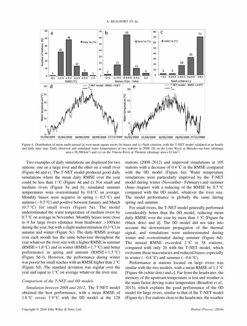
Figure 4. Distribution of mean multi-annual (a) root mean square errors (b) biases and (c) Nash criterion, with the T-NET model validated at an hourlyand daily time step. Daily observed and simulated water temperatures at two stations in 2009: (d) on the Loire River at Muisdes-sur-loire (drainage

area = 38,300 km2) and (e) on the Vincou River at Thouron (drainage area = 81 km2)

A. BEAUFORT ET AL.

Two examples of daily simulations are displayed for twostations: one on a large river and the other on a small river(Figure 4d and e). The T-NET model produced good dailysimulations where the mean daily RMSE over the yearcould be less than 1 °C (Figure 4d and e). For small andmedium rivers (Figure 5a and b), simulated summertemperatures were overestimated by 0.8 °C on average.Monthly biases were negative in spring (�0.5 °C) andautumn (�0.5 °C) and positive between January and March(0.7 °C) for small rivers (Figure 5a). The modelunderestimated the water temperature of medium rivers by0.7 °C on average in November. Monthly biases were closeto 0 for large rivers (distance from headwater >100km)during the year, but with a slight underestimation (0.3 °C) inautumn and winter (Figure 5c). The daily RMSE averageover each month has the same behaviour throughout theyear whatever the river size with a higher RMSE in summer(RMSE=1.8 °C) and in winter (RMSE=1.7 °C) and betterperformance in spring and autumn (RMSE=1.5 °C)(Figure 5d–f). However, the performance during winterwas poorer for small reacheswith anRMSEhigher than 2 °C(Figure 5d). The standard deviation was regular over theyear and equal to 1 °C on average whatever the river size.

Comparison of the T-NET and 0D models

Simulation between 2008 and 2012. The T-NET modelobtained the best performance, with a mean RMSE of1.6 °C versus 1.9 °C with the 0D model at the 128


stations (2008–2012) and improved simulations at 105stations with a decrease of 0.4 °C in the RMSE comparedwith the 0D model (Figure 6a). Water temperaturesimulations were particularly improved by the T-NETmodel during winter (November– February) and summer(June–August) with a reducing of the RMSE by 0.7 °Ccompared with the 0D model, whatever the river size.The model performance is globally the same duringspring and autumn.For small rivers, the T-NET model generally performed

considerably better than the 0D model, reducing meandaily RMSE over the year by more than 1 °C [Figure 6a(black dots) and d]. The 0D model did not take intoaccount the downstream propagation of the thermalsignal, and simulations were underestimated duringwinter and overestimated during summer (Figure 6d).The annual RMSE exceeded 2 °C at 38 stations,compared with only 20 with the T-NET model, whichovercame these inaccuracies and reduced biases, especiallyin winter (�0.8 °C) and summer (�0.6 °C).Performance at stations located on large rivers was

similar with the two models, with a mean RMSE of 1.1 °C[Figure 6b (white dots) and c]. Far from the headwater, thememory of the upstream temperature is lost and weather isthe main factor driving water temperature (Beaufort et al.,2015), which explains the good performance of the 0Dmodel for large rivers, similar to that of the T-NET model(Figure 6c). For stations close to the headwater, the weather


Figure 6. Performance of the T-NET and 0D models: (a) root mean square errors calculated at the 128 monitoring stations between 2008 and 2012 and(b) daily root mean square errors averaged over each month. Daily observed and simulated water temperatures by both models at two stations: (c) on a

large river (drainage area = 38 300 km2) and (d) on a small river (drainage area = 81 km2)

Figure 5. Biases and root mean square errors averaged over each month calculated with the T-NET model between 2008 and 2012 at daily time step atstations (a and d) less than 30 km; (b and e) between 30 and 100 km; and (c and f) more than 100 km from their headwater. Error bars represent 1

standard deviation of values


Copyright © 2016 John Wiley & Sons, Ltd. Hydrol. Process. (2016)

A. BEAUFORT ET AL.

effect is smaller, with greater influence of the headwatertemperature, which may be colder (groundwater insummer, snowmelt) than the local water temperaturedetermined by the 0D model. The T-NET model, whichtakes into account the propagation of the thermal signalfrom upstream to downstream, improved simulations,especially at stations on small and medium rivers that aremore influenced by headwater conditions.

Simulation during flood events in summer 1992 andwinter 2003. The largest summer flood of the Loire(between June and August) since 1984 occurred in 1992.Discharge atDampierre (distance fromheadwater=570km)exceeded 1500m3 s�1 on 14th June, whereas the annualdischarge at this point is 300m3 s�1 (1984–2012). Duringthe flood between 5th June and 10th July, the temperaturedropped by 3 °C at the Dampierre station. The mean dailybiases calculatedwith the T-NET during theflood are 0.2 °C,while the mean biases calculated with the 0D model are2.5 °C. The 0Dmodel obtained amean daily RMSE of 2.5 °Cand failed to simulate the temperature decrease because bydefinition, this model only considers local forcing condi-tions (Figure 7a). The mean daily RMSE calculated with theT-NET model is 0.4 °C because this model takes intoaccount the propagation of the thermal signal from upstreamto downstream and showed excellent capacity to simulatethe cooling of the river during the flood (Figure 7a). Whenthe discharge rises rapidly, the flow velocity increases andthe headwater temperature has more influence because thedownstream travel time is shorter, slowing down theconvergence of the stream temperature and the equilibriumtemperature. During summer, the headwater temperature,considered as the groundwater temperature, is lower thanthe stream temperature by approximately 10°C and has abuffering effect, leading to a drop in the streamtemperature. In December 2003, the largest flood of the

Figure 7. Water temperature of the Loire at Dampierre observed and simulatJune 1992 and (b) the winter flood in December 2003. The second axis


Loire since 1984 was observed, with discharge exceeding3000m3 s�1 on 8th December (Figure 7b). The tempera-ture observed at the Dampierre station decreased by morethan 2 °C during the flood. The T-NET model reproducedthis decrease well with a mean daily bias of 0.2 °C, whilethe 0D model overestimated the water temperature by 1 °Cbecause it did not take into account the influence ofupstream rivers. The T-NET simulated the cooling effectof the flood very accurately.

Simulation of the hot summer of 2003 and the coldsummer of 2002. The summer of 2003 was marked by asevere drought (1 in 50years; rainfall below 10mm inAugust 2003 in the plain area) and a hot spell (maximumdaily Ta>39 °C in August 2003 and mean Ta inAugust = 30 °C), with an increase of 3.2 °C in the meansummer air temperature compared with the 1974–2006summer mean (Bustillo et al., 2014; Moatar andGailhard, 2006). This was an exceptional year becauseclimate projections for the 21st century indicate increas-ing occurrences of hot and dry conditions compared with2003 (Moatar et al., 2010). Water temperatures simulatedby the T-NET model for August 2003 were 0.5 °C colderthan those simulated by the 0D model on average for allrivers located in the Loire basin. The difference oftemperature simulated between both models couldexceed 2 °C for rivers close to their headwater (Figure 8).These cold water streams are located in the upstreammountainous area of the basin where the air is colder (meanair temperature in August 2003=20°C), and also in themiddle sedimentary reaches of the basin where streamsbenefit more from groundwater supplies (Tw<14°C; darkblue Figure 8a) (Beaufort et al., 2015). Temperaturessimulated by the 0Dmodel were influenced more by weatherconditions, which led to a slightly higher simulatedtemperature in the lowland (85% of Tw>25°C with 0D

ed by the T-NET model and the 0D model during (a) the summer flood inrepresents the discharge simulated by the EROS hydrological model


Figure 8. Water temperature simulated by (a) the T-NET model and (b) the 0D model in the Loire basin during the heat wave of August 2003


model vs 80%with T-NETmodel). Simulations on the LoireRiver and its main tributaries were similar with a temperaturehigher than 25°C.The summer of 2002 was colder than 2003 (maximum

daily Ta<28 °C in August 2002 and mean Ta in August23 °C). The performance of the two models for summer2002 was similar, with a median RMSE of 1.7 °C obtainedby the T-NET model and 1.8 °C by the 0D model(Figure 9a). However, the T-NET model performed betterfor the summer of 2003, with an RMSE lower than 1.5 °Cat 49% of stations versus 28% with the 0D model(Figure 9b). RMSE was higher than 3 °C at 18% ofstations with the 0D model versus 3% of stations with theT-NET model. Beaufort et al. (2015) showed that poorlysimulated stations were largely fed by groundwater inputs,which maintained a relatively cool temperature over theentire period under study. The model failed to simulate this

Figure 9. Root mean square errors calculated with the two models at the 47


particularity and underestimated the cooling effect ofgroundwater, which had a stronger influence during theheat wave of 2003, especially on small streams. Converse-ly, the T-NET model was more efficient by taking theupstream influence into account, which improved simula-tions at small and medium rivers close to their headwater.The T-NET model is better at simulating the contrastingresponse of the thermal regime of streams during hot spellsand can offer a better way of studying the thermal responseof rivers to climate change than the 0D model.

Sensitivity analysis of input data

Several input data, including river depth (D), ground-water flow (Qg), shading factor (SF), headwater temper-ature (Tw_head), river width (B), river discharge (Q) andflow velocity (U) remained difficult to quantify at the

stations available in (a) summer 2002 and (b) summer 2003 at a daily time


A. BEAUFORT ET AL.

scale of a large regional watershed. To overcome thesedifficulties, we used a hydrological model to simulate thedaily discharge at 368 subwatershed outlets and empiricalformulae for stream morphological and hydraulic vari-ables as described in the first section of this paper. Here,we will examine the influence of these data on watertemperature simulations at the 128 monitoring stations.Two types of controlling factor can be distinguished:

factors influencing the mean water temperature and thoseinfluencing the water temperature variability.In the first category, we could identify the SF,

headwater temperature (Tw_head) and the groundwaterflow (Qg). The SF had the most influence on the meanwater temperature. At the 128 stations, a 50% variation inSF changed the annual water temperature by ±1.1 °C(Figures 10a and 11b). The major influence of SFoccurred in summer where a variation of ±50% led tomean temperature changes higher than 1.5 °C. Narrowreaches (distance from headwater<30 km) were moresensitive to SF changes (±2 °C) because the canopyshaded the whole reach area. Conversely, the presence ofcanopy along large rivers, such as the Loire (meanwidth=500m), changed the temperature by less than 0.1 °C.The SF is currently considered as constant throughout theyear, which could explain the seasonality of biases for smalland medium rivers in relation with the variation of the solarradiation. One way of improving this would be to take an SFvariable governed by several parameters (vegetation cover,canopy height, position of the sun, river width and season).Recent studies have shown the importance of consideringthe shading variable because this factor can have a stronginfluence on the mean temperature (Moore et al., 2014;Garner et al., 2014).A ±50% variation of the headwater temperature

(Tw_head) leads to a 0.5 °C change in the annual watertemperature. The influence of Tw_head was greater inwinter when the mean temperature changes exceed 0.8 °C

Figure 10. Model sensitivity evaluated at the 128 stations in 2008–2012: (a) dvariability with changes in shading factor (SF), headw


on average, while changes are close to 0 in summer(Figure 10a). The propagation time was shorter in winterand slowed down the speed at which the streamtemperature converges with the equilibrium temperature(Equation 2). In this case, Tw_head plays a major role insimulations and may impact the temperature, even 900kmdownstream (±0.3 °C on the Loire River). Conversely, theinfluence of Tw_head in summer was very limited after100km, and Tw was controlled by weather and localconditions, which explained the good performance of the0D model for large rivers. Stations located on small riversclose to the headwater were the most affected by a changein Tw_head (±1.2 °C), showing the importance of deter-mining the boundary conditions accurately (Tw_head).While the estimation of Tw_head was good (see Section onDatasets), it could be expected that it would also beinfluenced by snowmelt and rainfall. These two factorsare not currently included in the model, suggesting apossible line for improvement.Groundwater flow [m3 s�1] was included in the

streambed input equation to compute the heat budget. Ithad a buffering effect on the thermal regime of rivers, anda 50% increase could reduce the daily variation of watertemperature by 0.3 °C (Figure 11b). The largest temper-ature changes occur at stations located in the central areaof the basin composed of sedimentary rocks, which havea larger groundwater supply. At these stations, the meanwater temperature could rise by 1.1 °C during winter andfall by 1 °C in summer with a groundwater input increaseof 50% (Figure 11b).In the second category of controlling factors, river

discharge was the main factor influencing the watertemperature variability. Discharge is used to calculateflow velocity and was a part of Equation 4 to determine thewater temperature. Discharge has a strong influence onthe daily water temperature variability and is a driver ofthe thermal inertia of the system. A 50% increase in the

istribution of mean river temperature differences and (b) water temperatureater temperature (Tw_head) and river discharge (Q)


Figure 11. Model sensitivity: Distribution of mean river temperature differences and water temperature variability with changes in river depth, groundwaterflow, shading factor, boundary conditions, river width, river discharge and flow velocity of (a)�50% and (b) +50% calculated at the 128 stations in 2008–2012


discharge led to a 0.3 °C rise in the daily water temperatureamplitude (Figure 10b) and had more influence in winter atstations on large rivers (+0.5 °C). Conversely, a decrease inthe discharge led to a reduction in the thermal inertia and a0.3 °C drop in daily temperature amplitude (Figure 10b).River width was also included in Equation 2 anddetermined the exchange area between the river, theatmosphere and the groundwater. The water temperaturetends to converge more quickly to the equilibriumtemperature (Te) if the river is very wide and the dailytemperature variability is high (Figure 11). While thesimulation of the discharge and the calculation of riverwidth and river depth seem to be good (see Section onDatasets), we had few validation measures and some riverscould be poorly simulated. The manner in which thedischarge is distributed within a subwatershed masks thespecific hydrological behaviour of some rivers and couldexplain the poor simulation of local water temperature.One way of improving the simulation of river temperaturewould be to combine the T-NETmodel with a hydrologicalmodel in order to simulate the discharge in each stream.

CONCLUSION

A key issue of this study concerns the improved performanceof thermal simulations by applying the upstream–


downstream propagation of the thermal signal at a regionalscale (110 000km2). The performance level with the T-NETmodel improved at 105 stations, with a 0.4 °C decrease in theRMSE compared with the 0D model. Simulations at stationson small and medium rivers that are more influenced byheadwater conditions were greatly improved, with a decreaseof more than 1°C in the mean RMSE. The T-NET appears tobe considerably better than the 0D model at simulatingspecific events like the floods of June 1992 and the responseof the thermal regime of streams during the heatwave ofAugust 2003. Simulation of the downstream propagation ofthe thermal signal with the T-NET had a mean RMSEof 1.7 °C in summer 2003 versus 2.2 °C with the 0D model.The sensitivity analysis identified the SF and the

headwater temperature as the most influential factors onthe simulated mean water temperature. This factor could bedetermined more accurately by taking into account avariable SF governed by several parameters (vegetationcover, canopy height, sun position, river width and season),which could lead to improved simulations of small andmedium rivers. Another issue raised by this study is thestrong influence of the headwater temperature calculated atthe upstream boundary during winter and autumn. Severalsimulations were tested on the Loire, and water temperaturecan differ by more than 0.5 °C 900km downstream.Conversely, the upstream conditions are more negligible


A. BEAUFORT ET AL.

in summer, particularly 100km from the headwater, whichexplains the good performance of the 0D model on largerivers during summer (Beaufort et al., 2015). Yearsley(2012) has shown the difficulty of simulating the correcttemperature at the upstream boundary and its impact onsimulations further downstream. There is a lack ofvalidation data concerning the measurement of temperatureat the upstream boundary, and to our knowledge, thetemperature of the headwater at the scale of the Loire basinis not monitored, and it was therefore not possible tovalidate. This difficulty could be overcome if we had arepresentative sampling of temperature in the headwaters.The installation of a distributed temperature sensing systemwith an optic fibre cable along the first kilometres from theheadwater could help to better estimate the longitudinalgradient of the stream temperature in the upper reaches(Westhoff et al., 2007). The river discharge is the mainfactor influencing the water temperature variability. Oneway of improving the thermal simulation of river temper-ature would be to combine the T-NET model with ahydrological model in order to simulate the discharge ineach stream at a higher temporal resolution.Finally, this model by propagation offers a good

compromise between performance and transferability. Itcan be easily transposed to changing forcing conditions(physically based structure) in any other catchment.Thermal simulations performed at a daily time step arespatially very consistent at the scale of a hydrographicalreach (~1.7 km). The error structure was convincinglyinterpreted, and based on these results, a regionalizedsimulation of the impact of climate change on the thermalregime of rivers could be achieved.

ACKNOWLEDGEMENTS

This work was realized in the course of work for a thesisfunded by the Office National de l’Eau et des MilieuxAquatiques (ONEMA, National sponsor ID : 18006801701720). It also benefitted from financial supports by theFonds Européen de développement Régional (FEDER,European founds), the Etablissement Public Loire (EPL)and the water Agency of Loire Bretagne (AELB). Thanksare due to Meteo-France for the SAFRAN database, to EDFfor the water temperature data at the station of Dampierreand to Valette et al. for the vegetation database fromIRSTEA. We also thank Yann Jullian and the CaSciModOTfederation (Calcul Scientifique et Modélisation OrléansTours) for their assistance for the implementation of themodel and for the calculations parallelization.

REFERENCES

Beaufort A, Moatar F, Curie F, Ducharne A, Bustillo V, Thiéry D. 2015.River temperature modelling by Strahler order at the regional scale in


the Loire River basin, France. River Research and Applications, inpress. DOI:10.1002/rra.2888

Boyd M, Kasper B. 2003. Analytical methods for dynamic open channelheat and mass transfer: methodology for heat source model, version 7.0,Oregon Dept. of Env. Qual., Portland, Oreg.

Brutsaert W, Stricker H. 1979. An advection–aridity approach to estimateactual regional evapotranspiration.Water Resources Research 15: 443–450.

Buisson L, Blanc L, Grenouillet G. 2008. Modelling stream fish speciesdistribution in a river network: the relative effects of temperature versusphysical factors. Ecology of Freshwater Fish 17(2): 244–257.

Buisson L, Grenouillet G. 2009. Contrasted impacts of climate change onstream fish assemblages along an environmental gradient. Diversity andDistributions 15(4): 613–626.

Bustillo V, Moatar F, Ducharne A, Thiéry D, Poirel A. 2014. Amultimodel comparison for assessing water temperatures underchanging climate conditions via the equilibrium temperature concept:case study of the Middle Loire River, France. Hydrological Processes28: 1507–1524. DOI:10.1002/hyp.9683

Caissie D. 2006. The thermal regime of rivers: a review. FreshwaterBiology 51: 1389–1406.

Carrivick JL, Brown LE, Hannah DM, Turner AGD. 2012. Numericalmodelling of spatio-temporal thermal heterogeneity in a complex riversystem. Journal of Hydrology 414–415: 491–502.

Chapra SC, Pelletier GJ, Tao H. 2008. QUAL2K: a modeling frameworkfor simulating river and stream water quality, version 2.11: documen-tation and users manual, 109 pp., Civil and Environmental EngineeringDept., Tufts Univ., Medford, Mass.

Cole TM, Wells SA. 2002. CE-QUAL-W2: a two-dimensional, laterallyaveraged, hydrodynamic and water quality model, version 3.1, U.S..Army Corps of Engineers Instruction Rep. EL-02-4, 131, pp. +Appendices, U.S. Army Corps of Engineers, Vicksburg, Miss.

Cox MM, Bolte JP. 2007. A spatially explicit network-based model forestimating stream temperature distribution. Environmental Modelling &Software 22: 502–514.

Domisch S, Araujo MB, Bonada N, Pauls SU, Jahnig SC, Haase P. 2013.Modelling distribution in European stream macroinvertebrates underfuture climates. Global Change Biology 19: 752–762. DOI:10.1111/gcb.12107

Edinger JE, Duttweiller D, Geyer J. 1968. The response of watertemperatures to meteorological conditions. Water Resources Research4: 1137–1143.

Edinger JE, Brady DK, Geyer JC. 1974. Heat exchange and transport inthe environment, in Cooling water discharge project (RP- 49), Rep. In14, Electr. Palo Alto, Calif: Power Res. Inst..

Garner G, Hannah DM, Sadler JP, et al. 2013. River temperature regimesof England and Wales: spatial patterns, inter-annual variability andclimatic sensitivity. Hydrological Processes. doi: 10.1002/hyp.9992.

Garner G, Malcolm IA, Sadler JP, Hannah DM. 2014. What causescooling water temperature gradients in forested stream reaches?Hydrology and Earth System Sciences Discussions 11: 6441–6472.DOI:10.5194/hessd-11-6441-2014

Hannah DM, Garner G. 2015. River water temperature in the UnitedKingdom: changes over the 20th century and possible changes over the21st century. Progress in Physical Geography 38: 68–92. DOI:10.1177/0309133314550669

Herb WR, Stefan HG. 2011. Modified equilibrium temperature models forcold-water streams. Water Resources Research 47: W06519. DOI:10.1029/2010WR009586

Kelleher C, Wagener T, Gooseff M, et al. 2012. Investigating controls onthe thermal sensitivity of Pennsylvania streams. Hydrological Processes27: 771–785.

Lamouroux N, Pella H, Vanderbecq A, Sauquet E, Lejot J. 2010.Estimkart 2.0: Une plate-forme de modèles écohydrologiques pourcontribuer à la gestion des cours d’eau à l’échelle des bassins français.Version provisoire. Cemagref – Agence de l’Eau Rhône-Méditerranée-Corse – Onema210.

Lassalle G, Rochard E. 2009. Impact of twenty-first century climatechange on diadromous fish spread over Europe, North Africa and theMiddle East. Global Chang Biol 15: 1072–89.

Loinaz MC, Davidsen HK, Butts M, Bauer-Gottwein P. 2013. Integratedflow and temperature modeling at the catchment scale. Journal ofHydrology 495: 238–251.



Moatar F, Gailhard J. 2006. Water temperature behaviour in the RiverLoire since 1976 and 1881. C.R. Geosciences 338: 319–328.

Moatar F, Ducharne A, Thiéry D, Bustillo V, Sauquet E, Vidal JP.2010. La Loire à l’épreuve du changement climatique. Geosciences12: 78–87. http://www.brgm.fr/dcenewsFile?ID=1306

Mohseni O, Stefan HG. 1999. Stream temperature/air temperature relation-ship: a physical interpretation. Journal of Hydrology 218: 128–141.

Moore RD, Spittlehouse DL, Story A. 2005. Riparian microclimate andstream temperature response to forest harvesting: a review. Journal ofthe American Water Resources Association 41(4): 813–834.

Moore RD, Leach JA, Knudson JM. 2014. Geometric calculation of viewfactors for stream surface radiation modelling in the presence of riparianforest. Hydrological Processes 28: 2975–2986. DOI:10.1002/hyp.9848

O’Driscoll MA, DeWalle DR. 2006. Stream-air temperature relations toclassify stream-ground water interactions in a karst setting, centralPennsylvania, USA. Journal of Hydrology 329: 140–153.

Ouellet V, Secretan Y, St-Hilaire A, Morin J. 2014. Daily averaged 2Dwater temperature model for the St. Lawrence River. River Researchand Applications 30: 733–744. DOI:10.1002/rra.2664

Quintana-Seguí P, Le Moigne P, Durand Y, Martin E, Habets F, BaillonM, Canellas C, Franchisteguy L, Morel S. 2008. Analysis of nearsurface atmospheric variables: validation of the SAFRAN analysis overFrance. J. App. Met. Clim. 47: 92–107. DOI:10.1175/2007JAMC1636.1

Sharma S, Jackson DA, Minns CK, Shuter BJ. 2007. Will northern fishpopulations be in hot water because of climate change? Global ChangeBiology 13: 2052–2064. DOI:10.1111/j.1365-2486.2007.01426.x

Sridhar V, Sansone AL, LaMarche J, Dubin T, Lettenmaier DP. 2004.Prediction of stream temperature in forested watersheds. Journal of theAmerican Water Resources Association 40: 197–211.

Sun N, Yearsley J, Voisin N, Lettenmaier DP. 2014. A spatiallydistributed model for the assessment of land use impacts on streamtemperature in small urban watersheds. Hydrological ProcessesDOI:10.1002/hyp.10363

Thiéry D. 1988. Forecast of changes in piezometric levels by a lumpedhydrological model. Journal of Hydrology 97: 129–148.


Thiéry D, Moutzopoulos C. 1995. Un modèle hydrologique spatialisépour la simulation de très grands bassins: le modèle EROS formé degrappes de modèles globaux élémentaires. In VIIIèmes journéeshydrologiques de l’ORSTOM "Régionalisation en hydrologie, appli-cation au développement", Le Barbé et E (ed). ORSTOM Editions:Servat; 285–295.

Tisseuil C, Vrac M, Grenouillet G, Wade AJ, Gevrey M, Oberdorff T,Grodwohl JB, Lek S. 2012. Strengthening the link between climate,hydrological and species distribution modeling to assess the impacts ofclimate change on freshwater biodiversity. Science of the TotalEnvironment 424: 193–201.

Todd DK. 1980. Groundwater Hydrology. John Wiley: Hoboken, N. J.Valette L, Piffady J, Chandesris A, Souchon Y. 2012. SYRAH-CE:description des données et modélisation du risque d’altération del’hydromorphologie des cours d’eau pour l’Etat des lieux DCE. Rapportfinal, Pôle Hydroécologie des cours d’eau Onema-Irstea Lyon, MALY-LHQ, juillet 2012: 104.

van Vliet MTH, Yearsley JR, Franssen WHP, Ludwig F, Haddeland I,Lettenmaier DP, Kabat P. 2012. Coupled daily streamflow and watertemperature modelling in large river basins. Hydrology and EarthSystem Sciences 16: 4303–4321.

Vidal JP, Martin É, Baillon M, Franchistéguy L, Soubeyroux JM. 2010.A 50-year high-resolution atmospheric reanalysis over France withthe Safran system. International Journal of Climatology 30(11):1627–1644. DOI:10.1002/joc.2003

Westhoff MC, Savenije HHG, Luxemburg WMJ, Stelling GS, vande Giesen NC, Selker JS, Pfister L, Uhlenbrook S. 2007. Adistributed stream temperature model using high resolutiontemperature observations. Hydrology and Earth System Sciences11: 1469–1480.

Yearsley JR. 2009. A semi-Lagrangian water temperature model foradvection-dominated river systems. Water Resources Research 45:W12405 DOI:10.1029/2008WR007629.

Yearsley JR. 2012. A grid-based approach for simulating streamtemperature. Water Resources Research 48: W03506.


http://www.brgm.fr/dcenewsFile?ID=1306

t-net, a dynamic model for simulating daily stream

Documents