T-tests

• Computing a t-test

the t statistic

the t distribution

• Measures of Effect Size

Confidence Intervals

Cohen’s d

Part I

• Computing a t-test

the t statistic

the t distribution

Z as test statistic

n

X

SE

XZ HH

test

00

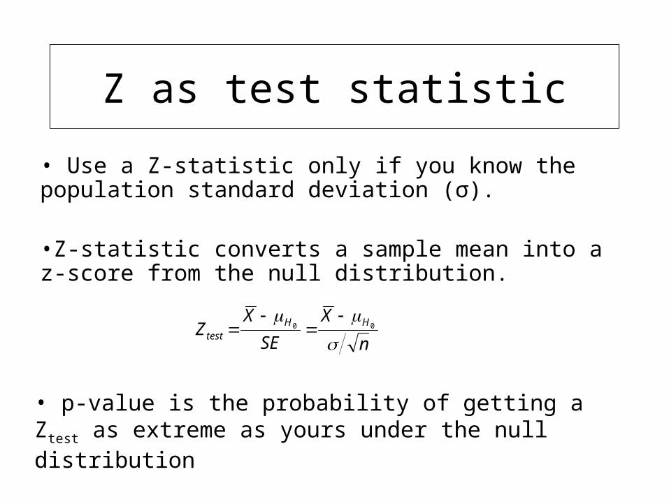
• Use a Z-statistic only if you know the population standard deviation (σ). •Z-statistic converts a sample mean into a z-score from the null distribution.

• p-value is the probability of getting a Ztest as extreme as yours under the null distribution

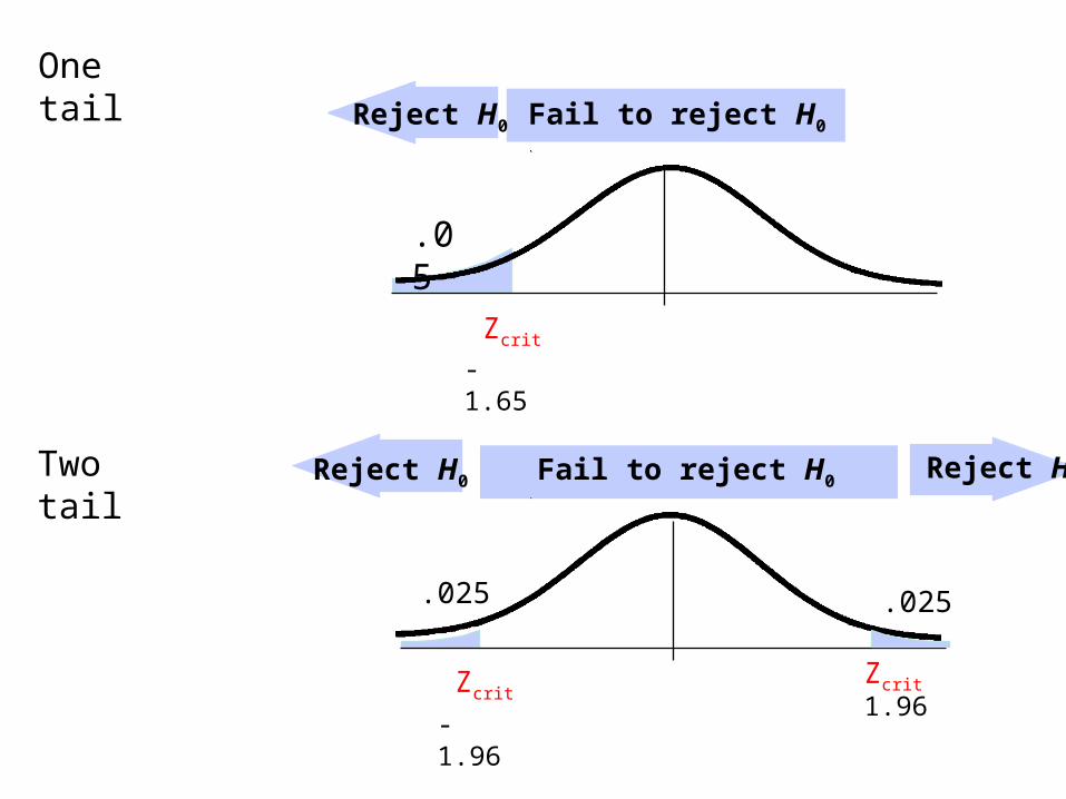
Fail to reject H0Reject H0

One tail

.05

Zcrit

Fail to reject H0Reject H0

.025

Zcrit

Reject H0

Zcrit

-1.961.96

-1.65

.025

Two tail

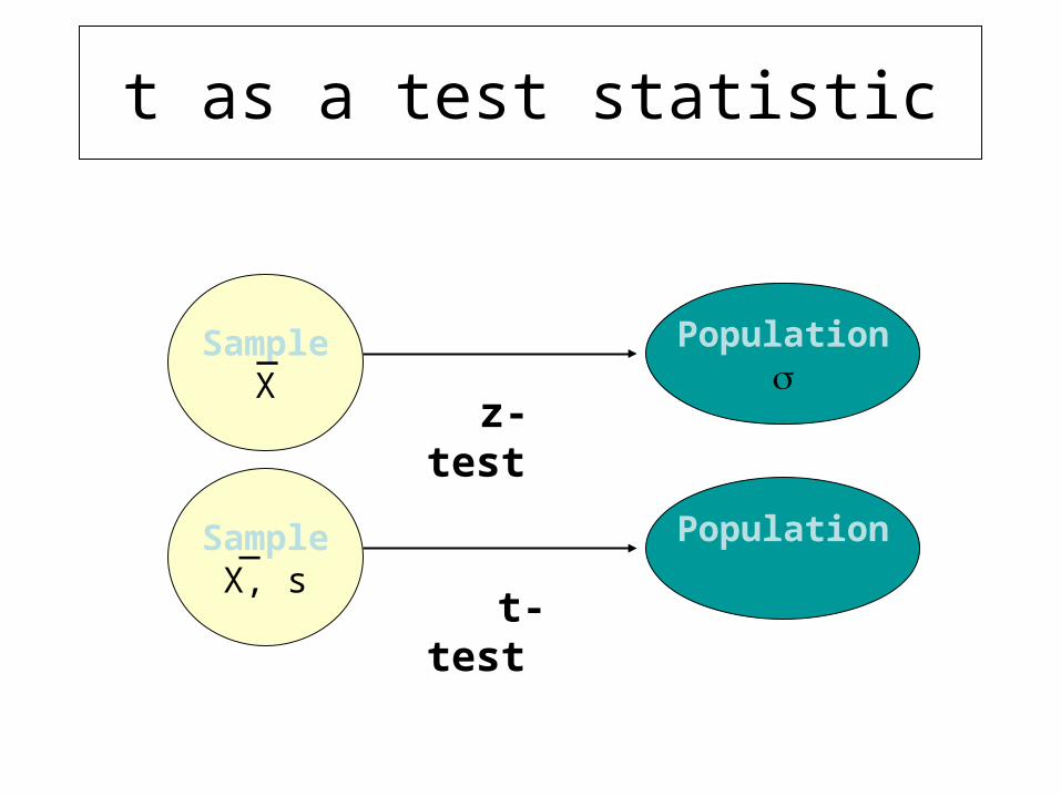
SampleX

z-test

Population

_

SampleX, s

t-test

Population_

t as a test statistic

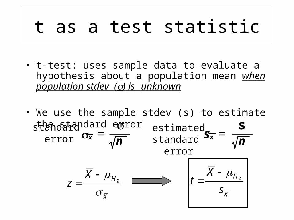
• t-test: uses sample data to evaluate a hypothesis about a population mean when population stdev () is unknown

• We use the sample stdev (s) to estimate the standard error

sx = sn

standard error

estimatedstandard

error

x = n

t as a test statistic

X

H

s

Xt 0

X

HXz

0

t as a test statistic

ns

X

SE

Xt HH

test00

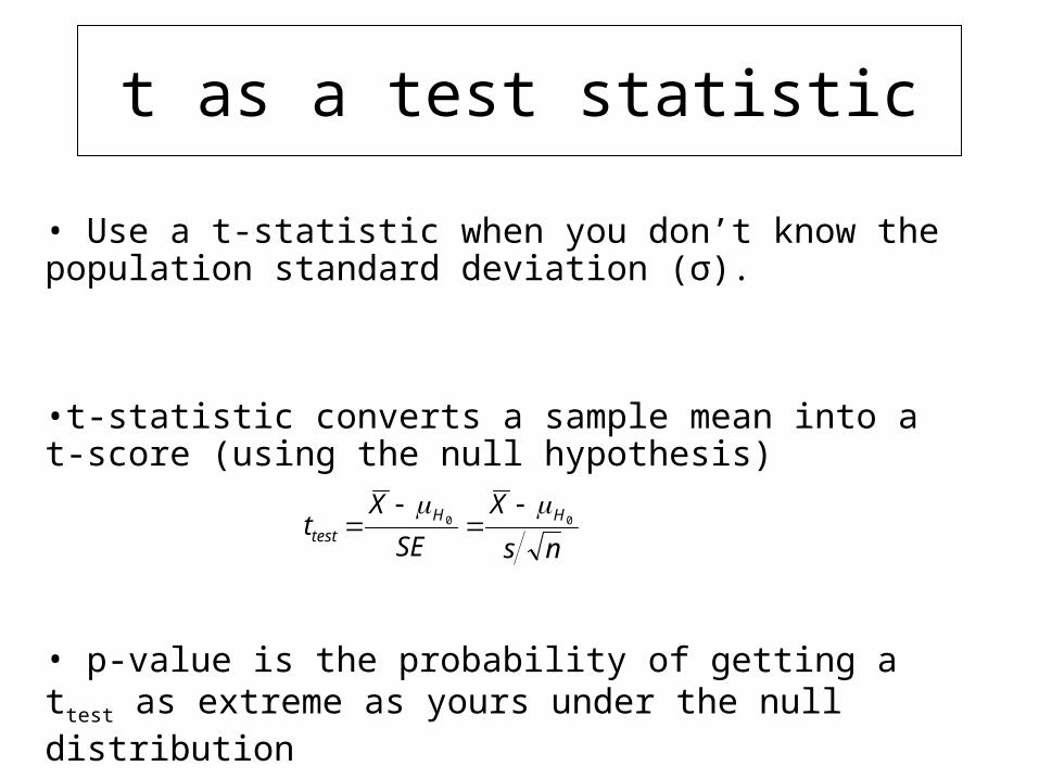
• Use a t-statistic when you don’t know the population standard deviation (σ).

•t-statistic converts a sample mean into a t-score (using the null hypothesis)

• p-value is the probability of getting a ttest as extreme as yours under the null distribution

t distribution

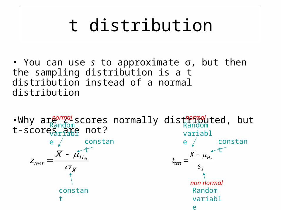
• You can use s to approximate σ, but then the sampling distribution is a t distribution instead of a normal distribution

•Why are Z-scores normally distributed, but t-scores are not?

Random variable

Random variable

constant

X

Htest s

Xt 0

X

Htest

Xz

0

Random variable

constant

constant

normal normal

non normal

t distribution

•With a very large sample, the estimated standard error will be very near the true standard error, and thus t will be almost exactly the same as Z.

•Unlike the standard normal (z) distribution, t is a family of curves. As n gets bigger, t becomes more normal.

•For smaller n, the t distribution is platykurtic (narrower peak, fatter tails)

•We use “degrees of freedom” to identify which t curve to use. For a basic t-test, df = n-1

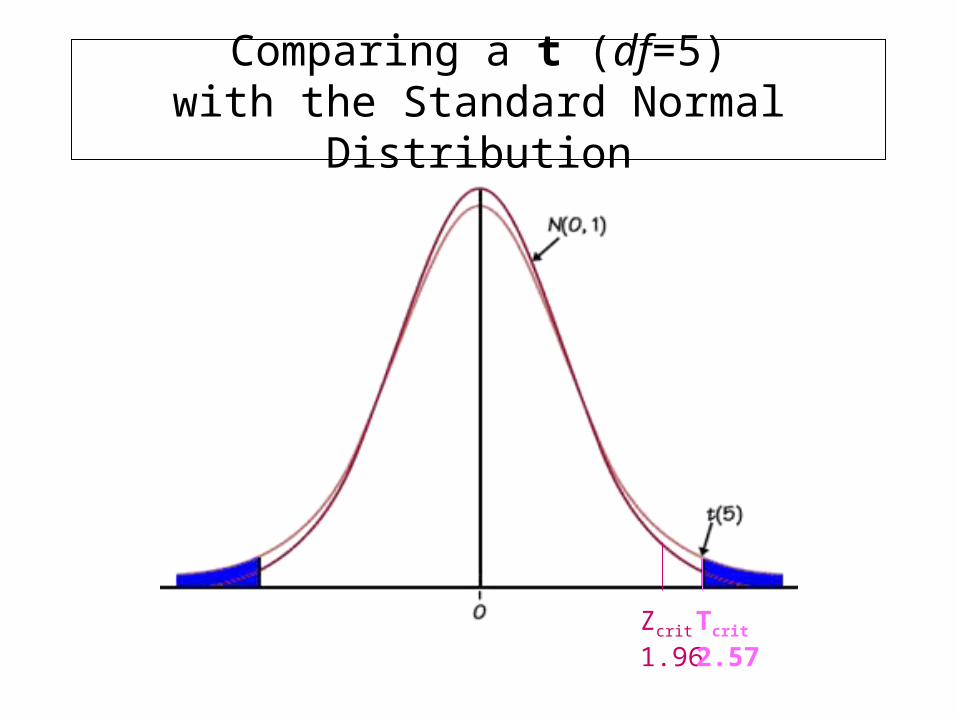
Comparing a t (df=5)with the Standard Normal Distribution

Zcrit

1.96Tcrit2.57

Degrees of freedom

the number of scores in a sample that are free to vary

e.g. for 1 sample, sample mean restricts one value so df = n-1

As df approaches infinity, t-distribution approximates a normal curve

At low df, t-distribution has “fat tails”, which means tcrit is going to be a bit larger than Zcrit. Thus the sample evidence must be more extreme before we get to reject the null. (a tougher test).

t distribution

Too many different curves to put each one in a table. Table E.6 shows just the critical values for one tail at various degrees of freedom and various levels of alpha.

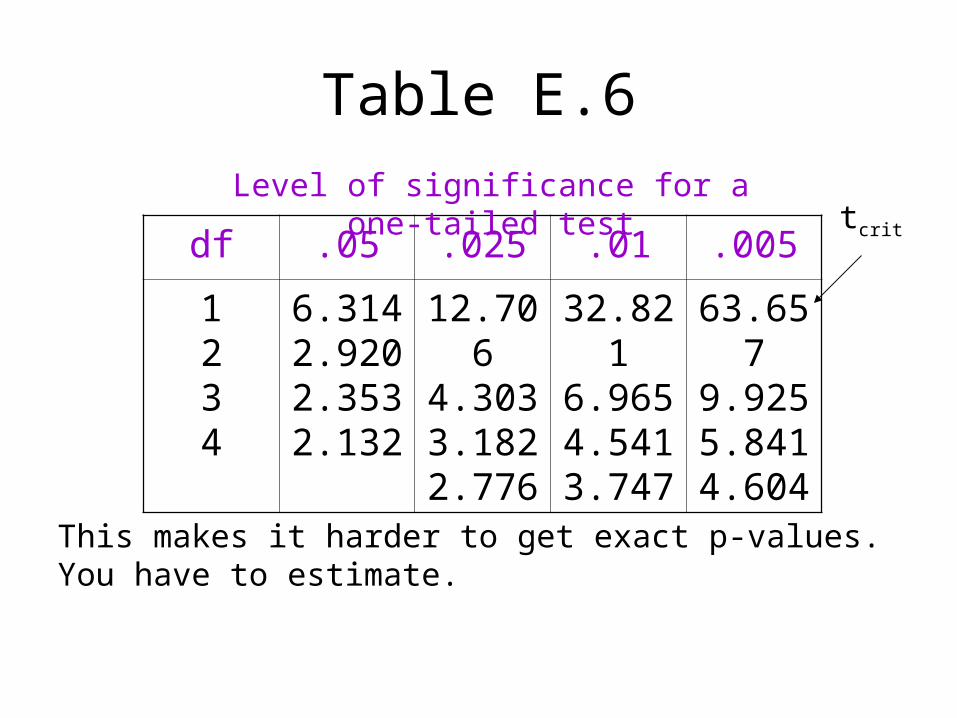
Table E.6

df .05 .025 .01 .005

1234

6.3142.9202.3532.132

12.7064.3033.1822.776

32.8216.9654.5413.747

63.6579.9255.8414.604

Level of significance for a one-tailed testtcrit

This makes it harder to get exact p-values. You have to estimate.

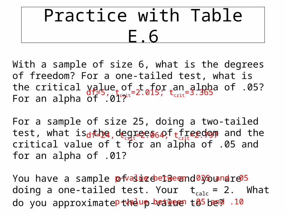
Practice with Table E.6

With a sample of size 6, what is the degrees of freedom? For a one-tailed test, what is the critical value of t for an alpha of .05? For an alpha of .01?

For a sample of size 25, doing a two-tailed test, what is the degrees of freedom and the critical value of t for an alpha of .05 and for an alpha of .01?

You have a sample of size 13 and you are doing a one-tailed test. Your tcalc

= 2. What do you approximate the p-value to be?

What if you had the same data, but were doing a two-tailed test?

df=5, tcrit=2.015; tcrit=3.365

df=24, tcrit=2.064; tcrit=2.797

p-value between .025 and .05

p-value between .05 and .10

Illustration

In a study of families of cancer patients, Compas et al (1994) observed that very young children report few symptoms of anxiety on the CMAS. Contained within the CMAS are nine items that make up a “social desirability scale”. Compas wanted to know if young children have unusually high social desirability scores.

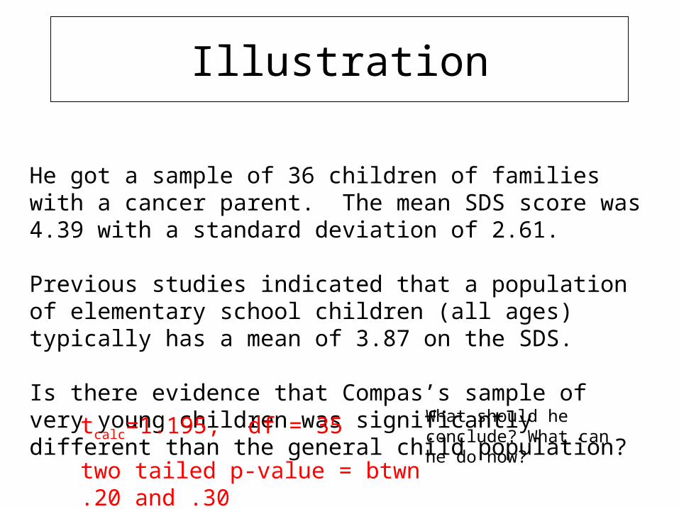
Illustration

He got a sample of 36 children of families with a cancer parent. The mean SDS score was 4.39 with a standard deviation of 2.61.

Previous studies indicated that a population of elementary school children (all ages) typically has a mean of 3.87 on the SDS.

Is there evidence that Compas’s sample of very young children was significantly different than the general child population?

tcalc=1.195, df = 35

two tailed p-value = btwn .20 and .30

What should he conclude? What can he do now?

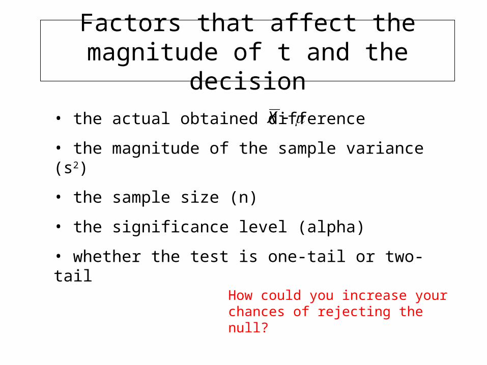
Factors that affect the magnitude of t and the decision

• the actual obtained difference

• the magnitude of the sample variance (s2)

• the sample size (n)

• the significance level (alpha)

• whether the test is one-tail or two-tail

X

How could you increase your chances of rejecting the null?

Part II

• Measures of Effect Size

Confidence Intervals

Cohen’s d

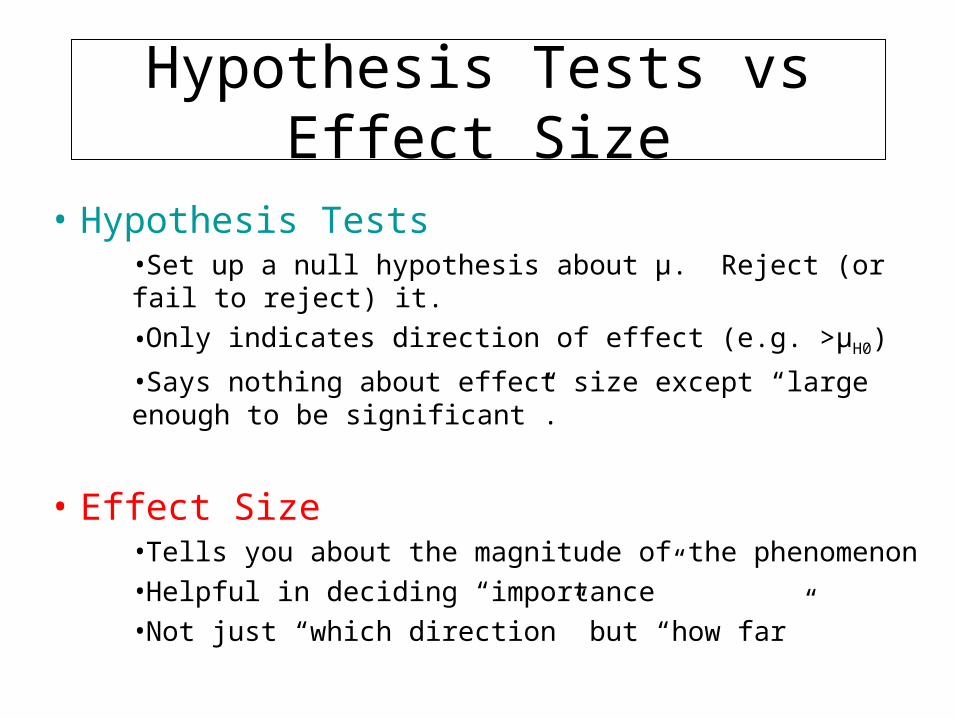
Hypothesis Tests vs Effect Size

• Hypothesis Tests •Set up a null hypothesis about µ. Reject (or fail to reject) it.

•Only indicates direction of effect (e.g. >μH0)

•Says nothing about effect size except “large enough to be significant”.

• Effect Size•Tells you about the magnitude of the phenomenon

•Helpful in deciding “importance”

•Not just “which direction” but “how far”

• “Significant” does not mean important or large

• Significance is dependent on sample size

• “The null hypothesis is never true in fact. Give me a large enough sample and I can guarantee a significant result. ” -Abelson

P-value: Bad Measure of Effect Size

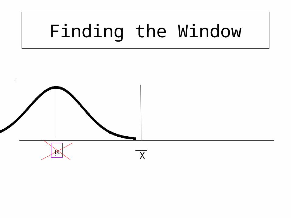
Confidence Interval

• We could estimate effect size with our observed sample deviation

0HX

• But we want a window of uncertainty around that estimate.

• So we provide a “confidence interval” for our observed deviation

• We say we are xx% confident that the true effect size lies somewhere in that window

X__

Finding the Window

X__

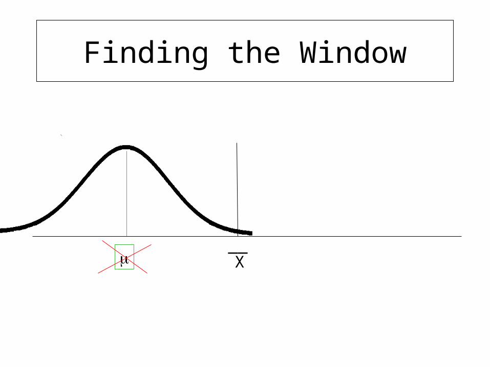
Finding the Window

X__

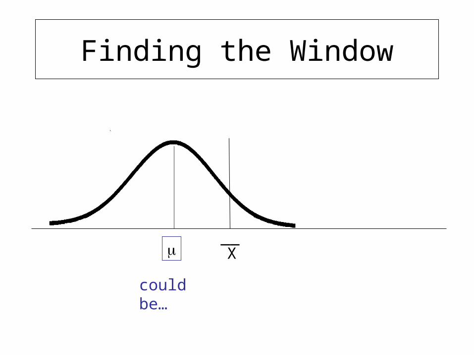
could be…

Finding the Window

X__

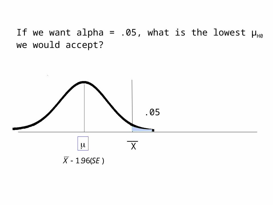
If we want alpha = .05, what is the lowest µH0 we would accept?

.05

)(96.1 SEX

X__

If we want alpha = .05, what is the highest µH0 we would accept?

.05

)(96.1 SEX

X__

)(96.1 SEX )(96.1 SEX

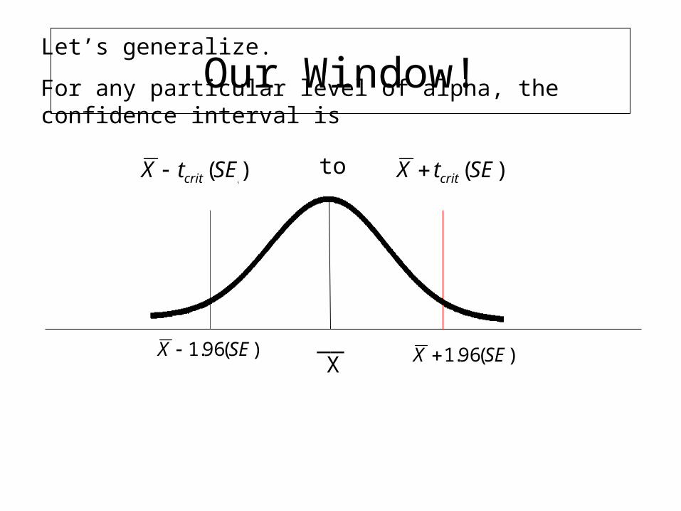
Let’s generalize.

For any particular level of alpha, the confidence interval is

)(SEtX crit )(SEtX critto

Our Window!

Confidence intervals

Confidence level = 1 -

If alpha is .05, then the confidence level is 95%

95% confidence means that 95% of the time, this procedure will capture the true mean (or the true effect) somewhere within the range.

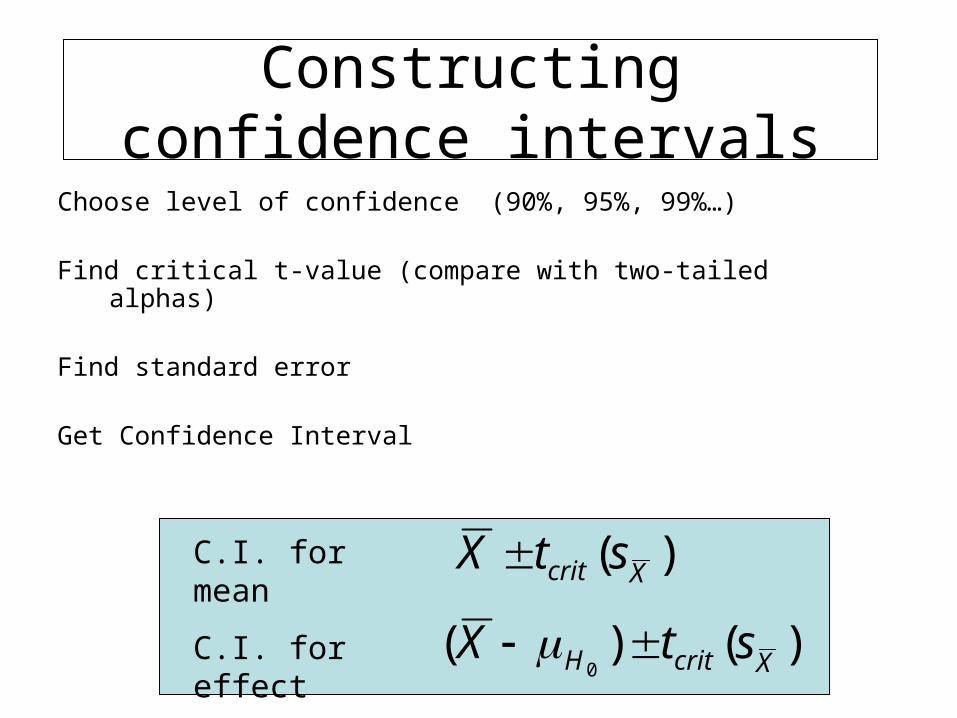
Choose level of confidence (90%, 95%, 99%…)

Find critical t-value (compare with two-tailed alphas)

Find standard error

Get Confidence Interval

Constructing confidence intervals

)( Xcrit stX C.I. for mean

C.I. for effect )()(0 XcritH stX

Exercise in constructing CI

We have a sample of 10 girls who, on average, went on their 1st dates at 15.5 yrs, with a standard deviation of 4.2 years.

What range of values can we assert with 95% confidence contains the true population mean?

Margin = 3 years

CI = (12.50, 18.50) • Using an alpha=.05, would we reject the null hypothesis that µ=10?

•What about that µ=17?

yes

no

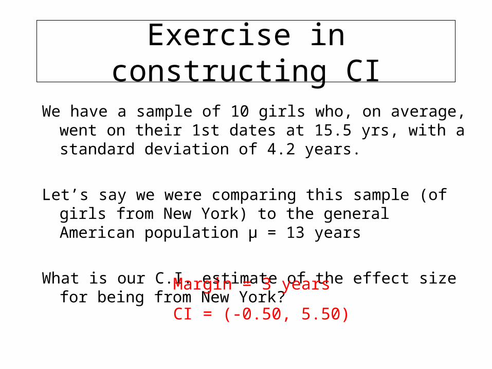
Exercise in constructing CI

We have a sample of 10 girls who, on average, went on their 1st dates at 15.5 yrs, with a standard deviation of 4.2 years.

Let’s say we were comparing this sample (of girls from New York) to the general American population μ = 13 years

What is our C.I. estimate of the effect size for being from New York?

Margin = 3 years

CI = (-0.50, 5.50)

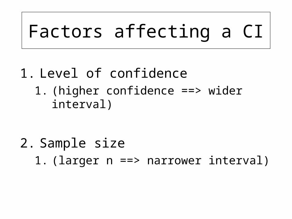
Factors affecting a CI

1. Level of confidence 1. (higher confidence ==> wider interval)

2. Sample size 1. (larger n ==> narrower interval)

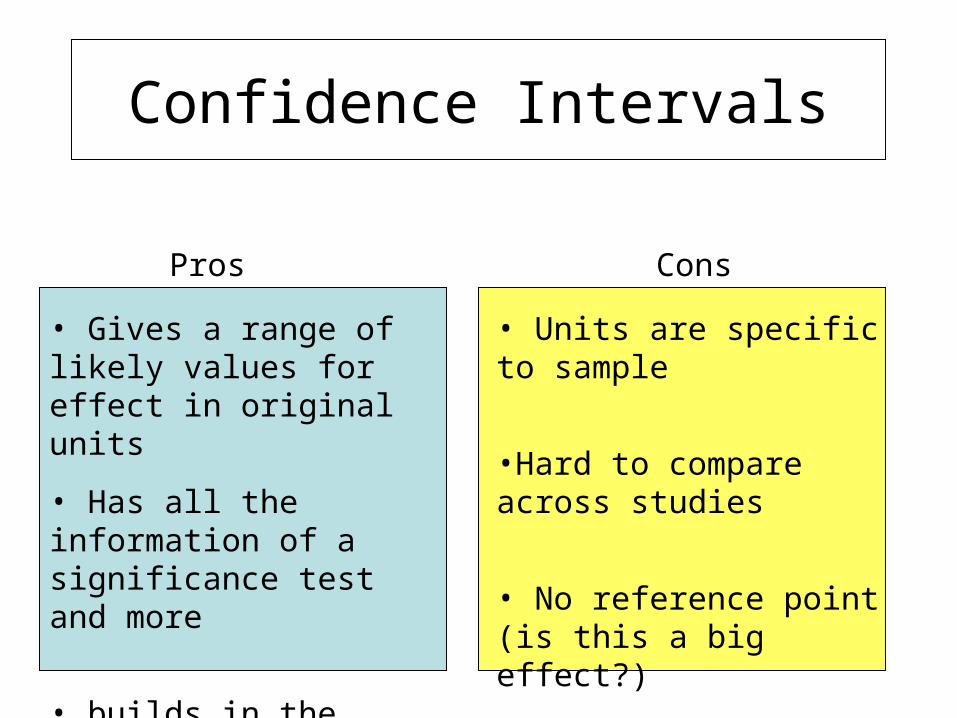
Confidence Intervals

Pros Cons

• Gives a range of likely values for effect in original units

• Has all the information of a significance test and more

• builds in the level of certainty

• Units are specific to sample

•Hard to compare across studies

• No reference point (is this a big effect?)

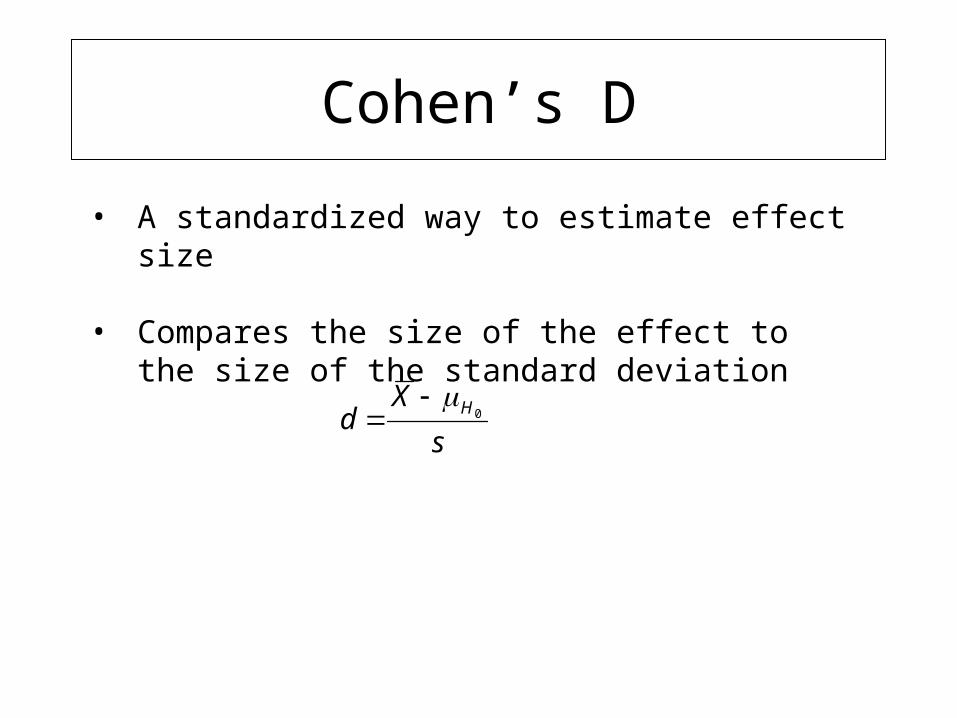
Cohen’s D

s

Xd H0

• A standardized way to estimate effect size

• Compares the size of the effect to the size of the standard deviation

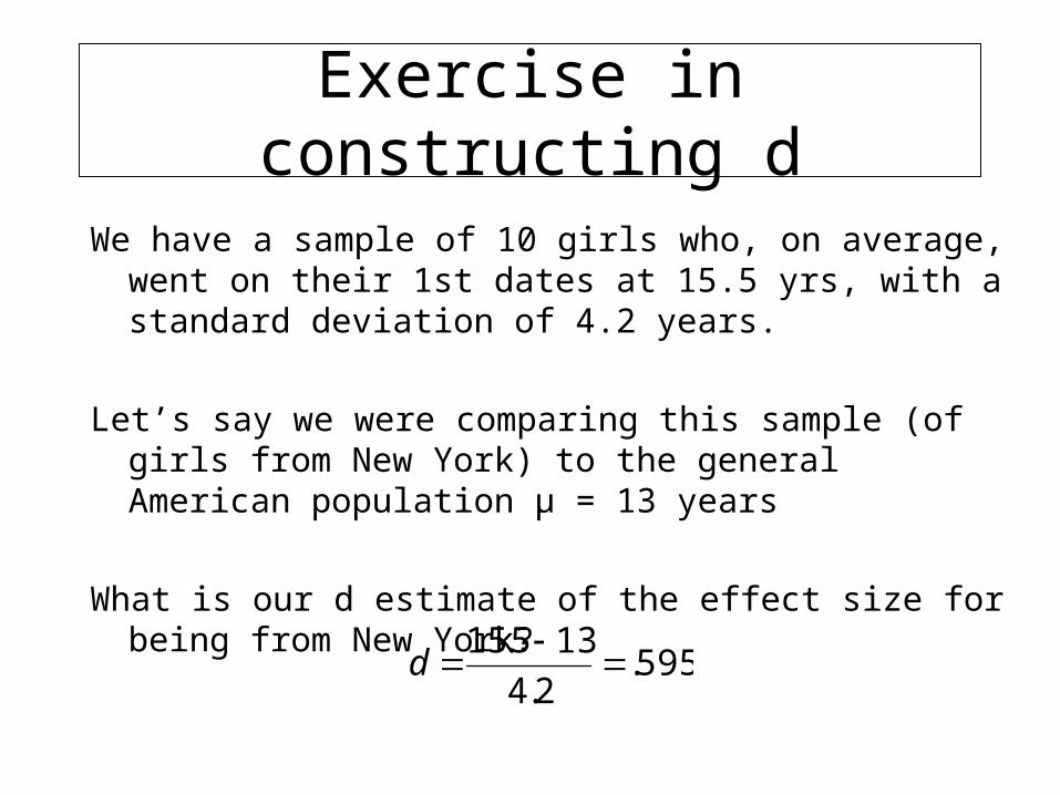
Exercise in constructing d

We have a sample of 10 girls who, on average, went on their 1st dates at 15.5 yrs, with a standard deviation of 4.2 years.

Let’s say we were comparing this sample (of girls from New York) to the general American population μ = 13 years

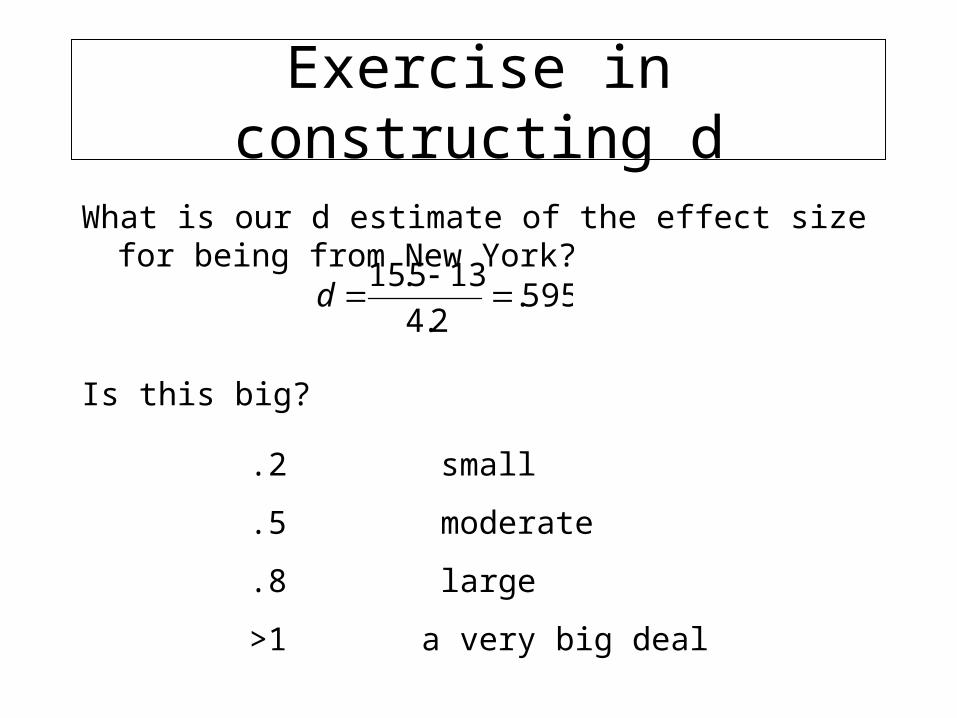
What is our d estimate of the effect size for being from New York?

595.2.4

135.15

d

Exercise in constructing d

What is our d estimate of the effect size for being from New York?

Is this big?

595.2.4

135.15

d

.2 small

.5 moderate

.8 large

>1 a very big deal

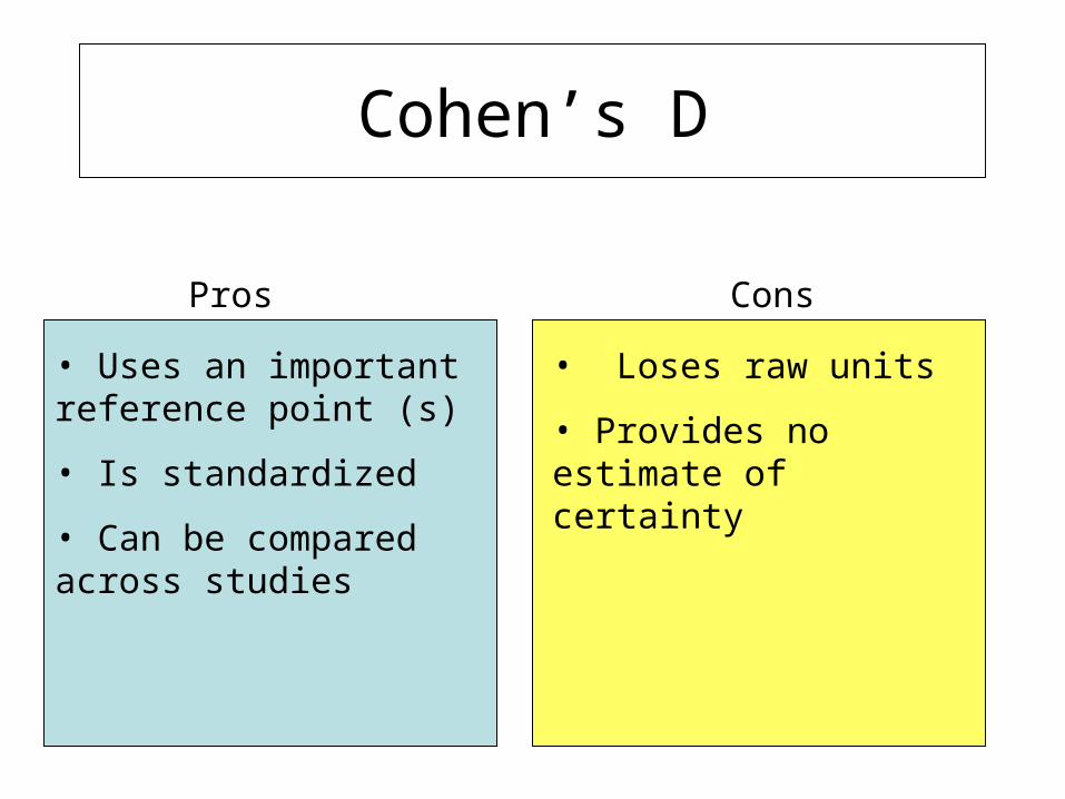
Cohen’s D

Pros Cons

• Uses an important reference point (s)

• Is standardized

• Can be compared across studies

• Loses raw units

• Provides no estimate of certainty

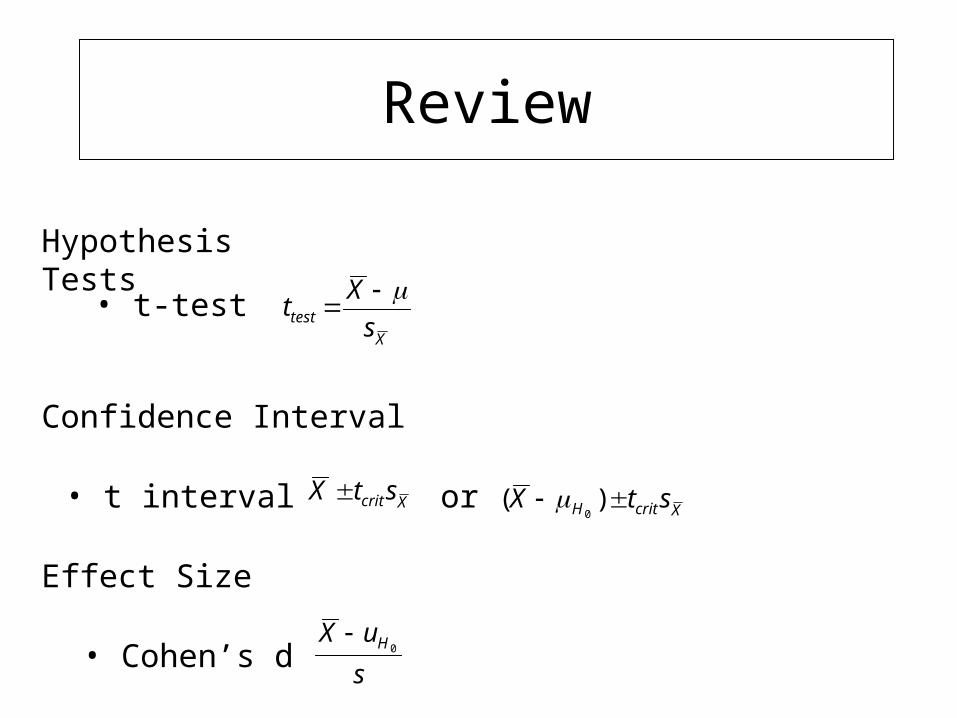
Review

Hypothesis Tests

Confidence Interval

• t-testX

test s

Xt

• t interval Xcrit stX

Effect Size

• Cohen’s ds

uX H0

XcritH stX )(0

or