T5 C13 Integral Calculus Overview

Calculus consists of two concepts, Derivative and Integral.

We have already studied the Derivative, or Differential Calculus.

Now we will study the Integral, or Integral Calculus.

What kind of problems will Integral Calculus address?

What we might call “accumulation” problems.

For example, the Area of a two dimensional object, or the Volume or Surface Area of a three dimensional object.

Our pre-calculus ancestors were able to calculate the areas and volumes of some common geometric objects, which we studied in Geometry in Tiers 2, 3, and 4. But, these studies were limited to some very special cases.

In STEM subjects we must be able to calculate areas and volumes of a much broader class of objects.

Example 1, What would be the area under a parabola in the figure below? Or of an ellipse?

Archimedes figured out the parabola. Can you?

What about the ellipse?

Example 2. What about the area under a circle bounded by two vertical lines from a diameter? (You draw it)

Example 3. What about the area under the sine curve?

Example 4. What about the volume or surface area of a paraboloid, i.e. a surface where a parabola is rotated about its axis. This is how many “dish” receivers are made.

Example 5. What about the arc length of a curve?

Many of these examples are easily solved with integral calculus. How?

An irony is that one key to their solution is to use what are called anti-derivatives, which of course we get from derivatives. This is what our ancestors discovered and used for three hundred years.

Indeed, this discovery is called the Fundamental Theorem of Calculus, and one can argue that all of modern technology grew from this discovery.

All that changed with the invention of a computer. Now, if you have access to a computer you can get very accurate estimates by brute force using a computer.

Ironically, today with a tool like WA you can solve these problems both ways as you will learn.

First, you will learn the definition of “Integral” from a geometric viewpoint.

Second, you will learn how to use the Fundamental Theorem of Calculus like our ancestors did and then to utilize WA to evaluate any integral.

Finally, you will learn how WA can calculate the value of any integral to a high degree of accuracy by brute force that would be impractical for a human to do manually, even with a calculator.

Today it is pretty easy to learn the basic calculus concepts and how to use a tool like Wolfram Alpha to solve any calculus problem.

There are many applications of integrals in virtually all subjects in science and engineering and any other quantitative field.

If you go into a STEM field you will be finding examples in a never ending way. There are an unlimited number of examples.

Many of the integral calculus tools our ancestors developed and used are now effectively obsolete in that no employer would pay you to use these “manual tools” to solve a calculus problem.

These tools are still taught in typical calculus courses and covered in typical calculus textbooks. You may learn them if you like. And then, you may always check your work easily and quickly with Wolfram Alpha.

A modern calculus textbook will be a good source of problems and applications of both differential and integral calculus.

You may solve the problems with the classical manual techniques if you like or simply use Wolfram Alpha.

It is imperative you learn to use a tool like Wolfram Alpha since this is what any modern STEM professional uses.

Wolfram Alpha makes the application of calculus 90% easier than the old classical approach.

This, in turn, makes it easier to understand the concepts of calculus and their applications.

T5 C13 Integral Calculus Overview Homework

Q1. What kind of problems does integral calculus address?

Q2. Name two types of problems integral calculus can help with?

Q3. Integrals are also called what?

Q4. What does the Fundamental Theorem of Calculus do?

A1. Accumulation problems

A2. The area of a two dimensional object, or the volume or surface area of a three dimensional object.

A3. Anti-derivatives

A4. It links the concept of the derivative of a function with the concept of the integral of a function.

T5 C14 Definition of Integral and the FTC.

Definition of Integral.

Let y = f(t) be a continuous function and a < x

F(x) = the area under the graph of f from a to x.

Notation: F(x) =

Fundamental Theorem of Calculus (FTC) I.

F’(x) = f(x)

F is called an anti-derivative of f.

Corollary: The area under the graph of the function f from a to b for a < b is F(b)

Area under f from a to b = F(b) =

Demo of FTC

Let h be an infinitesmal

F(x + h) – F(x) ≈ f(x)h

(F(x + h) – F(x))/h ≈ f(x)

F’(x) = Std[(F(x + h) – F(x))/h] = f(x)

This Demo can be made quite rigorous.

Why is this important?

Lemma 1. If for all x, H(x) = C, the H’(x) = 0 for all x.

Proof: H’(x) = std{[H(x+h) – H(x)]/h}=std[0/h] = 0

Lemma 2. If H(x) is continuous and H’(x) = 0 for all x, then H(x) = C for some constant C.

Proof: This can be proven rigorously, but heuristically we see the Graph of H is flat for all x and thus it can never increase or decrease for any x and , thus it is always constant for some number C.

Lemma 3. If F’(x) = G’(x) = f(x) for all x, then

F(x) = G(x) + C, for some constant C, for all x.

Proof: (F – G)’(x) = F’(x) – G’(x) = 0

Thus, (F – G)(x) = C for some constant C,

Thus F(x) – G(x) = C or F(x) = G(x) + C

What is the significance of these three Lemmas?

Well suppose we somehow can find an antiderivative G of the function f. G’(x) = f(x)

From Lemma 3 we now know that F(x) = G(x) + C for some constant C.

We also know that 0 = F(a) = G(a) +C, or C = -G(a)

So we now get

Fundamental Theorem of Calculus (FTC II)

Area under y = f(t) from a to b = G(b) – G(a)

So this means that if we can somehow find an antiderivative F(t) of f(t) then we can calculate the area under the graph of f from a to b by just evaluating this antiderivative at a and b and substracting.

Sometimes finding an antiderivative F(t) for f(t) is easy. Certainly, if we know F’(t) = f(t) for some F, the F is the antiderivative of f.

So for example -cos(t) is the antiderivative of sin(t) since we know the derivative of -cos(t) is sin(t).

Unfortunately, finding an antiderivative for many functions f(t) is very difficult, and sometimes impossible in terms of any familiar functions.

Finding these antiderivatives is part of what is called “techniques of integration”, and it the reason Integral Calculus has classically been so difficult.

Fortunately, WA will find these antiderivatives for you in virtually all cases.

WA antiderivative sin(x) Answer: -cos(x) + C

WA derivative –cos(x) Of course

Notice: an antiderivative F(x) of a function f(x) is also called an indefinite integral of f(x).

WA integrate sin(x)

WA indefinite integral sin(x)

WA integrate sin(x) from x = 1 to 3

Also gives you the definite integral from 1 to 3, and thus the net area under the graph of sin(x).

Example 1: We know the derivative of -cos(x) is sin(x)

or an antiderivative of sin(x) is –cos(x)

So we can calculate the area under the sine curve from

.1 to 1.45 as –cos(1.45) – (-cos(.1) = .874501

Of course, WA gives this quickly too.

WA Integrate sin(x) from .1 to 1.45

Example 2: We know that the derivative of (1/3)x3 = x

So an antiderivative of x

2

2 = (1/3)x3

So the area under the parabola x

is

2

(1/3)3.2

from x = 1.5 to 3.2 is

3 - (1/3)1.53

Check with WA.

= 9.79767

WA Integrate x^2 from x = 1.5 to 3.2

Example 3 Find the area under the upper semicircle of radius 5 centered at the origin from x = -2 to 2

The equation of the circle is x^2 + y^2 = 25

So, y = (25 – x2)1/2

So all we have to do is find an anti-derivative of this function and apply the FTC!

is the function whose graph is the upper semicircle.

Oops!. Easier said, than done. Do you know one?

Can you find one? Pause and try it.

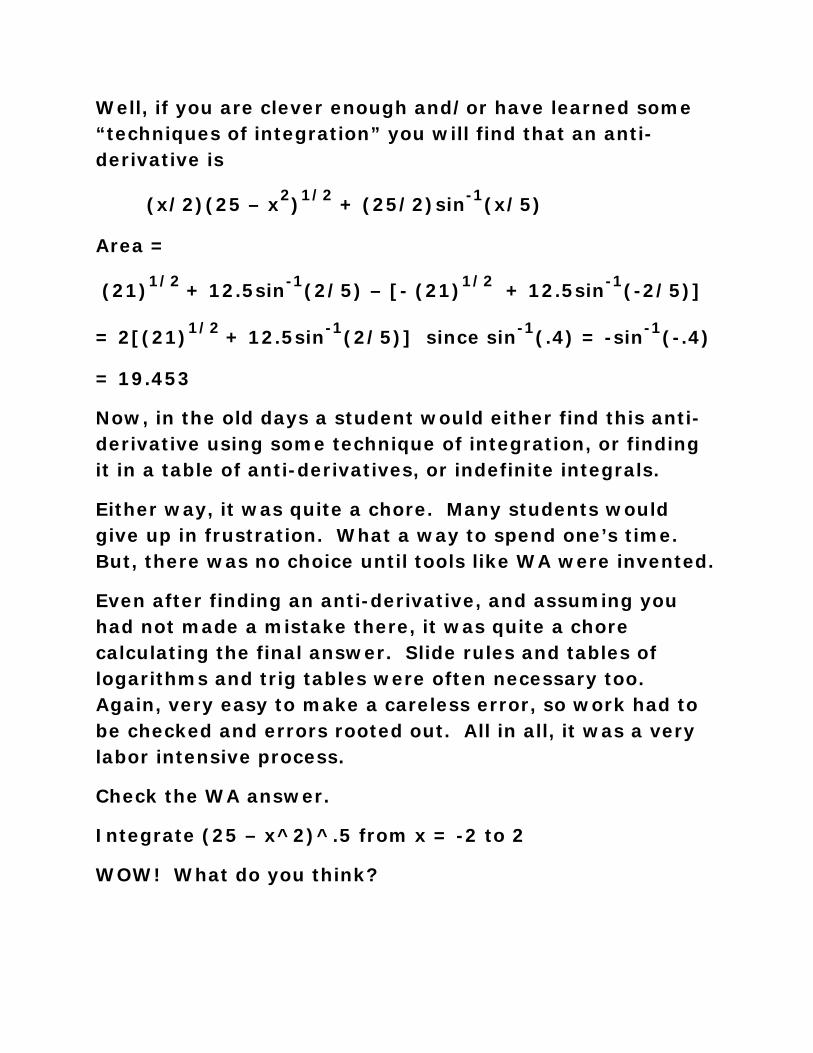
Well, if you are clever enough and/or have learned some “techniques of integration” you will find that an anti-derivative is

(x/2)(25 – x2)1/2 + (25/2)sin-1

Area =

(x/5)

(21)1/2 + 12.5sin-1(2/5) – [- (21)1/2 + 12.5sin-1

= 2[(21)

(-2/5)]

1/2 + 12.5sin-1(2/5)] since sin-1(.4) = -sin-1

= 19.453

(-.4)

Now, in the old days a student would either find this anti-derivative using some technique of integration, or finding it in a table of anti-derivatives, or indefinite integrals.

Either way, it was quite a chore. Many students would give up in frustration. What a way to spend one’s time. But, there was no choice until tools like WA were invented.

Even after finding an anti-derivative, and assuming you had not made a mistake there, it was quite a chore calculating the final answer. Slide rules and tables of logarithms and trig tables were often necessary too. Again, very easy to make a careless error, so work had to be checked and errors rooted out. All in all, it was a very labor intensive process.

Check the WA answer.

Integrate (25 – x^2)^.5 from x = -2 to 2

WOW! What do you think?

T5 C14 Definition of Integral and the FTC Exercises

Q1. If you are given a function f(x), and F(x) is defined to be the area under the graph of f(t) from t = a to t = x, then what is F(x) called?

Q2. What is Part I of the Fundamental Theorem of Calculus (FTC)?

Q3. If you are given a function f(x), graphed from a to b, what is the notation for the area under the graph using the definition of F(x) from Q1?

Q4. An anti-derivative is also called what, and why?

Q5. What is a definite integral?

Q6. Given the function f(x) = cos(2x)2

Q7. Given the function f(x) = 1/3(2x

, what is the anti-derivative and what is the area from x = 0.2 to 0.4?

2 -3x)2

Note: When you just find the antiderivative or indefinite integral of f(x), then Wolfram Alpha also gives you its graph and not the graph of f(x).

, what is the anti-derivative and what is the area from x = 0.5 to 1.4?

But, when you find the definite integral of f(x) Wolfram Alpha now gives you the graph of f(x) from a to b and not the graph of F(x) the antiderivative.

Q8. Given the function f(x) = -sin(x) -3x3

Q9. Given the function f(x) = cos(2x)

, what is the area from x = 0 to 1.75?

3

Q10. Find the area under the upper semicircle of radius 7 centered at the origin from x = -3 to 3. The function whose graph is the upper semi-circle is f(x) = (49 – x

, what is the area from x = 0 to π/2 ?

2)1/2

.

A1. The integral of f(t) from t = a to t = x, and also by the FTC if is an anti-derivative of f(x).

A2. F’(x) = f(x)

A3. F(b) or F(b) – F(a) But, of course, F(a) = 0

A4. An indefinite integral, because it has no upper or lower limits

A5. An integral that has upper and lower limits

A6. WA integrate cos(2x)^2

WA integrate cos(2x)^2 from x = 0.2 to 0.4

Area = 0.135277

A7. WA integrate 1/3(2x^2 -3x)^2

WA integrate 1/3(2x^2 -3x)^2 from x = 0.5 to 1.4

Area = 0.265764

A8. WA integrate -sin(x) -3x^3

WA integrate -sin(x) -3x^3 from x = 0 to 1.75

Area = -8.21243

A9. WA integrate cos(2x)^3

WA integrate cos(2x)^3 from x = 0 to pi/2

Area=0

A10. WA integrate (49 – x^2)^(1/2)

WA integrate (49 – x^2)^(1/2) from x = -3 to 3

Area=40.676

T5 C15 Techniques of Integration

An indefinite integral F(x) = ∫f(x)dx is an anti-derivative of f(x).

A definite integral of f(x) from a to b is F(b)–F(a).

How to calculate this definite integral is the question.

I. Brute Force

Conceptually, an integral is very simple geometrically and arithmetically.

It is simply the sum of a bunch of rectangles to be summed up. f(x)dx indicates this in the integral notation. f(x) is the length and dx is the width. Add them all up!

Divide (a,b) into n equal sub-intervals

a =a0, a1, a2, a3,. . ., an

The length of each subinterval is

= b

(b – a)/n = ∆n

Calculate f(ai

Integral of f(x) from a to b

+ ∆n/2) for each i = 0 to n-1

≈ Sum[f(ai

Now it’s just an arithmetic problem.

+ ∆n/2) ∆n] i = 0,…,n-1

The larger n, the more accurate the value.

Remember, in any practical STEM calculation, there is always an error term.

This method was quite impractical for our ancestors, with just pencil and paper, even with logarithms, trig tables, and slide rules.

It simply took too long and was error prone and required many redundant calculations to check.

But, with a computer, this is a trivial calculation.

So, up until about 50 years ago, our ancestors had to rely on other techniques.

II. Use the Fundamental Theorem of Calculus

This is easy IF you can find an anti-derivative for f(x)

Otherwise, the FTC doesn’t help.

Well, taking derivatives is pretty easy and algorithmic. So our ancestors made up very elaborate tables of derivatives.

Then working the tables backward one had anti-derivatives. These were called tables of (indefinite) integrals. They were extensive and compiled with an immense amount of labor by many mathematicians over many decades, even centuries.

After all, the FTC was discovered in the 1600’s. It was the “open sesame” to calculating definite integrals, which one must do for virtually all STEM subjects.

The FTC spawned the industrial revolution. Modern civilization is based on it.

Mathematicians like Euler and many others compiled very extensive tables of integrals. In fact, it was still quite challenging to find a desired anti-derivative in these extensive tables. But, it was often the only practical way to find an anti-derivative.

Calculus books were written to take full advantage of the FTC for evaluating integrals.

Many “techniques of integration” were devised to find these anti-derivatives. These were a collection of ad-hoc techniques that were difficult to master and remember.

One would need to spend a great deal of time learning and practicing these techniques to become even marginally proficient.

These techniques were responsible for many students giving up on learning math and abandoning a STEM career.

And, worse yet, there were many functions that simply did not have anti-derivatives represented by the common functions everyone understood.

This led to the definitions of many new Special Functions, whose definitions were essentially given by the integrals of certain functions.

Example: What is the anti-derivative of sin(x2

It is easy to find an anti-derivative of xsin(x

)?

2) using the

techniques taught in a calculus textbook. It is -.5cos(x2

So this could be put on a test for calculus.

)

But, try as hard as you like NONE of the techniques of integration taught in any calculus textbook will yield an anti-derivative for sin(x2

In fact, this anti-derivative is given a name, it is the Special Function called a Fresnal Integral. There are then tables of values for this Fresnal Integral, so you can evaluate the integral of sin(x

).

2

WA integrate xsin(x^2) WA Integrate sin(x^2)

)!

WA Plot sin(x^2) WA integrate sin(x^2) from -1 to 1

Our calculus textbooks were developed in the late 1800’s and evolved throughout the 20th

In addition to these techniques of integration, in the 20

century.

th

Many engineers and scientists, and non-mathematicians, would skip the rigor, but they could not escape the techniques of integration using anti-derivatives and the FTC. There simply wasn’t a better way.

Century, calculus textbook authors felt a necessity to introduce rigorous arguments and “proofs” into these calculus textbooks too. This made the learning of calculus even more difficult for most students.

There were extensive tables of antiderivatives or indefinite integrals compiled that made it somewhat easier to find antiderivatives. But, even these could be challenging to use. You often had to transform a function of interest into another form to find your antiderivative.

There was simply no easy way to find antiderivatives for real world functions. Thus, integration was difficult.

III. Use a polynomial approximation or infinite series representation of a function.

Then one could easily find an anti-derivative since it is very easy, for anyone, to find the anti-derivative of a polynomial.

Furthermore, it is possible to find such a representation of virtually any function using what is called a Taylor Series expansion of the function. But, this is time consuming, and sometimes very difficult too.

Our early ancestors utilized the generalized Binomial Theorem to obtain a polynomial representation of many functions. Isaac Newton was very adept at this.

However, it turns out that it is also a very burdensome arithmetical challenge to utilize this infinite series approach too. It sometimes isn’t much easier that the Brute Force Method.

Once computers became available to engineers and scientists method I., Brute Force, became very popular.

Today, (circa 2015) we have the best of both worlds thanks to Wolfram Alpha.

WA will give you the antiderivative of virtually any function, if one exists. And, then you can use this to find the definite integral. Otherwise, it simply utilizes Brute Force to calculate a definite integral. In fact, it does it all with one simple command.

Integrate f(x) from x= a to b.

No modern employer is going to pay an employee to use antiquated methods for finding integrals. It is simply too time consuming and error prone, and in many cases virtually impossible.

It would be like expecting a modern STEM professional to use a slide-rule, or log tables, or trig tables, to solve problems.

It’s like making a student use manual algorithms and pencil and paper to do arithmetical calculations instead of using a calculator.

You need to learn to use a modern tool like Wolfram Alpha to solve such problems.

This results in a huge improvement in both Quality and Productivity.

If you are going to study a STEM subject in some school, I would ask if they will allow you to use modern tools like WA to solve calculus problems, and differential equations, and linear algebra, and many other types of math problems.

If they insist you learn antiquated, difficult, and irrelevant techniques, I would choose another school.

Unfortunately, some math departments are still mired in the old ways and might want to insist you master useless outdated techniques.

After all, teachers like to teach what they know and learned with great effort.

And, they are often forced to do so by the choice of textbooks and syllabi forced on them by their schools.

It will be your decision whether you want to comply.

Personally, I would not want to waste my valuable time and money in such a school.

At the end of this course, I will teach you a few of the tools for techniques of integration, as a historical curiosity, and perhaps help you pass some antiquated test.

T5 C15 Techniques of Integration Exercises

Q1. Given that the definite integral of f(x) from a to b is F(b)–F(a), what is the general form for calculating the area from a to b using the Brute Force method?

Q2. In the answer to Q1, what does the term ∆n represent mathematically?

Q3. In the answer to Q3, what does n represent, and which will give you a more accurate value for your area estimation, a larger or smaller value for n?

For the following exercises, plot the function, then find the definite integral for the range given.

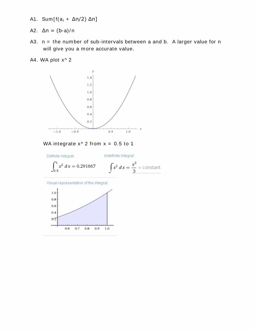
Q4. f(x) = x2

Q5. f(x) = 4x

range: 0.5 to 1.0

3 - x2

Q6. f(x) = cos(x

range: 0.1 to 0.2

2

Q7. f(x) = sin(x

) + sin(x) range: 0 to 3

2

Q8. f(x) = 4e

) - cos(x) range: -2 to 2

x^3

Q9. f(x) = ln(5x

range: 0.5 to 1.0

2

Q10. f(x) = e

+ sin(x)) range: -4 to -2

x

range: -3 to 0

A1. Sum[f(ai

A2. ∆n = (b-a)/n

+ ∆n/2) ∆n]

A3. n = the number of sub-intervals between a and b. A larger value for n will give you a more accurate value.

A4. WA plot x^2

WA integrate x^2 from x = 0.5 to 1

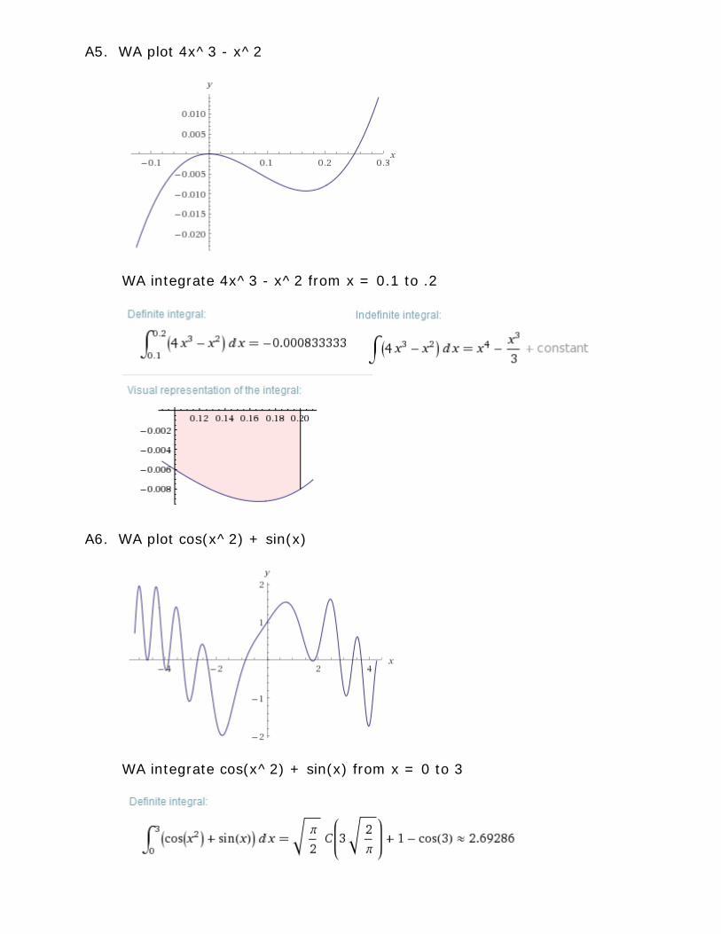
A5. WA plot 4x^3 - x^2

WA integrate 4x^3 - x^2 from x = 0.1 to .2

A6. WA plot cos(x^2) + sin(x)

WA integrate cos(x^2) + sin(x) from x = 0 to 3

A7. WA plot sin(x^2) - cos(x)

WA integrate sin(x^2) - cos(x) from x = -2 to 2

A8. WA plot 4e^(x^3)

WA integrate 4e^(x^3) from x = 0.5 to 1.0

A9. WA plot ln(5x^2 + sin(x))

WA integrate ln(5x^2 + sin(x)) from x = -4 to -2

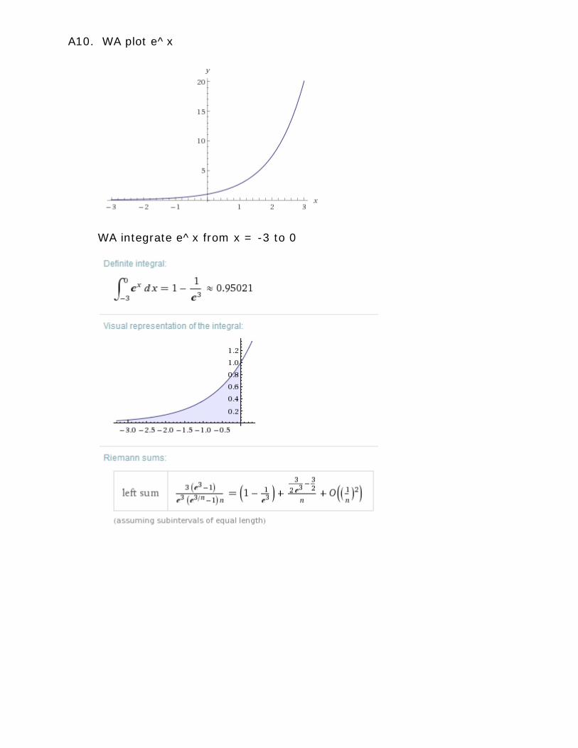
A10. WA plot e^x

WA integrate e^x from x = -3 to 0

1

T5 C16 Applications of Integration Areas

Represent the area as a group of one or more functions. Then apply integration to find the enclosed areas

One function

Let y = f(x). Then the area under the graph of f from a to b is just the integral of f(x) from a to b.

Note: This will be the NET AREA, A, so if some of the area is positive, A1, and some is negative, A2, then A= A1–A2

Example 1. Find the area under the graph of

g(t)=t2

Integrate t^2 + .2sin(15t) from t = .5 to 2.5 A=5.15822

+ .2sin(15t) from t = .5 to 2.5

Note: I could have used x as the independent variable.

Note: WA also gives the graph and the anti-derivative.

In the old days we would have found the anti-derivative with techniques of integration and evaluated it at .5 and 2.5 to find the definite integral.

The anti-derivative is t3

A = (2.5)

/3 – (1/75)cos(15t) 3/3–cos(15X2.5)/75–(.5)3

= 5.208 - .0109 - .0417 + .0046 = 5.16

/3+ cos(15X.5)/75

Even with a calculator this would take several minutes, longer for me since I make a lot of careless mistakes and must check my work several times before I am confident of the answer.

Pre-calculator days it would take a lot longer with a slide rule or log tables and trig tables.

2

Example 2. g(t)= [t2 + .2sin(15t)]1/2

WA Integrate (t^2 + .2sin(15t))^.5 from t = .5 to 2.5

from t = .5 to 2.5

Answer: 2.99841

There is no easy anti-derivative. This problem would not be included in a calculus book. It has to be “solved” by an approximation technique that only a computer can perform efficiently and quickly.

Example 3. f(x) = sin(x) from 1.5 to 4.5

WA Integrate sin(x) from x=1.5 to 4.5

Answer: .281533

Note: the graph. Some of the area is positive and some negative. The answer is the NET area.

Example 4. f(x) = lsin(x)l from x = 1.5 to 4.5

WA Integrate absolute value (sin(x)) from x=1.5 to 4.5

Answer: 1.85994

Notice the graph. All areas are positive now.

3

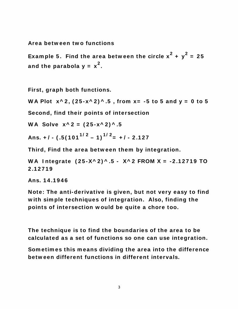
Area between two functions

Example 5. Find the area between the circle x2 + y2 = 25

and the parabola y = x2

.

First, graph both functions.

WA Plot x^2, (25-x^2)^.5 , from x= -5 to 5 and y = 0 to 5

Second, find their points of intersection

WA Solve x^2 = (25-x^2)^.5

Ans. +/- (.5(1011/2 – 1)1/2

Third, Find the area between them by integration.

= +/- 2.127

WA Integrate (25-X^2)^.5 - X^2 FROM X = -2.12719 TO 2.12719

Ans. 14.1946

Note: The anti-derivative is given, but not very easy to find with simple techniques of integration. Also, finding the points of intersection would be quite a chore too.

The technique is to find the boundaries of the area to be calculated as a set of functions so one can use integration.

Sometimes this means dividing the area into the difference between different functions in different intervals.

4

Example 6 Multiple intervals

Find the area whose upper boundary is the parabola

y – 10 = -(x – 1)

and whose lower boundary is the two circles

2

(x + 2)2 + y2 = 25 and (x - 2)2 + y2

WA Plot 10-(x-1)^2,(25 -(x+2)^2)^.5,(25 -(x-2)^2)^.5, from x=-5 to 5

= 25

Now we need to find the correct intervals by determining the points of intersection of these three curves.

WA Solve 10-(x-1)^2 = (25 -(x+2)^2)^.5

Answer: -1.24872

WA Solve 10-(x-1)^2 = (25 -(x-2)^2)^.5

Answer we care about: 3.27259

WA Solve (25 -(x+2)^2)^.5=(25 -(x-2)^2)^.5

Answer: 0

So now we can find the area with two integrals over two intervals.

WA Integrate 10-(x-1)^2 -(25 -(x+2)^2)^.5 from -1.24872 to 0 Answer: 3.04582

WA Integrate 10-(x-1)^2 -(25 -(x-2)^2)^.5 from 0 to 3.27259 Answer 12.4601

Total Area 3.04582 + 12.4601 = 15.50592

Try this without WA to feel sympathy for our ancestors.

5

Example 7. What is the difference between the catenary cosh(x) and a parabola?

The parabola through the points (0,b) and (a,0) and (-a,0) is y = (a – b)x2

cosh(0) = 1, and cosh(1) = cosh(-1) = 1.543

+ b

So, y = .543x2

WA7-1 Plot cosh(x), .543x^2 +1 from x = -1 to 1

+ 1 is the parabola passing through the catenary at (-1, cosh(-1)),(0,cosh(0)), and (1,cosh(1))

We can see why Galileo thought it was a parabola

WA7-2 Integrate cosh(x)- .543x^2 -1 from x = -1 to 1

Wow. Only .0116 difference in area. Which was higher?

Clearly the parabola.

T5 C16 Applications of Integrations – Areas Exercises

Q1. Find the graph and definite integral for the function f(x) = cos(x) from -2π to 2π.

Q2. Find the graph and the absolute value of the definite integral for the function f(x) = cos(x) from -2π to 2π.

Q3. Find the graph and definite integral for the function f(x) = sin(x)+sin2

Q4. Find the graph and the absolute value of the definite integral for the function f(x) = sin(x)+sin

(x) from 0 to 2π.

2

Q5. Plot the graph for the functions f(x) = -x

(x) from 0 to 2π.

2 and f(x) = x2

x = -1 to 1, then find their points of intersection and the area between the two functions.

-1 from

Q6. Plot the graph for the functions f(x) = x2

Q7. Plot the graph for the functions f(x) = -x

and f(x) = sin(x), then find their points of intersection and the area between the two functions.

2

Q8. Plot the graph for the functions f(x) = 3x

+ 5 and f(x) = cos(x), then find their points of intersection and the area between the two functions.

2

Q9. Plot the graph for the functions f(x) = -x

- 7 and f(x) = sin(x), then find their points of intersection and the area between the two functions.

2 +8, (x + 4)2 + y2

(x-4) = 16,

2 + y2

Q10. Plot the graph for the functions f(x) = sin(x), f(x) = cos(x), x=0, from

= 16, then find their points of intersection and the area between the three functions.

x= 0 to π, then find their points of intersection and the area between the three functions.

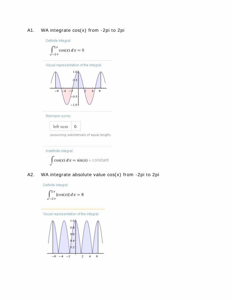
A1. WA integrate cos(x) from -2pi to 2pi

A2. WA integrate absolute value cos(x) from -2pi to 2pi

A3. WA integrate sin(x) + sin^2(x) from 0 to 2pi

A4. WA integrate absolute value sin(x) + sin^2(x) from 0 to 2pi

A5. WA plot -x^2, x^2-1 from x = -1 to 1

WA solve -x^2 = x^2-1

Points of intersection: x = ±1/20.5

WA integrate -x^2 - (x^2-1) from x = -0.707107 to 0.707107

= ±0.707107

Area: 0.942809

A6. WA plot x^2, sin(x)

WA solve sin(x) = x^2

Points of intersection: x = 0, 0.876726

WA integrate sin(x) - (x^2) from x = 0 to 0.876726

Area: 0.135698

A7. WA plot –x^2 + 5, cos(x)

WA solve –x^2 + 5 = cos(x)

Points of intersection: x = ±2.39451

WA integrate -x^2 + 5 - cos(x) from x = -2.39451 to 2.39451

Area: 13.4332

A8. WA plot 3x^2 - 7, sin(x)

WA solve 3x^2 - 7 = sin(x)

Points of intersection: x = -1.41563, 1.63280

WA integrate sin(x) - (3x^2 - 7) from x = -1.41563 to 1.63280

Area: 14.3655

A9. WA plot -x^2 +8, (16 -(x+4)^2)^.5, (16 -(x-4)^2)^.5 from x = -4 to 4

Points of intersection: WA solve -x^2+8 = (16 -(x+4)^2)^.5

x = -2.11474

WA solve -x^2+8 = (16 -(x-4)^2)^.5

x = 2.11474

WA solve (16 -(x+4)^2)^.5 = (16 -(x-4)^2)^.5

x = 0

Area: WA integrate (-x^2+8)-((16 -(x+4)^2)^.5) from x = -2.11474 to 0

area = 8.4508

WA integrate (-x^2+8) - ((16 -(x-4)^2)^.5) from x = 0 to 2.11474

area = 8.4508

Total area = 16.9016

A10. WA plot sin(x), cos(x), x=0, from x= 0 to pi

Points of intersection: WA solve sin(x) = cos(x)

x = 0.785398

WA solve sin(x) = 0

x = 3.14159

WA solve cos(x) = 0

x = 1.57080

Area: WA integrate sin(x) – cos(x) from x = 0.785398 to 1.57080

area = 0.414217

WA integrate sin(x) - 0 from x = 1.57080 to 3.14159

area = 0.999996

Total area = 1.414213

T5 C17 Applications of Integration Arc Length

Suppose you would like to know the length of the graph of f(x) from (a,f(a)) to (b,f(b)).

The answer is the integral of [1 + (f’(x))2]1/2

Here’s why.

from a to b.

Divide the interval (a,b) into subintervals a0 to an

The distance from (a

. Each subinterval has length h=(b – a)/n

i,f(ai)) to (ai+1,f(ai+1

[(f(a

) would be

i+1) - f(ai))2 + (ai+1 - ai)2]

= [(f(a

1/2

i + h) - f(ai))2 + h2]

= [{(f(a

1/2

i + h) - f(ai))/h}2 + 1]1/2

Now the Arc Length is approximated by

X h

SUM [{(f(ai + h) - f(ai))/h}2 + 1]1/2

If h = dx is an infinitesimal, then this becomes

X h i = 1,…n

Infinite Sum [{(f(x+dx) - f(x))/dx}2 + 1]1/2

Integral [(f’(x))

X dx OR

2 + 1]1/2

This heuristic argument can be made as rigorous as you wish when you treat the Hyperreal number system rigorously.

as x = a to b

Example 1. Find the arc length of a semicircle of radius 1. Of course, we know the answer is ∏.

f(x) = (1 – x2)1/2

f’(x) = -x(1 – x

has a graph which is this semi circle/

2)-1/2

So, [1 + (f’(x)

2]1/2 = [1/(1 - x2)]

Thus, arc length is Integral [1/(1 - x

1/2

2)]1/2

WA Integrate (1/(1 - x^2))^.5 from -1 to 1

from x= -1 to 1

But, WA can do this directly.

WA Arc Length (1 – x^2)^.5 from x = -1 to 1

Note: the Integral this was interpreted as.

Example 2. What is the length of the parabola f(x) = x

From (1,1) to (3,9)?

2

WA Arc length x^2 from x=1 to 3 Ans: 8.268

Note the Integral

Example 3. What is the length of one cycle of the sine curve?

WA Arc length sin(x) from x = 0 to 2Pi Ans: 7.6404

Note: It didn’t matter whether f(x) was above or below the axis, unlike areas.

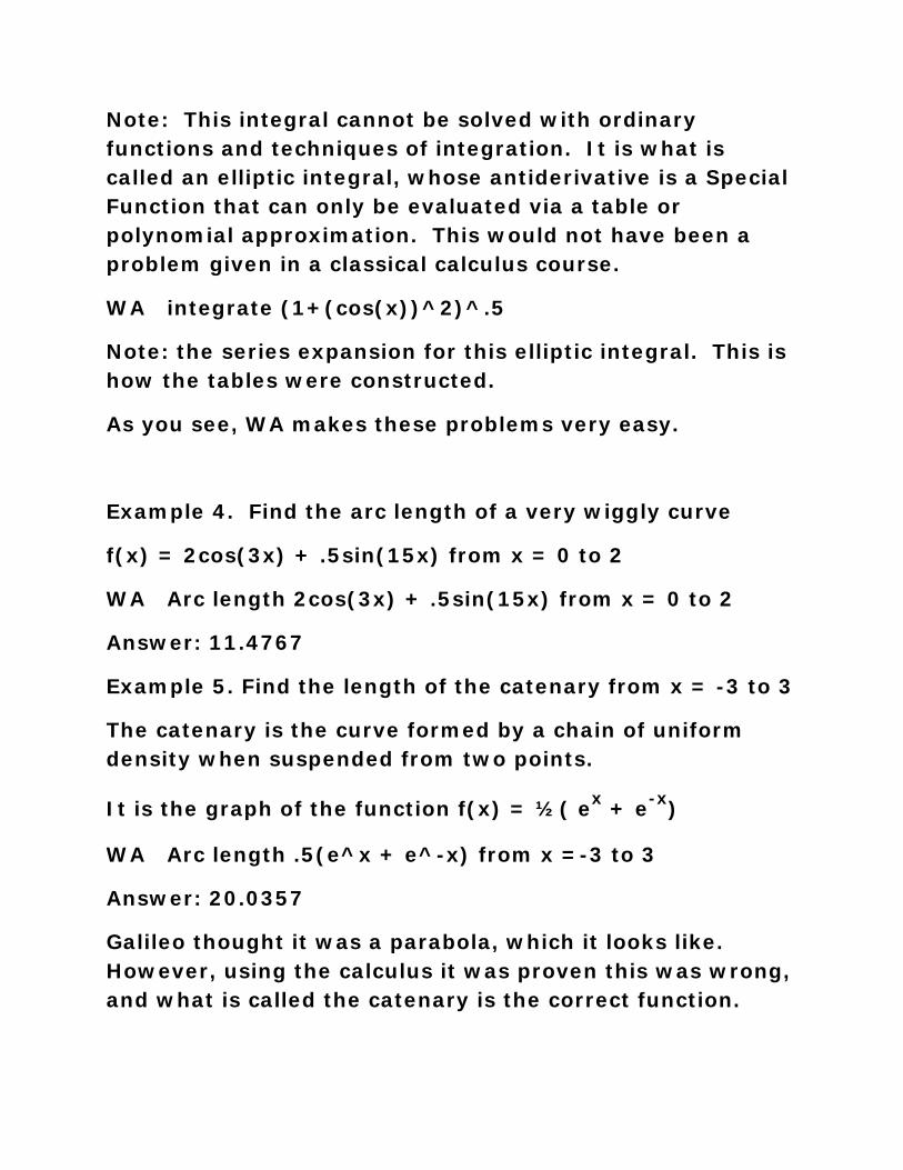
Note: This integral cannot be solved with ordinary functions and techniques of integration. It is what is called an elliptic integral, whose antiderivative is a Special Function that can only be evaluated via a table or polynomial approximation. This would not have been a problem given in a classical calculus course.

WA integrate (1+(cos(x))^2)^.5

Note: the series expansion for this elliptic integral. This is how the tables were constructed.

As you see, WA makes these problems very easy.

Example 4. Find the arc length of a very wiggly curve

f(x) = 2cos(3x) + .5sin(15x) from x = 0 to 2

WA Arc length 2cos(3x) + .5sin(15x) from x = 0 to 2

Answer: 11.4767

Example 5. Find the length of the catenary from x = -3 to 3

The catenary is the curve formed by a chain of uniform density when suspended from two points.

It is the graph of the function f(x) = ½( ex + e-x

WA Arc length .5(e^x + e^-x) from x =-3 to 3

)

Answer: 20.0357

Galileo thought it was a parabola, which it looks like. However, using the calculus it was proven this was wrong, and what is called the catenary is the correct function.

As you can see, it is very difficult to solve many of these problems with the classical tools of calculus.

WA makes it very easy.

This is why a tool like WA is mandatory for any STEM professional.

You can use WA to explore many examples.

Just make them up and play with it.

You may go to engineering and science books and look for examples to play with.

Just imagine what our ancestors would have done with WA and thought of it. Sort of like much of our modern technology like smart phones, GPS, airplanes, computers, TV, etc.

Unfortunately, most current calculus textbooks and courses are as antiquated as a horse and buggy. Yes, the horse and buggy were great technologies in their day, and very difficult to master. But, what value is it to master these obsolete technologies today?

You must learn a WA type of tool today if you are going to compete in the STEM marketplace.

And, your mastery of calculus (and later differential equations and linear algebra and more) will be much easier and more thorough.

Practice and play with WA until it is as easy for you as a video game or smart phone.

T5 C17 Applications of Integrations – Arc Length Exercises

Find the arc length for the following functions.

Q1. f(x) = cos(x) from x = 0 to 2π.

Q2. f(x) = sin(x)+sin2

Q3. f(x) = 4x

(x) from x = 0 to 2π.

3 + 6x2

Q4. f(x) = e

- 8x from x = -2 to 2.

x

Q5. f(x) = e

from x = 1 to 3.

x – e-x

Q6. f(x) = (x-1)/(x

from x = -1.5 to 0.

2

Q7. f(x) = sin(2x)+sin(1.1x) from x = 0 to 3π.

+ x) from x = 1 to 5.

Q8. f(x) = cos(3x) + cos(x) from x = 0 to 2π.

Q9. (x) = cos(3x) - cos(2x) from x = 0 to 2π.

Q10. f(x) = tan(x) from x = 0 to π/2.

A1. WA arc length cos(x) from x = 0 to 2pi

A2. WA arc length sin(x)+sin^2(x) from x = 0 to 2pi

A3. WA arc length 4x^3 + 6x^2 - 8x from x = -2 to 2

A4. WA arc length e^x from x = 1 to 3

A5. WA arc length e^x – e^(-x) from x = -1.5 to 0

A6. WA arc length (x-1)/(x^2 + x) from x = 1 to 5

A7. WA arc length sin(2x)+sin(1.1x) from x = 0 to 3pi

A8. WA arc length cos(3x) + cos(x) from x = 0 to 2pi

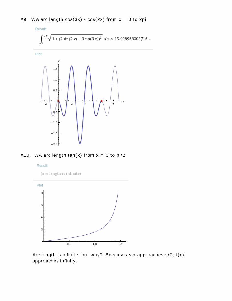
A9. WA arc length cos(3x) - cos(2x) from x = 0 to 2pi

A10. WA arc length tan(x) from x = 0 to pi/2

Arc length is infinite, but why? Because as x approaches π/2, f(x) approaches infinity.

T5 C18 Applications of Integration Volume Disc Method

Let f(x) be a function defined with derivative over (a,b)

Rotate f(x) about the x-axis to form a volume of revolution

What is this volume?

Slice the volume into very thin discs with thickness, dx.

The area of the disc at x will be Pi[f(x)]

The volume of the disc at x will be AreaXdx = Pi[f(x)]

2

2

So the volume of the of the revolution will be

dx

Integral Pi[f(x)]2

dx from a to b.

Example 1. Rotate the parabola f(x) = y = x2

WA1 integrate pix^4 from 0 to 2 Ans.20.106

about the xaxis from 0 to 2. What is its volume.

Or, we can do it directly with WA as follows:

WA2 volume of revolution x^2 from 0 to 2

Example 2. What is the volume of a sphere? Rotate the circle f(x) = (1 – x2)1/2

WA3 integrate pi(1 – x^2) from -1 to 1 Ans. 4Pi/3 of course

about the x axis?

WA4 volume of revolution (1-x^2)^.5 from x = -1 to 1

Of course, you can integrate from any limits. For example, suppose you just want the volume of the right hemisphere.

WA5 integrate pi(1 – x^2) from 0 to 1

WA6 volume of revolution (1-x^2)^.5 from x = 0 to 1

Example 3. Rotate a sine about the xaxis

WA7 volume of revolution sin(x) from x = 0 to Pi

Ans: Pi2

Example 4. Rotate a cosine about the x axis for one cycle

/2

WA8 volume of revolution of cos(x) from 0 to 2Pi

Note: WA also gave us the surface area. But, we will discuss that in another Lesson, C20

Example 4. Volume of Revolution of

f(x) = x2

WA9

+ 1 + .5sin(15x) from x = .5 to 1.9

Volume of revolution x^2+1+.5sin(15x) from x=.5 to 1.9

Ans. 35.597 Note the integral

Also, note the surface area of the Solid

Historically, it was easy to set up the integral. The difficulty was in evaluating it.

Now, WA makes this very easy too.

Indeed, WA will let you evaluate problems that were essentially intractable historically if one could not find an anti-derivative with ordinary functions.

Example: Find the volume of the solid of revolution of sin(x2

WA10 volume of revolution of sin(x^2) from 0 to 2Pi

) from 0 to 2Pi

It is easy to set up the integral, but difficult to integrate it since it involves a special function. The ordinary techniques of integration would not solve it easily.

WA11 integrate (sin(x^2)^2

The antiderivative is a Special Function.

We can also find the volume of a solid of revolution of an area enclosed between two functions

y = f(x) and y = g(x) from a to b where f(x) > g(x)

Integral Pi[f2(x) – g2

Example: what is the volume of the solid of revolution enclosed between the parabolas y = x

(x)] from a to b.

1/2 and y = x2

WA12 Plot x^.5,x^2 from 0 to 1

?

WA13 Integrate Pi(x – x^4) from 0 to 1

Ans: .94248

Now we could calculate the volume of the solid of revolution for the larger function and then subtract the volume of the solid of revolution for the smaller function.

WA14 volume of solid of revolution x^.5 from 0 to 1

Ans. 1.5780

WA15 volume of solid of revolution x^2 from 0 to 1

Ans. .628319

Note 1.5780 - .628319 = .94248

Now there is another way using what is called the shell method we will learn about in the next lesson C19

WA16 integrate 2Pix(x^.5 – x^2) from 0 to 1

If you can find a way to do this directly with a volume of revolution command please post it to the Forum or email it to me.

T5 C18 Applications of Integration – Volume – Disc Method Exercises:

Find the volume for the following functions, rotated about the x-axis.

Q1. f(x) = sin(x)+sin2

Q2. f(x) = e

(x) from x = 0 to 2π. x

Q3. f(x) = (x-1)/(x

from x = 1 to 3.

2

Q4. f(x) = sin(2x)+sin(x) from x = 0 to 2π.

+ x) from x = 1 to 5.

Q5. f(x) = ex – e-x

Q6. f(x) = e

from x = -3 to 3.

x + 5x2

Q7. f(x) = 5x + sin(3x) from x = -2π to 2π.

from x = -2 to 2.

Q8. f(x) = cos(2x) from x = 0 to 2π.

Q9. f(x) = -x2 and f(x) = x2-1 from x = - 0.707107 to 0.707107. f(x) = –x2 is the smaller function, and f(x) = x2

Q10. f(x) = -x

-1 is the larger function.

2

f(x) = -x + 5 and f(x) = cos(x) from x = -2.39451 to 2.39451.

2

+ 5 is the larger function, and f(x) = cos(x) is the smaller function.

A1. WA volume of revolution sin(x)+sin^2(x) from x = 0 to 2pi

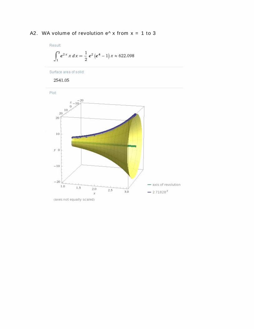
A2. WA volume of revolution e^x from x = 1 to 3

A3. WA volume of revolution (x-1)/(x^2 + x) from x = 1 to 5

A4. WA volume of revolution sin(2x) + sin(x) from x = - to 2pi

A5. WA volume of revolution e^x - e^-x from x = -3 to 3

A6. WA volume of revolution e^x + 5x^2 from x = -2 to 2

A7. WA volume of revolution 5x + sin(3x) from x = -2pi to 2pi

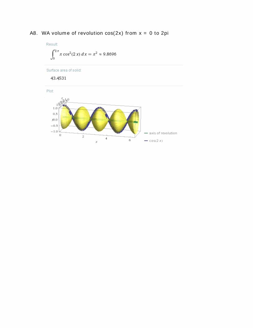
A8. WA volume of revolution cos(2x) from x = 0 to 2pi

A9. larger: WA volume of revolution x^2 – 1 from x = -0.707107 to 0.707107

smaller: WA volume of revolution -x^2 from x = -0.707107 to 0.707107

Volume: 3.18407 – 0.222144 = 2.961926

A10. larger: WA volume of revolution -x^2 + 5 from x = -2.39451 to 2.39451

smaller: WA volume of revolution cos(x) from x = -2.39451 to 2.39451

volume: 187.504 – 5.95639 = 181.54761

 

T5 C19 Applications of Integral Volume Shell Method

We can rotate the region enclosed between the parabolas f(x) = x1/2 and g(x) = x3 from 0 to 1 about the x-axis using the disc method

by integrating Pi[(f(x))2 – (g(x))2]dx from 0 to 1.

WA1 integrate Pi(x – x^6) from 0 to 1

WA2 volume of solid of revolution of region between x^.5 and x^3 from 0 to 1 about the x axis

Now suppose we want to rotate this same region about the y axis?

We can use what is called the shell method whereby we integrate 2Pix[f(x) – g(x)]dx from 0 to 1

Do you see why?

[f(x) – g(x)]dx is the area of a thin vertical strip which is x units from the y axis. We rotate this strip about the y axis to get a shell of volume 2Pix[f(x) – g(x)]dx since 2Pix is the circumference of a circle of radius x.

WA3 integrate 2Pix(x^.5 – x^3) from 0 to 1

WA4 volume of solid of revolution of region between x^.5 and x^3 from 0 to 1 about the y axis

We can use either the disc method or the shell method, whichever is easier to set up and integrate.

Or, we can simply use WA, and we also then get the picture of the solid of revolution.

 

Let’s now look at the region of the intersection of two circles.

Example

WA5 Plot (x-7)^2 + (y-8)^2 - 25=0, (x-3)^2 + (y-8)^2 - 36=0 from -5 to 15

Suppose we want to rotate around the x axis. Which would be easier to use, disc or shell?

Answer. Probably neither since we have to divide the region into two subregions.

Around the y axis? Disc or shell.

Same answer.

But, what if we exchanged the x and y, or reflected in the 45o line y = x? We would get the same shape region. Only now rotating about the x axis would be like rotating the original region about the y axis, and vica versa.

WA6 Plot (y-7)^2 + (x-8)^2 - 25=0, (y-3)^2 + (x-8)^2 - 36=0 from 0 to 15

Now we have two functions.

The upper function would be:

WA7 Solve for y, (y-3)^2 + (x-8)^2 - 36=0

The lower function would be:

WA8 Solve for y, (y-7)^2 + (x-8)^2 - 25=0

 

We also need to know the two points of intersection so we know the limits on the x axis

WA9 Solve (y-7)^2 + (x-8)^2 - 25=0, (y-3)^2 + (x-8)^2 - 36=0

Now, we can calculate the volume of the solid of revolution about the x axis

WA 10 Volume of solid of revolution of region between 3+(-x^2+16x-28)^.5 and 7-(-x^2+16x-39)^.5 from 3.039 to 13 around the x axis

Now the volume of revolution about the y axis

WA 11 Volume of solid of revolution of region between 3+(-x^2+16x-28)^.5 and 7-(-x^2+16x-39)^.5 from 3.039 to 13 around the y axis

Unable to compute, although gave a picture. So we use shell method

WA12 Integrate 2Pix(3+(-x^2+16x-28)^.5 – (7-(-x^2+16x-39)^.5)) from 3.039 to 12.96

Answer: 2580.41

Observe how complicated the antiderivative is in this last example.

An alternative way to do this last one, would be to go back to the original region and divide it into two parts and rotate about the x axis. Do you see why this would give you the same answer.

 

WA5 Plot (x-7)^2 + (y-8)^2 - 25=0, (x-3)^2 + (y-8)^2 - 36=0 from -5 to 15

We need to know the points of intersection, in particular the x coordinate.

WA13 solve (x-7)^2 + (y-8)^2 - 25=0, (x-3)^2 + (y-8)^2 - 36=0

Answer: 6.375

Divide the little circle into two functions.

WA14 solve for y, (x-7)^2 + (y-8)^2 - 25=0

Find the volume of the solid of revolution of this first subregion

WA15 volume of solid of revolution of region between 8 +(-x^2+14x-24)^.5 and 8 -(-x^2+14x-24)^.5 from 0 to 6.375 around the x axis

Answer: 1660.58

Now the second region.

WA16 solve for y, (x-3)^2 + (y-8)^2 - 36=0

WA17 volume of solid of revolution of region between 8 +(-x^2+6x+27)^.5 and 8 -(-x^2+6x+27)^.5 from 6.375 to 12 around the x axis

Answer: 919.83

Total Volume 1660.58 + 919.83 = 2580.41

See WA12

 

So we see we can use either the disc method or shell method, whichever is easier.

In the old days, finding the antiderivative so we could apply the FTC and find the definite integral was also a very important consideration.

Now, WA eliminates this consideration.

Furthermore, WA will often just give you the answer directly and you don’t even have to set up the disc or shell integrals.

However, you still need to graph the functions or the region and consider the proper limits and functions.

But, as you have seen WA even makes this easy compared to the old manual methods.

And, we used fairly simple quadratic examples here. WA works with virtually any functions, even those that would have been totally impractical to deal with classically.

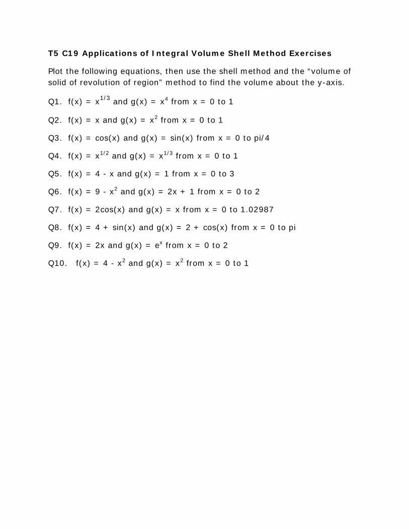
T5 C19 Applications of Integral Volume Shell Method Exercises

Plot the following equations, then use the shell method and the “volume of solid of revolution of region” method to find the volume about the y-axis.

Q1. f(x) = x1/3 and g(x) = x4 from x = 0 to 1

Q2. f(x) = x and g(x) = x2 from x = 0 to 1

Q3. f(x) = cos(x) and g(x) = sin(x) from x = 0 to pi/4

Q4. f(x) = x1/2 and g(x) = x1/3 from x = 0 to 1

Q5. f(x) = 4 - x and g(x) = 1 from x = 0 to 3

Q6. f(x) = 9 - x2 and g(x) = 2x + 1 from x = 0 to 2

Q7. f(x) = 2cos(x) and g(x) = x from x = 0 to 1.02987

Q8. f(x) = 4 + sin(x) and g(x) = 2 + cos(x) from x = 0 to pi

Q9. f(x) = 2x and g(x) = ex from x = 0 to 2

Q10. f(x) = 4 - x2 and g(x) = x2 from x = 0 to 1

A1. WA plot x^1/3 and x^4 from x = 0 to 1

WA integrate 2pix((x^1/3)-(x^4)) from x = 0 to 1

WA volume of region between x^1/3 and x^4 from 0 to 1 about the y axis

A2. WA plot x and x^2 from x = 0 to 1

WA integrate 2pix((x)-(x^2)) from x = 0 to 1

WA volume of solid of revolution of region between x and x^2 from 0 to 1 about the y axis

A3. WA plot cos(x) and sin(x) from x = 0 to pi/4

WA integrate 2pix((cos(x))-(sin(x))) from x = 0 to pi/4

WA volume of solid of revolution of region between cos(x) and sin(x) from 0 to pi/4 about the y axis

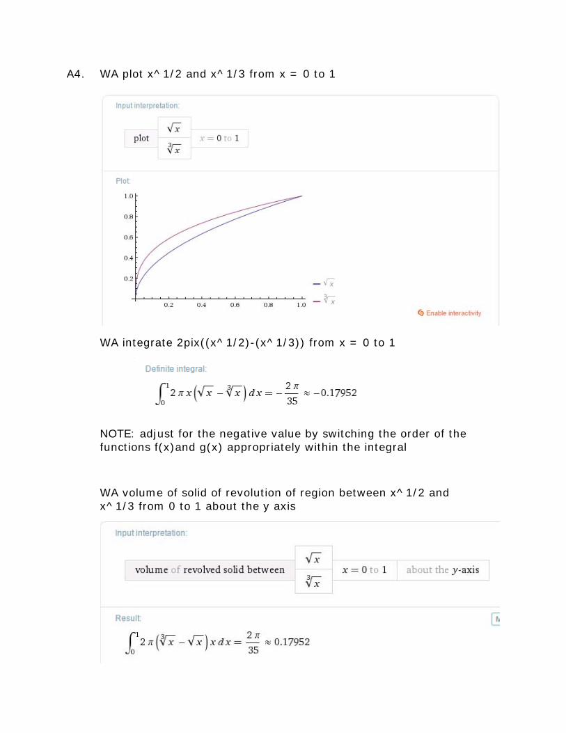
A4. WA plot x^1/2 and x^1/3 from x = 0 to 1

WA integrate 2pix((x^1/2)-(x^1/3)) from x = 0 to 1

NOTE: adjust for the negative value by switching the order of the functions f(x)and g(x) appropriately within the integral

WA volume of solid of revolution of region between x^1/2 and x^1/3 from 0 to 1 about the y axis

A5. WA plot 4 - x and 1 from x = 0 to 3

WA integrate 2pix((4 - x)-(1)) from x = 0 to 3

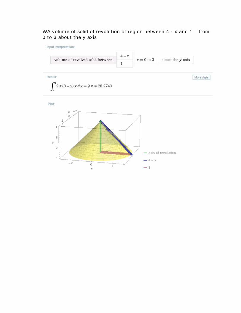
WA volume of solid of revolution of region between 4 - x and 1 from 0 to 3 about the y axis

A6. WA plot 9 - x^2 and 2x + 1 from x = 0 to 2

WA integrate 2pix((9 - x^2)-(2x + 1)) from x = 0 to 2

WA volume of solid of revolution of region between 9 - x^2 and 2x + 1 from 0 to 2 about the y axis

A7. WA plot 2cos(x) and x from x = 0 to 1.02987

WA integrate 2pix((2cos(x))-(x)) from x = 0 to 1.02987

WA volume of solid of revolution of region between 2cos(x) and x from 0 to 1.02987 about the y axis

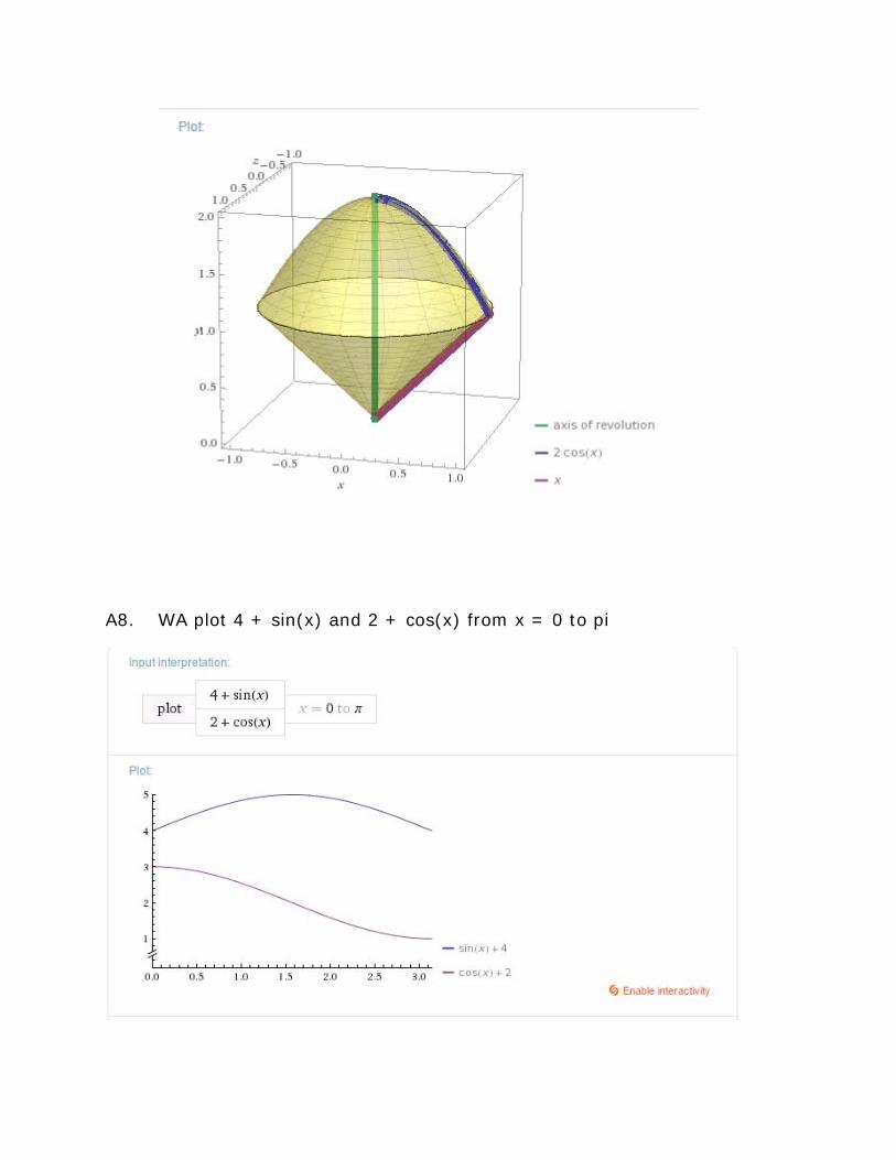
A8. WA plot 4 + sin(x) and 2 + cos(x) from x = 0 to pi

WA integrate 2pix((4 + sin(x))-(2 + cos(x))) from x = 0 to pi

WA volume of solid of revolution of region between 4 + sin(x) and 2 + cos(x) from 0 to pi about the y axis

A9. WA plot 2x and e^x from x = 0 to 2

WA integrate 2pix((2x)-(e^x)) from x = 0 to 2

NOTE: flip the negative

WA volume of solid of revolution of region between 2x and e^x from 0 to 2 about the y axis

A10. WA plot 4 - x^2 and x^2 from x = 0 to 1

WA integrate 2pix((4 - x^2)-(x^2)) from x = 0 to 1

WA volume of solid of revolution of region between 4 - x^2 and x^2 from 0 to 1 about the y axis

T5 C20 Applications of Integration Surface of Revolution

Let f(x) be a differentiable function from a to b.

Rotate the graph of f(x) about the x axis.

What is the surface area of this solid of revolution?

Area = Integral 2Pif(x)[1 + (f’(x))2]1/2

Why? See Diagram which you should draw.

dx from a to b

Note: We slice the surface into little slices. Then we compute the area of the slice.

2Pif(x) is the radius of slice from the x axis, and

[1 + (f’(x))2]1/2

So, 2Pif(x)[1 + (f’(x))

dx is the length of the little piece of the slice. See the Diagram

2]1/2

The Integral adds them all up.

dx is the area of this little slice.

Do you see the similarity with the arc length formula?

It is good to start with a surface of revolution we already know the answer to, a sphere whose surface area is 4Pi.

Example 1. The surface are of the sphere of radius 1?

f(x) = (1 – x2)1/2 and f’(x) = -x(1 – x2)

and [1 + (f’(x))

-1/2

2]1/2 = [1 – (-x(1 – x2)-1/2 )2]1/2

[1 + x

=

2(1 – x2)-1]1/2 = [1 – x2]-1/2

So, 2Pif(x)[1 + (f’(x))

2]1/2

= 1Pi(1 – x

dx =

2)1/2[1 – x2]-1/2

So, the surface area of the sphere is just

= 2Pidx

Integral of 2Pidx from -1 to 1

Now, this was a lot of work setting up the integral, and then easy to do the integration.

WA1 Integrate 2Pi, from x = -1 to 1

Could WA have made this easier?

Of course!

WA2 surface of revolution (1-x^2)^.5 from x= -1 to 1

And, we get the picture of the surface of the sphere

Example 2. The surface area of a paraboloid which is the surface of revolution of f(x) = x2

WA3 surface of revolution x^2 from x= 1 to 4

from 1 to 4.

Notice the graph, and also it told us the volume too.

Well, I’ll admit this takes out the fun and frustrates all the classical calculus courses. So let’s play the game.

Integral 2Pif(x)[1 + (f’(x))2]1/2

f’(x) = 2x, so

dx from 1 to 4

Integral 2Pix2[1 + 4x2]1/2

WA4 Integrate 2Pix^2(1 + 4x^2)^.5 from x = 1 to 4

from 1 to 4

Well, we got the same answer: 812.76

Notice, how much fun must it have been to find this anti-derivative. Just look at it! In the old classical days, this would have been a very challenging problem. Easy to set up the integral, but difficult to find the antiderivative. Also, Notice there is no nice 3D graph.

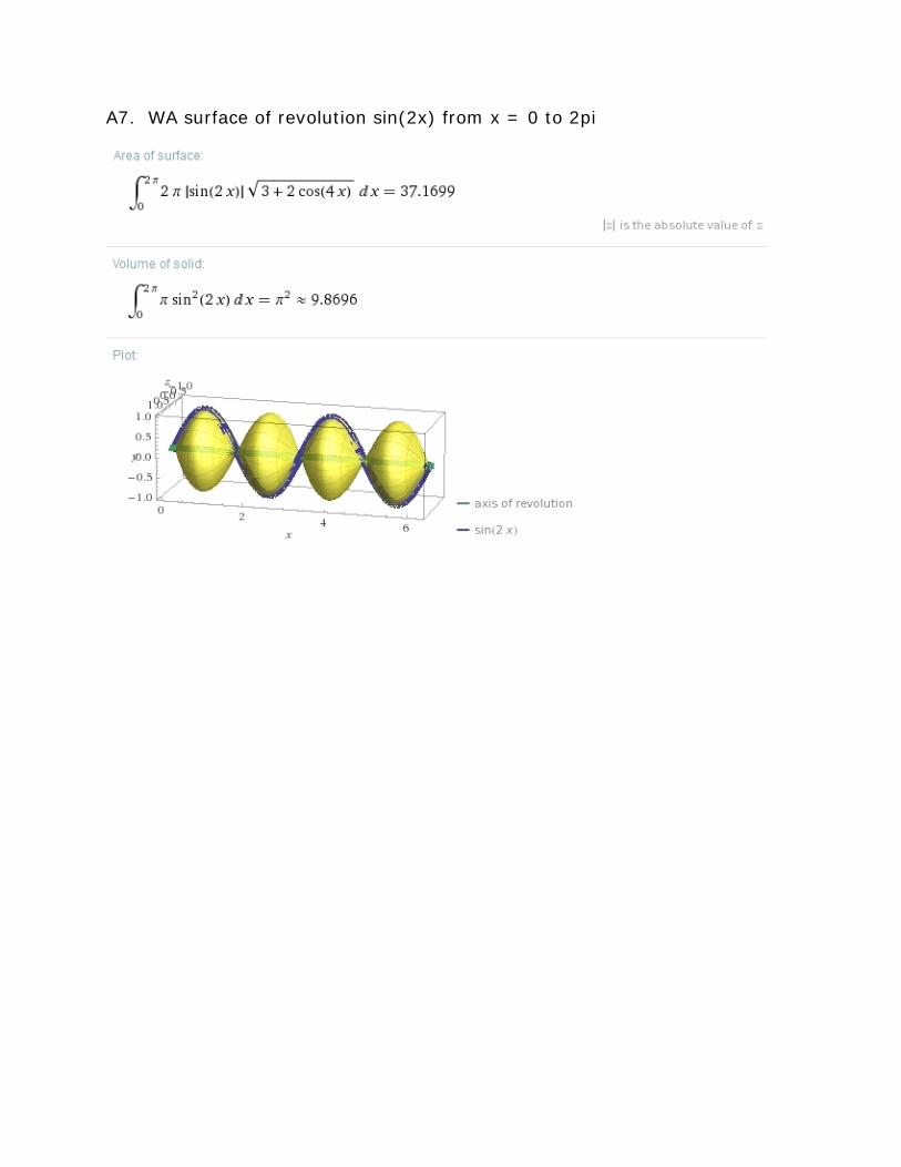
Example 3 Surface area of the solid of revolution of sin(x) from x = 0 to Pi. WA5 surface of revolution sin(x) from x= 0 to Pi Ans: 14.426 Also, Volume is 4.9348 If you are a glutton for punishment, then do it the classical way. f’(x) = cos(x) Integral 2Pisin(x)[1 + (cos(x))2]1/2

from 0 to Pi

WA6 integrate 2PiSin(x)(1+(cos(x))^2)^.5 from x = 0 to Pi Easy to set up the integral, But, wouldn’t it be fun to find that anti-derivative! Our classical ancestors must have had so much fun! Do you see why students who have to learn calculus the classical way have so much difficulty? Frankly, until tools like WA came along, calculus was a tool that was often very difficult to use, or in many cases impossible when one couldn’t find an anti-derivative. It often forced scientist and engineers to build mathematical models that were simplistic approximations just so they could solve the calculus, or Diff Eq, problems.

T5 C20 Applications of Integration– Surface of Revolution Exercises

Find the surface for the following functions, rotated about the x-axis.

Q1. f(x) = sin(x)+sin2(x) from x = 0 to 2π.

Q2. f(x) = ex from x = 1 to 3.

Q3. f(x) = (x-1)/(x2 + x) from x = 1 to 5.

Q4. f(x) = sin(2x)+sin(x) from x = 0 to 2π.

Q5. f(x) = ex – e-x from x = -3 to 3.

Q6. f(x) = 3x3 from x = -2 to 2 .

Q7. f(x) = sin(2x) from x =0 to 2π.

Q8. f(x) = cos(3x) - sin(2x) from x =0 to π.

Q9. f(x) = ex + x from x =0 to 2.

Q10. f(x) = 2x - ex^2 from x = -1 to 1.

A1. WA surface of revolution sin(x) + sin^2(x) from x = 0 to 2pi

A2. WA surface of revolution e^x from x= 1 to 3

A3. WA surface of revolution (x - 1)/(x^2 + x) from x = 1 to 5

A4. WA surface of revolution sin(2x) + sin(x) from x = 0 to 2pi

A5. WA surface of revolution e^x - e^-x from x = -3 to 3

A6. WA surface of revolution 3x^3 from x = -2 to 2

A7. WA surface of revolution sin(2x) from x = 0 to 2pi

A8. WA surface of revolution cos(3x) - sin(2x) from x = 0 to pi

A9. WA surface of revolution e^x + x from x = 0 to 2

A10. WA surface of revolution 2x - e^(x^2) from x = -1 to 1

T5 C21 Parametric Functions

By definition the graph of y = f(x) can have only one point on any vertical line. That is, f(x) is a unique number for any x.

This creates a problem when we want to analyze a graph which folds back on itself, which is often the case.

For example, the graph of y2

WA 1 Plot y^2=x from x = 0 to 2

= x, which is a parabola.

Of course, in this case it can be represented as two different functions. y = x1/2 and y = -x

WA 2 Plot x^.5,-x^.5 from x=0 to 2

1/2

But, there is another way to handle this,

Parametric Functions.

Let t be the independent variable ranging from a to b.

Graph (f(t),g(t)) from (f(a),g(a)) to (f(b),g(b)) in the x-y plane. t is called a parameter.

In this example, let f(t)=t2

Why? (x,y) ≡ (y

and g(t)=t and -2<t<2

2,y) ≡ (t2

WA 3 Parametric Plot (t^2,t)

, t) when t = y

WA 4 Parametric Plot (t^2,t) from t = -2 to 2

Note: WA also gave us the arc length. We will discuss this in a later lesson in detail.

Ok, now let’s look at another familiar example, the circle of radius R centered at the origin.

The graph of x2 + y2 = R2 can be split into two functions representing the upper semicircle and lower semicircle as you well know. y = (R2 – x2)1/2 and y = -(R2 – x2)

You also know that if the parameter t, representing angles in radian measure is utilized, then any point (x, y) on the circle t radians from the positive x axis can also be represented by trig functions. (x,y) = (Rcos(t), Rsin(t))

1/2

So we can now deal with the circle with a parametric representation. Let’s say R = 7

WA 5 Parametric Plot (7cos(t),7sin(t))

Ok, let’s check the arc length. 2Pi7 = 14Pi

WA 6 Parametric Plot (7cos(t),7sin(t)) from t =0 to 2Pi

You might want to pause and try some other circles, and even ellipses yourself now.

OK, now what extra abilities do parametric representations give us?

The answer is that we can now deal with much more complex graphs. This was not of too much use classically, since it was so laborious to plot a parametric graph.

But, with a tool like WA it is now very easy.

WA 7 Parametric Plot (t^4 - 3t^2, t)

Note: if y = t, then x = y4 – 3y2

Imagine how difficult this would be to split up into ordinary functions. You would have to solve a 4

is what we plotted.

th

With Parametric Functions we can get some really interesting graphs that would be essentially impossible with just regular y = f(x) functions.

degree polynomial in y to get functions in terms of x.

WA 8 Parametric Plot (t + 2sin(2t),t + 2cos(5t))

But, we can control the parameter limits

WA 9 Parametric Plot (t + 2sin(2t),t + 2cos(5t)) from t = -5Pi to 5Pi

Imagine trying to handle this with regular functions.

Note. The Arc Length is also calculated here too. In the next lesson we will look at how this is done.

Now, the facts are that you can take a whole course involving parametric representations of curves, and higher dimensional surfaces.

This is used extensively in modern Computer Aided Design (CAD) systems.

Obviously, it has applications in the arts.

And, it can be used in animation systems to create very entertaining animations.

So, play with the WA and try lots of things for yourself.

Then, as you proceed with your career you may learn much more about the applications of this wonderful “technology”.

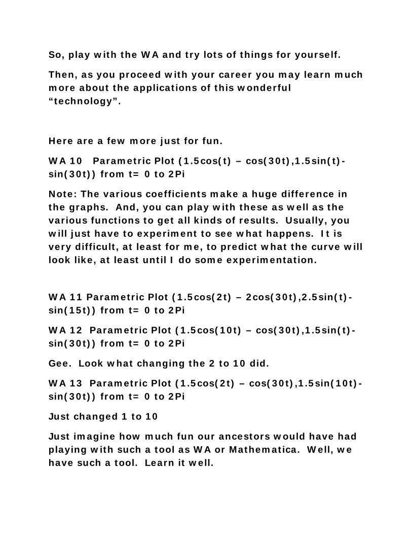
Here are a few more just for fun.

WA 10 Parametric Plot (1.5cos(t) – cos(30t),1.5sin(t)-sin(30t)) from t= 0 to 2Pi

Note: The various coefficients make a huge difference in the graphs. And, you can play with these as well as the various functions to get all kinds of results. Usually, you will just have to experiment to see what happens. It is very difficult, at least for me, to predict what the curve will look like, at least until I do some experimentation.

WA 11 Parametric Plot (1.5cos(2t) – 2cos(30t),2.5sin(t)-sin(15t)) from t= 0 to 2Pi

WA 12 Parametric Plot (1.5cos(10t) – cos(30t),1.5sin(t)-sin(30t)) from t= 0 to 2Pi

Gee. Look what changing the 2 to 10 did.

WA 13 Parametric Plot (1.5cos(2t) – cos(30t),1.5sin(10t)-sin(30t)) from t= 0 to 2Pi

Just changed 1 to 10

Just imagine how much fun our ancestors would have had playing with such a tool as WA or Mathematica. Well, we have such a tool. Learn it well.

Add in animation and color and 3D capabilities, which Mathematica does, and you have a really amazing new world.

This is the world we live in today. This is the world you must learn your mathematics in. Just imagine how this will impact your STEM studies. One last example. . .

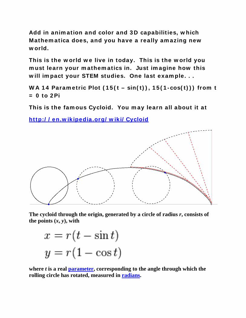
WA 14 Parametric Plot (15(t – sin(t)), 15(1-cos(t))) from t = 0 to 2Pi

This is the famous Cycloid. You may learn all about it at

http://en.wikipedia.org/wiki/Cycloid

The cycloid through the origin, generated by a circle of radius r, consists of the points (x, y), with

where t is a real parameter, corresponding to the angle through which the rolling circle has rotated, measured in radians.

T5 C21 Parametric Functions Exercises

Q1. Given the function x = y4

Q2. Given the function x = y

, plot the parametric function using t as an independent variable, from -2<t<2.

4 + 3y3 – 10y2

Q3. Given the function x = e

, plot the parametric function using t as an independent variable, from -6<t<6.

y^2 - e3y

Q4. Given the function for a circle x

, plot the parametric function using t as an independent variable, from -10<t<10.

2 + y2 = r2

Q5. Given the function for a circle x

where r=5, plot the parametric function using t as an independent variable, from t = 0 to 2π.

2 + y2

Q6. Given the function for an ellipse x

= 9, plot the parametric function using t as an independent variable, from t = 0 to 2π.

2/9 + y2

Q7. Given the function for an ellipse x

/4 = 1, plot the parametric function using t as an independent variable, from t = 0 to 2π.

2 + y2

Q8. Plot the following functions as a parametric function: f(t) = t - sin(3t), g(t) = t + 3cos(4t) from -3<t<3.

/16 = 1, plot the parametric function using t as an independent variable, from t = 0 to 2π.

Q9. Plot the following functions as a parametric function: f(t) = t2

Q10. Plot the following functions as a parametric function: f(t) = 2t

- sin(t), g(t) = t + 3sin(3t) from -5<t<5.

2

- 3sin(t), g(t) = t + 3sin(3t) from -5<t<5.

A1. WA parametric plot (t^4, t) from -2<t<2

A2. WA parametric plot (t^4 + 3t^3 - 10t^2, t) from -6<t<6

A3. WA parametric plot (e^(t^2) - e^(3t),t) from -10<t<10

A4. WA parametric plot (5cos(t),5sin(t)) from t =0 to 2Pi

A5. WA parametric plot (3cos(t),3sin(t)) from t = 0 to 2pi

A6. x2/9 + y2/4 = 1, or x2/32 + y2/22

WA parametric plot (3cos(t),2sin(t)) from t =0 to 2Pi

= 1

A7. x2 + y2/16 = 1, or x2/12 + y2/42

WA parametric plot (cos(t),4sin(t)) from t =0 to 2Pi

= 1

Note the different scales WA used for the x-axis and y-axis. That’s why it looks like a circle.

A8. WA parametric plot (t - sin(3t), t + 3cos(4t)) from -3<t<3

A9. WA parametric plot (t^2 - sin(t), t + 3sin(3t)) from -5<t<5

A10. WA parametric plot (2t^2 - 3sin(t), t + 3sin(3t)) from -5<t<5