table of contents 3. hydrodynamics 8 · table of contents page 1. executive summary 2 2....

TABLE OF CONTENTS

Page

1. EXECUTIVE SUMMARY 2

2. INTRODUCTION 6

3. HYDRODYNAMICS 8

3.1 Regional Setting .......................................................................................................................... 8 3.1.1 Tides 8 3.1.2 Circulation 14 3.1.3 Residence Time 16 3.1.4 Wind-waves 17 3.1.5 Salinity 18

3.2 Project Setting ........................................................................................................................... 20 3.2.1 Tributary Inflows 20 3.2.2 Salinity 22

4. SEDIMENT DYNAMICS 26

4.1 Regional Setting ........................................................................................................................ 26 4.1.1 Geological Evolution 26 4.1.2 Bathymetry 27 4.1.3 Sediment Transport 28 4.1.4 Sediment Budget 30 4.1.5 Spring Phytoplankton Bloom 30

4.2 Project Setting ........................................................................................................................... 31 4.2.1 Tributary Sediment Load 31 4.2.2 Sediment Characteristics 32 4.2.3 Pond Bottom Elevations and Subsidence 32 4.2.4 Marsh Sedimentation 33

5. REFERENCES 36

6. LIST OF PREPARERS 42

TABLES Table 1 – Harmonic constants for San Francisco Bay 11 Table 2 – Harmonic constants for San Mateo Bridge, west side 12 Table 3 – Harmonic constants for Dumbarton Bridge 13 Table 4 – Approximate range in salinities expected for each type of pond management 24 Table 5 – Measured sedimentation data and MARSH98 SSC indices 34

South Bay Salt Pond Restoration Project March 2005

Hydrodynamics and Sediment Dynamics Existing Conditions i 1750.01

FIGURES Figure 1 – South San Francisco Bay vicinity map Figure 2 – Tidal height variations within South Bay Figure 3 – Tidal variability in San Francisco Bay Figure 4 – Typical annual tidal variability Figure 5 – USGS monitoring site locations Figure 6 – Delta outflow Figure 7 – Bay Bridge near-surface and near-bottom salinity Figure 8 – San Mateo Bridge near-surface and near-bottom salinity Figure 9 – Dumbarton Bridge near-surface salinity Figure 10 – Channel Marker 17 near-surface and near-bottom salinity Figure 11 – Delta outflow and South Bay near-surface salinity Figure 12 – Longitudinal salinity profiles from a dry winter (1991) and a wet winter (1998) Figure 13 – Longitudinal salinity profiles over time during an El Nino year (1998) Figure 14 – Moffat and Nichol instrument location Figure 15 – Daily streamflow measurements for Coyote Creek @ Highway 237 Figure 16 – Daily streamflow measurements for Guadalupe River @ Highway 101 Figure 17 – Daily streamflow measurements for Alameda Creek near Niles Figure 18 – Daily streamflow measurements for Alameda Creek Flood Control Channel @ Union City Figure 19 – Daily streamflow measurements for San Francisquito Creek @ Stanford University Figure 20 – Daily streamflow measurements for Matadero Creek @ Palo Alto Figure 21 – Initial Stewardship Plan, Eden Landing Complex Figure 22 – Initial Stewardship Plan, Ravenswood Complex Figure 23 – Initial Stewardship Plan, Alviso Complex Figure 24 – 1983 South Bay bathymetry Figure 25 – Bay Bridge mid-depth and near bottom SSC Figure 26 – San Mateo Bridge mid-depth and near-bottom SSC Figure 27 – Dumbarton Bridge mid-depth and near-bottom SSC Figure 28 – Channel Marker 17 mid-depth and near-bottom SSC Figure 29 – Channel Marker 17 mid-depth and near-bottom SSC, short-term variability Figure 30 – Longitudinal suspended particulate matter profiles during an El Nino winter (1998) Figure 31 – Longitudinal phytoplankton biomass profiles during an El Nino winter (1998) Figure 32 – Longitudinal suspended particulate matter profiles during summer (1998) Figure 33 – Longitudinal phytoplankton biomass profiles during summer (1998) Figure 34 – Long-term variability in spring bloom magnitude Figure 35 – Suspended sediment concentrations in Alameda Creek near Niles Figure 36 – Suspended sediment concentrations in Guadalupe River @ Highway 101 Figure 37 – Suspended sediment concentrations in Guadalupe River @ San Jose Figure 38 – Pond Bathymetry, Eden Landing Complex Figure 39 – Pond Bathymetry, Alviso Complex Figure 40 – Sedimentation monitoring locations Figure 41 – Measured sedimentation data and Marsh 98 sedimentation curves


Hydrodynamics and Sediment Dynamics Existing Conditions ii 1750.01

ABBREVIATIONS AND ACRONYMS ACFCC Alameda Creek Flood Control Channel Bay San Francisco Bay cfs cubic feet per second CO-OPS Center for Operational Oceanographic Products and Services Central Bay Central San Francisco Bay chl a Chlorophyll a Corps U.S. Army Corps of Engineers Delta San Francisco Bay Delta far South Bay portion of the South Bay south of the Dumbarton Bridge ISP Initial Stewardship Plan km kilometer l liter LiDAR Light Detection and Ranging m meter mg milligrams mgd million gallons per day mm millimeter MHHW mean higher high water MHW mean high water MLLW mean lower low water MLW mean low water NCDC National Climate Data Center NGVD29 National Geodetic Vertical Datum of 1929 NOAA National Oceanic and Atmospheric Administration NOS National Ocean Service NSW Nearshore Spectral Wave Model OBS Optical backscatter ppt parts per thousand PORTS Physical Oceanographic Real-Time System RMP Regional Monitoring Program S second SBSP South Bay Salt Pond SCVWD Santa Clara Valley Water District SPM Suspended particulate matter SSC Suspended sediment concentration SWAN Simulating WAves Nearshore South Bay South San Francisco Bay TRIM Tidal Residual Intertidal Mudflat USGS U.S. Geological Survey USFWS U.S. Fish and Wildlife Service yr year


Hydrodynamics and Sediment Dynamics Existing Conditions iii 1750.01


Hydrodynamics and Sediment Dynamics Existing Conditions 1 1750.01

1. EXECUTIVE SUMMARY

This document presents the existing conditions for hydrodynamics and sediment dynamics within the South Bay Salt Pond (SBSP) Restoration Project area and South San Francisco Bay (South Bay), providing baseline data for restoration planning and environmental compliance. This document is one of a series of existing conditions reports, with companion documents for biology and habitats, flood management and infrastructure, water and sediment quality, and public access and recreation. This report draws on the scientific literature, recent San Francisco Bay and South San Francisco Bay (South Bay) reports, data collected by local and government agencies, and previous SBSP Restoration Project reports. Extensive data collection by the United States Geological Survey and others, along with numerous modeling studies, has increased the general understanding of South Bay hydrodynamics. South Bay sediment dynamics are not as well understood. Presented below is a summary of the existing hydrodynamic and sediment dynamic conditions documented in this report. Hydrodynamics. South Bay can be characterized as a large shallow basin, with a relatively deep main channel surrounded by broad shoals and mudflats. Tidal currents, wind, and freshwater tributary inflows interact with this complex bathymetry to define the residual circulation patterns, residence time, and determine the level of vertical mixing and stratification. The enclosed nature of the South Bay creates a mix of progressive and standing wave behavior, which leads to tidal amplification southward. The tidal range at the Golden Gate Bridge is approximately 5.6 feet, and southward at the Dumbarton Bridge it increases to approximately 8.5 feet. The tides in San Francisco Bay are mixed semidiurnal, with two high and two low tides of unequal heights each day. The tides exhibit strong spring-neap variability, with the spring tides (larger tidal range) occurring during the full and new moon, and neap tides (smaller tidal range) occurring during the moon’s quarters. The tides also vary on an annual cycle, with the strongest spring tides occurring in May/June and November/December, and the weakest neap tides occurring in March/April and September/October, The most important factor influencing circulation patterns in South Bay is bathymetry. Bathymetric variations create differences in the flow patterns north of the San Bruno shoal, between the San Bruno shoal and the San Mateo Bridge, between the San Mateo Bridge and Dumbarton Bridge, and south of the Dumbarton Bridge. Circulation patterns also differ between the deep main channel and the expansive shoals. In the channel, the tidal excursion varies between 6.2 and 12.4 miles; and in the subtidal shoals which typically experience weaker tidal currents, it varies between 1.9 and 4.8 miles, with much smaller excursions occurring on the intertidal mudflats. In general, there is a northward tidally-driven residual current along the eastern shoal, with a counter-clockwise gyre directly north of the San Mateo Bridge, and a clockwise gyre directly south of the San Bruno shoal. Below the San Mateo Bridge, residual flows are generally weak. The presence of wind alters the tidally-driven circulation patterns, most notably in broad areas conducive to developing a long fetch. Wind-driven circulation typically results in a wind-driven surface layer in the



direction of the wind, coupled with a return flow in the deeper layers. In the South Bay the most significant winds are the onshore breezes blowing inland from the ocean to the Central Valley during the daytime on hot days during the spring and summer. These northwesterly winds create a clockwise wind-driven circulation pattern, with a southerly flow along the eastern shoals, and a northward flow in the main channel. In the winter, southwesterly winds drive a counter-clockwise wind-driven circulation pattern, with currents towards the northeast on the eastern shoals. Although there is wide annual variation, the South Bay generally has a wet winter/spring season, and a dry summer season. Therefore, the majority of the freshwater tributary inflows enter the South Bay during the winter and spring; during the dryer summer months, the major source of freshwater is effluent from municipal wastewater treatment plants. The largest South Bay tributaries are Alameda Creek (which flows into the Alameda Creek Flood Control Channel), Guadalupe River (which flows into Alviso Slough), and Coyote Creek (which becomes a tidal slough and connects directly with the South Bay). Salinity. Salinity in the South Bay is governed by the salinity in Central San Francisco Bay (Central Bay), exchange between South and Central Bays, freshwater inflows to South Bay, and evaporation. Generally, the South Bay is vertically well mixed (i.e. there is little tidally-averaged vertical salinity variation) with near oceanic salinities (33 parts per thousand), although areas within the far South Bay (below the Dumbarton Bridge) remain brackish year-round due to wastewater treatment plant discharges. Seasonal variations in salinity are driven primarily by seasonal variability in freshwater inflow, both locally and from the San Francisco Bay Delta (Delta). While extended periods of below average rainfall are common in the San Francisco area, years of much higher than normal precipitation, and therefore large freshwater inflows, are also common due to El Niño conditions in the Pacific. During wet winters when Delta outflow exceeds 200,000 cubic feet per second, freshwater from the Delta can intrude into the South Bay and push surface salinities below 10 parts per thousand. This phenomenon can cause vertical density stratification (freshwater overlaying denser saline water) in the main South Bay channel. High inflows from the local tributaries in the far South Bay can also set up density stratification in the main channel, as well as stratification on tidal time scales in the tributaries and sloughs themselves. Water circulation and salinities within the three SBSP Restoration Project pond complexes are currently being managed in order to avoid concentrating salt within the ponds and to lower salinities to meet salinity discharge requirements. Cargill currently retains the management of certain ponds within the Ravenswood and Alviso complexes due to high pond salinities. Full transition of these ponds to the U.S. Fish and Wildlife Service is expected to occur by 2012. Sediment Dynamics. Bay habitats – subtidal shoals, intertidal mudflats, and wetlands – are directly influenced by sediment availability, transport and fate, specifically the long-term patterns of deposition and erosion. Understanding the processes which have led to the formation and evolution of the South Bay is a key factor for predicting future evolution. The South Bay has been shaped by processes acting at the geologic timescale (thousands of years), as well as processes at shorter timescales, such as tides (hours), the spring-neap tidal cycle (days), freshwater inflows (weeks), seasonal winds (months), and ecological



and climactic change (years). The South Bay has also been shaped by anthropogenic causes, such as the conversion of 90 percent of the tidal salt marsh areas to salt ponds, agriculture, and urban development. Characterization of existing sediment dynamics includes bathymetry, sediment transport, and the overall sediment budget. The primary mechanisms affecting the bathymetry are erosion, sedimentation, and the exchange of suspended sediments with the Central Bay. The bathymetry of the South Bay has undergone significant change over the past century, due to both anthropogenic and natural causes, and the South Bay has shifted between a depositional and erosional environment. During the most recent sediment budget period analyzed, between 1956 and 1983, the South Bay was erosional causing a net export of sediment to the Central Bay. Although the South Bay as a whole has undergone periods of net deposition and net erosion, the far South Bay below Dumbarton Bridge has remained largely depositional since bathymetric data collection began in 1857. The transport and fate of suspended sediment has the potential to affect the transport and fate of contaminants, such as metals and pesticides, and the distribution of nutrients which are essential for primary productivity at the base of the food web. Increasing suspended sediment concentrations (SSC) are also directly correlated with increasing turbidity and decreasing light availability, thus affecting photosynthesis, primary productivity, and phytoplankton bloom dynamics. SSCs in the South Bay exhibit highly dynamic short-term variability, primarily in response to spring-neap variations in tidally driven resuspension, wind driven resuspension, and riverine input from local tributaries and sloughs. SSCs also exhibit longer-term seasonal variability. In the winter and early spring, the main sources of suspended sediments are local tributaries and the Central Bay. There is typically little direct input of suspended sediment in the dryer summer months; however, SSCs are typically higher due to increased wind-wave resuspension and re-working of previously deposited sediments. Extremely wet (El Niño) years can deliver turbid plumes of sediment from the Delta into the South Bay. This influx of sediment enters the system and is continually reworked and transported as it is deposited and resuspended by tidal- and wind-driven currents. Several successive dry winters (e.g. drought conditions) can result in significant reductions in SSCs throughout the year due to reductions in the supply of sediment for internal redistribution. The main losses of sediment from the South Bay are export to the Central Bay, and sediment capture within marsh areas and restored ponds. Sediments are carried into a marsh or restored pond and deposited on flood tides, causing the marsh or mudflat area to increase in elevation. Sediments are also carried out on ebb tides when wind-waves cause erosion or inhibit cohesive sediment deposition. The rate of sedimentation depends on SSCs near the marsh or restored pond location, the elevation of the ground surface within the tidal frame, and the degree to which tidal exchange to the site is restricted. Sedimentation data from several recently restored sites within the South Bay is analyzed and reviewed, with the highest sedimentation rates found near the Alviso Complex.



2. INTRODUCTION

This document provides the existing conditions for hydrodynamics and sediment dynamics for the South Bay Salt Pond (SBSP) Restoration Project. A map of the project vicinity is provided in Figure 1. The goal of the project is to restore and enhance a mix of wetlands, while integrating restoration with flood management, and also providing public access and recreation opportunities. In order to accomplish the restoration goal, it is necessary to have an understanding the existing natural landscape. This report is one volume in a set of five existing conditions reports. Additional volumes include: • Biology and Habitats • Water and Sediment Quality • Flood Management and Infrastructure • Public Access and Recreation Additional companion documents include the Data Summary Report (PWA and others 2004a), the Initial Opportunities and Constraints Summary Report (PWA and others 2004b), and the Mercury Technical Memorandum (Brown and Caldwell 2004). South San Francisco Bay (South Bay) is a geographically and hydrodynamically complex system, with freshwater tributary inflows, tidal currents, and wind stress on the water surface interacting with complex bathymetry to drive circulation patterns (Walters 1982). The bathymetry of the South Bay, characterized by a deep, narrow channel surrounded by broad shoals and mudflats, is the most important factor influencing circulation patterns (Cheng and Smith 1985). Understanding the residual circulation and residence times in the South Bay is important to SBSP restoration efforts because these processes influence the potential movement patterns of suspended sediment and other water quality constituents. Suspended sediment concentrations (SSC) in South Bay exhibit highly dynamic, short-term variability, primarily in response to riverine input from tributaries and sloughs, spring-neap variations in tidally driven resuspension, and wind driven resuspension (Cloern and others 1989; Powell and others 1989; Schoellhamer 1996). Wind is probably the most dynamic factor affecting temporal and spatial variability of SSC, resulting in a redistribution of sediments within the estuary (May and others 2003). The major external sediment inputs to the South Bay are tributary sediment load and exchange between Central San Francisco Bay and South Bay (Krone 1992). Restoring ponds to tidal inundation will alter the existing bathymetry of the South Bay through changes in geomorphic processes, increases in tidal prism, and modified connections with tributary sloughs. The resulting bathymetric change will in turn alter tidal currents and circulation patterns. In order to understand the magnitude of the changes under consideration, it is necessary to first characterize the baseline existing hydrodynamic and sediment dynamic conditions.



The Hydrodynamics and Sediment Dynamics Existing Conditions Report contains the following sections: • Section 3. Hydrodynamics. This section presents the existing conditions for hydrodynamics in the

South Bay, including tides, circulation, waves, freshwater inflows, and salinity. • Section 4. Sediment Dynamics. This section presents the existing conditions for sediment

dynamics in the South Bay, including bathymetry, sediment transport, and the sediment budget.



3. HYDRODYNAMICS

3.1 Regional Setting South San Francisco Bay (South Bay) is a large shallow basin, with a relatively deep relict river channel surrounded by broad shoals and mudflats. The width of the Bay ranges from less than 1.2 miles (2 km) near the Dumbarton Bridge (the Dumbarton Narrows) to more than 12 miles (20 km) north of the San Mateo Bridge. The mean depth of the Bay is less than 13 feet (4 m), with a channel depth of 33 – 50 feet (10 – 15 m). The intertidal areas contain a network of small branching channels that effectively drain these areas at low water, leaving an expanse of exposed mudflats. South Bay is both a geographically and hydrodynamically complex system, with freshwater tributary inflows, tidal currents, and wind stress on the water surface interacting with complex bathymetry. These forcing mechanisms define the residual circulation patterns and residence time, and determine the level of vertical mixing and stratification. 3.1.1 Tides

Tidal flows contribute to erosion and sedimentation that affect the formation and shape of the channels and inlets in the South Bay (Life Science 2004). Extensive data collection by the U.S. Geological Survey (USGS) and others (e.g., Cheng and Gartner 1984), and numerous modeling studies (e.g., Cheng and others 1993; Gross and others 1999; URS 2002) has contributed to the general understanding of the overall hydrodynamics. Tidal Regime Tides propagate through the narrow opening at the Golden Gate (see Figure 5) as shallow water waves, and the amplitudes and phases of the waves are modified by the bathymetry, reflections from the shores, the Earth’s rotation, and bottom friction. The enclosed nature of the South Bay creates a mix of progressive wave and standing wave behavior, where the wave is reflected back upon itself (Walters and others 1985). The harmonic addition of the original wave plus the reflected wave leads to tidal amplitude increases, or tidal amplification. This amplification causes the tidal range to increase southward, from about 5.6 feet (1.7 m) at the Golden Gate, to 8.5 feet (2.6 m) at the Dumbarton Bridge (Schemel 1995). The tidal energy propagates down the main South Bay channel and is dispersed into the broad shoal areas (Walters and others 1985). In the South Bay, the nature of the standing wave causes slack water to occur at high and low tide, and the maximum currents occur between high and low water. Tidal currents are stronger in the channel than in the shoals (Walters and others 1985), therefore slack water generally occurs in the shoals before the channel (Life Science 2004). For a pure standing wave, the tide will rise and fall at the same time everywhere in the basin. As shown on Figure 2, the tides do rise and fall at nearly the same time at several South Bay stations; however, because the observed tide does not consist of a single wave, but rather the superposition of many tide waves of difference frequency and amplitude, the tide does not exhibit pure



standing wave behavior. There is approximately a 40 minute phase difference from Hunters Point to the Dumbarton Bridge due to a substantial degree of progressive wave behavior (Figure 2). Tidal Variability The tides in San Francisco Bay are mixed semidiurnal, with two high and two low tides of unequal heights each day (see Figure 3). In addition, the tides exhibit strong spring-neap variability, with the spring tides (larger tidal range) occurring approximately every two weeks during the full and new moon. Spring tides exhibit the greatest difference between successive high and low tides. Neap tides (smaller tidal range) occur approximately every two weeks during the moon’s quarters, and exhibit the smallest difference between successive highs and low tides. Figure 3 depicts a typical spring-neap tidal cycle. The tides also vary on an annual cycle, with the strongest spring tides occurring in May/June and November/December, and the weakest neap tides occurring in March/April and September/October (Figure 4). The National Oceanic and Atmospheric Administration (NOAA) and the National Ocean Service (NOS) predict water surface elevation data in the South Bay at Oyster Point Marina, Hunters Point, San Mateo Bridge, Dumbarton Bridge, and Redwood City. The only real-time operational tide gauge in the South Bay is located in Redwood Creek, near the Port of Redwood City. This gauge is part of the Physical Oceanographic Real-Time System (PORTS) installed in 1998 by NOAA in San Francisco Bay. PORTS allows access to real time data (24 hours in the past, and 24 hour projections to the future) of Bay-wide wind distribution, tides, tidal currents, and salinity (Cheng and Gartner 1985). Tidal current data was collected by the USGS and NOAA at several stations throughout the Bay during the 1980s, with the largest concentration of current meters located in the deep main channel (Gartner and Walters 1986). Harmonic Constants A tide is essentially the movement of water caused by astronomical phenomena, such as the way the earth, moon and sun move in relation to each other and the force of gravity. These movements, or interactions, occur in regular cycles or frequencies, for example:

• 12 hour repeated cycle due to the gravity of the sun • 12.42 hour repeated cycle due to the gravity of the moon • 24 hour repeated cycle due to interactions with the sum • 24.83 hours repeated cycle due to interactions with the moon

Each of these cycles is called a harmonic constituent, and its frequency (or period) is known accurately. Associated with each harmonic constituent is the tidal amplitude (equal to one half of the range), and the time of arrive (phase), which are referred to as harmonic constants and are unique for a given location. The harmonic constants allow its individual contribution to the overall tide to be determined forward or backward in time almost indefinitely. Adding up the effects of all the individual harmonic constituents at a given location allows the overall tide to be predicted at any time in the future or past. Defining the harmonic constants for the South Bay is therefore an important component for hindcasting and forecasting hydrodynamic conditions.



NOAA, NOS, and the Center for Operational Oceanographic Products and Services (CO-OPS) maintain a database of harmonic constants that can be used for tide predictions. Tables 1-3 depicts the harmonic constants for San Francisco Bay, from the tide station located at the Presidio, near the Golden Gate Bridge, as well as the harmonic constants for South Bay at the west side of San Mateo Bridge and the Dumbarton Bridge. The primary constituents for the South Bay are the principal diurnal (K1) and the principal semidiurnal (M2) as noted by their large amplitudes. The letters refer to the principal astronomical driver of the cycle, such as M and L for lunar, S for solar, and K for lunar-solar interactions. The subscripts of the constituents refer to the number of cycles per day, with 1 referring to one cycle per day (diurnal), 2 to two cycles per day (semidiurnal), and so forth. The tidal amplification in the South Bay is also evident from the harmonic constants, as the M2 constituent increases from 1.903 ft at the Presidio, to 2.710 at the San Mateo Bridge, and 3.038 ft at the Dumbarton Bridge.



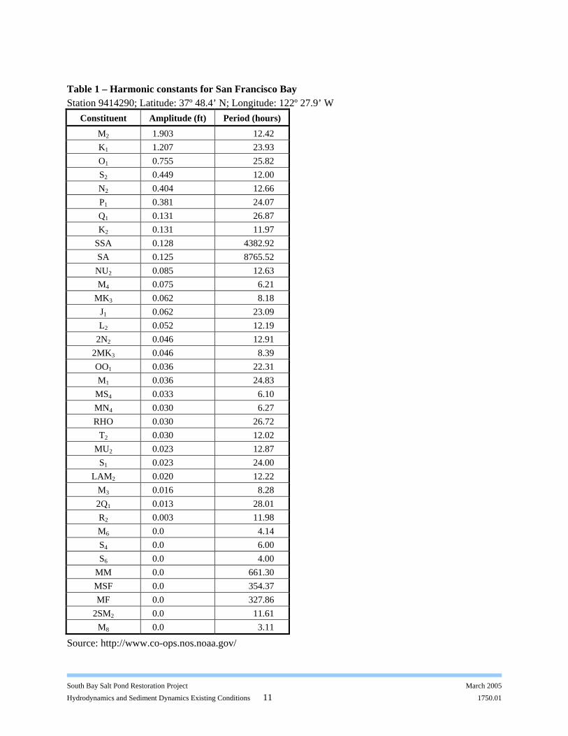
Table 1 – Harmonic constants for San Francisco Bay Station 9414290; Latitude: 37º 48.4’ N; Longitude: 122º 27.9’ W

Constituent Amplitude (ft) Period (hours)

M2 1.903 12.42 K1 1.207 23.93 O1 0.755 25.82 S2 0.449 12.00 N2 0.404 12.66 P1 0.381 24.07 Q1 0.131 26.87 K2 0.131 11.97

SSA 0.128 4382.92 SA 0.125 8765.52 NU2 0.085 12.63 M4 0.075 6.21

MK3 0.062 8.18 J1 0.062 23.09 L2 0.052 12.19

2N2 0.046 12.91 2MK3 0.046 8.39 OO1 0.036 22.31 M1 0.036 24.83

MS4 0.033 6.10 MN4 0.030 6.27 RHO 0.030 26.72

T2 0.030 12.02 MU2 0.023 12.87

S1 0.023 24.00 LAM2 0.020 12.22

M3 0.016 8.28 2Q1 0.013 28.01 R2 0.003 11.98 M6 0.0 4.14 S4 0.0 6.00 S6 0.0 4.00

MM 0.0 661.30 MSF 0.0 354.37 MF 0.0 327.86

2SM2 0.0 11.61 M8 0.0 3.11

Source: http://www.co-ops.nos.noaa.gov/



Table 2 – Harmonic constants for San Mateo Bridge, west side Station 9414458; Latitude: 37º 34.8’ N; Longitude: 122º 15.2’ W


M2 2.710 12.42 K1 1.316 23.93 O1 0.791 25.82 S2 0.597 12.00 N2 0.545 12.66 P1 0.413 24.07 K2 0.203 11.97 Q1 0.141 26.87

NU2 0.128 12.63 SSA 0.128 4382.92 SA 0.125 8765.52 L2 0.125 12.19

2MK3 0.115 8.39 MK3 0.069 8.18

J1 0.066 23.09 MU2 0.056 12.87 2N2 0.056 12.91

LAM2 0.056 12.22 OO1 0.049 22.31 M1 0.046 24,83 MF 0.043 327.86 M4 0.039 6.21 S1 0.036 24.00 T2 0.033 12.02 M6 0.030 4.14

RHO 0.030 26.72 2SM2 0.026 11.61 MS4 0.026 6.10 MN4 0.020 6.27 2Q1 0.016 28.01 R2 0.013 11.98 S4 0.000 6.00 S6 0.000 4.00

MM 0.000 661.30 MSF 0.000 354.37 M3 0.000 8.28 M8 0.000 3.11




Table 3 – Harmonic constants for Dumbarton Bridge Station 9414509; Latitude: 37º 30.4’ N; Longitude: 122º 6.9’ W


M2 3.038 12.42 K1 1.378 23.93 O1 0.810 25.82 S2 0.650 12.00 N2 0.591 12.66 P1 0.449 24.07 K2 0.236 11.97 L2 0.190 12.19

2MK3 0.151 8.39 Q1 0.148 26.87

NU2 0.138 12.63 SSA 0.128 4382.92 SA 0.125 8765.52

MK3 0.105 8.18 S1 0.072 24.00

MU2 0.069 12.87 2N2 0.069 12.91 M4 0.059 6.21 M6 0.056 4.14 J1 0.056 23.09 M1 0.046 24,83

MS4 0.043 6.10 OO1 0.039 22.31

LAM2 0.039 12.22 RHO 0.039 26.72

T2 0.033 12.02 MN4 0.030 6.27 2Q1 0.030 28.01

2SM2 0.026 11.61 M3 0.023 8.28 M8 0.010 3.11 R2 0.007 11.98 S4 0.000 6.00 S6 0.000 4.00

MM 0.000 661.30 MSF 0.000 354.37 MF 0.000 327.86




Tidal Prism Tidal prism is the volume of water that enters the South Bay during a flood tide, and can be calculated as the water volume between mean low water (MLW) and mean high water (MHW).1 The tidal prism for the South Bay is approximately 666,00 acre-feet (8.22 x 108 m3), with 486,000 acre-feet (6 x 108 m3) between the Bay Bridge and the San Mateo Bridge, 130,000 acre-feet (1.6 x 108 m3) between the San Mateo Bridge and the Dumbarton Bridge, and 50,000 acre-feet (0.62 x 108 m3) south of the Dumbarton Bridge (far South Bay) (Schemel 1995). The volume of water in the far South Bay at MLLW is less than half of the volume at MHHW; in addition, the area covered by water in the far South Bay at MLLW is less than half the surface area at MHHW, indicating that over half of the far South Bay consists of shallow mudflats that are exposed at low tides (Schemel 1995). 3.1.2 Circulation

The most important factor influencing circulation patterns in South Bay is bathymetry (Cheng and Gartner 1985). Bathymetric variations create differences in the flow patterns north of the San Bruno shoal, between the San Bruno shoal and the San Mateo Bridge, between the San Mateo Bridge and Dumbarton Bridge, and south of the Dumbarton Bridge (see Figure 5 for feature locations). The dominant flows in South Bay are tidally driven with a semidiurnal period and significant overlying spring-neap variability (Cheng and Gartner 1985). The winds typically cause flow in the direction of the wind over the shoals, and a return flow in the channel (Lacy and others 1996). The combination of tidally- and wind-driven flows interacting with the South Bay’s complex bathymetry led Powell and others (1986) and Cheng (1985) to observe a series of gyres in the South Bay. The presence of the gyres and their effect on residual currents, salinity, and scalar transport has been verified with numerical modeling studies (Gross 1997; Lucas 1997). Several modeling studies have been performed in the South Bay using a variety of numerical tools in order to quantify tidal currents, salinity, and residual flow characteristics. Two- and three-dimensional models (TRIM2D and TRIM3D, respectively) have been applied extensively to the South Bay by the USGS and Stanford University (Cheng and others 1993; Gross 1997; Gross and others 1999; Lucas 1997; Lucas and others 1999b). Moffatt & Nichol Engineers (2005a) developed several models of San Francisco Bay, including two- and three-dimensional models of the entire San Francisco Bay (MIKE-21 and DELFT3D, respectively), and a two-dimensional model of the South Bay (DELFT2D). Moffatt & Nichol applied numerical models to South Bay restoration scenarios, but these results have not been made public. URS (2002) also developed two- and three-dimensional models (MIKE-21 and TRIM3D, respectively) for the San Francisco runway reconfiguration study. In addition, a physical model of the Bay (the Bay Model), created by the Corps in the 1950s, has been used to study currents, salinity, and the effects of various construction alternatives. Possible applications exist for the SBSP Restoration Project; however, the cost and time involved in rehabilitation and calibration may be prohibitive.

1 There are different definitions of tidal prism depending on the use. For hydraulic geometry calculations, MLLW and MHHW are typically used (Philip Williams & Associates, Ltd., 1995)



Tidal Excursion Tidal excursion is the horizontal distance a particle, or water parcel, travels during a single flood or ebb tide (Walters and others 1985). In the South Bay, the tidal excursion differs between the channel and the shoals. In the channel, the tidal excursion varies between 6.2 and 12.4 miles (10 and 20 km), and in the subtidal shoals it ranges between 1.9 and 4.8 miles (3 and 7.7 km), with much smaller excursions occurring on the intertidal mudflats (Cheng and others 1993; Fischer and Lawrence 1983; Walters and others 1985). The tidal excursion exhibits strong spring-neap variability, with longer excursions occurring on the stronger spring tides. In the channel, the tidal excursion on spring tide is approximately twice that of on neap tide (Walters and others 1985). Tidally-driven Residual Circulation Residual circulation is the net advective transport of water and its constituents, which can be obtained by averaging the tidally-driven velocities at each point over one tidal cycle (Fischer and others 1979). Since no tidal cycle is identical to the next, the residual circulation will vary spatially and temporally. In general, there is a northward tidally-driven residual current along the eastern shoal, with a counter-clockwise gyre directly north of the San Mateo Bridge, and a clockwise gyre directly south of the San Bruno shoal (Cheng and Casulli 1982; Lucas 1997; Walters and others 1985). Below the San Mateo Bridge, residual flows are generally weak (Walters and others 1985). The total residual current observed in the South Bay is a product of tidally-driven residual currents, as well as wind-driven and density-driven circulation patterns. Wind-Driven Circulation Winds alter water circulation, most notably in broad bays conducive to developing a long fetch (Krone 1979). Wind-driven circulation typically results in a wind-driven surface layer, coupled with a return flow in the channels (Walters and others 1985). The most significant winds are the onshore breezes blowing inland from the ocean to the Central Valley during the daytime on hot days during the spring and summer (Krone 1979). These northwesterly winds create a clockwise wind-driven circulation pattern, with a southerly flow along the eastern shoals, and a northward flow in the main channel (Cheng and Casulli 1982). In the winter, southwesterly winds drive a counter-clockwise wind-driven circulation pattern, with currents towards the northeast on the eastern shoals (Cheng and Casulli 1982). Density-Driven Circulation Density-driven currents occur when adjacent water bodies have differing densities, such as differences in salinity and/or temperature. Density-driven currents are generally insignificant in the South Bay due to isohaline conditions (Walters and others 1985), however, years of heavy rainfall can result in freshwater flowing from the Delta, through the Central Bay and into the South Bay, creating density-driven exchange flow with the Central Bay (Walters and others 1985). The denser (more saline) South Bay water flows northward along the bottom, with fresher Central Bay water flowing southward along the surface. This density stratification is most pronounced in the main South Bay channel, and less significant in the shallow regions of the Bay which tend to be well-mixed. Density-driven circulation can also occur in the South Bay sloughs and tributaries, such as Artesian Slough, in response to freshwater inflows and waste-water treatment plant discharges interacting with the more saline South Bay waters.



3.1.3 Residence Time

As with the residual currents, residence time depends on the combination of tidally- and wind-driven flows, bathymetry, and freshwater inflow – the mechanisms which control the rate at which a substance is ultimately transported down estuary. Residence time can therefore be considered a first order description of the hydrodynamic processes which transport water and its constituents (Monsen and others 2002). Although there is no generally accepted definition of residence time, it is usually characterized as the average length of time a water parcel or constituent spends in a given water body or region of interest (Monsen and others 2002). There are two main forms of transport, advective transport and dispersive transport. Advective transport is driven by tidally-averaged flows. For example, freshwater inflows result in a net flow down-estuary, towards the ocean, resulting in low-saline conditions within the estuary. Since the South Bay is generally isohaline, advective transport is not the dominant transport mechanism. Dispersive transport, or tidal dispersion, is generally a result of spatial and temporal variability in the speed and direction of tidal currents. For example, a water parcel may be transported from the main South Bay channel to the shoal on flood, and re-enter the main channel on ebb in a different position from where it began. This results in substances being transported out of the South Bay faster than would occur in the absence of tides. The residence time in the South Bay fluctuates both spatially and seasonally. Spatially, the residence time of a substance released to the South Bay from the eastern shore (e.g., from the Eden Landing complex), will be different than the residence time of a substance released on the western shore (e.g., from the Ravenswood complex), or from the far South Bay (e.g., from the Alviso complex). Depending on the application or constituent under investigation, the residence time can be estimated for the system as a whole, or for a specific region or area of interest (e.g., the far South Bay). Seasonally, residence time varies with the freshwater inflows and wind conditions. The residence time is typically shorter during the winter and early spring during wet years, and considerably longer during summer and/or drought years (Powell and others 1986; Walters and others 1985). URS (2002) present residence time estimates made by previous researchers ranging from approximately 2 weeks to approximately 10 weeks; however, some estimates are for the South Bay as a whole (Uncles and Peterson 1995; Walters and others 1985), while others are for specific regions such as the far the South Bay (Gross 1997). Calculating Residence Time Just as there is no generally accepted definition of residence time, there is no generally accepted method of calculating residence time. One typical method is the tidal prism method, which determines the estuarine flushing time (Tf) as a function of estuarine geometry and tidal range.

( )MLW

MLWMHWf V

VVTT

−=



where VMHW is the volume of water in the estuary at mean high water, VMLW is the volume of water in the estuary at mean low water, and T is the tidal period. This method tends to underestimate the residence time since it assumes the estuary is well mixed. Another typical method of estimating residence time is the mass balance method, which accounts for dispersion and requires the use of a numerical model. The domain of interest is loaded with a continuous point source or tracer, and assuming the system reaches equilibrium, the residence time can be estimated as:

MMTf &

=

where M is the total tracer mass in the system at equilibrium, and M& is the loading rate (Monsen and others 2002). Although this method may be more accurate than the tidal prism method, the calculated residence time is valid only for the modeled period of interest. For example, Gross (1997) estimated the residence time of the far South Bay to be between 19 and 23 day during the summer using this method. South Bay, which receives high freshwater inflows during wet winters and limited freshwater inflow during dry summers, will have residence times which vary seasonally and climactically. In addition, the calculated residence time may be valid only for the modeled point source location, such as modeling the residence time relative to a particular waste water discharge. 3.1.4 Wind-waves

The majority of waves within San Francisco Bay are locally wind-generated as opposed to swells, which are generated by weather systems far offshore. This section therefore refers to wind and wind-waves. The National Climate Data Center (NCDC) maintains several meteorological stations with long-term historical wind records throughout the Bay, including Moffett Field, Fremont, Redwood City, Newark, Hayward Air Terminal, and Oakland, San Jose and San Francisco International Airports. In addition, the USGS, in cooperation with San Jose State University, Stanford Research Institute, and the National Weather Service, maintain a real-time over-water numerical wind model of San Francisco Bay. The wind direction over the South Bay is typically from the west and northwest in late spring, summer, and early fall, with more variable conditions in winter (Cheng and Gartner 1985). URS (2002) analyzed wind conditions between 1992 and 1998 and found that the average wind speed per season was 3.8 m/s, 5.2 m/s, 6.0 m/s, and 4.2 m/s for the winter, spring, summer, and fall, respectively, with peak winds occurring in the later afternoon (4 pm). Little characterization of the wind-wave climate has been performed for the South Bay, although the importance of wind-waves and wind-generated shear stresses is recognized as a significant mechanism for sediment resuspension. The USGS collected wave data between the Dumbarton and San Mateo Bridges in 1993 and 1994. In December 1993 (winter conditions), significant wave height ranged from below 0.10 m to above 0.55 m, with wave periods ranging from 2 to 5 seconds. In March 1994 (spring conditions), significant wave heights ranged from below 0.20 m to approximately 0.8 m, with wave periods ranging from 1 to 2.5 seconds. In September and October 1994, during characteristic fall conditions with winds



from the west to northwest between 5 to over 9 m/s, significant wave heights ranged from less than 0.2 to 0.8 m. Wave data and wave modeling are available for South Bay from several previous studies. URS collected wave data within the South Bay for the San Francisco Airport Runway Reconfiguration Study (URS 2002), although this data set is proprietary to URS. Bricker (2003) completed a small-scale wave study near Coyote Point, which concluded that the wave model Simulating WAves Nearshore (SWAN), which predicts wave spectra based on wind speed, direction, and water column depth, is suitable in the near shore environment. Inagaki (2000) coupled the TRIM3D model with an empirical wind-wave model developed by the Corps (U.S. Army Corps of Engineers 1984); however, Bricker (2003) found that the Corps model over predicted wave heights in some regions because it did not account for wave breaking, and under predicted wave heights in other regions because it did not account for wave refraction. URS coupled MIKE-21 with the Nearshore Spectral Wave Model (NSW) (URS 2002). NSW can be used to simulate radiation stresses in the surf zone, which generate wave-induced littoral currents that effect sediment transport, and estimate wind-wave induced bottom shear stresses. 3.1.5 Salinity

Salinity in the South Bay is governed by the salinity in the Central Bay and exchange between South and Central Bays, freshwater inflows to South Bay, and evaporation. Generally, the South Bay is vertically well mixed (i.e. there is little tidally-averaged vertical salinity variation) with near oceanic salinities due to low freshwater inputs in the far South Bay in the summer and fall, and year round during dry years. Seasonal variations in salinity are driven primarily by variability in freshwater inflows (Life Science 2003). High fresh water inflows can cause salinity to vary substantially, resulting in three-dimensional circulation patterns controlled by density-driven exchange flows between South and Central Bay (Walters and others 1985). This typically occurs in the winter and early spring in wet years, when freshwater from the San Francisco Bay Delta (Delta) (see Figure 6) can intrude all the way down into the South Bay, creating stratified conditions in the main South Bay channel (Cheng and Gartner 1985; Powell and others 1986). Years of much higher than normal precipitation are common due to El Niño conditions in the Pacific; as are extended periods of below average rainfall (Watson 2004). High inflows from the local tributaries in the far South Bay can set up density stratification in the main channel, as well as stratification on tidal time scales in the tributaries and sloughs. Therefore winter and spring salinity conditions are often dynamic, characterized by unsteady flows, variable salinity and periodic vertical stratification (Life Science 2003). As Delta and tributary inflows decrease in the late spring, the salinity in the South Bay gradually increases to near oceanic salinities. During summer, the largest source of fresh water to the South Bay comes from the local municipal wastewater treatment plants (Cheng and Gartner 1985), and their flows are on the same order as evaporation in the South Bay (Life Science 2003). Therefore during summer and fall, salinity is relatively uniform and near oceanic (33 parts per thousand, ppt).



Significant lateral variations in salinity exist in the South Bay due to changes in the direction and magnitude of lateral flows (Huzzey and others 1990). Typically, the highest lateral variation in salinity occurs at slack after flood, when salt water from Central Bay is advected farther along the channel than in the shoals, making the channel more saline than the shoals. The smallest lateral variation occurs on slack after ebb, although the channel is still more saline than the shoals (Gross 1997; Gross and others 1999). Lateral variations in salinity are also affected by nontidal mechanisms, such as tributary inflows, persistent lateral density gradients, and cross-estuary winds (Huzzey and others 1990). USGS operates several salinity, temperature, and SSC monitoring sites in San Francisco Bay (Figure 5) (Buchanan 1999; Buchanan and Schoellhamer 1999). Time series of salinity have been measured by the USGS at Pier 24 on the western end of the San Francisco-Oakland Bay Bridge (Figure 7), Pier 20 on the San Mateo Bridge on the eastern side of the ship channel (Figure 8), and Pier 23 on the Dumbarton Bridge on the western side of the ship channel (Figure 9). At both the Bay Bridge and San Mateo Bridge stations, salinity is measured continuously by two sensors, a top sensor and a bottom sensor. At the Dumbarton Bridge, salinity is measured by a single sensor, located 2 meters above the bed (Schemel 1995; Schemel 1998). In 2004 the Oakland Bay Bridge station was moved to Alcatraz, and a salinity sensor was added to Channel Marker 17 in the far South Bay (Schoellhamer, pers. comm.). Figure 10 presents preliminary salinity data collected at Channel Marker 17.

Figure 11 compares Delta outflow with near surface salinity at three South Bay stations over a period of ten years containing both wet years (1995 through 1998) and dry years (1990 through 1994). These figures show that during dry years when Delta outflows are small, near surface salinity in the South Bay remains near oceanic (> 20 ppt). However, during wet years when Delta outflow exceeds approximately 200,000 cubic feet per second (cfs), fresh water from the Delta intrudes into the South Bay, pushing surface salinities below 10 ppt. Vertical profiles of salinity in the main channel of South Bay have been collected since 1969 as part of the pilot Regional Monitoring Program (RMP) (Buchanan 2003; Edmunds and others 1995; Edmunds and others 1997; U.S. Geological Survey 2004a). During these cruises, salinity profiles are measured at a series of 17 stations located between the Oakland Bay Bridge and Coyote Creek. The measured salinity profiles are reported by the USGS at 1- meter vertical resolution. Figure 12 compares longitudinal salinity profiles in the South Bay for a dry year (1991) and a wet El Niño year (1998). As can be seen, the salinity profile in 1991 is fairly constant and near oceanic salinity throughout the South Bay. However, in the winter of 1998, salinities in the South Bay are depressed due to the large freshwater inflows from South Bay tributaries and the Delta. Figure 13 compares longitudinal salinity profiles at several time periods during the 1997 – 1998 El Niño period. In November, 1997, salinities are near oceanic. As Delta inflows increase in January and February (see Figure 11), salinities in the South Bay decrease. On February 18, 1998, salinity stratification is observed above and northward of the San Bruno shoal due to exchange flows with the Central Bay. The City of San Jose collected limited data from the Coyote Creek region as part of their monitoring activities related to treatment plant operations (City of San Jose 2004). Salinity measurements were collected at nine stations for short-duration periods during 1997, 1999, and 2000. The data collected also



include specific conductance, temperature, pH, dissolved oxygen, and depth. Not all types of data are available for all records. This data set is expected to be available soon from the City of San Jose and will be reviewed at a later date. Additionally, Moffat & Nichol (2005c) performed a data collection effort in the South Bay, under contract to the California State Coastal Conservancy, to characterize tributary inputs and assist with long-term restoration planning. Combinations of water level, conductivity, and temperature data were monitored at nine distinct locations covering six tributaries (Alviso Slough, ACFCC, Guadalupe Slough, Coyote Creek, Ravenswood Slough, Stevens Creek), the Dumbarton Bridge, and the confluence of Coyote Creek and Alviso Slough (Figure 14). The field deployment spanned three months between February and April 2004, covering a winter period typically associated with heavy rainfall and runoff and therefore high tributary inflows. The field deployment captured two winter storm events associated with increased tributary inflows and a related decrease in tributary salinities, as expected. 3.2 Project Setting The SBSP Restoration Project includes three geographically distinct salt pond complexes (Figure 1):

• The Eden Landing Complex, located on the east shore of the Bay immediately south of the San Mateo Bridge.

• The Alviso Complex, located at the southern end of the South Bay near Alviso • The Ravenswood Complex, located at the western connection of the Dumbarton Bridge

The combination of existing salt ponds, the surrounding levees, and existing adjacent marshplains comprise the project area. The following sections detail the tributaries located within the three pond complexes, and the salinity information related to the pond operations within the complexes. Additional information related to hydrodynamics is contained within the Water and Sediment Quality Existing Conditions Report (Brown and Caldwell and others, in progress), and the Flood Management and Infrastructure Existing Conditions Report (PWA and others, in progress). 3.2.1 Tributary Inflows

Most freshwater tributary inflows enter the South Bay during winter and spring (Life Science 2003; 2004). During the summer months and dry years, there is little freshwater inflow, and the major source of freshwater is effluent from municipal wastewater treatment plants (Cheng and Gartner 1985). The largest tributaries are Alameda Creek (which flows into the Alameda Creek Flood Control Channel (ACFCC)), Guadalupe River (which flows into Alviso Slough), and Coyote Creek (which becomes a tidal slough and connects directly with the South Bay) (See Figure 1). Limited long-term data sets are available on water levels near the mouths of the South Bay tributaries. Moffat and Nichol (2005c) collected water surface elevation data near the mouths of several South Bay sloughs between February and April 2004, including Alviso Slough, ACFCC, Guadalupe Slough, Coyote Creek, Ravenswood Slough, and Stevens Creek (see Figure 14 for data collection station locations). The Santa Clara Valley Water District (SCVWD), the City of Palo Alto, and the USGS collect river stage and



flow for the tributaries; however, most of these measurement sites are upstream of the salt pond levees. The USGS maintains stations on Coyote Creek, Guadalupe River, Alameda Creek, Alameda Flood Control Channel, Matadero Creek, and San Francisquito Creek, and most stations contain historical records dating back to the 1950s. The City of Palo Alto maintains flow gauges in San Franciscquito Creek, Matadero Creek, and Adobe Creek, although historical archiving did not begin until August 2003. Wastewater flows from the treatment plants are monitored and available. Moffatt & Nichol Engineers (2005b) have compiled a comprehensive inventory of tributary and wastewater inflows for the South Bay. Additional information relative to the watershed and drainage systems for each pond complex, including peak flows and flooding history, can be found in the Flood Management and Infrastructure Existing Conditions Report (PWA and others, in progress). Alviso Complex The Alviso Complex is located in the far South Bay, below the Dumbarton Bride. Several tidal sloughs are located in this region, including Coyote Creek, Mud Slough, Artesian Slough, Guadalupe Slough, Stevens Creek, Mountain View Slough, and Charleston Slough. Because the tidal range in the far South Bay is significantly amplified as compared to the Golden Gate (see Figure 2), the tidal range in these sloughs is particularly large. The largest tributary in the Alviso Complex is Coyote Creek. Coyote Creek provides a substantial amount of fresh water during winter and spring, particularly during wet years (average annual discharge ~ 85 cfs or 55 million gallons per day (mgd), see Figure 15). Mud Slough connects to Coyote Creek near the Island Ponds (A19, A20, and A21), and receives minimal freshwater input during all seasons (Life Science 2003; 2004). The San Jose municipal wastewater treatment plant discharges a maximum of 120 mgd into the upstream end of Artesian Slough, which is a tributary of Coyote Creek. The Guadalupe River, the second largest South Bay tributary in terms of drainage area and flow, discharges to Alviso Slough (average annual discharge ~ 70 cfs or 45 mgd, see Figure 16). During ebb tide, the majority of the water volume present in Alviso Slough drains to Coyote Creek, and subsequently to the South Bay. Guadalupe Slough receives water from Calabazas Creek and San Tomas Creek. The Sunnyvale municipal water treatment plant discharges approximately 14-15 mgd into Moffett Channel, which connects to Guadalupe Slough, and provides the primary source of freshwater during the summer and fall (Life Science 2003; 2004). The remaining sloughs – Stevens Creek, Mountain View Slough, and Charleston Slough – are relatively shallow and narrow with little freshwater inflows and small drainage areas (Life Science 2003; 2004). Eden Landing Complex The Eden Landing (formerly Baumberg) Complex is located on the eastern shore of the South Bay, between the San Mateo Bridge and the ACFCC (Figure 1). The tidal sloughs located in this region are the ACFCC, Old Alameda Creek, Mount Eden Creek, and North Creek.



The largest slough in this region is the ACFCC (also known as Coyote Hills Slough), which receives flow from Alameda Creek – the largest tributary to the South Bay, which drains an area of 633 square miles with an average annual discharge of 125 cfs (Figure 17) (U.S. Geological Survey 2004e). The Corps constructed the ACFCC after storms in 1955 and 1958 caused severe flooding in the region (Life Science 2003). The portion of the ACFCC adjacent to the salt ponds is tidal, with high tide elevations slightly lower than those at San Mateo Bridge, and low tide elevations considerable higher than those at San Mateo Bridge (Life Science 2004). Figure 18 shows the daily streamflow measurements for ACFCC since it was constructed. Before Alameda Creek was diverted into the ACFCC, it drained into what is now known as Old Alameda Creek, located to the north of the ACFCC. Currently, Old Alameda Creek receives minimal freshwater input. Additional tidal channels are currently under construction as part of an ongoing tidal restoration project (Life Science 2003). When this is complete, Mount Eden Creek and North Creek will connect the Eden Landing Ecological Preserve to the South Bay. North Creek will connect directly to Old Alameda Creek, and Mount Eden Creek will enter the Bay. Ravenswood Complex The Ravenswood Complex (formerly West Bay) is located on the western site of the Dumbarton Bridge. The largest tidal slough in this system is Ravenswood Slough, which receives stormwater runoff from Atherton Creek, Bayfront Canal, Flood Slough and Westpoint Slough. In general, relatively little freshwater input is discharged from Ravenswood Slough into the Bay. San Francisquito Creek and Matadero Creek are located between the Ravenswood and Alviso Complexes on the west side of the Bay, with average annual discharges of 22 cfs and 5 cfs, respectively (Figure 19 and Figure 20) 3.2.2 Salinity

The Initial Stewardship Plan (ISP) is currently being implemented to operate and maintain the salt ponds during the development of the long-term restoration plan. Salinities within the ponds in 1999, prior to the implementation of the ISP, are characterized in Siegel and Bachand (2002) and are not described further here. The ISP will initiate tidal circulation of bay water within the salt ponds. High salinity water within the salt ponds will be diluted and discharged to the Bay during the initial stages of the ISP. The high initial pond salinities and discharges are expected to decrease to stable background levels within four to six weeks, as modeled and described in the South Bay Salt Pond Initial Stewardship Plan (Life Science 2003). Pond salinities after the initial salinity discharge will depend on pond management. This section describes pond management and salinities based on information and modeling contained in the ISP (Life Science 2003). Recent changes to pond management that are not reflected in ISP are also discussed in this section. The USGS is currently collecting salinity data in the ponds; however these data are not available at this time. Under the ISP, the majority of the ponds will be operated as “system” ponds, in which bay water is continuously circulated through a series of ponds. Salinities in system ponds will range from bay water



salinities (see Section 3.1.5) in the intake ponds, to no more than 40 ppt at the discharge ponds. Pond systems are operated such that discharge salinities do not exceed 40 ppt year-round in order to meet water quality objectives and discharge permit requirements. Occasionally, operational issues within the system ponds could potentially cause peak salinities above 40 ppt. Other ponds will be managed as either high salinity “batch” ponds or “seasonal” ponds. Batch ponds are actively managed to achieve high salinities of up to 120-150 ppt in order to support food production for certain bird populations. The batch ponds receive inflows from neighboring system ponds on an intermittent basis via water control structures or pumps in order to manage salinities within a desired range. As the salinity in a batch pond increases due to evaporation and lack of continuous circulation, lower salinity water is added. Effluent from the batch ponds is discharged into system ponds prior to discharge to the Bay in order to dilute the high salinity water and meet discharge requirements. Seasonal ponds are pumped dry and passively managed as seasonal wetlands. They receive only direct precipitation and groundwater inflows during the wet season. In the dry season, seasonal ponds are allowed to dry out due to evaporation. Salinities in the seasonal ponds fluctuate widely, with the highest salinities occurring in the dry season and the lowest salinities occurring in the wet season. Salinity within a seasonal pond is governed by the amount of residual salt in the pond and the rates of freshwater inflow and evaporation. The Island Ponds in Coyote Creek (Ponds A19, 20, and 21 in the Alviso Complex) will be restored to full tidal action under the ISP by breaching the levees. Salinities within these ponds will be similar to salinities in Coyote Creek. However, salinities in Coyote Creek are expected to increase slightly due to the restoration of the Island Ponds. Modeling of restored conditions for a dry year showed a seasonal range in salinity of 8 – 19 ppt (Gross 2003; H. T. Harvey & Associates and PWA 2005). Table 4 summarizes the salinity range expected for each type of pond management. Figure 21 to Figure 23 show the type of management (e.g., system, seasonal, batch) for each pond in Eden Landing, Ravenswood, and Alviso Complexes respectively. In the Eden Landing Complex, certain ponds are managed as system ponds in the winter and seasonal ponds in the summer (and in dry winters) due to the limited capacity of Old Alameda Creek. During the winter cycle (November to May), bay water is continuously circulated through the system ponds and salinities will be similar to be bay salinities, with discharge salinities not to exceed 40 ppt. During the summer cycle (April to September), these ponds are pumped dry and managed as seasonal ponds. In both the Eden Landing and Alviso Complexes, certain ponds may be managed as either seasonal or high salinity ponds. Recent changes to ISP management are not reflected in Figures 20 through 22. The ISP management of the Eden Landing Complex may change significantly from the original ISP plan shown in Figure 21. California Department of Fish and Game has retained Schaaf & Wheeler to review additional management and operation strategies at Eden Landing (John Krause, pers. comm.). Cargill is currently maintaining the Ravenswood Complex until pond salinities are reduced to an acceptable level for transfer to the U.S. Fish and Wildlife Service (USFWS) for ongoing management. Pond SF2, located to the south of the Dumbarton Bridge in the Ravenswood Complex will be turned over to USFWS upon completion of



the San Francisco Public Utilities Commission clean-up efforts to remove lead shot and clay pigeons (Amy Hutzel, pers. comm.). With the exception of the Bay connection in Pond SF2, it is unlikely that any of the ISP structures shown in Figure 22 will be installed due to the timing of transfer of the Ravenswood Complex to USFWS (Clyde Morris, pers. comm.). The long-term restoration project will be implemented in place of the ISP. Cargill is also managing Ponds A22 and A23 in the Alviso Complex (Figure 23) until salinities are reduced. Salinities in ponds managed for salinity reduction by Cargill are expected to be high (similar to high salinity batch ponds) and to decrease to bay salinities over time. Table 4 – Approximate range in salinities expected for each type of pond management Based on the ISP (Life Science 2003) Pond management type

Minimum salinity Maximum salinity

System pond

7 – 19 ppt 23 – 43 ppt

High salinity batch pond

NA ~120 – 150 ppt

Seasonal pond

Varies with freshwater inflow, evaporation, and residual salt

Tidal pond (Alviso Island Ponds only)

8 ppt 19 ppt

NA = Not available



4. SEDIMENT DYNAMICS

4.1 Regional Setting Sediments are an important component of the South Bay, and the entire San Francisco Bay ecosystem. The overall evolution of the Bay and its surrounding wetlands are directly influenced by sediment availability, transport and fate, specifically the long-term patterns of deposition and erosion. Understanding the processes which have led to the formation and evolution of the South Bay is a key factor for predicting future evolution. The South Bay has been shaped by processes acting at the geologic timescale (thousands of years), as well as processes at shorter timescales, such as tides (hours), the spring-neap tidal cycle (days), freshwater inflows (weeks), seasonal winds (months), and ecological and climactic change (years). The South Bay has also been shaped by anthropogenic processes, such as the conversion of 90 percent of the tidal salt marsh areas to salt ponds, agriculture, and urban development in the watersheds which ultimately drain to the Bay. The transport and fate of suspended sediment has the potential to affect the transport and fate of contaminants, such as metals and pesticides, which adsorb to sediment particles (Alpers and others; Gunther and others 2001; Thompson and others 2000), and the distribution of nutrients, such as nitrogen and phosphorous, which are essential for primary productivity at the base of the food web (Cloern 2001; Grenz and others 2000). Increasing suspended sediments concentrations (SSC) are also directly correlated with increasing turbidity and decreasing light availability, thus affecting photosynthesis, primary productivity, and phytoplankton bloom dynamics (Cloern 1987; Cloern 1999; Cole and Cloern 1987). Additional information associated with water and sediment quality can be found in the Water and Sediment Quality Existing Conditions Report (PWA and others, in progress). 4.1.1 Geological Evolution

Data detailing the sedimentary history of the South Bay has yet to be fully correlated and interpreted. In large part, the records are held in the form of deep aquifer borehole logs and information associated with major construction projects that have not been published. Data for the sedimentary accumulations beneath the area of tidal waters are near non-existent, with the exception of a few studies, most notably those of Atwater and others (1977). Consequently, sea-level curves (describing the location of tidal flooding against points of known elevation at the time: sea level index points) are poorly defined for the Bay Area. The evolution of San Francisco Bay reflects the interplay between the tectonic lateral displacement and uplift of faulted crustal blocks and the cyclical changes in sea level associated with glacial and interglacial periods. The sea level began to rise after the glacial maximum occurred approximately 18k years ago, and approximately 10k years ago the San Francisco basin began to flood. At the time, the San Francisco basin comprised extensive forested floodplains bordering a large seasonal river that flowed from the Sierra Mountains; flow in the river was driven by rainfall levels much higher than experienced today (Stoffer and Gordon 2001; Weissmass and others 2002).



In the South Bay, the accumulated sediment deposits hold a record of former interglacial-estuarine sedimentation (old bay mud), and then a long period of surface processes before modern day estuarine sediments (young bay mud) were placed (Atwater and others 1977). During the intervening cold phase interval, the form of the South Bay became largely defined by the ongoing extension of the Niles Cone alluvial fan, and alluvial sedimentation from what would become Alameda Creek, draining the major catchment of the South Bay (Koltermann and Gorelick 1992). Sands and gravels of the Niles Cone alluvial fan spread across what would become the far South Bay (below the Dumbarton Bridge) and the South Bay, merging with much smaller alluvial fans spreading from the west. The late Pleistocene expansion of the Niles Cone alluvial fan appears to have played a major part in shaping the form of the South Bay that we see today. The curve of the east shore, the bathymetry, and the positioning of the main channel appear to reflect the historical fan topography and slope. These sandy alluvial sediments appear to form a terraced base to the far South Bay from which the main channel cascades downwards. The course of the channel thalweg is defined by Pleistocene (1.65 million to 10,000 years ago) and early Holocene (11,000 years ago to the present) topography, and appears to have been relatively laterally constrained with time. The current form of the estuary reflects estuarine sedimentation across a tectonically formed basin, influenced by antecedent alluvial sedimentation and fluvial channel formation. Preliminary USGS analysis of South Bay mud samples (Yancey and Lee 1972) found that the sediments consist primarily of minerals derived from the local catchments rather than minerals from the High Sierras (as is common in North Bay mud). This suggests that high sediment-laden winter Delta outflows largely bypass the South Bay and instead exit the San Francisco Bay through the Golden Gate. 4.1.2 Bathymetry

Bathymetric data for the South Bay has been collected periodically since 1857. Hydrographic surveys of the South Bay were conducted by NOS (formerly called the U.S. Coast and Geodetic Survey) in 1857-58, 1897-1899, 1931, 1954-1956 and 1981-1985; details of the surveys are given by Foxgrover and others (2004). The density of bathymetric data has been low in the intertidal zone of the South Bay, particularly in modern surveys. In 1993, the USGS mapped the intertidal zone of the far South Bay at a horizontal resolution of 25 meters and vertical resolution of 0.1 meters from a combination of aerial photographs and depth soundings. Very limited information is available in the tidal reaches of the sloughs and creeks. Sufficient resolution bathymetry in shallow regions of the Bay, in particular the tidal mudflats and the far South Bay, is critical in determining the hydrodynamics and sediment dynamics of the Bay. The California State Coastal Conservancy, in cooperation with the USGS and NOAA, is currently (January – March 2005) performing a detailed hydrographic survey of the South Bay between the San Bruno Shoal and Coyote Creek. This survey will be combined with recently (May 2004) collected LiDAR data covering the South Bay mudflats and the lower reaches of the tidal sloughs and creeks to form a comprehensive bathymetric grid of the South Bay. Figure 24 displays the 1983 bathymetric survey, which will be updated upon receipt of the new data sets.



4.1.3 Sediment Transport

SSCs in South Bay exhibit highly dynamic short-term variability, primarily in response to riverine input from tributaries and sloughs, spring-neap variations in tidally driven resuspension, and wind driven resuspension (Cloern and others 1989; Powell and others 1989; Schoellhamer 1996). The USGS operates several salinity, temperature, and SSC monitoring sites in the main San Francisco Bay channel (see Figure 5), and has analyzed SSC data throughout the Bay (Buchanan and Ganju 2002; Buchanan and Ruhl 2000; Buchanan and Ruhl 2001; Buchanan and Schoellhamer 1998; Buchanan and Schoellhamer 1999; McKee and others 2002; Ruhl and Schoellhamer 2001; Schoellhamer 2002; Schoellhamer and others 2002; Schoellhamer and others 2003; Wright and Schoellhamer 2003). At most sites, optical backscatter (OBS) sensors are positioned at mid-depth and near the bottom. The OBS sensors measure the amount of suspended material in the water, and this measurement is converted to SSC using calibration curves developed from analyzed water samples (Ruhl and Schoellhamer 2001). SSC data was also collected briefly at a shallow water site in the far South Bay near the main channel in 1994 (Buchanan and others 1996; Lacy and others 1996; Schoellhamer 1996). SSC data is collected at the Bay Bridge (Figure 25), San Mateo Bridge (Figure 26), Dumbarton Bridge (Figure 27), and Channel Marker 17 (Figure 28) stations respectively. As would be expected, SSCs are higher near the bed than at mid-depth. In addition, SSC decreases northward – measured SSCs are highest at Channel Marker 17 in the far South Bay. Figure 29 displays the short-term variability in SSC at Channel Marker 17. As can be seen, SSCs exhibit strong diurnal and spring-neap variability, with the highest SSCs occurring on spring tide. The USGS collects salinity, temperature, suspended particulate matter, dissolved oxygen, light penetration, and chlorophyll concentration (a measure of phytoplankton biomass abundance) as part of their long-term RMP, primarily along the main San Francisco Bay channel (Buchanan 2003; Edmunds and others 1995; Edmunds and others 1997; U.S. Geological Survey 2004a). The available data are sparse (collected on one or two cruises per month in the South Bay), and limited data are available for the shoals (Arnsberg and others 1998; Baylosis and others 1997; Baylosis and others 1998; Edmunds and others 1995; Edmunds and others 1997). Longitudinal profiles of suspended particular matter (SPM) and phytoplankton biomass along the main South Bay channel are shown in Figure 30 and Figure 31 for a wet El Niño winter (1998) and in Figure 32 and Figure 33 for the subsequent summer conditions. The SPM measurements likely contain contributions from both phytoplankton biomass and SSC. Phytoplankton biomass remains low (< 10 mg/m3) throughout most the year, therefore biomass likely contributes little to SPM measurements except during the spring phytoplankton bloom, as seen in the cruises on March 27, 1998 (Figure 31) amd April 9, 1998 (Figure 33). In the winter months, the main source of SSC comes from local tributary input and exchange with the Central Bay (Figure 30). In the summer months, SSCs are typically higher due to increased wind-wave resuspension and re-working of the sediment deposited during the previous winter months (Figure 32). Little effort has been made to collect SSC or phytoplankton biomass data along the expansive South Bay shoals, although research has pointed to the importance of the shallow areas both for wind-wave resuspension of sediments and biomass production (Lucas and others 1999a; Schoellhamer 1996).



Cloern and others (1989) found that SSC in the South Bay is weakly correlated with advective flux, highlighting the importance of local resuspension rather than advective transport. Tidally induced bed shear stresses cause sediment resuspension, and tidal currents also generate turbulent mixing that helps retain sediment in the water column. However, wind is probably the most dynamic factor affecting temporal and spatial variability in SSC (May and others 2003). Generally, increases in fetch and wind speed will result in larger wind-waves with corresponding larger particle orbits and increased wind wave induced orbital velocities. Because these particle orbits and orbital velocities decay with depth, the effect of wind is most pronounced in shallow regions where wind-waves interact with the bed producing a wind wave induced shear stress. This stress, when combined with the tidally induced shear stress (producing an "effective" bed stress), increases the potential for sediment resuspension, thus creating more turbid conditions in the shallow regions of the Bay which experience significant fetch. Schoellhamer (1996) found that SSCs in South Bay are well correlated with wind and wind-wave induced shear stress. However, sediment resuspension also depends on sediment properties, such as the critical shear stress for erosion (McDonald and Cheng 1996). This stress will vary with the level of compaction of the sediment bed layer. Areas that are typically net erosional will likely have a higher critical shear stress for erosion than areas that tend to be net depositional, due to the less compacted nature of recently deposited material. Krone (1962) performed flume studies using Bay sediments, and identified ranges of sediment properties likely found in South Bay; however, more comprehensive studies of sediment properties and bed characteristics are likely necessary in order to model wind-wave sediment resuspension along the shoals and in the restored and managed ponds. Lateral exchange (between the channel and shoal) is also an important mechanism for sediment transport (Jassby and others 1996; Schoellhamer 1996). Bathymetric variations in the estuary interact with the tides, freshwater inflow, and wind to modify flow patterns. For example, lateral surface flows (between the channel and the shoal) result from the phase lag of the flow in the channel relative to the shoals, and the interaction of the tidal flow with the channel-shoal bathymetry. These lateral flows can transport a significant amount of sediment to the channel, thereby reducing SSC in the shoal (Jassby and others 1996). The process can also work in reverse, transporting less turbid water from the channel to the shoal, thus reducing SSC and turbidity in the shoal (May and others 2003). Cohesive sediment transport models have been coupled with hydrodynamic models of the South Bay for a variety of purposes. McDonald and Cheng (1996) developed a one-dimensional model for the Bay based on the work of Krone (1962). Moffat & Nichol Engineers (2005a) coupled the two-dimensional RMA model with SED-2D in order to perform hydraulic scour analysis of the proposed replacement span of the Bay Bridge. Bricker (2003) coupled TRIM3D with SWAN in order to compare erosional and depositional patterns in the South Bay with earlier modeling work performed by Inagaki (2000), which coupled TRIM3D and an empirical Corps wind-wave formulation. URS (2002) also studied sediment transport in the South Bay for the airport expansion study by coupling MIKE-21 Mud Transport with NWS. In addition, the USGS developed a sediment box model based on Uncles and Peterson’s (1995) salinity model, in order to develop a sediment budget for the South Bay (Shellenbarger and others 2004).



4.1.4 Sediment Budget

A sediment budget is essentially an accounting of the sediment sources and sinks, such as tributary inflows, outflow to the Central Bay, dredging, and deposition within the South Bay and in existing marshes and restored ponds. Since Gilbert’s (1917) seminal study, numerous sediment budgets have been developed for San Francisco Bay. Many of the early sediment budgets were developed to assess the impacts of the construction of barriers across the Bay for water supply purposes (Grimm 1931; Smith 1965; U.S. Army Corps of Engineers 1954). The most recent published sediment budgets for San Francisco Bay cover the period of 1955 to 1990 (Krone 1979; Krone 1996; Ogden Beeman & Associates and Ray B. Krone & Associates 1992). These budgets include estimates of fluvial sediment inputs from the Delta and local watersheds, bathymetric changes, upland disposal of dredge material, and loss of sediment through the Golden Gate. In addition, the USGS developed a sediment budget for the South Bay specifically aimed at wetland restoration efforts (Shellenbarger and others 2004). Recent research by Foxgrover and others (2004) proposes significant revisions to earlier sediment budgets with important implications for the SBSP Restoration Project. McKee and others (2002) found total fluvial sediment inputs to be about 75% of Krone’s (1996; 1992) estimates. McKee and others (2002) also conclude that local watershed inputs are nearly equal to sediment inputs from the Central Valley (57% Central Valley and 43% local tributaries). This difference is attributed to overall decreased sediment supplies from the Central Valley due to reservoir construction and watershed recovery from 19th century land use changes (McKee and others 2002; Wright and Schoellhamer 2004). Results presented by Foxgrover and others (2004) indicate that the South Bay has undergone net erosion from 1955 to 1990, rather than deposition as presented in Krone (1996; 1992), although the far South Bay, below the Dumbarton Bridge, has remained net depositional. Most of the sediments enter with high winter and spring river inflows resulting from rainfall and snowmelt, and during wet winters, turbid plumes of sediment from the Delta have extended into the South Bay (Ruhl and others 2001). For example, the January 1997 flood transported approximately 15-percent of the total 4-year flux of sediment from the Delta (McKee and others 2002). This influx of sediment enters the system and is continually reworked and transported as it is deposited and resuspended by tidal- and wind-driven currents. Several successive years of very low flows can result in significant reductions in SSC and reduced turbidity by reducing the supply of sediment for internal redistribution (Krone 1979). Although only relatively small amounts of sediment enter (Krone 1996), or exit (Foxgrover and others 2004) the South Bay annually, a far greater volume of sediment is continually resuspended into the water column and subsequently reworked and redistributed internally (Krone 1996). Water depth increases in the South Bay would result largely from erosion of sediments being subsequently carried out to the ocean or captured in marsh areas (Krone 1979). 4.1.5 Spring Phytoplankton Bloom

Spring phytoplankton blooms in the South Bay vary in magnitude and duration in response to variable river inflow, vertical and horizontal stratification, turbulent mixing, benthic and pelagic grazing, and nutrient and light availability (Cloern 1996; Cloern and others 1989; Powell and others 1986; Powell and



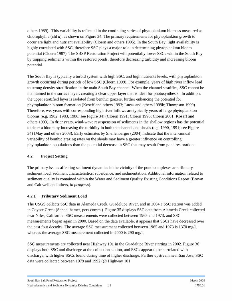
others 1989). This variability is reflected in the continuing series of phytoplankton biomass measured as chlorophyll a (chl a), as shown on Figure 34. The primary requirements for phytoplankton growth to occur are light and nutrient availability (Cloern and others 1995). In the South Bay, light availability is highly correlated with SSC, therefore SSC plays a major role in determining phytoplankton bloom potential (Cloern 1987). The SBSP Restoration Project will potentially lower SSCs within the South Bay by trapping sediments within the restored ponds, therefore decreasing turbidity and increasing bloom potential. The South Bay is typically a turbid system with high SSC, and high nutrients levels, with phytoplankton growth occurring during periods of low SSC (Cloern 1999). For example, years of high river inflow lead to strong density stratification in the main South Bay channel. When the channel stratifies, SSC cannot be maintained in the surface layer, creating a clear upper layer that is ideal for photosynthesis. In addition, the upper stratified layer is isolated from benthic grazers, further enhancing the potential for phytoplankton bloom formation (Koseff and others 1993; Lucas and others 1999b; Thompson 1999). Therefore, wet years with corresponding high river inflows are typically years of large phytoplankton blooms (e.g. 1982, 1983, 1986; see Figure 34) (Cloern 1991; Cloern 1996; Cloern 2001; Koseff and others 1993). In drier years, wind-wave resuspension of sediments in the shallow regions has the potential to deter a bloom by increasing the turbidity in both the channel and shoals (e.g. 1990, 1991; see Figure 34) (May and others 2003). Early estimates by Shellenbarger (2004) indicate that the inter-annual variability of benthic grazing rates on the shoals may have a greater influence on controlling phytoplankton populations than the potential decrease in SSC that may result from pond restoration. 4.2 Project Setting The primary issues affecting sediment dynamics in the vicinity of the pond complexes are tributary sediment load, sediment characteristics, subsidence, and sedimentation. Additional information related to sediment quality is contained within the Water and Sediment Quality Existing Conditions Report (Brown and Caldwell and others, in progress). 4.2.1 Tributary Sediment Load

The USGS collects SSC data in Alameda Creek, Guadelupe River, and in 2004 a SSC station was added in Coyote Creek (Schoellhamer, pers comm.). Figure 35 displays SSC data from Alameda Creek collected near Niles, California. SSC measurements were collected between 1965 and 1973, and SSC measurements began again in 2000. Based on the data available, it appears that SSCs have decreased over the past four decades. The average SSC measurement collected between 1965 and 1973 is 1370 mg/l, whereas the average SSC measurement collected in 2000 is 290 mg/l. SSC measurements are collected near Highway 101 in the Guadalupe River starting in 2002. Figure 36 displays both SSC and discharge at the collection station, and SSCs appear to be correlated with discharge, with higher SSCs found during time of higher discharge. Farther upstream near San Jose, SSC data were collected between 1979 and 1992 (@ Highway 101



Figure 37). As with the current measurements, higher SSCs typically coincide with time of high discharge. In February of 1980, peak flows of nearly 8000 cfs correspond with SSC values of approximately 800 mg/l. 4.2.2 Sediment Characteristics

Most of the salt ponds are composed of a mix of sand, silt, and clay deposited from the South Bay and the tributaries (U.S. Geological Survey 2004). In the Alviso complex, the ponds contain on average 38% sand, 36% silt, and 26% clay; the ponds in Eden Landing contain 38% sand, 39% silt, and 23% clay; and the Ravenswood ponds contain 55% sand, 32% silt, and 13% clay (U.S. Geological Survey 2004). This represents a marked difference from the area slough channels (e.g. Alviso, Artesian, Mud, and Guadalupe Slough) , which on average contain higher amounts of silt and clay (13% sand, 54% silt, and 33% clay) near the slough mouths (U.S. Geological Survey 2004). The sediments within the salt ponds and the shoals of the South Bay have experienced varying degrees of consolidation. Understanding the sediment bed characteristics will be an important aspect of restoration planning. Determining the sediment bed characteristics (i.e. critical shear stresses for erosion, bulk density, age, etc.) over the shoals and pond areas of the South Bay is listed as a Priority Data Gap in the Data Summary Report (PWA and others 2004a). 4.2.3 Pond Bottom Elevations and Subsidence

The existing pond bottoms reflect decades of subsidence, caused primarily by compaction through soil oxidation and groundwater withdrawal (Siegel and Bachand 2002). Soil oxidation and compaction occurs when marsh soils are drained. For ponds that are periodically drained as part of salt production, soil oxidation may have led to some subsidence. However, most South Bay salt ponds are normally flooded, and oxidation is not likely a significant factor. Groundwater withdrawals, on the other hand, have been well documented as a cause of considerable subsidence in the South Bay (Watson 2004), particularly between 1912 and 1969 when aquifer overdraft resulted in as much as 13 feet of subsidence with increasing severity towards the south. Subsidence is currently controlled by an integrated system of water imports, regulated pumping, and artificial recharge, which prevent the water table from reaching critical depths (Watson 2004). Rising groundwater level in the 1990s caused up to 5.1 mm ± 2.3 mm/yr in the Santa Clara Valley, although the currents rates of uplift are still much less significant that historic rates of subsidence (Watson 2004). Although the ponds themselves have subsided, un-diked tidal marshes in the South Bay were able to maintain their elevations relative to sea level rise and did not become submerged (Watson 2004). In fact, some areas that were once open water have converted to new marsh (H. T. Harvey & Associates 2002). The existing and expected future subsidence rates in the South Bay are listed as a priority Data Gap in the Data Summary Report (PWA and others 2004a). Additional information related to subsidence and vegetation colonization within the SBSP Restoration Project is contained within the Flood Management and Infrastructure Existing Conditions Report (PWA and others, in progress), and the Biology and Habitats Existing Conditions Report (H. T. Harvey & Associates and others, in progress).



Figure 38 shows the current pond bathymetry for the Eden Landing Complex and Figure 39 shows the pond bathymetry for the Alviso Complex, as measured in a recent survey by the USGS. The ponds shown without bathymetry were either too shallow or too filled with debris for the survey collection methods. The majority of the remaining pond bathymetry, along with the South Bay mudflats, will be determined using the LiDAR data collected by TerraPoint (2005) under contract to the California State Coastal Conservancy. This data is currently being processed for later review and inclusion in the SBSP Restoration Project. 4.2.4 Marsh Sedimentation

Sedimentation is important for raising mudflat areas and pond bottoms to elevations at which marsh vegetation can establish. The rate of estuarine sedimentation in natural and restored marshes depends on sediment supply in the water column, settling velocities, and the period of marsh inundation. Sediments are carried into a marsh and deposited on flood tides. The amount of sediment carried into the site depends on SSCs at the sediment supply source (e.g., the outboard mudflats) and the distance of the site from this source. Sedimentation rates will vary within a site, with the highest rates generally occurring nearest the breach and along the edges of the channels. The rate of sedimentation decreases as mudflats and marsh plains build in elevation and the period of tidal inundation decreases. Sedimentation rates can also be inhibited by waves and restricted tidal exchange. Consolidation occurs over time particularly as the mudflats rise within the tidal frame and are dewatered more frequently. Colonizing vegetation on accreting mudflats enhances sediment trapping and sedimentation rates. Measured sedimentation data are available from restored tidal marshes and dredged marinas in the South Bay. Sedimentation data were reviewed from the Cooley Landing Salt Pond Restoration (PWA 2004), Palo Alto Yacht Harbor (PWA 1987), Steven’s Creek Marsh restoration (Brown & Caldwell and others in progress), Alviso Marina (Ruth and Going Inc. and others 1980), and Warm Springs Marsh restoration (a.k.a. Coyote Creek Lagoon) (PWA and Phyllis Faber & Associates 2003). Sedimentation data were collected from Cargill Pond B-1 Marsh Restoration as part of this study to supplement data previously collected by Wetland Research Associates (2000). The locations of these restored marshes and dredged marinas are shown in Figure 40. Wind-wave conditions within these sites are not expected to significantly limit sedimentation rates. The sites all have full tidal connections to the Bay (i.e., a full tide range within the site). Cargill Pond B1 and Steven’s Creek Marsh were managed using water control structures prior to full tidal restoration. For these sites, only data collected after full tidal restoration occurred was included in the analysis described below. Sedimentation data from the above sites were analyzed using MARSH98. MARSH 98 is a simple estuarine sedimentation model developed by PWA from Krone’s (1987) method for simulating marsh elevations. Indicators of SSC were estimated for each site by calibrating MARSH 98 to the measured sedimentation data. This approach allows comparison of observed sedimentation rates, which were measured at different elevations in the tidal frame and vary depending on the corresponding period of inundation as well as the sediment supply.



MARSH 98 is based on the mass balance of suspended sediment, the frequency and duration of tidal inundation, the settling velocity of suspended sediments, and accumulation of deposited material. Input parameters to MARSH 98 are SSC index, bulk density of deposited inorganic material, tide series, and sea level rise. The model output is elevation over time. The SSC index is used as a calibration parameter to fit modeled sedimentation to measured sedimentation data. This index is characteristic of long-term average SSC and is useful for comparing sediment availability between sites or regions. Actual SSCs vary greatly in response to spring-neap tide cycles, seasonal changes in wind and rainfall patterns, and severe or El Niño storm events. Krone (1987) gives a dry bulk density of inorganic material of 560 mg/l for pickleweed marshes in the South Bay. As dry bulk density data from restored marsh deposits are not available, this value was selected for input to MARSH98. Tide series were developed for each site using a mean monthly tide series for the Presidio; tide height and time conversions for locations near each site available from NOAA tide predictions (National Oceanic & Atmospheric Administration 2005); and approximate conversions from the mean lower low water tidal datum to the National Geodetic Vertical Datum of 1929 (NGVD29) from Siegel and Bachand (2002), U.S. Army Corps of Engineers (1984), and National Oceanic & Atmospheric Administration (2005). The mean monthly tide series is a one-month-long tide series containing spring and neap tide cycles that is statistically equivalent to a longer-term (one year) tide series. Sea level rise was not included in the MARSH98 model runs because the amount of sea level rise and sensitivity of modeled sedimentation to sea level rise is negligible over the short monitoring periods. Table 5 contains the measured sedimentation data and estimated SSC index for each site. Figure 41 plots the measured data on MARSH98 sedimentation curves calibrated to the SSC indices. The results show that sediment availability, as represented by the SSC indices, is greatest for the far South Bay and decreases down-estuary. These patterns of marsh sedimentation are consistent with regional patterns of sediment transport in the South Bay (see Section 4.1.3). The results of the marsh sedimentation analysis indicate that the highest rates of marsh sedimentation are expected in the Alviso Complex, especially areas along Coyote Creek and Alviso Slough. The SSC index for the western part of the Alviso Complex is less than for Coyote Creek and Alviso Slough to the east. Sediment availability is lower for the Ravenswood and Eden Landing Complexes. Sediment availability for the Ravenswood Complex may be different than at Cooley Landing due to differences in wind exposure. Cooley Landing is sheltered from dominant and extreme wind directions, whereas the Ravenswood Complex is exposed to these winds. Further assessment of sedimentation in marsh areas and marinas to the north of the Ravenswood Complex may benefit future analyses. The time series of mudflat elevations available for Warm Springs and Stevens Creek suggest that significant consolidation occurred as the mudflats built up to intertidal elevations. Elevation gains at both sites stalled, or even turned negative (elevations decreased), as the mudflat surfaces reached approximately mean tide level. This phenomenon is likely a result of mudflat consolidation outpacing new surface deposition. As notes above, MARSH98 does not simulate consolidation. Table 5 – Measured sedimentation data and MARSH98 SSC indices Site Nearby Pond MARSH98 Measured Sedimentation Data



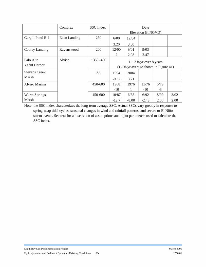
Complex SSC Index Date Elevation (ft NGVD)

6/00 12/04 Cargill Pond B-1 Eden Landing 250

3.20 3.50 12/00 9/01 9/03 Cooley Landing Ravenswood 200

2 2.08 2.47 Palo Alto Yacht Harbor

~350- 400 1 – 2 ft/yr over 8 years (1.5 ft/yr average shown in Figure 41)

1994 2004 Stevens Creek Marsh

350

-0.62 3.71 1968 1976 11/76 5/79 Alviso Marina 450-600 -10 1 -10 -3

10/87 6/88 6/92 8/99 3/02 Warm Springs Marsh

Alviso

450-600 -12.7 -8.00 -2.43 2.00 2.00

Note: the SSC index characterizes the long-term average SSC. Actual SSCs vary greatly in response to spring-neap tidal cycles, seasonal changes in wind and rainfall patterns, and severe or El Niño storm events. See text for a discussion of assumptions and input parameters used to calculate the SSC index.



5. REFERENCES

Alpers CN, Ayers SM, Domagalski JL, Slotton DG, Suchanek TH. Mercury and Methylmercury Concentration and Loads in the Cache Creek Watershed, California, January 2000 through May 2001, An Assessment of Ecological and Human Health Impacts of Mercury in the Bay-Delta Watershed, CALFED Bay-Delta Program.

Arnsberg AJ, Cole BE, Cloern JE. 1998. Studies of the San Francisco Bay, California Estuarine Ecosystem: Regional monitoring program results, 1998. U.S. Geological Survey Open-File Report 01-68. 217 p.

Atwater BF, Hedel CW, Helley EJ. 1977. Late Quaternary depositional history, Holocene sea-level changes, and vertical crustal movement in southern San Francisco Bay, CA. USGS Professional Paper 1014. 15 pp. p.

Baylosis JI, Edmunds JL, Cole BE, Cloern JE. 1997. Studies of the San Francisco Bay, California Estuarine Ecosystem: Pilot regional monitoring results, 1996. U.S. Geological Survey Open-File Report 97-598. 203 p.

Baylosis JI, Edmunds JL, Cole BE, Cloern JE. 1998. Studies of the San Francisco Bay, California Estuarine Ecosystem: Regional monitoring program results, 1997. U.S. Geological Survey Open-File Report 98-168. 194 p.

Bricker J. 2003. Bed drag coefficient variability under wind waves in a tidal estuary: field measurements and numerical modeling [PhD Thesis]. Stanford, CA: Stanford University. 161 p.

Brown & Caldwell, PWA, H. T. Harvey & Associates, GAIA Consulting I. Unpublished draft report, expected to be finalized in February 2005. Moffett Field Storm Water Retention Pond Tidal Restoration Feasibility Study. Prepared for NASA Ames Research Center.

Brown and Caldwell. 2004. Mercury Technical Memorandum, South Bay Salt Pond Restoration Project. San Francisco, CA.: Prepared for: California State Coastal Conservancy, U.S. Fish and Wildlife Service, California Department of Fish and Game.

Buchanan P. 1999. Specific conductance, water temperature, and water level data, San Francisco Bay, California, water year 1998. Interagency Ecological Program Newsletter 12(4):46-51.

Buchanan PA. 2003. Specific-conductance, water-temperature, and water-level data, San Francisco Bay, California, water years 2001-2002. Interagency Ecological Program Newsletter 16(4):25-30.

Buchanan PA, Ganju NK. 2002. Summary of suspended-sediment concentration data, San Francisco Bay, California, water year 2000. U.S. Geological Survey. Report nr 02-146.

Buchanan PA, Ruhl CA. 2000. Summary of suspended-solids concentration data, San Francisco Bay, California, water year 1998. U.S. Geological Survey. Report nr 00-88. 41 p.

Buchanan PA, Ruhl CA. 2001. Summary of suspended-solids concentration data, San Francisco Bay, California, water year 1999. U.S. Geological Survey. Report nr 01-100. 56 p.

Buchanan PA, Schoellhamer DH. 1998. Summary of suspended-solids concentration data in San Francisco Bay, California, water year 1996. U.S. Geological Survey. Report nr 98-175. 59 p.

Buchanan PA, Schoellhamer DH. 1999. Summary of suspended-solids concentration data in San Francisco Bay, California, water year 1997. U.S. Geological Survey. Report nr 99-189. 52 p.

Buchanan PA, Schoellhamer DH, Scheipline RC. 1996. Summary of sespended solids concetraion data, San Francisco Bay, California, water year 1994. Sacramento, CA: United States Geological Survey. Report nr OFR-95-776.

Cheng R, Casulli V. 1982. On lagrangian residual currents with applications in South San Francisco Bay, California. Water Resources Research 18(6):1652-1662.

Cheng RT, Casulli V, Gartner JW. 1993. Tidal, residual, intertidal mudflat (TRIM) model and its applications to San-Francisco Bay, California. Estuarine, Coastal, and Shelf Science 36(3):p235-280.

Cheng RT, Gartner JW. 1984. Tides, tidal, and residual currents in San Francisco Bay, California --Results of measurements, 1979-1980. USGS. Report nr 84-4339.



Cheng RT, Gartner JW. 1985. Harmonic Analysis of tides and tidal Currents in South San Francisco Bay, California. Estuarine, Coastal, and Shelf Science 21:p57-74.

Cheng RT, Smith LH. 1985. Tidal Hydraulics of San Francisco Bay and Estuary. Symposium II, Selenium and Agricultural Drainage: Implications for San Francisco Bay and the California Environment. Berkeley, California. p p132-150.

City of San Jose. 2004. Publications and research, http://www.ci.san-jose.ca.us/esd/pub_res.htm. City of San Jose.

Cloern J. 1987. Turbidity as a control on phytoplankton biomass and productivity in estuaries. Continental Shelf Research 7(11-12):1367-1381.

Cloern J. 1991. Tidal stirring and phytoplankton bloom dynamics in an estuary. Journal of Marine Research 49(1):203-221.

Cloern J. 1996. Phytoplankton bloom dynamics in coastal ecosystems: A review with some general lessons from sustained investigation of San Francisco Bay, California. Reviews of Geophysics 34(2):127-168.

Cloern J. 1999. The relative importance of light and nutrient limitation of phytoplankton growth: a simple index of coastal ecosystem sensitivity to nutrient enrichment. Aquatic Ecology 33:3-16.

Cloern J. 2001. Our evolving conceptual model of the coastal eutrophication problem. Marine Ecology-Progress Series 210:223-253.

Cloern J, Powell T, Huzzey L. 1989. Spatial and temporal variability in South San Francisco Bay (USA). 2. Temporal changes in salinity, suspended sediments, and phytoplankton biomass and productivity over tidal time scales. Estuarine, Coastal and Shelf Science 28(6):599-613.

Cloern JE, Grenz C, Lucas LV. 1995. An empirical model of the phytoplankton chlorophyll:carbon ratio - The conversion factor between productivity and growth rate. Limnology and Oceanography 40(7):1313-1321.

Cole B, Cloern J. 1987. An emperical-model for estimating phytoplankton productivity in estuaries. Marine Ecology-Progess Series 36(3):299-305.

Edmunds JL, Cole BE, Cloern JE, Caffrey JM, Jassby AD. 1995. Studies of the San Francisco Bay, California, Estuarine Ecosystem. Pilot Regional Monitoring Program Results, 1994. US Geological Survey. Report nr Open-File Report 95-378. 436 p.

Edmunds JL, Cole BE, Cloern JE, Dufford RG. 1997. Studies of the San Francisco Bay, California, Estuarine Ecosystem. Pilot Regional Monitoring Program Results, 1995. US Geological Survey. Report nr Open-File Report 97-15. 380 p.

Fischer HB, Lawrence GA. 1983. Currents in South San Francisco Bay. State Water Resources Control Board, California. Report nr UCB/HEL-83/01.

Fischer HB, List EJ, Koh RCY, Imberger J, Brooks NH. 1979. Mixing Inland and Coastal Water: Academic Press. 483 pp. p.

Foxgrover AC, Higgins SA, Ingraca MK, Jaffe BE, Smith RE. 2004. Deposition, erosion, and bathymetric change in South San Francisco Bay: 1858-1983.: U.S. Geologic Survey.

Gartner JW, Walters RA. 1986. Tidal and residual currents in South San Francisco Bay, California. Results of measurements 1981-1983. U.S. Geological Survey Open-File Report 86-4024. Menlo Park, CA.

Gilbert GK. 1917. Hydraulic mining debris in the Sierra Nevada USGS Professional Paper 105. U.S. Geologic Survey. 154 p.

Grenz C, Cloern J, Hager S, Cole B. 2000. Dynamics of nutrient cycling and related benthic nutrient and oxygen fluxes during a spring phytoplankton bloom in South San Francisco Bay (USA). Marine Ecology-Progress Series 197:67-80.

Grimm CK. 1931. Study of tidal currents and silt movements in the San Francisco Bay area with particular reference to the effect of a salt water barrier upon them. U.S. Army Corps of Engineers. Report nr Appendix D to House Document 191, 71st Congress, 3rd Edition.

Gross E. 1997. Numerical modeling of hydrodynamics and scalar transport in an estuary [PhD Thesis]. Stanford, CA: Stanford University. 331 p.



http://www.ci.san-jose.ca.us/esd/pub_res.htm

Gross E. 2003. Alviso Island Pond Breach Initial Stewardship Plan Study. South Bay Salt Ponds Initial Stewardship Plan, Draft Environmental Impact Report/Environmental Impact Statement, Technical Appendix K.: California Department of Fish and Game and U.S. Fish and Wildlife Service,.

Gross E, Koseff J, Monismith S. 1999. Three-dimensional salinity simulations of south San Francisco Bay. Journal of Hydraulic Engineering - ASCE 125(11):1199-1209.

Gunther A, Salop P, Bell D, Feng A, Wiegel J, Wood R. 2001. Initial Characterization of PCB, Mercury, and PAH Contamination in the Drainages of Western Alameda County, CA, http://www.cleanwaterprogram.com/publications_libraryResources.htm. The Alameda County Public Works Agency, Alameda Countywide Clean Water Program.

H. T. Harvey & Associates. 2002. Marsh Plant Associations of South San Francisco Bay: 2003 Comparative Study. San Jose, California: Prepared for City of San Jose. 78 p.

H. T. Harvey & Associates, PWA. 2005. Island Ponds (Ponds A19, A20, A21) Tidal Marsh Establishment Projections. Prepared for Santa Clara Valley Water District. Report nr PWA#1757.

Huzzey LM, Cloem JE, Powell TM. 1990. Episodic changes in lateral transport and phytoplankton distribution in south San Francisco Bay. Limnology & Oceanography 35(2):472-478.

Inagaki S. 2000. Effects of proposed San Francisco Airport runway extension on hydrodynamics and sediment transport in South San Francisco Bay [Engineers Thesis]. Stanford, CA: Stanford University. 98 p.

Jassby A, Koseff J, SG M. 1996. Processes underlying phytoplankton variability in San Francisco Bay. In: Hollibaugh JT, editor. San Francisco Bay: The Ecosystem. San Francisco: AAAS. p 325-349.

Koltermann CE, Gorelick SM. 1992. Paleoclimatic signature in terrestrial flood deposits. Science 256:1775-1782.

Koseff J, Holen J, Monismith S, Cloern J. 1993. Coupled effects of vertical mixing and benthic grazing on phytoplankton populations in shallow, turbid estuaries. Journal of Marine Research 51(4):843-868.

Krone OBa. 1992. Sediment Budget for San Francisco Bay. p 25 pp. Krone RB. 1962. Flume studies of the transport of sediment in estuarial shoaling processes. Berkeley,

CA: UC Berkeley. Krone RB. 1979. Sedimentation in the San Francisco Bay System. In: Conomos TJ, editor. San Francisco

Bay: The Urbanized Estuary. San Francisco, CA: Pacific Division, American Association for the Advancement of Science.

Krone RB. 1987. A Method for Simulating Historic Marsh Elevations. Presented at ASCE Specialty Conference, Coastal Sediments '87 New Orleans, LA:12-14.

Krone RB. 1996. Recent Sedimentation in the San Francisco Bay System. In: Hollibaugh JT, editor. San Francisco Bay: The Ecosystem: Pacific Division of the American Association for the Advancement of Science.

Lacy J, Schoellhamer D, Burau J. Suspended-solids flux at a shallow water site in South San Francisco Bay, California; 1996; Anaheim, CA.

Life Science. 2003. South Bay Salt Ponds Initial Stewardship Plan. Prepared for U.S. Fish and Wildlife Service and California Department of Fish and Game.

Life Science. 2004. South Bay Salt Ponds Initial Stewardship Project: Environmental Impact Report/Environmental Impact Statement. Prepared for U.S. Fish and Wildlife Service and California Department of Fish and Game.

Lucas L. 1997. A numerical investigation of coupled hydrodynamic and phytoplankton dynamics in shallow estuaries [PhD Thesis]. Stanford, CA: Stanford University.

Lucas L, Koseff J, Cloern J, Monismith S, Thompson J. 1999a. Processes governing phytoplankton blooms in estuaries. I: The local production-loss balance. Marine Ecology-Progress Series 187:1-15.



http://www.cleanwaterprogram.com/publications_libraryResources.htm

Lucas L, Koseff J, Monismith S, Cloern J, Thompson J. 1999b. Processes governing phytoplankton blooms in estuaries. II: The role of horizontal transport. Marine Ecology-Progress Series 187:17-30.

May C, Koseff J, Lucas L, Cloern J, Schoellhamer D. 2003. Effects of spatial and temporal variability of turbidity on phytoplankton blooms. Marine Ecology-Progress Series 254:111-128.

McDonald E, Cheng R. 1996. A numerical model of sediment transport applied to San Francisco Bay, CA. Journal of Marine Environmental Engineering 4:1-41.

McKee L, Ganju N, Schoellhammer D, Davis J, Yee D, Leatherbarrow J, Hoenicke R. 2002. Estimates of suspended-sediment flux entering San Francisco Bay from the Sacramento and San Joaquin Delta. San Francisco Estuary Insitutute. 28 p.

Moffatt & Nichol Engineers. 2005a. Hydrodynamic Modeling Tools and Techniques: South Bay Salt Pond Restoration Project. California State Coastal Conservancy. 42 pp. p.

Moffatt & Nichol Engineers. 2005b. Inventory of Water Conveyance Facilities: South Bay Salt Pond Restoration Project. California State Coastal Conservancy.

Moffatt & Nichol Engineers. 2005c. Summary of South San Francisco Bay Winter-Spring 2004 Interim Monitoring Data: South Bay Salt Pond Restoration Project. California State Coastal Conservancy. Report nr 5.

Monsen NE, Cloem JE, Lucas LV. 2002. A comment on the use of flushing time, residence time, and age as transport time scales. Limnol Oceanogr 47(5):1545-1553.

National Oceanic & Atmospheric Administration. Tides and Currents. NOAA/NOS Center for Operational Oceanographic Products and Services.

Ogden Beeman & Associates, Ray B. Krone & Associates. 1992. Sediment Budget for San Francisco Bay. Report nr Final report prepared for the SF District Corps of Engineers. 25 pp. p.

Powell M, Cloern J, Walters R. 1986. Phytoplankton spatial distribution in South San Francisco Bay: Mesoscale and small-scale variability. Estuarine Variability: Academic Press. p 369-383.

Powell T, Cloern J, Huzzey L. 1989. Spatial and temporal variability in South San Francisco Bay (USA). 1. Horizontal distributions of salinity, suspended sediments, and phytoplankton biomass and productivity. Estuarine Coastal and Shelf Science 28(6):583-597.

PWA. 1987. Hydrologic Factors in the Palo Alto Yacht Harbor Restoration. Report nr PWA#406. PWA. 2004. Cooley Landing Salt Pond Restoration Year-3 Monitoring Report. Prepared for Star-Link

Logistics, Inc., North Carolina. 24 plus appendices p. PWA, H. T. Harvey & Associates, Brown and Caldwell, EDAW. 2004a. Data Summary Report, South

Bay Salt Pond Restoration Project. San Jose, CA.: Prepared for: California State Coastal Conservancy, U.S. Fish and Wildlife Service, California Department of Fish and Game.

PWA, H. T. Harvey & Associates, EDAW, Brown and Caldwell. 2004b. Initial Opportunities and Constraints Summary Report, South Bay Salt Pond Restoration Project. San Francisco, CA.: Prepared for: California State Coastal Conservancy, U.S. Fish and Wildlife Service, California Department of Fish and Game.

PWA, Phyllis Faber & Associates. 2003. Monitoring the Evolution of Restored Tidal Marshes in San Francisco Bay: Physical and Vegetation Monitoring Data For Warm Springs, Muzzi, & China Camp Marshes from 1981 to 2003. Prepared for The Bay Institute. Report nr PWA#1575.

Ruhl CA, Schoellhamer DH. 2001. Time series of SSC, salinity, temperature, and total mercury concentration in San Francisco Bay during water year 1998: Regional Monitoring Program for Trace Substances contribution number 44. Richmond, California: San Francisco Estuary Institute.

Ruhl CA, Schoellhamer DH, Stumpf RP, Lindsay CL. 2001. Combined use of remote sensing and continuous monitoring to analyse the variability of suspended-sediment concentration in San Francisco Bay, California. Estuarine, Coastal and Shelf Science 53:801-812.

Ruth and Going Inc., Cooper-Clark Associates, Krone RB, Cheney MH. 1980. Causes of Sedimentation at Santa Clara County Marina, Alviso and Remedial Measures. Draft Report. Prepared for the County of Santa Clara.



Schemel LE. 1995. Measurements of salinity, temperature, and tides in South San Francisco Bay, California, at Dumbarton Bridge: 1990-1993 water years. US Geological Survey. Report nr Open-File Report 98-650.

Schemel LE. 1998. Salinity and temperature in South San Francisco Bay, California, at Dumbarton Bridge: Measurements from the 1995-1998 Water Years and comparisons with results from the 1990-1993 Water Years. US Geological Survey. Report nr Open-File Report 98-650.

Schoellhamer D. 1996. Factors affecting suspended-solids concentrations in South San Francisco Bay, California. Journal of Geophysical Research - Oceans 101(C5):12087-12095.

Schoellhamer DH. 2002. Variability of suspended-sediment concentration at tidal to annual time scales in San Francisco Bay, USA. Continental Shelf Research 22:1857-1866.

Schoellhamer DH. New findings on Bay sedimentation - discussing analysis of Bay Bridge SSC data, new sediment budget for the Bay, and turbidity maxima in the Bay; 2004 March 17, 2004.

Schoellhamer DH, Buchanan PA, Ganju NK. Ten years of continuous suspended-sediment concentration monitoring in San Francisco Bay and Delta; 2002 April 30 - May 2, 2002; Reno, Nevada.

Schoellhamer DH, Ganju NK, Gartner JW, Murrell MC, Wright SA. Seasonal and longitudinal homogeneity of suspended sediment in San Francisco Bay, California; 2003 September 14-18, 2003; Seattle, WA. Estuarine Research Federation.

Shellenbarger GG, Schoellhamer DH, Lionberger MA. 2004. A South San Francisco Bay Sediment Budget: Wetland Restoration and Potential Effects on Phytoplankton Blooms. ASLO-TOS 2004 Ocean Research Conference. Honolulu.

Siegel SW, Bachand PAM. 2002. Feasibility Analysis, South Bay Salt Pond Restoration. San Rafael, California: Wetlands and Water Resources. 228 p.

Smith BJ. Sedimentation in the San Francisco Bay system; 1965. US Dept. of Agriculture. Stoffer P, Gordon L. 2001. Geology and Natural History of the San Francisco Bay Area, A Field-Trip

Guidebook. U.S. Geological Survey. Report nr Bulletin 2188. TerraPoint. 2005. Project Report, USGS - South Bay Restoration Project. 33 p. Thompson B, Hoenicke R, Davis JA, Gunther A. 2000. An overview of contaminant-related issues

identified by monitoring in San Francisco Bay. Environmental Monitoring and Assessment 64(1):409-419.

Thompson JK. 1999. The effect of infaunal bivalve grazing on phytoplankton bloom development in South San Francisco Bay. PhD Thesis, Stanford University.

U.S. Army Corps of Engineers. 1954. A review of sedimentation. Report nr Appendix G of the Report to the Water Project Authority of the Sate of California Feasibility of Construction of Barriers in the San Francisco Bay System.

U.S. Army Corps of Engineers. 1984. San Francisco Bay Tidal Stage vs. Frequency Study. U.S. Geological Survey. 2004. Science Support for Salt Pond Restoration and Management: Short-term

Data Collection Needs, South Bay Salt Ponds Restoration Project Sediment Samples. United States Geological Survey (USGS).

U.S. Geological Survey. 2004a. Continuous Monitoring in the San Francisco Bay and Delta http://sfbay.wr.usgs.gov/access/Fixed_sta/. United States Geological Survey (USGS).

U.S. Geological Survey. 2004e. Surface Water Data for the USA: Monthly Streamflow Statistics http://nwis.waterdata.usgs.gov. US Geological Survey. Uncles RJ, Peterson DH. 1995. A computer model of long-term salinity in San Francisco Bay: sensitivity

to mixing and inflows. Environmental International 21(5):647-656. URS. 2002. Proposed SFO Runway Reconfiguration Project, Predicted changes in hydrodynamics,

sediment transport, water quality, and aquatic biotic communities associated with SFO runway reconfiguration. Alternative BX-6. Prepared for the City and County of San Francisco and the Federal Aviation Administration.

Walters RA. 1982. Low-Frequency Variations in Sea Level and Currents in South San Francisco Bay. Journal of Physical Oceanography 12: p658-668.



http://sfbay.wr.usgs.gov/access/Fixed_sta/

http://nwis.waterdata.usgs.gov/

Walters RA, Cheng RT, Conomos TJ. 1985. Time scales of circulation and mixing processes of San Francisco Bay waters. Hydrobiologia 129: p13-36.

Watson EB. 2004. Changing elevation, accretion, and tidal marsh plant assemblages in a south San Francisco Bay tidal marsh. Estuaries 27(4):684-696.

Weissmass G, Mount J, Fogg G. 2002. Glacially driven cycles in accumulation space and sequence stratigraphy of a stream-dominated alluvial fan, San Joaquin Valley, California, USA. Journal of Sedimentary Research 72(2):240-251.

Wetlands Research Associates. 2000. Annual Monitoring Report Preliminary Results Following Introduction of Full Tidal Conditions Year 5. San Rafael, CA: Prepared for: Cargill Salt Company for submission to: U.S. Army Corps of Engineers COE Permit # 19009E98. 24 p.

Wright SA, Schoellhamer DH. Trends in the sediment yield of the Sacramento River, 1957-2001; 2003 January 14-16, 2003; Sacramento, California. CALFED.

Wright SA, Schoellhamer DH. 2004. Trends in the Sediment Yield of the Sacramento River, California, 1957 - 2001. San Francisco Estuary and Watershed Science 2(2).

Yancey T, Lee J. 1972. Major heavy mineral assemblages and heavy mineral provinces of the central California coast region. Geological Society of America Bulletin 83:2099-2104.



6. LIST OF PREPARERS

The following PWA Team members assisted in preparation of this document: Kris May, PWA Nick Garrity, PWA Steve Crooks, PWA Michelle Orr, PWA Philip Williams, PWA Adam Parris, PWA Don Danmeier, PWA Source files for this report are located at PWA: \\orca\pwa\Projects\1720_SouthBay-Stage1\Task01_Alts_Devt\Existing_Conditions\Hydrology_and_Sediment\Hydrology_&_Sediment_v1.9.doc



\\orca\pwa\Projects\1720_SouthBay-Stage1\Task01_Alts_Devt\Existing_Conditions\Hydrology_and_Sediment\tidal_data\comparison_hourly2004.xls3/29/2005

-2.00

0.00

2.00

4.00

6.00

8.00

10.00

6/1/04 18:00 6/2/04 0:00 6/2/04 6:00 6/2/04 12:00 6/2/04 18:00 6/3/04 0:00 6/3/04 6:00

Tida

l Hei

ght (

ft, M

LLW

)

Dumbarton Bridge Redwood City San Mateo Bridge Oyster Point Hunters Point San Francisco

f i g u r e 2Source: http://co-ops.nos.noaa.gov/

South Bay Salt Pond Resotration ProjectTidal height variations within the South Bay

\\orca\pwa\Projects\1720_SouthBay-Stage1\Task01_Alts_Devt\Existing_Conditions\Hydrology_and_Sediment\tidal_data\2004_tides.xls 3/29/2005

Typical Daily Tidal Cycle at San Francisco (Station #9414290)

-2.00

0.00

2.00

4.00

6.00

8.00

6/1/04 18:00 6/2/04 0:00 6/2/04 6:00 6/2/04 12:00 6/2/04 18:00 6/3/04 0:00 6/3/04 6:00

Tida

l Hei

ght (

ft, M

LLW

)

MHHW

MLW

MLLW

MHW

Typically Monthly Tidal Cycle at San Francisco (Station 9414290)

-4

-2

0

2

4

6

8

6/1/04 6/6/04 6/11/04 6/16/04 6/21/04 6/26/04 7/1/04

Tida

l Hei

ght (

ft, M

LLW

)

South Bay Salt Pond Resotration ProjectTidal variability in San Francisco Bay

Neap Tide Neap Tide

Spring Tide Spring Tide


\\orca\pwa\Projects\1720_SouthBay-Stage1\Task01_Alts_Devt\Existing_Conditions\Hydrology_and_Sediment\tidal_data\2004_tides.xls 3/29/2005

Typical Annual Tidal Cycle at San Francisco (Station #9414290)

-3

-1

1

3

5

7

9

Jan-03 Mar-03 May-03 Jul-03 Sep-03 Nov-03 Jan-04

Tida

l Hei

ght (

ft, M

LLW

)


South Bay Salt Pond Resotration ProjectTypical annual tidal cycle

f igure 5

South Bay Salt Pond Restoration ProjectUSGS monitoring site locations

Source: Schoellhamer and Ruhl, 2001

PWA Ref# 1750.01

\\orca\pwa\Projects\1720_SouthBay-Stage1\Task01_Alts_Devt\Existing_Conditions\Hydrology_and_Sediment\USHS_monitoring_sites.doc

\\orca\pwa\Projects\1720_SouthBay-Stage1\Task01_Alts_Devt\Existing_Conditions\Hydrology_and_Sediment\delta_outflow\outflow_2.xls 3/29/2005

0

100000

200000

300000

400000

500000

600000

700000

1990 1992 1994 1996 1998 2000

Del

ta O

utflo

w (c

fs)

f i g u r e 6Source: http://www.iep.ca.gov/dayflow/output/index.html

South Bay Salt Pond Resotration ProjectDelta Outflow

f igure 7

South Bay Salt Pond Restoration ProjectBay Bridge near-surface and near-bottom salinity

Source: http://sfbay.wr.usgs.gov/access/Fixed_sta/

PWA Ref# 1750.01

\\orca\pwa\Projects\1720_SouthBay-Stage1\Task01_Alts_Devt\Existing_Conditions\Hydrology_and_Sediment\salinity_figures_2.doc

f igure 8

South Bay Salt Pond Restoration ProjectSan Mateo Bridge near-surface and near-bottom salinity


PWA Ref# 1750.01

\\orca\pwa\Projects\1720_SouthBay-Stage1\Task01_Alts_Devt\Existing_Conditions\Hydrology_and_Sediment\salinity_figures_2.doc

salinity.xls 3/29/05

0

10

20

30

40

1990 1992 1994 1996 1998 2000

10 years starting from 1/01/1990, decimal year

NE

AR

SU

RFA

CE

SA

LIN

ITY

f i g u r e 9Source: http://water.usgs.gov/pubs/wri/wri034005/

South Bay Salt Pond Resotration ProjectDumbarton Bridge near-surface salinity

\\orca\pwa\Projects\1720_SouthBay-Stage1\Task01_Alts_Devt\Existing_Conditions\Hydrology_and_Sediment\channel_marker_17_data\cm17 winter 2004.mod.xls 3/29/2005

Channel Marker 17 SalinityWinter 2004

9

11

13

15

17

19

21

23

25

27

29

1-Dec 21-Dec 10-Jan 30-Jan 19-Feb 11-Mar 31-Mar 20-Apr 10-May

Salin

ity (P

SU)

Near surfaceNear bottom

f i g u r e 10Source: Schoellhamer and Shellenbarger, pers. comm

South Bay Salt Pond Resotration ProjectChannel marker 17 near-surface and near-bottom salinity

\\orca\pwa\Projects\1720_SouthBay-Stage1\Task01_Alts_Devt\Existing_Conditions\Hydrology_and_Sediment\salinity\salinity3.xls 3/29/2005

0

10

20

30

40

1990 1992 1994 1996 1998 2000

Dum

barto

n Br

idge

South Bay Salt Pond Resotration ProjectDelta outflow and South Bay near-surface salinity

0

10

20

30

40

1990 1992 1994 1996 1998 2000

San

Mat

eo B

ridge

0

10

20

30

40

1990 1992 1994 1996 1998 2000

Pie

r 24

/ Bay

Brid

ge

0.E+00

2.E+05

4.E+05

6.E+05

1990 1991 1992 1993 1994 1995 1996 1997 1998 1999 2000

Del

ta O

utflo

w (c

fs)

f i g u r e 11Source: http://sfbay.wr.usgs.gov/access/Fixed_sta/

Depth in meters

Salinity

(psu)

Cruise date: February 6, 1991

Salinity

(psu)


f igure 12

South Bay Salt Pond Restoration Project Longitudinal salinity profiles from a dry year (1991) and wet year (1998)

Source: http://sfbay.wr.usgs.gov/access/wqdata/

PWA Ref# 1750.01

P:\Projects\1720_SouthBay-Stage1\Task01_Alts_Devt\Existing_Conditions\Hydrology_and_Sediment\salinity_figures_2.doc 3/29/2005

(m)

Salinity

(psu)

Cruise date: November 6, 1997

Cruise date: January 6, 1998





f igure 13

South Bay Salt Pond Restoration ProjectLongitudinal salinity profiles during an El Niño winter (1998)


PWA Ref# 1750.01

P:\Projects\1720_SouthBay-Stage1\Task01_Alts_Devt\Existing_Conditions\Hydrology_and_Sediment\salinity_figures_2.doc

D

D

DD

#

#

#

#

#

LEGEND

#Top and Bottom CTD

#Top CTD

DWater Level

Deep BayFully TidalFully Tidal BaylandShallow Bay

Map datum and projection: NAD83, UTM, Zone 10NMap Data: USGS DOQQ (aerial photos), Moffatt & Nichol (locations)

±

SBSP Restoration ProjectSBSP Restoration ProjectFigure 14 -- Moffat & Nichol Instrument Locations

0 5,000 10,0002,500 Feet

Dumbarton Bridge

Stevens Creek(downstream)

Stevens Creek(upstream)

Alviso Slough

Railroad Bridge

0 1,500 3,000750 Meters

Coyote Hills Slough

Ravenswood Slough

Guadalupe Slough

Power Tower

\\orca\pwa\Projects\1720_SouthBay-Stage1\Task01_Alts_Devt\Existing_Conditions\Hydrology_and_Sediment\streamflow_data\streamflow.xls 3/29/2005

USGS Daily Streamflow Station 11172175Coyote Creek @ Highway 237

0

200

400

600

800

1000

1200

1400

Jan-99 Jul-99 Jan-00 Jul-00 Jan-01 Jul-01 Jan-02 Jul-02 Jan-03 Jul-03

Dis

char

ge (c

fs)

f i g u r e 15Source: http://nwis.waterdata.usgs.gov/usa/nwis/discharge/?site_no=111172175

South Bay Salt Pond Resotration ProjectDaily streamflow measurements for Coyote Creek @ Highway 237


USGS Daily Streamflow Station 11169025Guadalupe River @ Highway 101

0

200

400

600

800

1000

1200

1400

1600

1800

2000

May

-02

Jun-

02

Jul-0

2

Aug-

02

Sep-

02

Oct

-02

Nov

-02

Dec

-02

Jan-

03

Feb-

03

Mar

-03

Apr-

03

May

-03

Jun-

03

Jul-0

3

Aug-

03

Sep-

03

Dis

char

ge (c

fs)

South Bay Salt Pond Resotration ProjectDaily streamflow measurements for Guadalupe River @ Highway 101



USGS Daily Streamflow Station 11179000 Alameda Creek near Niles

0

5000

10000

15000

20000

25000

1900 1910 1920 1930 1940 1950 1960 1970 1980 1990 2000

Dis

char

ge (c

fs)


South Bay Salt Pond Resotration ProjectDaily streamflow measurements for Alameda Creek near Niles


USGS Daily Streamflow Station 11180700Alameda Creek Flood Control Channel @ Union City

0

2000

4000

6000

8000

10000

12000

14000

16000

1960 1965 1970 1975 1980 1985 1990 1995 2000 2005

Dis

char

ge (c

fs)


South Bay Salt Pond Resotration ProjectDaily streamflow measurements for Alameda Creek Flood Control Channel @ Union City


USGS Daily Streamflow Station 11164500San Francisquito Creek @ Stanford University

0

500

1000

1500

2000

2500

3000

1930 1940 1950 1960 1970 1980 1990 2000

Dis

char

ge (c

fs)


South Bay Salt Pond Resotration ProjectDaily streamflow measurements for San Francisquito Creek @ Stanford University


USGS Daily Streamflow Station 11166000Matadero Creek @ Palo Alto

0

50

100

150

200

250

300

350

400

450

500

1950 1955 1960 1965 1970 1975 1980 1985 1990 1995 2000

Dis

char

ge (c

fs)


South Bay Salt Pond Resotration ProjectDaily streamflow measurements for Matadero Creek @ Palo Alto

f igure 25

South Bay Salt Pond Restoration ProjectBay Bridge mid-depth and near-bottom SSC


PWA Ref# 1750.01

\\orca\pwa\Projects\1720_SouthBay-Stage1\Task01_Alts_Devt\Existing_Conditions\Hydrology_and_Sediment\sediment_figures_2.doc

f igure 26

South Bay Salt Pond Restoration ProjectSan Mateo Bridge mid-depth and near-bottom SSC


PWA Ref# 1750.01


f igure 27

South Bay Salt Pond Restoration ProjectDumbarton Bridge mid-depth and near-bottom SSC


PWA Ref# 1750.01


f igure 28

South Bay Salt Pond Restoration ProjectChannel Marker 17 mid-depth and near-bottom SSC


PWA Ref# 1750.01


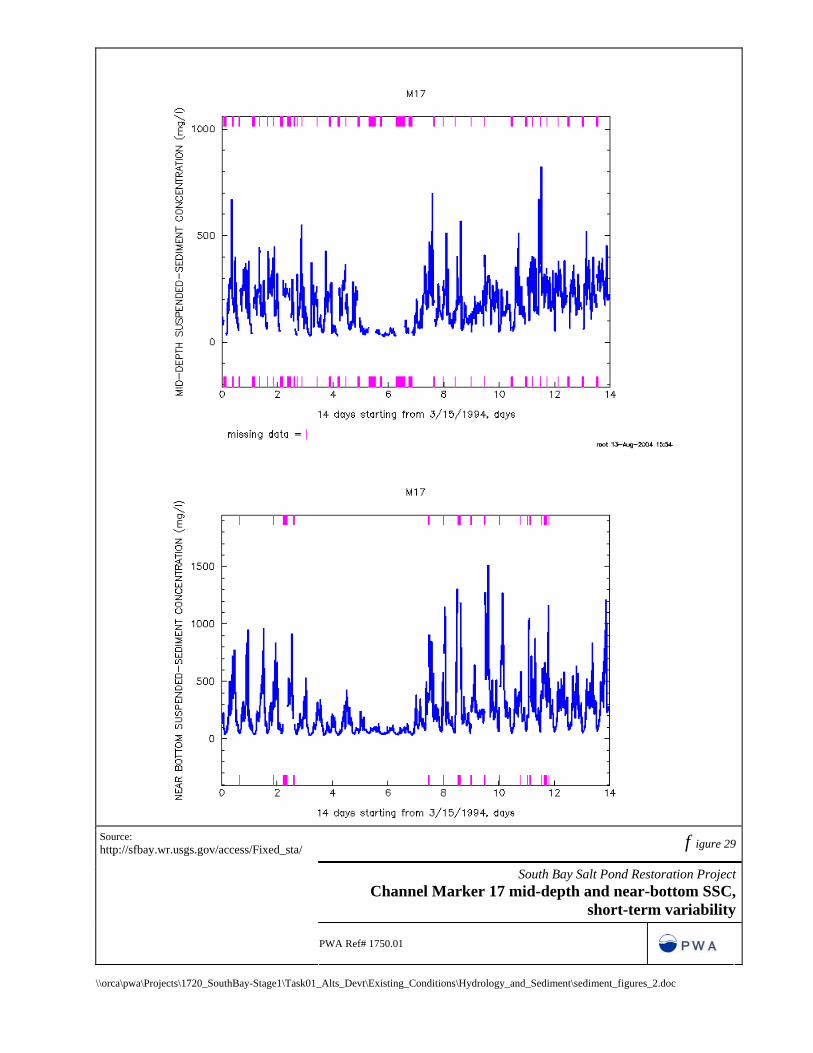
f igure 29

South Bay Salt Pond Restoration ProjectChannel Marker 17 mid-depth and near-bottom SSC,

short-term variability


PWA Ref# 1750.01


(m)

Suspended Particulate Matter

(mg l-1)



(mg l-1)



(mg l-1)



(mg l-1)



(mg l-1)



(mg l-1)


f igure 30

South Bay Salt Pond Restoration ProjectLongitudinal suspended particulate matter profiles during an

El Niño winter (1998)


PWA Ref# 1750.01

P:\Projects\1720_SouthBay-Stage1\Task01_Alts_Devt\Existing_Conditions\Hydrology_and_Sediment\sediment_figures_long.doc 3/30/2005

(m)

Phytoplankton Biomass (Chl a)

(mg m-3)



(mg m-3)



(mg m-3)



(mg m-3)



(mg m-3)



(mg m-3)


f igure 31

South Bay Salt Pond Restoration ProjectLongitudinal phytoplankton biomass profiles during an El

Niño winter (1998)


PWA Ref# 1750.01


(m)


(mg l-1)

Cruise date: April 9, 1998


(mg l-1)



(mg l-1)

Cruise date: May 19, 1998


(mg l-1)

Cruise date: August 11, 1998


(mg l-1)

Cruise date: September 1, 1998


(mg l-1)


f igure 32

South Bay Salt Pond Restoration ProjectLongitudinal suspended particulate matter profiles during

summer (1998)


PWA Ref# 1750.01


(m)


(mg m-3)



(mg m-3)



(mg m-3)

Cruise date: May 19, 1998


(mg m-3)

Cruise date: August 11, 1998


(mg m-3)

Cruise date: September 1, 1998


(mg m-3)


f igure 33

South Bay Salt Pond Restoration ProjectLongitudinal phytoplankton biomass profiles during summer

(1998)


PWA Ref# 1750.01


f igure 34

South Bay Salt Pond Restoration ProjectLong-term variability in spring bloom magnitude


PWA Ref# 1750.01

\\orca\pwa\Projects\1720_SouthBay-Stage1\Task01_Alts_Devt\Existing_Conditions\Hydrology_and_Sediment\sediment_figures_2.doc 3/30/2005


USGS Water Quality Samples Station 11179000Alameda Creek near Niles

0

1000

2000

3000

4000

5000

6000

7000

8000

1965 1970 1975 1980 1985 1990 1995 2000

Susp

ende

d Se

dim

ent C

once

ntra

tions

(mg/

l)

f i g u r e 35Source: http://nwis.waterdata.usgs.gov/usa/nwis/qwdata/?site_no=111179000

South Bay Salt Pond Resotration ProjectSuspended sediment concentrations in Alameda Creek near Niles


USGS Water Quality Samples Station 11169025Guadalupe River at Highway 101

0

200

400

600

800

1000

1200

1400

1600

11/1/2002 12/1/2002 1/1/2003 2/1/2003 3/1/2003 4/1/2003 5/1/2003 6/1/2003 7/1/2003

Dis

char

ge (c

fs)

0

50

100

150

200

250

300

350

400

450

SSC

(mg/

l)

DischargeSSC

South Bay Salt Pond Resotration ProjectSuspended sediment concentrations in Guadalupe River at Highway 101



USGS Water Quality Samples Station 11169000Guadalupe River @ San Jose

0

1000

2000

3000

4000

5000

6000

7000

8000

9000

1979 1980 1981 1982 1983 1984 1985 1986 1987 1988 1989 1990 1991 1992

Dis

char

ge (c

fs)

0

100

200

300

400

500

600

700

800

900

SSC

(mg/

l)

Discharge

SSC


South Bay Salt Pond Resotration ProjectSuspended sediment concentrations in Guadalupe River @ San Jose

LEGENDSedimentation Monitoring LocationDeep BayFully TidalFully Tidal BaylandShallow Bay

Map datum and projection: NAD83, UTM, Zone 10NMap Data: USGS DOQQ (aerial photos)

±

SBSP Restoration ProjectSBSP Restoration ProjectFigure 40 -- Locations of Sedimentation Monitoring

0 5,000 10,0002,500 Feet

Cooley Landing

Palo Alto Yatch Harbor

Stevens Creek Marsh

Alviso Marina

Warms Springs

0 1,500 3,000750 Meters

Cargill Pond B-1

f igure 41

South Bay Salt Pond Restoration Project Measured sedimentation data and Marsh98 sedimentation curves

Note: The time scale is not fixed to a particular date and measured data for a given site is not plotted relative to other sites Source: Krone 1987; PWA 1987, 2003, and 2004; Brown and Caldwell and others 2004; Ruth and others, 980

PWA Ref# 1750.01

\\orca\pwa\Projects\1720_SouthBay-Stage1\Task01_Alts_Devt\Existing_Conditions\Hydrology_and_Sediment\Marsh98.doc 3/30/2005

table of contents 3. hydrodynamics 8 · table of contents page 1. executive summary 2 2....

Documents