TABLE OF CONTENTS

I. Introduction .............................................................................................................. 1

II. Understanding Technical Analysis .................................................................... 2

III. Separating Myth from Reality ............................................................................. 4

IV. Understanding the Importance of World Capital Flows ............................. 6

V. The Shape of a Wave .............................................................................................. 8

VI. Phase Transition .................................................................................................. 11

VII. Understanding Time ........................................................................................... 13

VIII. Timing Models ...................................................................................................... 16

IX. Bifurcation Models and the Science of Chaos .............................................. 18

X. Volatility Models .................................................................................................. 20

XI. Forecast Arrays ..................................................................................................... 21

XII. The Reversal System ........................................................................................... 26

XIII. How to Use the Indicating Ranges .................................................................. 29

XIV. Conclusion .............................................................................................................. 32

1

I. Introduction

This manual describes the Models & Methodologies employed by Princeton Economics to

interpret financial markets across the global economy. Princeton Economics employs a

completely different school of innovative thinking based on a non-subjective interpretation

of market and economic movement, which is essential in understanding the development

of the world economy and financial markets.

At Princeton Economics, we have created the first AI database (Socrates) capable of tracking capital flows on an international basis. To compile our database, we spent decades tracking the monetary history of the world, beginning with the earliest known forms of currency. We then created a system capable of building knowledge upon the accomplishments and failures of the past. Socrates considers all potential economic and

social variables by gathering data on everything from stocks, bonds, interest rates, and commodities to political trends, wars, and civil unrest. Socrates monitors nearly every currency in circulation to grasp a truly global perspective of the global economy. Most importantly, Socrates generates analyses without human intervention. This ensures that our analyses are non-subjective by removing the bias of personal observation.

If you are familiar with trading, this manual will resurface knowledge you may have

acquired while helping you to identify different dimensions of market activity that you

should focus on. Some of our terms may seem familiar, but our application will surprise

you. Once you understand how to interpret our detailed charts, they will act as your

personal roadmap to the markets.

To trade successfully you must have conviction in your belief, and that can only be

accomplished by acquiring a “feel” for the market. Never trade blindly. You must always

agree with what you are doing. That “feel” will be essential to surviving your own trading

decisions. Our methods can produce extraordinary results, but the value that one obtains is

directly dependent on one’s understanding of the terminology and methodology.

2

II. Understanding Technical Analysis

By definition, technical analysis refers to the study of past market price activity to

determine future price activity. When used in isolation to determine market patterns,

technical analysis is subjective and produces different results depending on whom is doing

the analysis. Perhaps the greatest threat to forecasting lies in the Observer Effect, which

states that the observer subconsciously inserts his or her own biases into the analysis, thus

altering the results. For this reason, Princeton Economics does not employ Fibonacci

Timing, Elliot Wave, Kondratieff Wave, or other similar models. Although price can be

determined using forms of technical analysis, measuring only the shape of a wave

dismisses the importance of time.

We are embarking on a road of analysis that is not subjective and is qualified with specific

dates to separate the observer from affecting the outcome of the analysis. This is the

primary goal. We utilize technical analysis as a confirmation tool for providing a visual

method of ascertaining market performance. Additionally, we look to technical analysis to

provide targets in price for support and resistance.

Princeton Economics also employs the use of cyclical analysis, which by definition is the

analysis of a time series that isolates regular rhythmic patterns of oscillation.

The three primary dimensions of market and economic movement are (1) time, (2) price,

and (3) volatility. However, a fourth dimension exists: interrelationships. Fundamental

analysis aims to reduce things to a specific cause and effect, but that is not reality.

Interrelationships and interconnectivity on a global scale are what really matters. For

example, a company’s earnings may be seen as bullish domestically, yet bearish

internationally. Within this realm, the fundamental approach must be global in nature and

never isolated to purely domestic trends.

At Princeton Economics, we use a method called International Capital Flow Analysis that

conforms to quantitative standards by monitoring the interactions across major world

economies which enables us to obtain consistent long-term forecasts.

Once you abandon the most commonly accepted maxims about why the markets move in

one direction versus another, you can begin to understand the actual trends that are

driving the world capital markets.

3

III. Separating Myth from Reality

There are many myths surrounding the markets that adversely affect the economy on a

global scale. Investors and government decision makers alike perpetuate these myths. To

understand how markets function, it is crucial to separate myth from reality. Below are a

few examples of common economic myths:

Myth: Short-selling causes panic declines.

Throughout history, whenever the stock market crashes, the majority blame short

positions for causing the panic. This has been the root cause of government investigations

during every panic.

Reality: A short position in stocks is created by borrowing stock and then selling it on the

market. Therefore, every short position actually results in a long position. The first is the

long position from whom the short borrows; the second is the long position created by the

person who bought the stock from the short seller. So at any given time, short positions are

outnumbered 2:1 in share markets, assuming that 100% of all outstanding stock was

originally borrowed.

In reality, short positions typically only account for a small percentage of total outstanding

positions. Therefore, it is impossible for short positions to outnumber long positions. This

only becomes possible in the instance of unlimited naked short selling, but that has never

happened.

In futures, two players must balance every contract: one long and one short. Therefore, in

commodities short positions can (at best) only match long positions. Even during the most

bearish moments, short positions will never outnumber long positions.

Myth: Interest rates provide an incentive to buy or sell stocks, bonds, and real estate at the

expense of all other stimuli.

Reality: Interest rates rise during bull markets and decline in bear markets. There is no

empirical evidence to support the idea that lowering interest rates will stimulate the

economy. In fact, lowering the interest rate reduces the income of those who have cash.

People will not borrow, even at 1%, if they do not see a profit. Interest rates always decline

during a depression, often creating the incentive to invest overseas. When capital cannot

earn money domestically, it then begins to migrate overseas. Lowering interest rates will

not stimulate the economy without a perceived opportunity to invest.

Myth: If a nation raises its base interest rate, the currency will rise because international

capital will be attracted by a greater return.

Reality: The problem that emerges is the lack of depth in this crude form of analysis.

Nothing takes place without reason; it is always, without exception, the combination of

numerous trends.

4

The inconsistent relationship of interest rates to the value of any currency is the result of a

plethora of factors that contribute to the underlying confidence of a nation and the ultimate

value of its currency. If interest rates were the only determining factor in the preeminent

value of a currency, then everyone would be running to places like Argentina where

interest rates rose to 300% per month or to Europe in the midst of a debt crisis.

The myths of interest rates and their effect within the global economy are by no means

one-dimensional. If high interest rates alone attract capital, then why do interest rates rise

when capital flees? Think of it akin to a loan shark: if the bank does not accept your credit,

then you turn to a loan shark at a much higher rate. Capital follows a bell curve and is

attracted to higher rates to a certain point. Once capital becomes frightened, it flees, and

interest rates begin to rise exponentially as confidence collapses. Interest rates also rise

exponentially when the value of the currency collapses in value. No relationship remains

linear; it will typically change direction following a bell curve.

Myth: When interest rates rise, stock prices decline, and when interest rates decline, stock

prices rise.

Reality: It would be wonderful if the stock market could be simplified to such a childish

rule. Surely if this were true, each and every reader would be a billionaire by now. There

are countless examples throughout history that say otherwise.

Myth: Stock prices can be determined by looking at bond prices, and vice versa.

Reality: What really counts in the relationship between stocks and bonds is none other than

confidence, which swings cyclically back and forth between these two instruments. Only

when all things remain equal do we find that stocks and bonds trade together in synchrony.

Whenever the underlying confidence is shook in one sector and not the other, huge

historical divergences occur. Cyclical trends are not restricted to a single market. Spread

traders know firsthand that huge divergences occur between any two given instruments.

Nothing remains constant; everything within the global economy vibrates with oscillating

trends back and forth. Vast long-term trends exist in every aspect from capital flows to

unemployment.

Myth: Central Banks can buy back government bonds to inject cash into the system to

stimulate the economy.

Reality: This myth assumes that domestic investors solely hold bonds. If foreign investors

hold bonds, as is the case for around 40% of all sovereign debt, then buying back the bonds

will result in exported cash and will not result in economic stimulation.

Conclusion: The danger presented by these types of market myths exposes the fallacy of

fundamental analysis. As mentioned earlier, fundamental analysis aims to reduce the

complexity of the world to a single cause and effect. We live in a Complex Adaptive

5

Dynamic System where everything is truly connected on a global scale. We cannot simply

reduce such a complex system to a single cause and effect.

Stocks and bonds swing with confidence, as people will not buy or sell without it. Although

many would argue that confidence is some sort of nebulous element that is impossible to

survey, the best method of determining confidence is the ultimate survey of all time —

market price movement. If you monitor market price movement and world capital trends,

you can gain a true sense of confidence in the underlying economy. When confidence

collapses, capital flees.

History always repeats, but it is very difficult (if not impossible) to find a point in time

when history has repeated precisely in the same manner throughout all economic sectors

simultaneously. What does tend to repeat are the overall trends toward oscillating

divergences and interrelationships.

There is a lot more to analyzing the global market than simply analyzing stock prices in

isolation. The secrets to major oscillations will not be revealed until we begin to analyze

and correlate the results on a global scale in conjunction with the major structural changes.

6

IV. Understanding the Importance of World Capital Flows

Man has desperately tried to predict the future since the dawn of time, gazing into the

heavens to observe the movement of stars, summoning soothsayers, mystics, psychics, and

even guidance from the patterns of tea leaves. He has studied the movements of planets,

comets, and even the flight of the owl. However, no matter what methods man has tried, his

attempts to pull back the curtain have never provided that infallible key to reveal the

mysteries that lie beyond the threshold of the future.

In this age of modern wisdom, we look back upon our forefathers as perhaps silly and

superstitious beings who ran around chucking spears and rocks at one another. The Age of

Enlightenment put aside prejudices of perception and progress returned to every field,

except economics, which was biased from its beginning in moral philosophy. Instead of

observing how it functioned, economics descended into the depths of prejudice as man set

out to discover how it operated in an attempt to alter the very way it functioned.

Unfortunately, prejudice has plagued economics for far too long. Many economists seek to

change “what is” into what they believe “should be”, thereby reducing the science of

economics to nothing more than a corrupt political social movement.

Understanding the nature of our global economy is not that difficult once we abandon

unrealistic social dreams of creating utopia and begin observing how it functions without

trying to interfere. The seemingly chaotic random behavior of our economy is due to the

enormous amount of complex variables that determine the outcome. A small change in

even one variable can result in dramatic changes within the overall global pattern.

An example from nature can be seen in the work of ecologists studying rainforests. Science

has come to understand that man cannot create a rainforest by merely planting a group of

trees and plants. There are millions of species of bacteria, insects, animals, plants, etc. that

interact to form a balance within nature. Man cannot duplicate such a complex system due

to his lack of knowledge concerning such a wealth of intricate variables interacting with

one another to produce the final balanced system.

Another problem for man in grasping a full understanding of market and economic

behavior lies in his conscious thought process. In our natural state, our mind processes and

records data in a nonlinear fashion. For example, when we meet someone special, perhaps

in a restaurant, our subconscious mind records the music and setting of the moment. The

subconscious mind quietly observes what the other person is wearing, the color of the

tablecloth, the flicker of the candlelight, the background music, etc. The conscious mind

observes the conversation at hand. Months or even years later, if we hear or see one of

those stimuli, our mind suddenly retrieves the experience and consciously relives the

event, right down to the twinkle of the candlelight. Economic and market behavior is quite

similar to the operation of our mind. There are numerous hidden variables within the

7

equation that produces the end result. Consciously, we focus on only a small fraction of

those variables involved and then desperately try to reduce every event to a single cause.

For example, we may pay attention to something like unemployment and its influence on

interest rates. We then try to interpret and pass judgement as to what the trend will be,

based upon a handful of fundamental relationships. Inevitably, such analysis proves

incorrect due to the lack of attention paid to the wealth of other variables. In financial

analysis, we ignore the actual process of collecting knowledge by continually trying to

reduce the entire fate or the world into a few simplistic relationships.

As famed economist Adam Smith mentioned in his Wealth of Nations, we all act according

to our own self-interests. Today this is magnified due to currencies becoming far more

visible on a global scale. Percentage swings of even 40% in two years have become much

more commonplace. Only a global model that filters in all key economic data along with

free market movements that includes everything from bonds and stocks to wheat and

aluminum, can hope to ascertain the trend.

The test of a real bull or bear market is one rising or falling on a global scale that is not

limited purely to one’s domestic currency perspective. What can appear to be bullish in

local currency can look dramatically different in international currency. Currency has

become everything and it is crucial to understand capital flows. Global trends are the result

of smaller trends emerging from every economy around the world. The trends in

international capital are set in motion by the forces of taxation, inflation, financial security,

foreign exchange, labor costs, geopolitics, and of course meddling politicians. There are

some minor influences as well, such as interest rate differentials. Nevertheless, capital is

continually flowing from one economy to the next in search of profit and/or financial

stability. This is nothing new as capital has been global for a very long time. There was even

the Silk Road between the West and East that dates back to the Stone Age.

8

V. The Shape of a Wave

There are two primary types of cyclical wave formations: transverse and longitudinal. Our computer models further divide these waves between fixed cycles and cyclical activity determined entirely by the computer.

Empirical (hardwired) transverse frequencies of a fixed duration display both short and long-term frequencies. The longitudinal wave is far more complex and dynamic in frequency, which fluctuate in duration. These are entirely ascertained by the computer on its own without predetermining the frequencies.

One of the great misconceptions in cycle theory is the notion that cycles unfold in a purely

symmetrical wave formation that is transverse in structure. This is simply not true, as we

will explore. There are also longitudinal wave structures where there is no symmetrical

distance between peaks. Both the Kondratieff Wave and Samuel Benner’s Wave structure

are longitudinal in nature. Perhaps instinctively, Benner understood cyclical shapes and

9

thus saw the repetitive patterns. Kondratieff merely identified three cyclical waves of

varying duration (wavelengths) and failed to address repetitive patterns.

Another fallacy that has prevented many from understanding cyclical movements has been

the concept of efficient markets adhering to some mysterious equilibrium that forms a

magical balancing act, such as the idea of supply and demand, existing inherently within the

system. The idea of equilibrium is like drawing a center line in the path of the swinging

pendulum. It is not the center line that provides the attraction and driving force of the

pendulum, rather it is always the two extreme forces on either side. There is no state of

perfect equilibrium acting as some mysterious driving force, nor is there an efficient center

force that the economy aims to achieve.

Unlike Kondratieff, Benner saw an inherent tendency for waves to build in intensity. His

wave broke down as a repetitive pattern of 18, 29, and 16-year intervals that built in

intensity to a 54-year wave structure. What he saw was the volatility. For this reason, the

shape of a wave is not a nice balanced structure.

The Economic Confidence Model, developed by Princeton Economic Intl. Chairman and

renowned economist Martin Armstrong, is a wave structure that builds in intensity through

six individual waves of 8.6 years that form a major wave of 51.6 years, which in turn builds

up once again into a 309.6-year structure. There is a fractal nature to this wave structure.

Additionally, it incorporates events that appear to come from nowhere, such as a rogue

wave of combined force in the ocean. It is by no means a one-dimensional bell curve. The

shape of the wave structure is vital to understand.

10

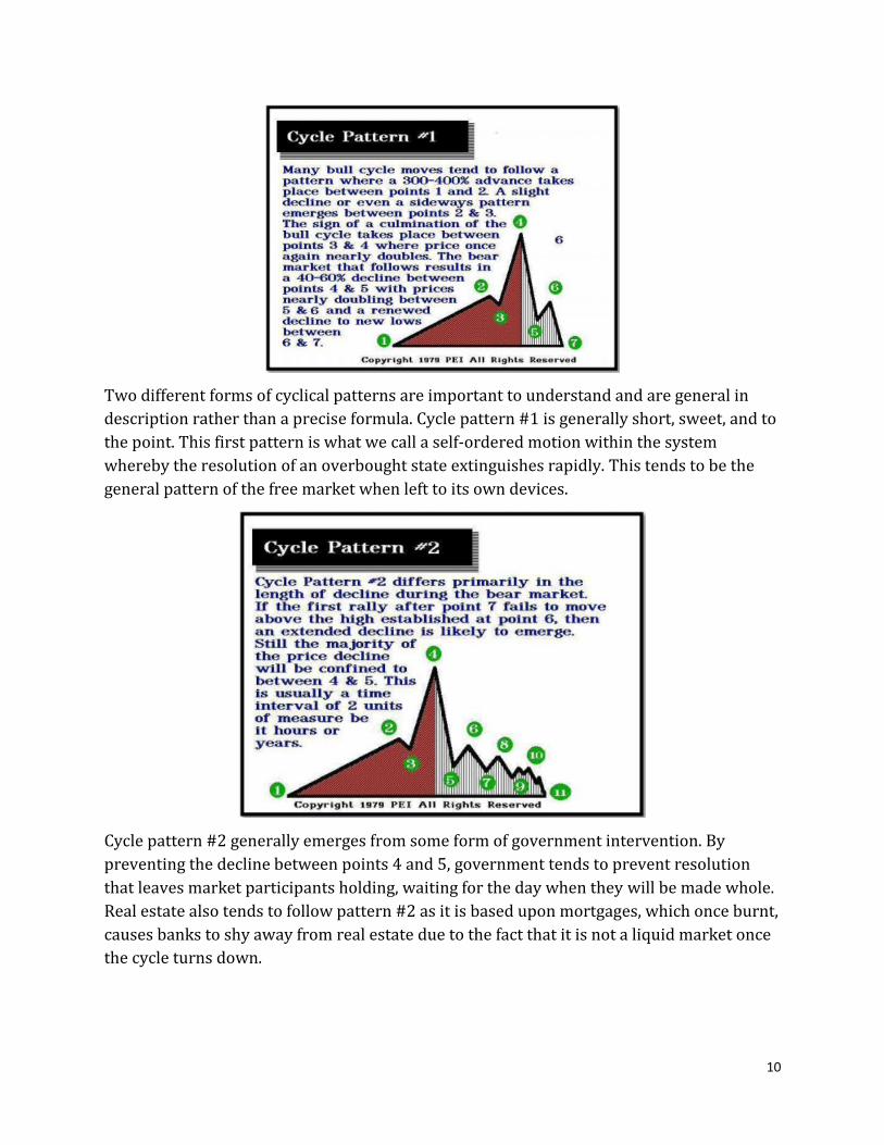
Two different forms of cyclical patterns are important to understand and are general in

description rather than a precise formula. Cycle pattern #1 is generally short, sweet, and to

the point. This first pattern is what we call a self-ordered motion within the system

whereby the resolution of an overbought state extinguishes rapidly. This tends to be the

general pattern of the free market when left to its own devices.

Cycle pattern #2 generally emerges from some form of government intervention. By

preventing the decline between points 4 and 5, government tends to prevent resolution

that leaves market participants holding, waiting for the day when they will be made whole.

Real estate also tends to follow pattern #2 as it is based upon mortgages, which once burnt,

causes banks to shy away from real estate due to the fact that it is not a liquid market once

the cycle turns down.

11

VI. Phase Transition

In physics, a physical system exists called a Phase Transition that crosses the boundary

between two changes in its properties in a fundamental way. For example, we can create a

Phase Transition by boiling water and moving from water to a gas. In simpler terms, a

Phase Transition changes in state from one form to another. Whatever exists in physical

systems also exists within the realm of economics for we may be biological organisms, but

there is no exception to the laws of physics. In the markets, the Phase Transition explains

abrupt movements in price. We can track the bullish and bearish consensus and see how it

moves between the two extremes. A Phase Transition accounts for the change between the

two extremes. However, this is by no means a linear progression. It very much follows the

same general course as boiling water.

At the nucleate boiling point, we see the

characteristic of bubbles on the heated

surface, which rise from discrete points on

a surface that is not uniform, and whose

temperature is only slightly above the

temperature of the liquid. Normally, the

number of nucleation irregular surface

points increases when the surface

temperature increases.

The next stage is the transition boiling

point, defined as the “unstable” boiling

point. This occurs at surface temperatures

between the maximum attainable in

nucleate and the minimum attainable in the final film boiling stage. This becomes the most

chaotic stage in the process. The formation of bubbles in a heated liquid is a complex

physical process, which often involves cavitation and acoustic effects, such as the hiss a

kettle makes before the water boils with bubbles forming on the surface.

The final film phase, also known as the Leidenfrost effect, occurs when the surface heating

the liquid is significantly hotter than the liquid, which causes a thin layer of vapor with low

thermal conductivity to insulate the surface. You can see this if you heat a skillet and then

sprinkle drops of water on it. When the skillet’s temperature exceeds the Leidenfrost point,

the water beads will move across the skillet. This actually causes the water beads to take

longer to evaporate opposed to being at a temperature above boiling but below

Leidenfrost’s point.

A Phase Transition accomplishes the same end game in physics as it does in economics. For

example, we can move back and forth from a bearish state to a neutral state where bulls

and bears tug back and forth to either state. The two extremes mark the dramatic

12

conviction that swings of the opposite force covers them, causing the Phase Transition to

unfold. This is not a normal bearish or bullish state, rather it is a compressed state of time

that convinces the majority within the marketplace to switch sides.

Understanding the Phase Transition is critical to understanding how to trade. The greatest

amount of gain and loss is accomplished in the shortest amount of time. So like a surfer

waiting in the ocean to ride the perfect wave, we must accomplish the same goal.

13

VII. Understanding Time

Using timing models to enhance your investment or corporate strategy may take some

getting used to. On one hand, large portfolios become unmanageable without a sense of

time. However, if there is no understanding of time, then you must take a loss for all you

can do is buy and hold. If you do not have a concept of time, you will lose everything after a

Phase Transition. You need to know when changes in trend will appear and begin to shift

direction in advance of the event unfolding. You cannot turn a battle ship on a dime, and

therefore time is essential when it comes to managing large portfolios.

Technical analysis is excellent for providing resistance and support targets, but trying to

ascertain the future unfolding based upon subjective analysis is not very reliable. All forms

of subjective analysis are open to interpretation, in which lies the problem.

Many assume that forecasts concerning time may possibly be accurate in the short-term,

but they remain skeptical about long-term timing forecasts. Many argue that major political

events cannot possibly be predicted in advance. To the contrary, such events would not

take place unless the economic condition had been in a steep decline. Computers cannot

predict what type of revolution will unfold as a result of a collapsing economy, but they can

predict when some sort of political change will take place due to economic pressures. Since

the dawn of civilization, no revolution has ever taken place unless man was first

economically deprived. Time is something that is quantifiable as everything has a cycle.

Contrary to popular belief, quantitative long-term timing forecasts actually display a higher

level of accuracy than the short-term. Long-term trends are set in motion by a combination

of forces, and these forces cannot turn around on a dime. Short-term trends involve a lot of

noise. People can become excited and falsely believe that the trend is changing, rushing in

where only fools would go. The trend fails and suddenly they bail out, causing the market

to revert back to the longer-term trend. The short-term is highly volatile; the long-term

trend is actually easier to predict than the short-term noise.

The critical aspect about time is that it is truly fractal in its construction. There are

numerous timing frequencies in a single market created by the many minor trends from a

variety of different investment strategies. We have found that long-term frequencies

always overpower short-term frequencies. Therefore, an 8-week cycle producing a low will

be overpowered by a 20-week cycle due to produce a high at the same time. One could say

that the 8-week cycle inverted or cancelled out by the stronger 20-week cycle. As this

process of long-term cycles dominating the short-term occurs, one begins to realize that

long-term cycles are more reliable than the short-term because they are far more difficult

to change.

14

The driving force behind the cycle is always

two opposing forces. Like a pendulum, these

driving forces act as a self-propelling

mechanism. There are two main groups in

markets (bulls and bears) just as there are

two main groups on politics (left and right).

Between these two hardcore groups exists a

flexible group who change their minds and

act independently. This group provides the

swing basis that adds the cycle to everything.

Since mankind is composed of individuals,

there are many different minor trends

within the collective whole. We can predict

the statistical direction, but we cannot

predict which individual trends will take up each side. It is far easier to predict the

collective sum of many small individual trends within the whole.

The cyclical process is how all forms of energy move. It is how light moves, sound, and even

electricity. The attraction of two opposite forces creates a self-propelling mechanism that

operates according to economic entropy, which is the measure of driving forces (energy) as

it is expended and is no longer available to continue to drive the cycle in that direction.

Once the bullish energy is expended, then the attractive force in the opposite direction

(bearish) overpowers the remaining bullish force and compels the cycle to then change

direction to the bearish attractor. This self-perpetuating endless cycle of life drives the

entire mechanism.

This is why shorts are vital because when they are wrong they have to buy, which adds to

the direction of the bullish trend. When the market collapses, only the short player has the

courage to stand up and buy in the middle of a panic, providing desperately needed

liquidity. Outlawing short positions is always the first step in a panic decline and is the best

way to ensure a further decline.

15

There are intraday traders who buy and sell numerous times within the course of a daily

session. These traders usually do not hold positions overnight. Therefore, even if the

overall trend is down, many of these people can be found on the long side of the market

intraday. They bring liquidity to the market, adding confidence at many times to embattled

longs. This helps to create cycles even within the intraday price movements.

Timing models are capable of providing the points in time when a high or low will unfold.

We refer to these points as Turning Points. They do not predict whether we will see a

specific event (high or low), but they can predict whether a certain event will materialize at

a given moment in time. Turning Points are simply concerned with time and how long a

trend will last. There are many different trends taking place at any moment in the internal

market as well as the interconnectivity influences from a full gambit of related and

unrelated markets on a global scale. Therefore, a local cycle producing a high can (1) cancel

out entirely by a larger counter-trend wave, or (2) invert by these same external forces.

This becomes the Superposition Principle that is either (A) a Constructive Inference that

causes the wave to magnify, or (B) a Destructive Inference that causes the local wave to

cancel out or invert.

Timing models are best suited to identify when a change in trend will unfold on short-term

price activity, but they do not always forecast whether that change in trend will leave

behind a specific high or low since there can be either a Cycle Inversion or Cycle

Cancellation due to the Superposition Principle. However, it becomes obvious that if a

market is declining and moving into a Turning Point, then that Turning Point will most

likely produce a low instead of a high. Computer models can predict the ideal periods

where a high or low will unfold, but this takes tremendous computing power.

The long-term rarely undergoes a Cycle Inversion or Cycle Cancellation, which tends to

indicate that at the lower echelons of time the influences are much more numerous. As we

graduate up the scale in time, the numerous individual trends combine to produce larger

waves and the complex composite does not allow for alterations so easily.

16

VIII. Timing Models

There are three primary methodologies to cyclical analysis, each with numerous layers of

inherent complexity.

1.) Composite Timing Models (Longitudinal Cyclical Waves)

2.) Empirical Timing Models (Transverse Cyclical Waves)

3.) Trading Timing Models (Differential Cyclical Waves)

i. Composite Timing Models

Composite Timing Models are longitudinal cyclical waves that expand and contract with no

definitive fixed duration between each wave. Composite Timing Models tend to repeat in a

broader overall group pattern.

For example, one wave may be 13 days, the next 34 days, followed by another 17-day cycle,

and finishing with an 8-day cycle. This may generate a pattern of 72 days, which then repeats.

This type of cyclical activity is addressed through Composite Timing Models, as they are the

result of a harmonic mix of many other timing elements. Composite frequencies form from

cyclical frequencies within the same market and external influences from other markets

across the globe.

ii. Empirical Timing Models

Transverse wave structures with fixed length timing frequencies also exist within a market

that is symmetrical in shape. We call this our Empirical Timing Model, meaning they are

“fixed” in wavelength.

For example, gold has historically had an 8-week cycle. At times, because of the

Superposition Principle, this cycle will undergo Destructive Inference and fail to produce a

Turning Point. This can cause the cycle to appear longitudinal in construction, yet it remains

very much transverse.

A fixed length cycle of 8 weeks may produce a high and low precisely every 8 weeks or for a

brief period in time. This cycle may suddenly disappear if it becomes overpowered by a

longer timing frequency from monthly, quarterly, or even yearly levels of activity within the

same market or influenced by interconnectivity of other market trends. After a few apparent

failures, this 8-week cycle will suddenly reappear exactly on target as if nothing had

happened. This fixed length cycle never changes in duration. When it stops working, it is only

because a frequency of greater importance is taking control. The greater force may be from

within the same market or the result of global interrelationships.

Empirical Models are very important timing elements. Just because a particular timing

frequency may appear successful on a few occasions does not guarantee its validity. Each

timing frequency employed in our Empirical Models has been historically tested as far back

17

as possible under all possible conditions. A frequency is only valid if it is consistent during a

bull and bear market. The majority of mistakes made by analysts are caused by the use of

timing models that have not been tested in both bull and bear markets.

iii. Trading Timing Models

Our Trading Timing Models are concerned solely with the nominal differences between bull

and bear market frequencies and traits. Our turning points generated by this model reflect

the statistical differences between these opposing trends without consideration of various

timing frequencies or intermarket relationships. The model specifically states what the

expected events should be (high or low) at a particular time interval. Unlike the other two

previously mentioned models, Trading Timing Models offer a union of time and direction,

and thus enable the user to qualify the forecast. Consequently, our Trading Timing Models

can offer a completely independent view as to what to expect.

Since trends become clearer during violent price action, this tool performs best during panics

in either direction. The periods when this pool provides a lower degree of accuracy is during

quiet non-trading periods. These are periods when both forces are about equal and tend to

cancel each other out.

This model recognizes that each market and sector has its own unique frequency. For

example, agricultural stocks are greatly influences by weather, crops, plating cycles, etc. and

thus are highly prone to greater volatility than one would find in other commodities, bonds,

or stocks.

18

IX. Bifurcation Models and the Science of Chaos

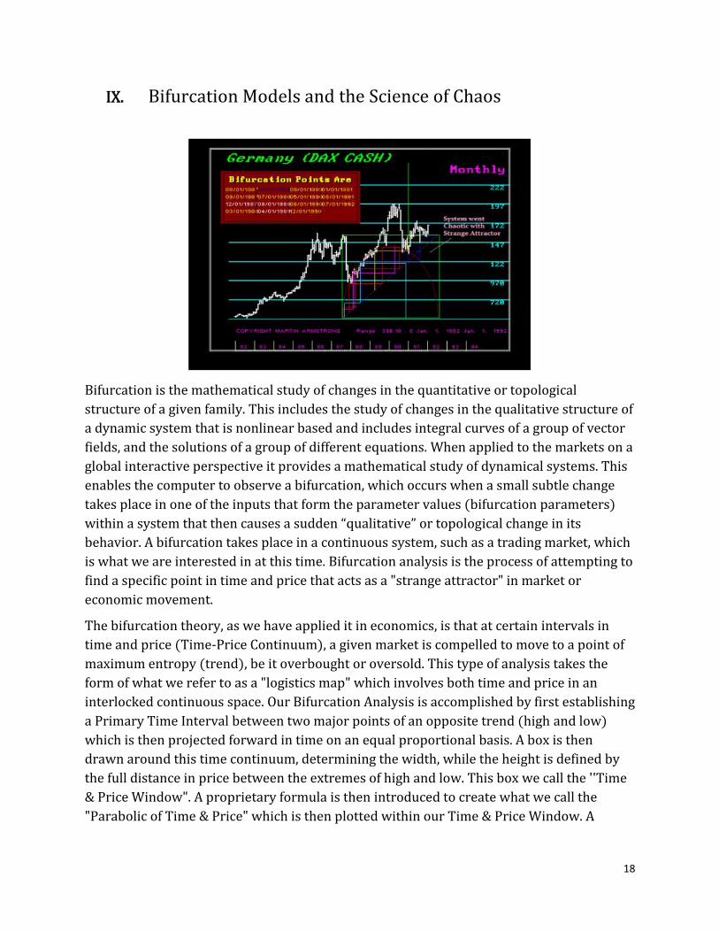
Bifurcation is the mathematical study of changes in the quantitative or topological

structure of a given family. This includes the study of changes in the qualitative structure of

a dynamic system that is nonlinear based and includes integral curves of a group of vector

fields, and the solutions of a group of different equations. When applied to the markets on a

global interactive perspective it provides a mathematical study of dynamical systems. This

enables the computer to observe a bifurcation, which occurs when a small subtle change

takes place in one of the inputs that form the parameter values (bifurcation parameters)

within a system that then causes a sudden “qualitative” or topological change in its

behavior. A bifurcation takes place in a continuous system, such as a trading market, which

is what we are interested in at this time. Bifurcation analysis is the process of attempting to

find a specific point in time and price that acts as a "strange attractor" in market or

economic movement.

The bifurcation theory, as we have applied it in economics, is that at certain intervals in

time and price (Time-Price Continuum), a given market is compelled to move to a point of

maximum entropy (trend), be it overbought or oversold. This type of analysis takes the

form of what we refer to as a "logistics map" which involves both time and price in an

interlocked continuous space. Our Bifurcation Analysis is accomplished by first establishing

a Primary Time Interval between two major points of an opposite trend (high and low)

which is then projected forward in time on an equal proportional basis. A box is then

drawn around this time continuum, determining the width, while the height is defined by

the full distance in price between the extremes of high and low. This box we call the ''Time

& Price Window". A proprietary formula is then introduced to create what we call the

"Parabolic of Time & Price" which is then plotted within our Time & Price Window. A

19

diagonal is then drawn from the lower left corner to the upper right corner. Once this

framework is established, the bifurcation plot begins.

Each time the bifurcation plot turns vertically, we obtain a time projection. All horizontal

plots offer a price projection. Extremely well behaved markets will contain this plot

between the diagonal and the parabolic. Occasionally, a strong strange attractor will appear

around the juncture of the diagonal and the parabolic, which will be evident by the plot

forming a box around this area. Very chaotic markets will show the plot suddenly breaking

out of the confining area between the parabolic and the diagonal.

The time and price targets derived from a bifurcation plot will often line up with targets

derived by cyclical and technical models, even though there is no similarity between these

methodologies. At other times, any other form of analysis cannot determine the targets

highlighted through our bifurcation plots. The purpose of our Bifurcation Model is to

determine whether or not there will be any major strange attractors in the future that seem

to help pinpoint major changes in trend. This can be very helpful in warning about

dramatic changes in trend. We use this model mainly as a confirmation tool rather than an

exclusive tool by itself. However, we do interface this model with that of our timing models

to help filter out which timing targets will be stronger than others. The Bifurcation Model

has been one of our most astonishing discoveries. It is purely a tool of chaos and by no

means is this within the realm of linear thinking. The Bifurcation Model is our window in to

the deep crevasses of a fully integrated dynamic nonlinear system.

20

X. Volatility Models

Volatility Models provide an indication as to when a change in the current volatility trend

will take place. Unlike timing, volatility is only concerned with percentage movements; it is

not concerned with direction or whether a high or low has formed within the market. The

model reflects "turning points" but in volatility. Thus, the low in volatility might form on

the highest bar while the high in volatility could unfold on the lowest bar. Our computer

employs 14 different models to measure volatility. However, we use three main models to

measure volatility:

1.) Internal Rate of Volatility

The Internal Rate of Volatility measures solely on a trading basis (i.e. a day, week, month,

quarter, or a year). This focuses on the percentage price movement between the high and

low strictly for that session.

2.) Closing Rate of Volatility

The Closing Rate of Volatility measures the close of the previous session to the close of the

current session.

3.) Overnight Volatility

Overnight Volatility measures the between the close of the previous day and the opening

day of the trading session.

By design, our Volatility Models accomplish a unique view of the markets that is typically

overlooked in other forms of analysis.

21

XI. Forecast Arrays

Forecast Arrays provide a quick graphical representation of a number of independent

forecasting models. This tool allows the user to quickly see when our computer models are

looking for ideal highs or lows, in addition to important changes in volatility.

Each model includes numerous variations, with some going as high as having 72 separate

models. Each model is plotted on an individual bar graph that increases with each timing

model and targets a specific period of time.

The plots within each model provide a guide as to where a Turning Point in price or

volatility should unfold. With the exception of the Trading Cycle indicator, each model is

designed to only provide an indication of when the market trend will change at a specific

point in time. The greater the number of individual timing frequencies that converge

during a specific time period, the greater the amplitude. Therefore, the tallest bar reflects

the greatest number of independent targets.

1.) Composite

The top bar on our Forecast Array provides the Composite, which is the combination of all

models converged to provide a good perspective of important future dates. Each separate

model from timing to volatility is taken as a sum of the bar graphs directly beneath it.

2.) Composite II

22

The second bar on our Forecast Array is the Composite II Model, which represents a

longitudinal timing model that expands and contracts through time. The cyclical frequencies are based upon the computer’s interpretation of the market’s cyclical pattern.

3.) Empirical

The third bar on our Forecast Array is the Empirical Model, which represents a transverse

form of cyclical frequency analysis. These frequencies are of fixed durations that have been

determined manually through decades of research. Additionally, these frequencies are

unique to each market.

4.) Long-Term

The fourth bar on our Forecast Array is the Long-Term Model, which represents a transverse form of cyclical frequency analysis. This model is typically three times the duration of the normal Empirical Timing Model. For example, if the Empirical Model represents a frequency that occurs every 16 weeks, then the Long-Term model will represent a frequency of approximately 48 weeks. Additionally, the frequencies are unique to each market.

5.) Trading Cycle

The fifth bar on our Forecast Array is the Trading Cycle, which represents a transverse form of cyclical frequency analysis. The Trading Cycle Model is color coordinated: green signals ideal highs, red signals ideal lows, and yellow signals a convergence in the cycles from both highs and lows appearing at the same time.

The Trading Timing Model offers a union of time and direction that enables the user to determine when a high or low is likely to occur. However, it is not guaranteed as cycles can be subjected to Destructive Interference under the Superposition Principle.

Bullish and bearish markets have empirical nominal durations that last specific time units (days, weeks, months, years):

Bullish: 7-11-14-21 time units Bearish: 2-3-5-6-10-12-18 time units

Bullish trading cycles are measured from a low and bearish trading cycles are measured from a high. The Trading Cycles Model quantifies the bullish and bearish predictions that fall on a particular time unit.

23

For example, the chart above shows how the cycles are counted; for brevity time unit 18 was ignored.

Time Unit #11 has three cycles that converge: two bullish and one bearish. Since they are of opposite market directions, a yellow bar is used as indication.

Based on the above data, the Trading Cycles array will appear as follows:

Bars appearing in green indicate an ideal time for highs, red indicates an ideal time for

lows, and yellow indicates a projection for a high and a low during the same time interval. When multiple cycles converge on a particular day, the bar will be larger. When two opposite cycles converge, the bar will appear in yellow.

6.) Most Active High

The sixth bar on our Forecast Array is the Most Active High, which represents a transverse form of cyclical analysis. These frequencies are generated exclusively from highs to highs and are different for each market.

7.) Alpha Cycle

The seventh bar on our Forecast Array is the Alpha Cycle, which represents a transverse

form of cyclical frequency analysis. The Alpha Cycle is generated strictly by analyzing high

to high. The data array bar increases or decreases in size depending on the number of

independent frequencies that converge on the same time interval. Additionally, the

frequency of the Alpha Cycle is different for each market.

24

8.) Most Active Low

The eighth bar on our Forecast Array is the Most Active Low, which represents a transverse

form of cyclical analysis. This model often signals that a turning point is in place. These

frequencies are generated exclusively from lows to lows and are different for each market.

9.) Beta Cycle

The ninth bar on our Forecast Array is the Beta Cycle, which represents a transverse form

of cyclical analysis. Opposite of the Alpha Cycle, the Beta Cycle Model is generated solely by

analyzing from low to low. The data array bar increases or decreases in size depending on

the number of independent frequencies that converge on same time interval. Additionally,

the frequency of the Beta Cycle is different for each market.

10.) Directional Change Model

The tenth bar on our Forecast Array is the Directional Change Model, which represents

Directional Changes and notes the point where a market begins to make a decisive move.

Unlike a Turning Point, the Directional Change targets do not need to be the actual high or

low.

For example, it is possible to find the intraday high or low take place 1 to 3 time units (days, weeks, months, etc.) preceding the Directional Change target. On a weekly level, the actual high might form on Wednesday while the market moves sideways within a narrow trading band until the Directional Change comes into play, perhaps in the following week.

During periods of high volatility, it is more common to find the Turning Point and Directional Change converge during the same time period. This normally occurs when a market is making a spike low or high.

11.) Panic Cycle

The eleventh bar on our Forecast Array represents the Panic Cycle Model. The Panic Cycle model represents whether an abrupt move is about to occur within the market. A Panic Cycle differs from a Turning Point or a Directional Change as it reflects neither a high nor a low and it is not the beginning of a change in trend.

25

Instead, a Panic Cycle more often than not is an outside reversals or just a capitulation. The

model reflects greater price movement that can be dramatic in one direction or an outside reversal exceeding the previous session high and penetrating its low.

12.) Internal Volatility

The twelfth bar on our Forecast Array represents our Internal Volatility Model that we discussed in the last section. Volatility Models provide an indication as to when a change in the current volatility trend will take place. Unlike timing, volatility is only concerned with percentage movement. This model is not concerned with direction nor whether a high or low has formed within the market. The model reflects "turning points" but in volatility.

Thus, the low in volatility might form on the highest bar while the high in volatility could unfold on the lowest bar.

As mentioned, the Internal Rate of Volatility measures solely on a trading basis (i.e. a day,

week, month, quarter, or a year). This focuses on the percentage price movement between

the high and low strictly for that session.

13.) Overnight Volatility

The final bar on our Forecast Array measures the Overnight Volatility. As mentioned,

Overnight Volatility measures the between the close of the previous day and the opening

day of the trading session.

26

XII. The Reversal System

In any market or economic statistic, there is some point that if crossed marks the beginning of a change in trend. These specific price levels exist in time series and can be thought of as key pressure points. They reflect the invisible inflection point related to entropy. Elected Reversal Points signal to the user whether they should buy or sell in a particular market. The election of the first Reversal Point indicates that a move to the second reversal is likely. An election of the second Reversal Point signifies that a move to the third point is probable

and so on.

Reversal Points are generated each time a market or economic statistic produces a new isolated high or low on an intraday or closing basis. Reversals Points are classified into four categories: Immediate, Major, Intermediate, or Minor depending upon the importance of the particular high or low.

1.) Immediate Reversal Points are generated from a reaction high or low that appears within a short-term trend. Bullish trends are generated from a low, while bearish trends are generated from a high.

2.) Major Reversal Points are generated from the highest highs or lowest lows within a given time series.

3.) Intermediate Reversal Points are generated from a high or low that appears within a long-term trend.

4.) Minor Reversal Points are generated from a reaction high or low that appears within a short-term trend.

Each of these four Reversal Points classifies the current trend by Immediate, Short, Intermediate, and Long-Term. Only when all four reversals are elected do we consider there

27

to be an important shift in trend. During extremely narrow sideways congested patterns, it

is best to avoid the reversals generated from every minor temporary high and low within the trading range and focus on the intermediate reversals.

Reversals that are generated from highs or lows are also differentiated into “Bullish” or “Bearish” reversals:

i.) Bearish Reversals are generated from a high. If the market should close below the Reversal Point, then the uptrend will reverse into a bearish or declining trend.

ii.) Bullish Reversals are generated from a low. If the If the market should close above the Reversal Point, then the downtrend will reverse into a bullish or increasing trend.

A reversal cannot be elected if the market closes precisely on it. In the case of a Bullish

Reversal, a successful election requires the markets to close above the reversal. Whereas in the case of a Bearish Reversal, an election requires that the closing is below the reversal.

Experienced traders can use Reversal Points for the opposite of their intended use. For example, a trader could place an order to buy against a Bearish Reversal with a protective stop just below.

Sometimes two or more of the Reversal Points generated from the high or low will be the same number or may be separated by a single basis point. When the election of these types of reversals occur, it signals an abrupt change in trend. These reversals are known as Double, Triple, or Quadruple Reversal Points:

A.) Double Reversal Points are generated twice by the same high or low. Historically,

double Reversal Points occur a few times during the course of a year on a daily level and once every two or three years on a weekly level. At very major highs and lows, it is normal to generate a Double Reversal on a monthly or weekly price level or higher.

B.) Triple Reversal Points are generated three times by the same high or low. Triple Reversal Points are extremely rare and have only occurred twice: once in gold in 1976 and once in the U.S. Treasury Bond futures in 1989.

C.) Quadruple Reversal Points are generated by the same high or low are the same. A Quadruple Reversal Point has only been elected once in history in the 1929 U.S. Stock Market.

Reversal Points can only be elected on a closing basis. For example, if gold was $1000.00 and a bullish reversal was $1001.00, the reversal would not be elected unless the closing price was greater than $1001.00.

Reversals are generated on all levels of price activity from daily to yearly. Daily Reversals are elected on a daily closing basis. However, in each case the next level of price activity will override the signal of a lower price level. Therefore, a Weekly Reversal will override

28

that of a daily when it is the last trading session of that particular week. Monthly Reversals

will override both Daily and Weekly Reversals on the last trading day of the month. A daily or weekly closing below a Monthly Reversal during the course of a month does not constitute an election of the Monthly Reversal. The election of Weekly, Monthly, Quarterly, and Yearly Reversals take place only on the last trading session of a given week, month, quarterly or yearly respectively.

How fast the Reversal Points are elected from a major low or high can classify the degree of the move. The momentum of a move will be strong if all of the daily and Weekly Reversals, as well as at least one Monthly Reversal generated from a major high or low are elected within three months. The speed at which a market begins to elect its Reversal Points from a major high or low is important. Historically, the longer it takes to elect a reversal the lower the degree of volatility thereafter. The Reversal System works best under extreme volatility

— the greater the panic, the higher the accuracy.

A Reversal Gap is the void between two Reversal Points. Whenever large gaps form between Reversal Points, sharp swings become possible as the market moves from one side of the Gap to the other, which leads to a higher degree of panic.

When Reversal Points are evenly dispersed, there are a greater number of support and resistance levels to penetrate. This requires more energy within the system to create a panic situation. Nevertheless, when reversals are clustered together in particular areas leaving Gaps between them, then price movement can become much more abrupt.

Each market reacts in a slightly different manner to the reversals. The metals, currencies, and bonds have a high degree of precision. Market movements will bounce precisely on

these specific Reversal Points. However, exact precision is rare when it comes to stock indexes. For example, the Monthly Bearish Reversal generated for the 1987 major high in the S&P 500 was 18100. The actual intraday low during the crash of 1987 was 18130. Since the S&P is introducing a series of 500 variables into the equation, this tends to suggest that absolute precision begins to suffer with an increased number of variables. Alternatively, precision is far more common in the case of gold and many other singular commodity markets.

The election of a reversal normally indicated that the expected high or low that should unfold could take place in as short a time span as 1 to 3 units of time (i.e. daily, weekly, monthly, or quarterly). Therefore, a low may develop the very next day following the election of a Daily Bearish Reversal or within the next few days. The same is true for all

price activity levels.

When a reversal is elected by a close greater than 1.5% away from the actual number, the market will trace back to the Reversal Point and retest that price level before moving in the anticipated direction of the signal.

Once a reversal has been executed, its validity as a buy or sell signal ends.

29

XIII. How to Use the Indicating Ranges

Our indicating ranges are an invaluable tool to assess the strength or lack of strength in a given market on all levels of price activity from different perspectives. The numbers provided by our Indicating Ranges are not derived from moving averages, oscillators, or stochastics, nor technical charting. This study is based purely upon models that merge both

time and price, therefore incorporating certain timing qualities that cannot be obtained through a linear form of analysis.

The three possible indications are Negative (below), Neutral (within), and Positive (above).

Our Indicating Ranges can be divided into seven categories: Immediate Trend, Short-Term Momentum, Short-Term Trend, Intermediate Momentum, Intermediate Trend, Long-Term Trend, and Cyclical Strength. We normally only refer to the first three ranges in our reports for various price levels. The purpose of these indicating ranges is to provide an indication to a specific aspect of market activity based on the closing of the current trading session. The numbers also supply support and resistance.

1.) Immediate Trend

The Immediate Trend is the fastest moving indicator to shift position. Again, a neutral indication on the Immediate Trend suggests that there is at least a brief pause in the trend. This normally acts as the first indicator to provide some warning of a change in trend taking place.

2.) Short-Term Momentum

30

Momentum refers to the market’s ability to move quickly in either direction on a short-term

basis. When a market remains in a neutral position, abrupt price movement in either

direction is unlikely. Markets that turn positive are capable of a sustained rally. Likewise,

markets that remain in a negative position are capable of a further decline.

3.) Short-Term Trend

The trend indicator refers to short-term or the immediate trend at hand. Again, a neutral

indication on the trend range suggests a sideways trend is likely whereas a positive

indication suggests a continued rally. A negative indication warns of a further decline. The

period that the trend range is concerned with is one week on a daily basis, one month on a

weekly and one quarter on a monthly basis.

4.) Intermediate Momentum

Intermediate Momentum refers to the market's ability to move more decisively in either

direction. Changing the status at this level tends to suggest a more sustained change in trend

is developing.

5.) Intermediate Trend

The Intermediate Trend range provides an indication of the broader trend defined as

changing trend on a more sustainable basis. Once this indicator starts to shift, we generally

have a correction process underway.

6.) Long-Term Trend

The Long-Term Trend range provides an indication of the much broader trend defined more

or less as a 10 to 15 interval of time. In other words, a shift on this indicator tends to imply a

sustained change in trend say on the monthly level is for one year.

7.) Cyclical Strength

Our Cyclical Strength Indicating Range is rarely discussed. This particular indicator tends to

be more important during abrupt moves in the short-term time frame that exceed 15% from

the last important low or high. This level of our model incorporates the fixed timing elements

of our Empirical Timing Models. Normally, the very definition of a bull or bear market is

defined by this level on a model when on a monthly price level. Therefore, a bearish monthly

indication suggests a positive bear market; a bull market and neutral indications warn of a

market in transition or consolidation.

While monitoring the seven different indicators may seem a bit confusing, the practical use

of these indicators is quite simple. As mentioned earlier, the actual indication comes on a

closing basis. For example, let’s say that gold closes at $1367 and the ranges fir the day are

as follows:

MOMENTUM: 1365.00 - 1360.80

31

TREND: 1372.00 - 1362.00 113

A closing at $1367 would suggest that momentum is still positive, warning that if an uptrend

is in place, it should continue. In regard to trend, the close was neutral because it was within

the range. This warns that resistance is still overhead at $1372 and only a close above that

price would suggest that the market is breaking out to the upside.

The use of the Indicating Ranges in trading has been twofold. Besides offering an indication

on a closing basis, they often provide the highs and lows of a day or week, particularly during

sideways markets when dealing with the shorter ranges. Cyclical Strength tends to pick the

highs and lows of major moves.

All of our ranges are also excellent tools for traders who are looking for points against which

to buy or sell during the trading session. For position traders, the closing indications can

provide an excellent overall guide for exiting a market. For example, bull markets can often

be very deceiving by throwing several quick downdrafts in your path only to be followed by

another rally to new highs. The indicating ranges will follow the market higher, as do the

reversals. Nevertheless, the first time a bull market closes neutral on the Momentum Range

is a sign that at least a temporary top has been made because the market has lost the ability

to move up quickly. Also, the first time a bull market closes neutral on the Trend Range is a

sign that the trend has shifted from up to sideways.

Therefore, if you are looking for a signal as to when to take profits, this indicator will be

among the best for a simple, straightforward decision based upon a given close. Of course,

the same is true in the opposite direction. The first neutral closing within a persistent

declining market will normally signal that at least a temporary low has been established.

Accordingly, it would be prudent to take profits and step out of all short positions.

As always, our models are divided into various planes of activity from daily through yearly.

Each model runs totally independent of the other on each plane of activity. Using this method,

we can easily differentiate between reactions and a serious change in trend. For a bull market

to tum into a bear market, the price activity must move below all four of the first indicating

ranges. When concerned with the short-term view (1 to 2 years) this would then be relevant

to the daily through monthly levels of activity. When dealing in views beyond 2 years and

out to 10–15 years, then we include the quarterly and yearly models as well.

Once again, the primary objective of the Indicating Ranges is to eliminate subjective

interpretation. Once an analyst “interprets” what he or she thinks will happen, the game is

reduced to an opinion based purely on the experience of the person offering the statement.

32

XIV. Conclusion

Everything is connected. Although most traders accept time, price, and volatility as important components of analysis, a fourth component of greater importance — interrelationships — is often overlooked. The global economy is much like a rainforest with billions of lifeforms all depending on one another. To analyze and model this kind of complex environmental and societal economic system requires research that views the system as a whole, as well as its component parts, to reveal the interconnected data that lies hidden beneath the surface. This allows for the combination of small influences to cascade into larger global trends, just as removing one species in a rainforest will set off a chain reaction with unintended or unknowable results. We are incapable of constructing a rainforest because we do not understand all the subtle interconnections.

We live in a Complex Adaptive Dynamic System; it is not possible to reduce such a complex system to a single cause and effect, as fundamental analysis aims to do. We recognize that history repeats, but never in the same manner, which is why we employ the use of cyclical analysis to analyze regular rhythmic patterns of oscillation. Technical analysis, when used in isolation to predict market patterns, is subjective and produces different results depending on whom is performing the analysis. To eliminate the Observer Effect, we developed an innovative computer system capable of forecasting the economy on a global scale without the need for human involvement.

Our computer employs International Capital Flow Analysis that conforms to quantitative standards by monitoring interactions across major world economies. This enables us to obtain consistent long-term forecasts that reveal the complex system in its entirety, and not just a subset of all the interesting operations and processes of the system.

We hope our detailed models will act as your roadmap to the markets to help you trade with confidence. Once you understand how the economy functions, you will be able to separate myth from reality, and can observe from an interconnected perspective how markets move in one direction versus another. Soon, you will begin to understand the trends driving the world capital markets, achieving the crucial “feel” that guides all successful traders.