Takustr. 714195 Berlin

GermanyZuse Institute Berlin

GERALD GAMRATH, AMBROS GLEIXNER, THORSTEN KOCH,MATTHIAS MILTENBERGER, DIMITRI KNIASEW, DOMINIK

SCHLOGEL, ALEXANDER MARTIN, AND DIETER WENINGER

Tackling Industrial-Scale Supply ChainProblems by Mixed-Integer

Programming

This work has been supported by the Research Campus Modal Mathematical Optimization and Data Analysis Laboratories funded by the Federal Ministry of Education andResearch (BMBF Grant 05M14ZAM). Furthermore, we acknowledge funding through the DFG SFB/Transregio 154. All responsibilty for the content of this publication is assumedby the authors. Last not least, we want to thank SAP for their long-term financial and personal support.

ZIB Report 16-45 (November 2016)

Zuse Institute BerlinTakustr. 714195 BerlinGermany

Telephone: +49 30-84185-0Telefax: +49 30-84185-125

E-mail: bibliothek@zib.deURL: http://www.zib.de

ZIB-Report (Print) ISSN 1438-0064ZIB-Report (Internet) ISSN 2192-7782

Tackling Industrial-Scale Supply Chain

Problems by Mixed-Integer Programming

Gerald Gamrath, Ambros Gleixner, Thorsten Koch,and Matthias Miltenberger

Zuse Institute Berlin, Department Optimization,

{gamrath,gleixner,koch,miltenberger}@zib.de

Dimitri Kniasew and Dominik Schlogel

SAP SE, {dimitri.kniasew,dominik.schloegel}@sap.com

Alexander Martin and Dieter Weninger

Friedrich-Alexander-Universitat Erlangen-Nurnberg, Department Mathematics,

{alexander.martin,dieter.weninger}@math.uni-erlangen.de

November 24, 2016

Abstract

SAP’s decision support systems for optimized supply network planning relyon mixed-integer programming as the core engine to compute optimal or near-optimal solutions. The modeling flexibility and the optimality guarantees providedby mixed-integer programming greatly aid the design of a robust and future-proofdecision support system for a large and diverse customer base. In this paper wedescribe our coordinated efforts to ensure that the performance of the underlyingsolution algorithms matches the complexity of the large supply chain problems andtight time limits encountered in practice.

1 Introduction

In the late 1990s, the need for advanced business software to face the challenges ofongoing globalization had become ubiquitous and that need has been continuouslyincreasing ever since then. Thus, various software vendors began to offer so-calledadvanced planning systems (APS) that helped companies plan and coordinate theirgrowing supply chains and avoid potential bottlenecks in their resources such aslabor, material, and machinery (Stadtler et al. 2012, Chapter 1).

Following this trend, SAP, one of the leading vendors of business software,started to develop and sell new software products such as the SAP R© AdvancedPlanning and Optimization component1. It provided various functions to solvesome typical decision problems arising within supply chains of globally operating

1SAP is a registered trademark of SAP SE in Germany and in several other countries.

1

companies. Some of these functions require sophisticated algorithms and use com-plex mathematical techniques. SAP Advanced Planning and Optimization wasreleased to the market in 1998.

This article focuses on a specific function of SAP Advanced Planning and Opti-mization called Supply Network Planning Optimization (SNP Optimization), whichrelies on mixed-integer linear programming (MIP) models and solvers. Today it ispart of the SAP Supply Chain Management (SAP SCM) application and was par-tially retrofitted into a newer solution, SAP Integrated Business Planning, and iswidely used by many customers2.

1.1 Academic-industrial synergies

Despite the many benefits of employing general MIP solver software, this ap-proach also comes with significant challenges when applied to real-world optimiza-tion problems. These challenges motivated SAP in 2010 to start an academic-industrial research cooperation with developers of the academic MIP solver SCIP3

from Zuse Institute Berlin (ZIB) and Friedrich-Alexander-Universitat Erlangen-Nurnberg (FAU). The primary goal of this ongoing cooperation is to investigatehow to improve MIP solving performance under the focus on the SNP-specificmodel structures, while at the same time maintaining the benefits of the genericMIP approach.

From the academic perspective, this cooperation helps tremendously to exhibitcurrent bottlenecks of MIP solvers that may remain hidden when testing on pub-licly available benchmark sets. To create a common basis for investigation andperformance improvement, SAP provided a benchmark set of small, medium, andlarge MIP instances derived from various SNP real-world scenarios.

1.2 Purpose and outline of the article

In this article we describe the results that have been achieved through this coop-eration regarding the solution of large-scale real-world supply chain problems andthe implementation of these algorithms in a software product delivered to SAPcustomers worldwide. In particular, we want to emphasize how the choice for us-ing general MIP solvers as the underlying optimization engine allows to achievean integrated and general handling of models for different supply chain structuresthat can easily be adapted and extended for future requirements. On the mathe-matical side, we describe algorithmic techniques needed to be developed inside ageneric MIP solver to improve computational performance on MIP formulationswith supply chain structure.

The article is organized as follows: First, we present the type of MIP mod-els solved and discuss the benefits and challenges of the MIP approach. Second,we explain high-level decomposition techniques that are applied in order to breakdown large MIP formulations to sizes that can be handled by a general MIP solver

2For a detailed product description see http://help.sap.com/saphelp_scm700_

ehp03/helpdata/en/81/3ec95360267614e10000000a174cb4/content.htm?frameset=/en/bb/

40c95360267614e10000000a174cb4/frameset.htm and http://help.sap.com/saphelp_ibp62/

helpdata/en/34/234454dafe8b24e10000000a4450e5/frameset.htm3See http://scip.zib.de/.

2

within the running time requirements imposed by customers. Third, we presentalgorithmic innovations inside the MIP solver SCIP that have been developed inthis cooperation. Finally, we demonstrate their performance impact over a set ofsupply chain benchmark problems that were used to evaluate progress within thecooperation. The appendix provides mathematical details of the underlying MIPformulations and our computational methodology.

2 The SNP Optimization model

The goal of SNP Optimization is to provide quantitative decision support for plan-ners by suggesting medium- or long-term plans for typical supply chain processessuch as procurement, production, transportation, and customer-demand fulfillment.The supply chain plans may cover a time interval of several years and include var-ious organizational units of the supply network (locations) such as

• Raw material suppliers

• Plants

• Warehouses

• Transportation facilities

see Stadtler et al. (2012) for details. SNP Optimization tries to minimize the overallbusiness-related costs incurred by stock keeping, production, transport, or missingdemand fulfillment. Furthermore, it considers scarce resource capacities requiredby production and transport activities. Large-scale scenarios may contain up toseveral thousand products and hundreds of locations.

The basic decisions of the supply chain model to be made are the quantities ofmaterial procurement, production, transportation, demand fulfillment, stock keep-ing, and resource capacity utilization. In other words, SNP Optimization decideshow many of the products to produce, store, transport between the locations, andso on. Some quantities may be produced and transported only in discrete lots.

The granularity of these quantities is determined according to the coarse tem-poral structure of the planning interval (horizon), which is subdivided into periods,called buckets. Typically buckets represent days, weeks, or months. The optimiza-tion has to make the above decisions for every bucket where possible. Since earlydecisions often have to be more fine-grained and precise than later decisions, manycustomers prefer using a so-called telescopic bucket scheme. As an example, a tele-scopic scheme may divide the horizon into daily buckets for short-term decisions,weekly buckets for mid-term decisions, and monthly buckets for late-term decisions.In many scenarios the planning horizon comprises one or two years and may consistof 25 to 100 buckets.

Besides network flow type constraints in order to model the transportation ofmaterial through the supply network, a feasible supply chain plan must satisfy avariety of business-specific constraints. A detailed description of the basic MIPmodel employed in the SNP Optimization package is given in the appendix.

3

3 Benefits and challenges of the MIP approach

To find a feasible or even optimal solution for the supply chain problem, SNP Opti-mization maps the business-related data from the SAP system into a mathematicalmodel consisting of variables and linear equations and inequalities. Here, the vari-ables represent the planning decisions per bucket, while the constraints representbusiness-specific rules or restrictions such as stock-level balance or resource capacitylimits. Moreover, a part of the variables may be integral, since supply chains oftenrequire some production or transport to be planned in discrete lots. In addition tothe constraint set, the model also contains an objective function representing theoverall costs that have to be minimized. Some customers create remarkably largescenarios with SNP Optimization, resulting in MIP models with up to 30 millionvariables and constraints, where up to 500,000 of the variables can be integer.

After the SNP Optimization has built the mathematical model, it invokes anMIP solver to minimize it. The result is then converted into a supply chain planproposed to the customer.

3.1 MIP vs. heuristics

There were three main reasons why SAP decided, from the very beginning of theSNP Optimization development, to embrace the MIP approach instead of heuristicalgorithms:

• Feature complexity of real-world supply chain problems

• Extensibility of MIP models

• Possibility to evaluate feasibility and solution quality

In the face of the feature complexity of the supply chain problems to be solvedby SNP Optimization, one strong argument for MIP was the expressiveness ofgeneral MIP models. Besides multiple stages in production, capacity constraints,and discrete lot sizes, many SNP-specific hard or soft restrictions may occur in anSNP Optimization problem. Some examples are fulfillment of safety stock, productinterchangeability, or the consideration of shelf life. Although many heuristics existfor supply chain planning, they usually are specialized on a subset of the featuresabove. To the best of our knowledge, a generalized heuristic that would consider allthose SNP-specific aspects is neither available on the software market nor describedin literature. However, for the SAP customers that use SNP Optimization, allplanning features may be relevant. It was SAP’s objective to provide a singlesoftware solution for all these business requirements.

Another essential advantage of the MIP approach that is related, but slightlydifferent, is the extensibility of MIP models. Since the market launch of SNP Opti-mization, SAP had to address numerous customer requests for additional planningcapabilities. Generally, extending a sophisticated heuristic that is already basedon multiple interdependent and calibrated algorithms often requires significant re-design and testing effort. Consequently, with an increasing number of additionalfeatures the heuristic is likely to collapse under its growing complexity. However,

4

with the MIP approach, adding new features is far easier to accomplish by incre-mentally adding further constraints and variables to the existing model, therebykeeping its correctness and stability.

Last but not least, a major benefit of MIP solvers is their capability to evaluatewhether the supply chain problem is solvable at all and to estimate the gap betweena best known and the best possible solution, i.e., a global optimum (Stadtler et al.2012). If the model formulation is too restrictive or contradictory, that is, if itcontains a combination of constraints that can never be fulfilled, the MIP solvercan prove this infeasibility. In our experience, this often succeeds quickly beforethe solver starts the branch-and-bound search for a solution. Thus, it is possibleto inform the planner about the infeasibility of the input data.

If, on the contrary, the model formulation is correct but the MIP solver failsto find the global optimum within the given time limit, it will at least provide aguarantee about the actual solution quality. This gives the supply chain plannera quantitative basis to decide whether to optimize with an increased time limit orwhether the solution is already good enough. Most heuristic approaches lack allthese benefits.

3.2 Numerical stability

Despite the advantages described above, the MIP approach may exhibit some draw-backs. One typical issue that can have a significant impact on the solver perfor-mance is numerical instability of the model. Since the SNP Optimization model isdirectly derived from the customer’s business data, it usually contains a wide rangeof coefficients and constants.

Very large coefficients may occur in the objective function acting as pseudo-hard penalties for not delivering a customer demand or for missing a minimumstock level (safety stock). Other examples are variables or constraints limited byextremely high bounds to represent an almost unlimited production or transportdecision. Very small coefficients often occur in the objective function representinglow costs or in the constraints representing material flow coefficients, stemmingfrom internal unit conversions. In typical scenarios the coefficients in the modelspan from 0.001 to 107, i.e., ten orders of magnitude.

As frequently described in the literature, too wide a range of numbers insidea single MIP model is likely to deteriorate the numeric stability and significantlyreduce the solver performance (see for example Klotz (2014)).

3.3 Scalability

Besides numerical issues, the major challenge of the MIP approach is to ensure highscalability of running time and solution quality as the size of the model increases.As pointed out, the supply chains of some customers lead to MIP models with upto 30 million variables and constraints, where up to 500,000 of the variables may beinteger. Given the high complexity of MIP, no generic state-of-the-art solver canguarantee to find optimal solutions efficiently, say within predictable running timesgrowing linearly with the size of the model. In practice, this indicates the risk ofeither long solving times or low solution quality within an acceptable time frame. In

5

some extreme cases, a MIP solver will not find any solution at all after many hoursor even days. However, the solving time expected by the customers is typicallylimited to approximately four hours when performing the SNP Optimization ina batch processing mode. When running the tool manually on smaller scenarios,customers usually expect a solving time of few minutes.

4 Decomposition techniques

One possibility to address the scalability challenge is to apply decomposition tech-niques. Here, the idea is to divide the optimization problem into several sub-problems and solve these separately instead of solving the problem as a whole. Thesolutions of the subproblems are then combined to form the overall solution. Hence,decomposition techniques overcome the performance bottleneck of large problemsand often yield feasible and good solutions within an acceptable time frame whilekeeping the memory consumption low.

In our cooperation, decomposition is applied both inside the MIP solver as wellas on the SNP Optimization side before passing problems to the MIP solvers. Whilethe techniques inside the MIP solver, which will be described later, are all exact,some of the high-level decomposition techniques on the modeling level are heuristicin the sense that they may compromise solution quality in order to deal with thelarge dimension of some supply chain problems. In the following, we describe thedecomposition techniques applied in SNP Optimization outside of the MIP solver.

4.1 Mathematical decomposition

The simplest way to decompose the MIP model is when completely independentsubproblems can be identified, i.e., disjointed groups of variables and the constraintslinking them together. In this case, the objective function values and objectivebounds of the subproblems (here: lower bounds for a minimization problem) canbe summed up after solving them individually to obtain the final objective valueand bound without losing solution quality.

However, even when this case is detected there is a risk that the model isnot well decomposable, i.e., that some of the independent subproblems turn outto be significantly larger than the remaining subproblems and cannot be split upfurther. This happens when variables occur in multiple constraints, for example,variables representing stock levels of raw materials, which are used throughout thewhole supply chain. In this case, one would expect only a minimal performanceimprovement from this decomposition technique.

4.2 Decomposition under business aspects

To lower the risk of inhomogeneous subproblems described above, SNP Optimiza-tion offers optional decomposition techniques that allow subproblems to overlap toa limited extent, thereby considering additional business-related knowledge of thesupply chain:

• Decisions in earlier periods are often more critical than decisions in later periods.

6

• Some demands are more important than others and should be planned initially.

• Some product lines are more important than others and should be plannedprimarily.

The first aspect is covered by the so-called time decomposition, which solvesthe supply chain problem in separate overlapping time windows, thereby glidingforwards in time. The second aspect is exploited by the so-called priority decom-position. It first solves the supply chain problem containing only demands of thehighest priority. Afterwards it solves the same problem with demands of the second-highest priority, while keeping the first solution fixed, and so on. The third aspectis addressed by the product decomposition, which will be discussed in detail in thefollowing subsection.

Note that the price of these decomposition techniques is the loss of our capa-bility to find the optimal solution and to estimate the lower cost bound. The finalsolution will be feasible but we cannot guarantee optimality. The lower boundsof the individual subproblems cannot be combined to estimate the overall lowercost bound. Despite these limitations many customers often prefer decomposition,in particular when planning large supply chains. By offering these decompositionapproaches in conjunction with an exact model, SNP Optimization enables thecustomer to evaluate the trade-off between running time and solution quality fortypical input data in an a priori study.

4.3 Product decomposition

The product decomposition is the most commonly used decomposition technique.It identifies independent product-line structures within the given supply chain,extracts them into subproblems, and solves them sequentially in a specific order.In practice, it often breaks large scenarios into several hundred subproblems.

The subproblems of the product decomposition can overlap, since different prod-uct lines may require common resource capacity, provided by machines of a factoryor labor, for instance. These capacity conflicts are resolved on a first-come, first-served basis: once a resource capacity has been consumed within an early subprob-lem, any later subproblem has to respect that consumption as a fixed boundarycondition and may only utilize the remaining capacity of this resource.

Hence, the solving order of the subproblems influences the final solution in theoverlapping case. To avoid the effect that earlier subproblems fully utilize capacitiesof shared resources, thereby leaving little or no capacity for later subproblems, theproduct decomposition can optionally apply a technique called preallocation. Here,as a heuristic preprocessing step, the linear programming relaxation of the wholeoptimization problem is solved, which ignores any discrete constraints. The resourceoccupancies of the linear solution then serve as further boundary conditions for thesubproblems. Naturally, this option is applicable only for supply chain models withbinary or integer-valued variables.

The product decomposition can succeed only if the underlying MIP solver solvesall subproblems successfully. If it fails to find a feasible solution for only onesubproblem, the whole approach fails. Consequently, the distribution of the overall

7

user-defined run-time to the individual subproblems is critical for the success ofthis decomposition technique.

The simplest way is to evenly assign the run-time to the subproblems. Thisstrategy works for most of the customer problems. A more complex way is to assigntime slots to the subproblems that are proportional to their estimated complexity.SNP Optimization offers various methods to estimate problem complexity basedon the input data. If a subproblem is not solved within its time slot, the remainingtime will be used until the first solution is found. Afterwards, the residual timewill be redistributed to the remaining subproblems according to their complexityestimation. Besides choosing the time-distribution strategy, the user may alsochoose among several strategies for ordering the subproblem solving in order toavoid possible time bottlenecks and to improve the solution quality.

Note that the product decomposition is not suitable for very dense supply chainmodels. If, for instance, a subproblem covers 90% of the supply chain model,product decomposition would not yield a significant performance improvement. Inthis case, other decomposition techniques, such as time decomposition, might bemore suitable.

While the outlined decomposition techniques are applied on the business sidewith supply-chain-specific knowledge at hand, the following sections are devotedto the algorithmic improvements that have been implemented inside of the MIPsolver SCIP that receives only the abstract mathematical MIP model.

5 Engineering the MIP solver I: presolving

Presolving is a collection of algorithms that reduce the size and, more importantly,improve the formulation of a given model. They aim at shrinking and tighteningthe linear programming (LP) relaxation such that it better describes the convexhull of the underlying mixed-integer solutions and becomes easier to solve. Appliedin multiple rounds before starting the branch-and-bound search, these reductionshelp to decrease the number of nodes that need to be explored later and speed uptheir processing time. It has been shown that presolving is a powerful key factor inmodern mixed-integer programming solvers (Bixby and Rothberg 2007, Achterbergand Wunderling 2013).

Supply chain instances are often designed in a way that they are convenientfor applying presolving techniques: The underlying constraint matrix is mostlyvery sparse and equality constraints, e.g., from modeling stock level conditions,can be used to aggregate variables profitably. Many constraints consist only ofcontinuous variables, where presolving techniques from the linear programmingliterature take effect. In addition, the regarded instances often contain independentcomponents, i.e. parts of the original problem which share no common variablesand constraints. In the following, we briefly describe three presolving techniquessuitable for improving the MIP formulation of real-world supply chain instances.Further mathematical details can be found in Gamrath et al. (2015b)

8

Singleton column stuffing

Convex piecewise linear functions play an important role in modeling cost structureswith coefficients depending on the stock level value. They are frequently used,e.g., for modeling safety stock violation penalties, stock keeping costs, or maximumstock violation penalties. After applying aggregation-related presolving techniques,models of such functions very often yield continuous singleton columns.

A singleton column is a column of the constraint matrix with only one non-zerocoefficient in one row of the constraint matrix. During singleton column stuffingwe determine for every row of the constraint matrix a set of continuous singletoncolumns. Then we consider each variable of such a set in a suitable order that isdetermined by the ratio of the objective function coefficient and the coefficient inthe row and try to fix the corresponding variable at a bound. This approach canbe seen as solving a linear subproblem with one constraint and it can be proventhat at least one optimal solution must satisfy this fixing.

Dominated columns

The dominated columns presolving algorithm combines two features: implied vari-able bounds and a dominance relation between two columns of the constraint ma-trix. Let two variables with the same type, i.e., continuous or integer, be given.Furthermore, let us assume that we want to minimize a linear objective function.If the coefficient in the objective function of the first variable is less than or equalto the coefficient of the second variable and if for each row the coefficient of thefirst variable in that row is less than or equal to the that of the second variable,then the first variable dominates the second variable.

A lower or upper bound on a variable derived by bound propagation techniquesthat is finite and is equal to or tighter than the explicitly stated lower or upperbound, is called implied lower bound or implied upper bound, respectively. Considertwo variables, where the first variable dominates the second variable. If the firstvariable has an implied upper bound, then we can fix the second variable to itslower bound and remove it from the remaining problem. Otherwise, if the secondvariable has an implied lower bound, then we can set the first variable to thecorresponding upper bound and remove this variable from the problem. By simpletransformations in the argumentation it is possible to transfer this idea to someother cases.

This algorithm is suited for fixing both continuous and integer variables. Oftenit removes continuous variables representing a quantity delivered for covering thedemand or a variable constituting a specific stock level of a material at a location.Although it is sometimes useful to fix continuous variables, it is more importantto reduce the number of discrete variables. In our context, it particularly helps toremove discrete variables which describe the transport of “suboptimal” materialsalong an arc of the supply chain network.

Disconnected components

Although a well-modeled problem should not contain disconnected components,we observe that they occur frequently in our supply chain instances. This hap-

9

pens for example if some region is independent of the others, i.e., has its own,exclusive set of customers without transportation to or from other regions and nocommon capacity restrictions. In the software environment providing the model,an integrated treatment may be easier to accomplish for the user than setting upindependent business cases. More important, we have observed that even a fullyconnected supply-chain problem may split up into independent components aftersome rounds of presolving. In this case, the MIP solver can employ decomposi-tion techniques that are not applicable at the high-level modeling level explainedbeforehand.

Mathematically, a disconnected component corresponds to a set of decision vari-ables that do not share a common constraint with any variable from outside the set.Solving the disconnected components individually is equivalent to solving the prob-lem as one piece. The components presolver identifies disconnected components andtries to solve them to optimality. After one component is solved, the constraintsand variables therein can be removed from the remaining problem. This approachcan strongly speed up LP solving and reduce the total number of branch-and-boundnodes explored in the search trees of the subproblems.

The disconnected components can be identified by first transferring the con-straint matrix into an undirected graph which is constructed as follows: For everyvariable a node is created, and for each constraint we add edges to the graph suchthat the variables with non-zero coefficients in the constraint are connected. Thelatter is realized by connecting all nodes of the induced subgraph of a constraint bya simple path. In this case the size of the graph is linear in the number of variablesand non-zeros. Finally, we apply depth first search to compute the disconnectedcomponents.

6 Engineering the MIP solver II: primal heuristics

The supply network planning models investigated in our cooperation tend to behard to solve to optimality within the given time limit. If optimality is not reached,customers are mainly interested in the value of the best primal solution obtained,while the dual bound is of small interest. In this situation, the use of effectiveprimal heuristics within the MIP solver is essential. They support the branch-and-bound search by trying to construct feasible solutions in a short time. Althoughthey can neither guarantee a certain quality of the generated solution nor thesuccessful construction of any feasible solution at all, they have been proven to bevery effective on many problem instances by providing solutions of good quality ina reasonable amount of time. Note that these heuristics work on a general MIPinstance and do not use any additional problem information provided by the user.They may, however, identify and exploit certain structures, as it is done in someof the heuristics discussed in the following. The importance of primal heuristicswithin the exact MIP solver SCIP is also emphasized by the fact that the latestrelease, SCIP 3.2.1, contains 44 primal heuristics implementing various approaches.

Given this variety of primal heuristics and the need to find good solutions in ashort amount of time in the supply chain context we decided to put more emphasison heuristics by increasing running them more often within the branch-and-bound

10

search and enabling some additional heuristics. More important, however, we de-veloped new general MIP heuristics that are motivated by supply chain problems.

Shift-and-propagate

Shift-and-propagate (Berthold and Hendel 2014) is a pre-root heuristic which aimsat constructing a feasible solution even before the initial root LP is solved. Theheuristic starts with a trivial solution that fulfills variable bounds but potentiallyviolates some constraints. Then it iteratively selects one integer variable and shiftsit to a new value such that the number of infeasible constraints (or their violation)is reduced. Domain propagation techniques are applied to deduce bound changeson other variables or detect an infeasibility, in which case the shift is reverted. Thisis repeated until all integer variables are fixed. Optimal values for the continuousvariables are determined by solving a final LP.

One of the reasons why shift-and-propagate performs well on supply chain in-stances is the fact that feasibility can be reached for many assignments of integervariables, e.g., by paying penalty costs for non-delivery even if production startupvariables are fixed to zero. In order to further improve both its success rate and thequality of the constructed solutions, we implemented an extension to the shiftingvalue determination rule motivated by the following observation: For a continuousproduction variable, shifting the corresponding production startup variable to oneallows the LP to run production and decrease non-delivery costs. Since shift-and-propagate regards a modified problem in the shifting phase, this does not necessar-ily render any additional constraint feasible in that problem. However, it may beneeded to obtain feasibility in the final LP solve. Additionally, although productionstartup may trigger some additional cost, this is often negligible compared to theimprovement obtained by reducing the non-delivery cost.

In SCIP’s general setting, we were forced to implement this strategy withoutspecific supply chain knowledge. We could achieve this by selecting binary variablesthat are not restricted from above by any constraints as a generalized proxy forproduction startup variables. Although this extension can increase the size of thefinal LP to be solved and the running time of the shift-and-propagate heuristic, itimproves the heuristic not only for supply chain instances but also for general MIPproblems such that it is now enabled by default in SCIP.

Structure-based primal heuristics

The restriction to very basic modeling components—variables, linear constraints,and bound constraints—makes it hard to pass problem-specific knowledge to ablack-box MIP solver that could be exploited beneficially for the design of dedicatedprimal heuristics. On the other hand, not having to do so has its own benefits onthe business side, as we have argued above. In order to compensate for the limitedinformation, solvers identify and keep some common global structures themselves.We developed new heuristics which make use of these structures for constructinga feasible solution before solving the initial root LP. The latter is important sincesome of the given instances have very large LP relaxations that take a significanttime to solve.

11

In the following, we will first present a very easy but nonetheless successfulheuristic which is based on the bound information of variables. After that, wepresent two more complex structures—the clique table and the variable boundgraph. We discuss their relation to supply chain models and show how they can beused in primal heuristics.

The bound heuristic fixes all binary and integer variables either to their loweror upper bound and solves the remaining LP to obtain optimal values for thecontinuous variables. Although quite simple, this heuristic can be very effectivefor supply-chain instances: Often, the only integer variables in the problem areindicator variables which allow production or transportation within the network.Running the bound heuristic and fixing all those variables to zero leads to a solutionwhich will deliver stocked products optimally under those restrictions, but notproduce any new ones. These restrictions often still allow feasible solutions sincenondelivery is possible, though penalized by a cost. As a basis for subsequentimprovement heuristics, however, this starting solution can be very effective.

Cliques and variable bounds are two global structures that represent dependen-cies between variables. A clique is a set of binary variables of which at most onevariable can be set to one. A variable bound is a valid bound on a variable which isnot yet fixed, but depends on the value (or bound) of another variable. For exam-ple, a production variable x typically has a variable upper bound depending on astartup variable y. If y is fixed to zero, the production variable x also has an upperbound of zero; if the upper bound of the startup variable y is one, a non-zero upperbound is imposed on the production variable x. Mathematically, this correspondsto a linear constraint of the general form x ≤ ay + b.

These structures can be given directly or indirectly by linear constraints of themodel or detected by presolving techniques such as probing (Savelsbergh 1994). Inmodern MIP solvers, the set of all detected cliques is stored in the so-called cliquetable, while variable bounds can be stored in the variable bound graph. In thisdirected graph, each node corresponds to the lower or upper bound of a variable andeach variable bound relation is represented by an arc pointing from the influencingbound to the dependent bound.

These structures cover part of the inherent implications of a supply network.For example, cliques may identify conflicting production startup variables, whilethe variable bound graph depicts how the possible flow in the network is influenced,e.g., by production startup variables. In general, they form relaxations of the MIPand are used by solver components, e.g., to create clique cuts (Johnson and Padberg1982), to deduce stronger reductions in presolving and propagation (Savelsbergh1994), or for c-MIR cut separation, where variable bounds can be used to replacenon-binary variables by binary ones (Marchand and Wolsey 2001).

We present now briefly how they can be exploited by primal heuristics, andrefer to Gamrath et al. (2015a) for more details. The algorithmic framework is thesame for both heuristics:

1. In a first step they iteratively fix one or more variables, interleaved with somerounds of domain propagation. This is similar to the behavior of shift-and-propagate, but the decision of which variable to fix and to which value is basedon the respective structure. This helps to predict the effects of domain propa-

12

gation after a fixing.

2. When all variables covered by the structure were fixed, the LP relaxation ofthe remaining problem is solved and a simple rounding heuristic is applied tocompute values for the remaining, unfixed integer variables.

3. If the rounding step fails, the remaining problem is solved as a sub-MIP.

Therefore, the heuristics ultimately implement the large neighborhood search (LNS)paradigm. That means that the problem is restricted to the neighborhood of a givenreference point, in this case by fixing of variables. This neighborhood is then solvedas a sub-MIP, typically up to some working limits. In contrast to most existingLNS heuristics for MIP, they do not rely on an optimal LP solution or a primalfeasible MIP solution as reference point to define the neighborhood. Instead theyiteratively define the neighborhood based on the global structures.

In the clique heuristic, the fixing is done based on a clique partition computedin advance, i.e., a set of cliques such that each binary variable is part of exactlyone of these cliques. For each clique in the partition, the clique heuristic selectsan unfixed variable with smallest objective coefficient and fixes it to one. Thesubsequent domain propagation step then fixes all other variables in the cliqueto zero and possibly identifies deductions on variables outside of this clique. Therationale is to fix one variable to one since this causes many domain reductions inpropagation and thus reduces the size of the problem to be solved as a sub-MIP.We fix the cheapest variable to one in order to increase the objective value as littleas possible.

The variable bound heuristic first computes a topological order for the nodesin the variable bound graph, i.e., an order such that for all arcs in the graph, theorigin precedes the destination in that order. The heuristic then regards all nodesof the graph in this order and decides on whether and how to fix the correspond-ing variable. We developed several fixing schemes that make different trade-offsbetween feasibility, solution quality, and size of the final sub-MIP.

Other heuristics

Besides the previously described methods, many general MIP heuristics were imple-mented in the course of the project which also helped to improve the performanceon the supply chain instances. This includes

• a random rounding heuristic,

• the fast rounding heuristic ZI rounding (Wallace 2010),

• a two-opt heuristic, which tries to improve the best known solution by changingthe value of two variables at a time, and

• two more LNS heuristics: zeroobj, which disregards the objective function,allowing for more presolving reductions; and proximity search Fischetti andMonaci (2014), which searches for an improving solution close to the incum-bent.

13

7 Engineering the MIP Solver III: LP solving

The fast solution of linear programs is a key ingredient for the performance of SNPOptimization. On the one hand, some customers build large supply chain problemswith continuous decision variables only. On the other hand, the solution of linearprograms is required at many points during the MIP solving process and may easilytake up the largest share of the overall solution time. The tight time restrictionsdemand a highly efficient implementation. This is particularly crucial for pure LPs,where no intermediate solutions are available, and for large instances where mostof the available time may be spent in the initial root LP of the branch-and-boundtree.

Particular challenges are the large dimensions of the models as described earlierand the numerically difficult input data as will be discussed in the next section.A typical feature of large supply chain instances is the extreme sparsity of theirdata, i.e., the abundance of zero elements in the constraint matrix. On averageover the regarded instances, the number of non-zeros per constraint is about 7.7while this number is on average almost 60 for instances in the MIPLIB 2010 (Kochet al. 2011) benchmark set. Exploiting this characteristic is crucial for any efficientsolver (Hall and McKinnon 2005).

Despite its missing capability to exploit parallel computer hardware, our bench-marks showed the revised simplex method to outperform other LP algorithms suchas the barrier method. It is the method of choice in the supply chain context fortwo further reasons. First, it computes so-called basic solutions, i.e., solutions de-fined by a set of active constraints, which are often numerically “cleaner” than aninterior point solution returned by the barrier without a crossover step. Second,the simplex can hot-start from these basic solutions after small modifications tothe LP, the standard scenario inside the branch-and-bound tree of a MIP solver.

Within our cooperation, we addressed the above challenges in our simplex codeSoPlex (Wunderling 1996). We have implemented a technique to combine multipledual simplex pivots into one iteration by performing so-called bound flips in thestep length computation, the so-called ratio test. This technique is known as thelong step rule in the simplex literature (Kostina 2002). Our tests showed, however,that the supply chain instances from our benchmark set exhibit only little potentialfor performing such long steps. Hence, although this enhancement slightly reducesthe number of pivots until optimality, the improvement of the overall performancewas small, also because of the additional overhead introduced by computing longsteps.

In contrast, we could achieve significant performance improvements by focusingon the pricing step, which selects a variable or constraint that determines thestep direction for the next iteration. Different selection criteria are described in theliterature and it is known that the steepest edge pricing rule often yields the smallestnumber of iterations (Forrest and Goldfarb 1992). However, our performance testsshowed that on the supply chain instances the computationally more expensivesteepest edge pricing was outperformed by the cheaper devex pricing rule becauseof higher iteration speed.

Independent of the pricing criteria, however, the extreme sparsity of the supplychain instances can be exploited more fundamentally. In the dual simplex algo-

14

1 50000 10000 150000 200000100

101

102

103

104

105

106

iterations

com

pari

sons

(log

)

basis sizetotal violationsupdated violations

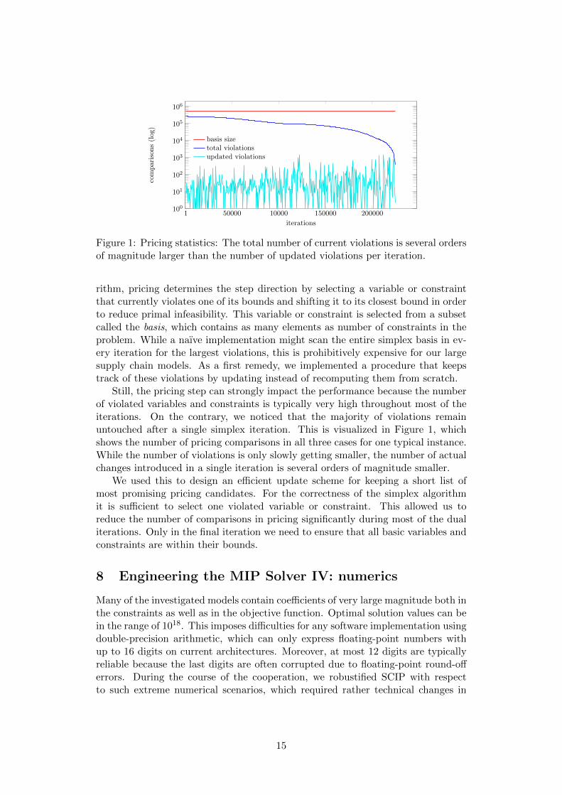
Figure 1: Pricing statistics: The total number of current violations is several ordersof magnitude larger than the number of updated violations per iteration.

rithm, pricing determines the step direction by selecting a variable or constraintthat currently violates one of its bounds and shifting it to its closest bound in orderto reduce primal infeasibility. This variable or constraint is selected from a subsetcalled the basis, which contains as many elements as number of constraints in theproblem. While a naıve implementation might scan the entire simplex basis in ev-ery iteration for the largest violations, this is prohibitively expensive for our largesupply chain models. As a first remedy, we implemented a procedure that keepstrack of these violations by updating instead of recomputing them from scratch.

Still, the pricing step can strongly impact the performance because the numberof violated variables and constraints is typically very high throughout most of theiterations. On the contrary, we noticed that the majority of violations remainuntouched after a single simplex iteration. This is visualized in Figure 1, whichshows the number of pricing comparisons in all three cases for one typical instance.While the number of violations is only slowly getting smaller, the number of actualchanges introduced in a single iteration is several orders of magnitude smaller.

We used this to design an efficient update scheme for keeping a short list ofmost promising pricing candidates. For the correctness of the simplex algorithmit is sufficient to select one violated variable or constraint. This allowed us toreduce the number of comparisons in pricing significantly during most of the dualiterations. Only in the final iteration we need to ensure that all basic variables andconstraints are within their bounds.

8 Engineering the MIP Solver IV: numerics

Many of the investigated models contain coefficients of very large magnitude both inthe constraints as well as in the objective function. Optimal solution values can bein the range of 1018. This imposes difficulties for any software implementation usingdouble-precision arithmetic, which can only express floating-point numbers withup to 16 digits on current architectures. Moreover, at most 12 digits are typicallyreliable because the last digits are often corrupted due to floating-point round-offerrors. During the course of the cooperation, we robustified SCIP with respectto such extreme numerical scenarios, which required rather technical changes in

15

details of the MIP solving process. In the following, we try to give only a fewselected examples.

Per default, SCIP treats all values above 1020 as infinity. We changed thislimit to 1030 in order to prevent cutting off very large numbers. Additionally, weintroduced a safety threshold of 1015; larger values are handled with special care,e.g., by deactivating bound tightening on constraints with such large numbers.

Furthermore, activity-based bound tightening relies heavily on so-called mini-mal and maximal activities, which represent lower and upper bounds on the con-straint function. For performance reasons, these activities are usually updatedwhenever the bound of a variable changes instead of being recomputed from scratchwhen accessed. However, these updates are prone to numerical errors, in particularif an update reduces their absolute value by several orders of magnitude. There-fore, we added a method checking the reliability of an update; if necessary, thevalue is marked as unreliable and recomputed from scratch next time it is used.This helped to avoid several cases of incorrect bound tightenings on supply chaininstances with very large coefficients.

Our last example is related to presolving. Although the preprocessing phasetransforms the model into a mathematically equivalent formulation, it may happenthat a solution to this transformed problem is not feasible after mapping it back tothe original formulation. This is due to the use of tolerances, usually in the rangeof 10−6 to 10−9, that help to cope with floating-point round-off errors.

Like most MIP solvers, SCIP uses a mixture of relative and absolute tolerancesfor checking feasibility. While relative tolerances are stable with respect to scalingof a constraint, this does not hold for absolute checks as illustrated by the followingexample:

105x− y = 0scaling−−−−→by 10−5

x− 10−5y = 0

The solution (x?, y?) = (1, 100000.05) is feasible for the scaled equation, since theconstraint is only violated by 5 ·10−7, which is below the tolerance of 10−6. On theother hand, the original equation is violated by 0.05, which is beyond the acceptedtolerance.

In order to improve the consistency of our tolerances under scaling, we addedthe option to consider the violation relative to the largest contribution of a variableto the left-hand side, i.e., solution value of the variable multiplied by its coefficientin the constraint. In the previous example, this check finds the solution (x?, y?) =(1, 100000.05) feasible also for the original constraint since the check is done relativeto 100000.05 which is the largest contribution of a variable.

In the supply chain instances discussed in this paper, this modified check isparticularly important for stock level constraints. Their right-hand side is typicallyzero while the stock levels as well as in- and out-flows can have very high values inmillions or billions. An absolute tolerance of 10−6 is impractical in those cases andcannot be achieved given the use of floating-point arithmetic.

9 Quantifying progress

In the literature, a very popular measure for comparing MIP solver performance isthe (average) running time to proven optimality. In our project, however, we apply

16

11

22

33

44

55

# Instancesoptimal solution

gap below 1%

gap below 10%

any solution no solution

Version SCIP1.2.0

SCIP2.0.0

SCIP2.1.0

SCIP3.0.0

SCIP3.1.0

Figure 2: For each SCIP version the solution quality for the instances in the test setis illustrated. The number of found solutions is continuously increasing from version toversion. The same holds for the solution quality measured by the integrality gap withinthe time limit.

a more customer-oriented measure. For each benchmark instance, there is a timelimit within which the customer expects to obtain a high-quality solution. Becauseof the challenging nature of the instances and the often tight limits, many bench-mark instances cannot be solved to optimality within the given time. Therefore,our foremost measure is the best primal bound computed within this time limit,i.e., the objective function value of the best solution found by SCIP.

Figure 2 classifies the instances in our test set according to the quality of theprimal bound at the end of the instance-specific time limit into the following cate-gories: a provably optimal solution is returned, the final optimality gap is below 1%(near-optimal), below 10% (high-quality), a feasible solution with worse optimalitygap is returned, and no solution could be found at all, which is considered a failure.

As can be seen, we managed to improve the solution quality with every newrelease of SCIP and eventually were able to compute solutions to all but one probleminstance. Note that the failing instance is an LP with more than 5 million variablesand constraints. This does not mean that the SNP Optimizer is not able to solvethis instances at all, only that the customer needs to wait for the result longer thanthe desired time limit. In our cooperation, we defined tight time limits in order toset ambitious goals.

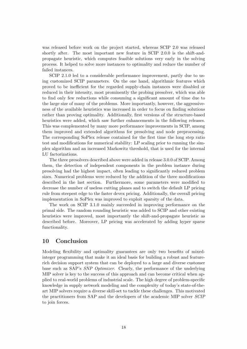
In order to also compare the speed at which improving solutions are foundwe depict the development of the mean primal gap over all instances, similar assuggested by Berthold (2013). In Figure 3, we can see a continuous improvementfrom one version to the next concerning this measure. Over the course of theproject, improving solutions were found earlier in the solving process while alsothe overall primal gap could be decreased significantly. In the following, we shortlypresent how this progress was achieved.

Both SCIP 1.2.0 and SCIP 2.0.0 were run with default settings. SCIP 1.2.0

17

was released before work on the project started, whereas SCIP 2.0 was releasedshortly after. The most important new feature in SCIP 2.0.0 is the shift-and-propagate heuristic, which computes feasible solutions very early in the solvingprocess. It helped to solve more instances to optimality and reduce the number offailed instances.

SCIP 2.1.0 led to a considerable performance improvement, partly due to us-ing customized SCIP parameters. On the one hand, algorithmic features whichproved to be inefficient for the regarded supply-chain instances were disabled orreduced in their intensity, most prominently the probing presolver, which was ableto find only few reductions while consuming a significant amount of time due tothe large size of many of the problems. More importantly, however, the aggressive-ness of the available heuristics was increased in order to focus on finding solutionsrather than proving optimality. Additionally, first versions of the structure-basedheuristics were added, which saw further enhancements in the following releases.This was complemented by many more performance improvements in SCIP, amongthem improved and extended algorithms for presolving and node preprocessing.The corresponding SoPlex release contained for the first time the long step ratiotest and modifications for numerical stability: LP scaling prior to running the sim-plex algorithm and an increased Markowitz threshold, that is used for the internalLU factorizations.

The three presolvers described above were added in release 3.0.0 of SCIP. Amongthem, the detection of independent components in the problem instance duringpresolving had the highest impact, often leading to significantly reduced problemsizes. Numerical problems were reduced by the addition of the three modificationsdescribed in the last section. Furthermore, some parameters were modified todecrease the number of useless cutting planes and to switch the default LP pricingrule from steepest edge to the faster devex pricing. Additionally, the overall pricingimplementation in SoPlex was improved to exploit sparsity of the data.

The work on SCIP 3.1.0 mainly succeeded in improving performance on theprimal side. The random rounding heuristic was added to SCIP and other existingheuristics were improved, most importantly the shift-and-propagate heuristic asdescribed before. Moreover, LP pricing was accelerated by adding hyper sparsefunctionality.

10 Conclusion

Modeling flexibility and optimality guarantees are only two benefits of mixed-integer programming that make it an ideal basis for building a robust and feature-rich decision support system that can be deployed to a large and diverse customerbase such as SAP’s SNP Optimizer. Clearly, the performance of the underlyingMIP solver is key to the success of this approach and can become critical when ap-plied to real-world problems of industrial scale. The high degree of problem-specificknowledge in supply network modeling and the complexity of today’s state-of-the-art MIP solvers require a diverse skill-set to tackle these challenges. This motivatedthe practitioners from SAP and the developers of the academic MIP solver SCIPto join forces.

18

0 20 40 60 80 1000

20

40

60

80

100

Time (percentage)

Mea

np

rim

alga

p SCIP 1.2.0SCIP 2.0.0SCIP 2.1.0SCIP 3.0.0SCIP 3.1.0

Figure 3: The comparison of the primal integrals using normalized time limits demon-strates that from version to version better solutions are found earlier during the solutionprocess.

In this article, we tried to show that the successes of our cooperation could onlybe achieved by algorithmic improvements on many different levels, both externaland internal to the MIP solver. We managed to exploit supply-chain-specific struc-tures without tying ourselves to specific models. And we learned that some featuresare even better exploited inside the general MIP solver, which may seem counter-intuitive at first. To give only one simple example, we observed that differentcomponents of the model may become disconnected only during the preprocessingphase of the solver after it has identified fixed linking variables or redundant linkingconstraints through a large collection of mathematical reduction techniques.

As a result, we achieved drastic improvements of the SCIP performance forsupply chain planning problems. We demonstrated this in particular with respectto the quality of the primal solutions obtained within ambitious time limits specifiedaccording to instance size and user requirements.

Acknowledgments. We want to thank SAP for their long-term financial andpersonal support. In addition, this work has been supported by the ResearchCampus Modal Mathematical Optimization and Data Analysis Laboratories fundedby the Federal Ministry of Education and Research (BMBF Grant 05M14ZAM).Furthermore, we acknowledge funding through the DFG SFB/Transregio 154. Allresponsibilty for the content of this publication is assumed by the authors.

References

Tobias Achterberg and Roland Wunderling. Mixed integer programming: Analyzing12 years of progress. In Michael Junger and Gerhard Reinelt, editors, Facets ofCombinatorial Optimization, pages 449–481. Springer Berlin Heidelberg, 2013. doi:10.1007/978-3-642-38189-8 18.

Timo Berthold. Measuring the impact of primal heuristics. Operations Research Letters,41(6):611 – 614, 2013. doi: 10.1016/j.orl.2013.08.007.

Timo Berthold and Gregor Hendel. Shift-and-propagate. Journal of Heuristics, 21(1):73 –106, 2014. doi: 10.1007/s10732-014-9271-0.

19

Robert Bixby and Edward Rothberg. Progress in computational mixed integerprogramming–a look back from the other side of the tipping point. Annals of Op-erations Research, 149:37–41, 2007. doi: 10.1007/s10479-006-0091-y. URL http:

//dx.doi.org/10.1007/s10479-006-0091-y.

Matteo Fischetti and Michele Monaci. Proximity search for 0-1 mixed-integer con-vex programming. Journal of Heuristics, 20(6):709–731, 2014. doi: 10.1007/s10732-014-9266-x.

John J. Forrest and Donald Goldfarb. Steepest-edge simplex algorithms for linear program-ming. Mathematical Programming, 57(1):341–374, 1992. doi: 10.1007/BF01581089.URL http://dx.doi.org/10.1007/BF01581089.

Gerald Gamrath, Timo Berthold, Stefan Heinz, and Michael Winkler. Structure-basedprimal heuristics for mixed integer programming. In Optimization in the RealWorld, volume 13, pages 37 – 53. 2015a. ISBN 978-4-431-55419-6. doi: 10.1007/978-4-431-55420-2\ 3.

Gerald Gamrath, Thorsten Koch, Alexander Martin, Matthias Miltenberger, and DieterWeninger. Progress in presolving for mixed integer programming. MathematicalProgramming Computation, 7(4):367 – 398, 2015b. doi: 10.1007/s12532-015-0083-5.

J. A. Julian Hall and Ken I. M. McKinnon. Hyper-sparsity in the revised simplex methodand how to exploit it. Comp. Opt. and Appl., 32(3):259–283, 2005. doi: 10.1007/s10589-005-4802-0. URL http://dx.doi.org/10.1007/s10589-005-4802-0.

Ellis L Johnson and Manfred W Padberg. Degree-two inequalities, clique facets, and biper-fect graphs. North-Holland Mathematics Studies, 66:169–187, 1982.

Ed Klotz. Identification, assessment, and correction of ill-conditioning and numerical in-stability in linear and integer programs. In Alexandra Newman and Janny Leung,editors, Bridging Data and Decisions, TutORials in Operations Research, pages 54–108. 2014. doi: 10.1287/educ.2014.0130.

Thorsten Koch, Tobias Achterberg, Erling Andersen, Oliver Bastert, Timo Berthold,Robert E. Bixby, Emilie Danna, Gerald Gamrath, Ambros M. Gleixner, Stefan Heinz,Andrea Lodi, Hans Mittelmann, Ted Ralphs, Domenico Salvagnin, Daniel E. Steffy,and Kati Wolter. MIPLIB 2010. Mathematical Programming Computation, 3(2):103–163, 2011. doi: 10.1007/s12532-011-0025-9. URL http://mpc.zib.de/index.php/

MPC/article/view/56/28.

Ekaterina Kostina. The long step rule in the bounded-variable dual simplex method:Numerical experiments. Mathematical Methods of Operations Research, 55(3):413–429, 2002. doi: 10.1007/s001860200188. URL http://dx.doi.org/10.1007/

s001860200188.

Hugues Marchand and Laurence A. Wolsey. Aggregation and mixed integer rounding tosolve MIPs. Operations Research, 49(3):363–371, 2001. doi: 10.1287/opre.49.3.363.11211.

Martin W. P. Savelsbergh. Preprocessing and probing techniques for mixed integer pro-gramming problems. ORSA Journal on Computing, 6:445–454, 1994.

Hartmut Stadtler, Bernhard Fleischmann, Martin Grunow, Herbert Meyr, and ChristopherSurie. Advanced Planning in Supply Chains. Management for Professionals. Springer-Verlag Berlin Heidelberg, 2012. doi: 10.1007/978-3-642-24215-1.

Chris Wallace. ZI round, a MIP rounding heuristic. Journal of Heuristics, 16(5):715–722, 2010. doi: 10.1007/s10732-009-9114-6. URL http://dx.doi.org/10.1007/

s10732-009-9114-6.

Roland Wunderling. Paralleler und objektorientierter Simplex-Algorithmus. PhD thesis,Technische Universitat Berlin, 1996.

20

Appendix: Mathematical Details

This appendix presents details about the mathematical model used in SNP Opti-mization and about our benchmarking methodology.

Mixed-integer linear programming models

To give a better insight on the structure and the connection between business andmathematical programming a basic supply chain model is elaborated here. Everylinear programming model consists of the two fundamental parts: the objectivefunction, subject of minimization or maximization, and the constraint matrix, con-sisting of different inequalities and restricting the solution space. In the case ofcost based supply chain models, all arising costs—like transport costs, productioncosts, and most importantly non-delivery costs—constitute the objective function,which then needs to be minimized. Costs usually are connected to variables thatneed to be calculated by the solver. These are exactly the variables the customer isinterested in: how many products need to be transported on which transportationlane or how many products need to be produced in this special factory.

The supply chain structure itself yields numerous constraints. These emergefrom restrictions entered by the customer like limited resource capacities but alsofrom essential requirements like stock balance consistency. Step by step we con-struct all relevant constraints needed to formulate the stock balance equation onthe one hand and an opposed type of constraint resulting form the capacity resourcerestriction on the other. Keep in mind that this is only a rather simple exemplarymodel, without any claims of completeness.

Definition of sets

T set of time bucketsL set of locationsD set of demandsDt set of demands in time bucket tDl set of demands at location lA set of arcsAl set of arcs with location l as destinationAl set of arcs with location l as originP set of productsPLl set of products that are handled at location lPAa set of products that can be transported on arc aOl set of production Models at location lR set of resources

Demands

The main goal of supply chain management is to satisfy requested demands. How-ever, there are no cost-relevant benefits or rewards created by satisfying a demand.Instead, in order to initiate activity within the supply chain despite the costs of

21

production and transportation, the model incorporates artificial non-delivery penal-ties.

Definition of parameters:dt demand d in bucket tDQdt quantity of demand d in bucket tδdt maximum allowed lateness for demand d in bucket tCNdt non-delivery costs for demand d in bucket tCLdt(t

′) late delivery costs delivering (t′ − t) buckets late

Definition of variables:V Ndt quantity not delivered for demand d in bucket tV Ldt(t

′) quantity delivered in bucket t′ for demand d in bucket t

A demand may allow a late delivery by some time buckets. To obtain the non-delivered amount regarding one demand in a bucket all deliveries for that demand,even the delayed ones, are subtracted from the original demand quantity in thatbucket:

V Ndt = DQdt −t+δt∑t′=t

V Ldt(t′)

In addition to the constraints there are costs that need to be respected. All costequations will be displayed for one single time bucket only. To obtain total costsall relevant time buckets need to be summed up. Non-delivery costs are calculatedby: ∑

dt∈Dt

CNdt · V Ndt

Where late delivery is allowed, additional costs need to be incurred to motivateon-time delivery. These late delivery costs are calculated by:

∑dt∈Dt

t+δdt∑t′=t+1

CLdt(t′) · V Ldt(t′)

Transport

To make transfer of products possible, transport lines between locations, here calledarcs, need to be modeled.

Definition of parameters:CTap(t) cost of transporting one unit of product p via arc a in bucket t

Definition of variables:V Tap(t) quantity of product p transported on arc a in bucket t

For simplicity, we will not consider any restrictions on these arcs. But theremay still arise transport costs when shipping products form one location to another:∑

a∈A

∑p∈PAa

CTap(t) · V Tap(t)

22

Production

Another basic activity of the supply chain is the production of a product by con-suming other products. This is modeled by production models, containing allinformation on input and output products.

Definition of parameters:COo(t) cost of applying production model o ∈ Ol once at location l in bucket t

Definition of variables:V Oo(t) continuous number of applications of production model o ∈ Ol at location l in bucket t

Similarly to transports, we will neither consider limitations nor possible coeffi-cients for input or output. Production costs are computed by:∑

l∈L

∑o∈Ol

COo(t) · V Oo(t)

Procurement

Procurement models external acquisitions of products and makes them available atspecific locations.

Definition of variables:CPlp(t) cost of procuring product p at location l in bucket t

Definition of variables:V Plp(t) quantity procured of product p at location l in bucket t

Procurement costs may be incurred, especially when weighting external sourcingagainst internal production. The costs are calculated by:∑

l∈L

∑p∈PLl

CPlp(t) · V Plp(t)

Stock level

Products stored at locations and existing stock from previous time buckets need tobe accounted. But there can be further restrictions, for instance on stock quantity.

Definition of parameters:PR+

op(t) output quantity of product p from production model o in bucket t

PR−op(t) input quantity of product p to production model o in bucket t

Definition of variables:V Slp(t) stock level at location l of product p in bucket tCSlp(t) cost of storing product p at location l in bucket t

For products kept in stock at a location so called inventory holding costs canbe incurred:

23

∑l∈L

∑p∈PLl

CSlp(t) · V Slp(t)

We finally have introduced all relevant variables and equations to define stockbalance equations, which contain all information on input and output to and froma location by production, transport or procurement, as well as on stock quantitiesfrom the previous time bucket:

V Slp(t) = V Slp(t− 1) + V Plp(t) +∑o∈Ol

PR+op(t) · V Oo(t) +

∑a∈Al

V Tap(t)

−∑o∈Ol

PR−op(t) · V Oo(t)−∑a∈Al

V Tap(t)−∑dτ∈Dl

V Ldτp(t)

Resource capacities

Resource restrictions can be considered in different activities. For simplicity, werefer only to production as a showcase. Resource capacities in production usuallyrepresent allocatable time on production machines or available man hours. There-fore different product lines may share the same resources.

Definition of parameters:RRor(t) requirement of resource r for production model o in bucket tRCr(t) capacity of resource r in bucket t

There are no costs for resource consumption. Production resource capacityrestrictions are mapped to the constraints:∑

o∈Ol

RRor(t) · V Oo(t) ≤ RCr(t)

Production with minimum lot sizes

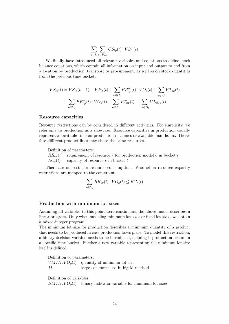
Assuming all variables to this point were continuous, the above model describes alinear program. Only when modeling minimum lot sizes or fixed lot sizes, we obtaina mixed-integer program.The minimum lot size for production describes a minimum quantity of a productthat needs to be produced in case production takes place. To model this restriction,a binary decision variable needs to be introduced, defining if production occurs ina specific time bucket. Further a new variable representing the minimum lot sizeitself is defined.

Definition of parameters:VMIN V Oo(t) quantity of minimum lot sizeM large constant used in big-M method

Definition of variables:BMIN V Oo(t) binary indicator variable for minimum lot sizes

24

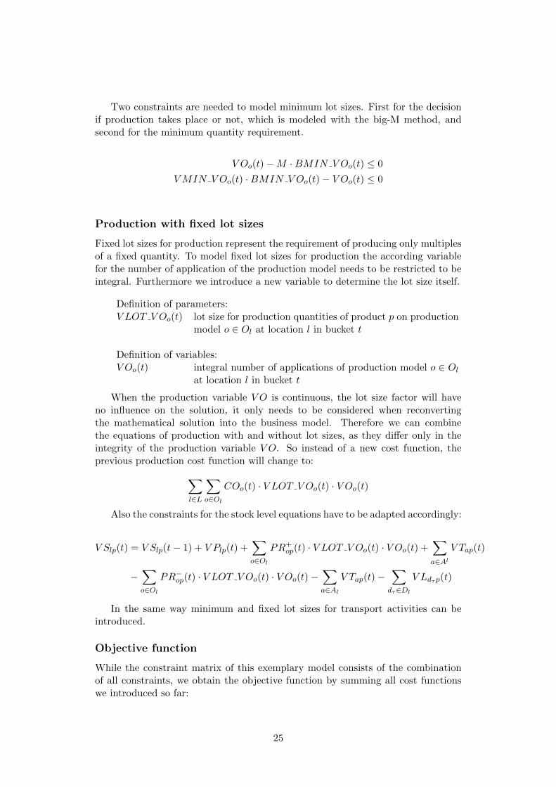
Two constraints are needed to model minimum lot sizes. First for the decisionif production takes place or not, which is modeled with the big-M method, andsecond for the minimum quantity requirement.

V Oo(t)−M ·BMIN V Oo(t) ≤ 0

VMIN V Oo(t) ·BMIN V Oo(t)− V Oo(t) ≤ 0

Production with fixed lot sizes

Fixed lot sizes for production represent the requirement of producing only multiplesof a fixed quantity. To model fixed lot sizes for production the according variablefor the number of application of the production model needs to be restricted to beintegral. Furthermore we introduce a new variable to determine the lot size itself.

Definition of parameters:V LOT V Oo(t) lot size for production quantities of product p on production

model o ∈ Ol at location l in bucket t

Definition of variables:V Oo(t) integral number of applications of production model o ∈ Ol

at location l in bucket t

When the production variable V O is continuous, the lot size factor will haveno influence on the solution, it only needs to be considered when reconvertingthe mathematical solution into the business model. Therefore we can combinethe equations of production with and without lot sizes, as they differ only in theintegrity of the production variable V O. So instead of a new cost function, theprevious production cost function will change to:∑

l∈L

∑o∈Ol

COo(t) · V LOT V Oo(t) · V Oo(t)

Also the constraints for the stock level equations have to be adapted accordingly:

V Slp(t) = V Slp(t− 1) + V Plp(t) +∑o∈Ol

PR+op(t) · V LOT V Oo(t) · V Oo(t) +

∑a∈Al

V Tap(t)

−∑o∈Ol

PR−op(t) · V LOT V Oo(t) · V Oo(t)−∑a∈Al

V Tap(t)−∑dτ∈Dl

V Ldτp(t)

In the same way minimum and fixed lot sizes for transport activities can beintroduced.

Objective function

While the constraint matrix of this exemplary model consists of the combinationof all constraints, we obtain the objective function by summing all cost functionswe introduced so far:

25

ObjFunct =∑dτ∈D

τ+δdτ∑t′>τ

CLdτ (t′) · V Ldτ (t′) + CNdτ · V Ndτ

+∑t∈T

∑a∈A

∑p∈PAa

CTap(t) · V Tap(t)

+∑l∈L

∑o∈Ol

COo(t) · V LOT V Oo(t) · V Oo(t)

+∑l∈L

∑p∈PLl

(CPlp(t) · V Plp(t) + CSlp(t) · V Slp(t)

)This objective function will then be subject of minimization.

Further features

The variables and constraints described above comprise the basic core of the math-ematical model. In addition, the SNP Optimization supports further features thatcannot be discussed here in detail due to lack of space, for instance:

• safety stock: try to keep material inventory at a certain minimum level

• shelf life: limit material inventory not to exceed a certain maximum level

• extension capacity: extend resource capacity at some costs

• cost functions: convex and concave piecewise linear cost functions on basicdecisions such as production, transport, or inventory

• substitution: satisfy product demands by substitute products

• quota arrangements: try to keep quota arrangements between alternative sourcesof supply

• subcontracting: consider external suppliers of certain products

• fix material flows: some production may incur fix material flows independentof the number of produced lots

• fix resource consumption: some production may incur fix resource capacityconsumption, independent of the number of produced lots

Benchmarking methodology

All computations were performed on Intel Xeon X5672 CPUs with 3.2 GHz and64 GB of main memory, running only one problem instance at a time in order tomeasure solution times accurately.

The used test set consists of a representative subset of all training instancessupplied by SAP within our cooperation. They model diverse real-world supply

26

chain scenarios, each in multiple levels of detail, leading to a variety of problemsizes. The given time limits vary between 30 and 7200 seconds, depending mostlyon the problem size. Some instances are pure LPs, i.e., there are no integer orbinary variables, whereas the majority of instances are either mixed-integer ormixed-binary problems. The amount of integrality is usually below 10% of thevariables but can be as high as 30% for one problem class.

While pure LPs need to be solved to optimality, MIPs have a so-called optimalitygap, signifying how far the solution value of an integer feasible solution is away fromthat of the optimal one. Whenever a new incumbent, i.e., an improved solution isfound, the optimality gap is reduced and this development can be represented asa monotonously decreasing function. To measure how quickly the quality of thebest known primal solutions approaches the optimum, one can employ the primalintegral (Berthold 2013).

For practical applications, this measure is richer than the traditional way ofcomparing solution times or solution qualities at the limit limit, especially in thedescribed setting of this project, where our main goal is to provide good solutionsquickly. To obtain the version-to-version progress displayed in Figure 3, we averagedover the primal integrals for all instances in the test set. In order to account foreach instance equally, the primal bound function was normalized by the instance-dependent time limits.

27