Tackling Large State Spacesin Performance Modelling?

William J. Knottenbelt Jeremy T. Bradley{wjk,jb}@doc.ic.ac.uk

Department of Computing, Imperial College London, Huxley Building,South Kensington, London SW7 2AZ, UK

Abstract. Stochastic performance models provide a powerful way ofcapturing and analysing the behaviour of complex concurrent systems.Traditionally, performance measures for these models are derived by gen-erating and then analysing a (semi-)Markov chain corresponding to themodel’s behaviour at the state-transition level. However, and especiallywhen analysing industrial-scale systems, workstation memory and com-pute power is often overwhelmed by the sheer number of states.This chapter explores an array of techniques for analysing stochasticperformance models with large state spaces. We concentrate on explicittechniques suitable for unstructured state spaces and show how memoryand run time requirements can be reduced using a combination of prob-abilistic algorithms, disk-based solution techniques and communication-efficient parallelism based on hypergraph-partitioning. We apply thesemethods to different kinds of performance analysis, including steady-state and passage-time analysis, and demonstrate them on case studyexamples.

1 Introduction and Context

Modern computer and communication systems are increasingly complex. Whereasin the past systems were usually controlled by a single program running on asingle machine with a single flow of control, recent years have seen the rise oftechnologies such as multi-threading, parallel and distributed computing and ad-vanced communication networks. The result is that modern systems are complexwebs of cooperating subsystems with many possible interactions.

In the face of this complexity, it is an extremely challenging task for system de-signers to guarantee satisfactory system operation in terms of both correctnessand performance. Unfortunately, attempts to predict dynamic behaviour usingintuition or “rules of thumb” are doomed to failure because designers cannot fore-see the many millions of possible interactions between components. Likewise, ad? Based on work carried out in collaboration with Nicholas J. Dingle, Peter G. Harrison

and Aleksandar Trifunovic

hoc testing cannot expose a sufficient number of execution paths. Consequentlythe likelihood of problems caused by subtle bugs such as race conditions is high.

One way to meet the above challenge using a rigorous engineering approachis to use formal modelling techniques to mechanically verify correctness andperformance properties. The advantage of this style of approach over ad hocmethods has been clearly demonstrated in recent work on the formal modelchecking of file system code – in [1] the authors use a breadth-first state spaceexploration of all possible execution paths and failure points to automaticallyuncover several (serious and hitherto undiscovered) errors in ten widely-used filesystems.

Formal techniques which consider all possible system behaviours can likewisebe brought to bear on the problem which is the primary concern of the presentchapter, namely that of predicting system performance. Our specific focus ison analytical performance modelling techniques which make use of Markov andsemi-Markov chains to model the low-level stochastic behaviour of a system.(Semi-)Markov chains are limited to describing systems that have discrete statesand which satisfy the property that the future behaviour of the system dependsonly on the current state. Despite these limitations, they are flexible enough tomodel many phenomena found in complex concurrent systems such as blocking,synchronisation, preemption, state-dependent routing and complex traffic arrivalprocesses. In addition, tedious manual enumeration of all possible system states isnot necessary. Instead, chains can be automatically derived from several widely-used high level modelling formalisms such as Stochastic Petri Nets and StochasticProcess Algebras.

A major difficulty often encountered with this approach is the state space explo-sion problem whereby workstation memory and compute power are overwhelmedby the sheer number of states that emerge from complex models. Consequently,a major challenge and focus of research is the development of methods and datastructures which minimise the memory and runtime required to generate andsolve very large (semi-)Markov chains. One approach to this “largeness” prob-lem is to restrict the structure of models that can be analysed. This allows for theapplication of efficient techniques which exploit the restricted structure. Sincethese techniques are covered in other chapters, we do not discuss them furtherhere, preferring unrestricted scalable parallel and distributed algorithms whichare able to efficiently leverage the compute power, memory and disk space ofseveral processors.

2 Stochastic Processes

At the lowest level, the performance modelling of a system can be accomplishedby identifying all possible configurations, or states, that the system can enter anddescribing the ways in which the system can move between those states. This

is termed the state-transition level behaviour of the model, and the changes instate as time progresses describe a stochastic process. We focus on those stochas-tic processes which belong to the class known as Markov processes, specificallycontinuous-time Markov chains (CTMCs) and the more general semi-Markovprocesses (SMPs).

Consider a random variable χ which takes on different values at different timest. The sequence of random variables χ(t) is said to be a stochastic process. Thedifferent values which χ(t) can take, describe the state space of the stochasticprocess.

A stochastic process can be classified by the nature of its state space and of itstime parameter. If the values in the state space of χ(t) are finite or countablyinfinite, then the stochastic process is said to have a discrete state space (andmay also be referred to as a chain). Otherwise, the state space is said to becontinuous. Similarly, if the times at which χ(t) is observed are also countable,the process is said to be a discrete-time process. Otherwise, the process is said tobe a continuous-time process. In this chapter, all stochastic processes consideredhave discrete and finite state spaces, and we focus mainly on those which evolvein continuous time.

Definition 1. A Markov process is a stochastic process in which the Markovproperty holds. Given that χ(t) = xt indicates that the state of the process χ(t)at time t is xt, this property stipulates that:

IP(χ(t) = x | χ(tn) = xn, χ(tn−1) = xn−1, . . . , χ(t0) = x0

)

= IP(χ(t) = x | χ(tn) = xn

)

for t > tn > tn−1 > . . . > t0

That is, the future evolution of the system depends only on the current state andnot on any prior states.

Definition 2. A Markov process is said to be homogeneous if it is invariant toshifts in time:

IP(χ(t + s) = x | χ(tn + s) = xn

)= IP

(χ(t) = x | χ(tn) = xn

)

2.1 Continuous-time Markov Chains

There exists a family of Markov processes with discrete state spaces but whosetransitions can occur at arbitrary points in time; we call these continuous-timeMarkov chains (CTMCs). An homogeneous N -state CTMC has state at timet denoted χ(t). Its evolution is described by an N × N generator matrix Q,where qij is the infinitesimal rate of moving from state i to state j (i 6= j), andqii = −∑

j 6=i qij .

The Markov property imposes a memoryless restriction on the distribution of thesojourn times of states in a CTMC. The future evolution of the system thereforedoes not depend on the evolution of the system up until the current state, nordoes it depend on how long the system has already been in the current state.This means that the sojourn time ν in any state must satisfy:

IP(ν ≥ s + t | ν ≥ t) = IP(ν ≥ s) (1)

A consequence of Eq. (1) is that all sojourn times in a CTMC must be exponen-tially distributed (see [2] for a proof that this is the only continuous distributionfunction which satisfies this condition). The rate out of state i, and thereforethe parameter of the sojourn time distribution, is µi and is equal to the sum ofall rates out of state i, that is µi = −qii. This means that the density functionof the sojourn time in state i is fi(t) = µi e−µit and the average sojourn time instate i is µ−1

i .

A concept that is fundamental to reasoning about the performance of a CTMCis that of its steady state distribution – that is the long-run average proportionof time that a system spends in each of its states.

Definition 3. A Markov chain is said to be irreducible if every state commu-nicates with every other state, i.e. if for every pair of states i and j there is apath from state i to j and vice versa.

Definition 4. The steady-state probability distribution {πj} of an irreducible,homogeneous CTMC is given by:

πj = limt→∞

IP(χ(t) = j | χ(0) = i)

For a finite, irreducible and homogeneous CTMC, the steady-state probabilities{πj} always exist and are independent of the initial state distribution. They areuniquely given by the solution of the equations:

−qjjπj +∑

k 6=j

qkjπk = 0 subject to∑

i

πi = 1

Again, this can be expressed in matrix vector form (in terms of the vector πwith elements {π1, π2, . . . , πN} and the matrix Q defined above) as:

πQ = 0 (2)

A CTMC also has an embedded discrete-time Markov chain (EMC) which de-scribes the behaviour of the chain at state-transition instants, that is to say theprobability that the next state is j given that the current state is i. The EMCof a CTMC has a one-step N ×N transition matrix P where pij = −qij/qii fori 6= j and pij = 0 for i = j.

The steady-state distribution enables us to compute various basic resource-basedmeasures (such as utilisation, mean throughput, and so on); however, more ad-vanced response-time measures (such as quantiles of response time) require afirst passage time analysis.

Definition 5. Consider a finite, irreducible CTMC with N states {1, 2, . . . , N}and generator matrix Q. If χ(t) denotes the states of the CTMC at time t (t ≥ 0)and N(t) denotes the number of state transitions which have occurred by timet, the first passage time from a single source marking i into a non-empty set oftarget markings j is:

Pij(t) = inf{u > 0 : χ(t + u) ∈ j, N(t + u) > N(t), χ(t) = i}

When the CTMC is stationary and time-homogeneous this quantity is indepen-dent of t:

Pij = inf{u > 0 : χ(u) ∈ j, N(u) > 0, χ(0) = i} (3)

That is, the first time the system enters a state in the set of target states j, giventhat the system began in the source state i and at least one state transition hasoccurred. Pij is a random variable with probability density function fij(t) suchthat:

IP(t1 < Pij < t2) =∫ t2

t1

fij(t) dt for 0 ≤ t1 < t2

In order to determine fij(t) it is necessary to convolve the state holding-timedensity functions over all possible paths (including cycles) from state i to all ofthe states in j.

The calculation of the convolution of two functions in t-space can be more easilyaccomplished by multiplying their Laplace transforms together in s-space andinverting the result. The calculation of fij(t) is therefore achieved by calculatingthe Laplace transform of the convolution of the state holding times over allpaths between i and j and then numerically inverting this Laplace transform(see Sect. 4.3 for a description of two inversion algorithms).

In a CTMC all state sojourn times are exponentially distributed, so the densityfunction of the sojourn time in state i is µie

−µit, where µi = −qii (as before).The Laplace transform of an exponential density function with rate parameterλ is:

L{λe−λt} =λ

λ + s

Denoting the Laplace transform of the density function fij(t) of the passagetime random variable Pij as Lij(s), we proceed by means of a first-step analysis.That is, to calculate the first passage time from state i into the set of targetstates j, we consider moving from state i to its set of direct successor states kand thence from states in k to states in j. This can be expressed as the following

system of linear equations:

Lij(s) =∑

k/∈j

pik

( −qii

s− qii

)Lkj(s) +

∑

k∈j

pik

( −qii

s− qii

)(4)

The first term (i.e. the summation over non-target states k /∈ j) convolves thesojourn time density in state i with the density of the time taken for the systemto evolve from state k into a target state in j, weighted by the probability thatthe system transits from state i to state k. The second term (i.e. the summationover target states k ∈ j) simply reflects the sojourn time density in state iweighted by the probability that a transition from state i into a target state koccurs.

Given that pij = −qij/qii in the context of a CTMC, Eq. (4) can be rewrittenmore simply as:

Lij(s) =∑

k/∈j

qik

s− qiiLkj(s) +

∑

k∈j

qik

s− qii(5)

This set of linear equations can be expressed in matrix–vector form. For example,when j = {1} we have:

s− q11 −q12 · · · −q1n

0 s− q22 · · · −q2n

0 −q32 · · · −q3n

0...

. . ....

0 −qn2 · · · s− qnn

L1j(s)L2j(s)L3j(s)

...Lnj(s)

=

0q21

q31

...qn1

(6)

Our formulation of the passage time quantity in Eq. (3) states that we mustobserve at least one state-transition during the passage. In the case where i ∈ j(as for L1j(s) in the above example), we therefore calculate the density of thecycle time to return to state i rather than requiring Lij(s) = 1.

Given a particular (complex-valued) s, Eq. (5) can be solved for Lij(s) by stan-dard iterative numerical techniques for the solution of systems of linear equationsin Ax = b form. Many numerical Laplace transform inversion algorithms (suchas the Euler and Laguerre methods) can identify in advance the s-values at whichLij(s) must be calculated in order to perform the numerical inversion. There-fore, if the algorithm requires m different values of Lij(s), Eq. (5) will need tobe solved m times.

The corresponding cumulative distribution function Fij(t) of the passage timeis obtained by integrating under the density function. This integration can beachieved in terms of the Laplace transform of the density function by dividingit by s, i.e. F ∗ij(s) = Lij(s)/s. In practice, if Eq. (5) is solved as part of theinversion process for calculating fij(t), the m values of Lij(s) can be retained.Once the numerical inversion algorithm has used them to compute fij(t), these

values can be recovered, divided by s and then taken as input by the numericalinversion algorithm again to compute Fij(t). Thus, in calculating fij(t), we getFij(t) for little further computational effort.

When there are multiple source markings, denoted by the vector i, the Laplacetransform of the response time density at equilibrium is:

Li j(s) =∑

k∈i

αkLkj(s)

where the weight αk is the equilibrium probability that the state is k ∈ i at thestarting instant of the passage. This instant is the moment of entry into statek; thus αk is proportional to the equilibrium probability of the state k in theunderlying embedded (discrete-time) Markov chain (EMC) of the CTMC withone-step transition matrix P as defined in Sect. 2.1. That is:

αk ={

πk/∑

j∈i πj if k ∈ i

0 otherwise(7)

where the vector π is any non-zero solution to π = πP. The row vector withcomponents αk is denoted by α.

Uniformisation Passage time densities and quantiles in CTMCs may also becomputed through the use of uniformisation (also known as randomisation) [3–8]. This transforms a CTMC into one in which all states have the same meanholding time 1/q, by allowing “invisible” transitions from a state to itself. Thisis equivalent to a discrete-time Markov chain, after normalisation of the rows,together with an associated Poisson process of rate q.

Definition 6. The one-step transition probability matrix P which characterisesthe one-step behaviour of a uniformised DTMC is derived from the generatormatrix Q of the CTMC as:

P = Q/q + I (8)

where the rate q > maxi |qii| ensures that the DTMC is aperiodic by guaranteeingthat there is at least one single-step transition from a state to itself.

We ensure that only the first passage time density is calculated and that we donot consider the case of successive visits to a target state by making the targetstates in P absorbing. We denote by P′ the one-step transition probability matrixof the modified, uniformised chain.

The calculation of the first passage time density between two states then hastwo main components. The first considers the time to complete n hops (n =1, 2, 3, . . .). Recall that in the uniformised chain all transitions occur with rate q.The density of the time taken to move between two states is found by convolving

the state holding-time densities along all possible paths between the states. Ina standard CTMC, convolving holding times in this manner is non-trivial as,although they are all exponentially distributed, their rate parameters are differ-ent. In a CTMC which has undergone uniformisation, however, all states haveexponentially-distributed state holding-times with the same parameter q. Thismeans that the convolution of n of these holding-time densities is an n-stageErlang density with rate parameter q.

Secondly, it is necessary to calculate the probability that the transition betweena source and target state occurs in exactly n hops of the uniformised chain,for every value of n between 1 and a maximum value m. The value of m isdetermined when the value of the nth Erlang density function (the left-handterm in Eq. (9)) drops below some threshold value. After this point, furtherterms are deemed to add nothing significant to the passage time density and soare disregarded.

The density of the time to pass between a source state i and a target state j ina uniformised Markov chain can therefore be expressed as the sum of m n-stageErlang densities, weighted with the probability that the chain moves from statei to state j in exactly n hops (1 ≤ n ≤ m). This can be generalised to allowfor multiple target states in a straightforward manner; when there are multiplesource states it is necessary to provide a probability distribution across this setof states (such as the renormalised steady-state distribution calculated below inEq. (11)).

The response time between the non-empty set of source states i and the non-empty set of target states j in the uniformised chain therefore has probabilitydensity function:

fij(t) =∞∑

n=1

qntn−1e−qt

(n− 1)!

∑

k∈j

π(n)k

'm∑

n=1

qntn−1e−qt

(n− 1)!

∑

k∈j

π(n)k

(9)

where:π(n+1) = π(n)P′ for n ≥ 0 (10)

with:

π(0)k =

{0 for k /∈ iπk/

∑j∈i πj for k ∈ i

(11)

The πk values are the steady state probabilities of the corresponding state k inthe CTMC’s embedded Markov chain. When the convergence criterion:

‖π(n) − π(n−1)‖∞‖π(n)‖∞

< ε (12)

is met, for given tolerance ε, the vector π(n) is considered to have converged andno further multiplications with P′ are performed. Here, ‖x‖∞ is the infinity-normgiven by ‖x‖∞ = maxi |xi|.The corresponding cumulative distribution function for the passage time, Fij(t),can be calculated by substituting the cumulative distribution function for theErlang distribution into Eq. (9) in place of the Erlang density function term,viz.:

Fij(t) =∞∑

n=1

(1− e−qt

n−1∑

k=0

(qt)k

k!

) ∑

k∈j

π(n)k

'm∑

n=1

(1− e−qt

n−1∑

k=0

(qt)k

k!

) ∑

k∈j

π(n)k

where π(n) is defined as in Eqs. (10) and (11).

2.2 Semi-Markov Processes

Semi-Markov Processes (SMPs) are an extension of Markov processes whichallow for generally distributed sojourn times. Although the memoryless propertyno longer holds for state sojourn times, at transition instants SMPs still behavein the same way as Markov processes (that is to say, the choice of the nextstate is based only on the current state) and so share some of their analyticaltractability.

Definition 7. Consider a Markov renewal process {(χn, Tn) : n ≥ 0} where Tn

is the time of the nth transition (T0 = 0) and χn ∈ S is the state at the nthtransition. Let the kernel of this process be:

R(n, i, j, t) = IP(χn+1 = j, Tn+1 − Tn ≤ t | χn = i)

for i, j ∈ S. The continuous time semi-Markov process, {Z(t), t ≥ 0}, defined bythe kernel R, is related to the Markov renewal process by:

Z(t) = χN(t)

where N(t) = max{n : Tn ≤ t}, i.e. the number of state transitions that havetaken place by time t. Thus Z(t) represents the state of the system at time t.

We consider only time-homogeneous SMPs in which R(n, i, j, t) is independentof n, that is for:

R(i, j, t) = IP(χn+1 = j, Tn+1 − Tn ≤ t | χn = i) for any n ≥ 0= pijHij(t)

where pij = IP(χn+1 = j | χn = i) is the state transition probability betweenstates i and j and Hij(t) = IP(Tn+1 − Tn ≤ t | χn+1 = j, χn = i), is the sojourntime distribution in state i when the next state is j. An SMP can therefore becharacterised by two matrices P and H with elements pij and Hij respectively.

Semi-Markov processes can be analysed for steady-state performance metricsin a similar manner as DTMCs and CTMCs. To do this, we need to know thesteady-state probabilities of the SMP’s embedded Markov chain and the averagetime spent in each state. The first of these can be calculated by solving π = πP,as in the case of DTMCs. The average time in state i, IE[τi], is the weighted sumof the averages of the sojourn time in the state i when going to state j, IE[τij ],for all successor states j of i, that is:

IE[τi] =∑

j

pijIE[τij ]

The steady-state probability of being in state i of the SMP is then:

φi =πiIE[τi]∑N

m=1 πmIE[τm](13)

That is, the long-run probability of finding the SMP in state i is the probabilityof its EMC being in state i multiplied by the average amount of time the SMPspends in state i, normalised over the mean total time spent in all of the statesof the SMP.

Passage-time analysis for SMPs is also possible by extending the Laplace trans-form method for CTMCs to cater for generally-distributed state sojourn times.

Definition 8. Consider a finite, irreducible, continuous-time semi-Markov pro-cess with N states {1, 2, . . . , N}. Recalling that Z(t) denotes the state of the SMPat time t (t ≥ 0), the first passage time from a source state i at time t into anon-empty set of target states j is:

Pij(t) = inf{u > 0 : Z(t + u) ∈ j, N(t + u) > N(t) | Z(t) = i} (14)

For a stationary time-homogeneous SMP, Pij(t) is independent of t and we have:

Pij = inf{u > 0 : Z(u) ∈ j, N(u) > 0 | Z(0) = i} (15)

Pij has an associated probability density function fij(t) such that the passagetime quantile is given as:

IP(t1 < Pij < t2) =∫ t2

t1

fij(t) dt for 0 ≤ t1 < t2 (16)

In general, the Laplace transform of fij , Lij(s), can be computed by solving aset of N linear equations:

Lij(s) =∑

k/∈j

r∗ik(s)Lkj(s) +∑

k∈j

r∗ik(s) for 1 ≤ i ≤ N (17)

where r∗ik(s) is the Laplace-Stieltjes transform (LST) of R(i, k, t) and is definedby:

r∗ik(s) =∫ ∞

0

e−st dR(i, k, t) (18)

Eq. (17) has a matrix–vector form where the elements of the matrix are arbitrarycomplex functions; care needs to be taken when storing such functions for even-tual numerical inversion (see Sect. 4.3). For example, when j = {1}, Eq. (17)yields:

1 −r∗12(s) · · · −r∗1N (s)0 1− r∗22(s) · · · −r∗2N (s)0 −r∗32(s) · · · −r∗3N (s)...

.... . .

...0 −r∗N2(s) · · · 1− r∗NN (s)

L1j(s)L2j(s)L3j(s)

...LNj(s)

=

r∗11(s)r∗21(s)r∗31(s)

...r∗N1(s)

(19)

When there are multiple source states, denoted by the vector i, the Laplacetransform of the passage time density at steady-state is:

Li j(s) =∑

k∈i

αkLkj(s) (20)

where the weight αk is the probability at equilibrium that the system is in statek ∈ i at the starting instant of the passage. As with CTMCs α is defined interms of π, the steady-state vector of the embedded discrete-time Markov chainwith one-step transition probability matrix P:

αk ={

πk/∑

j∈i πj if k ∈ i

0 otherwise(21)

3 Modelling Formalisms

Stochastic models are specified using graphical or symbolic languages knownas modelling formalisms. Below we describe two popular formalisms: StochasticPetri nets and Stochastic Process Algebras.

3.1 Stochastic Petri Nets

We briefly outline two types of stochastic Petri net: Generalised Stochastic PetriNets (GSPNs) which allow timed exponential and immediate transitions, andSemi-Markov Stochastic Petri Nets (SM-SPNs) which specify models with gen-erally distributed transitions.

Generalised Stochastic Petri Nets Generalised Stochastic Petri nets are anextension of Place-Transition nets, which are ordinary, untimed Petri nets. APlace-Transition net does not have firing delays associated with its transitionsand is formally defined in [2]:

Definition 9. A Place-Transition net is a 5-tuple PN = (P, T, I−, I+,M0) where

– P = {p1, . . . , pn} is a finite and non-empty set of places.– T = {t1, . . . , tm} is a finite and non-empty set of transitions.– P ∩ T = ∅.– I−, I+ : P × T → IN0 are the backward and forward incidence functions,

respectively. If I−(p, t) > 0, an arc leads from place p to transition t, and ifI+(p, t) > 0 then an arc leads from transition t to place p.

– M0 : P → IN0 is the initial marking defining the initial number of tokens onevery place.

A marking is a vector of integers representing the number of tokens on eachplace in a Petri net. The set of all markings that are reachable from the initialmarking M0 is known as the state space or reachability set of the Petri net, andis denoted by R(M0). The connections between markings in the reachability setform the reachability graph. Formally, if the firing of a transition that is enabledin marking Mi results in marking Mj , then the reachability graph contains adirected arc from marking Mi to marking Mj .

GSPNs [9] are timed extensions of Place-Transition nets with two types of tran-sitions: immediate transitions and timed transitions. Once enabled, immediatetransitions fire in zero time, while timed transitions fire after an exponentiallydistributed firing delay. Firing of immediate transitions has priority over thefiring of timed transitions.

The formal definition of a GSPN is as follows [2]:

Definition 10. A GSPN is a 4-tuple GSPN = (PN, T1, T2,W ) where

– PN = (P, T, I−, I+, M0) is the underlying Place-Transition net.– T1 ⊆ T is the set of timed transitions, T1 6= ∅,– T2 ⊂ T denotes the set of immediate transitions, T1 ∩ T2 = ∅, T = T1 ∪ T2

– W = (w1, . . . , w|T |) is an array whose entry wi is either• a (possibly marking dependent) rate ∈ IR+ of an exponential distribution

specifying the firing delay, when transition ti is a timed transition, i.e.ti ∈ T1

or• a (possibly marking dependent) weight ∈ IR+ specifying the relative fir-

ing frequency, when transition ti is an immediate transition, i.e. ti ∈ T2.

The reachability graph of a GSPN contains two types of markings. A vanishingmarking is one in which an immediate transition is enabled. The sojourn timein such markings is zero. A tangible marking is one which enables only timedtransitions. The sojourn time in such markings is exponentially distributed. Oncevanishing markings have been eliminated (see [10] for a discussion of methodsfor vanishing state elimination), the resulting tangible reachability graph of aGSPN maps directly onto a CTMC.

Semi-Markov Stochastic Petri Nets Semi-Markov stochastic Petri nets [11](SM-SPNs) are extensions of GSPNs which support arbitrary holding-time dis-tributions and which generate an underlying semi-Markov process rather than aMarkov process. Note that it is not intended that they be a novel technique fordealing with concurrently-enabled generally-distributed transitions. They are in-stead a useful high-level vehicle for the construction of large semi-Markov modelsfor analysis.

Definition 11. An SM-SPN consists of a 4-tuple, (PN,P,W,D), where:

– PN = (P, T, I−, I+,M0) is the underlying Place-Transition net. P is theset of places, T , the set of transitions, I+/− are the forward and backwardincidence functions describing the connections between places and transitionsand M0 is the initial marking.

– P : T ×M→ ZZ+, denoted pt(m), is a marking-dependent priority functionfor a transition.

– W : T ×M→ IR+, denoted wt(m), is a marking-dependent weight functionfor a transition, to allow implementation of probabilistic choice.

– D : T ×M→ (IR+ → [0, 1]), denoted dt(m), is a marking-dependent cumu-lative distribution function for the firing time of a transition.

In the above, M is the set of all markings for a given net. Further, we definethe following general net-enabling functions:

– EN : M → P (T ), a function that specifies net-enabled transitions from agiven marking.

– EP : M → P (T ), a function that specifies priority-enabled transitions froma given marking.

The net-enabling function, EN , is defined in the usual way for standard Petri nets:if all preceding places have occupying tokens then a transition is net-enabled.Similarly, we define the more stringent priority-enabling function, EP . For agiven marking, m, EP (m) selects only those net-enabled transitions that havethe highest priority, that is:

EP (m) = {t ∈ EN (m) : pt(m) = max{pt′(m) : t′ ∈ EN (m)}} (22)

Now for a given priority-enabled transition, t ∈ EP (m), the probability that itwill be the one that actually fires after a delay sampled from its firing distribu-tion, dt(m), is:

IP(t ∈ EP (m) fires) =wt(m)∑

t′∈EP (m) wt′(m)(23)

Note that the choice of which priority-enabled transition is fired in any givenmarking is made by a probabilistic selection based on transition weights, and isnot a race condition based on finding the minimum of samples extracted fromfiring-time distributions. This mechanism enables the underlying reachabilitygraph of an SM-SPN to be mapped directly onto a semi-Markov chain.

3.2 Stochastic Process Algebras

A process algebra is an abstract language which differs from the formalismswe have considered so far because it is not based on a notion of flow. Instead,systems are modelled as a collection of cooperating agents or processes whichexecute atomic actions. These actions can be carried out independently or canbe synchronised with the actions of other agents.

Since models are typically built up from smaller components using a small set ofcombinators, process algebras are particularly suited to the modelling of largesystems with hierarchical structure. This support for compositionality is comple-mented by mechanisms to provide abstraction and compositional reasoning.

Two of the best known process algebras are Hoare’s Communicating Sequen-tial Processes (CSP) [12] and Milner’s Calculus of Communicating Systems(CCS) [13]. These algebras do not include a notion of time so they can only beused to determine qualitative correctness properties of systems such as the free-dom from deadlock and livelock. Stochastic Process Algebras (SPAs) associate arandom variable, representing a time duration, with each action. This additionallows quantitative performance analysis to be carried out on SPA models in thesame fashion as for SPNs.

Here we will briefly describe the Markovian SPA, PEPA [14]. Other SPAs includeTIPP [15, 16], MPA [17] and EMPA [18] which are similar to PEPA. A detailedcomparison of Markovian stochastic process algebras can be found in [19]. Morerecently developed non-Markovian SPAs allow for generally-distributed delaysas part of the model; examples of these include SPADES [20, 21], semi-MarkovPEPA [22] and iGSMPA [23, 24].

PEPA models are built from components which perform activities of form (α, r)where α is the action type and r ∈ IR+ ∪ {>} is the exponentially distributedrate of the action. The special symbol > denotes an passive activity that mayonly take place in synchrony with another action whose rate is specified.

Interaction between components is expressed using a small set of combinators,which are briefly described below:

Action prefix: Given a process P , (α, r).P represents a process that performsan activity of type α, which has a duration exponentially distributed withmean 1/r, and then evolves into P .

Constant definition: Given a process Q, Pdef= Q means that P is a process

which behaves in exactly the same way as Q.Competitive choice: Given processes P and Q, P + Q represents a process

that behaves either as P or as Q. The current activities of both P and Q areenabled and a race condition determines into which component the processwill evolve.

Cooperation: Given processes P and Q and a set of action types L, P ¤¢L

Qdefines the concurrent synchronised execution of P and Q over the cooper-ation set L. No synchronisation takes place for any activity α /∈ L, so suchactivities can take place independently. However, an activity α ∈ L onlyoccurs when both P and Q are capable of performing the action. The rateat which the action occurs is given by the minimum of the rates at whichthe two components would have executed the action in isolation.Cooperation over the empty set P ¤¢

∅Q represents the independent concur-

rent execution of processes P and Q and is denoted by P || Q.Encapsulation: Given a process P and a set of actions L, P/L represents

a process that behaves like P except that activities α ∈ L are hidden andperformed as a silent activity. Such activities cannot be part of a cooperationset.

PEPA specifications can be mapped onto continuous time Markov chains in astraightforward manner. Based on the labelled transition system semantics thatare normally specified for a process algebra system, a transition diagram orderivation graph can be associated with any language expression. This graph de-scribes all possible evolutions of a system and, like a tangible reachability graphin the context of GSPNs, is isomorphic to a CTMC which can be solved for itssteady-state distribution. Fig. 1 shows a PEPA specification of a multiprocessorsystem together with its corresponding derivation graph.

4 Methods for Tackling Large Unstructured State Spaces

We proceed to review several approaches to the problem of analysing stochasticmodels with large underlying state spaces, covering the major phases in an ad-vanced performance analysis pipeline, i.e. state generation, steady-state solutionand passage-time analysis.

The methods reviewed here are based on explicit state representation, and soare particularly suited to the analysis of systems with large unstructured state

Proc ¤¢L

Mem

Proc1 ¤¢L

Mem Proc2 ¤¢L

Mem

Proc3 ¤¢L

Mem1

Proc4 ¤¢L

Mem2

©©©©©©©©¼

HHHHHHHHj

?

?

- ¾

(local , m) (rel , r)

(think , p1λ)(think , p2λ)

(get , g)

(use, µ)

Procdef= (think , p1λ).Proc1 + (think , p2λ).Proc2

Proc1def= (local , m).Proc

Proc2def= (get , g).Proc3 Proc3

def= (use, µ).Proc4 Proc4

def= (rel , r).Proc

Memdef= (get ,>).Mem1 Mem1

def= (use, µ).Mem2 Mem2

def= (rel ,>).Mem

Sys4

def= Proc ¤¢

LMem where L = {get , rel , use}

Fig. 1. A PEPA specification and its corresponding derivation graph [25]

spaces. We note that there are effective approaches based on implicit/symbolicstate representation which can be applied to systems whose underlying statespaces are structured in some way – for example methods based on Binary Deci-sion Diagrams and related data structures [26, 27, 7, 28], and Kronecker methods[29]. Since these methods are the subjects of other chapters in this volume, theyare not discussed further here.

4.1 Probabilistic State Space Generation

The first challenge in the quantitative analysis of stochastic models is to gener-ate all reachable states or configurations that the system can enter. The mainobstacle to this task is the huge number of states that can emerge, a prob-lem compounded by the large size of individual state descriptors. Consequentlythere are severe memory and time constraints on the number of states that canbe generated using a simplistic explicit exhaustive enumeration.

The Case for Probabilistic Algorithms A useful, but at first seeminglybizarre, method of dealing with a problem that seems to be infeasible (either in

terms of computational or storage demands) is to relax the requirement that asolution should always produce the correct answer. Adopting such a probabilisticor randomised approach can lead to dramatic memory and time savings. Ofcourse, in order to be useful in practice, the risk of producing an incorrect resultmust be quantified and kept very small.

One of the most exciting early applications of probabilistic algorithms was infinding an efficient solution to the primality problem (i.e. to determine if somepositive integer n is prime). This problem has direct application to public keycryptographic systems, many of which are based on finding a modulus of formpq where p and q are large prime numbers.

The Miller-Rabin primality test [30] provides an efficient probabilistic solutionto the primality problem by relying on three facts:

– If n is composite (i.e. not prime) then at least three quarters of the naturalnumbers less than n are witnesses to the compositeness of n (i.e. can be usedto establish that n is not prime).

– If n is prime then there is no natural number less than n that is witness tothe compositeness of n.

– Given number natural numbers m and n with m < n, there is an efficient al-gorithm which ascertains whether or not m is a witness to the compositenessof n.

The algorithm works by performing k witness tests using randomly chosen nat-ural numbers less than n; should all of these witness tests fail, we assume n isprime. Indeed, if n is prime, this is the correct conclusion. If n is composite, thechances of failing to find a witness (and hence detect that the number is notprime) is 2−2k. Hence, by increasing k, we can arbitrarily increase the reliabilityof the algorithm at logarithmic run time cost; when k is around 20, the algorithmis probably more reliable than most computer hardware.

Application to State Space Generation While research into probabilisticalgorithms for solving the primality problem has been focused on reducing runtime, the application of probabilistic algorithms to state space generation hasbeen focused on the need to reduce memory requirements. In particular, thememory consumption of explicit state space generation algorithms is heavilydependent on the layout and management of a data structure known as theexplored state table. This table prevents redundant work by identifying whichstates have already been encountered. Its implementation is particularly chal-lenging because the table is accessed randomly and must be able to rapidly storeand retrieve information about every reachable state. One approach is to storethe full state descriptor of each state in the table. This exhaustive approachguarantees full coverage, but at very high memory cost. Probabilistic methodsuse one-way hashing techniques to drastically reduce the amount of memory re-quired to store states. However, this introduces the risk that two distinct states

will have the same hashed representation, resulting in the misidentification andomission of states in the state graph. Naturally, it is important to quantify thisrisk and to find ways of reducing it to an acceptable level.

The next sections review three of the best-known probabilistic methods (inter-ested readers might also like to consult [31] which presents another recent sur-vey). In each case, we include an analysis and discussion of memory consumptionand the omission probability.

Holzmann’s Bit-state Hashing Holzmann’s bit-state hashing (or supertrace)technique [32, 33] was developed in an attempt to maximize state coverage inthe face of limited memory. The technique has proved popular because of itselegance and simplicity and has consequently been included in many researchand commercial verification tools.

Holzmann’s method is based on the use of Bloom Filters. These were conceivedby Burton H. Bloom in 1970 as space-efficient probabilistic data structures fortesting set membership [34]. Here the explored state table takes the form of a bitvector T . Initially all bits in T are set to zero. States are mapped into positionsin this bit vector using a hash function h, so that when state s is inserted intothe table its corresponding bit T [h(s)] is set to one. To check whether a states is already in the table, the value of T [h(s)] is examined. If it is zero, weknow that the state has definitely not been previously encountered; otherwiseit is assumed that the state has already been explored. This may be a mistake,however, since two distinct states can be hashed onto the same position in thebit vector. The result of a hash collision will be that one of the states will beincorrectly classified as explored, resulting in the omission of one or more statesfrom the state space. Assuming a good hash function which distributes statesrandomly, the probability of no hash collisions p when inserting n states into abit vector of t bits is:

p =t!

(t− n)!tn=

n−1∏

i=0

(t− i)t

=n−1∏

i=0

(1− i

t

)

Assuming the favourable case n ¿ t and using the approximation ex ≈ (1 + x)for |x| ¿ 1, we obtain:

p ≈n−1∏

i=0

e−i/t = ePn−1

i=0 −i/t = e−n(n−1)

2t = en−n2

2t

Since n2 À n for large n, a good approximation for p is given by:

p ≈ e−n22t

The corresponding probability of state omission is q = 1 − p. Unfortunatelythe table sizes required to keep the probability of state omission very low are

impractically large. For example, to obtain a state omission probability of 0.1%when inserting n = 106 states requires the allocation of a bit vector of 125TB.The situation can be improved a little by using two independent hash functionsh1 and h2. When inserting a state s, both T [h1(s)] and T [h2(s)] are set to one.Likewise, we conclude s has been explored only if both T [h1(s)] and T [h2(s)]are set to one. Wolper and Leroy [35] show that now the probability of no hashcollisions is:

p ≈ e−4n3

t2 .

However the table sizes required to keep the probability of state omission low arestill impractically large. Using more than two hash functions helps improve theprobability slightly; in fact it turns out that the optimal number of functions isabout 20 [35]. However, computing 20 independent hash functions on every stateis expensive and the resulting algorithm is very slow. The strength of Holzmann’salgorithm therefore lies in the goal for which it was originally designed, i.e. theability to maximize coverage in the face of limited memory, and not in its abilityto provide complete state coverage.

Wolper and Leroy’s Hash Compaction Holzmann’s method requires a verylow ratio of states to hash table entries to provide a good probability of completestate space coverage. Consequently, a large amount of the space allocated to thebit vector will be wasted. Wolper and Leroy observed that it would be betterto store which bit positions in the table are occupied instead [35]. This can bedone by hashing states onto compressed keys of b bits. These keys can then bestored in a smaller hash table which supports a collision resolution scheme.

Given a hash table with m ≥ n slots, the memory required is:

M = (mb + m)/8 = m(b + 1)/8

since we need to store the keys, as well as a bit vector indicating which hash tableslots are occupied. If we wish to construct the state graph efficiently, states alsoneed to be assigned unique state sequence numbers. Given s-bit state sequencenumbers, total memory consumption in this case is:

M = m(b + s + 1)/8.

In terms of the reliability of the technique, this approach is equivalent to a bit-state hashing scheme with a table size of 2b, so the probability of no collision pis given by:

p ≈ e−n2

2b+1

Wolper and Leroy recommend compressed values of b = 64 bits, i.e. 8-bytecompression.

Stern and Dill’s Improved Hash Compaction Wolper and Leroy do notdiscuss exactly how states are mapped onto slots in their hash table. It seemsto be implicitly assumed that the hash values used to determine where to storethe b-bit compressed values in the hash table are calculated using the b-bitcompressed values themselves. Stern and Dill [36] noticed that the omissionprobability can be dramatically reduced in two ways – firstly by calculatingthe hash values and compressed values independently and secondly by using acollision resolution scheme which keeps the number of probes per insertion low.This improved technique is so effective that it requires only 5 bytes per state insituations where Wolper and Leroy’s standard hash compaction requires 8 bytesper state.

Given a hash table with m slots, states are inserted into the table using two hashfunctions h1(s) and h2(s). These hash functions generate the probe sequenceh(0)(s), h(1)(s), . . . , h(m−1)(s) with h(i)(s) = (h1(s) + ih2(s)) mod m for i =0, 1, . . . ,m − 1. This double hashing scheme prevents the clustering associatedwith simple rehashing algorithms such as linear probing. A separate independentcompression function h3 is used to calculate the b-bit compressed state valueswhich are stored in the table.

Slots are examined in the order of the probe sequence, until one of two conditionsare met:

1. If the slot currently being examined is empty, the compressed value is in-serted into the table at that slot.

2. If the slot is occupied by a compressed value equal to the h3(s), we assume(possibly incorrectly) that the state has already been explored.

Total memory consumption is the same as for Wolper and Leroy’s hash com-paction method, i.e.

M = m(b + s + 1)/8

where we assume a bit vector indicates which hash slots are used, and s-bitunique state sequence numbers are used to identify states for efficient construc-tion of the state graph.

Given m slots in the hash table, n of which are occupied by states, Stern andDill prove that the probability of no state omissions p is given by

p ≈n−1∏

k=0

k∑

j=0

(2b − 1

2b

)jm− k

m− j

j−1∏

i=0

k − i

m− i

This formula takes O(n3) operations to evaluate. Stern and Dill derive an O(1)approximation given by

p ≈(

2b − 12b

)(m+1) ln( m+1m−n+1 )− n

2(m−n+1)+2n+2mn−n2

12(m+1)(m−n+1)2−n

An upper bound for the probability of state omission q is

q ≤ 12b

[(m + 1)(Hm+1 −Hm−n+1)− n]

where Hn =∑n

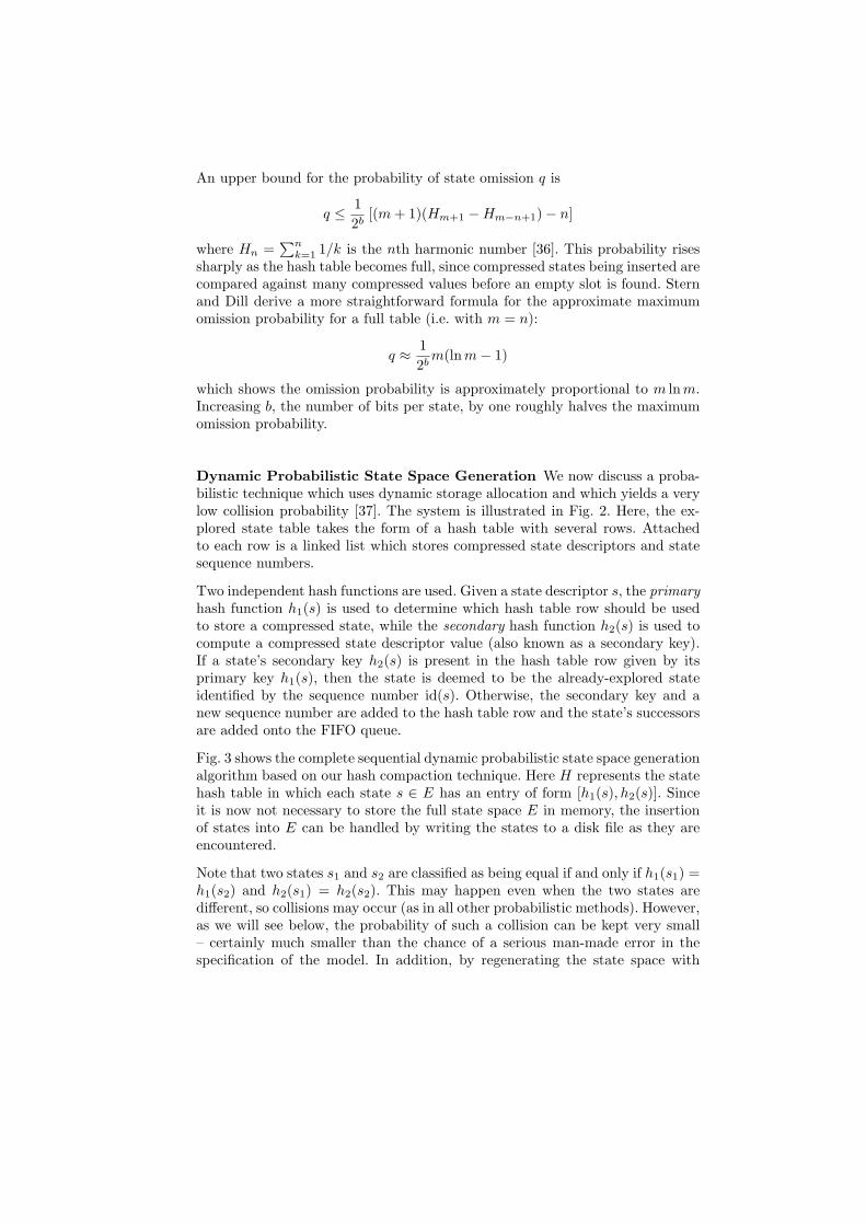
k=1 1/k is the nth harmonic number [36]. This probability risessharply as the hash table becomes full, since compressed states being inserted arecompared against many compressed values before an empty slot is found. Sternand Dill derive a more straightforward formula for the approximate maximumomission probability for a full table (i.e. with m = n):

q ≈ 12b

m(lnm− 1)

which shows the omission probability is approximately proportional to m ln m.Increasing b, the number of bits per state, by one roughly halves the maximumomission probability.

Dynamic Probabilistic State Space Generation We now discuss a proba-bilistic technique which uses dynamic storage allocation and which yields a verylow collision probability [37]. The system is illustrated in Fig. 2. Here, the ex-plored state table takes the form of a hash table with several rows. Attachedto each row is a linked list which stores compressed state descriptors and statesequence numbers.

Two independent hash functions are used. Given a state descriptor s, the primaryhash function h1(s) is used to determine which hash table row should be usedto store a compressed state, while the secondary hash function h2(s) is used tocompute a compressed state descriptor value (also known as a secondary key).If a state’s secondary key h2(s) is present in the hash table row given by itsprimary key h1(s), then the state is deemed to be the already-explored stateidentified by the sequence number id(s). Otherwise, the secondary key and anew sequence number are added to the hash table row and the state’s successorsare added onto the FIFO queue.

Fig. 3 shows the complete sequential dynamic probabilistic state space generationalgorithm based on our hash compaction technique. Here H represents the statehash table in which each state s ∈ E has an entry of form [h1(s), h2(s)]. Sinceit is now not necessary to store the full state space E in memory, the insertionof states into E can be handled by writing the states to a disk file as they areencountered.

Note that two states s1 and s2 are classified as being equal if and only if h1(s1) =h1(s2) and h2(s1) = h2(s2). This may happen even when the two states aredifferent, so collisions may occur (as in all other probabilistic methods). However,as we will see below, the probability of such a collision can be kept very small– certainly much smaller than the chance of a serious man-made error in thespecification of the model. In addition, by regenerating the state space with

2h (s ) id(s )

2h (s ) id(s ) 2h (s ) id(s ) 2h (s ) id(s ) 2h (s ) id(s )0 0 3 3 6 6 7 7

31118156 50604823 43591640 735761000 3 6 7

2h (s ) id(s )2h (s ) id(s )4 4 8 8

71685177 162487114 8

1id(s )

ih (s )1

primaryhash key

secondaryhash keys

2h (s )i

2h (s ) id(s ) 2h (s ) id(s )0

2

1 5 5

08783635 1 5r-1

1

etc.

2h (s )

2 2 9 9

98318241 402368972 9 10

id(s )h (s )2

29949409

62703471

10 10

Fig. 2. Layout of the explored state table under the dynamic probabilistic hash com-paction scheme

beginH = {[h1(s0), h2(s0)]}F .add(s0)E = { s0 }A = ∅while (F not empty) do begin

F .remove(s)for each s′ ∈ succ(s) do begin

if [h1(s′), h2(s′)] /∈ H do beginF .add(s′)E = E ∪ {s′}H = H ∪ {[h1(s′), h2(s′)]}

endA = A ∪ {id(s) → id(s′)}

endend

end

Fig. 3. Sequential dynamic probabilistic state space generation algorithm

different sets of independent hash functions and comparing the resulting numberof states and transitions, it is possible to further arbitrarily decrease the risk ofan undetected collision.

We now calculate the probability of complete state coverage p. We consider ahash table with r rows and t = 2b possible secondary key values, where b is thenumber of bits used to store the secondary key. In such a hash table, there are rtpossible ways of representing a state. Assuming that h1(s) and h2(s) distributestates randomly and independently, each of these representations are equallylikely. Thus, if there are n distinct states to be inserted into the hash table, theprobability p that all states are uniquely represented is given by:

p =(rt)!

(rt− n)!(rt)n(24)

An equivalent formulation of Eq. (24) is:

p =n−1∏

i=0

rt− i

rt=

n−1∏

i=0

(1− i

rt

)(25)

Assuming n ¿ rt and using the fact that ex ≈ (1 + x) for |x| ¿ 1, we obtain:

p ≈n−1∏

i=0

e−i/rt = ePn−1

i=0 −i/rt = e−n(n−1)

2rt = en−n22rt

Since n2 À n for large n, a simple approximation for p is given by:

p ≈ e−n22rt (26)

It can be shown that if n2 ¿ rt then this approximation is also a lower boundfor p (and thus provides a conservative estimate for the probability of completestate coverage) [10].

The corresponding upper bound for the probability q that all states are notuniquely represented, resulting in the omission of one or more states from thestate space, is of course simply:

q = 1− p ≤ n2

2rt=

n2

r2b+1. (27)

Thus the probability of state omission q is proportional to n2 and is inverselyproportional to the hash table size r. Increasing the size of the compressed statedescriptors b by one bit halves the omission probability.

1

0.1

0.01

0.001

0.0001

1e-05

1e-06

1e-07

1e-08

1e-09

1e-101 10 100 1000 10000 100000 1e+06 1e+07 1e+08

omis

sion

pro

babi

lity

number of states

holzmannwolper and leroy

stern and dilldynamic hash

Fig. 4. Contemporary static probabilistic methods compared with the dynamic hashcompaction method in terms of omission probability

Method Parameters Method Parameters

Holzmann l = 7.488× 109 bits Wolper b = 42 bitsM = 91.4 MB and s = 32 bits

Leroy m = 108 slotsM = 91.6 MB

Method Parameters Method Parameters

Stern b = 40 bits b = 40 bitsand s = 32 bits Dynamic s = 32 bitsDill m = 10.26× 108 slots hash r = 6 000 000 rows

M = 91.4 MB h = 6 bytesM = 91.4 MB(for n = 108)

Table 1. Parameters used in the comparison of omission probabilities

Comparison of State Omission Probabilities Fig. 4 compares the omis-sion probability of contemporary static probabilistic methods with that of thedynamic hash compaction method for state space sizes of various magnitudesup to 108. The parameters used for each method are presented in Tab. 1, andare selected such that the memory use of all four algorithms is the same. Thegraph shows that the dynamic method yields a far lower omission probabilitythan both Holzmann’s method and Wolper and Leroy’s method. In addition,the dynamic method is competitive with Stern and Dill’s algorithm and yieldsa better omission probability when the hash table becomes full or nearly full.

Parallel Dynamic Probabilistic State Space Generation We now inves-tigate how our technique can be enhanced to take advantage of the memory andprocessing power provided by a network of workstations or a distributed-memoryparallel computer. We assume there are N nodes available and that each pro-cessor has its own local memory and can communicate with other nodes via anetwork.

In the parallel algorithm, the state space is partitioned between the nodes sothat each node is responsible for exploring a portion of the state space andfor constructing part of the state graph. A partitioning hash function h0(s) →(0, . . . , N − 1) is used to assign states to nodes, such that node i is responsiblefor exploring the set of states Ei and for constructing the portion of the stategraph Ai where:

Ei = {s : h0(s) = i}Ai = {(s1 → s2) : h0(s1) = i}

It is important that h0(s) achieves a good spread of states across nodes in orderto achieve good load balance. Naturally, the values produced by h0(s) should alsobe independent of those produced by h1(s) and h2(s) to enhance the reliabilityof the algorithm. Guidelines for choosing hash functions which meet these goalsare discussed in [10].

The operation of node i in the parallel algorithm is shown in Fig. 5. Each nodei has a local FIFO queue Fi used to hold unexplored local states and a hashtable Hi representing a compressed version of the set Ei, i.e. those states whichhave been explored locally. State s is assigned to processor h0(s), which storesthe state’s compressed state descriptor h2(s) in the local hash table row givenby h1(s). As before, it is not necessary to store the complete state space Ei inmemory, since states can be written out to a disk file as they are encountered.

Node i proceeds by removing a state from the local FIFO queue and determiningthe set of successor states. Successor states for which h0(s) = i are dealt withlocally, while other successor states are sent to the relevant remote processorsvia calls to send-state(k, g, s). Here k is the remote node, g is the identity of theparent state and s is the state descriptor of the child state. The remote processors

beginif h0(s0) = i do begin

Hi = {[h1(s0), h2(s0)]}Fi.add(s0)Ei = {s0}

end elseHi = Ei = ∅

Ai = ∅while (shutdown signal not received) do begin

if (Fi not empty) do begins = Fi.remove()for each s′ ∈ succ(s) do begin

if h0(s′) = i do beginif [h1(s′), h2(s′)] /∈ Hi do begin

Hi = Hi ∪ {[h1(s′), h2(s′)]}Fi.add(s′)Ei = Ei ∪ {s′}

endAi = Ai ∪ {id(s) → id(s′)}

end elsesend-state(h0(s′), id(s), s′)

endendwhile (receive-id(g, h)) do

Ai = Ai ∪ {g → h}while (receive-state(k, g, s′)) do begin

if [h1(s′), h2(s′)] /∈ Hi do beginHi = Hi ∪ {h1(s′), h2(s′)}Fi.add(s′)Ei = Ei ∪ {s′}

endsend-id(k, g, id(s′))

endend

end

Fig. 5. Parallel state space generation algorithm for node i

s’

parent state

child state

sh (s)0Node

0h (s’)Node

1

2

1h (s’) 2h (s’)[ , ] if in H

1h (s’) 2h (s’)[ , ] insert into H

lookup id(s’)

push s’ onto stack Fissue id(s’)

else do begin

end

3

0h (s)

0h (s’)

0h (s)

0h (s’)

state s’to node

sends

node node

id(s’)from node

receives

Fig. 6. Steps required to identify child state s′ of parent s.

must receive incoming states via matching calls to receive-state(k, g, s) wherek is the sender node. If they are not already present, the remote processor addsthe incoming states to both the remote state hash table and FIFO queue.

For the purpose of constructing the state graph, states are identified by a pairof integers (i, j) where i = h0(s) is the node number of the host processor andj is the local state sequence number. As in the sequential case, the index j canbe stored in the state hash table of node i. However, a node will not be aware ofthe state identity numbers of non-local successor states. Therefore, when a nodereceives a state it returns its identity to the sender by calling send-id(k, g, h)where k is the sender, g is the identity of the parent state and h is the identityof the received state. The identity is received by the original sender via a callto receive-id(g, h). Fig. 6 summarises the main steps that take place to identifyand process each child s′ of state s in the case that h0(s) 6= h0(s′).

In practice, it is inefficient to implement the communication as detailed in Fig. 5and Fig. 6, since the network rapidly becomes overloaded with too many shortmessages. Consequently state and identity messages are buffered and sent inlarge blocks. In order to avoid starvation and deadlock, nodes that have veryfew states left in their FIFO queue or are idle broadcast a message to othernodes requesting them to flush their outgoing message buffers.

The algorithm terminates when all the Fi are empty and there are no outstandingstate or identity messages. The problem of determining when these conditionsare satisfied across a distributed set of processes is a non-trivial problem. From

the several distributed termination algorithms surveyed in [38], we have chosento use Dijkstra’s circulating probe algorithm [39].

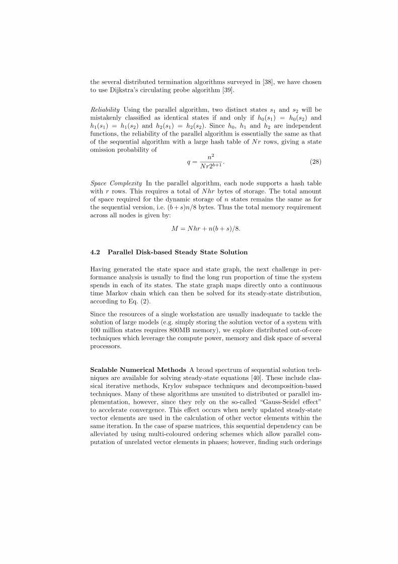
Reliability Using the parallel algorithm, two distinct states s1 and s2 will bemistakenly classified as identical states if and only if h0(s1) = h0(s2) andh1(s1) = h1(s2) and h2(s1) = h2(s2). Since h0, h1 and h2 are independentfunctions, the reliability of the parallel algorithm is essentially the same as thatof the sequential algorithm with a large hash table of Nr rows, giving a stateomission probability of

q =n2

Nr2b+1. (28)

Space Complexity In the parallel algorithm, each node supports a hash tablewith r rows. This requires a total of Nhr bytes of storage. The total amountof space required for the dynamic storage of n states remains the same as forthe sequential version, i.e. (b+ s)n/8 bytes. Thus the total memory requirementacross all nodes is given by:

M = Nhr + n(b + s)/8.

4.2 Parallel Disk-based Steady State Solution

Having generated the state space and state graph, the next challenge in per-formance analysis is usually to find the long run proportion of time the systemspends in each of its states. The state graph maps directly onto a continuoustime Markov chain which can then be solved for its steady-state distribution,according to Eq. (2).

Since the resources of a single workstation are usually inadequate to tackle thesolution of large models (e.g. simply storing the solution vector of a system with100 million states requires 800MB memory), we explore distributed out-of-coretechniques which leverage the compute power, memory and disk space of severalprocessors.

Scalable Numerical Methods A broad spectrum of sequential solution tech-niques are available for solving steady-state equations [40]. These include clas-sical iterative methods, Krylov subspace techniques and decomposition-basedtechniques. Many of these algorithms are unsuited to distributed or parallel im-plementation, however, since they rely on the so-called “Gauss-Seidel effect”to accelerate convergence. This effect occurs when newly updated steady-statevector elements are used in the calculation of other vector elements within thesame iteration. In the case of sparse matrices, this sequential dependency can bealleviated by using multi-coloured ordering schemes which allow parallel com-putation of unrelated vector elements in phases; however, finding such orderings

CG

Classical ConjugateGradient algorithm

(for SPD A)

CGS

(Bi)Conjugate GradientSquared

BiCGSTAB

(Bi)Conjugate GradientSquared Stabilised

BiCGSTAB(L)

using normal equations(residual minimizing)

Conjugate Gradient

CGNR CGNE

using normal equations(error minimizing)

Conjugate Gradient

CG appliedto AA’

CG appliedto A’A

BiCG

Biconjugate Gradients(for non−symmetric A)

GMRES

GeneralisedMinimal RESidual

(for nonsymmetric A)

QMR

Quasi−MinimalResidual

TFQMR

Transpose−freeQuasi−Minimal

Residual

1−dimensional localresidual minimization

L−dimensional localresidual minimization

(Bi)Conjugate GradientSquared Stabilisedwith L−dimensional

residual minimization

quasi−optimal least−squares minimization

of residual

QMR smoothing ofCGS auxiliary

sequence

uses short recurrencesto generate orthogonal

basis for symmetric matrix A

uses short recurrencesto generate biorthogonal

basis for arbitrary matrix A

uses long recurrencesto generate orthogonal

basis for arbitrary matrix A

residualpolynomialsquared

reformedresidual

polynomial

better residualpolynomialallowing

complex roots

Symmetric Lanczos Non−symmetric Lanczos Arnoldi Process

CG applied to double system

Conjugate Krylov Subspace methods

Generalized CG methods

Basis−generating algorithms

Fig. 7. An overview of Krylov subspace techniques

is a combinatorial problem of exponential complexity. Consequently obtainingsuitable orderings for very large matrices is infeasible.

Most classical iterative methods, such as Gauss-Seidel and Successive Overre-laxation (SOR), suffer from this problem. An important exception is the Jacobimethod which uses independent updates of vector elements. The Jacobi methodis characterised by slow, smooth convergence.

Krylov subspace methods [41] are a powerful class of iterative methods whichincludes many conjugate gradient-type algorithms. They derive their name fromthe fact that they generate their iterates using a shifted Krylov subspace asso-ciated with the coefficient matrix. They are widely used in scientific comput-ing since they are parameter free (unlike SOR) and exhibit rapid, if somewhat

erratic, convergence. In addition, these methods are well suited to parallel im-plementation because they are based on matrix–vector products, independentvector updates and inner products. Fig. 7 presents a conceptual overview ofthe most important techniques. The arrows show the relationships between themethods, i.e. how the methods have been generalised from their underlying basis-generating algorithms and also how key concepts have been inherited from onealgorithm to the next.

The most recently developed Krylov subspace algorithms (such as CGS [42],BiCGSTAB [43] and TFQMR [44]) are also particularly suited to a disk-basedimplementation since they access A in a predictable fashion and do not re-quire multiplication with AT . Compared to classical iterative methods, however,Krylov subspace techniques have high memory requirements. CGS is often usedbecause it requires the least memory of these methods.

Disk-based Solution Techniques The concept of using magnetic disk as abuffer to store data that is too large to fit into main memory is an idea whichoriginated three decades ago with the development of overlays and virtual mem-ory systems. However, only recently, with the widespread availability of large,cheap, high-bandwidth hard disks has attention been focused on the potentialof disks as high-throughput data sources appropriate for use in data-intensivecomputations.

In [45] and [46], Deavours and Sanders make a compelling case for the potentialof disk-based steady-state solution methods for large Markov models. They notethat our ability to solve large matrices is limited by the memory required tostore a representation of the transition matrix and by the effective rate at whichmatrix elements can be produced from the encoding. As a general rule, the morecompact the representation, the more CPU overhead is involved in retrievingmatrix elements. Two common encodings are Kronecker representations and “on-the-fly” methods. Deavours and Sanders estimate the effective data productionrate of Kronecker and “on-the-fly” methods as being 2 MB/s and 440 KB/srespectively on their 120 MHz HP C110 workstation. Other published resultsshow that an implementation of a state-of-the-art Kronecker technique runningon a 450 MHz Pentium-II workstation yields an effective data production rateof around 2.5 MB/s [27].

At the same time, modern workstation disks are capable of sustaining datatransfer rates in excess of 20 MB/s. This suggests that it would be worthwhileto store the transition matrix on disk, given that enough disk space is availableand given that we can apply an iterative solution method that accesses thetransition matrix in a predictable way. Such an approach has the potential toproduce data faster than both Kronecker and on-the-fly methods, without anyof the structural restrictions inherent in Kronecker methods.

LocalDisk

LocalDisk

Local

LocalDisk

Disk

Process

Disk I/O

Compute Disk I/O

SharedMemory

Compute

Shared SharedMemory

MemoryShared

Process

ProcessDisk I/O Compute

Process

Memory

ProcessCompute

Process

ProcessProcess

Disk I/O

Network

Buffer 1

Buffer 2

Buffer 1

Buffer 2

Semaphores

P0

P2Semaphores

Buffer 1

Buffer 2

SemaphoresP3

Buffer 1

Buffer 2

P1

Semaphores

Fig. 8. Distributed disk-based solver architecture

Deavours and Sanders demonstrate the effectiveness of this approach by devis-ing a sequential disk-based solution tool which makes use of two cooperatingprocesses. One of the processes is dedicated to reading disk data while the otherperforms computation using a Block Gauss-Seidel algorithm, thus allowing forthe overlap of disk I/O and computation. The processes communicate usingsemaphores and shared memory. The advantage of using Block Gauss-Seidel isthat diagonal matrix blocks can be read from disk once, be cached in memoryand then reused several times.

The memory required by the disk-based approach is small – besides the sharedmemory buffers, space is only required for the solution vector itself. This enablesthe solution of extremely large models with over 10 million states and 100 millionnon-zero entries on a HP C110 workstation with 128MB RAM and 4GB of diskspace in just over 5 hours.

Kwiatkowska and Mehmood reduce the memory requirements of disk-basedmethods even further by proposing a block-based Gauss-Seidel method whichuses disk to store blocks of the steady-state vector as well as matrix blocks [47,48]. In this way, a model of a manufacturing system with 133 million states issolved on a single PC in 13 days and 9 hours.

Parallel disk-based solver architectures have also been implemented with somesuccess. Fig. 8 shows the architecture proposed in [49]. Each node has two pro-cesses: a Disk I/O process dedicated to reading matrix elements from a localdisk, and a Compute process which performs the iterations using a Jacobi orCGS-based matrix–vector multiply kernel. The processes share two data bufferslocated in shared memory and synchronise via semaphores. Together the pro-

cesses operate as a classical producer-consumer system, with the disk I/O processfilling one shared memory buffer while the compute process consumes data fromthe other.

Bell and Haverkort apply a similar architecture in solving a 724 million stateMarkov chain model on a 26 node PC cluster in 16 days [50].

1 2 3 4 5 6 7 8 9 10 11 12 13 14 15 16

1

2

3

4

5

6

7

8

9

10

11

12

13

14

15

16

13 7 16 10 15 9 1 3 14 8 11 4 2 12 5 6

P1

P2

P3

P4

13

7

16

10

15

9

1

3

14

8

11

4

2

12

5

6

x

Fig. 9. A 16 × 16 non-symmetric sparse matrix (left), with corresponding 4-way hy-pergraph partition (right) and corresponding partitions of the vector

Hypergraph Partitioning Any distributed solution scheme involves partition-ing the sparse matrix and vector elements across the processors. Such schemesnecessitate the exchange of data (vector elements and possibly partial sums)after every iteration in the solution process. The objective in partitioning thematrix is to minimise the amount of data which needs to be exchanged whilebalancing the computational load (as given by the number of non-zero elementsassigned to each processor).

Hypergraph partitioning is an extension of graph partitioning. Its primary appli-cation to date has been in VLSI circuit design, where the objective is to clusterpins of devices such that interconnect is minimised. It can also be applied to theproblem of allocating the non-zero elements of sparse matrices across processorsin parallel computation [51].

Formally, a hypergraph H = (V,N ) is defined by a set of vertices V and a setof nets (or hyperedges) N , where each net is a subset of the vertex set V [51].In the context of a row-wise decomposition of a sparse matrix A, matrix row i(1 ≤ i ≤ n) is represented by a vertex vi ∈ V while column j (1 ≤ j ≤ n) isrepresented by net Nj ∈ N . The vertices contained within net Nj correspondto the row numbers of the non-zero elements within column j, i.e. vi ∈ Nj if

0

1000

2000

3000

4000

5000

0 1000 2000 3000 4000 5000

0

1000

2000

3000

4000

5000

0 1000 2000 3000 4000 5000

P1

P2

P3

P4

x

Fig. 10. Transposed transition matrix (left) and corresponding hypergraph-partitionedmatrix (right)

and only if aij 6= 0. The weight of vertex i is given by the number of non-zeroelements in row i, while the weight of a net is its contribution to the edge cut,which is defined as one less than the number of different partitions spanned bythat net. The overall objective of a hypergraph sparse matrix partitioning is tominimise the sum of the weights of the cut nets while maintaining a balancecriterion. A column-wise decomposition is achieved in an analogous fashion.

The matrix on the right of Fig. 9 shows the result of applying hypergraph-partitioning to the matrix on the left in a four-way row-wise decomposition.Although the number of off-diagonal non-zeros is 18 the number of vector ele-ments which must be transmitted between processors during each matrix–vectormultiplication (the communication cost) is 6. This is because the hypergraph par-titioning algorithms not only aim to concentrate the non-zeros on the diagonalsbut also strive to line up the off-diagonal non-zeros in columns. The edge cut ofthe decomposition is also 6, and so the hypergraph partitioning edge cut metricexactly quantifies the communication cost. This is a general property and oneof the key advantages of using hypergraphs – in contrast to graph partitioning,where the edge cut metric merely approximates communication cost. Optimalhypergraph partitioning is NP-complete but there are a small number of hyper-graph partitioning tools which implement fast heuristic algorithms, for examplePaToH [51], hMeTiS [52] and Parkway [53].

Fig. 10 shows the application of hypergraph partitioning to a (transposed) gen-erator matrix. Statistics about the communication associated with this decom-position for a single matrix–vector multiplication are presented in Tab. 2. Wesee that around 90% of the non-zero elements allocated to each processor arelocal, i.e. they are multiplied with vector elements that are stored locally. The

proc- non- local remote reusedessor zeros % % % 1 2 3 4

1 7 022 99.96 0.04 0 1 - 407 - 42 7 304 91.41 8.59 34.93 2 3 - 16 1813 6 802 88.44 11.56 42.11 3 - - - 124 6 967 89.01 10.99 74.28 4 - 1 439 -

Table 2. Communication overhead (left) and interprocessor communication matrix(right).

remote non-zero elements are multiplied with vector elements that are sent fromother processors. However, because the hypergraph decomposition tends to alignremote non-zero elements in columns (well illustrated in the 2nd block belongingto processor 4), reuse of received vector elements is good (up to 74%) with cor-respondingly lower communication overhead. The communication matrix on theright in Tab. 2 shows the number of vector elements sent between each pair ofprocessors during each iteration (e.g. 181 vector elements are sent from processor2 to processor 4).

4.3 Parallel Computation of Densities and Quantiles of FirstPassage Time

A rapid response time is an important performance criterion for almost allcomputer-communication and transaction processing systems. Response timequantiles are frequently specified as key quality of service metrics in ServiceLevel Agreements and industry standard benchmarks such as TPC. Examplesof systems with stringent response time requirements include mobile commu-nication systems, stock market trading systems, web servers, database servers,flexible manufacturing systems, communication protocols and communicationnetworks. Typically, response time targets are specified in terms of quantiles –for example “95% of all text messages must be delivered within 3 seconds”.

In the past, numerical computation of analytical response time densities hasproved prohibitively expensive except in some Markovian systems with restrictedstructure such as overtake-free queueing networks [54]. However, with the adventof high-performance parallel computing and the widespread availability of PCclusters, direct numerical analysis on Markov and semi-Markov chains has nowbecome a practical proposition.

There are two main methods for computing first passage time (and hence re-sponse time) densities in Markov chains: those based on Laplace transforms andtheir inversion [55, 56] and those based on uniformisation [8, 6]. The former haswider application to semi-Markov processes but is less efficient than uniformisa-tion when restricted to Markov chains.

Numerical Laplace Transform Inversion The key to practical analysis ofsemi-Markov processes lies in the efficient representation of their general distri-butions. Without care the structural complexity of the SMP can be recreatedwithin the representation of the distribution functions.

Many techniques have been used for representing arbitrary distributions – two ofthe most popular being phase-type distributions and vector-of-moments methods.These methods suffer from, respectively, exploding representation size undercomposition, and containing insufficient information to produce accurate answersafter large amounts of composition.

As all our distribution manipulations take place in Laplace-space, we link ourdistribution representation to the Laplace inversion technique that we ultimatelyuse. Our tool supports two Laplace transform inversion algorithms, which arebriefly outlined below: the Euler technique [57] and the Laguerre method [58]with modifications summarised in [59].

Both algorithms work on the same general principle of sampling the transformfunction L(s) at n points, s1, s2, . . . , sn and generating values of f(t) at m user-specified t-points t1, t2, . . . , tm. In the Euler inversion case n = km, where k canvary between 15 and 50, depending on the accuracy of the inversion required. Inthe modified Laguerre case, n = 400 and, crucially, is independent of m.

The process of selecting a Laplace transform inversion algorithm is discussedlater; however, whichever is chosen, it is important to note that calculatingsi, 1 ≤ i ≤ n and storing all our distribution transform functions, sampled atthese points, will be sufficient to provide a complete inversion. Key to this isthat fact that matrix element operations, of the type performed in Eq. (39), (i.e.convolution and weighted sum) do not require any adjustment to the array ofdomain s-points required. In the case of a convolution, for instance, if L1(s) andL2(s) are stored in the form {(si, Lj(si)) : 1 ≤ i ≤ n}, for j = 1, 2, then theconvolution, L1(s)L2(s), can be stored using the same size array and using thesame list of domain s-values, {(si, L1(si)L2(si)) : 1 ≤ i ≤ n}.Storing our distribution functions in this way has three main advantages. Firstly,the function has constant storage space, independent of the distribution-type.Secondly, each distribution has, therefore, the same constant storage require-ment even after composition with other distributions. Finally, the function hassufficient information about a distribution to determine the required passagetime (and no more).

Summary of Euler Inversion The Euler method is based on the Bromwich con-tour inversion integral, expressing the function f(t) in terms of its Laplace trans-form L(s). Making the contour a vertical line s = a such that L(s) has nosingularities on or to the right of it gives:

f(t) =2eat

π

∫ ∞

0

Re(L(a + iu)) cos(ut) du (29)

This integral can be numerically evaluated using the trapezoidal rule with step-size h = π/2t and a = A/2t (where A is a constant that controls the discretisationerror), which results in the nearly alternating series:

f(t) ≈ fh(t) =eA/2

2tRe(L(A/2t)) +

eA/2

2t

∞∑

k=1

(−1)kRe(

L

(A + 2kπi

2t

))(30)

Euler summation is employed to accelerate the convergence of the alternatingseries infinite sum, so we calculate the sum of the first n terms explicitly anduse Euler summation to calculate the next m. To give an accuracy of 10−8 weset A = 19.1, n = 20 and m = 12 (compared with A = 19.1, n = 15 and m = 11in [57]).

Summary of Laguerre Inversion The Laguerre method [58] makes use of theLaguerre series representation:

f(t) =∞∑

n=0

qnln(t) : t ≥ 0 (31)

where the Laguerre polynomials ln are given by:

ln(t) =(

2n− 1− t

n

)ln−1(t)−

(n− 1

n

)ln−2(t) (32)

starting with l0 = et/2 and l1 = (1− t)et/2, and:

qn =1

2πrn

∫ π

0

Q(reiu)e−iru du (33)

where r = (0.1)4/n and Q(z) = (1− z)−1L((1 + z)/2(1− z)).

The integral in the calculation of qn can be approximated numerically by thetrapezoidal rule, giving:

qn ≈ qn =1

2nrn

Q(r) + (−1)nQ(−r) + 2

n−1∑

j=1

(−1)jRe(Q(reπji/n)

) (34)

As described in [59], the Laguerre method can be modified by noting that theLaguerre coefficients qn are independent of t. This means that if the number oftrapezoids used in the evaluation of qn is fixed to be the same for every qn (ratherthan depending on the value of n), values of Q(z) (and hence L(s)) can be reusedafter they have been computed. Typically, we set n = 200. In order to achievethis, however, the scaling method described in [58] must be used to ensure thatthe Laguerre coefficients have decayed to (near) 0 by n = 200. If this can beaccomplished, the inversion of a passage time density for any number of t-values

can be achieved at the fixed cost of calculating 400 truncated summations ofthe type shown in Eq. (39). This is in contrast to the Euler method, where thenumber of truncated summations required is a function of the number of pointsat which the value of f(t) is required.

Iterative Passage-Time Analysis for SMPs Passage-time analysis in semi-Markov processes involves the solution of a set of linear equations in complexvariables. In [60], we set out an efficient iterative approach to passage timecalculation and proved its convergence to the analytic passage time distribution.The algorithm has since been implemented and is used to calculate semi-Markovpassage times in the SMARTA tool (described below).

Recall the semi-Markov process, Z(t), of Sect. 2.2, where N(t) is the numberof state transitions that have taken place by time t. We formally define the rthtransition first passage time to be:

P(r)ij = inf{u > 0 : Z(u) ∈ j, N(u) > 0 | N(u) ≤ r, Z(0) = i} (35)

which is the time taken to enter a state in j for the first time having startedin state i at time 0 and having undergone up to r state transitions1. P

(r)ij is a

random variable with associated Laplace transform, L(r)ij (s). L

(r)ij (s) is, in turn,

the ith component of the vector:

L(r)j (s) = (L(r)

1j (s), L(r)2j (s), . . . , L(r)

Nj(s)) (36)

representing the passage time for terminating in j for each possible start state.This vector may be computed as:

L(r)j (s) = U(I + U′ + U′2 + · · ·+ U′(r−1)) ej (37)

where U is a matrix with elements upq = r∗pq(s) and U′ is a modified version ofU with elements u′pq = δp6∈j upq, where states in j have been made absorbing.We include the initial U-transition in Eq. (37), so as to generate cycle times forcases such as L

(r)ii (s) which would otherwise register as 0 if U′ were used instead.

The column vector ej has entries ekj = δk∈j .

From Eq. (15) and Eq. (35):

Pij = P(∞)ij and thus Lij(s) = L

(∞)ij (s) (38)

We can generalise to multiple source states i using the normalised steady-statevector α of Eq. (21):

L(r)ij (s) = αL(r)

j (s)=

∑r−1k=0 αUU′k ej

(39)

1 If there are immediate transitions in the semi-Markov process then we have to use amodified formulation of the passage time and iterative passage time definitions [60].

The sum of Eq. (39) can be computed efficiently using sparse matrix–vectormultiplications with a vector accumulator, µr =

∑rk=0 αUU′k. At each step,

the accumulator (initialised as µ0 = αU) is updated with µr+1 = αU + µrU′.

The worst-case time complexity for this sum is O(N2r) versus the O(N3) oftypical matrix inversion techniques. In practice, for a sparse matrix with constantbandwidth (number of non-zeros per row), this can be as low as O(Nr).

DTMCSteadyState

Solver

DistributedLaplace

TransformInverter

Hypergraph

Partitioner

masterprocessor

LT inverterwith no

L(s)evaluation

masterdisk

cachefilter

disk cachemaster

partitionedmatrixfiles

EnhancedDNAmacahigh−level

specification GeneratorSpaceState

s1

s2

LT inverter

L(s)evaluation

with

L(s )1

L(s )n

memory cachemaster

L(s )2

L(s )2

L(s )1 L(s )

1

L(s )n

memory cachemaster

L(s )2

s−value work queues−values

groupsslave processor

Fig. 11. Parallel hypergraph-based passage time density calculation pipeline

The SMARTA Tool Our iterative passage-time analysis algorithm has beenimplemented in the SMARTA tool [61], the architecture of which is shown inFig. 11. The process of calculating a passage time density begins with a high-levelmodel specified in an enhanced form of the DNAmaca interface language [62,10]. This language supports the specification of stochastic Petri nets, queueingnetworks and stochastic process algebras. Next, a probabilistic, hash-based stategenerator [37] uses the high-level model description to produce the transitionprobability matrix P of the model’s embedded Markov chain, the matrices Uand U′, and a list of the initial and target states. Normalised weights for the

initial states are determined by the solution of π = πP, which is readily doneusing any of a variety of steady-state solution techniques (e.g. [45, 49]). U′ isthen partitioned using a hypergraph partitioning tool (a single partitioning issufficient since all linear systems to be solved have the same non-zero structure).

Control is then passed to the distributed passage time density calculator, whichis implemented in C++ using the Message Passing Interface (MPI) [63] standard.This employs a master-slave architecture with groups of slave processors. Themaster processor computes in advance the values of s at which it will need toknow the value of Lij(s) in order to perform the inversion. This can be doneirrespective of the inversion algorithm employed. The s-values are then placedin a global work-queue to which the groups of slave processors make requests.

The highest ranking processor in a group of slaves makes a request to the masterfor an s-value and is assigned the next one available. This is then broadcast tothe other members of the slave group to allow them to construct their columnsof the matrix U′ for that specific s. Each processor reads in the columns of thematrix U′ that correspond to its allocated partition into two types of sparsematrix data structure and also reads in the initial source-state weighting vectorα. Local non-zero elements (i.e. those elements in diagonal matrix blocks thatwill be multiplied with vector elements stored locally) are stored in a conven-tional compressed sparse column format. Remote non-zero elements (i.e. thoseelements in off-diagonal matrix blocks that must be multiplied with vector ele-ments received from other processors) are stored in an ultrasparse matrix datastructure – one for each remote processor – using a coordinate format. Eachprocessor then determines which vector elements need to be received from andsent to every other processor in the group on each iteration, adjusting the rowindices in the ultrasparse matrices so that they index into a vector of receivedelements. This ensures that a minimum amount of communication takes placeand makes multiplication of off-diagonal blocks with received vector elementsefficient.

For each step in our iterative algorithm, each processor begins by using non-blocking communication primitives to send and receive remote vector elements,while calculating the product of local matrix elements with locally stored vectorelements. The use of non-blocking operations allows computation and commu-nication to proceed concurrently on parallel machines where dedicated networkhardware supports this effectively. The processor then waits for the completionof non-blocking operations (if they have not already completed) before multiply-ing received remote vector elements with the relevant ultrasparse matrices andadding their contributions to the local vector-matrix product cumulatively.

Once the calculations of a slave group are deemed to have converged, the result isreturned to the master by the highest-ranking processor in the group and cached.When all results have been computed and returned for all required values of s,the final Laplace inversion calculations are made by the master, resulting in therequired t-points.

5 Application examples

We demonstrate our analysis techniques on three application examples: a GSPNmodel of a communications protocol, a SM-SPN model of a voting system anda PEPA model of an active badge system.

5.1 Courier Protocol Model

Description The GSPN shown in Fig. 12 (originally presented in [64]) modelsthe ISO Application, Session and Transport layers of the Courier sliding-windowcommunication protocol. Data flows from a sender (p1 to p26) to a receiver(p27 to p46) via a network. The sender’s transport layer fragments outgoingdata packets; this is modelled as two paths between p13 and p35. The pathvia t8 carries all fragments before the last one through the network to p33.Acknowledgements for these fragments are sent back to the sender (as signalledby the arrival of a token on p20), but no data is delivered to the higher layerson the receiver side. The path via t9 carries the last fragment of each messageblock. Acknowledgements for these fragments are generated and a data token isdelivered to higher receiver layers via t27.

The average number of data packets sent is determined by the ratio of the weightson the immediate transitions t8 and t9. This ratio, known as the fragmentationratio, is given by q1 : q2 (where q1 and q2 are the weights associated with transi-tions t8 and t9 respectively). Thus, this number of data packets is geometricallydistributed, with parameter q1/(q1 + q2). Here we use a fragmentation ratio ofone.

The transport layer is further characterised by two important parameters: thesliding window size n (p14) and the transport space m (p17). Different values ofm and n yield state spaces of various sizes. The transition rates r1, r2, . . . , r10have the same relative magnitudes as those obtained by benchmarking a workingimplementation of the protocol (see [64]).

State Space Generation We have implemented the state generation algo-rithm of Fig. 5 on a Fujitsu AP3000 distributed memory parallel computer.Our implementation is written in C++ with support for two popular parallelprogramming interfaces, viz. the Message Passing Interface (MPI) [65] and theParallel Virtual Machine (PVM) interface [66]. The generator uses hash tableswith r = 750 019 rows per processor and b = 40 bit secondary keys. The resultswere collected using up to 16 processors on the AP3000. Each processor has a300MHz UltraSPARC processor, 256MB RAM and a 4GB local disk. The nodesrun the Solaris operating system and support MPI. They are connected by ahigh-speed wormhole-routed network with a peak throughput of 65MB/s.

n

courier1

networkdelay

senderapplication

task

sendersession

task

sendertransport

task

receiverapplication

task

receiversession

task

receivertransport

task

m

p2

t2

p4p3

p5

p6

p8

t5

p10 p9

p11

p13p12

p16p15

p14

p17

p20 p18 p19

t14t13

p22p21t15

p23

p24 p25

p26

p27 p28 p29

t23 t24

p31p30

p32

t22

p33 p34

t27

p35

p36 p37

t29

p38 p39

p40

p41

p42

t32

p44p43

p45 p46p1

courier3courier2

courier4

network delay

t1 (r7)

t3 (r1)

t4 (r2)

t6 (r1)

t7 (r8)

t12 (r3)

t8 (q1) t9 (q2)

t11 (r5)t10 (r5)

t18 (r4)

t16 (r6) t17 (r6)

t34 (r10)

t33 (r1)

t31 (r2)

t30 (r1)

t28 (r9)

t25 (r5) t26 (r5)

t19 (r3) t20 (r4) t21 (r4)

Fig. 12. The Courier Protocol Software Generalised Stochastic Petri net [64].

k n a

1 11 700 48 3302 84 600 410 1603 419 400 2 281 6204 1 632 600 9 732 3305 5 358 600 34 424 2806 15 410 250 105 345 9007 39 836 700 286 938 6308 94 322 250 710 223 930

1

10

100

1000

10000

100000

1e+06

1e+07

1e+08

1e+09

1e+10

1 2 3 4 5 6 7 8k

tangible states (n)arcs in state graph (a)

Fig. 13. The number of tangible states (n) and the number of arcs (a) in the stategraph of the Courier model for various values of k.

The Courier model features a scaling parameter k (corresponding to the slidingwindow size) which we will vary to produce state graphs of different sizes (seeFig. 13).

The graph on the left of Fig. 14 shows the distributed run-time taken to exploreCourier state spaces of various sizes (up to k = 6) using 1, 2, 4, 8, 12 and 16processors on the AP3000. Each observed value is calculated as the mean offour runs. The k = 5 state space (5 358 600 states) can be generated on a singleprocessor in 16 minutes 20 seconds; 16 processors require only 89 seconds. Thek = 6 state space (15 410 250 states) can be generated on a single processor in51 minutes 45 seconds; 16 processors require just 267 seconds.

The corresponding speedups for the cases k = 1, 2, 3, 4, 5, 6 are shown in thegraph on the right of Fig. 14. For k = 6 using 16 processors, we observe aspeedup of 11.65, giving an efficiency of 73%.

Memory utilisation is low – a single processor generating the k = 5 state spaceuses a total of 91MB (17.4 bytes per state), while the k = 6 state space requires175MB (11.6 bytes per state). This is far less than the 94 bytes per state (4516-bit integers plus a 32-bit unique state indentifier) that would be required bya straightforward exhaustive implementation.

Moving beyond the maximum state space size that can be generated on a singleprocessor, on 16 processors we find that the k = 7 state space can be generatedin around 10 minutes while just under 26 minutes are required to generate thek = 8 state space (with 94 322 250 states and 710 223 930 arcs).

k=1 k=2 k=3 k=4 k=5 k=6 k=7 k=8

Jacobi time (s) 33.647 278.18 1506.4 5550.3Jacobi iterations 4925 4380 4060 3655

p = 1 CGS time (s) 2.1994 21.622 163.87 934.27 29134CGS iterations 60 81 106 129 157Memory/node (MB) 20.3 22.1 30.5 60.8 154.0

Jacobi time (s) 29.655 176.62 1105.7 4313.6Jacobi iterations 4925 4380 4060 3655

p = 2 CGS time (s) 1.6816 13.119 93.28 509.90 7936.9CGS iterations 57 84 107 131 148Memory/node (MB) 20.2 21.1 25.45 41.2 89.7

Jacobi time (s) 25.294 148.45 627.96 3328.3Jacobi iterations 4925 4380 4060 3655

p = 4 CGS time (s) 1.2647 8.4109 58.302 322.50 1480.5CGS iterations 60 80 108 133 159Memory/node (MB) 20.1 20.6 22.9 31.4 57.5

Jacobi time (s) 38.958 140.06 477.02 1780.9 6585.4Jacobi iterations 4925 4380 4060 3655 3235

p = 8 CGS time (s) 1.4074 6.0976 39.999 204.46 934.76 4258.7CGS iterations 61 82 109 132 155 171Memory/node (MB) 20.0 20.3 21.7 26.5 41.4 81.6

Jacobi time (s) 32.152 133.58 457.23 1559.0 6329.2 11578 72202Jacobi iterations 4925 4380 4060 3655 3235 2325 2190

p = 12 CGS time (s) 1.4973 5.9345 34.001 157.73 852.53 2579.6 21220CGS iterations 58 83 104 129 156 189 180Memory/node (MB) 20.0 20.3 21.3 24.9 36.1 66.2 99.7

Jacobi time (s) 41.831 125.68 506.31 1547.9 5703.4 11683 32329Jacobi iterations 4925 4380 4060 3650 3235 2325 2190

p = 16 CGS time (s) 3.3505 7.1101 31.322 134.48 577.68 2032.5 13786 141383CGS iterations 60 91 104 132 146 173 179 213Memory/node (MB) 20.0 20.2 21.0 24.1 33.4 58.5 79.8 161

Table 3. Real time in seconds required for the distributed solution of the Couriermodel.

Steady-state Analysis Tab. 3 presents the execution time (defined as max-imum processor run-time) in seconds required for the distributed disk-basedsolution of models using the CGS and Jacobi methods. The models range in sizefrom k = 1 (11 700 states) to k = 7 (39.8 million states) and runs are conductedon 1, 2, 4, 8, 12 and 16 processors. The number of iterations for convergence andmemory use per processor are also shown.

Fig. 15 compares the convergence of the Jacobi method with that of the CGSalgorithm for the k = 4 case in terms of the number of matrix multiplicationsperformed. As is typical for many models, the Jacobi method begins by converg-ing quickly, but then plateaus, converging very slowly but smoothly. The CGS

algorithm, on the other hand, exhibits erratic rapid convergence that improvesin a concave fashion.

The largest state space solved is the k = 8 case (94 million states) which takes1 day 15 hours of processing time on 16 processors. The total amount of I/Oacross all nodes is 3.4TB, with the nodes jointly processing an average of 24MBdisk data every second.

k = 1 k = 2 k = 3 k = 4 k = 5 k = 6 k = 7 k = 8

λ 74.3467 120.372 150.794 172.011 187.413 198.919 207.690 214.477Psend 0.01011 0.01637 0.02051 0.02334 0.02549 0.02705 0.02825 0.02917Precv 0.98141 0.96991 0.96230 0.95700 0.95315 0.95027 0.94808 0.94638Psess1 0.00848 0.01372 0.01719 0.01961 0.02137 0.02268 0.02368 0.02445Psess2 0.92610 0.88029 0.84998 0.82883 0.81345 0.80196 0.79320 0.78642Ptransp1 0.78558 0.65285 0.56511 0.50392 0.45950 0.42632 0.40102 0.38145Ptransp2 0.78871 0.65790 0.57138 0.51084 0.46673 0.43365 0.40835 0.38871

Table 4. Courier Protocol performance measures in terms of the transport windowsize k.

Using the steady state vector, it is straightforward to derive some simple resource-based performance measures, as shown in Tab. 4. The most important is λ, thedata throughput rate, which is given by the throughput of transition t21. Othermeasures yield task utilizations. In particular, Ptransp1 = Pr{p12 is marked} =Pr{transport task 1 is idle}. Similarly we define Ptransp2 for p32, Psess1 andPsess2 using p6 and p41, and Psend and Precv using p1 and p46.

First Passage Time Analysis We now apply our iterative passage-time anal-ysis technique to determine the end-to-end response time from the initiationof a transport layer transmission to the arrival of the corresponding acknowl-edgement packet. Consequently we choose as source markings those markingsfor which M(p11) > 0, and as destination markings those markings for whichM(p20) > 0. This approach works easily for a sliding window size of n = 1since there can be only one outstanding unacknowledged packet. Naturally, if wewished to calculate the response time for sliding window sizes greater than one,we would need to augment the state vector used to describe markings to trackthe progress of a particular token through the Petri net.

The underlying reachability graph contains 29 010 markings, 11 700 of which aretangible and 17 310 of which are vanishing. There are 7 320 source markings and1 680 destination markings. Fig. 16 shows the resulting numerical response timedensity. The median (50% quantile) and 95% quantile transmission times arealso given. Once again the numerical results are compared against a simulation,and agreement is excellent.

0

500

1000

1500

2000

2500

3000

3500

0 2e+06 4e+06 6e+06 8e+06 1e+07 1.2e+071.4e+071.6e+07

time

(sec

onds

)

tangible states generated

1 processor 2 processors 4 processors 8 processors12 processors16 processors

1

2

3

4

5

6

7

8

9

10

11

12

13

14

15

16

1 2 3 4 5 6 7 8 9 10 11 12 13 14 15 16

spee

dup

number of processors

k=1k=2k=3k=4k=5k=6

Fig. 14. Real time taken to generate Courier state spaces up to k = 6 using theoriginal algorithm on 1, 2, 4, 8, 12 and 16 processors (left), and the resulting speedupsfor k = 1, 2, 3, 4, 5 and 6 (right).

-10

-9

-8

-7

-6

-5

-4

-3

-2

-1

0

1

0 50 100 150 200 250 300 350 400 450 500

log1

0(re

sidu

al n

orm

/vec

tor

norm

)

matrix-vector multiplications

cgsjacobi

Fig. 15. Jacobi and CGS convergence behaviour for the Courier model with k = 4

0

0.005

0.01

0.015

0.02

0.025

0.03

0 20 40 60 80 100

Pro

babi

lity

dens

ity

Time

Result from 10 simulation runs of 1 billion transitions eachUniformization result

Laplace result

Fig. 16. Numerical and simulated response time densities for time taken from theinitiation of a transport layer transmission (i.e. those markings for which M(p11) > 0)to the arrival of an acknowledgement packet (i.e. those markings for which M(p20) > 0).The median response time (50% quantile) is 0.0048 seconds, and the 95% quantile is0.0114 seconds.

For this example, our Laguerre scaling algorithm selected a damping parame-ter of σ = 0.008. A single slave (a 1.4GHz Athlon processor with 256MB RAM)required 24 minutes 15 seconds to calculate the 200 points plotted on the numer-ical passage time density graph. Using 8 slave PCs with the same configurationdecreased the required time to just 3 minutes 23 seconds (corresponding to anefficiency of 96%). 16 slave PCs required 2 minutes 17 seconds (72% efficiency).These results reflect the excellent scalability of our approach.

5.2 Voting Model

Description Fig. 17 represents a voting system with CC voters, MM pollingunits and NN central voting servers. In this system, voters cast votes throughpolling units which in turn register votes with all available central voting units.Both polling units and central voting units can suffer breakdowns, from whichthere is a soft recovery mechanism. If, however, all the polling or voting unitsfail, then, with high priority, a failure recovery mode is instituted to restore thesystem to an operational state.

We demonstrate the SMP passage-time analysis techniques of the previous sec-tions with a large semi-Markov model of a distributed voting system (Fig. 17).

Fig. 17. A semi-Markov stochastic Petri net of a voting system with breakdowns andrepairs

The model is specified in a semi-Markov stochastic Petri net (SM-SPN) for-malism [67] using an extension of the DNAmaca Markov chain modelling lan-guage [62].

The distributions are specified directly as Laplace transforms with certain macrosprovided for popular distributions (e.g. uniform, gamma, deterministic) and canbe made marking dependent by use of the m(pi) function (which returns thecurrent number of tokens at place, pi). Support for inhibiting transitions is alsoprovided.

For the voting system, Tab. 5 shows how the size of the underlying SMP variesaccording to the configuration of the variables CC, MM , and NN .

First Passage Time Analysis The results presented in this section wereproduced on a Beowulf Linux cluster with 64 dual processor nodes, a maximumof 34 of which can be used by a single job. Each node has two Intel Xeon 2.0GHzprocessors and 2GB of RAM. The nodes are connected by a Myrinet networkwith a peak throughput of 250 Mb/s.

Table 5. Different configurations of the voting system and state space generated

System CC MM NN States

1 60 25 4 106 5402 100 30 4 249 7603 125 40 4 541 2804 150 40 5 778 8505 175 45 5 1 140 0506 300 80 10 10 999 140

0

0.002

0.004

0.006

0.008

0.01

0.012

500 550 600 650 700 750 800

Pro

babi

lity

dens

ity

Time

Passage time density: 10.9 million state voting modelError from 10 simulation runs of 1 billion transitions each

Fig. 18. Analytic and simulated (with 95% confidence intervals) density for the timetaken to process 300 voters in the voting model system 6 (10.9 million states).

0

0.2

0.4

0.6

0.8

1

500 550 600 650 700 750 800

Cum

ulat

ive

prob

abili

ty

Time

Cumulative passage time distribution: 10.9 million state voting model

Fig. 19. Cumulative distribution function and quantile of the time taken to process300 voters in the voting model system 6 (10.9 million states).

We display passage time densities produced by the iterative passage time algo-rithm and also by simulation to validate those results.

Fig. 18 shows the density of the time taken to process 300 voters (as given bythe passage of 300 tokens from place p1 to p2) in system 6 of the voting model.Calculation of the analytical density required 15 hours and 7 minutes using 64slave processors (in 8 groups of 8) for the 31 t-points plotted. Our algorithmevaluated Lij(s) at 1 023 s-points, each of which involved manipulating sparsematrices of rank 10 999 140. The analytical curve is validated against the com-bined results from 10 simulations, each of which consisted of 1 billion transitionfirings. Despite this large simulation effort, we still observe wide confidence in-tervals (probably because of the rarity of source states).

Fig. 19 is a cumulative distribution for the same passage as Fig. 18 (easilyobtained by inverting Lij(s)/s from cached values of Lij(s)). It allows us toextract response time quantiles, for instance:

IP(system 6 can process 300 voters in less than 730 seconds) = 0.9876

5.3 PEPA Active Badge Model

Description In the original active badge model, described in [68], there are 4rooms on a corridor, all installed with active badge sensors, and a single personwho can move from one room to an adjacent room. The sensors are linked to

Person1 = (reg1, r).Person1 + (move2, m).Person2

Personi = (movei−1, m).Personi−1 + (reg i, r).Personi

+ (movei+1, m).Personi+1

: 1 < i < NPersonN = (moveN−1, m).PersonN−1 + (regN , r).PersonN

Sensor i = (reg i,>).(repi, s).Sensor i : 1 ≤ i ≤ N

Dbasei =PN

j=1(repj ,>).Dbasej : 1 ≤ i ≤ N

Sys =QM

j=1 Person1 ¤¢Reg

QNj=1 Sensor j ¤¢

RepDbase1

where Reg = {reg i | 1 ≤ i ≤ N} and Rep = {repi | 1 ≤ i ≤ N}

Fig. 20. The PEPA description for the generalised active badge model with N roomsand M people.

a database which records which sensor has been activated last. In the model ofFig. 20, we have M people in N rooms with sensors and a database that canbe in one of N states. To maintain a reasonable state space, this is a simpledatabase which does not attempt to keep track of every individual’s location;rather it remembers the last movement that was made by any person in thesystem.

In the model below, Personi represents a person in room i, Sensor i is the sensorin room i and Dbasei is the state of the database. A person in room i can eithermove to room i − 1 or i + 1 or, if they remain there long enough, set off thesensor in room i, which registers its activation with the database.

The first thing to note about such a model is how fast the state space can grow.With M people in N rooms, we already have NM states just from the differentconfigurations of people in rooms. Then there are 2N sensor configurations andfinally N states that the database can be in, giving us a total of 2NNM+1 states.For as few as 3 people and 6 rooms, the example we use, we have a global statespace of 82, 944 states.

First Passage Time Analysis We include two passages from the active badgesystem with 3 people and 6 possible rooms. As the model of Fig. 20 tells us, all6 people start in room 1 and move out from there.

Fig. 21 shows the density function for the passage representing how long it takesfor all 3 people to be together in room 6 for the first time.

It is interesting to observe that it is virtually impossible for all 3 people to endup in room 6, which requires 6 successive move transitions from all 3 people for

0

0.0002

0.0004

0.0006

0.0008

0.001

0.0012

0.0014

0.0016

0 50 100 150 200

Pro

babi

lity

dens

ity, p

Time, t

Passage: 3 people in R1 to 3 people in R6

Fig. 21. The passage time density for 3 people starting in room 1 ending up all inroom 6.

0

0.005

0.01

0.015

0.02

0.025

0.03

0 20 40 60 80 100 120 140

Pro

babi

lity

dens

ity, p

Time, t

Passage: 3 people in R1 any 1 person in R6

Fig. 22. The passage time density for 3 people starting in room 1 ending up with anyone or more of them in room 6.

it to happen at the earliest opportunity, until at least 10 time units have elapsed.After that time, very low probabilities are registered and the distribution clearlyhas a very heavy tail.

0

0.2

0.4

0.6

0.8

1

0 20 40 60 80 100 120 140

Pro

babi

lity,

p

Time, t

Passage: 3 people in R1 any 1 person in R6

Fig. 23. The cumulative passage time distribution function for 3 people starting inroom 1 ending up with any one or more of them in room 6.

The second passage of Fig. 22 shows an equivalent passage time density from thesame start point to a terminating condition of at least one person of the threeentering room 6. The resulting passage is much less heavy tailed, as this timeonly a single person has to make it to room 6 before the passage ends.

From these densities, it is a simple matter to construct cumulative distributionfunctions (the integral of the density function) and obtain quantiles, e.g. theprobability that 3 people all reach room 6 by time t = 150. Fig. 23 shows thecumulative distribution function (cdf) corresponding to the passage time densityof Fig. 22. From this cdf, we can ascertain, for example, that there is a 90%probability that at least one person will have reached room 6 by time t = 62.

6 Conclusion and Future Perspectives

Performance analysis of complex systems is a computationally expensive activ-ity. If a model does not have exploitable symmetries or other structure thatallows for analytical or numerical shortcuts to be used, then an explicit repre-sentation of the state space has to be constructed. This chapter has discussedsome state space generation methods and numerical algorithms for steady-stateand passage-time analysis of (semi-)Markov models which are scalable acrosslarge computing clusters. We have shown that by making use of probabilisticalgorithms and efficient distribution strategies (e.g. using hypergraph partition-

ing), we can subdivide large performance analysis problems in such a way thatmakes them tractable on individual computer nodes.

An important emerging development with the potential to tackle exceptionallylarge state spaces is the use of continuous approximations to represent largediscrete state spaces. Preliminary efforts to relate this to modelling formalismshave led to continuous state-space translations from SPNs [69] and PEPA [70].In both cases, repeated structures in the top-level formalism are represented bysystems of ordinary differential equations (ODEs) which describe a deterministictrace of behaviour. In certain structural situations [71] the steady-state solutionof the ODEs corresponds to the steady-state solution of the underlying Markovchain.

Acknowledgements

The authors would like to thank Nicholas Dingle, Peter Harrison and AleksandarTrifunovic who contributed hugely to the development of the work presented hereand without whom this would not have been possible.

References

1. J. Yang, C. Sar, and D. Engler, “eXplode: a Lightweight, General System forFinding Serious Storage System Errors,” in Proc. 7th Symposium on OperatingSystem Design and Implementation, (Seattle, WA), pp. 131–146, November 2006.

2. F. Bause and P. Kritzinger, Stochastic Petri Nets – An Introduction to the Theory.Wiesbaden, Germany: Verlag Vieweg, 1995.

3. W. Grassman, “Means and variances of time averages in Markovian environments,”European Journal of Operational Research, vol. 31, no. 1, pp. 132–139, 1987.

4. A. Reibman and K. Trivedi, “Numerical transient analysis of Markov models,”Computers and Operations Research, vol. 15, no. 1, pp. 19–36, 1988.

5. G. Bolch, S. Greiner, H. Meer, and K. Trivedi, Queueing Networks and MarkovChains. Wiley, August 1998.

6. B. Melamed and M. Yadin, “Randomization procedures in the computation ofcumulative-time distributions over discrete state Markov processes,” OperationsResearch, vol. 32, pp. 926–944, July–August 1984.

7. A. Miner, “Computing response time distributions using stochastic Petri nets andmatrix diagrams,” in Proceedings of the 10th International Workshop on PetriNets and Performance Models (PNPM’03), (Urbana-Champaign, IL), pp. 10–19,September 2nd–5th 2003.

8. J. Muppala and K. Trivedi, “Numerical transient analysis of finite Markovianqueueing systems,” in Queueing and Related Models (U. Bhat and I. Basawa, eds.),pp. 262–284, Oxford University Press, 1992.

9. M. Ajmone-Marsan, G. Conte, and G. Balbo, “A class of Generalised Stochas-tic Petri Nets for the performance evaluation of multiprocessor systems,” ACMTransactions on Computer Systems, vol. 2, pp. 93–122, 1984.

10. W. Knottenbelt, Parallel Performance Analysis of Large Markov Models. PhDthesis, Imperial College London, February 2000.

11. J. T. Bradley, N. J. Dingle, P. G. Harrison, and W. J. Knottenbelt, “Distributedcomputation of passage time quantiles and transient state distributions in largesemi-Markov models,” in PMEO’03, Performance Modelling, Evaluation and Op-timization of Parallel and Distributed Systems, (Nice), p. 281, IEEE ComputerSociety Press, April 2003.

12. C. Hoare, Communicating Sequential Processes. Prentice Hall, 1985.13. R. Milner, Communication and Concurrency. Prentice Hall, 1989.14. J. Hillston, A Compositional Approach to Performance Modelling. PhD thesis,

University of Edinburgh, 1994.15. M. Rettelbach and M. Siegle, “Compositional minimal semantics for the stochastic

process algebra TIPP,” in Proceedings of the 2nd Workshop on Process Algebrasand Performance Modelling, pp. 31–50, Regensberg/Erlangen: Arbeitsberichte desIMMD, Universitat Erlangen-Nurnberg, July 1994.

16. H. Hermanns and M. Rettelbach, “Syntax, semantics, equivalences and axioms forMTIPP,” in Proceedings of the 2nd Workshop on Process Algebras and Perfor-mance Modelling, Regensberg/Erlangen: Arbeitsberichte des IMMD, UniversitatErlangen-Nurnberg, July 1994.

17. P. Buchholz, “Markovian Process Algebra: composition and equivalence,” in Pro-ceedings of the 2nd Workshop on Process Algebras and Performance Modelling,Regensberg/Erlangen: Arbeitsberichte des IMMD, Universitat Erlangen-Nurnberg,July 1994.

18. M. Bernardo, L. Donatiello, and R. Gorrieri, “Modelling and analyzing concur-rent systems with MPA,” in Proceedings of the 2nd Workshop on Process Algebrasand Performance Modelling, pp. 89–106, Regensberg/Erlangen: Arbeitsberichte desIMMD, Universitat Erlangen-Nurnberg, July 1994.

19. H. Hermanns, U. Herzog, and J. Hillston, “Stochastic process algebras—A formalapproach to performance modelling,” tutorial, Department of Computer Science,University of Edinburgh, Edinburgh EH9 3JZ, UK, 1996.

20. B. Strulo, Process Algebra for Discrete Event Simulation. PhD thesis, ImperialCollege, London, October 1993.

21. P. G. Harrison and B. Strulo, “SPADES - a process algebra for discrete eventsimulation,” Journal of Logic and Computation, vol. 10, pp. 3–42, January 2000.

22. J. T. Bradley, “Semi-Markov PEPA: Modelling with generally distributed actions,”International Journal of Simulation, vol. 6, pp. 43–51, January 2005.

23. M. Bravetti, M. Bernardo, and R. Gorrieri, “Towards performance evaluation withgeneral distributions in process algebras,” in CONCUR’98, Proceedings of the 9thInternational Conference on Concurrency Theory (D. Sangiorgi and R. de Simone,eds.), vol. 1466 of Lecture Notes in Computer Science, pp. 405–422, Springer-Verlag, Nice, September 1998.

24. M. Bravetti and R. Gorrieri, “Interactive generalized semi-Markov processes,” inProcess Algebra and Performance Modelling Workshop (J. Hillston and M. Silva,eds.), pp. 83–98, Centro Politecnico Superior de la Universidad de Zaragoza, Pren-sas Universitarias de Zaragoza, Zaragoza, September 1999.

25. J. Hillston and M. Ribaudo, “Stochastic process algebras: a new approach to per-formance modelling,” in Modelling and Simulation of Advanced Computer Systems(K. Bagchi and G. Zobrist, eds.), ch. 10, pp. 235–256, Gordon Breach, 1998.

26. R. Bryant, “Graph-based algorithms for Boolean function manipulation,” IEEETransactions on Computers, vol. C-35, pp. 677–691, August 1986.

27. G. Ciardo and A. Miner, “A data structure for the efficient Kronecker solutionof GSPNs,” in Proceedings of the 8th International Conference on Petri Nets andPerformance Models (PNPM’99), (Zaragoza, Spain), pp. 22–31, IEEE ComputerSociety Press, September 1999.

28. A. Miner and D. Parker, “Symbolic representations and analysis of large proba-bilistic systems,” in Lecture Notes in Computer Science 2925/2004: Validation ofStochastic Systems, pp. 296–338, 2004.

29. P. Buchholz and P. Kemper, “Kronceker based matrix representations for largeMarkov models,” in Lecture Notes in Computer Science 2925/2004: Validation ofStochastic Systems, pp. 256–295, 2004.

30. M. Rabin, “Probabilistic algorithm for testing primality,” Journal of Number The-ory, vol. 12, pp. 128–138, 1980.

31. M. Kuntz and K. Lampka, “Probabilistic meothds in state space analysis,” inLecture Notes in Computer Science 2925/2004: Validation of Stochastic Systems,pp. 339–383, 2004.

32. G. Holzmann, Design and Validation of Computer Protocols. Prentice-Hall, 1991.33. G. Holzmann, “An analysis of bitstate hashing,” in Proceedings of IFIP/PSTV95:

Conference on Protocol Specification, Testing and Verification, Warsaw, Poland:Chapman & Hall, June 1995.

34. B. Bloom, “Space/time trade-offs in hash coding with allowable errors,” Commu-nications of the ACM, vol. 13, pp. 422–426, July 1970.

35. P. Wolper and D. Leroy, “Reliable hashing without collision detection,” in LectureNotes in Computer Science 697, pp. 59–70, Springer Verlag, 1993.

36. U. Stern and D. Dill, “Improved probabilistic verification by hash compaction,”in IFIP WG 10.5 Advanced Research Working Conference on Correct HardwareDesign and Verification Methods, 1995.

37. W. J. Knottenbelt, P. G. Harrison, M. S. Mestern, and P. S. Kritzinger, “A proba-bilistic dynamic technique for the distributed generation of very large state spaces,”Performance Evaluation, vol. 39, pp. 127–148, February 2000.

38. M. Raynal, Distributed Algorithms and Protocols. John Wiley and Sons, 1988.39. E. Dijkstra, W. Feijen, and A. Gasteren, “Derivation of a termination detection

algorithm for distributed computations.,” Information Processing letters, vol. 16,pp. 217–219, June 1983.

40. W. Stewart, Introduction to the Numerical Solution of Markov Chains. PrincetonUniversity Press, 1994.

41. R. Weiss, “A theoretical overview of Krylov subspace methods,” Applied NumericalMathematics, vol. 19, pp. 207–233, 1995. Special Issue on Iterative Methods forLinear Equations.

42. P. Sonneveld, “CGS, a fast Lanczos-type solver for nonsymmetric linear systems,”SIAM Journal on Scientific and Statistical Computing, vol. 10, pp. 36–52, January1989.

43. H. Vorst, “Bi-CGSTAB: A fast and smoothly converging variant of BiCG for thesolution of nonsymmetric linear systems,” SIAM Journal on Scientific and Statis-tical Computing, vol. 13, pp. 631–644, March 1992.

44. R. Freund, “A transpose-free quasi-minimal residual algorithm for non-Hermitianlinear systems,” SIAM Journal on Scientific Computing, vol. 14, pp. 470–482,March 1993.

45. D. D. Deavours and W. H. Sanders, “An efficient disk-based tool for solving verylarge Markov models,” in TOOLS 1997, Computer Performance Evaluation: Mod-elling Techniques and Tools, vol. 1245 of Lecture Notes in Computer Science, (St.Malo), pp. 58–71, Springer-Verlag, June 1997.

46. D. Deavours and W. Sanders, “An efficient disk-based tool for solving large Markovmodels,” Performance Evaluation, vol. 33, pp. 67–84, June 1998.

47. M. Kwiatkowska and R. Mehmood, “Out-of-core solution of large linear systems ofequations arising from stochastic modelling,” in Proceedings of Process Algebra andPerformance Modelling (PAPM’02), (Copenhagen), pp. 135–151, July 25th–26th2002.

48. R. Mehmood, “Serial disk-based analysis of large stochastic models,” in LectureNotes in Computer Science 2925/2004: Validation of Stochastic Systems, pp. 230–255, 2004.

49. W. J. Knottenbelt and P. G. Harrison, “Distributed disk-based solution techniquesfor large Markov models,” in NSMC’99, Proceedings of the 3rd Intl. Conference onthe Numerical Solution of Markov Chains, (Zaragoza), pp. 58–75, September 1999.

50. A. Bell and B. Haverkort, “Serial and parallel out-of-core solution of linear sys-tems arising from Generalised Stochastic Petri Nets,” in Proc. High PerformanceComputing Symposium (HPC 2001), pp. 242–247, 2001.

51. U. Catalyurek and C. Aykanat, “Hypergraph-partitioning-based decomposition forparallel sparse-matrix vector multiplication,” IEEE Transactions on Parallel andDistributed Systems, vol. 10, pp. 673–693, July 1999.

52. G. Karypis and V. Kumar, hMETIS: A Hypergraph Partitioning Package, Version1.5.3. University of Minnesota, November 1998.

53. A. Trifunovic and W. Knottenbelt, “Parkway 2.0: A parallel multilevel hypergraphpartitioning tool,” in Proceedings of the 19th International Symposium on Com-puter and Information Sciences (ISCIS’04), (Antalya, Turkey), October 27th–29th2004.

54. P. G. Harrison, “Laplace transform inversion and passage-time distributions inMarkov processes,” Journal of Applied Probability, vol. 27, pp. 74–87, March 1990.

55. J. Abate and W. Whitt, “The Fourier-series method for inverting transforms ofprobability distributions,” Queueing Systems, vol. 10, no. 1, pp. 5–88, 1992.

56. P. G. Harrison and W. Knottenbelt, “Passage time distributions in large Markovchains,” in Proceedings of ACM SIGMETRICS 2002, (Marina Del Rey, California),pp. 77–85, June 2002.

57. J. Abate and W. Whitt, “Numerical inversion of Laplace transforms of probabilitydistributions,” ORSA Journal on Computing, vol. 7, no. 1, pp. 36–43, 1995.

58. J. Abate, G. L. Choudhury, and W. Whitt, “On the Laguerre method for nu-merically inverting Laplace transforms,” INFORMS Journal on Computing, vol. 8,no. 4, pp. 413–427, 1996.

59. P. G. Harrison and W. J. Knottenbelt, “Passage-time distributions in large Markovchains,” in Proceedings of ACM SIGMETRICS 2002 (M. Martonosi and E. A. deSouza e Silva, eds.), pp. 77–85, Marina Del Rey, USA, June 2002.

60. J. T. Bradley, N. J. Dingle, W. J. Knottenbelt, and H. J. Wilson, “Hypergraph-based parallel computation of passage time densities in large semi-Markov models,”Journal of Linear Algebra and Applications, vol. 386, pp. 311–334, July 2004.

61. N. Dingle, Parallel Computation of Response Time Densities and Quantiles inLarge Markov and Semi-Markov Models. PhD thesis, Imperial College London,October 2004.

62. W. Knottenbelt, “Generalised Markovian analysis of timed transition systems,”Master’s thesis, University of Cape Town, Cape Town, South Africa, July 1996.

63. W. Gropp, E. Lusk, and A. Skjellum, Using MPI: Portable Parallel Programmingwith the Message Passing Interface. Cambridge, Massachussetts: MIT Press, 1994.

64. C. Woodside and Y. Li, “Performance Petri net analysis of communication protocolsoftware by delay-equivalent aggregation,” in Proceedings of the 4th InternationalWorkshop on Petri nets and Performance Models (PNPM’91), (Melbourne, Aus-tralia), pp. 64–73, IEEE Computer Society Press, 2–5 December 1991.

65. W. Gropp, E. Lusk, and A. Skjellum, Using MPI: Portable Parallel Programmingwith the Message Passing Interface. Cambridge, Massachussetts: MIT Press, 1994.

66. A. Geist, A. Beguelin, J. Dongarra, W. Jiang, R. Manchek, and V. Sunderam, PVMParallel Virtual Machine: A Users’ Guide and Tutorial for Networked ParallelComputing. Cambridge, Massachussetts: MIT Press, 1994.

67. J. T. Bradley, N. J. Dingle, W. J. Knottenbelt, and P. G. Harrison, “Perfor-mance queries on semi-Markov stochastic Petri nets with an extended ContinuousStochastic Logic,” in PNPM’03, Proceedings of Petri Nets and Performance Models(G. Ciardo and W. Sanders, eds.), (University of Illinois at Urbana-Champaign),pp. 62–71, IEEE Computer Society, September 2003.

68. S. Gilmore, J. Hillston, and G. Clark, “Specifying performance measures forPEPA,” in Proceedings of the 5th International AMAST Workshop on Real-Timeand Probabilistic Systems, vol. 1601 of Lecture Notes in Computer Science, (Bam-berg), pp. 211–227, Springer-Verlag, 1999.

69. J. Julvez, E. Jimenez, L. Recalde, and M. Silva, “On observability in timed contin-uous Petri net systems,” in QEST’04, Proceedings of 1st International Conferenceon the Quantitative Evaluation of Systems, (Enschede), pp. 60–69, IEEE ComputerSociety Press, September 2004.

70. J. Hillston, “Fluid flow approximation of PEPA models,” in QEST’05, Proceed-ings of the 2nd International Conference on Quantitative Evaluation of Systems,(Torino), pp. 33–42, IEEE Computer Society Press, September 2005.

71. T. G. Kurtz, “Solutions of ordinary differential equations as limits of pure jumpMarkov processes,” Journal of Applied Probability, vol. 7, pp. 49–58, April 1970.