tài liệu chương trình acca phần f2 study text bpp 2010
DESCRIPTION
Tài liệu chương trình ACCA phần F2 study text bpp 2010TRANSCRIPT

STUDY
TEXT
PAPER F2 MANAGEMENT ACCOUNTING
In this edition approved by ACCA
We ddiscuss the bbest strategies for studying for ACCA exams
We hhighlight the mmost important elements in the syllabus and the kkey skills you will need
We ssignpost how each chapter links to the syllabus and the study guide
We pprovide lots of eexam focus points demonstrating what the examiner will want you to do
We eemphasise key points in regular ffast forward summaries
We ttest your knowledge of what you've studied in qquick quizzes
We eexamine your understanding in our eexam question bank
We rreference all the important topics in our ffull index
BPP's i-Learn and i-Pass products also support this paper.
FOR EXAMS IN DECEMBER 2009 AND JUNE 2010

ii
First edition 2007
Third edition June 2009
ISBN 9780 7517 6362 1 (Previous ISBN 9780 7517 4721 8)
British Library Cataloguing-in-Publication Data A catalogue record for this book is available from the British Library
Published by
BPP Learning Media Ltd BPP House, Aldine Place London W12 8AA
www.bpp.com/learningmedia
Printed in the United Kingdom
Your learning materials, published by BPP Learning Media Ltd, are printed on paper sourced from sustainable, managed forests.
All our rights reserved. No part of this publication may be reproduced, stored in a retrieval system or transmitted, in any form or by any means, electronic, mechanical, photocopying, recording or otherwise, without the prior written permission of BPP Learning Media Ltd.
We are grateful to the Association of Chartered Certified Accountants for permission to reproduce past examination questions. The suggested solutions in the exam answer bank have been prepared by BPP Learning Media Ltd, except where otherwise stated.
©BPP Learning Media Ltd 2009
Contents iii
ContentsPage
IntroductionHow the BPP ACCA-approved Study Text can help you pass vStudying F2 viiThe exam paper and exam formulae sheet viii
Before you begin… are you confident with basic maths? 1
Part A The nature and purpose of cost and management accounting
1 Information for management 23
Part B Cost classification, behaviour and purpose2 Cost classification 413 Cost behaviour 55
Part C Business mathematics and computer spreadsheets
4 Correlation and regression; expected values 715 Spreadsheets 89
Part D Cost accounting techniques 6 Material costs 1137 Labour costs 1378 Overhead and absorption costing 159 9 Marginal and absorption costing 183 10 Process costing 19711 Process costing, joint products and by-products 225 12 Job, batch and service costing 237
Part E Budgeting and standard costing 13 Budgeting 26114 Standard costing 28115 Basic variance analysis 289 16 Further variance analysis 307
Part F Short-term decision-making techniques 17 Cost-volume-profit (CVP) analysis 32318 Relevant costing and decision-making 34319 Linear programming 357
Exam question bank 379
Exam answer bank 399
Index 417
Review form and free prize draw

iv
A note about copyright Dear Customer
What does the little © mean and why does it matter?
Your market-leading BPP books, course materials and elearning materials do not write and update themselves. People write them: on their own behalf or as employees of an organisation that invests in this activity. Copyright law protects their livelihoods. It does so by creating rights over the use of the content.
Breach of copyright is a form of theft – as well being a criminal offence in some jurisdictions, it is potentially a serious breach of professional ethics.
With current technology, things might seem a bit hazy but, basically, without the express permission of BPP Learning Media:
Photocopying our materials is a breach of copyright
Scanning, ripcasting or conversion of our digital materials into different file formats, uploading them to facebook or emailing them to your friends is a breach of copyright
You can, of course, sell your books, in the form in which you have bought them – once you have finished with them. (Is this fair to your fellow students? We update for a reason.) But the ilearns are sold on a single user license basis: we do not supply ‘unlock’ codes to people who have bought them second hand.
And what about outside the UK? BPP Learning Media strives to make our materials available at prices students can afford by local printing arrangements, pricing policies and partnerships which are clearly listed on our website. A tiny minority ignore this and indulge in criminal activity by illegally photocopying our material or supporting organisations that do. If they act illegally and unethically in one area, can you really trust them?

Introduction v
How the BPP ACCA-approved Study Text can help you pass – AND help you with your Practical Experience Requirement!
NEW FEATURE – the PER alert!
Before you can qualify as an ACCA member, you do not only have to pass all your exams but also fulfil a three year practical experience requirement (PER). To help you to recognise areas of the syllabus that you might be able to apply in the workplace to achieve different performance objectives, we have introduced the ‘PER alert’ feature. You will find this feature throughout the Study Text to remind you that what you are learning to pass your ACCA exams is equally useful to the fulfilment of the PER requirement.
Tackling studying
Studying can be a daunting prospect, particularly when you have lots of other commitments. The different features of the text, the purposes of which are explained fully on the Chapter features page, will help you whilst studying and improve your chances of exam success.
Developing exam awareness
Our Texts are completely focused on helping you pass your exam.
Our advice on Studying F2 outlines the content of the paper, the necessary skills the examiner expects you to demonstrate and any brought forward knowledge you are expected to have.
Exam focus points are included within the chapters to provide information about skills that you will need in the exam and reminders of important points within the specific subject areas.
Using the Syllabus and Study Guide
You can find the syllabus, Study Guide and other useful resources for F2 on the ACCA web site:
www.accaglobal.com/students/study_exams/qualifications/acca_choose/acca/fundamentals/ma
The Study Text covers all aspects of the syllabus to ensure you are as fully prepared for the exam as possible.
Testing what you can do
Testing yourself helps you develop the skills you need to pass the exam and also confirms that you can recall what you have learnt.
We include Exam-style Questions – lots of them - both within chapters and in the Exam Question Bank,as well as Quick Quizzes at the end of each chapter to test your knowledge of the chapter content.

vi Introduction
Chapter features Each chapter contains a number of helpful features to guide you through each topic.
Topic list
Topic list Syllabus reference Tells you what you will be studying in this chapter and the relevant section numbers, together with the ACCA syllabus references.
Introduction Puts the chapter content in the context of the syllabus as a whole.
Study Guide Links the chapter content with ACCA guidance.
Exam Guide Highlights how examinable the chapter content is likely to be and the ways in which it could be examined.
Summarises the content of main chapter headings, allowing you to preview and review each section easily.
Examples Demonstrate how to apply key knowledge and techniques.
Key terms Definitions of important concepts that can often earn you easy marks in exams.
Exam focus points Provide information about skills you will need in the exam and reminders of important points within the specific subject area.
Formula to learn Formulae that are not given in the exam but which have to be learnt.
This is a new feature that gives you a useful indication of syllabus areas that closely relate to performance objectives in your PER.
QuestionGive you essential practice of techniques covered in the chapter.
Case Study Provide real world examples of theories and techniques.
Chapter Roundup A full list of the Fast Forwards included in the chapter,providing an easy source of review.
Quick Quiz A quick test of your knowledge of the main topics in the chapter.
Exam Question Bank Found at the back of the Study Text with more comprehensive chapter questions.
FAST FORWARD

Introduction vii
Studying F2 This paper introduces you to costing and management accounting techniques, including those techniques that are used to make and support decisions. It provides a basis for Paper F5 – PerformanceManagement.
The examiner for this paper is David Forster who was previously the examiner for Paper 1.2 under the previous syllabus. His aims are to test your knowledge of basic costing and management accounting techniques and also to test basic application of knowledge.
1 What F2 is about F2 is one of the three papers that form the Knowledge base for your ACCA studies. Whilst Paper F1 –Accountant in Business gives you a broad overview of the role and function of the accountant, Papers F2 – Management Accounting and F3 – Financial Accounting give you technical knowledge at a fundamental level of the two major areas of accounting. Paper F2 will give you a good grounding in all the basic techniques you need to know in order to progress through the ACCA qualification and will help you with Papers F5 – Performance Management and P5 – Advanced Performance Management in particular.
2 What skills are required? The paper is examined by computer-based exam or a written exam consisting of objective test questions (mainly multiple-choice questions). You are not required, at this level, to demonstrate any written skills.However you will be required to demonstrate the following.
Core knowledge – classification and treatment of costs, accounting for overheads, budgeting and standard costing, decision-making.
Numerical and mathematical skills – regression analysis, linear programming.
Spreadsheet skills – the paper will test your understanding of what can be done with spreadsheets. This section will be particularly useful to you in the workplace.
3 How to improve your chances of passing You must bear the following points in mind.
All questions in the paper are compulsory. This means that you cannot avoid studying any part of the syllabus. The examiner can examine any part of the syllabus and you must be prepared for him to do so.
The best preparation for any exam is to practise lots of questions. Work your way through the Quick Quizzes at the end of each chapter in this Study Text and then attempt the questions in the Exam Question Bank. You should also make full use of the BPP Practice and Revision Kit.
In the exam, read the questions carefully. Beware any question that looks like one you have seen before – it is probably different in some way that you haven’t spotted.
If you really cannot answer something, move on. You can always come back to it.
If at the end of the exam you find you have not answered all of the questions, have a guess. You are not penalised for getting a question wrong and there is a chance you may have guessed correctly. If you fail to choose an answer, you have no chance of getting any marks.

viii Introduction
The exam paper
Format of the paper
Guidance
The exam is a two hour paper that can be taken either as a paper-based or computer-based exam.
There are 50 questions in the paper – 40 questions will be worth two marks each whilst the remaining 10 questions are worth one mark each. There are therefore 90 marks available.
The two mark questions will have a choice of four possible answers (A/B/C/D) whilst the one mark questions will have a choice of two (A/B) or three possible answers (A/B/C). The one and two mark questions will be interspersed and questions will appear in random order (that is, not in Study Guide order). Questions on the same topic will not necessarily be grouped together.
Questions will be a mix of calculation and non-calculation questions in a similar mix to the pilot paper. The pilot paper can be found on the ACCA web site: www.accaglobal.com/students/study_exams/qualifications/acca_choose/acca/fundamentals/ma/past_papers.
The examiner has indicated that the pilot paper is an extremely useful guide to the mix of questions that you might expect to find in the ‘real’ exams. You should therefore study the pilot paper carefully to get an idea of the weighting that each syllabus area will be given in the exam.
Exam formulae sheet You will be given an exam formulae sheet in your exam. This is reproduced below, together with the chapters of the Study Text in which you can find the formulae.
Regression analysis Economic order quantity (Chapter 4 of Study Text) (Chapter 6 of Study Text)
a =n
xbnY
h
0
CDC2
b = 22 )x(xnyxxyn Economic batch quantity
(Chapter 6 of Study Text)
r = ))y(yn)()x(xn(
yxxyn2222
)RD
1(C
DC2
h
0

1
Before you begin … Are you confident with basic maths?

2

Basic maths 3
1 Using this introductory chapter The Paper F2 – Management Accounting syllabus assumes that you have some knowledge of basic mathematics and statistics. The purpose of this introductory chapter is to provide the knowledge required in this area if you haven't studied it before, or to provide a means of reminding you of basic maths and statistics if you are feeling a little rusty in one or two areas!
Accordingly, this introductory chapter sets out from first principles a good deal of the knowledge that you are assumed to possess in the main chapters of the Study Text. You may wish to work right through it now. You may prefer to dip into it as and when you need to. You may just like to try a few questions to sharpen up your knowledge. Don't feel obliged to learn everything in the following pages: they are intended as an extra resource to be used in whatever way best suits you.
2 Integers, fractions and decimals 2.1 Integers, fractions and decimalsAn integer is a whole number and can be either positive or negative. The integers are therefore as follows.
.....,-5, –4, –3, –2, –1, 0, 1, 2, 3, 4, 5..... .
Fractions (such as 1/2, 1/4, 19/35, 101/377, .....) and decimals (0.1, 0.25, 0.3135 .....) are both ways of showing parts of a whole. Fractions can be turned into decimals by dividing the numerator by the denominator (in other words, the top line by the bottom line). To turn decimals into fractions, all you have to do is remember that places after the decimal point stand for tenths, hundredths, thousandths and so on.
2.2 Significant digits Sometimes a decimal number has too many digits in it for practical use. This problem can be overcome by rounding the decimal number to a specific number of significant digits by discarding digits using the following rule.
If the first digit to be discarded is greater than or equal to five then add one to the previous digit. Otherwise the previous digit is unchanged.
2.3 Example: Significant digits (a) 187.392 correct to five significant digits is 187.39
Discarding a 2 causes nothing to be added to the 9.
(b) 187.392 correct to four significant digits is 187.4
Discarding the 9 causes one to be added to the 3.
(c) 187.392 correct to three significant digits is 187
Discarding a 3 causes nothing to be added to the 7.
Question Significant digits
What is 17.385 correct to four significant digits?
Answer17.39

4 Basic maths
3 Mathematical notation 3.1 Brackets Brackets are commonly used to indicate which parts of a mathematical expression should be grouped together, and calculated before other parts. In other words, brackets can indicate a priority, or an order in which calculations should be made. The rule is as follows.
(a) Do things in brackets before doing things outside them.
(b) Subject to rule (a), do things in this order.
(i) Powers and roots (ii) Multiplications and divisions, working from left to right (iii) Additions and subtractions, working from left to right
Thus brackets are used for the sake of clarity. Here are some examples.
(a) 3 + 6 8 = 51. This is the same as writing 3 + (6 8) = 51. (b) (3 + 6) 8 = 72. The brackets indicate that we wish to multiply the sum of 3 and 6 by 8. (c) 12 – 4 2 = 10. This is the same as writing 12 – (4 2) = 10 or 12 – (4/2) = 10. (d) (12 – 4) 2 = 4. The brackets tell us to do the subtraction first.
A figure outside a bracket may be multiplied by two or more figures inside a bracket, linked by addition or subtraction signs. Here is an example.
5(6 + 8) = 5 (6 + 8) = 5 6 + 5 8 = 70
This is the same as 5(14) = 5 14 = 70
The multiplication sign after the 5 can be omitted, as shown here (5(6 + 8)), but there is no harm in putting it in (5 (6 + 8)) if you want to.
Similarly:
5(8 – 6) = 5(2) = 10; or 5 8 – 5 6 = 10
When two sets of figures linked by addition or subtraction signs within brackets are multiplied together, each figure in one bracket is multiplied in turn by every figure in the second bracket. Thus:
(8 + 4)(7 + 2) = (12)(9) = 108 or 8 7 + 8 2 + 4 7 + 4 2 = 56 + 16 + 28 + 8 = 108
3.2 Negative numbers When a negative number (–p) is added to another number (q), the net effect is to subtract p from q.
(a) 10 + (–6) = 10 – 6 = 4 (b) –10 + (–6) = –10 – 6 = –16
When a negative number (-p) is subtracted from another number (q), the net effect is to add p to q.
(a) 12 – (–8) = 12 + 8 = 20 (b) –12 – (–8) = –12 + 8 = –4
When a negative number is multiplied or divided by another negative number, the result is a positive number.
–8 (–4) = +32 –18/(–3) = +6
If there is only one negative number in a multiplication or division, the result is negative.

Basic maths 5
–8 4 = –32 3 (–2) = –6 12/(–4) = –3 –20/5 = –4
Question Negative numbers
Work out the following.
(a) (72 – 8) – (–3 +1)
(b)2
)1129(12
888
(c) 8(2 – 5) – (4 – (–8))
(d)381
10384
3936
Answer(a) 64 – (–2) = 64 + 2 = 66
(b) 8 + (–9) = –1
(c) –24 – (12) = –36
(d) –6 – (–12) – (–27) = –6 + 12 + 27 = 33
3.3 Reciprocals The reciprocal of a number is just 1 divided by that number. For example, the reciprocal of 2 is 1 divided by 2, ie ½.
3.4 Extra symbols You will come across several mathematical signs in this book and there are six which you should learn right away.
(a) > means 'greater than'. So 46 > 29 is true, but 40 > 86 is false. (b) means 'is greater than or equal to'. So 4 3 and 4 4. (c) < means ' is less than'. So 29 < 46 is true, but 86 < 40 is false. (d) means ' is less than or equal to'. So 7 8 and 7 7. (e) means 'is not equal to'. So we could write 100.004 100. (f) means ‘the sum of’.
4 Percentages and ratios 4.1 Percentages and ratios Percentages are used to indicate the relative size or proportion of items, rather than their absolute size. For example, if one office employs ten accountants, six secretaries and four supervisors, the absolutevalues of staff numbers and the percentage of the total work force in each type would be as follows.
Accountants Secretaries Supervisors Total Absolute numbers 10 6 4 20Percentages 50% 30% 20% 100%
6 Basic maths
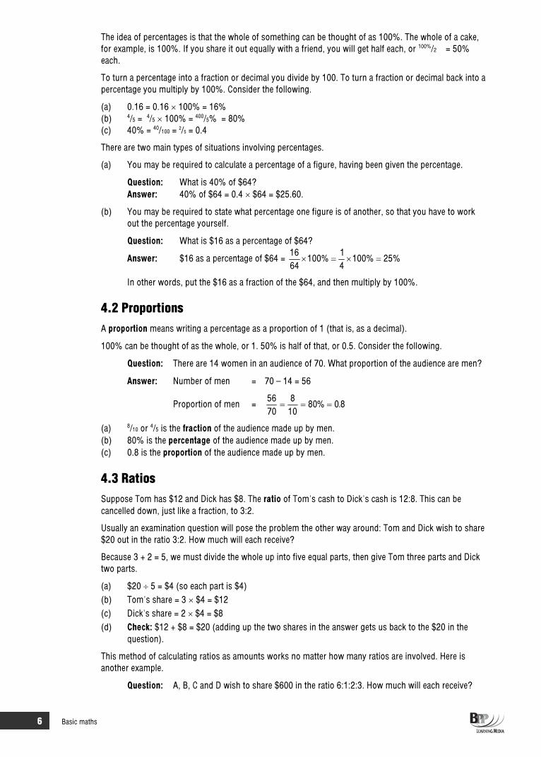
The idea of percentages is that the whole of something can be thought of as 100%. The whole of a cake, for example, is 100%. If you share it out equally with a friend, you will get half each, or 100%/2 = 50% each.
To turn a percentage into a fraction or decimal you divide by 100. To turn a fraction or decimal back into a percentage you multiply by 100%. Consider the following.
(a) 0.16 = 0.16 100% = 16% (b) 4/5 = 4/5 100% = 400/5% = 80% (c) 40% = 40/100 = 2/5 = 0.4
There are two main types of situations involving percentages.
(a) You may be required to calculate a percentage of a figure, having been given the percentage.
Question: What is 40% of $64? Answer: 40% of $64 = 0.4 $64 = $25.60.
(b) You may be required to state what percentage one figure is of another, so that you have to work out the percentage yourself.
Question: What is $16 as a percentage of $64?
Answer: $16 as a percentage of $64 = 25%100%41
100%6416
In other words, put the $16 as a fraction of the $64, and then multiply by 100%.
4.2 ProportionsA proportion means writing a percentage as a proportion of 1 (that is, as a decimal).
100% can be thought of as the whole, or 1. 50% is half of that, or 0.5. Consider the following.
Question: There are 14 women in an audience of 70. What proportion of the audience are men?
Answer: Number of men = 70 – 14 = 56
Proportion of men = 8.0%80108
7056
(a) 8/10 or 4/5 is the fraction of the audience made up by men. (b) 80% is the percentage of the audience made up by men. (c) 0.8 is the proportion of the audience made up by men.
4.3 Ratios Suppose Tom has $12 and Dick has $8. The ratio of Tom's cash to Dick's cash is 12:8. This can be cancelled down, just like a fraction, to 3:2.
Usually an examination question will pose the problem the other way around: Tom and Dick wish to share $20 out in the ratio 3:2. How much will each receive?
Because 3 + 2 = 5, we must divide the whole up into five equal parts, then give Tom three parts and Dick two parts.
(a) $20 5 = $4 (so each part is $4) (b) Tom's share = 3 $4 = $12 (c) Dick's share = 2 $4 = $8 (d) Check: $12 + $8 = $20 (adding up the two shares in the answer gets us back to the $20 in the
question).
This method of calculating ratios as amounts works no matter how many ratios are involved. Here is another example.
Question: A, B, C and D wish to share $600 in the ratio 6:1:2:3. How much will each receive?
Basic maths 7
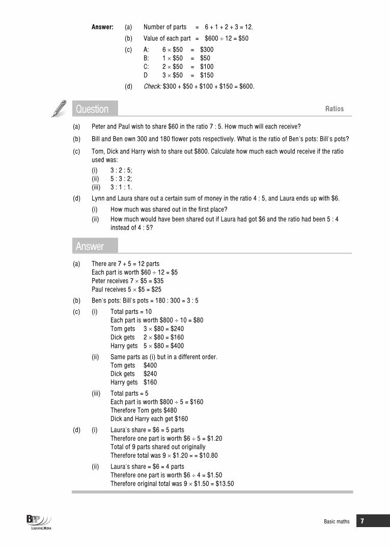
Answer: (a) Number of parts = 6 + 1 + 2 + 3 = 12.
(b) Value of each part = $600 12 = $50
(c) A: 6 $50 = $300 B: 1 $50 = $50 C: 2 $50 = $100 D 3 $50 = $150
(d) Check: $300 + $50 + $100 + $150 = $600.
Question Ratios
(a) Peter and Paul wish to share $60 in the ratio 7 : 5. How much will each receive?
(b) Bill and Ben own 300 and 180 flower pots respectively. What is the ratio of Ben's pots: Bill's pots?
(c) Tom, Dick and Harry wish to share out $800. Calculate how much each would receive if the ratio used was:
(i) 3 : 2 : 5; (ii) 5 : 3 : 2; (iii) 3 : 1 : 1.
(d) Lynn and Laura share out a certain sum of money in the ratio 4 : 5, and Laura ends up with $6.
(i) How much was shared out in the first place? (ii) How much would have been shared out if Laura had got $6 and the ratio had been 5 : 4
instead of 4 : 5?
Answer(a) There are 7 + 5 = 12 parts
Each part is worth $60 12 = $5 Peter receives 7 $5 = $35 Paul receives 5 $5 = $25
(b) Ben's pots: Bill's pots = 180 : 300 = 3 : 5
(c) (i) Total parts = 10 Each part is worth $800 10 = $80 Tom gets 3 $80 = $240 Dick gets 2 $80 = $160 Harry gets 5 $80 = $400
(ii) Same parts as (i) but in a different order. Tom gets $400 Dick gets $240 Harry gets $160
(iii) Total parts = 5 Each part is worth $800 5 = $160 Therefore Tom gets $480 Dick and Harry each get $160
(d) (i) Laura's share = $6 = 5 parts Therefore one part is worth $6 5 = $1.20 Total of 9 parts shared out originally Therefore total was 9 $1.20 = = $10.80
(ii) Laura's share = $6 = 4 parts Therefore one part is worth $6 4 = $1.50 Therefore original total was 9 $1.50 = $13.50

8 Basic maths
5 Roots and powers 5.1 Square roots The square root of a number is a value which, when multiplied by itself, equals the original number.
9 = 3, since 3 3 = 9
Similarly, the cube root of a number is the value which, when multiplied by itself twice, equals the original number.
3 64 = 4, since 4 4 4 = 64
The nth root of a number is a value which, when multiplied by itself (n – 1) times, equals the original number.
5.2 Powers Powers work the other way round.Thus the 6th power of 2 = 26 = 2 2 2 2 2 2 = 64.
Similarly, 34 = 3 3 3 3 = 81.
Since 9 = 3, it also follows that 32 = 9, and since 3 64 = 4, 43 = 64.
When a number with an index (a 'to the power of' value) is multiplied by the same number with the same or a different index, the result is that number to the power of the sum of the indices.
(a) 52 5 = 52 51 = 5(2+1) = 53 = 125 (b) 43 43 = 4(3+3) = 46 = 4,096
Similarly, when a number with an index is divided by the same number with the same or a different index, the result is that number to the power of the first index minus the second index.
(a) 64 63 = 6(4-3) = 61 = 6 (b) 78 76 = 7(8-6) = 72 = 49
Any figure to the power of zero equals one. 10 = 1, 20 = 1, 30 = 1, 40 = 1 and so on.
Similarly, 82 82 = 8(2-2) = 80 = 1
An index can be a fraction, as in 1612 . What 16
12 means is the square root of ).4or16(16 If we multiply
21
16 by 21
16 we get )(
21
21
16 which equals 161 and thus 16.
Similarly, 31
216 is the cube root of 216 (which is 6) because 31
216 31
216 31
216 = )(31
31
31
216
= 2161 = 216.
An index can be a negative value. The negative sign represents a reciprocal. Thus 2-1 is the reciprocal of, or one over, 21
=12
1 =
21
5.3 Example: Roots and powers
(a) 2-2 =221
=41
and 2-3 =32
1 =
81
(b) 5-6 =156
=625,151

Basic maths 9
(c) 45 4-2 = 4524
1 = 45-2 = 43 = 64
When we multiply or divide by a number with a negative index, the rules previously stated still apply.
(a) 92 9-2 = 9(2+(-2)) = 90 = 1 (That is, 92
291
= 1)
(b) 45 4-2 = 4(5-(-2)) = 47 = 16,384
(c) 38 3-5 = 3(8-5) = 33 = 27
(d) 3-5 3-2 = 3-5-(-2) = 3-3 = 331
=271
. (This could be re-expressed as 32
525 31
331
31
31
.)
Question Calculations
Work out the following, using your calculator as necessary.
(a) (18.6)2.6
(b) (18.6)–2.6
(c) 6.2 6.18
(d) (14.2)4 (14.2)14
(e) (14.2)4 + (14.2)14
Answer(a) (18.6)2.6 = 1,998.64
(b) (18.6)–2.6 = 6.2)(6.18
1 = 0.0005
(c) 6.2 6.18 = 3.078
(d) (14.2)4 (14.2)14 = (14.2)4.25 = 78,926.98
(e) (14.2)4 + (14.2)14 = 40,658.69 + 1.9412 = 40,660.6312
6 Equations 6.1 Introduction So far all our problems have been formulated entirely in terms of specific numbers. However, think back to when you were calculating powers with your calculator earlier in this chapter. You probably used the xy
key on your calculator. x and y stood for whichever numbers we happened to have in our problem, for example, 3 and 4 if we wanted to work out 34 . When we use letters like this to stand for any numbers we call them variables. Today when we work out 34 , x stands for 3. Tomorrow, when we work out 72 , x will stand for 7: its value can vary.
The use of variables enables us to state general truths about mathematics.
For example:
x = x x2 = x x
If y = 0.5 x, then x = 2 y
10 Basic maths
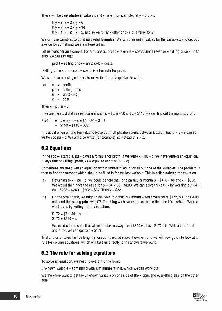
These will be true whatever values x and y have. For example, let y = 0.5 x
If y = 3, x = 2 y = 6 If y = 7, x = 2 y = 14 If y = 1, x = 2 y = 2, and so on for any other choice of a value for y.
We can use variables to build up useful formulae. We can then put in values for the variables, and get out a value for something we are interested in.
Let us consider an example. For a business, profit = revenue – costs. Since revenue = selling price units sold, we can say that
profit = selling price units sold – costs.
'Selling price units sold – costs' is a formula for profit.
We can then use single letters to make the formula quicker to write.
Let x = profit p = selling price u = units sold c = cost
Then x = p u – c.
If we are then told that in a particular month, p = $5, u = 30 and c = $118, we can find out the month's profit.
Profit = x = p u – c = $5 30 – $118 = $150 – $118 = $32.
It is usual when writing formulae to leave out multiplication signs between letters. Thus p u – c can be written as pu – c. We will also write (for example) 2x instead of 2 x.
6.2 Equations In the above example, pu – c was a formula for profit. If we write x = pu – c, we have written an equation. It says that one thing (profit, x) is equal to another (pu – c).
Sometimes, we are given an equation with numbers filled in for all but one of the variables. The problem is then to find the number which should be filled in for the last variable. This is called solving the equation.
(a) Returning to x = pu – c, we could be told that for a particular month p = $4, u = 60 and c = $208. We would then have the equation x = $4 60 – $208. We can solve this easily by working out $4 60 – $208 = $240 – $208 = $32. Thus x = $32.
(b) On the other hand, we might have been told that in a month when profits were $172, 50 units were sold and the selling price was $7. The thing we have not been told is the month's costs, c. We can work out c by writing out the equation.
$172 = $7 50 – c $172 = $350 – c
We need c to be such that when it is taken away from $350 we have $172 left. With a bit of trial and error, we can get to c = $178.
Trial and error takes far too long in more complicated cases, however, and we will now go on to look at a rule for solving equations, which will take us directly to the answers we want.
6.3 The rule for solving equationsTo solve an equation, we need to get it into the form:
Unknown variable = something with just numbers in it, which we can work out.
We therefore want to get the unknown variable on one side of the = sign, and everything else on the other side.

Basic maths 11
The rule is that you can do what you like to one side of an equation, so long as you do the same thing to the other side straightaway. The two sides are equal, and they will stay equal so long as you treat them in the same way.
For example, you can do any of the following.
Add 37 to both sides. Subtract 3x from both sides. Multiply both sides by –4.329. Divide both sides by (x + 2). Take the reciprocal of both sides. Square both sides. Take the cube root of both sides.
We can do any of these things to an equation either before or after filling in numbers for the variables for which we have values.
(a) In Paragraph 6.2, we had
$172 = $350 – c.
We can then get
$172 + c = $350 (add c to each side) c = $350 – $172 (subtract $172 from each side) c = $178 (work out the right hand side).
(b) 450 = 3x + 72 (initial equation: x unknown) 450 – 72 = 3x (subtract 72 from each side)
3
72450= x (divide each side by 3)
126 = x (work out the left hand side).
(c) 3y + 2 = 5y – 7 (initial equation: y unknown) 3y + 9 = 5y (add 7 to each side) 9 = 2y (subtract 3y from each side) 4.5 = y (divide each side by 2).
(d)x2
xx3 2
= 7 (initial equation: x unknown)
x4xx3 2
= 49 (square each side)
4)1x3( = 49 (cancel x in the numerator and the denominator of the left hand side: this does not affect the value of the left hand side, so we do not need to change the right hand side)
3x + 1 = 196 (multiply each side by 4)
3x = 195 (subtract 1 from each side)
x = 65 (divide each side by 3).
(e) Our example in Paragraph 6.1 was x = pu – c. We could change this, so as to give a formula for p.
x = pu – c
x + c = pu (add c to each side)
ucx
= p (divide each side by u)
p =u
cx(swap the sides for ease of reading).
Given values for x, c and u we can now find p. We have re-arranged the equation to give p in termsof x, c and u.

12 Basic maths
(f) Given that y = 7x3 , we can get an equation giving x in terms of y.
y = 7x3
y2 = 3x + 7 (square each side)
y2 – 7 = 3x (subtract 7 from each side)
x = 3
7y 2
(divide each side by 3, and swap the sides for ease of reading).
(g) Given that 7 + g = h3
5, we can get an equation giving h in terms of g.
7 + g = h3
5
5h3
g71
(take the reciprocal of each side)
h3g7
5(multiply each side by 5)
hg)7(3
5(divide each side by 3)
2g)7(925
h (square each side, and swap the sides for ease of reading).
In equations, you may come across expressions like 3(x + 4y – 2) (that is, 3 (x + 4y – 2)). These can be re-written in separate bits without the brackets, simply by multiplying the number outside the brackets by each item inside them. Thus 3(x + 4y – 2) = 3x + 12y – 6.
Question Equations
Find the value of x in each of the following equations.
(a) 47x + 256 = 52x (b) x4 + 32 = 40.6718
(c)2x7.2
5
4x3
1
(d) x3 = 4.913 (e) 34x – 7.6 = (17x – 3.8) (x + 12.5)
Answer(a) 47x + 256 = 52x
256 = 5x (subtract 47x from each side) 51.2 = x (divide each side by 5).
(b) x4 + 32 = 40.6718 x4 = 8.6718 (subtract 32 from each side) x = 2.16795 (divide each side by 4)
x = 4.7 (square each side).
(c)4x3
1 =
2x7.25
3x + 4 = 5
2x7.2 (take the reciprocal of each side)
15x + 20 = 2.7x – 2 (multiply each side by 5) 12.3x = –22 (subtract 20 and subtract 2.7x from each side) x = –1.789 (divide each side by 12.3).

Basic maths 13
(d) x3 = 4.913 x = 1.7 (take the cube root of each side).
(e) 34x – 7.6 = (17x – 3.8) (x + 12.5)
This one is easy if you realise that 17 2 = 34 and 3.8 2 = 7.6, so
2 (17x – 3.8) = 34x – 7.6.
We can then divide each side by 17x – 3.8 to get
2 = x + 12.5 –10.5 = x (subtract 12.5 from each side).
Question Re-arrange
(a) Re-arrange x = (3y – 20)2 to get an expression for y in terms of x. (b) Re-arrange 2(y – 4) – 4(x2 + 3) = 0 to get an expression for x in terms of y.
Answer(a) x = (3y – 20)2
x = 3y – 20 (take the square root of each side)
20 + x = 3y (add 20 to each side)
y =3
x20 (divide each side by 3, and swap the sides for ease of reading).
(b) 2(y – 4) – 4(x2 + 3) = 0 2(y – 4) = 4 (x2 + 3) (add 4(x2 + 3) to each side)0.5(y – 4) = x2 + 3 (divide each side by 4) 0.5(y – 4) – 3 = x2 (subtract 3 from each side)
x = 3)4(y5.0 (take the square root of each side, and swap the sides for ease of reading)
x = 5y5.0 (simplify 0.5(y-4) – 3: this is an optional last step).
7 Linear equations 7.1 Introduction A linear equation has the general form y = a + bx
where y is the dependent variable whose value depends upon the value of x; x is the independent variable whose value helps to determine the corresponding value of y; a is a constant, that is, a fixed amount; b is also a constant, being the coefficient of x (that is, the number by which the value of x
should be multiplied to derive the value of y).
Let us establish some basic linear equations. Suppose that it takes Joe Bloggs 15 minutes to walk one mile. How long does it take Joe to walk two miles? Obviously it takes him 30 minutes. How did you calculate the time? You probably thought that if the distance is doubled then the time must be doubled. How do you explain (in words) the relationships between the distance walked and the time taken? One explanation would be that every mile walked takes 15 minutes.
That is an explanation in words. Can you explain the relationship with an equation?
14 Basic maths
First you must decide which is the dependent variable and which is the independent variable. In other words, does the time taken depend on the number of miles walked or does the number of miles walked depend on the time it takes to walk a mile? Obviously the time depends on the distance. We can therefore let y be the dependent variable (time taken in minutes) and x be the independent variable (distance walked in miles).
We now need to determine the constants a and b. There is no fixed amount so a = 0. To ascertain b, we need to establish the number of times by which the value of x should be multiplied to derive the value of y. Obviously y = 15x where y is in minutes. If y were in hours then y = x/4.
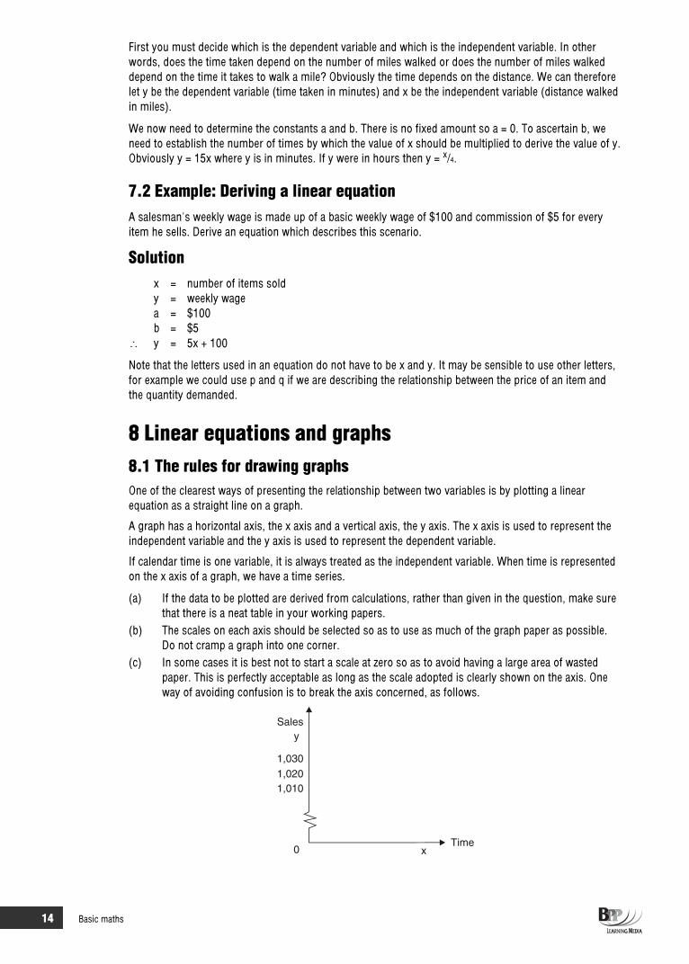
7.2 Example: Deriving a linear equation A salesman's weekly wage is made up of a basic weekly wage of $100 and commission of $5 for every item he sells. Derive an equation which describes this scenario.
Solution x = number of items sold y = weekly wage a = $100 b = $5
y = 5x + 100
Note that the letters used in an equation do not have to be x and y. It may be sensible to use other letters, for example we could use p and q if we are describing the relationship between the price of an item and the quantity demanded.
8 Linear equations and graphs 8.1 The rules for drawing graphs One of the clearest ways of presenting the relationship between two variables is by plotting a linear equation as a straight line on a graph.
A graph has a horizontal axis, the x axis and a vertical axis, the y axis. The x axis is used to represent the independent variable and the y axis is used to represent the dependent variable.
If calendar time is one variable, it is always treated as the independent variable. When time is represented on the x axis of a graph, we have a time series.
(a) If the data to be plotted are derived from calculations, rather than given in the question, make sure that there is a neat table in your working papers.
(b) The scales on each axis should be selected so as to use as much of the graph paper as possible. Do not cramp a graph into one corner.
(c) In some cases it is best not to start a scale at zero so as to avoid having a large area of wasted paper. This is perfectly acceptable as long as the scale adopted is clearly shown on the axis. One way of avoiding confusion is to break the axis concerned, as follows.
0Time
Salesy
1,0301,0201,010
x

Basic maths 15
(d) The scales on the x axis and the y axis should be marked. For example, if the y axis relates to amounts of money, the axis should be marked at every $1, or $100 or $1,000 interval or at whatever other interval is appropriate. The axes must be marked with values to give the reader an idea of how big the values on the graph are.
(e) A graph should not be overcrowded with too many lines. Graphs should always give a clear, neat impression.
(f) A graph must always be given a title, and where appropriate, a reference should be made to the source of data.
8.2 Example: Drawing graphs Plot the graphs for the following relationships.
(a) y = 4x + 5 (b) y = 10 – x
In each case consider the range of values from x = 0 to x = 10
SolutionThe first step is to draw up a table for each equation. Although the problem mentions x = 0 to x = 10, it is not necessary to calculate values of y for x = 1, 2, 3 etc. A graph of a linear equation can actually be drawn from just two (x, y) values but it is always best to calculate a number of values in case you make an arithmetical error. We have calculated six values. You could settle for three or four.
(a) (b) x y x y 0 5 0 10 2 13 2 8 4 21 4 6 6 29 6 4 8 37 8 2
10 45 10 0
(a)
0
5
15
25
35
45
2 4 6 8 10
y
x
Graph of y = 4x +5
16 Basic maths
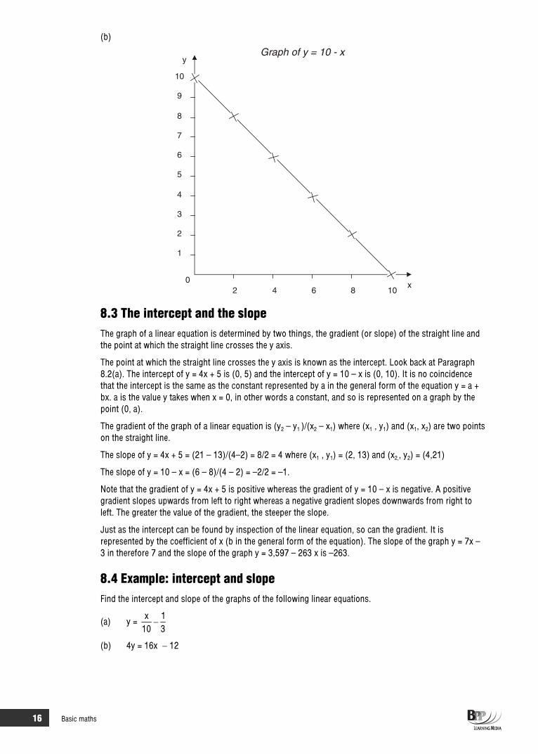
(b)
1
02 4 6 8 10
x
10
y
2
3
4
5
6
7
8
9
Graph of y = 10 - x
8.3 The intercept and the slope The graph of a linear equation is determined by two things, the gradient (or slope) of the straight line and the point at which the straight line crosses the y axis.
The point at which the straight line crosses the y axis is known as the intercept. Look back at Paragraph 8.2(a). The intercept of y = 4x + 5 is (0, 5) and the intercept of y = 10 – x is (0, 10). It is no coincidence that the intercept is the same as the constant represented by a in the general form of the equation y = a + bx. a is the value y takes when x = 0, in other words a constant, and so is represented on a graph by the point (0, a).
The gradient of the graph of a linear equation is (y2 – y1 )/(x2 – x1) where (x1 , y1) and (x1, x2) are two points on the straight line.
The slope of y = 4x + 5 = (21 – 13)/(4–2) = 8/2 = 4 where (x1 , y1) = (2, 13) and (x2,, y2) = (4,21)
The slope of y = 10 – x = (6 – 8)/(4 – 2) = –2/2 = –1.
Note that the gradient of y = 4x + 5 is positive whereas the gradient of y = 10 – x is negative. A positive gradient slopes upwards from left to right whereas a negative gradient slopes downwards from right to left. The greater the value of the gradient, the steeper the slope.
Just as the intercept can be found by inspection of the linear equation, so can the gradient. It is represented by the coefficient of x (b in the general form of the equation). The slope of the graph y = 7x – 3 in therefore 7 and the slope of the graph y = 3,597 – 263 x is –263.
8.4 Example: intercept and slope Find the intercept and slope of the graphs of the following linear equations.
(a) y = 31
10x
(b) 4y = 16x 12

Basic maths 17
Solution
(a) Intercept = a = 31
ie (0, 31
)
Slope = b = 101
(b) 4y = 16x 12
Equation must be form y = a + bx
y = 4
164
12 x = –3 + 4x
Intercept = a = 3 ie (0, 3)
Slope = 4
9 Simultaneous linear equations 9.1 Introduction Simultaneous equations are two or more equations which are satisfied by the same variable values. For example, we might have the following two linear equations.
y = 3x + 16 2y = x + 72
There are two unknown values, x and y, and there are two different equations which both involve x and y. There are as many equations as there are unknowns and so we can find the values of x and y.
9.2 Graphical solution One way of finding a solution is by a graph. If both equations are satisfied together, the values of x and y must be those where the straight line graphs of the two equations intersect.
10
20
30
40
02 4 6 8 10 12
y
x
y = 3x + 16
2y = x +72
Since both equations are satisfied, the values of x and y must lie on both the lines. Since this happens only once, at the intersection of the lines, the value of x must be 8, and of y 40.
9.3 Algebraic solution A more common method of solving simultaneous equations is by algebra.
(a) Returning to the original equations, we have:
y = 3x + 16 (1) 2y = x + 72 (2)

18 Basic maths
(b) Rearranging these, we have:
y – 3x = 16 (3) 2y – x = 72 (4)
(c) If we now multiply equation (4) by 3, so that the coefficient for x becomes the same as in equation (3) we get:
6y – 3x = 216 (5)y – 3x = 16 (3)
(d) Subtracting (3) from (5) means that we lose x and we get:
5y = 200 y = 40
(e) Substituting 40 for y in any equation, we can derive a value for x. Thus substituting in equation (4) we get:
2(40) – x = 72 80 – 72 = x 8 = x
(f) The solution is y = 40, x = 8.
9.4 Example: Simultaneous equations Solve the following simultaneous equations using algebra.
5x + 2y = 34 x + 3y = 25
Solution 5x + 2y = 34 (1) x + 3y = 25 (2) 5x + 15y = 125 (3) 5 (2) 13y = 91 (4) (3) – (1)
y = 7 x + 21 = 25 Substitute into (2)
x = 25 – 21 x = 4
The solution is x = 4, y = 7.
Question Simultaneous equations
Solve the following simultaneous equations to derive values for x and y.
4x + 3y = 23 (1) 5x – 4y = –10 (2)
Answer(a) If we multiply equation (1) by 4 and equation (2) by 3, we will obtain coefficients of +12 and –12
for y in our two products.
16x + 12y = 92 (3) 15x – 12y = –30 (4)

Basic maths 19
(b) Add (3) and (4).
31x = 62 x = 2
(c) Substitute x = 2 into (1)
4(2) + 3y = 23 3y = 23 – 8 = 15 y = 5
(d) The solution is x = 2, y = 5.
10 Summary of chapter Now that you have completed this introductory chapter, you should hopefully feel more confident about dealing with various mathematical techniques. Continue to refer to this chapter throughout your studies, as the techniques are used frequently for solving management accounting problems.

20 Basic maths
21
The nature and purpose of cost and management accounting
P
A
R
T
A

22

23
Information for management
IntroductionThis and the following two chapters provide an introduction to ManagementAccounting. This chapter looks at information and introduces cost accounting.Chapters 2 and 3 provide basic information on how costs are classified and how they behave.
Topic list Syllabus reference
1 Information A1 (a)
2 Planning, control and decision-making A1 (b)
3 Financial accounting and cost and management accounting
A2 (a)
4 Presentation of information to management A1 (a)
24 1: Information for management Part A The nature and purpose of cost and management accounting
Study guide Intellectual level
A1 Accounting for management
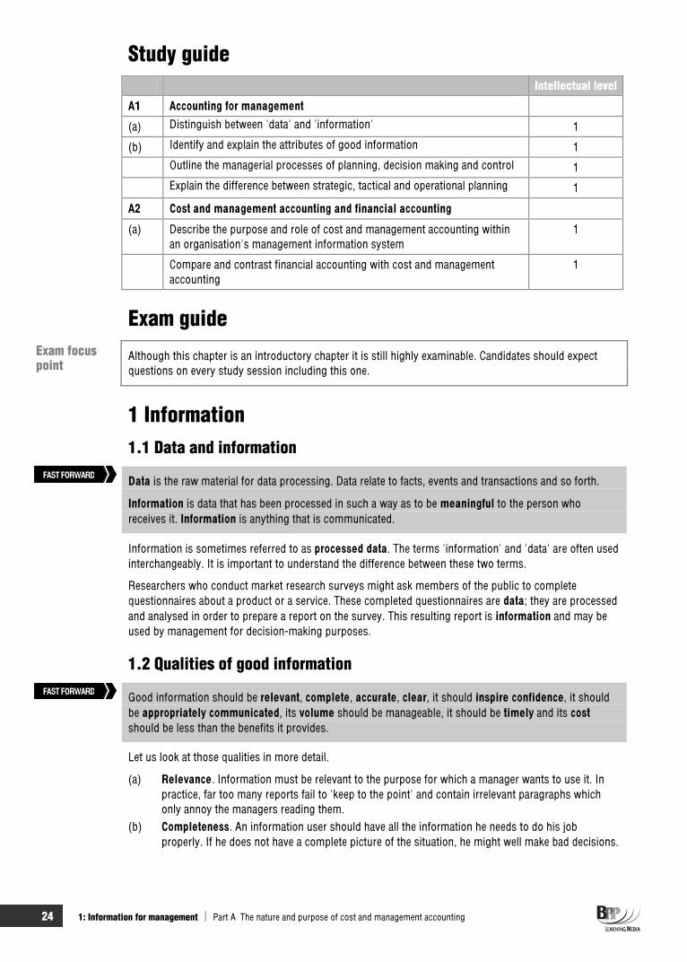
(a) Distinguish between 'data' and 'information' 1
(b) Identify and explain the attributes of good information 1
Outline the managerial processes of planning, decision making and control 1
Explain the difference between strategic, tactical and operational planning 1
A2 Cost and management accounting and financial accounting
(a) Describe the purpose and role of cost and management accounting within an organisation's management information system
1
Compare and contrast financial accounting with cost and management accounting
1
Exam guide
Although this chapter is an introductory chapter it is still highly examinable. Candidates should expect questions on every study session including this one.
1 Information 1.1 Data and information
Data is the raw material for data processing. Data relate to facts, events and transactions and so forth.
Information is data that has been processed in such a way as to be meaningful to the person who receives it. Information is anything that is communicated.
Information is sometimes referred to as processed data. The terms 'information' and 'data' are often used interchangeably. It is important to understand the difference between these two terms.
Researchers who conduct market research surveys might ask members of the public to complete questionnaires about a product or a service. These completed questionnaires are data; they are processed and analysed in order to prepare a report on the survey. This resulting report is information and may be used by management for decision-making purposes.
1.2 Qualities of good information
Good information should be relevant, complete, accurate, clear, it should inspire confidence, it should be appropriately communicated, its volume should be manageable, it should be timely and its costshould be less than the benefits it provides.
Let us look at those qualities in more detail.
(a) Relevance. Information must be relevant to the purpose for which a manager wants to use it. In practice, far too many reports fail to 'keep to the point' and contain irrelevant paragraphs which only annoy the managers reading them.
(b) Completeness. An information user should have all the information he needs to do his job properly. If he does not have a complete picture of the situation, he might well make bad decisions.
FAST FORWARD
FAST FORWARD
Exam focus point

Part A The nature and purpose of cost and management accounting 1: Information for management 25
(c) Accuracy. Information should obviously be accurate because using incorrect information could have serious and damaging consequences. However, information should only be accurate enough for its purpose and there is no need to go into unnecessary detail for pointless accuracy.
(d) Clarity. Information must be clear to the user. If the user does not understand it properly he cannot use it properly. Lack of clarity is one of the causes of a breakdown in communication. It is therefore important to choose the most appropriate presentation medium or channel of communication.
(e) Confidence. Information must be trusted by the managers who are expected to use it. However not all information is certain. Some information has to be certain, especially operating information, for example, related to a production process. Strategic information, especially relating to the environment, is uncertain. However, if the assumptions underlying it are clearly stated, this might enhance the confidence with which the information is perceived.
(f) Communication. Within any organisation, individuals are given the authority to do certain tasks, and they must be given the information they need to do them. An office manager might be made responsible for controlling expenditures in his office, and given a budget expenditure limit for the year. As the year progresses, he might try to keep expenditure in check but unless he is told throughout the year what is his current total expenditure to date, he will find it difficult to judge whether he is keeping within budget or not.
(g) Volume. There are physical and mental limitations to what a person can read, absorb and understand properly before taking action. An enormous mountain of information, even if it is all relevant, cannot be handled. Reports to management must therefore be clear and concise and in many systems, control action works basically on the 'exception' principle.
(h) Timing. Information which is not available until after a decision is made will be useful only for comparisons and longer-term control, and may serve no purpose even then. Information prepared too frequently can be a serious disadvantage. If, for example, a decision is taken at a monthly meeting about a certain aspect of a company's operations, information to make the decision is only required once a month, and weekly reports would be a time-consuming waste of effort.
(i) Channel of communication. There are occasions when using one particular method of communication will be better than others. For example, job vacancies should be announced in a medium where they will be brought to the attention of the people most likely to be interested. The channel of communication might be the company's in-house journal, a national or local newspaper, a professional magazine, a job centre or school careers office. Some internal memoranda may be better sent by 'electronic mail'. Some information is best communicated informally by telephone or word-of-mouth, whereas other information ought to be formally communicated in writing or figures.
(j) Cost. Information should have some value, otherwise it would not be worth the cost of collecting and filing it. The benefits obtainable from the information must also exceed the costs of acquiring it, and whenever management is trying to decide whether or not to produce information for a particular purpose (for example whether to computerise an operation or to build a financial planning model) a cost/benefit study ought to be made.
Question Value of information
The value of information lies in the action taken as a result of receiving it. What questions might you ask in order to make an assessment of the value of information?
Answer(a) What information is provided? (b) What is it used for? (c) Who uses it? (d) How often is it used? (e) Does the frequency with which it is used coincide with the frequency with which it is provided?

26 1: Information for management Part A The nature and purpose of cost and management accounting
(f) What is achieved by using it? (g) What other relevant information is available which could be used instead?
An assessment of the value of information can be derived in this way, and the cost of obtaining it should then be compared against this value. On the basis of this comparison, it can be decided whether certain items of information are worth having. It should be remembered that there may also be intangible benefits which may be harder to quantify.
1.3 Why is information important? Consider the following problems and what management needs to solve these problems.
(a) A company wishes to launch a new product. The company's pricing policy is to charge cost plus 20%. What should the price of the product be?
(b) An organisation's widget-making machine has a fault. The organisation has to decide whether to repair the machine, buy a new machine or hire a machine. What does the organisation do if its aim is to control costs?
(c) A firm is considering offering a discount of 2% to those customers who pay an invoice within seven days of the invoice date and a discount of 1% to those customers who pay an invoice within eight to fourteen days of the invoice date. How much will this discount offer cost the firm?
In solving these and a wide variety of other problems, management need information.
(a) In problem (a) above, management would need information about the cost of the new product.(b) Faced with problem (b), management would need information on the cost of repairing, buying and
hiring the machine.(c) To calculate the cost of the discount offer described in (c), information would be required about
current sales settlement patterns and expected changes to the pattern if discounts were offered.
The successful management of any organisation depends on information: non-profit making organisations such as charities, clubs and local authorities need information for decision making and for reporting the results of their activities just as multi-nationals do. For example a tennis club needs to know the cost of undertaking its various activities so that it can determine the amount of annual subscription it should charge its members.
1.4 What type of information is needed? Most organisations require the following types of information.
Financial Non-financial A combination of financial and non-financial information
1.4.1 Example: Financial and non-financial information
Suppose that the management of ABC Co have decided to provide a canteen for their employees.
(a) The financial information required by management might include canteen staff costs, costs of subsidising meals, capital costs, costs of heat and light and so on.
(b) The non-financial information might include management comment on the effect on employee morale of the provision of canteen facilities, details of the number of meals served each day, meter readings for gas and electricity and attendance records for canteen employees.
ABC Co could now combine financial and non-financial information to calculate the average cost to the company of each meal served, thereby enabling them to predict total costs depending on the number of employees in the work force.
Part A The nature and purpose of cost and management accounting 1: Information for management 27
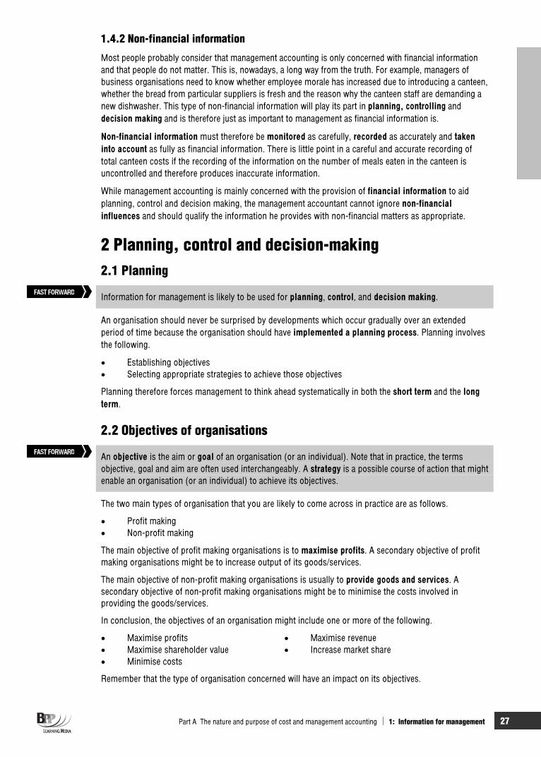
1.4.2 Non-financial information
Most people probably consider that management accounting is only concerned with financial information and that people do not matter. This is, nowadays, a long way from the truth. For example, managers of business organisations need to know whether employee morale has increased due to introducing a canteen, whether the bread from particular suppliers is fresh and the reason why the canteen staff are demanding a new dishwasher. This type of non-financial information will play its part in planning, controlling and decision making and is therefore just as important to management as financial information is.
Non-financial information must therefore be monitored as carefully, recorded as accurately and takeninto account as fully as financial information. There is little point in a careful and accurate recording of total canteen costs if the recording of the information on the number of meals eaten in the canteen is uncontrolled and therefore produces inaccurate information.
While management accounting is mainly concerned with the provision of financial information to aid planning, control and decision making, the management accountant cannot ignore non-financialinfluences and should qualify the information he provides with non-financial matters as appropriate.
2 Planning, control and decision-making 2.1 Planning
Information for management is likely to be used for planning, control, and decision making.
An organisation should never be surprised by developments which occur gradually over an extended period of time because the organisation should have implemented a planning process. Planning involves the following.
Establishing objectives Selecting appropriate strategies to achieve those objectives
Planning therefore forces management to think ahead systematically in both the short term and the longterm.
2.2 Objectives of organisations
An objective is the aim or goal of an organisation (or an individual). Note that in practice, the terms objective, goal and aim are often used interchangeably. A strategy is a possible course of action that might enable an organisation (or an individual) to achieve its objectives.
The two main types of organisation that you are likely to come across in practice are as follows.
Profit making Non-profit making
The main objective of profit making organisations is to maximise profits. A secondary objective of profit making organisations might be to increase output of its goods/services.
The main objective of non-profit making organisations is usually to provide goods and services. A secondary objective of non-profit making organisations might be to minimise the costs involved in providing the goods/services.
In conclusion, the objectives of an organisation might include one or more of the following.
Maximise profits Maximise revenue Maximise shareholder value Increase market share Minimise costs
Remember that the type of organisation concerned will have an impact on its objectives.
FAST FORWARD
FAST FORWARD

28 1: Information for management Part A The nature and purpose of cost and management accounting
2.3 Strategy and organisational structure There are two schools of thought on the link between strategy and organisational structure.
Structure follows strategy Strategy follows structure
Let's consider the first idea that structure follows strategy. What this means is that organisations develop strategies in order that they can cope with changes in the structure of an organisation. Or do they?
The second school of thought suggests that strategy follows structure. This side of the argument suggests that the strategy of an organisation is determined or influenced by the structure of the organisation. The structure of the organisation therefore limits the number of strategies available.
We could explore these ideas in much more detail, but for the purposes of your Management Accounting studies, you really just need to be aware that there is a link between strategy and the structure of an organisation.
2.4 Long-term strategic planning
Long-term planning, also known as corporate planning, involves selecting appropriate strategies so as to prepare a long-term plan to attain the objectives.
The time span covered by a long-term plan depends on the organisation, the industry in which it operates and the particular environment involved. Typical periods are 2, 5, 7 or 10 years although longer periods are frequently encountered.
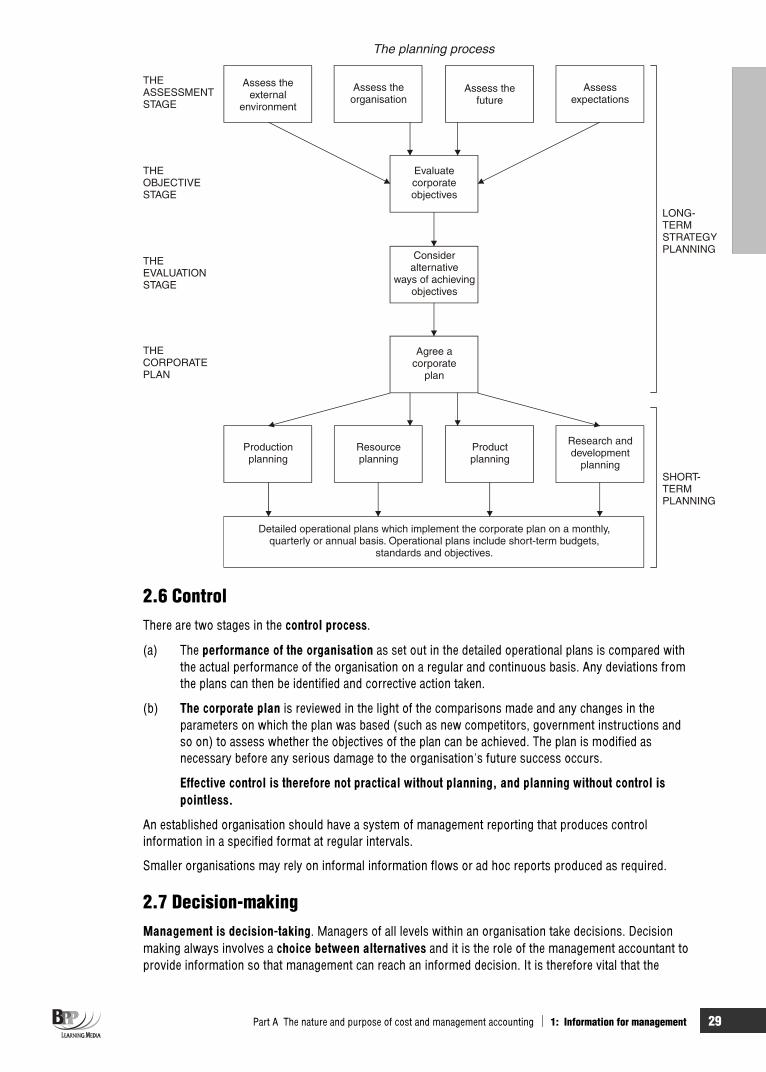
Long-term strategic planning is a detailed, lengthy process, essentially incorporating three stages and ending with a corporate plan. The diagram on the next page provides an overview of the process and shows the link between short-term and long-term planning.
2.5 Short-term tactical planning The long-term corporate plan serves as the long-term framework for the organisation as a whole but for operational purposes it is necessary to convert the corporate plan into a series of short-term plans,usually covering one year, which relate to sections, functions or departments. The annual process of short-term planning should be seen as stages in the progressive fulfilment of the corporate plan as each short-term plan steers the organisation towards its long-term objectives. It is therefore vital that, to obtain the maximum advantage from short-term planning, some sort of long-term plan exists.
Key term
Part A The nature and purpose of cost and management accounting 1: Information for management 29
2.6 Control There are two stages in the control process.
(a) The performance of the organisation as set out in the detailed operational plans is compared with the actual performance of the organisation on a regular and continuous basis. Any deviations from the plans can then be identified and corrective action taken.
(b) The corporate plan is reviewed in the light of the comparisons made and any changes in the parameters on which the plan was based (such as new competitors, government instructions and so on) to assess whether the objectives of the plan can be achieved. The plan is modified as necessary before any serious damage to the organisation's future success occurs.
Effective control is therefore not practical without planning, and planning without control is pointless.
An established organisation should have a system of management reporting that produces control information in a specified format at regular intervals.
Smaller organisations may rely on informal information flows or ad hoc reports produced as required.
2.7 Decision-making Management is decision-taking. Managers of all levels within an organisation take decisions. Decision making always involves a choice between alternatives and it is the role of the management accountant to provide information so that management can reach an informed decision. It is therefore vital that the

30 1: Information for management Part A The nature and purpose of cost and management accounting
management accountant understands the decision-making process so that he can supply the appropriate type of information.
2.7.1 Decision-making process
2.8 Anthony's view of management activity
Anthony divides management activities into strategic planning, management control and operationalcontrol.
R N Anthony, a leading writer on organisational control, has suggested that the activities of planning,control and decision making should not be separated since all managers make planning and control decisions. He has identified three types of management activity.
(a) Strategic planning: 'the process of deciding on objectives of the organisation, on changes in these objectives, on the resources used to attain these objectives, and on the policies that are to govern the acquisition, use and disposition of these resources'.
(b) Management control: 'the process by which managers assure that resources are obtained and used effectively and efficiently in the accomplishment of the organisation's objectives'.
(c) Operational control: 'the process of assuring that specific tasks are carried out effectively and efficiently'.
FAST FORWARD

Part A The nature and purpose of cost and management accounting 1: Information for management 31
2.8.1 Strategic planning
Strategic plans are those which set or change the objectives, or strategic targets of an organisation. They would include such matters as the selection of products and markets, the required levels of company profitability, the purchase and disposal of subsidiary companies or major fixed assets and so on.
2.8.2 Management control
Whilst strategic planning is concerned with setting objectives and strategic targets, management controlis concerned with decisions about the efficient and effective use of an organisation's resources to achieve these objectives or targets.
(a) Resources, often referred to as the '4 Ms' (men, materials, machines and money). (b) Efficiency in the use of resources means that optimum output is achieved from the input resources
used. It relates to the combinations of men, land and capital (for example how much production work should be automated) and to the productivity of labour, or material usage.
(c) Effectiveness in the use of resources means that the outputs obtained are in line with the intended objectives or targets.
2.8.3 Operational control
The third, and lowest tier, in Anthony's hierarchy of decision making, consists of operational control decisions. As we have seen, operational control is the task of ensuring that specific tasks are carried out effectively and efficiently. Just as 'management control' plans are set within the guidelines of strategic plans, so too are 'operational control' plans set within the guidelines of both strategic planning and management control. Consider the following.
(a) Senior management may decide that the company should increase sales by 5% per annum for at least five years – a strategic plan.
(b) The sales director and senior sales managers will make plans to increase sales by 5% in the next year, with some provisional planning for future years. This involves planning direct sales resources, advertising, sales promotion and so on. Sales quotas are assigned to each sales territory – a tactical plan (management control).
(c) The manager of a sales territory specifies the weekly sales targets for each sales representative. This is operational planning: individuals are given tasks which they are expected to achieve.
Although we have used an example of selling tasks to describe operational control, it is important to remember that this level of planning occurs in all aspects of an organisation's activities, even when the activities cannot be scheduled nor properly estimated because they are non-standard activities (such as repair work, answering customer complaints).
The scheduling of unexpected or 'ad hoc' work must be done at short notice, which is a feature of much operational planning. In the repairs department, for example, routine preventive maintenance can be scheduled, but breakdowns occur unexpectedly and repair work must be scheduled and controlled 'on the spot' by a repairs department supervisor.
2.9 Management control systems
A management control system is a system which measures and corrects the performance of activities of subordinates in order to make sure that the objectives of an organisation are being met and the plans devised to attain them are being carried out.
The management function of control is the measurement and correction of the activities of subordinates in order to make sure that the goals of the organisation, or planning targets are achieved.
The basic elements of a management control system are as follows.
Planning: deciding what to do and identifying the desired results Recording the plan which should incorporate standards of efficiency or targets
FAST FORWARD

32 1: Information for management Part A The nature and purpose of cost and management accounting
Carrying out the plan and measuring actual results achieved Comparing actual results against the plans Evaluating the comparison, and deciding whether further action is necessary
Where corrective action is necessary, this should be implemented
2.10 Types of information
Information within an organisation can be analysed into the three levels assumed in Anthony's hierarchy: strategic; tactical; and operational.
2.10.1 Strategic information
Strategic information is used by senior managers to plan the objectives of their organisation, and to assess whether the objectives are being met in practice. Such information includes overall profitability,the profitability of different segments of the business, capital equipment needs and so on.
Strategic information therefore has the following features.
It is derived from both internal and external sources. It is summarised at a high level. It is relevant to the long term. It deals with the whole organisation (although it might go into some detail). It is often prepared on an 'ad hoc' basis. It is both quantitative and qualitative (see below). It cannot provide complete certainty, given that the future cannot be predicted.
2.10.2 Tactical information
Tactical information is used by middle management to decide how the resources of the business should be employed, and to monitor how they are being and have been employed. Such information includes productivity measurements (output per man hour or per machine hour), budgetary control or varianceanalysis reports, and cash flow forecasts and so on.
Tactical information therefore has the following features.
It is primarily generated internally. It is summarised at a lower level. It is relevant to the short and medium term. It describes or analyses activities or departments. It is prepared routinely and regularly. It is based on quantitative measures.
2.10.3 Operational information
Operational information is used by 'front-line' managers such as foremen or head clerks to ensure that specific tasks are planned and carried out properly within a factory or office and so on. In the payroll office, for example, information at this level will relate to day-rate labour and will include the hours worked each week by each employee, his rate of pay per hour, details of his deductions, and for the purpose of wages analysis, details of the time each man spent on individual jobs during the week. In this example, the information is required weekly, but more urgent operational information, such as the amount of raw materials being input to a production process, may be required daily, hourly, or in the case of automated production, second by second.
Operational information has the following features.
It is derived almost entirely from internal sources. It is highly detailed, being the processing of raw data. It relates to the immediate term, and is prepared constantly, or very frequently. It is task-specific and largely quantitative.
FAST FORWARD

Part A The nature and purpose of cost and management accounting 1: Information for management 33
3 Financial accounting and cost and management accounting
3.1 Financial accounts and management accounts
Financial accounting systems ensure that the assets and liabilities of a business are properly accounted for, and provide information about profits and so on to shareholders and to other interested parties. Management accounting systems provide information specifically for the use of managers within an organisation.
Management information provides a common source from which is drawn information for two groups of people.
(a) Financial accounts are prepared for individuals external to an organisation: shareholders, customers, suppliers, tax authorities, employees.
(b) Management accounts are prepared for internal managers of an organisation.
The data used to prepare financial accounts and management accounts are the same. The differences between the financial accounts and the management accounts arise because the data is analysed differently.
3.2 Financial accounts versus management accounts
Financial accounts Management accounts
Financial accounts detail the performance of an organisation over a defined period and the state of affairs at the end of that period.
Management accounts are used to aid management record, plan and control the organisation's activities and to help the decision-making process.
Limited liability companies must, by law, prepare financial accounts.
There is no legal requirement to prepare management accounts.
The format of published financial accounts is determined by local law, by International Accounting Standards and International Financial Reporting Standards. In principle the accounts of different organisations can therefore be easily compared.
The format of management accounts is entirely at management discretion: no strict rules govern the way they are prepared or presented. Each organisation can devise its own management accounting system and format of reports.
Financial accounts concentrate on the business as a whole, aggregating revenues and costs from different operations, and are an end in themselves.
Management accounts can focus on specific areas of an organisation's activities. Information may be produced to aid a decision rather than to be an end product of a decision.
Most financial accounting information is of a monetary nature.
Management accounts incorporate non-monetary measures. Management may need to know, for example, tons of aluminium produced, monthly machine hours, or miles travelled by salesmen.
Financial accounts present an essentially historic picture of past operations.
Management accounts are both an historical record and a future planning tool.
FAST FORWARD

34 1: Information for management Part A The nature and purpose of cost and management accounting
Question Management accounts
Which of the following statements about management accounts is/are true?
(i) There is a legal requirement to prepare management accounts. (ii) The format of management accounts is largely determined by law. (iii) They serve as a future planning tool and are not used as a historical record.
A (i) and (ii) B (ii) and (iii) C (iii) only D None of the statements are correct.
AnswerD
Statement (i) is incorrect. Limited liability companies must, by law, prepare financial accounts.
The format of published financial accounts is determined by law. Statement (ii) is therefore incorrect.
Management accounts do serve as a future planning tool but they are also useful as a historical record of performance. Therefore all three statements are incorrect and D is the correct answer.
3.3 Cost accounts
Cost accounting and management accounting are terms which are often used interchangeably. It is notcorrect to do so. Cost accounting is part of management accounting. Cost accounting provides a bank of data for the management accountant to use.
Cost accounting is concerned with the following.
Preparing statements (eg budgets, costing) Cost data collection Applying costs to inventory, products and services
Management accounting is concerned with the following.
Using financial data and communicating it as information to users
3.3.1 Aims of cost accounts
(a) The cost of goods produced or services provided. (b) The cost of a department or work section. (c) What revenues have been. (d) The profitability of a product, a service, a department, or the organisation in total. (e) Selling prices with some regard for the costs of sale. (f) The value of inventories of goods (raw materials, work in progress, finished goods) that are still
held in store at the end of a period, thereby aiding the preparation of a balance sheet of the company's assets and liabilities.
(g) Future costs of goods and services (costing is an integral part of budgeting (planning) for the future).
(h) How actual costs compare with budgeted costs. (If an organisation plans for its revenues and costs to be a certain amount, but they actually turn out differently, the differences can be measured and reported. Management can use these reports as a guide to whether corrective action (or
FAST FORWARD

Part A The nature and purpose of cost and management accounting 1: Information for management 35
'control' action) is needed to sort out a problem revealed by these differences between budgeted and actual results. This system of control is often referred to as budgetary control.
(i) What information management needs in order to make sensible decisions about profits and costs.
It would be wrong to suppose that cost accounting systems are restricted to manufacturing operations, although they are probably more fully developed in this area of work. Service industries, governmentdepartments and welfare activities can all make use of cost accounting information. Within a manufacturing organisation, the cost accounting system should be applied not only to manufacturing but also to administration, selling and distribution, research and development and all other departments.
4 Presentation of information to management
One of the optional performance objectives in your PER is ‘Prepare financial information for management’.ACCA suggests that in order to perform effectively, one of the skills you require is the ability to summarise and present financial information in a appropriate format for management purposes. This section contains information that can easily be put into practice to help you develop this skill.
4.1 Reports
Data and information are usually presented to management in the form of a report. The main features of a report are: TITLE; TO; FROM; DATE; and SUBJECT.
In small organisations it is possible, however, that information will be communicated in a less formal manner than writing a report (orally or using informal reports/memos).
Throughout this Study Text, you will come across a number of techniques which allow financial information to be collected. Once it has been collected it is usually analysed and reported back to management in the form of a report.
4.2 Main features of a report TITLE
Most reports are usually given a heading to show that it is a report. WHO IS THE REPORT INTENDED FOR?
It is vital that the intended recipients of a report are clearly identified. For example, if you are writing a report for Joe Bloggs, it should be clearly stated at the head of the report.
WHO IS THE REPORT FROM?
If the recipients of the report have any comments or queries, it is important that they know who to contact.
DATE
We have already mentioned that information should be communicated at the most appropriate time. It is also important to show this timeliness by giving your report a date.
SUBJECT
What is the report about? Managers are likely to receive a great number of reports that they need to review. It is useful to know what a report is about before you read it!
APPENDIX
In general, information is summarised in a report and the more detailed calculations and data are included in an appendix at the end of the report.
FAST FORWARD

36 1: Information for management Part A The nature and purpose of cost and management accounting
Chapter roundup
Data is the raw material for data processing. Data relate to facts, events and transactions and so forth.
Information is data that has been processed in such a way as to be meaningful to the person who receives it. Information is anything that is communicated.
Good information should be relevant, complete, accurate, clear, it should inspire confidence, it should be appropriately communicated, its volume should be manageable, it should be timely and its costshould be less than the benefits it provides.
Information for management accounting is likely to be used for planning, control and decision making.
An objective is the aim or goal of an organisation (or an individual). Note that in practice, the terms objective, goal and aim are often used interchangeably. A strategy is a possible course of action that might enable an organisation (or an individual) to achieve its objectives.
Anthony divides management activities into strategic planning, management control and operationalcontrol.
A management control system is a system which measures and corrects the performance of activities of subordinates in order to make sure that the objectives of an organisation are being met and the plans devised to attain them are being carried out.
Information within an organisation can be analysed into the three levels assumed in Anthony's hierarchy: strategic; tactical; and operational.
Financial accounting systems ensure that the assets and liabilities of a business are properly accounted for, and provide information about profits and so on to shareholders and to other interested parties. Management accounting systems provide information specifically for the use of managers within the organisation.
Cost accounting and management accounting are terms which are often used interchangeably. It is not correct to do so. Cost accounting is part of management accounting. Cost accounting provides a bank of data for the management accountant to use.
Data and information are usually presented to management in the form of a report. The main features of a report are: TITLE; TO; FROM; DATE; and SUBJECT.

Part A The nature and purpose of cost and management accounting 1: Information for management 37
Quick quiz 1 Define the terms data and information.
2 The four main qualities of good information are: ………………………. ………………………. ………………………. ……………………….
3 In terms of management accounting, information is most likely to be used for:
(1) ………………………. (2) ………………………. (3) ………………………. .
4 A strategy is the aim or goal of an organisation.
True
False
5 Organisation Objective
Profit making Non-profit making
6 What are the three types of management activity identified by R N Anthony?
(1) ………………………. (2) ………………………. (3) ……………………….
7 A management control system is
A A possible course of action that might enable an organisation to achieve its objectives
B A collective term for the hardware and software used to drive a database system
C A set up that measures and corrects the performance of activities of subordinates in order to make sure that the objectives of an organisation are being met and their associated plans are being carried out
D A system that controls and maximises the profits of an organisation
8 List six differences between financial accounts and management accounts.
9 When preparing reports, what are the five key points to remember?
………………………. ………………………. ………………………. ………………………. ……………………….

38 1: Information for management Part A The nature and purpose of cost and management accounting
Answers to quick quiz 1 Data is the raw material for data processing. Information is data that has been processed in such a way as
to be meaningful to the person who receives it. Information is anything that is communicated.
2 Relevance Accuracy Completeness Clarity
3 (1) Planning (2) Control (3) Decision making
4 False. This is the definition of an objective. A strategy is a possible course of action that might enable an organisation to achieve its objectives.
5 Profit making = maximise profits Non-profit making = provide goods and services
6 (1) Strategic planning (2) Management control (3) Operational control
7 C
8 See Paragraph 3.2
9 Title Who is the report to Who is the report from Date Subject
Now try the question below from the Exam Question Bank
Now try the questions below from the Exam Question Bank
Number Level Marks Time
Q1 MCQ n/a n/a

39
Cost classification, behaviour and purpose
P
A
R
T
B

40
41
Cost classification
IntroductionThe classification of costs as either direct or indirect, for example, is essential in the costing method used by an organisation to determine the cost of a unit of product or service.
The fixed and variable cost classifications, on the other hand, are important in absorption and marginal costing, cost behaviour and cost-volume-profitanalysis. You will meet all of these topics as we progress through the Study Text.
This chapter therefore acts as a foundation stone for a number of other chapters in the text and hence an understanding of the concepts covered in it is vital before you move on.
Topic list Syllabus reference
1 Total product/service costs B1 (a)
2 Direct costs and indirect costs B2 (a)
3 Functional costs B1 (a)
4 Fixed costs and variable costs B1 (d)
5 Production and non-production costs B1 (a)
6 Other cost classifications B1 (c)
7 Cost units, cost objects and responsibility centres A1 (a)

42 2: Cost classification Part B Cost classification, behaviour and purpose
Study guide Intellectual level
A1 Accounting for Management
(a) Distinguish between cost, profit, investment and revenue centres 1
(b) Describe the differing needs for information of cost, profit, investment and revenue centre managers
1
B1 Production and non-production costs
(a) Explain and illustrate production and non-production costs 1
(b) Describe the different elements of production cost – material, labour and overheads
1
(c) Describe the different elements of non-production cost – administrative, selling, distribution and finance
1
(d) Explain the importance of the distinction between production and non-production costs when valuing output and inventories
1
B2 Direct and indirect costs
(a) Distinguish between direct and indirect costs in manufacturing and non-manufacturing organisations
1
(b) Identify examples of direct and indirect costs in manufacturing and non-manufacturing organisations
1
(c) Explain and illustrate the concepts of cost objects, cost units and cost centres
1
Exam guide Cost classification is one of the key areas of the syllabus and you can therefore expect to see it in the exam that you will be facing.
1 Total product/service costs The total cost of making a product or providing a service consists of the following.
(a) Cost of materials
(b) Cost of the wages and salaries (labour costs)
(c) Cost of other expenses
(i) Rent and rates (ii) Electricity and gas bills (iii) Depreciation
2 Direct costs and indirect costs 2.1 Materials, labour and expenses
A direct cost is a cost that can be traced in full to the product, service, or department that is being costed. An indirect cost (or overhead) is a cost that is incurred in the course of making a product, providing a service or running a department, but which cannot be traced directly and in full to the product, service or department.
Materials, labour costs and other expenses can be classified as either direct costs or indirect costs.
FAST FORWARD

Part B Cost classification, behaviour and purpose 2: Cost classification 43
(a) Direct material costs are the costs of materials that are known to have been used in making and selling a product (or even providing a service).
(b) Direct labour costs are the specific costs of the workforce used to make a product or provide a service. Direct labour costs are established by measuring the time taken for a job, or the time taken in 'direct production work'.
(c) Other direct expenses are those expenses that have been incurred in full as a direct consequence of making a product, or providing a service, or running a department.
Examples of indirect costs include supervisors' wages, cleaning materials and buildings insurance.
2.2 Analysis of total cost Materials = Direct materials + Indirect materials
+ + +Labour = Direct labour + Indirect labour
+ + +Expenses = Direct expenses + Indirect expensesTotal cost = Direct cost + Overhead
2.3 Direct material
Direct material is all material becoming part of the product (unless used in negligible amounts and/or having negligible cost).
Direct material costs are charged to the product as part of the prime cost. Examples of direct material are as follows.
(a) Component parts, specially purchased for a particular job, order or process. (b) Part-finished work which is transferred from department 1 to department 2 becomes finished work
of department 1 and a direct material cost in department 2. (c) Primary packing materials like cartons and boxes.
2.4 Direct labour
Direct wages are all wages paid for labour (either as basic hours or as overtime) expended on work on the product itself.
Direct wages costs are charged to the product as part of the prime cost.
Examples of groups of labour receiving payment as direct wages are as follows.
(a) Workers engaged in altering the condition or composition of the product. (b) Inspectors, analysts and testers specifically required for such production. (c) Foremen, shop clerks and anyone else whose wages are specifically identified.
Two trends may be identified in direct labour costs.
The ratio of direct labour costs to total product cost is falling as the use of machinery increases, and hence depreciation charges increase.
Skilled labour costs and sub-contractors' costs are increasing as direct labour costs decrease.
Question Labour costs
Classify the following labour costs as either direct or indirect.
(a) The basic pay of direct workers (cash paid, tax and other deductions) (b) The basic pay of indirect workers (c) Overtime premium
Key term
Key term

44 2: Cost classification Part B Cost classification, behaviour and purpose
(d) Bonus payments (e) Social insurance contributions (f) Idle time of direct workers (g) Work on installation of equipment
Answer(a) The basic pay of direct workers is a direct cost to the unit, job or process.
(b) The basic pay of indirect workers is an indirect cost, unless a customer asks for an order to be carried out which involves the dedicated use of indirect workers' time, when the cost of this time would be a direct labour cost of the order.
(c) Overtime premium paid to both direct and indirect workers is an indirect cost, except in two particular circumstances.
(i) If overtime is worked at the specific request of a customer to get his order completed, the overtime premium paid is a direct cost of the order.
(ii) If overtime is worked regularly by a production department in the normal course of operations, the overtime premium paid to direct workers could be incorporated into the (average) direct labour hourly rate.
(d) Bonus payments are generally an indirect cost.
(e) Employer's National Insurance contributions (which are added to employees' total pay as a wages cost) are normally treated as an indirect labour cost.
(f) Idle time is an overhead cost, that is an indirect labour cost.
(g) The cost of work on capital equipment is incorporated into the capital cost of the equipment.
2.5 Direct expenses
Direct expenses are any expenses which are incurred on a specific product other than direct material cost and direct wages
Direct expenses are charged to the product as part of the prime cost. Examples of direct expenses are as follows.
The hire of tools or equipment for a particular job Maintenance costs of tools, fixtures and so on
Direct expenses are also referred to as chargeable expenses.
2.6 Production overhead
Production (or factory) overhead includes all indirect material costs, indirect wages and indirect expenses incurred in the factory from receipt of the order until its completion.
Production overhead includes the following.
(a) Indirect materials which cannot be traced in the finished product.
Consumable stores, eg material used in negligible amounts
(b) Indirect wages, meaning all wages not charged directly to a product.
Wages of non-productive personnel in the production department, eg foremen
(c) Indirect expenses (other than material and labour) not charged directly to production.
(i) Rent, rates and insurance of a factory (ii) Depreciation, fuel, power, maintenance of plant, machinery and buildings
Key term
Key term

Part B Cost classification, behaviour and purpose 2: Cost classification 45
2.7 Administration overhead
Administration overhead is all indirect material costs, wages and expenses incurred in the direction, control and administration of an undertaking.
Examples of administration overhead are as follows.
Depreciation of office buildings and equipment. Office salaries, including salaries of directors, secretaries and accountants.
Rent, rates, insurance, lighting, cleaning, telephone charges and so on.
2.8 Selling overhead
Selling overhead is all indirect materials costs, wages and expenses incurred in promoting sales and retaining customers.
Examples of selling overhead are as follows.
Printing and stationery, such as catalogues and price lists. Salaries and commission of salesmen, representatives and sales department staff. Advertising and sales promotion, market research.
Rent, rates and insurance of sales offices and showrooms, bad debts and so on.
2.9 Distribution overhead
Distribution overhead is all indirect material costs, wages and expenses incurred in making the packed product ready for despatch and delivering it to the customer.
Examples of distribution overhead are as follows.
Cost of packing cases. Wages of packers, drivers and despatch clerks. Insurance charges, rent, rates, depreciation of warehouses and so on.
Question Direct labour cost
A direct labour employee's wage in week 5 consists of the following.
$(a) Basic pay for normal hours worked, 36 hours at $4 per hour = 144
(b) Pay at the basic rate for overtime, 6 hours at $4 per hour = 24
(c) Overtime shift premium, with overtime paid at time-and-a-quarter ¼ 6 hours $4 per hour = 6
(d) A bonus payment under a group bonus (or 'incentive') scheme – bonus for the month = 30Total gross wages in week 5 for 42 hours of work 204
What is the direct labour cost for this employee in week 5?
A $144 B $168 C $198 D $204
AnswerLet's start by considering a general approach to answering multiple choice questions (MCQs). In a numerical question like this, the best way to begin is to ignore the available options and work out your own answer from the available data. If your solution corresponds to one of the four options then mark this
Key term
Key term
Key term
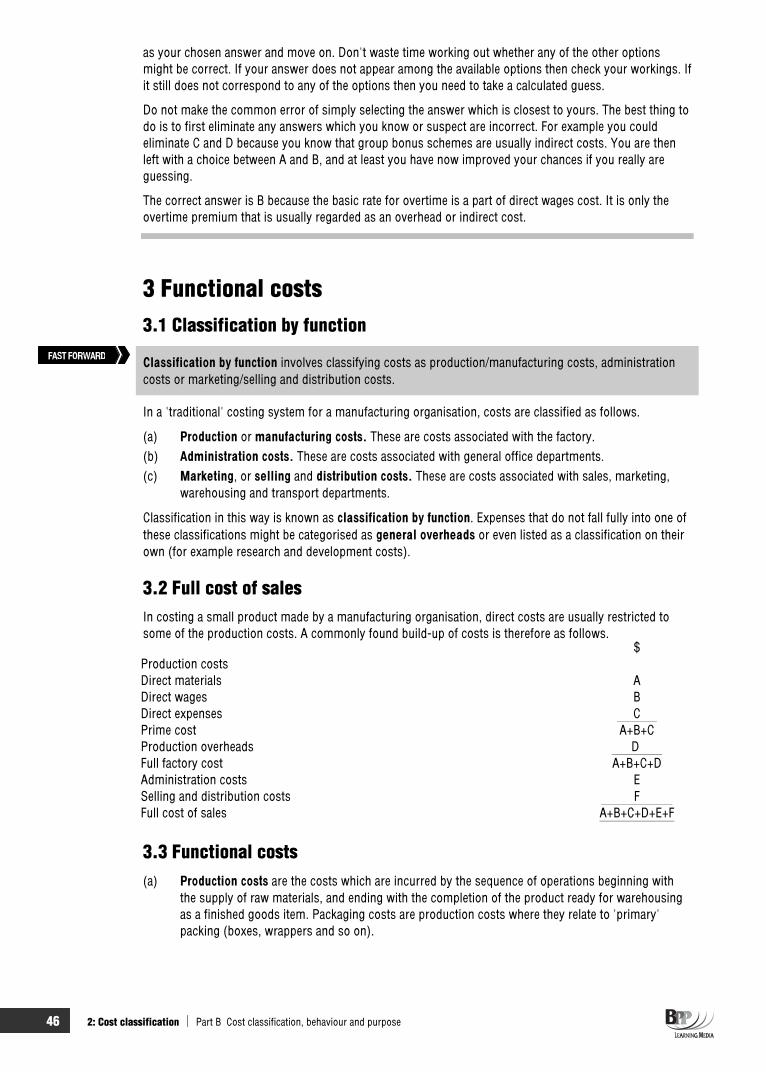
46 2: Cost classification Part B Cost classification, behaviour and purpose
as your chosen answer and move on. Don't waste time working out whether any of the other options might be correct. If your answer does not appear among the available options then check your workings. If it still does not correspond to any of the options then you need to take a calculated guess.
Do not make the common error of simply selecting the answer which is closest to yours. The best thing to do is to first eliminate any answers which you know or suspect are incorrect. For example you could eliminate C and D because you know that group bonus schemes are usually indirect costs. You are then left with a choice between A and B, and at least you have now improved your chances if you really are guessing.
The correct answer is B because the basic rate for overtime is a part of direct wages cost. It is only the overtime premium that is usually regarded as an overhead or indirect cost.
3 Functional costs 3.1 Classification by function
Classification by function involves classifying costs as production/manufacturing costs, administration costs or marketing/selling and distribution costs.
In a 'traditional' costing system for a manufacturing organisation, costs are classified as follows.
(a) Production or manufacturing costs. These are costs associated with the factory. (b) Administration costs. These are costs associated with general office departments. (c) Marketing, or selling and distribution costs. These are costs associated with sales, marketing,
warehousing and transport departments.
Classification in this way is known as classification by function. Expenses that do not fall fully into one of these classifications might be categorised as general overheads or even listed as a classification on their own (for example research and development costs).
3.2 Full cost of sales In costing a small product made by a manufacturing organisation, direct costs are usually restricted to some of the production costs. A commonly found build-up of costs is therefore as follows.
$Production costsDirect materials ADirect wages BDirect expenses CPrime cost A+B+CProduction overheads DFull factory cost A+B+C+DAdministration costs ESelling and distribution costs FFull cost of sales A+B+C+D+E+F
3.3 Functional costs (a) Production costs are the costs which are incurred by the sequence of operations beginning with
the supply of raw materials, and ending with the completion of the product ready for warehousing as a finished goods item. Packaging costs are production costs where they relate to 'primary' packing (boxes, wrappers and so on).
FAST FORWARD

Part B Cost classification, behaviour and purpose 2: Cost classification 47
(b) Administration costs are the costs of managing an organisation, that is, planning and controlling its operations, but only insofar as such administration costs are not related to the production, sales, distribution or research and development functions.
(c) Selling costs, sometimes known as marketing costs, are the costs of creating demand for products and securing firm orders from customers.
(d) Distribution costs are the costs of the sequence of operations with the receipt of finished goods from the production department and making them ready for despatch and ending with the reconditioning for reuse of empty containers.
(e) Research costs are the costs of searching for new or improved products, whereas developmentcosts are the costs incurred between the decision to produce a new or improved product and the commencement of full manufacture of the product.
(f) Financing costs are costs incurred to finance the business such as loan interest.
Question Cost classification
Within the costing system of a manufacturing company the following types of expense are incurred.
Reference number
1 Cost of oils used to lubricate production machinery 2 Motor vehicle licences for lorries 3 Depreciation of factory plant and equipment 4 Cost of chemicals used in the laboratory 5 Commission paid to sales representatives 6 Salary of the secretary to the finance director 7 Trade discount given to customers 8 Holiday pay of machine operatives 9 Salary of security guard in raw material warehouse 10 Fees to advertising agency 11 Rent of finished goods warehouse 12 Salary of scientist in laboratory 13 Insurance of the company's premises 14 Salary of supervisor working in the factory 15 Cost of typewriter ribbons in the general office 16 Protective clothing for machine operatives
Required
Complete the following table by placing each expense in the correct cost classification.
Cost classification Reference number Production costs Selling and distribution costs Administration costs Research and development costs
Each type of expense should appear only once in your answer. You may use the reference numbers in your answer.
AnswerCost classification Reference number Production costs 1 3 8 9 14 16 Selling and distribution costs 2 5 7 10 11Administration costs 6 13 15 Research and development costs 4 12

48 2: Cost classification Part B Cost classification, behaviour and purpose
4 Fixed costs and variable costs A different way of analysing and classifying costs is into fixed costs and variable costs. Many items of expenditure are part-fixed and part-variable and hence are termed semi-fixed or semi-variable costs.
A fixed cost is a cost which is incurred for a particular period of time and which, within certain activity levels, is unaffected by changes in the level of activity.
A variable cost is a cost which tends to vary with the level of activity.
4.1 Examples of fixed and variable costs (a) Direct material costs are variable costs because they rise as more units of a product are
manufactured. (b) Sales commission is often a fixed percentage of sales turnover, and so is a variable cost that
varies with the level of sales.(c) Telephone call charges are likely to increase if the volume of business expands, but there is also a
fixed element of line rental, and so they are a semi-fixed or semi-variable overhead cost.(d) The rental cost of business premises is a constant amount, at least within a stated time period, and
so it is a fixed cost.
5 Production and non-production costs
For the preparation of financial statements, costs are often classified as production costs and non-production costs. Production costs are costs identified with goods produced for resale. Non-production costs are cost deducted as expenses during the current period.
Production costs are all the costs involved in the manufacture of goods. In the case of manufactured goods, these costs consist of direct material, direct labour and manufacturing overhead.
Non-production costs are taken directly to the profit and loss account as expenses in the period in which they are incurred; such costs consist of selling and administrative expenses.
5.1 Production and non-production costs The distinction between production and non-production costs is the basis of valuing inventory.
5.2 Example A business has the following costs for a period:
$Materials 600Labour 1,000Production overheads 500Administration overheads 700
2,800
During the period 100 units are produced. If all of these costs were allocated to production units, each unit would be valued at $28.
This would be incorrect. Only production costs are allocated to units of inventory. Administrative overheads are non-production costs.
So each unit of inventory should be valued at $21((600 + 1,000 + 500)/100)
Key terms
FAST FORWARD
FAST FORWARD
Part B Cost classification, behaviour and purpose 2: Cost classification 49
This affects both gross profit and the valuation of closing inventory. If during the period 80 units are sold at $40 each, the gross profit will be:
$Sales (80 40) 3,200Cost of sales (80 21) (1,680)Gross profit 1,520
The value of closing (unsold) inventory will be $420 (20 21).
6 Other cost classifications
Avoidable costs are specific costs of an activity or business which would be avoided if the activity or business did not exist.
Unavoidable costs are costs which would be incurred whether or not an activity or sector existed.
A controllable cost is a cost which can be influenced by management decisions and actions.
An uncontrollable cost is any cost that cannot be affected by management within a given time span.
Discretionary costs are costs which are likely to arise from decisions made during the budgeting process. They are likely to be fixed amounts of money over fixed periods of time.
Examples of discretionary costs are as follows.
Advertising Training Research and Development
7 Cost units, cost objects and responsibility centres7.1 Cost centres
Cost centres are collecting places for costs before they are further analysed. Costs are further analysed into cost units once they have been traced to cost centres.
Costs consist of the costs of the following.
Direct materials Production overheads Direct labour Administration overheads Direct expenses General overheads
When costs are incurred, they are generally allocated to a cost centre. Cost centres may include the following.
A department A machine, or group of machines A project (eg the installation of a new computer system) Overhead costs eg rent, rates, electricity (which may then be allocated to departments or projects)
Cost centres are an essential 'building block' of a costing system. They are the starting point for the following.
(a) The classification of actual costs incurred. (b) The preparation of budgets of planned costs. (c) The comparison of actual costs and budgeted costs (management control).
7.2 Cost units
A cost unit is a unit of product or service to which costs can be related. The cost unit is the basic control unit for costing purposes.
Key terms
FAST FORWARD
FAST FORWARD
50 2: Cost classification Part B Cost classification, behaviour and purpose
Once costs have been traced to cost centres, they can be further analysed in order to establish a cost per cost unit. Alternatively, some items of cost may be charged directly to a cost unit, for example direct materials and direct labour costs.
Examples of cost units include the following.
Patient episode (in a hospital) Room (in a hotel) Barrel (in the brewing industry)
Question Cost units
Suggest suitable cost units which could be used to aid control within the following organisations.
(a) A hotel with 50 double rooms and 10 single rooms (b) A hospital (c) A road haulage business
Answer(a) Guest/night (b) Patient/night (c) Tonne/mile
Bed occupied/night Operation Mile Meal supplied Outpatient visit
7.3 Cost objects
A cost object is any activity for which a separate measurement of costs is desired.
If the users of management information wish to know the cost of something, this something is called a cost object. Examples include the following.
The cost of a product The cost of operating a department The cost of a service
7.4 Profit centres
Profit centres are similar to cost centres but are accountable for costs and revenues.
We have seen that a cost centre is where costs are collected. Some organisations, however, work on a profit centre basis.
Profit centre managers should normally have control over how revenue is raised and how costs are incurred. Often, several cost centres will comprise one profit centre. The profit centre manager will be able to make decisions about both purchasing and selling and will be expected to do both as profitably as possible.
A profit centre manager will want information regarding both revenues and costs. He will be judged on the profit margin achieved by his division. In practice, it may be that there are fixed costs which he cannot control, so he should be judged on contribution, which is revenue less variable costs. In this case he will want information about which products yield the highest contribution.
7.5 Revenue centres
Revenue centres are similar to cost centres and profit centres but are accountable for revenues only.Revenue centre managers should normally have control over how revenues are raised
FAST FORWARD
FAST FORWARD
FAST FORWARD

Part B Cost classification, behaviour and purpose 2: Cost classification 51
A revenue centre manager is not accountable for costs. He will be aiming purely to maximise sales revenue. He will want information on markets and new products and he will look closely at pricing and the sales performance of competitors – in addition to monitoring revenue figures.
7.6 Investment centres
An investment centre is a profit centre with additional responsibilities for capital investment and possibly for financing, and whose performance is measured by its return on investment.
An investment centre manager will take the same decisions as a profit centre manager but he also has additional responsibility for investment. So he will be judged additionally on his handling of cash surpluses and he will seek to make only those investments which yield a higher percentage than the company's notional cost of capital. So the investment centre manager will want the same information as the profit centre manager and in addition he will require quite detailed appraisals of possible investments and information regarding the results of investments already undertaken. He will have to make decisions regarding the purchase or lease of non-current assets and the investment of cash surpluses. Most of these decisions involve large sums of money.
7.7 Responsibility centres
A responsibility centre is a department or organisational function whose performance is the direct responsibility of a specific manager.
Cost centres, revenue centres, profit centres and investment centres are also known as responsibilitycentres.
Question Investment centre
Which of the following is a characteristic of an investment centre?
A Managers have control over marketing. B Management have a sales team. C Management have a sales team and are given a credit control function. D Managers can purchase capital assets.
AnswerThe correct answer is D.
This chapter has introduced a number of new terms and definitions. The topics covered in this chapter are key areas of the syllabus and are likely to be tested in the F2 – Management Accounting examination.
Exam focus point
FAST FORWARD
FAST FORWARD
52 2: Cost classification Part B Cost classification, behaviour and purpose
Chapter roundup
A direct cost is a cost that can be traced in full to the product, service or department being costed. An indirect cost (or overhead) is a cost that is incurred in the course of making a product, providing a service or running a department, but which cannot be traced directly and in full to the product, service or department.
Classification by function involves classifying costs as production/manufacturing costs, administration costs or marketing/selling and distribution costs.
A different way of analysing and classifying costs is into fixed costs and variable costs. Many items of expenditure are part-fixed and part-variable and hence are termed semi-fixed or semi-variable costs.
For the preparation of financial statements, costs are often classified as production costs and non-production costs. Production costs are costs identified with goods produced or purchased for resale. Non-production costs are costs deducted as expenses during the current period.
Cost centres are collecting places for costs before they are further analysed. Costs are further analysed into cost units once they have been traced to cost centres.
A cost unit is a unit of product or service to which costs can be related. The cost unit is the basic control unit for costing purposes.
A cost object is any activity for which a separate measurement of costs is desired.
Profit centres are similar to cost centres but are accountable for both costs and revenues.
Revenue centres are similar to cost centres and profit centres but are accountable for revenues only.
An investment centre is a profit centre with additional responsibilities for capital investment and possibly financing, and whose performance is measured by its return on investment.
A responsibility centre is a department or organisational function whose performance is the direct responsibility of a specific manager.
Quick quiz 1 Give two examples of direct expenses. 2 Give an example of an administration overhead, a selling overhead and a distribution overhead. 3 What are functional costs? 4 What is the distinction between fixed and variable costs? 5 What are production costs and non-production costs? 6 What is a cost centre? 7 What is a cost unit? 8 What is a profit centre? 9 What is an investment centre?

Part B Cost classification, behaviour and purpose 2: Cost classification 53
Answers to quick quiz 1 The hire of tools or equipment for a particular job
Maintenance costs of tools, fixtures and so on
2 Administration overhead = Depreciation of office buildings and equipment Selling overhead = Printing and stationery (catalogues, price lists) Distribution overhead = Wages of packers, drivers and despatch clerks
3 Functional costs are classified as follows.
Production or manufacturing costs Administration costs Marketing or selling and distribution costs
4 A fixed cost is a cost which is incurred for a particular period of time and which, within certain activity levels, is unaffected by changes in the level of activity.
A variable cost is a cost which tends to vary with the level of activity.
5 Production costs are costs identified with a finished product. Such costs are initially identified as part of the value of inventory. They become expenses only when the inventory is sold.
Non-production costs are costs that are deducted as expenses during the current period without ever being included in the value of inventory held.
6 A cost centre acts as a collecting place for certain costs before they are analysed further.
7 A cost unit is a unit of product or service to which costs can be related. The cost unit is the basic control unit for costing purposes.
8 A profit centre is similar to a cost centre but is accountable for costs and revenues.
9 An investment centre is a profit centre with additional responsibilities for capital investment and possibly financing.
Now try the questions below from the Exam Question Bank
Number Level Marks Time
Q2 MCQ/OTQ n/a n/a

54 2: Cost classification Part B Cost classification, behaviour and purpose

55
Cost behaviour
IntroductionSo far in this text we have introduced you to the subject of management information and explained in general terms what it is and what it does. In Chapter 2 we considered the principal methods of classifying costs. In particular, we introduced the concept of the division of costs into those that vary directly with changes in activity levels (variable costs) and those that do not (fixed costs). This chapter examines further this two-way split of costbehaviour and explains one method of splitting semi-variable costs into these two elements, the high-low method.
Topic list Syllabus reference
1 Introduction to cost behaviour B3 (b)
2 Cost behaviour patterns B3 (a)
3 Determining the fixed and variable elements of semi-variable costs
B3 (c)
56 3: Cost behaviour Part B Cost classification, behaviour and purpose
Study guide Intellectual level
B3 Fixed and variable cost
(a) Describe and illustrate graphically different types of cost behaviour 1
(b) Explain and provide examples of costs that fall into categories of fixed, stepped fixed and variable costs
1
(c) Use high-low analysis to separate the fixed and variable elements of total costs including situations involving stepped fixed costs and changes in the variable cost per unit
2
Exam guide Cost behaviour is a key area of the Management Accounting syllabus and you need to understand fixed and variable elements and the use of high-low analysis.
1 Introduction to cost behaviour 1.1 Cost behaviour and decision-making
Cost behaviour is the way in which costs are affected by changes in the volume of output.
Management decisions will often be based on how costs and revenues vary at different activity levels. Examples of such decisions are as follows.
What should the planned activity level be for the next period? Should the selling price be reduced in order to sell more units? Should a particular component be manufactured internally or bought in? Should a contract be undertaken?
1.2 Cost behaviour and cost control If the accountant does not know the level of costs which should have been incurred as a result of an organisation's activities, how can he or she hope to control costs?
1.3 Cost behaviour and budgeting Knowledge of cost behaviour is obviously essential for the tasks of budgeting, decision making and control accounting.
Remember that the behavioural analysis of costs is important for planning, control and decision-making.
1.4 Cost behaviour and levels of activity There are many factors which may influence costs. The major influence is volume of output, or the levelof activity. The level of activity may refer to one of the following.
Number of units produced Number of invoices issued Value of items sold Number of units of electricity consumed Number of items sold
Exam focus point
FAST FORWARD
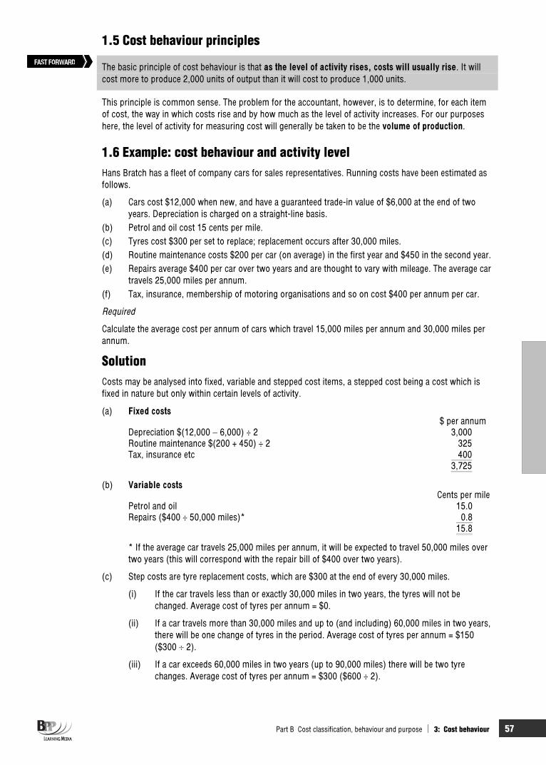
Part B Cost classification, behaviour and purpose 3: Cost behaviour 57
1.5 Cost behaviour principles
The basic principle of cost behaviour is that as the level of activity rises, costs will usually rise. It will cost more to produce 2,000 units of output than it will cost to produce 1,000 units.
This principle is common sense. The problem for the accountant, however, is to determine, for each item of cost, the way in which costs rise and by how much as the level of activity increases. For our purposes here, the level of activity for measuring cost will generally be taken to be the volume of production.
1.6 Example: cost behaviour and activity level Hans Bratch has a fleet of company cars for sales representatives. Running costs have been estimated as follows.
(a) Cars cost $12,000 when new, and have a guaranteed trade-in value of $6,000 at the end of two years. Depreciation is charged on a straight-line basis.
(b) Petrol and oil cost 15 cents per mile. (c) Tyres cost $300 per set to replace; replacement occurs after 30,000 miles. (d) Routine maintenance costs $200 per car (on average) in the first year and $450 in the second year. (e) Repairs average $400 per car over two years and are thought to vary with mileage. The average car
travels 25,000 miles per annum. (f) Tax, insurance, membership of motoring organisations and so on cost $400 per annum per car.
Required
Calculate the average cost per annum of cars which travel 15,000 miles per annum and 30,000 miles per annum.
SolutionCosts may be analysed into fixed, variable and stepped cost items, a stepped cost being a cost which is fixed in nature but only within certain levels of activity.
(a) Fixed costs$ per annum
Depreciation $(12,000 6,000) ÷ 2 3,000Routine maintenance $(200 + 450) ÷ 2 325Tax, insurance etc 400
3,725
(b) Variable costsCents per mile
Petrol and oil 15.0Repairs ($400 ÷ 50,000 miles)* 0.8
15.8
* If the average car travels 25,000 miles per annum, it will be expected to travel 50,000 miles over two years (this will correspond with the repair bill of $400 over two years).
(c) Step costs are tyre replacement costs, which are $300 at the end of every 30,000 miles.
(i) If the car travels less than or exactly 30,000 miles in two years, the tyres will not be changed. Average cost of tyres per annum = $0.
(ii) If a car travels more than 30,000 miles and up to (and including) 60,000 miles in two years, there will be one change of tyres in the period. Average cost of tyres per annum = $150 ($300 2).
(iii) If a car exceeds 60,000 miles in two years (up to 90,000 miles) there will be two tyre changes. Average cost of tyres per annum = $300 ($600 ÷ 2).
FAST FORWARD

58 3: Cost behaviour Part B Cost classification, behaviour and purpose
The estimated costs per annum of cars travelling 15,000 miles per annum and 30,000 miles per annum would therefore be as follows.
15,000 miles 30,000 milesper annum per annum
$ $Fixed costs 3,725 3,725Variable costs (15.8c per mile) 2,370 4,740Tyres – 150Cost per annum 6,095 8,615
2 Cost behaviour patterns 2.1 Fixed costs
A fixed cost is a cost which tends to be unaffected by increases or decreases in the volume of output.
Fixed costs are a period charge, in that they relate to a span of time; as the time span increases, so too will the fixed costs (which are sometimes referred to as period costs for this reason). It is important to understand that fixed costs always have a variable element, since an increase or decrease in production may also bring about an increase or decrease in fixed costs.
A sketch graph of fixed cost would look like this.
Examples of a fixed cost would be as follows.
The salary of the managing director (per month or per annum) The rent of a single factory building (per month or per annum) Straight line depreciation of a single machine (per month or per annum)
2.2 Step costs
A step cost is a cost which is fixed in nature but only within certain levels of activity.
Consider the depreciation of a machine which may be fixed if production remains below 1,000 units per month. If production exceeds 1,000 units, a second machine may be required, and the cost of depreciation (on two machines) would go up a step. A sketch graph of a step cost could look like this.
FAST FORWARD
FAST FORWARD

Part B Cost classification, behaviour and purpose 3: Cost behaviour 59
Other examples of step costs are as follows.
(a) Rent is a step cost in situations where accommodation requirements increase as output levels get higher.
(b) Basic pay of employees is nowadays usually fixed, but as output rises, more employees (direct workers, supervisors, managers and so on) are required.
(c) Royalties.
2.3 Variable costs
A variable cost is a cost which tends to vary directly with the volume of output. The variable cost per unit is the same amount for each unit produced.
A constant variable cost per unit implies that the price per unit of say, material purchased is constant, and that the rate of material usage is also constant.
(a) The most important variable cost is the cost of raw materials (where there is no discount for bulk purchasing since bulk purchase discounts reduce the cost of purchases).
(b) Direct labour costs are, for very important reasons, classed as a variable cost even though basic wages are usually fixed.
(c) Sales commission is variable in relation to the volume or value of sales. (d) Bonus payments for productivity to employees might be variable once a certain level of output is
achieved, as the following diagram illustrates.
FAST FORWARD

60 3: Cost behaviour Part B Cost classification, behaviour and purpose
Up to output A, no bonus is earned.
2.4 Non-linear or curvilinear variable costs
If the relationship between total variable cost and volume of output can be shown as a curved line on a graph, the relationship is said to be curvilinear.
Two typical relationships are as follows.
(a) (b)
Each extra unit of output in graph (a) causes a less than proportionate increase in cost whereas in graph (b), each extra unit of output causes a more than proportionate increase in cost.
The cost of a piecework scheme for individual workers with differential rates could behave in a curvilinearfashion if the rates increase by small amounts at progressively higher output levels.
2.5 Semi-variable costs (or semi-fixed costs or mixed costs)
A semi-variable/semi-fixed/mixed cost is a cost which contains both fixed and variable components and so is partly affected by changes in the level of activity.
Examples of these costs include the following.
(a) Electricity and gas bills
(i) Fixed cost = standing charge (ii) Variable cost = charge per unit of electricity used
(b) Salesman's salary
(i) Fixed cost = basic salary (ii) Variable cost = commission on sales made
(c) Costs of running a car
(i) Fixed cost = road tax, insurance (ii) Variable costs = petrol, oil, repairs (which vary with miles travelled)
2.6 Other cost behaviour patterns Other cost behaviour patterns may be appropriate to certain cost items. Examples of two other cost behaviour patterns are shown below.
FAST FORWARD
FAST FORWARD
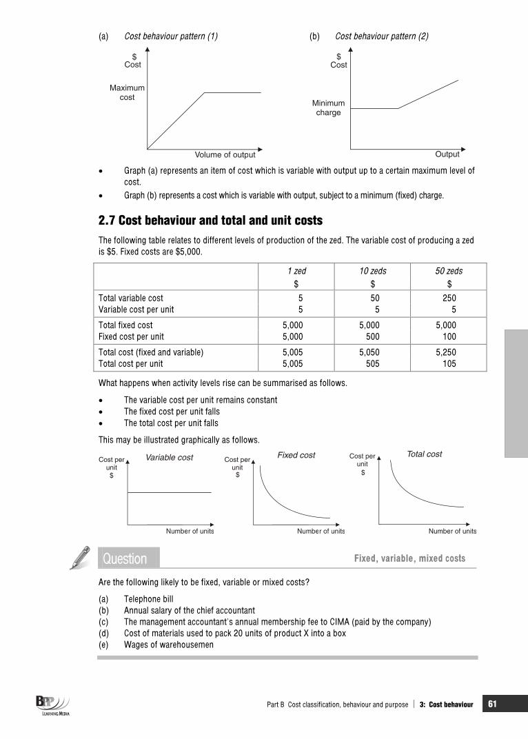
Part B Cost classification, behaviour and purpose 3: Cost behaviour 61
(a) Cost behaviour pattern (1) (b) Cost behaviour pattern (2)
Graph (a) represents an item of cost which is variable with output up to a certain maximum level of cost.
Graph (b) represents a cost which is variable with output, subject to a minimum (fixed) charge.
2.7 Cost behaviour and total and unit costsThe following table relates to different levels of production of the zed. The variable cost of producing a zed is $5. Fixed costs are $5,000.
1 zed 10 zeds 50 zeds $ $ $
Total variable cost 5 50 250Variable cost per unit 5 5 5
Total fixed cost 5,000 5,000 5,000Fixed cost per unit 5,000 500 100
Total cost (fixed and variable) 5,005 5,050 5,250Total cost per unit 5,005 505 105
What happens when activity levels rise can be summarised as follows.
The variable cost per unit remains constant The fixed cost per unit falls The total cost per unit falls
This may be illustrated graphically as follows.
Question Fixed, variable, mixed costs
Are the following likely to be fixed, variable or mixed costs?
(a) Telephone bill (b) Annual salary of the chief accountant (c) The management accountant's annual membership fee to CIMA (paid by the company) (d) Cost of materials used to pack 20 units of product X into a box (e) Wages of warehousemen

62 3: Cost behaviour Part B Cost classification, behaviour and purpose
Answer(a) Mixed (b) Fixed (c) Fixed (d) Variable (e) Variable
An exam question may give you a graph and require you to extract information from it.
2.8 Assumptions about cost behaviour Assumptions about cost behaviour include the following.
(a) Within the normal or relevant range of output, costs are often assumed to be either fixed, variableor semi-variable (mixed).
(b) Departmental costs within an organisation are assumed to be mixed costs, with a fixed and a variable element.
(c) Departmental costs are assumed to rise in a straight line as the volume of activity increases. In other words, these costs are said to be linear.
The high-low method of determining fixed and variable elements of mixed costs relies on the assumption that mixed costs are linear. We shall now go on to look at this method of cost determination.
3 Determining the fixed and variable elements of semi-variable costs
3.1 Analysing costs
The fixed and variable elements of semi-variable costs can be determined by the high-low method.
It is generally assumed that costs are one of the following.
Variable Semi-variable Fixed
Cost accountants tend to separate semi-variable costs into their variable and fixed elements. They therefore generally tend to treat costs as either fixed or variable.
There are several methods for identifying the fixed and variable elements of semi-variable costs. Each method is only an estimate, and each will produce different results. One of the principal methods is the high-low method.
3.2 High-low method Follow the steps below to estimate the fixed and variable elements of semi-variable costs.
Step 1 Review records of costs in previous periods.
Select the period with the highest activity level. Select the period with the lowest activity level.
Exam focus point
FAST FORWARD

Part B Cost classification, behaviour and purpose 3: Cost behaviour 63
Step 2 Determine the following.
Total cost at high activity level Total costs at low activity level Total units at high activity level Total units at low activity level
Step 3 Calculate the following.
level activity low at units total _ level activity high at units Totallevelactivitylowatcosttotal_levelactivity high at cost Total
= variable cost per unit (v)
Step 4 The fixed costs can be determined as follows. (Total cost at high activity level ) –(total units at high activity level × variable cost per unit)
The following graph demonstrates the high-low method.
3.3 Example: The high-low method DG Co has recorded the following total costs during the last five years. Year Output volume Total cost
Units $ 20X0 65,000 145,00020X1 80,000 162,00020X2 90,000 170,00020X3 60,000 140,00020X4 75,000 160,000
Required
Calculate the total cost that should be expected in 20X5 if output is 85,000 units.
SolutionStep 1 Period with highest activity = 20X2
Period with lowest activity = 20X3
Step 2 Total cost at high activity level = 170,000 Total cost at low activity level = 140,000 Total units at high activity level = 90,000 Total units at low activity level = 60,000
Step 3 Variable cost per unit
=level activity low at units total _ level activity high at units totallevelactivitylowatcosttotal_levelactivity high at cost total
=000,60_ 000,90000,140_ 000,170
= 000,30000,30
= $1 per unit

64 3: Cost behaviour Part B Cost classification, behaviour and purpose
Step 4 Fixed costs = (total cost at high activity level) – (total units at high activity level × variable cost per unit)
= 170,000 – (90,000 × 1) = 170,000 – 90,000 = $80,000
Therefore the costs in 20X5 for output of 85,000 units are as follows.
$Variable costs = 85,000 × $1 85,000Fixed costs 80,000
165,000
3.4 Example: The high-low method with stepped fixed costs The following data relate to the overhead expenditure of contract cleaners (for industrial cleaning) at two activity levels.
Square metres cleaned 12,750 15,100 Overheads $73,950 $83,585
When more than 14,000 square metres are industrially cleaned, there will be a step up in fixed costs of $4,700.
Required
Calculate the estimated total cost if 14,500 square metres are to be industrially cleaned.
SolutionBefore we can compare high output costs with low output costs in the normal way, we must eliminate the part of the high output costs that are due to the step up in fixed costs:
Total cost for 15,100 without step up in fixed costs = $83,585 – $4,700 = $78,885
We can now proceed in the normal way using the revised cost above.
Units $High output 15,100 Total cost 78,885Low output 12,750 Total cost 73,950 2,350 4,935
Variable cost = 2,350$4,935
= $2.10 per square metre
Before we can calculate the total cost for 14,500 square metres we need to find the fixed costs. As the fixed costs for 14,500 square metres will include the step up of $5,000, we can use the activity level of 15,100 square metres for the fixed cost calculation:
$Total cost (15,100 square metres) (this includes the step up in fixed costs) 83,585Total variable costs (15,100 x $2.10) 31,710Total fixed costs 51,875
Estimated overhead expenditure if 14,500 square metres are to be industrially cleaned: $
Fixed costs 51,875Variable costs (14,500 $2.10) 30,450
82,325

Part B Cost classification, behaviour and purpose 3: Cost behaviour 65
3.5 Example: The high-low method with a change in the variable cost per unit Same data as the previous question.
Additionally, a round of wage negotiations have just taken place which will cost an additional $1 per square metre.
SolutionEstimated overheads to clean 14,500 square metres.
Per square metre $
Variable cost 2.10 Additional variable cost 1.00Total variable cost 3.10
Cost for 14,500 square metres: $
Fixed 51,875Variable costs (14,500 $3.10) 44,950
96,825
Question High-low method
The Valuation Department of a large firm of surveyors wishes to develop a method of predicting its total costs in a period. The following past costs have been recorded at two activity levels.
Number of valuations Total cost (V) (TC)Period 1 420 82,200Period 2 515 90,275
The total cost model for a period could be represented as follows.
A TC = $46,500 + 85V C TC = $46,500 – 85V B TC = $42,000 + 95V D TC = $51,500 – 95V
AnswerThe correct answer is A.
Valuations Total costV $
Period 2 515 90,275Period 1 420 82,200Change due to variable cost 95 8,075
Variable cost per valuation = $8,075/95 = $85.
Period 2: fixed cost = $90,275 – (515 $85) = $46,500
Using good MCQ technique, you should have managed to eliminate C and D as incorrect options straightaway. The variable cost must be added to the fixed cost, rather than subtracted from it. Once you had calculated the variable cost as $85 per valuation (as shown above), you should have been able to select option A without going on to calculate the fixed cost (we have shown this calculation above for completeness).

66 3: Cost behaviour Part B Cost classification, behaviour and purpose
Chapter roundup
Cost behaviour is the way in which costs are affected by changes in the volume of output.
The basic principle of cost behaviour is that as the level of activity rises, costs will usually rise. It will cost more to produce 2,000 units of output than it will to produce 1,000 units.
A fixed cost is a cost which tends to be unaffected by increases or decreases in the volume of output.
A step cost is a cost which is fixed in nature but only within certain levels of activity.
A variable cost is a cost which tends to vary directly with the volume of output. The variable cost per unit is the same amount for each unit produced.
If the relationship between total variable cost and volume of output can be shown as a curved line on a graph, the relationship is said to be curvilinear.
A semi-variable/semi-fixed/mixed cost is a cost which contains both fixed and variable components and so is partly affected by changes in the level of activity.
The fixed and variable elements of semi-variable costs can be determined by the high-low method.
Quick quiz 1 Cost behaviour is ………………………………………………………………………………………. .
2 The basic principle of cost behaviour is that as the level of activity rises, costs will usually rise/fall.
3 Fill in the gaps for each of the graph titles below.
(a)
Graph of a ………………………..…..cost
Example:
(b)
Graph of a ………………………..…..cost
Example:

Part B Cost classification, behaviour and purpose 3: Cost behaviour 67
(c)
Graph of a ………………………..…..cost
Example:
(d)
Graph of a ………………………..…..cost
Example:
4 Costs are assumed to be either fixed, variable or semi-variable within the normal or relevant range of output.
True
False
5 The costs of operating the canteen at 'Eat a lot Company' for the past three months is as follows.
Month Cost Employees $
1 72,500 1,250 2 75,000 1,300 3 68,750 1,175
Calculate
(a) Variable cost (per employee per month) (b) Fixed cost per month

68 3: Cost behaviour Part B Cost classification, behaviour and purpose
Answers to quick quiz 1 The variability of input costs with activity undertaken.
2 Rise
3 (a) Step cost. Example: rent, supervisors' salaries (b) Variable cost. Example: raw materials, direct labour (c) Semi-variable cost. Example: electricity and telephone (d) Fixed. Example: rent, depreciation (straight-line)
4 True
5 (a) Variable cost = $50 per employee per month (b) Fixed costs = $10,000 per month
Activity Cost$
High 1,300 75,000Low 1,175 68,750
125 6,250
Variable cost per employee = $6,250/125 = $50
For 1,175 employees, total cost = $68,750
Total cost = variable cost + fixed cost $68,750 = (1,175 $50) + fixed cost
Fixed cost = $68,750 – $58,750 = $10,000
Now try the questions below from the Exam Question Bank
Number Level Marks Time
Q3 MCQ/OTQ n/a n/a

69
Business mathematics and computer spreadsheets
P
A
R
T
C

70

71
Correlation and regression; expected values
IntroductionIn chapter 3, we looked at how costs behave and how total costs can be split into fixed and variable costs using the high-low method. In this chapter, we shall be looking at another method which is used to split total costs. This method is used to determine whether there is a linear relationship between two variables. If a linear function is considered to be appropriate, regressionanalysis is used to establish the equation (this equation can then be used to make forecasts or predictions).
Topic list Syllabus reference
1 Correlation C2 (a)
2 The correlation coefficient and the coefficient of determination C2 (a)
3 Lines of best fit C2 (c)
4 Least squares method of linear regression analysis C2 (c)
5 The reliability of regression analysis forecasts C2 (b)
6 Expected values C1 (a)
7 Expectation and decision-making C1 (b) (c)

72 4: Correlation and regression; expected values Part C Business mathematics and computer spreadsheets
Study guide Intellectual level
B3 Fixed and variable costs
(a) Explain the structure of linear functions and equations 1
C1 Dealing with uncertainty
(a) Explain and calculate an expected value 1
(b) Demonstrate the use of expected values in simple decision-making situations
1
(c) Explain the limitations of the expected value technique 1
C2 Statistics for business
(a) Calculate a correlation coefficient and a coefficient of determination 1
(b) Explain and interpret coefficients calculated 1
(c) Establish a linear function using regression analysis and interpret the results 2
Exam guide This is a very important topic and it is vital that you are able to establish linear equations using regression analysis. Remember to continue to refer to the introductory chapter on basic maths if you are struggling with linear equations.
1 Correlation
1.1 Introduction
Two variables are said to be correlated if a change in the value of one variable is accompanied by a change in the value of another variable. This is what is meant by correlation.
Examples of variables which might be correlated are as follows.
A person's height and weight The distance of a journey and the time it takes to make it
1.2 Scattergraphs One way of showing the correlation between two related variables is on a scattergraph or scatterdiagram, plotting a number of pairs of data on the graph. For example, a scattergraph showing monthly selling costs against the volume of sales for a 12-month period might be as follows.
This scattergraph suggests that there is some correlation between selling costs and sales volume, so that as sales volume rises, selling costs tend to rise as well.
FAST FORWARD

Part C Business mathematics and computer spreadsheets 4: Correlation and regression; expected values 73
1.3 Degrees of correlation
Two variables might be perfectly correlated, partly correlated or uncorrelated. Correlation can be positive or negative.
The differing degrees of correlation can be illustrated by scatter diagrams.
1.3.1 Perfect correlation
All the pairs of values lie on a straight line. An exact linear relationship exists between the two variables.
1.3.2 Partial correlation
In (a), although there is no exact relationship, low values of X tend to be associated with low values of Y, and high values of X with high values of Y.
In (b) again, there is no exact relationship, but low values of X tend to be associated with high values of Y and vice versa.
1.3.3 No correlation
The values of these two variables are not correlated with each other.
1.3.4 Positive and negative correlation
Correlation, whether perfect or partial, can be positive or negative.
Positive correlation means that low values of one variable are associated with low values of the other, and high values of one variable are associated with high values of the other.
Negative correlation means that low values of one variable are associated with high values of the other, and high values of one variable with low values of the other.
Key terms
FAST FORWARD

74 4: Correlation and regression; expected values Part C Business mathematics and computer spreadsheets
2 The correlation coefficient and the coefficient of determination
2.1 The correlation coefficient
The degree of correlation between two variables is measured by the Pearsonian (product moment) correlation coefficient, r. The nearer r is to +1 or –1, the stronger the relationship.
When we have measured the degree of correlation between two variables we can decide, using actual results in the form of pairs of data, whether two variables are perfectly or partially correlated, and if they are partially correlated, whether there is a high or low degree of partial correlation.
Correlation coefficient, r = ]YY[n]XX[n
YXXYn2222
where X and Y represent pairs of data for two variables X and Y
n = the number of pairs of data used in the analysis
The formula for the correlation coefficient is given in the exam.
The correlation coefficient, r must always fall between –1 and +1. If you get a value outside this range you have made a mistake.
r = +1 means that the variables are perfectly positively correlated r = –1 means that the variables are perfectly negatively correlated r = 0 means that the variables are uncorrelated
2.2 Example: the correlation coefficient The cost of output at a factory is thought to depend on the number of units produced. Data have been collected for the number of units produced each month in the last six months, and the associated costs, as follows.
Month Output Cost '000s of units $'000
X Y 1 2 9 2 3 11 3 1 7 4 4 13 5 3 11 6 5 15
Required
Assess whether there is there any correlation between output and cost.
Solution
r = ]YY[n]XX[n
YXXYn2222
We need to find the values for the following.
(a) XY Multiply each value of X by its corresponding Y value, so that there are six values for XY. Add up the six values to get the total.
Examformula
FAST FORWARD
Exam focus point

Part C Business mathematics and computer spreadsheets 4: Correlation and regression; expected values 75
(b) X Add up the six values of X to get a total. ( X)2 will be the square of this total. (c) Y Add up the six values of Y to get a total. ( Y)2 will be the square of this total. (d) X2 Find the square of each value of X, so that there are six values for X2. Add up these values
to get a total. (e) Y2 Find the square of each value of Y, so that there are six values for Y2. Add up these values
to get a total.
Workings
X Y XY X2 Y2
2 9 18 4 81 3 11 33 9 121 1 7 7 1 49 4 13 52 16 169 3 11 33 9 121
5 15 75 25 225X = 18 Y = 66 XY = 218 X2 = 64 Y2 = 766
( X)2 = 182 = 324 ( Y)2 = 662 = 4,356
n = 6
r = 356,47666324646
6618)2186(
= 356,4596,4324384
188,1308,1
= 24060
120 =
400,14
120 =
120120
= 1
There is perfect positive correlation between the volume of output at the factory and costs which means that there is a perfect linear relationship between output and costs.
2.3 Correlation in a time series Correlation exists in a time series if there is a relationship between the period of time and the recorded value for that period of time. The correlation coefficient is calculated with time as the X variable although it is convenient to use simplified values for X instead of year numbers.
For example, instead of having a series of years 20X1 to 20X5, we could have values for X from 0 (20X1) to 4 (20X5).
Note that whatever starting value you use for X (be it 0, 1, 2 ... 721, ... 953), the value of r will always be the same.
Question Correlation
Sales of product A between 20X7 and 20Y1 were as follows.
Year Units sold ('000s) 20X7 2020X8 1820X9 1520Y0 1420Y1 11Required
Determine whether there is a trend in sales. In other words, decide whether there is any correlation between the year and the number of units sold.

76 4: Correlation and regression; expected values Part C Business mathematics and computer spreadsheets
AnswerWorkings
Let 20X7 to 20Y1 be years 0 to 4.
X Y XY X2 Y2
0 20 0 0 400 1 18 18 1 324 2 15 30 4 225 3 14 42 9 196 4 11 44 16 121
X = 10 Y = 78 XY = 134 X2 = 30 Y2 = 1,266
( X)2 = 100 ( Y)2 = 6,084
n = 5
r = 084,6266,15100305
)7810()1345(
= 084,6330,6100150
780670 =
24650110
= 300,12
110 =
90537.110110
= –0.992
There is partial negative correlation between the year of sale and units sold. The value of r is close to –1, therefore a high degree of correlation exists, although it is not quite perfect correlation. This means that there is a clear downward trend in sales.
2.4 The coefficient of determination, r2
The coefficient of determination, r2 (alternatively R2) measures the proportion of the total variation in the value of one variable that can be explained by variations in the value of the other variable.
Unless the correlation coefficient r is exactly or very nearly +1, –1 or 0, its meaning or significance is a little unclear. For example, if the correlation coefficient for two variables is +0.8, this would tell us that the variables are positively correlated, but the correlation is not perfect. It would not really tell us much else. A more meaningful analysis is available from the square of the correlation coefficient, r, which is called the coefficient of determination, r2
The question above entitled 'Correlation' shows that r = –0.992, therefore r2 = 0.984. This means that over 98% of variations in sales can be explained by the passage of time, leaving 0.016 (less than 2%) of variations to be explained by other factors.
Similarly, if the correlation coefficient between a company's output volume and maintenance costs was 0.9, r2 would be 0.81, meaning that 81% of variations in maintenance costs could be explained by variations in output volume, leaving only 19% of variations to be explained by other factors (such as the age of the equipment).
Note, however, that if r2 = 0.81, we would say that 81% of the variations in y can be explained by variations in x. We do not necessarily conclude that 81% of variations in y are caused by the variations in x. We must beware of reading too much significance into our statistical analysis.
FAST FORWARD

Part C Business mathematics and computer spreadsheets 4: Correlation and regression; expected values 77
2.5 Correlation and causation If two variables are well correlated, either positively or negatively, this may be due to pure chance or there may be a reason for it. The larger the number of pairs of data collected, the less likely it is that the correlation is due to chance, though that possibility should never be ignored entirely.
If there is a reason, it may not be causal. For example, monthly net income is well correlated with monthly credit to a person's bank account, for the logical (rather than causal) reason that for most people the one equals the other.
Even if there is a causal explanation for a correlation, it does not follow that variations in the value of one variable cause variations in the value of the other. For example, sales of ice cream and of sunglasses are well correlated, not because of a direct causal link but because the weather influences both variables.
3 Lines of best fit 3.1 Linear relationships Correlation enables us to determine the strength of any relationship between two variables but it does not offer us any method of forecasting values for one variable, Y, given values of another variable, X.
If we assume that there is a linear relationship between the two variables, however, and we determine the equation of a straight line (Y = a + bX) which is a good fit for the available data plotted on a scattergraph, we can use the equation for forecasting: we can substitute values for X into the equation and derive values for Y. If you need reminding about linear equations and graphs, refer to your Basic Maths appendix.
3.2 Estimating the equation of the line of best fit There are a number of techniques for estimating the equation of a line of best fit. We will be looking at simple linear regression analysis. This provides a technique for estimating values for a and b in the equation
Y = a + bX
where X and Y are the related variables and a and b are estimated using pairs of data for X and Y.
4 Least squares method of linear regression analysis
This section will be useful for the optional performance objective ‘Prepare financial information for management’ in your PER. Part of the key knowledge required for the fulfilment of this objective is the ability to select and apply appropriate statistical and mathematical techniques for business decision-making. Regression is a useful technique for decision-making as it can be used to determine relationships between variables which are useful for forecasting purposes.
4.1 Introduction
Linear regression analysis (the least squares method) is one technique for estimating a line of best fit. Once an equation for a line of best fit has been determined, forecasts can be made.
The least squares method of linear regression analysis involves using the following formulae for a and b in Y = a + bX.
b = 22 XXnYXXYn
Examformulae
FAST FORWARD
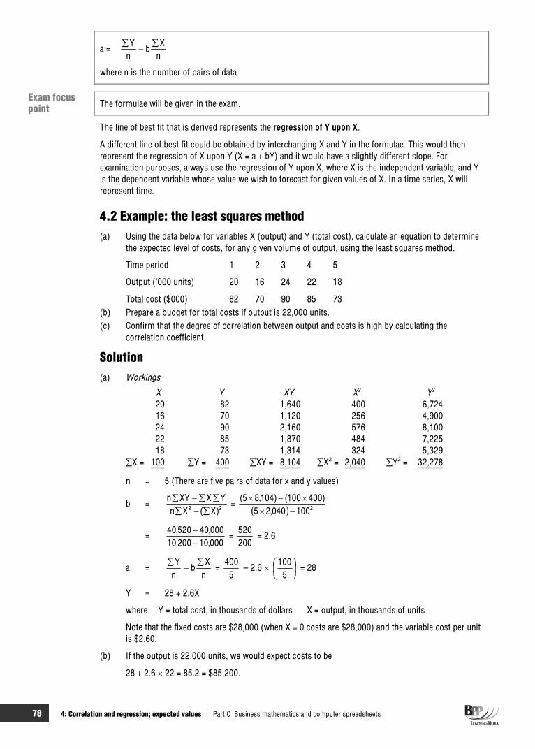
78 4: Correlation and regression; expected values Part C Business mathematics and computer spreadsheets
a = nX
bnY
where n is the number of pairs of data
The formulae will be given in the exam.
The line of best fit that is derived represents the regression of Y upon X.
A different line of best fit could be obtained by interchanging X and Y in the formulae. This would then represent the regression of X upon Y (X = a + bY) and it would have a slightly different slope. For examination purposes, always use the regression of Y upon X, where X is the independent variable, and Y is the dependent variable whose value we wish to forecast for given values of X. In a time series, X will represent time.
4.2 Example: the least squares method (a) Using the data below for variables X (output) and Y (total cost), calculate an equation to determine
the expected level of costs, for any given volume of output, using the least squares method.
Time period 1 2 3 4 5
Output (‘000 units) 20 16 24 22 18
Total cost ($000) 82 70 90 85 73 (b) Prepare a budget for total costs if output is 22,000 units. (c) Confirm that the degree of correlation between output and costs is high by calculating the
correlation coefficient.
Solution(a) Workings
X Y XY X2 Y2
20 82 1,640 400 6,72416 70 1,120 256 4,90024 90 2,160 576 8,10022 85 1,870 484 7,225
18 73 1,314 324 5,329X = 100 Y = 400 XY = 8,104 X2 = 2,040 Y2 = 32,278
n = 5 (There are five pairs of data for x and y values)
b = 22 )X(XnYXXYn
= 2100040,25)400100()104,85(
= 000,10200,10000,40520,40
= 200520
= 2.6
a = nX
bnY
= 5
400 – 2.6
5100
= 28
Y = 28 + 2.6X
where Y = total cost, in thousands of dollars X = output, in thousands of units
Note that the fixed costs are $28,000 (when X = 0 costs are $28,000) and the variable cost per unit is $2.60.
(b) If the output is 22,000 units, we would expect costs to be
28 + 2.6 22 = 85.2 = $85,200.
Exam focus point

Part C Business mathematics and computer spreadsheets 4: Correlation and regression; expected values 79
(c) r = 2400278,325200
520 =
390,1200520
= 3.527
520 = +0.99
4.3 Regression lines and time series The same technique can be applied to calculate a regression line (a trend line) for a time series. This is particularly useful for purposes of forecasting. As with correlation, years can be numbered from 0 upwards.
Question Trend line
Using the data in the question entitled 'Correlation', calculate the trend line of sales and forecast sales in 20Y2 and 20Y3.
AnswerUsing workings from the question entitled 'Correlation':
b = 21030578101345
= 100150780670
= –2.2
a = nX
bnY
= 5
102.2578
= 20
Y = 20 – 2.2X where X = 0 in 20X7, X = 1 in 20X8 and so on.
Using the trend line, predicted sales in 20Y2 (year 5) would be:
20 – (2.2 5) = 9 ie 9,000 units
and predicated sales in 20Y3 (year 6) would be:
20 – (2.2 6) = 6.8 ie 6,800 units.
Question Regression analysis
Regression analysis was used to find the equation Y = 300 – 4.7X, where X is time (in quarters) and Y is sales level in thousands of units. Given that X = 0 represents 20X0 quarter 1 what are the forecast sales levels for 20X5 quarter 4?
AnswerX = 0 corresponds to 20X0 quarter 1
Therefore X = 23 corresponds to 20X5 quarter 4
Forecast sales = 300 – (4.7 × 23) = 191.9 = 191,900 units
Question Forecasting
Over a 36 month period sales have been found to have an underlying regression line of Y = 14.224 + 7.898X where Y is the number of items sold and X represents the month.
What are the forecast number of items to be sold in month 37?

80 4: Correlation and regression; expected values Part C Business mathematics and computer spreadsheets
AnswerY = 14.224 + 7.898X = 14.224 + (7.898 × 37) = 306.45 = 306 units
5 The reliability of regression analysis forecasts As with all forecasting techniques, the results from regression analysis will not be wholly reliable. There are a number of factors which affect the reliability of forecasts made using regression analysis.
(a) It assumes a linear relationship exists between the two variables (since linear regression analysis produces an equation in the linear format) whereas a non-linear relationship might exist.
(b) It assumes that the value of one variable, Y, can be predicted or estimated from the value of one other variable, X. In reality the value of Y might depend on several other variables, not just X.
(c) When it is used for forecasting, it assumes that what has happened in the past will provide a reliable guide to the future.
(d) When calculating a line of best fit, there will be a range of values for X. In the example in Paragraph 4.2, the line Y = 28 + 2.6X was predicted from data with output values ranging from X = 16 to X = 24. Depending on the degree of correlation between X and Y, we might safely use the estimated line of best fit to predict values for Y in the future, provided that the value of X remains within the range 16 to 24. We would be on less safe ground if we used the formula to predict a value for Y when X = 10, or 30, or any other value outside the range 16 to 24, because we would have to assume that the trend line applies outside the range of X values used to establish the line in the first place.
(i) Interpolation means using a line of best fit to predict a value within the two extreme points of the observed range.
(ii) Extrapolation means using a line of best fit to predict a value outside the two extreme points.
When linear regression analysis is used for forecasting a time series (when the X values represent time) it assumes that the trend line can be extrapolated into the future. This might not necessarily be a good assumption to make.
(e) As with any forecasting process, the amount of data available is very important. Even if correlation is high, if we have fewer than about ten pairs of values, we must regard any forecast as being somewhat unreliable. (It is likely to provide more reliable forecasts than the scattergraph method, however, since it uses all of the available data.)
(f) The reliability of a forecast will depend on the reliability of the data collected to determine the regression analysis equation. If the data is not collected accurately or if data used is false, forecasts are unlikely to be acceptable.
A check on the reliability of the estimated line Y= 28 + 2.6X can be made, however, by calculating the coefficient of correlation. From the answer to the example in Paragraph 4.2, we know that r = 0.99. This is a high positive correlation, and r2 = 0.9801, indicating that 98.01% of the variation in cost can be explained by the variation in volume. This would suggest that a fairly large degree of reliance canprobably be placed on estimates .
If there is a perfect linear relationship between X and Y (r = 1) then we can predict Y from any given value of X with great confidence.
FAST FORWARD

Part C Business mathematics and computer spreadsheets 4: Correlation and regression; expected values 81
If correlation is high (for example r = 0.9) the actual values will all lie quite close to the regression line and so predictions should not be far out. If correlation is below about 0.7, predictions will only give a very rough guide as to the likely value of Y.
6 Expected values
At the ACCA Teachers’ Conference in 2009, the examiner specifically mentioned that students struggled with syllabus area C1 which is covered in this section and section 7. You will notice that there are two past exam questions included – one in this section and one in section 7. Neither question was answered correctly by more than one third of students. You are advised to study sections 6 and 7 carefully before attempting the questions.
An expected value (or EV) is a weighted average value, based on probabilities. The expected value for a single event can offer a helpful guide for management decisions.
6.1 How to calculate expected values If the probability of an outcome of an event is p, then the expected number of times that this outcome will occur in n events (the expected value) is equal to n p.
For example, suppose that the probability that a transistor is defective is 0.02. How many defectives would we expect to find in a batch of 4,000 transistors?
EV = 4,000 0.02 = 80 defectives
6.2 Example: Expected values The daily sales of Product T may be as follows.
Units Probability1,000 0.22,000 0.33,000 0.44,000 0.1
1.0Required
Calculate the expected daily sales.
SolutionThe EV of daily sales may be calculated by multiplying each possible outcome (volume of daily sales) by the probability that this outcome will occur.
Probability Expected valueUnits Units1,000 0.2 2002,000 0.3 6003,000 0.4 1,2004,000 0.1 400
EV of daily sales 2,400
In the long run the expected value should be approximately the actual average, if the event occurs many times over. In the example above, we do not expect sales on any one day to equal 2,400 units, but in the long run, over a large number of days, average sales should equal 2,400 units a day.
Exam focus point
FAST FORWARD

82 4: Correlation and regression; expected values Part C Business mathematics and computer spreadsheets
6.3 Expected values and single events The point made in the preceding paragraph is an important one. An expected value can be calculated when the event will only occur once or twice, but it will not be a true long-run average of what will actually happen, because there is no long run.
6.4 Example: Expected values and single events Suppose, for example, that a businessman is trying to decide whether to invest in a project. He estimates that there are three possible outcomes.
Outcome Profit/(loss) Probability $
Success 10,000 0.2 Moderate success 2,000 0.7Failure (4,000) 0.1
The expected value of profit may be calculated as follows.
Profit/(loss) Probability Expected value$ $
10,000 0.2 2,0002,000 0.7 1,400
(4,000) 0.1 (400)Expected value of profit 3,000
In this example, the project is a one-off event, and as far as we are aware, it will not be repeated. The actual profit or loss will be $10,000, $2,000 or $(4,000), and the average value of $3,000 will not actually happen. There is no long-run average of a single event.
Nevertheless, the expected value can be used to help the manager decide whether or not to invest in the project.
Question Expected values 1
A company manufactures and sells product D. The selling price of the product is $6 per unit, and estimates of demand and variable costs of sales are as follows.
Variable costProbability Demand Probability per unit Units $ 0.3 5,000 0.1 3.00 0.6 6,000 0.3 3.50 0.1 8,000 0.5 4.00
0.1 4.50
The unit variable costs do not depend on the volume of sales.
Fixed costs will be $10,000.
Required
Calculate the expected profit.

Part C Business mathematics and computer spreadsheets 4: Correlation and regression; expected values 83
AnswerThe EV of demand is as follows.
Demand Probability Expected valueUnits Units5,000 0.3 1,5006,000 0.6 3,6008,000 0.1 800
EV of demand 5,900
The EV of the variable cost per unit is as follows.
Variable costs Probability Expected value $ $ 3.00 0.1 0.30 3.50 0.3 1.05 4.00 0.5 2.00 4.50 0.1 0.45
EV of unit variable costs 3.80
$Sales 5,900 units × $6.00 35,400Less: variable costs 5,900 units × $3.80 22,420Contribution 12,980Less: fixed costs 10,000Expected profit 2,980
Question Expected values 2
The probability of an organisation making a profit of $180,000 next month is half the probability of it making a profit of $75,000.
What is the expected profit for next month?
A $110,000 C $145,000 B $127,500 D $165,000
AnswerThe correct answer is A.
180,000 1 75,000 2
1 2= $110,000
This is a question from the December 2007 paper and less than 30% of students answered this correctly.Many students answered B, which weights the two profits equally rather than in the ratio given in the question.
6.5 The expected value equation The expected value is summarised in equation form as follows.
)x(xP)x(E
This is read as 'the expected value of a particular outcome "x" is equal to the sum of the products of each value of x and the corresponding probability of that value of x occurring'.
Exam focus point

84 4: Correlation and regression; expected values Part C Business mathematics and computer spreadsheets
7 Expectation and decision-making 7.1 Decision-making
Probability and expectation should be seen as an aid to decision-making.
The concepts of probability and expected value are vital in business decision-making. The expected values for single events can offer a helpful guide for management decisions.
A project with a positive EV should be accepted A project with a negative EV should be rejected
Another decision rule involving expected values that you are likely to come across is the choice of an option or alternative which has the highest EV of profit (or the lowest EV of cost).
Choosing the option with the highest EV of profit is a decision rule that has both merits and drawbacks, as the following simple example will show.
7.2 Example: The expected value criterion Suppose that there are two mutually exclusive projects with the following possible profits.
Project A Project B Probability Profit Probability Profit/(loss)
$ $ 0.8 5,000 0.1 (2,000) 0.2 6,000 0.2 5,000
0.6 7,000 0.1 8,000
Required
Determine which project should be chosen.
SolutionThe EV of profit for each project is as follows.
$(a) Project A (0.8 5,000) + (0.2 6,000) = 5,200 (b) Project B (0.1 (2,000)) + (0.2 5,000) + (0.6 7,000) + (0.1 8,000) = 5,800
Project B has a higher EV of profit. This means that on the balance of probabilities, it could offer a better return than A, and so is arguably a better choice.
On the other hand, the minimum return from project A would be $5,000 whereas with B there is a 0.1 chance of a loss of $2,000. So project A might be a safer choice.
Question Expected values 3
A company is deciding whether to invest in a project. There are three possible outcomes of the investment:
Outcome Profit/(Loss)$'000
Optimistic 19.2Most likely 12.5Pessimistic (6.7)
There is a 30% chance of the optimistic outcome, and a 60% chance of the most likely outcome arising. The expected value of profit from the project is
A $7,500 C $13,930 B $12,590 D $25,000
FAST FORWARD
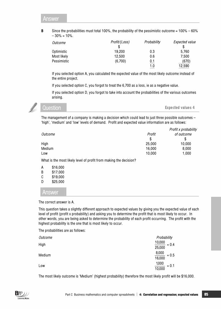
Part C Business mathematics and computer spreadsheets 4: Correlation and regression; expected values 85
Answer
B Since the probabilities must total 100%, the probability of the pessimistic outcome = 100% – 60% – 30% = 10%.
Outcome Profit/(Loss) Probability Expected value$ $
Optimistic 19,200 0.3 5,760Most likely 12,500 0.6 7,500Pessimistic (6,700) 0.1 (670)
1.0 12,590
If you selected option A, you calculated the expected value of the most likely outcome instead of the entire project.
If you selected option C, you forgot to treat the 6,700 as a loss, ie as a negative value.
If you selected option D, you forgot to take into account the probabilities of the various outcomes arising.
Question Expected values 4
The management of a company is making a decision which could lead to just three possible outcomes – ‘high’, ‘medium’ and ‘low’ levels of demand. Profit and expected value information are as follows:
Profit x probability Outcome Profit of outcome
$ $High 25,000 10,000Medium 16,000 8,000Low 10,000 1,000
What is the most likely level of profit from making the decision?
A $16,000 B $17,000 C $19,000 D $25,000
AnswerThe correct answer is A.
This question takes a slightly different approach to expected values by giving you the expected value of each level of profit (profit x probability) and asking you to determine the profit that is most likely to occur. In other words, you are being asked to determine the probability of each profit occurring. The profit with the highest probability is the one that is most likely to occur.
The probabilities are as follows:
Outcome Probability
High000,25000,10
= 0.4
Medium000,16000,8
= 0.5
Low000,10
000,1 = 0.1
The most likely outcome is ‘Medium’ (highest probability) therefore the most likely profit will be $16,000.

86 4: Correlation and regression; expected values Part C Business mathematics and computer spreadsheets
This question appeared in the June 2008 exam and was answered correctly by less than one third of candidates. Choices B, C and D were all popular answers. Choice B was the simple average of the three profit figures and choice C was the expected profit (the sum of the expected values). Choice D was the highest level of profit.
7.3 Payoff tables Decisions have to be taken about a wide variety of matters (capital investment, controls on production, project scheduling and so on) and under a wide variety of conditions from virtual certainty to completeuncertainty.
There are, however, certain common factors in many business decisions.
(a) When a decision has to be made, there will be a range of possible actions.(b) Each action will have certain consequences, or payoffs (for example, profits, costs, time). (c) The payoff from any given action will depend on the circumstances (for example, high demand or
low demand), which may or may not be known when the decision is taken. Frequently each circumstance will be assigned a probability of occurrence. The circumstances are not dependent on the action taken.
For a decision with these elements, a payoff table can be prepared.
A payoff table is simply a table with rows for circumstances and columns for actions (or vice versa), and the payoffs in the cells of the table.
For example, a decision on the level of advertising expenditure to be undertaken given different states of the economy, would have payoffs in $'000 of profit after advertising expenditure as follows.
Actions: expenditure High Medium Low
Circumstances: Boom +50 +30 +15the state of the Stable +20 +25 +5 economy Recession 0 –10 –35
Question Pay off tables
In a restaurant there is a 30% chance of five apple pies being ordered a day and a 70% chance of ten being ordered. Each apple pie sells for $2. It costs $1 to make an apple pie. Using a payoff table, decide how many apple pies the restaurant should prepare each day, bearing in mind that unsold apple pies must be thrown away at the end of each day.
Answer
PreparedFive Ten
Demand Five (P = 0.3) 5 0 Ten (P = 0.7) 5 10
Prepare five, profit = ($5 0.3) + ($5 0.7) = $5 Prepare ten, profit = ($0 0.3) + ($10 0.7) = $7
Ten pies should be prepared.
Exam focus point
FAST FORWARD
Part C Business mathematics and computer spreadsheets 4: Correlation and regression; expected values 87
7.4 Limitations of expected values Evaluating decisions by using expected values have a number of limitations.
(a) The probabilities used when calculating expected values are likely to be estimates. They may therefore be unreliable or inaccurate.
(b) Expected values are long-term averages and may not be suitable for use in situations involving one-off decisions. They may therefore be useful as a guide to decision making.
(c) Expected values do not consider the attitudes to risk of the people involved in the decision-making process. They do not, therefore, take into account all of the factors involved in the decision.
(d) The time value of money may not be taken into account: $100 now is worth more than $100 in ten years' time.
Chapter roundup
Two variables are said to be correlated if a change in the value of one variable is accompanied by a change in the value of another variable. This is what is meant by correlation.
Two variables might be perfectly correlated, partly correlated or uncorrelated. Correlation can be positive or negative.
The degree of correlation between two variables is measured by the Pearsonian (product moment) correlation coefficient, r. The nearer r is to +1 or –1, the stronger the relationship.
The coefficient of determination, r2(alternatively R2) measures the proportion of the total variation in the value of one variable that can be explained by variations in the value of the other variable.
Linear regression analysis (the least squares method) is one technique for estimating a line of best fit. Once an equation for a line of best fit has been determined, forecasts can be made.
As with all forecasting techniques, the results from regression analysis will not be wholly reliable. There are a number of factors which affect the reliability of forecasts made using regression analysis.
An expected value (or EV) is a weighted average value, based on probabilities. The expected value for a single event can offer a helpful guide for management decisions.
Probability and expectation should be seen as an aid to decision making.
A payoff table is simply a table with rows for circumstances and columns for actions (or vice versa) and the payoffs in the cells of the table.
Quick quiz 1 ……………….. means that low values of one variable are associated with low values of the other, and
high values of one variable are associated with high values of the other.
2 ……………….. means that low values of one variable are associated with high values of the other, and high values of one variable with low values of the other.
3 (a) Perfect positive correlation, r = ……………….. (b) Perfect negative correlation, r = ……………….. (c) No correlation, r = ………………..
The correlation coefficient, r, must always fall within the range ……………….. to ……………….. .
4 If the correlation coefficient of a set of data is 0.9, what is the coefficient of determination and how is it interpreted?

88 4: Correlation and regression; expected values Part C Business mathematics and computer spreadsheets
5 (a) The equation of a straight line is given as Y = a + bX. Give two methods used for estimating the above equation.
(b) If Y = a + bX, it is best to use the regression of Y upon X where X is the dependent variable and Y is the independent variable.
True
False
6 List five factors affecting the reliability of regression analysis forecasts.
7 What is an expected value?
Answers to quick quiz 1 Positive correlation
2 Negative correlation
3 (a) r = +1 (b) r = –1 (c) r = 0
The correlation coefficient, r, must always fall within the range –1 to +1.
4 Correlation coefficient = r = 0.9
Coefficient of determination = r2 = 0.92 = 0.81 or 81%
This tells us that over 80% of the variations in the dependent variable (Y) can be explained by variations in the independent variable, X.
5 (a) (i) Scattergraph method (line of best fit) (ii) Simple linear regression analysis
(b) False. When using the regression of Y upon X, X is the independent variable and Y is the dependent variable (the value of Y will depend upon the value of X).
6 (a) It assumes a linear relationship exists between the two variables. (b) It assumes that the value of one variable, Y, can be predicted or estimated from the value of
another variable, X. (c) It assumes that what happened in the past will provide a reliable guide to the future. (d) It assumes that the trend line can be extrapolated into the future. (e) The amount of data available.
7 A weighted average value based on probabilities.
Now try the questions below from the Exam Question Bank
Number Level Marks Time
Q4 MCQ n/a n/a

89
Spreadsheets
IntroductionSpreadsheet skills are essential for people working in a management accounting environment as much of the information produces is analysed or presented using spreadsheet software.
This chapter will look at features and functions of commonly used spreadsheet software, its advantages and its disadvantages and how it is used in the day-to-day work of an accountant.
This is a long chapter with a high level of detail. If you are comfortable with using spreadsheets – for example, if you use them extensively at work – you can probably skim over this chapter quite quickly.
Topic list Syllabus reference
1 Features and functions of spreadsheets C3 (a)
2 Examples of spreadsheet formula C3 (a)
3 Basic skills C3 (b)
4 Spreadsheet construction C3 (b)
5 Formulae with conditions C3 (b)
6 Charts and graphs C3 (b)
7 Spreadsheet format and appearance C3 (b)
8 Other issues C3 (b)
9 Three dimensional (multi-sheet) spreadsheets C3 (b)
10 Macros C3 (a)
11 Advantages and disadvantages of spreadsheet software C3 (c)
12 Uses of spreadsheet software C3 (c)

90 5: Spreadsheets Part C Business mathematics and computer spreadsheets
Study guide Intellectual level
C3 Use of spreadsheet models
(a) Explain the role and features of a spreadsheet system 1
(b) Demonstrate a basic understanding of the use of spreadsheets 1
(c) Identify applications for spreadsheets in cost and management accounting 1
Exam guide This topic will account for no more than about 4 marks in the examination and if you are familiar with spreadsheets you may want to skip a lot of this chapter. We have covered this topic in some depth as an aid to those students who do not normally use spreadsheets.
One of the essential PER performance objectives requires you to demonstrate that you can use information and communications technology. You can contribute towards the fulfilment of this objective by showing that you can use formulae, functions and tools to manipulate, analyse and interpret data. The information contained in this chapter can be put into practice in the workplace and will therefore help you towards gaining the skills you need to fulfil this essential objective.
1 Features and functions of spreadsheets Use of spreadsheets is an essential part of the day-to-day work of an accountant.
1.1 What is a spreadsheet?
A spreadsheet is an electronic piece of paper divided into rows and columns. The intersection of a row and a column is known as a cell.
A spreadsheet is divided into rows (horizontal) and columns (vertical). The rows are numbered 1, 2, 3 . . . etc and the columns lettered A, B C . . . etc. Each individual area representing the intersection of a row and a column is called a 'cell'. A cell address consists of its row and column reference. For example, in the spreadsheet below the word ‘Jan’ is in cell B2. The cell that the cursor is currently in or over is known as the 'active cell'.
The main examples of spreadsheet packages are Lotus 1 2 3 and Microsoft Excel. We will be referring to Microsoft Excel, as this is the most widely-used spreadsheet. A simple Microsoft Excel spreadsheet, containing budgeted sales figures for three geographical areas for the first quarter of the year, is shown below.
1.2 Why use spreadsheets? Spreadsheets provide a tool for calculating, analysing and manipulating numerical data. Spreadsheets make the calculation and manipulation of data easier and quicker. For example, the spreadsheet above has
FAST FORWARD
FAST FORWARD
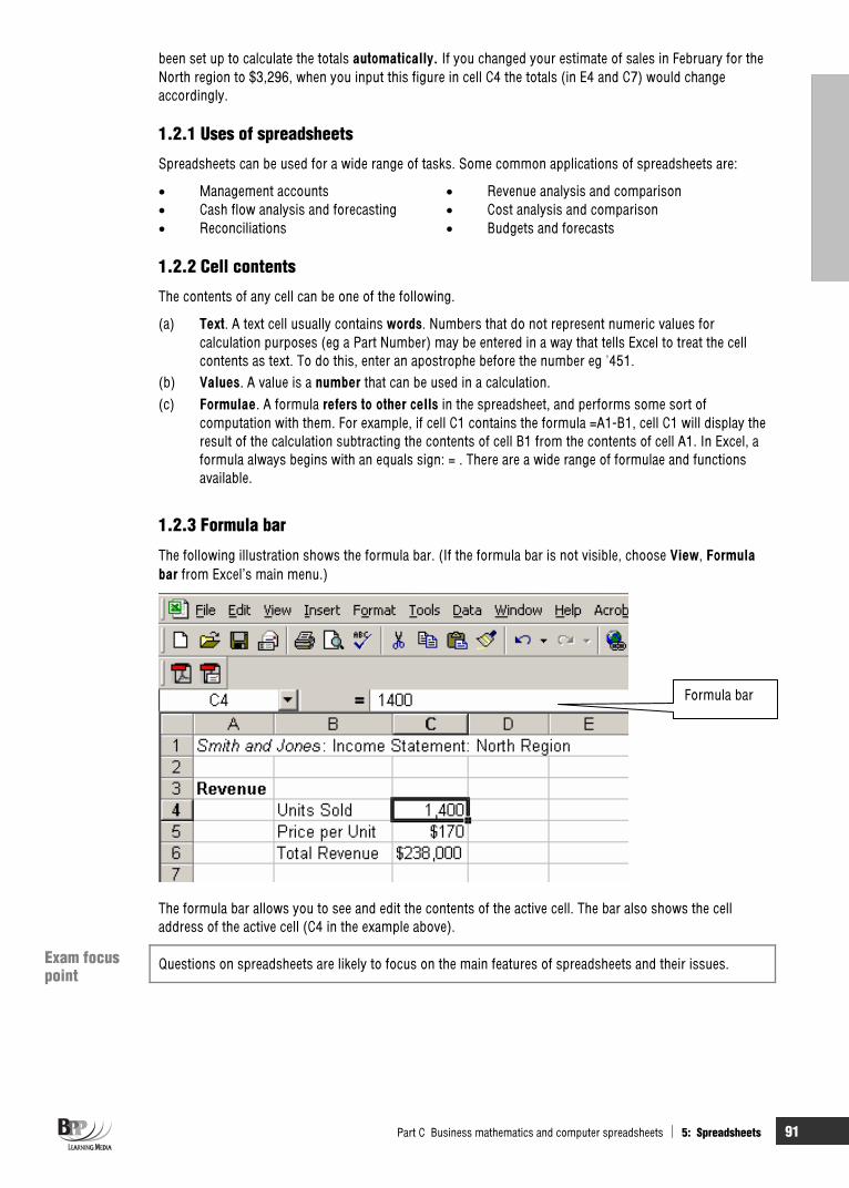
Part C Business mathematics and computer spreadsheets 5: Spreadsheets 91
been set up to calculate the totals automatically. If you changed your estimate of sales in February for the North region to $3,296, when you input this figure in cell C4 the totals (in E4 and C7) would change accordingly.
1.2.1 Uses of spreadsheets
Spreadsheets can be used for a wide range of tasks. Some common applications of spreadsheets are:
Management accounts Revenue analysis and comparison Cash flow analysis and forecasting Cost analysis and comparison Reconciliations Budgets and forecasts
1.2.2 Cell contents
The contents of any cell can be one of the following.
(a) Text. A text cell usually contains words. Numbers that do not represent numeric values for calculation purposes (eg a Part Number) may be entered in a way that tells Excel to treat the cell contents as text. To do this, enter an apostrophe before the number eg '451.
(b) Values. A value is a number that can be used in a calculation. (c) Formulae. A formula refers to other cells in the spreadsheet, and performs some sort of
computation with them. For example, if cell C1 contains the formula =A1-B1, cell C1 will display the result of the calculation subtracting the contents of cell B1 from the contents of cell A1. In Excel, a formula always begins with an equals sign: = . There are a wide range of formulae and functions available.
1.2.3 Formula bar
The following illustration shows the formula bar. (If the formula bar is not visible, choose View, Formulabar from Excel’s main menu.)
The formula bar allows you to see and edit the contents of the active cell. The bar also shows the cell address of the active cell (C4 in the example above).
Questions on spreadsheets are likely to focus on the main features of spreadsheets and their issues.
Formula bar
Exam focus point
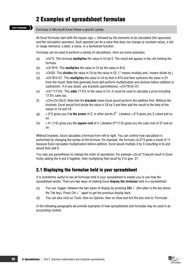
92 5: Spreadsheets Part C Business mathematics and computer spreadsheets
2 Examples of spreadsheet formulae Formulas in Microsoft Excel follow a specific syntax.
All Excel formulae start with the equals sign =, followed by the elements to be calculated (the operands) and the calculation operators. Each operand can be a value that does not change (a constant value), a cell or range reference, a label, a name, or a worksheet function.
Formulae can be used to perform a variety of calculations. Here are some examples.
(a) =C4*5. This formula multiplies the value in C4 by 5. The result will appear in the cell holding the formula.
(b) =C4*B10. This multiplies the value in C4 by the value in B10. (c) =C4/E5. This divides the value in C4 by the value in E5. (* means multiply and / means divide by.) (d) =C4*B10-D1. This multiplies the value in C4 by that in B10 and then subtracts the value in D1
from the result. Note that generally Excel will perform multiplication and division before addition or subtraction. If in any doubt, use brackets (parentheses): =(C4*B10)–D1.
(e) =C4*117.5%. This adds 17.5% to the value in C4. It could be used to calculate a price including 17.5% sales tax.
(f) =(C4+C5+C6)/3. Note that the brackets mean Excel would perform the addition first. Without the brackets, Excel would first divide the value in C6 by 3 and then add the result to the total of the values in C4 and C5.
(g) = 2^2 gives you 2 to the power of 2, in other words 22 . Likewise = 2^3 gives you 2 cubed and so on.
(h) = 4^ (1/2) gives you the square root of 4. Likewise 27^(1/3) gives you the cube root of 27 and so on.
Without brackets, Excel calculates a formula from left to right. You can control how calculation is performed by changing the syntax of the formula. For example, the formula =5+2*3 gives a result of 11 because Excel calculates multiplication before addition. Excel would multiply 2 by 3 (resulting in 6) and would then add 5.
You may use parentheses to change the order of operations. For example =(5+2)*3 would result in Excel firstly adding the 5 and 2 together, then multiplying that result by 3 to give 21.
2.1 Displaying the formulae held in your spreadsheet It is sometimes useful to see all formulae held in your spreadsheet to enable you to see how the spreadsheet works. There are two ways of making Excel display the formulae held in a spreadsheet.
(a) You can 'toggle' between the two types of display by pressing Ctrl +` (the latter is the key above the Tab key). Press Ctrl + ` again to get the previous display back.
(b) You can also click on Tools, then on Options, then on View and tick the box next to ‘Formulas’.
In the following paragraphs we provide examples of how spreadsheets and formulae may be used in an accounting context.
FAST FORWARD

Part C Business mathematics and computer spreadsheets 5: Spreadsheets 93
2.1.1 Example: formulae
(a) In the spreadsheet shown above, which of the cells have had a number typed in, and which cells display the result of calculations (ie which cells contain a formula)?
(b) What formula would you put in each of the following cells?
(i) Cell B7 (ii) Cell E6 (iii) Cell E7
(c) If the February sales figure for the South changed from $5,826 to $5,731, what other figures would change as a result? Give cell references.
Solution(a) Cells into which you would need to enter a value are: B4, B5, B6, C4, C5, C6, D4, D5 and D6. Cells
which would perform calculations are B7, C7, D7, E4, E5, E6 and E7.
(b) (i) =B4+B5+B6 or better =SUM(B4:B6)(ii) =B6+C6+D6 or better =SUM(B6:D6)(iii) =E4+E5+E6 or better =SUM(E4:E6) Alternatively, the three monthly totals could be added
across the spreadsheet: = SUM (B7: D7)
(c) The figures which would change, besides the amount in cell C5, would be those in cells C7, E5 and E7. (The contents of E7 would change if any of the sales figures changed.)
Question SUM formulae
The following spreadsheet shows sales of two products, the Ego and the Id, for the period July to September.
Devise a suitable formula for each of the following cells.
(a) Cell B7 (c) Cell E7 (b) Cell E6
Answer(a) =SUM(B5:B6) (c) =SUM (E5:E6) or =SUM(B7:D7) (b) =SUM(B6:D6)

94 5: Spreadsheets Part C Business mathematics and computer spreadsheets
or (best of all) =IF(SUM(E5:E6) =SUM(B7:D7),SUM(B7:D7),"ERROR") Don't worry if you don't understand this formula when first attempting this question – we cover IF statements later in this chapter.
Question Formulae
The following spreadsheet shows sales, exclusive of sales tax, in row 6.
Your manager has asked you to insert formulae to calculate sales tax at 17½% in row 7 and also to produce totals.
(a) Devise a suitable formula for cell B7 and cell E8. (b) How could the spreadsheet be better designed?
Answer(a) For cell B7 =B6*0.175 For cell E8 =SUM(E6:E7)
(b) By using a separate 'variables' holding the sales tax rate and possibly the Sales figures. The formulae could then refer to these cells as shown below.
3 Basic skills
Essential basic skills include how to move around within a spreadsheet, how to enter and edit data, how to fill cells, how to insert and delete columns and rows and how to improve the basic layout andappearance of a spreadsheet.
In this section we explain some basic spreadsheeting skills. We give instructions for Microsoft Excel, the most widely used package. Our examples should be valid with all versions of Excel released since 1997.
You should read this section while sitting at a computer and trying out the skills we describe 'hands-on'.
3.1 Moving about The F5 key is useful for moving around within large spreadsheets. If you press the function key F5, a GoTo dialogue box will allow you to specify the cell address you would like to move to. Try this out.
Also experiment by holding down Ctrl and pressing each of the direction arrow keys in turn to see where you end up. Try using the Page Up and Page Down keys and also try Home and End and Ctrl + these keys.
FAST FORWARD

Part C Business mathematics and computer spreadsheets 5: Spreadsheets 95
Try Tab and Shift + Tab, too. These are all useful shortcuts for moving quickly from one place to another in a large spreadsheet.
3.2 Editing cell contents Suppose cell A2 currently contains the value 456. If you wish to change the entry in cell A2 from 456 to 123456 there are four options – as shown below.
(a) Activate cell A2, type 123456 and press Enter.
To undo this and try the next option press Ctrl + Z: this will always undo what you have just done.
(b) Double-click in cell A2. The cell will keep its thick outline but you will now be able to see a vertical line flashing in the cell. You can move this line by using the direction arrow keys or the Home and the End keys. Move it to before the 4 and type 123. Then press Enter.
When you have tried this press Ctrl + Z to undo it.
(c) Click once before the number 456 in the formula bar. Again you will get the vertical line and you can type in 123 before the 4. Then press Enter. Undo this before moving onto (d).
(d) Press the function key F2. The vertical line cursor will be flashing in cell A2 at the end of the figures entered there (after the 6). Press Home to get to a position before the 4 and then type in 123 and press Enter, as before.
3.3 Deleting cell contents You may delete the contents of a cell simply by making the cell the active cell and then pressing Delete.The contents of the cell will disappear. You may also highlight a range of cells to delete and then delete the contents of all cells within the range.
For example, enter any value in cell A1 and any value in cell A2. Move the cursor to cell A2. Now hold down the Shift key (the one above the Ctrl key) and keeping it held down press the arrow. Cell A2 will stay white but cell A1 will go black. What you have done here is selected the range A1 and A2. Now press the Delete key. The contents of cells A1 and A2 will be deleted.
3.4 Filling a range of cells Start with a blank spreadsheet. Type the number 1 in cell A1 and the number 2 in cell A2. Now select cellsA1: A2, this time by positioning the mouse pointer over cell A1, holding down the left mouse button and moving the pointer down to cell A2. When cell A2 is highlighted release the mouse button.
Now position the mouse pointer at the bottom right hand corner of cell A2. When you have the mouse pointer in the right place it will turn into a black cross.
Then, hold down the left mouse button again and move the pointer down to cell A10. You will see an outline surrounding the cells you are trying to 'fill'.
Release the mouse button when you have the pointer over cell A10. You will find that the software automatically fills in the numbers 3 to 10 below 1 and 2.
Try the following variations of this technique.
(a) Delete what you have just done and type in Jan in cell A1. See what happens if you select cell A1 and fill down to cell A12: you get the months Feb, Mar, Apr and so on.
(b) Type the number 2 in cell A1. Select A1 and fill down to cell A10. What happens? The cells should fill up with 2's.
(c) Type the number 2 in cell A1 and 4 in cell A2. Then select A1: A2 and fill down to cell A10. What happens? You should get 2, 4, 6, 8, and so on.
(d) Try filling across as well as down.

96 5: Spreadsheets Part C Business mathematics and computer spreadsheets
(e) If you click on the bottom right hand corner of the cell using the right mouse button, drag down to a lower cell and then release the button you should see a menu providing a variety of options for filling the cells.
3.5 The SUM button We will explain how to use the SUM button by way of a simple example. Start with a blank spreadsheet, then enter the following figures in cells A1:B5.
A B
1 400 582
2 250 478
3 359 264
4 476 16
5 97 125
Make cell B6 the active cell and click once on the SUM button (the button with a symbol on the Excel toolbar - the symbol is the mathematical sign for 'the sum of'). A formula will appear in the cell saying =SUM(B1:B5). Above cell B6 you will see a flashing dotted line encircling cells B1:B5. Accept the suggested formula by hitting the Enter key.
The formula =SUM(B1:B5) will be entered, and the number 1465 will appear in cell B6.
Next, make cell A6 the active cell and double-click on the SUM button. The number 1582 should appear in cell A6.
3.6 Multiplication Continuing on with our example, next select cell C1. Type in an = sign then click on cell A1. Now type in an asterisk * (which serves as a multiplication sign) and click on cell B1. Watch how the formula in cell C1 changes as you do this. (Alternatively you can enter the cell references by moving the direction arrow keys.) Finally press Enter. Cell C1 will show the result (232,800) of multiplying the figure in Cell A1 by the one in cell B1.
Your next task is to select cell C1 and fill in cells C2 to C5 automatically using the dragging technique described above. If you then click on each cell in column C and look above at the line showing what the cell contains you will find that the software has automatically filled in the correct cell references for you: A2*B2 in cell C2, A3*B3 in cell C3 and so on.
(Note: The forward slash / is used to represent division in spreadsheet formulae.)
3.7 Inserting columns and rows Suppose we also want to add each row, for example cells A1 and B1. The logical place to do this would be cell C1, but column C already contains data. We have three options that would enable us to place this total in column C.
(a) Highlight cells C1 to C5 and position the mouse pointer on one of the edges. (It will change to an arrow shape.) Hold down the left mouse button and drag cells C1 to C5 into column D. There is now space in column C for our next set of sums. Any formulae that need to be changed as a result of moving cells using this method should be changed automatically – but always check them.
(b) The second option is to highlight cells C1 to C5 as before, position the mouse pointer anywhere within column C and click on the right mouse button. A menu will appear offering you an option Insert... . If you click on this you will be asked where you want to shift the cells that are being moved. In this case you want to move them to the right so choose this option and click on OK.
(c) The third option is to insert a whole new column. You do this by clicking on the letter at the top of the column (here C) to highlight the whole of it then proceeding as in (b). The new column will always be inserted to the left of the one you highlight.
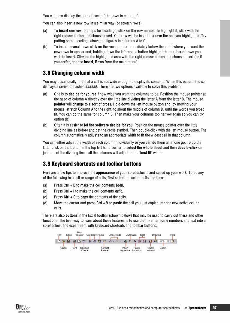
Part C Business mathematics and computer spreadsheets 5: Spreadsheets 97
You can now display the sum of each of the rows in column C.
You can also insert a new row in a similar way (or stretch rows).
(a) To insert one row, perhaps for headings, click on the row number to highlight it, click with the right mouse button and choose insert. One row will be inserted above the one you highlighted. Try putting some headings above the figures in columns A to C.
(b) To insert several rows click on the row number immediately below the point where you want the new rows to appear and, holding down the left mouse button highlight the number of rows you wish to insert. Click on the highlighted area with the right mouse button and choose Insert (or if you prefer, choose Insert, Rows from the main menu).
3.8 Changing column width You may occasionally find that a cell is not wide enough to display its contents. When this occurs, the cell displays a series of hashes ######. There are two options available to solve this problem.
(a) One is to decide for yourself how wide you want the columns to be. Position the mouse pointer at the head of column A directly over the little line dividing the letter A from the letter B. The mouse pointer will change to a sort of cross. Hold down the left mouse button and, by moving your mouse, stretch Column A to the right, to about the middle of column D, until the words you typed fit. You can do the same for column B. Then make your columns too narrow again so you can try option (b).
(b) Often it is easier to let the software decide for you. Position the mouse pointer over the little dividing line as before and get the cross symbol. Then double-click with the left mouse button. The column automatically adjusts to an appropriate width to fit the widest cell in that column.
You can either adjust the width of each column individually or you can do them all in one go. To do the latter click on the button in the top left hand corner to select the whole sheet and then double-click onjust one of the dividing lines: all the columns will adjust to the 'best fit' width.
3.9 Keyboard shortcuts and toolbar buttons Here are a few tips to improve the appearance of your spreadsheets and speed up your work. To do any of the following to a cell or range of cells, first select the cell or cells and then:
(a) Press Ctrl + B to make the cell contents bold.(b) Press Ctrl + I to make the cell contents italic.(c) Press Ctrl + C to copy the contents of the cells. (d) Move the cursor and press Ctrl + V to paste the cell you just copied into the new active cell or
cells.
There are also buttons in the Excel toolbar (shown below) that may be used to carry out these and other functions. The best way to learn about these features is to use them - enter some numbers and text into a spreadsheet and experiment with keyboard shortcuts and toolbar buttons.

98 5: Spreadsheets Part C Business mathematics and computer spreadsheets
4 Spreadsheet construction
A wide range of formulae and functions are available within Excel.
Spreadsheet models that will be used mainly as a calculation tool for various scenarios should ideally beconstructed in three sections, as follows.
1 An inputs section containing the variables (eg the amount of a loan and the interest rate). 2 A calculations section containing formulae (eg the loan term and interest rate).
Example: spreadsheet construction
In practice, in many situations it is often more convenient to combine the results and calculations areas as follows.
If we took out another loan of $4,789 at an interest rate of 7.25% we would simply need to overwrite the figures in the variable section of the spreadsheet with the new figures to calculate the interest.
FAST FORWARD
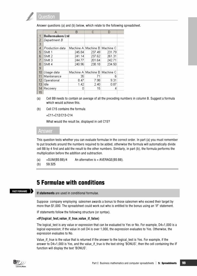
Part C Business mathematics and computer spreadsheets 5: Spreadsheets 99
QuestionAnswer questions (a) and (b) below, which relate to the following spreadsheet.
(a) Cell B9 needs to contain an average of all the preceding numbers in column B. Suggest a formula which would achieve this.
(b) Cell C15 contains the formula
=C11+C12/C13-C14
What would the result be, displayed in cell C15?
AnswerThis question tests whether you can evaluate formulae in the correct order. In part (a) you must remember to put brackets around the numbers required to be added, otherwise the formula will automatically divide cell B8 by 4 first and add the result to the other numbers. Similarly, in part (b), the formula performs the multiplication before the addition and subtraction.
(a) =SUM(B5:B8)/4 An alternative is = AVERAGE(B5:B8). (b) 59.325
5 Formulae with conditions
If statements are used in conditional formulae.
Suppose company employing salesmen awards a bonus to those salesmen who exceed their target by more than $1,000. The spreadsheet could work out who is entitled to the bonus using an ‘IF’ statement.
IF statements follow the following structure (or syntax).
=IF(logical_test,value_if_true,value_if_false)
The logical_test is any value or expression that can be evaluated to Yes or No. For example, D4>1,000 is a logical expression; if the value in cell D4 is over 1,000, the expression evaluates to Yes. Otherwise, the expression evaluates to No.
Value_if_true is the value that is returned if the answer to the logical_test is Yes. For example, if the answer to D4>1,000 is Yes, and the value_if_true is the text string "BONUS", then the cell containing the IF function will display the text "BONUS".
FAST FORWARD
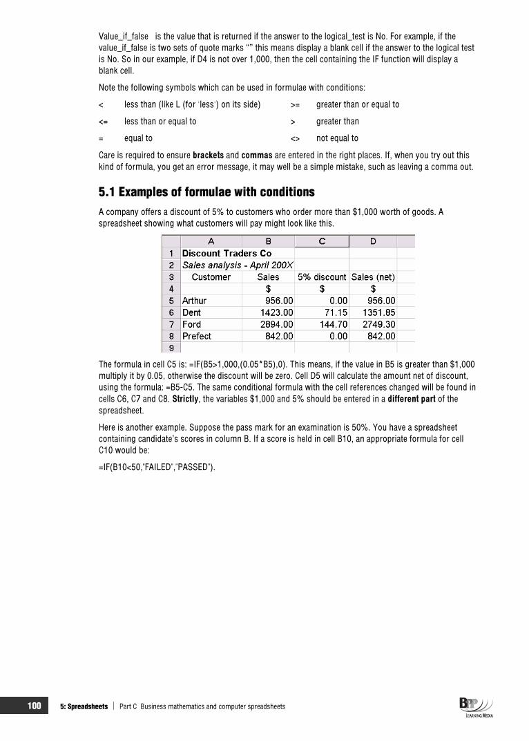
100 5: Spreadsheets Part C Business mathematics and computer spreadsheets
Value_if_false is the value that is returned if the answer to the logical_test is No. For example, if the value_if_false is two sets of quote marks “” this means display a blank cell if the answer to the logical test is No. So in our example, if D4 is not over 1,000, then the cell containing the IF function will display a blank cell.
Note the following symbols which can be used in formulae with conditions:
< less than (like L (for 'less') on its side) >= greater than or equal to
<= less than or equal to > greater than
= equal to <> not equal to
Care is required to ensure brackets and commas are entered in the right places. If, when you try out this kind of formula, you get an error message, it may well be a simple mistake, such as leaving a comma out.
5.1 Examples of formulae with conditions A company offers a discount of 5% to customers who order more than $1,000 worth of goods. A spreadsheet showing what customers will pay might look like this.
The formula in cell C5 is: =IF(B5>1,000,(0.05*B5),0). This means, if the value in B5 is greater than $1,000 multiply it by 0.05, otherwise the discount will be zero. Cell D5 will calculate the amount net of discount, using the formula: =B5-C5. The same conditional formula with the cell references changed will be found in cells C6, C7 and C8. Strictly, the variables $1,000 and 5% should be entered in a different part of the spreadsheet.
Here is another example. Suppose the pass mark for an examination is 50%. You have a spreadsheet containing candidate’s scores in column B. If a score is held in cell B10, an appropriate formula for cell C10 would be:
=IF(B10<50,"FAILED","PASSED").

Part C Business mathematics and computer spreadsheets 5: Spreadsheets 101
6 Charts and graphs
Excel includes the facility to produce a range of charts and graphs. The chart wizard provides a tool to simplify the process of chart construction.
Using Microsoft Excel, It is possible to display data held in a range of spreadsheet cells in a variety of charts or graphs. We will use the Discount Traders Co spreadsheet shown below to generate a chart.
The data in the spreadsheet could be used to generate a chart, such as those shown below. We explain how later in this section.
The Chart Wizard may also be used to generate a line graph. A line graph would normally be used to track a trend over time. For example, the chart below graphs the Total Revenue figures shown in Row 7 of the following spreadsheet.
FAST FORWARD

102 5: Spreadsheets Part C Business mathematics and computer spreadsheets
7 Spreadsheet format and appearance Good presentation can help people understand the contents of a spreadsheet.
7.1 Titles and labels A spreadsheet should be headed up with a title which clearly defines its purpose. Examples of titles are follows.
(a) Income statement for the year ended 30 June 200X.
(b) (i) Area A: Sales forecast for the three months to 31 March 200X. (ii) Area B: Sales forecast for the three months to 31 March 200X. (iii) Combined sales forecast for the three months to 31 March 200X.
(c) Salesmen: Analysis of earnings and commission for the six months ended 30 June 200X.
Row and column headings (or labels) should clearly identify the contents of the row/column. Any assumptions made that have influenced the spreadsheet contents should be clearly stated.
FAST FORWARD

Part C Business mathematics and computer spreadsheets 5: Spreadsheets 103
7.2 Formatting There are a wide range of options available under the Format menu. Some of these functions may also be accessed through toolbar buttons. Formatting options include the ability to:
(a) Add shading or borders to cells. (b) Use different sizes of text and different fonts.(c) Choose from a range of options for presenting values, for example to present a number as a
percentage (eg 0.05 as 5%), or with commas every third digit, or to a specified number of decimalplaces etc.
Experiment with the various formatting options yourself.
7.2.1 Formatting numbers
Most spreadsheet programs contain facilities for presenting numbers in a particular way. In Excel you simply click on Format and then Cells …to reach these options.
(a) Fixed format displays the number in the cell rounded off to the number of decimal places you select.
(b) Currency format displays the number with a '$' in front, with commas and not more than two decimal places, eg $10,540.23.
(c) Comma format is the same as currency format except that the numbers are displayed without the '$'.
(d) General format is the format assumed unless another format is specified. In general format the number is displayed with no commas and with as many decimal places as entered or calculated that fit in the cell.
(e) Percent format multiplies the number in the display by 100 and follows it with a percentage sign. For example the number 0.548 in a cell would be displayed as 54.8%.
(f) Hidden format is a facility by which values can be entered into cells and used in calculations but are not actually displayed on the spreadsheet. The format is useful for hiding sensitive information.
7.3 Gridlines One of the options available under the Tools, Options menu, on the View tab, is an option to remove the gridlines from your spreadsheet.
Compare the following two versions of the same spreadsheet. Note how the formatting applied to the second version has improved the spreadsheet presentation.

104 5: Spreadsheets Part C Business mathematics and computer spreadsheets
8 Other issues
Backing up is a key security measure. Cell protection and passwords can also be used to prevent unauthorised access.
8.1 Printing spreadsheets The print options for your spreadsheet may be accessed by selecting File and then Page Setup. The various Tabs contain a range of options. You specify the area of the spreadsheet to be printed in the Print area box on the Sheet tab. Other options include the ability to repeat headings on all pages and the option to print gridlines if required (normally they wouldn’t be!)
Experiment with these options including the options available under Header/Footer.
8.2 Controls There are facilities available in spreadsheet packages which can be used as controls – to prevent unauthorised or accidental amendment or deletion of all or part of a spreadsheet.
(a) Saving and back-up. When working on a spreadsheet, save your file regularly, as often as every ten minutes. This will prevent too much work being lost in the advent of a system crash. Spreadsheet files should be included in standard back-up procedures.
FAST FORWARD

Part C Business mathematics and computer spreadsheets 5: Spreadsheets 105
(b) Cell protection. This prevents the user from inadvertently changing or erasing cells that should not be changed. Look up how to protect cells using Excel's Help facility. (Select Help from the main menu within Excel, then select Contents and Index, click on the Find tab and enter the words 'cellprotection'.)
(c) Passwords. You can set a password for any spreadsheet that you create. In Excel, simply click on Tools, then on Protection, then on Protect Sheet or Protect Workbook, as appropriate.
8.3 Using spreadsheets with word processing software There may be a situation where you wish to incorporate the contents of all or part of a spreadsheet into a word processed report. There are a number of options available to achieve this.
(a) The simplest, but least professional option, is to print out the spreadsheet and interleave the page or pages at the appropriate point in your word processed document.
(b) A neater option if you are just including a small table is to select and copy the relevant cells from the spreadsheet to the computer's clipboard by selecting the cells and choosing Edit, Copy. Then switch to the word processing document, and paste them in at the appropriate point.
(c) Office packages, such as Microsoft Office allow you to easily use spreadsheets and word processing files together.
For example, a new, blank spreadsheet can be 'embedded' in a document by selecting Insert, Object then, from within the Create New tab, selecting Microsoft Excel worksheet. The spreadsheet is then available to be worked upon, allowing the easy manipulation of numbers using all the facilities of the spreadsheet package. Clicking outside the spreadsheet will result in the spreadsheet being inserted in the document.
The contents of an existing spreadsheet may be inserted into a Word document by choosing Insert, Object and then activating the Create from File tab. Then click the Browse button and locate the spreadsheet file. Highlight the file, then click Insert, and then OK. You may then need to move and resize the object, by dragging its borders, to fit your document.
9 Three dimensional (multi-sheet) spreadsheets
Spreadsheet packages permit the user to work with multiple sheets that refer to each other.
9.1 Background In early spreadsheet packages, a spreadsheet file consisted of a single worksheet. Excel provides the option of multi-sheet spreadsheets, consisting of a series of related sheets. Excel files which contain more than one worksheet are often called workbooks.
For example, suppose you were producing a profit forecast for two regions, and a combined forecast for the total of the regions. This situation would be suited to using separate worksheets for each region and another for the total. This approach is sometimes referred to as working in three dimensions, as you are able to flip between different sheets stacked in front or behind each other. Cells in one sheet may refer tocells in another sheet. So, in our example, the formulae in the cells in the total sheet would refer to the cells in the other sheets.
Excel has a series of 'tabs', one for each worksheet at the foot of the spreadsheet.
9.2 How many sheets? Excel can be set up so that it always opens a fresh file with a certain number of worksheets ready and waiting for you. Click on Tools … Options … and then the General tab and set the number Sheets in new workbook option to the number you would like each new spreadsheet file to contain (sheets may be added or deleted later).
FAST FORWARD
106 5: Spreadsheets Part C Business mathematics and computer spreadsheets
If you subsequently want to insert more sheets you just right click on the index tab after which you want the new sheet to be inserted and choose Insert … and then Worksheet. By default sheets are called Sheet1, Sheet 2 etc. However, these may be changed. To rename a sheet in Excel, right click on its index tab and choose the rename option.
9.3 Pasting from one sheet to another When building a spreadsheet that will contain a number of worksheets with identical structure, users often set up one sheet, then copy that sheet and amend the sheet contents. [To copy a worksheet in Excel, from within the worksheet you wish to copy, select Edit, Move or Copy sheet, and tick the Create a copy box.] A 'Total' sheet would use the same structure, but would contain formulae totalling the individual sheets.
9.4 Linking sheets with formulae Formulae on one sheet may refer to data held on another sheet. The links within such a formula may be established using the following steps.
Step 1 In the cell that you want to refer to a cell from another sheet, type =.
Step 2 Click on the index tab for the sheet containing the cell you want to refer to and select the cell in question.
Step 3 Press Enter or Return.
9.5 Uses for multi-sheet spreadsheets There are a wide range of situations suited to the multi-sheet approach. A variety of possible uses follow.
(a) A model could use one sheet for variables, a second for calculations, and a third for outputs. (b) To enable quick and easy consolidation of similar sets of data, for example the financial results of
two subsidiaries or the budgets of two departments. (c) To provide different views of the same data. For instance you could have one sheet of data sorted
in product code order and another sorted in product name order.
10 Macros
A macro is an automated process that may be written by recording key-strokes and mouse clicks.
If you perform a task repeatedly within a spreadsheet, you may want to make your life easier by automating the task. This is what macros are used for.
A macro is a series of commands or functions that are stored in your spreadsheet and can be run each time you want to perform the task.
One example would be the frequent use of long strings of text in formulae. By creating a macro, you can format the cells to which the formula will apply, rather than having to type in the formula each time.
When you record a macro, your spreadsheet package should store information about each step you take as you perform a series of commands. You can then run the macro to repeat the commands. This allows you to check for any errors.
10.1 Working with macros Always start a macro by returning the cursor to cell A1 (by pressing Ctrl + Home), even if it is already there. You may well not want to make your first entry in cell A1, but if you select your first real cell (B4 say) before you start recording, the macro will always begin at the currently active cell, whether it is B4 or Z256.
Always finish a macro by selecting the cell where the next entry is required.
FAST FORWARD

Part C Business mathematics and computer spreadsheets 5: Spreadsheets 107
If you close down and then re-open the file in which you created the macro, your macro will work again, because it is actually stored in that file. If you want your macro to be available to you whenever you want it you have the following choices.
(a) Keep this file, with no contents other than your 'name' macro (and any others you may write) and always use it as the basis for any new spreadsheets you create, which will subsequently be saved with new file names.
(b) You can add the macro to your Personal Macro Workbook. You do this at the point when you are naming your workbook and choosing a shortcut key, by changing the option in the Store macro in: box from This Workbook to Personal Macro Workbook. The macro will then be loaded into memory whenever you start up Excel and be available in any spreadsheet you create.
If you forget to assign a keyboard shortcut to a macro (or do not want to do so), you can still run your macros by clicking on Tools …Macro … Macros. This gives you a list of all the macros currently available. Select the one you want then click on Run.
Do not accept the default names offered by Excel of Macro1, Macro2 etc. You will soon forget what these macros do, unless you give them a meaningful name.
11 Advantages and disadvantages of spreadsheet software
11.1 Advantages of spreadsheets Excel is easy to learn and to use Spreadsheets make the calculation and manipulation of data easier and quicker They enable the analysis, reporting and sharing of financial information They enable ‘what-if’ analysis to be performed very quickly
11.2 Disadvantages of spreadsheets A spreadsheet is only as good as its original design, garbage in = garbage out! Formulae are hidden from sight so the underlying logic of a set of calculations may not be obvious A spreadsheet presentation may make reports appear infallible Research shows that a high proportion of large models contain critical errors A database may be more suitable to use with large volumes of data
Question Spreadsheet advantages
An advantage of a spreadsheet program is that it
A Can answer 'what if?' questions B Checks for incorrect entries C Automatically writes formulae D Can answer 'when is?' questions
AnswerThe correct answer is A.

108 5: Spreadsheets Part C Business mathematics and computer spreadsheets
12 Uses of spreadsheet software Spreadsheets can be used in a variety of accounting contexts. You should practise using spreadsheets, hands-on experience is the key to spreadsheet proficiency.
Management accountants will use spreadsheet software in activities such as budgeting, forecasting, reporting performance and variance analysis.
12.1 Budgeting Spreadsheet packages for budgeting have a number of advantages.
(a) Spreadsheet packages have a facility to perform 'what if' calculations at great speed. For example, the consequences throughout the organisation of sales growth per month of nil, 1/2%, 1%, 11/2%and so on can be calculated very quickly.
(b) Preparing budgets may be complex; budgets may need to go through several drafts. If one or two figures are changed, the computer will automatically make all the computational changes to the other figures.
(c) A spreadsheet model will ensure that the preparation of the individual budgets is co-ordinated.Data and information from the production budget, for example, will be automatically fed through to the material usage budget (as material usage will depend on production levels).
These advantages of spreadsheets make them ideal for taking over the manipulation of numbers, leaving staff to get involved in the real planning process.
FAST FORWARD

Part C Business mathematics and computer spreadsheets 5: Spreadsheets 109
Chapter Roundup
Use of spreadsheets is an essential part of the day-to-day work of the Management Accountant.
A spreadsheet is an electronic piece of paper divided into rows and columns. The intersection of a row and a column is known as a cell.
Formulas in Microsoft Excel follow a specific syntax.
Essential basic skills include how to move around within a spreadsheet, how to enter and edit data, how to fill cells, how to insert and delete columns and rows and how to improve the basic layout andappearance of a spreadsheet.
A wide range of formulae and functions are available within Excel.
If statements are used in conditional formulae.
Excel includes the facility to produce a range of charts and graphs. The chart wizard provides a tool to simplify the process of chart construction.
Good presentation can help people understand the contents of a spreadsheet.
Backing up is a key security measure. Cell protection and passwords can also be used to prevent unauthorised access.
Spreadsheet packages permit the user to work with multiple sheets that refer to each other.
A macro is an automated process that may be written by recording key-strokes and mouse clicks.
Spreadsheets can be used in a variety of accounting contexts. You should practise using spreadsheets, hands-on experience is the key to spreadsheet proficiency.
Quick quiz 1 List three types of cell contents. 2 What do the F5 and F2 keys do in Excel? 3 What technique can you use to insert a logical series of data such as 1, 2 …. 10, or Jan, Feb, March etc? 4 How do you display formulae instead of the results of formulae in a spreadsheet? 5 Which function key may be used to change cell references within a selected formula from absolute to
relative – and vice-versa? 6 List five possible changes that may improve the appearance of a spreadsheet. 7 List three possible uses for a multi-sheet (3D) spreadsheet. 8 You are about to key an exam mark into cell B4 of a spreadsheet. Write an IF statement, to be placed in
cell C4, that will display PASS in C4 if the student mark is 50 or above - and or will display FAIL if the mark is below 50 (all student marks are whole numbers).
9 Give two ways of starting Excel's function wizard.

110 5: Spreadsheets Part C Business mathematics and computer spreadsheets
Answers to quick quiz 1 Text, values or formulae. 2 F5 opens a GoTo dialogue box which is useful for navigating around large spreadsheets. F2 puts the active
cell into edit mode. 3 You can use the technique of 'filling' - selecting the first few items of a series and dragging the lower right
corner of the selection in the appropriate direction. 4 Select Tools, Options, ensure the View tab is active then tick the Formulas box within the window options
area.5 The F4 key. 6 Removing gridlines, adding shading, adding borders, using different fonts and font sizes, presenting
numbers as percentages or currency or to a certain number of decimal places. 7 The construction of a spreadsheet model with separate Input, Calculation and Output sheets. They can
help consolidate data from different sources. They can offer different views of the same data. 8 =IF(A4>49,"PASS","FAIL ") 9 You could click on the fx symbol in the toolbar, or use the menu item Insert, Function, to start the function
wizard.
Now try the questions below from the Exam Question Bank
Number Level Marks Time
5 MCQ/OTQ n/a n/a

111
Cost accounting techniques
P
A
R
T
D

112

113
Material costs
IntroductionThe investment in inventory is a very important one for most businesses, both in terms of monetary value and relationships with customers (no inventory, no sale, loss of customer goodwill). It is therefore vital that management establish and maintain an effective inventory control system.
This chapter will concentrate on a inventory control system for materials, but similar problems and considerations apply to all forms of inventory.
Topic list Syllabus reference
1 What is inventory control? D1 (b)
2 The ordering, receipt and issue of raw materials D1 (a)
3 The storage of raw materials D1 (c), (d)
4 Inventory control levels D1 (e)-(h)
5 Accounting for material costs D1(c)
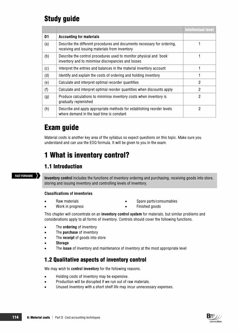
114 6: Material costs Part D Cost accounting techniques
Study guide Intellectual level
D1 Accounting for materials
(a) Describe the different procedures and documents necessary for ordering, receiving and issuing materials from inventory
1
(b) Describe the control procedures used to monitor physical and 'book' inventory and to minimise discrepancies and losses
1
(c) Interpret the entries and balances in the material inventory account 1
(d) Identify and explain the costs of ordering and holding inventory 1
(e) Calculate and interpret optimal recorder quantities 2
(f) Calculate and interpret optimal reorder quantities when discounts apply 2
(g) Produce calculations to minimise inventory costs when inventory is gradually replenished
2
(h) Describe and apply appropriate methods for establishing reorder levels where demand in the lead time is constant
2
Exam guide Material costs is another key area of the syllabus so expect questions on this topic. Make sure you understand and can use the EOQ formula. It will be given to you in the exam.
1 What is inventory control? 1.1 Introduction
Inventory control includes the functions of inventory ordering and purchasing, receiving goods into store, storing and issuing inventory and controlling levels of inventory.
Classifications of inventories
Raw materials Spare parts/consumables Work in progress Finished goods
This chapter will concentrate on an inventory control system for materials, but similar problems and considerations apply to all forms of inventory. Controls should cover the following functions.
The ordering of inventory The purchase of inventory The receipt of goods into store
Storage The issue of inventory and maintenance of inventory at the most appropriate level
1.2 Qualitative aspects of inventory control We may wish to control inventory for the following reasons.
Holding costs of inventory may be expensive. Production will be disrupted if we run out of raw materials. Unused inventory with a short shelf life may incur unnecessary expenses.
FAST FORWARD

Part D Cost accounting techniques 6: Material costs 115
If manufactured goods are made out of low quality materials, the end product will be of low quality also. It may therefore be necessary to control the quality of inventory, in order to maintain a good reputation with consumers.
2 The ordering, receipt and issue of raw materials 2.1 Ordering and receiving materials
Every movement of a material in a business should be documented using the following as appropriate: purchase requisition; purchase order; GRN; materials requisition note; materials transfer note and materials returned note.
Proper records must be kept of the physical procedures for ordering and receiving a consignment of materials to ensure the following.
That enough inventory is held That there is no duplication of ordering That quality is maintained That there is adequate record keeping for accounts purposes
2.2 Purchase requisition Current inventories run down to the level where a reorder is required. The stores department issues a purchase requisition which is sent to the purchasing department, authorising the department to order further inventory. An example of a purchase requisition is shown below.
2.3 Purchase order The purchasing department draws up a purchase order which is sent to the supplier. (The supplier may be asked to return an acknowledgement copy as confirmation of his acceptance of the order.) Copies of the purchase order must be sent to the accounts department and the storekeeper (or receiving department).
FAST FORWARD
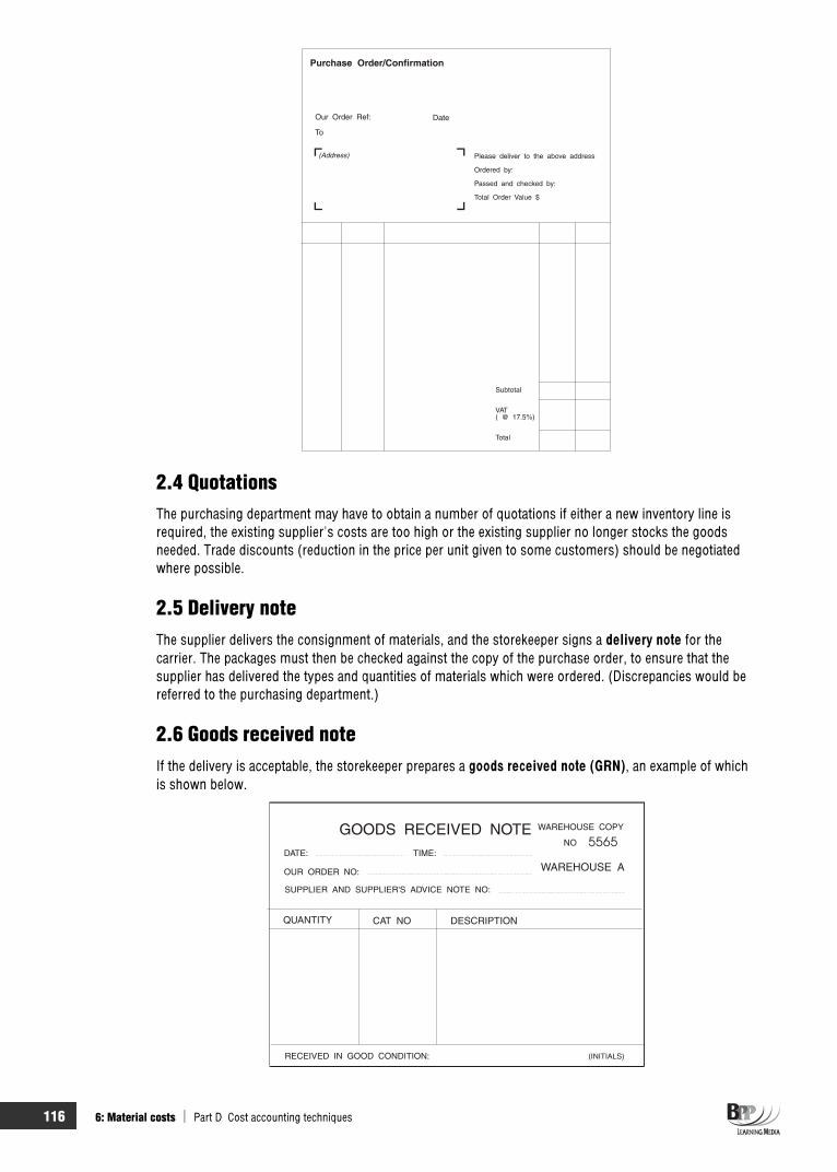
116 6: Material costs Part D Cost accounting techniques
2.4 Quotations The purchasing department may have to obtain a number of quotations if either a new inventory line is required, the existing supplier's costs are too high or the existing supplier no longer stocks the goods needed. Trade discounts (reduction in the price per unit given to some customers) should be negotiated where possible.
2.5 Delivery note The supplier delivers the consignment of materials, and the storekeeper signs a delivery note for the carrier. The packages must then be checked against the copy of the purchase order, to ensure that the supplier has delivered the types and quantities of materials which were ordered. (Discrepancies would be referred to the purchasing department.)
2.6 Goods received note If the delivery is acceptable, the storekeeper prepares a goods received note (GRN), an example of which is shown below.

Part D Cost accounting techniques 6: Material costs 117
A copy of the GRN is sent to the accounts department, where it is matched with the copy of the purchase order. The supplier's invoice is checked against the purchase order and GRN, and the necessary steps are taken to pay the supplier. The invoice may contain details relating to discounts such as trade discounts, quantity discounts (order in excess of a specified amount) and settlement discounts (payment received within a specified number of days).
Question Ordering materials
What are the possible consequences of a failure of control over ordering and receipt of materials?
Answer(a) Incorrect materials being delivered, disrupting operations (b) Incorrect prices being paid (c) Deliveries other than at the specified time (causing disruption) (d) Insufficient control over quality (e) Invoiced amounts differing from quantities of goods actually received or prices agreed
You may, of course, have thought of equally valid consequences.
2.7 Materials requisition note Materials can only be issued against a materials/stores requisition. This document must record not only the quantity of goods issued, but also the cost centre or the job number for which the requisition is being made. The materials requisition note may also have a column, to be filled in by the cost department, for recording the cost or value of the materials issued to the cost centre or job.
2.8 Materials transfers and returns Where materials, having been issued to one job or cost centre, are later transferred to a different job or cost centre, without first being returned to stores, a materials transfer note should be raised. Such a note must show not only the job receiving the transfer, but also the job from which it is transferred. This enables the appropriate charges to be made to jobs or cost centres.
Material returns must also be documented on a materials returned note. This document is the 'reverse' of a requisition note, and must contain similar information. In fact it will often be almost identical to a requisition note. It will simply have a different title and perhaps be a distinctive colour, such as red, to highlight the fact that materials are being returned.

118 6: Material costs Part D Cost accounting techniques
2.9 Computerised inventory control systems Many inventory control systems these days are computerised. Computerised inventory control systems vary greatly, but most will have the features outlined below.
(a) Data must be input into the system. For example, details of goods received may simply be written on to a GRN for later entry into the computer system. Alternatively, this information may be keyed in directly to the computer: a GRN will be printed and then signed as evidence of the transaction, so that both the warehouse and the supplier can have a hard copy record in case of dispute. Some systems may incorporate the use of devices such as bar code readers.
Other types of transaction which will need to be recorded include the following.
(i) Transfers between different categories of inventory (for example from work in progress to finished goods)
(ii) Despatch, resulting from a sale, of items of finished goods to customers (iii) Adjustments to inventory records if the amount of inventory revealed in a physical inventory
count differs from the amount appearing on the inventory records
(b) An inventory master file is maintained. This file will contain details for every category of inventory and will be updated for new inventory lines. A database file may be maintained.
Question Inventory master file
What type of information do you think should be held on an inventory master file?
AnswerHere are some examples.
(a) Inventory code number, for reference (e) Cost per unit (b) Brief description of inventory item (f) Selling price per unit (if finished goods) (c) Reorder level (g) Amount in inventory (d) Reorder quantity (h) Frequency of usage
The file may also hold details of inventory movements over a period, but this will depend on the type of system in operation. In a batch system, transactions will be grouped and input in one operation and details of the movements may be held in a separate transactions file, the master file updated in total only. In an on-line system, transactions may be input directly to the master file, where the record of movements is thus likely to be found. Such a system will mean that the inventory records are constantly up to date, which will help in monitoring and controlling inventory.
The system may generate orders automatically once the amount in inventory has fallen to the reorder level.
(c) The system will generate outputs. These may include, depending on the type of system, any of the following.
(i) Hard copy records, for example a printed GRN, of transactions entered into the system. (ii) Output on a VDU screen in response to an enquiry (for example the current level of a
particular line of inventory, or details of a particular transaction). (iii) Various printed reports, devised to fit in with the needs of the organisation. These may
include inventory movement reports, detailing over a period the movements on all inventory lines, listings of GRNs, despatch notes and so forth.
A computerised inventory control system is usually able to give more up to date information and more flexible reporting than a manual system but remember that both manual and computer based inventory control systems need the same types of data to function properly.

Part D Cost accounting techniques 6: Material costs 119
3 The storage of raw materials 3.1 Objectives of storing materials Speedy issue and receipt of materials Full identification of all materials at all times Correct location of all materials at all times
Protection of materials from damage and deterioration Provision of secure stores to avoid pilferage, theft and fire
Efficient use of storage space Maintenance of correct inventory levels
Keeping correct and up-to-date records of receipts, issues and inventory levels
3.2 Recording inventory levels One of the objectives of storekeeping is to maintain accurate records of current inventory levels. This involves the accurate recording of inventory movements (issues from and receipts into stores). The most frequently encountered system for recording inventory movements is the use of bin cards and stores ledger accounts.
3.2.1 Bin cards
A bin card shows the level of inventory of an item at a particular stores location. It is kept with the actual inventory and is updated by the storekeeper as inventories are received and issued. A typical bin card is shown below.
The use of bin cards is decreasing, partly due to the difficulty in keeping them updated and partly due to the merging of inventory recording and control procedures, frequently using computers.
3.2.2 Stores ledger accounts
A typical stores ledger account is shown below. Note that it shows the value of inventory.
The above illustration shows a card for a manual system, but even when the inventory records are computerised, the same type of information is normally included in the computer file. The running balance on the stores ledger account allows inventory levels and valuation to be monitored.

120 6: Material costs Part D Cost accounting techniques
3.2.3 Free inventory
Managers need to know the free inventory balance in order to obtain a full picture of the current inventory position of an item. Free inventory represents what is really available for future use and is calculated as follows.
Materials in inventory X+ Materials on order from suppliers X– Materials requisitioned, not yet issued (X) Free inventory balance X
Knowledge of the level of physical inventory assists inventory issuing, inventory counting and controlling maximum and minimum inventory levels: knowledge of the level of free inventory assists ordering.
Question Units on order
A wholesaler has 8,450 units outstanding for Part X100 on existing customers' orders; there are 3,925 units in inventory and the calculated free inventory is 5,525 units.
How many units does the wholesaler have on order with his supplier?
A 9,450 B 10,050 C 13,975 D 17,900
AnswerFree inventory balance = units in inventory + units on order – units ordered, but not yet issued
5,525 = 3,925 + units on order – 8,450 Units on order = 10,050
The correct answer is B.
3.3 Identification of materials: inventory codes (materials codes) Materials held in stores are coded and classified. Advantages of using code numbers to identify materials are as follows.
(a) Ambiguity is avoided. (b) Time is saved. Descriptions can be lengthy and time-consuming. (c) Production efficiency is improved. The correct material can be accurately identified from a code
number.(d) Computerised processing is made easier. (e) Numbered code systems can be designed to be flexible, and can be expanded to include more
inventory items as necessary.
The digits in a code can stand for the type of inventory, supplier, department and so forth.
3.4 The inventory count (stocktake)
The inventory count (stocktake) involves counting the physical inventory on hand at a certain date, and then checking this against the balance shown in the inventory records. The count can be carried out on a continuous or periodic basis.
FAST FORWARD

Part D Cost accounting techniques 6: Material costs 121
Periodic stocktaking is a process whereby all inventory items are physically counted and valued at a set point in time, usually at the end of an accounting period.
Continuous stocktaking is counting and valuing selected items at different times on a rotating basis. This involves a specialist team counting and checking a number of inventory items each day, so that each item is checked at least once a year. Valuable items or items with a high turnover could be checked more frequently.
3.4.1 Advantages of continuous stocktaking compared to periodic stocktaking
(a) The annual stocktaking is unnecessary and the disruption it causes is avoided. (b) Regular skilled stocktakers can be employed, reducing likely errors. (c) More time is available, reducing errors and allowing investigation. (d) Deficiencies and losses are revealed sooner than they would be if stocktaking were limited to an
annual check. (e) Production hold-ups are eliminated because the stores staff are at no time so busy as to be unable
to deal with material issues to production departments. (f) Staff morale is improved and standards raised. (g) Control over inventory levels is improved, and there is less likelihood of overstocking or running
out of inventory.
3.4.2 Inventory discrepancies
There will be occasions when inventory checks disclose discrepancies between the physical amount of an item in inventory and the amount shown in the inventory records. When this occurs, the cause of the discrepancy should be investigated, and appropriate action taken to ensure that it does not happen again.
3.4.3 Perpetual inventory
Perpetual inventory refers to a inventory recording system whereby the records (bin cards and stores ledger accounts) are updated for each receipt and issue of inventory as it occurs.
This means that there is a continuous record of the balance of each item of inventory. The balance on the stores ledger account therefore represents the inventory on hand and this balance is used in the calculation of closing inventory in monthly and annual accounts. In practice, physical inventories may not agree with recorded inventories and therefore continuous stocktaking is necessary to ensure that the perpetual inventory system is functioning correctly and that minor inventory discrepancies are corrected.
3.4.4 Obsolete, deteriorating and slow-moving inventories and wastage
Obsolete inventories are those items which have become out-of-date and are no longer required. Obsolete items are written off and disposed of.
Inventory items may be wasted because, for example, they get broken. All wastage should be noted on the inventory records immediately so that physical inventory equals the inventory balance on records and the cost of the wastage written off.
Slow-moving inventories are inventory items which are likely to take a long time to be used up. For example, 5,000 units are in inventory, and only 20 are being used each year. This is often caused by overstocking. Managers should investigate such inventory items and, if it is felt that the usage rate is unlikely to increase, excess inventory should be written off as for obsolete inventory, leaving perhaps four or five years' supply in inventory.
Key terms
FAST FORWARD
FAST FORWARD

122 6: Material costs Part D Cost accounting techniques
4 Inventory control levels 4.1 Inventory costs
Inventory costs include purchase costs, holding costs, ordering costs and costs of running out inventory.
The costs of purchasing inventory are usually one of the largest costs faced by an organisation and, once obtained, inventory has to be carefully controlled and checked.
4.1.1 Reasons for holding inventories
To ensure sufficient goods are available to meet expected demand To provide a buffer between processes To meet any future shortages To take advantage of bulk purchasing discounts To absorb seasonal fluctuations and any variations in usage and demand To allow production processes to flow smoothly and efficiently As a necessary part of the production process (such as when maturing cheese) As a deliberate investment policy, especially in times of inflation or possible shortages
4.1.2 Holding costs
If inventories are too high, holding costs will be incurred unnecessarily. Such costs occur for a number of reasons.
(a) Costs of storage and stores operations. Larger inventories require more storage space and possibly extra staff and equipment to control and handle them.
(b) Interest charges. Holding inventories involves the tying up of capital (cash) on which interest must be paid.
(c) Insurance costs. The larger the value of inventories held, the greater insurance premiums are likely to be.
(d) Risk of obsolescence. The longer a inventory item is held, the greater is the risk of obsolescence. (e) Deterioration. When materials in store deteriorate to the extent that they are unusable, they must
be thrown away with the likelihood that disposal costs would be incurred.
4.1.3 Costs of obtaining inventory
On the other hand, if inventories are kept low, small quantities of inventory will have to be ordered more frequently, thereby increasing the following ordering or procurement costs.
(a) Clerical and administrative costs associated with purchasing, accounting for and receiving goods (b) Transport costs(c) Production run costs, for inventory which is manufactured internally rather than purchased from
external sources
4.1.4 Stockout costs (running out of inventory)
An additional type of cost which may arise if inventory are kept too low is the type associated with running out of inventory. There are a number of causes of stockout costs.
Lost contribution from lost sales Loss of future sales due to disgruntled customers Loss of customer goodwill Cost of production stoppages Labour frustration over stoppages Extra costs of urgent, small quantity, replenishment orders
FAST FORWARD

Part D Cost accounting techniques 6: Material costs 123
4.1.5 Objective of inventory control
The overall objective of inventory control is, therefore, to maintain inventory levels so that the total of the following costs is minimised.
Holding costs Stockout costs Ordering costs
4.2 Inventory control levels
Inventory control levels can be calculated in order to maintain inventories at the optimum level. The three critical control levels are reorder level, minimum level and maximum level.
Based on an analysis of past inventory usage and delivery times, inventory control levels can be calculated and used to maintain inventory at their optimum level (in other words, a level which minimises costs). These levels will determine 'when to order' and 'how many to order'.
4.2.1 Reorder level When inventories reach this level, an order should be placed to replenish inventories. The reorder level is determined by consideration of the following.
The maximum rate of consumption The maximum lead time
The maximum lead time is the time between placing an order with a supplier, and the inventory becoming available for use
Reorder level = maximum usage maximum lead time
4.2.2 Minimum level This is a warning level to draw management attention to the fact that inventories are approaching a dangerously low level and that stockouts are possible.
Minimum level = reorder level – (average usage average lead time)
4.2.3 Maximum level This also acts as a warning level to signal to management that inventories are reaching a potentially wasteful level.
Maximum level = reorder level + reorder quantity – (minimum usage minimum lead time)
Question Maximum inventory level
A large retailer with multiple outlets maintains a central warehouse from which the outlets are supplied. The following information is available for Part Number SF525.
Average usage 350 per day Minimum usage 180 per day Maximum usage 420 per day Lead time for replenishment 11-15 days Re-order quantity 6,500 units Re-order level 6,300 units
(a) Based on the data above, what is the maximum level of inventory?
A 5,250 B 6,500 C 10,820 D 12,800
Formula to learn
Formula to learn
Formula to learn
FAST FORWARD

124 6: Material costs Part D Cost accounting techniques
(b) Based on the data above, what is the approximate number of Part Number SF525 carried as buffer inventory?
A 200 B 720 C 1,680 D 1,750
Answer(a) Maximum inventory level = reorder level + reorder quantity – (min usage min lead time)
= 6,300 + 6,500 – (180 11) = 10,820
The correct answer is C.
Using good MCQ technique, if you were resorting to a guess you should have eliminated option A. The maximum inventory level cannot be less than the reorder quantity.
(b) Buffer inventory = minimum level
Minimum level = reorder level – (average usage average lead time) = 6,300 – (350 13) = 1,750.
The correct answer is D.
Option A could again be easily eliminated. With minimum usage of 180 per day, a buffer inventory of only 200 would not be much of a buffer!
4.2.4 Reorder quantity
This is the quantity of inventory which is to be ordered when inventory reaches the reorder level. If it is set so as to minimise the total costs associated with holding and ordering inventory, then it is known as the economic order quantity.
4.2.5 Average inventory
The formula for the average inventory level assumes that inventory levels fluctuate evenly between the minimum (or safety) inventory level and the highest possible inventory level (the amount of inventory immediately after an order is received, ie safety inventory + reorder quantity).
Average inventory = safety inventory + ½ reorder quantity
Question Average inventory
A component has a safety inventory of 500, a re-order quantity of 3,000 and a rate of demand which varies between 200 and 700 per week. The average inventory is approximately
A 2,000 B 2,300 C 2,500 D 3,500
AnswerAverage inventory = safety inventory + ½ reorder quantity
= 500 + (0.5 3,000) = 2,000
The correct answer is A.
Formula to learn
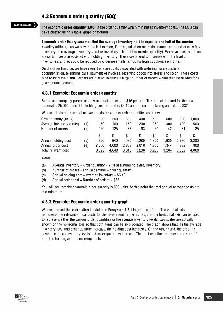
Part D Cost accounting techniques 6: Material costs 125
4.3 Economic order quantity (EOQ)
The economic order quantity (EOQ) is the order quantity which minimises inventory costs. The EOQ can be calculated using a table, graph or formula.
Economic order theory assumes that the average inventory held is equal to one half of the reorder quantity (although as we saw in the last section, if an organisation maintains some sort of buffer or safety inventory then average inventory = buffer inventory + half of the reorder quantity). We have seen that there are certain costs associated with holding inventory. These costs tend to increase with the level of inventories, and so could be reduced by ordering smaller amounts from suppliers each time.
On the other hand, as we have seen, there are costs associated with ordering from suppliers: documentation, telephone calls, payment of invoices, receiving goods into stores and so on. These costs tend to increase if small orders are placed, because a larger number of orders would then be needed for a given annual demand.
4.3.1 Example: Economic order quantity
Suppose a company purchases raw material at a cost of $16 per unit. The annual demand for the raw material is 25,000 units. The holding cost per unit is $6.40 and the cost of placing an order is $32.
We can tabulate the annual relevant costs for various order quantities as follows.
Order quantity (units) 100 200 300 400 500 600 800 1,000Average inventory (units) (a) 50 100 150 200 250 300 400 500Number of orders (b) 250 125 83 63 50 42 31 25
$ $ $ $ $ $ $ $Annual holding cost (c) 320 640 960 1,280 1,600 1,920 2,560 3,200Annual order cost (d) 8,000 4,000 2,656 2,016 1,600 1,344 992 800Total relevant cost 8,320 4,640 3,616 3,296 3,200 3,264 3,552 4,000
Notes
(a) Average inventory = Order quantity 2 (ie assuming no safety inventory) (b) Number of orders = annual demand order quantity (c) Annual holding cost = Average inventory $6.40 (d) Annual order cost = Number of orders $32
You will see that the economic order quantity is 500 units. At this point the total annual relevant costs are at a minimum.
4.3.2 Example: Economic order quantity graph
We can present the information tabulated in Paragraph 4.3.1 in graphical form. The vertical axis represents the relevant annual costs for the investment in inventories, and the horizontal axis can be used to represent either the various order quantities or the average inventory levels; two scales are actually shown on the horizontal axis so that both items can be incorporated. The graph shows that, as the average inventory level and order quantity increase, the holding cost increases. On the other hand, the ordering costs decline as inventory levels and order quantities increase. The total cost line represents the sum of both the holding and the ordering costs.
FAST FORWARD
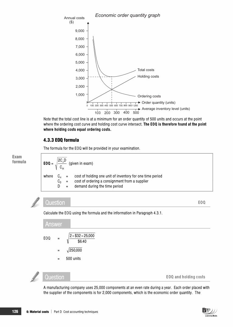
126 6: Material costs Part D Cost accounting techniques
Note that the total cost line is at a minimum for an order quantity of 500 units and occurs at the point where the ordering cost curve and holding cost curve intersect. The EOQ is therefore found at the point where holding costs equal ordering costs.
4.3.3 EOQ formula
The formula for the EOQ will be provided in your examination.
EOQ = HC
D2C0 (given in exam)
where CH = cost of holding one unit of inventory for one time period C0 = cost of ordering a consignment from a supplier D = demand during the time period
Question EOQ
Calculate the EOQ using the formula and the information in Paragraph 4.3.1.
Answer
EOQ = 40.6$
000,2532$2
= 000,250
= 500 units
Question EOQ and holding costs
A manufacturing company uses 25,000 components at an even rate during a year. Each order placed with the supplier of the components is for 2,000 components, which is the economic order quantity. The
Examformula

Part D Cost accounting techniques 6: Material costs 127
company holds a buffer inventory of 500 components. The annual cost of holding one component in inventory is $2.
What is the total annual cost of holding inventory of the component?
A $2,000 B $2,500 C $3,000 D $4,000
AnswerThe correct answer is C.
[Buffer inventory + (EOQ/2)] x Annual holding cost per component
= [500 + (2,000/2)] x $2
= $3,000
This question appeared in the June 2008 exam and was answered correctly by less than one third of candidates. A number of students chose choice D which is the EOQ x annual holding cost per component.Choice B was also popular (where the buffer stock is also divided by 2). Make sure you understand how to use the EOQ formula for different purposes such as this.
4.4 Economic batch quantity (EBQ)
The economic batch quantity (EBQ) is a modification of the EOQ and is used when resupply is gradual instead of instantaneous.
EBQ = D/R)(1C
D2C
H
0
Typically, a manufacturing company might hold inventories of a finished item, which is produced in batches. Once the order for a new batch has been placed, and the production run has started, finished output might be used before the batch run has been completed.
4.4.1 Example: Economic batch quantity
If the daily demand for an item of inventory is ten units, and the storekeeper orders 100 units in a batch. The rate of production is 50 units a day.
(a) On the first day of the batch production run, the stores will run out of its previous inventories, and re-supply will begin. 50 units will be produced during the day, and ten units will be consumed. The closing inventory at the end of day 1 will be 50 – 10 = 40 units.
(b) On day 2, the final 50 units will be produced and a further ten units will be consumed. Closing inventory at the end of day 2 will be (40 + 50 –10) = 80 units.
(c) In eight more days, inventories will fall to zero.
The minimum inventory in this example is zero, and the maximum inventory is 80 units. The maximum inventory is the quantity ordered (Q = 100) minus demand during the period of the batch production run which is Q D/R, where
D is the rate of demand R is the rate of production Q is the quantity ordered.
In our example, the maximum inventory is (100 – 5010
100) = 100 – 20 = 80 units.
The maximum inventory level, given gradual re-supply, is thus Q – R
QD = Q(1 – D/R).
FAST FORWARD
Exam focus point
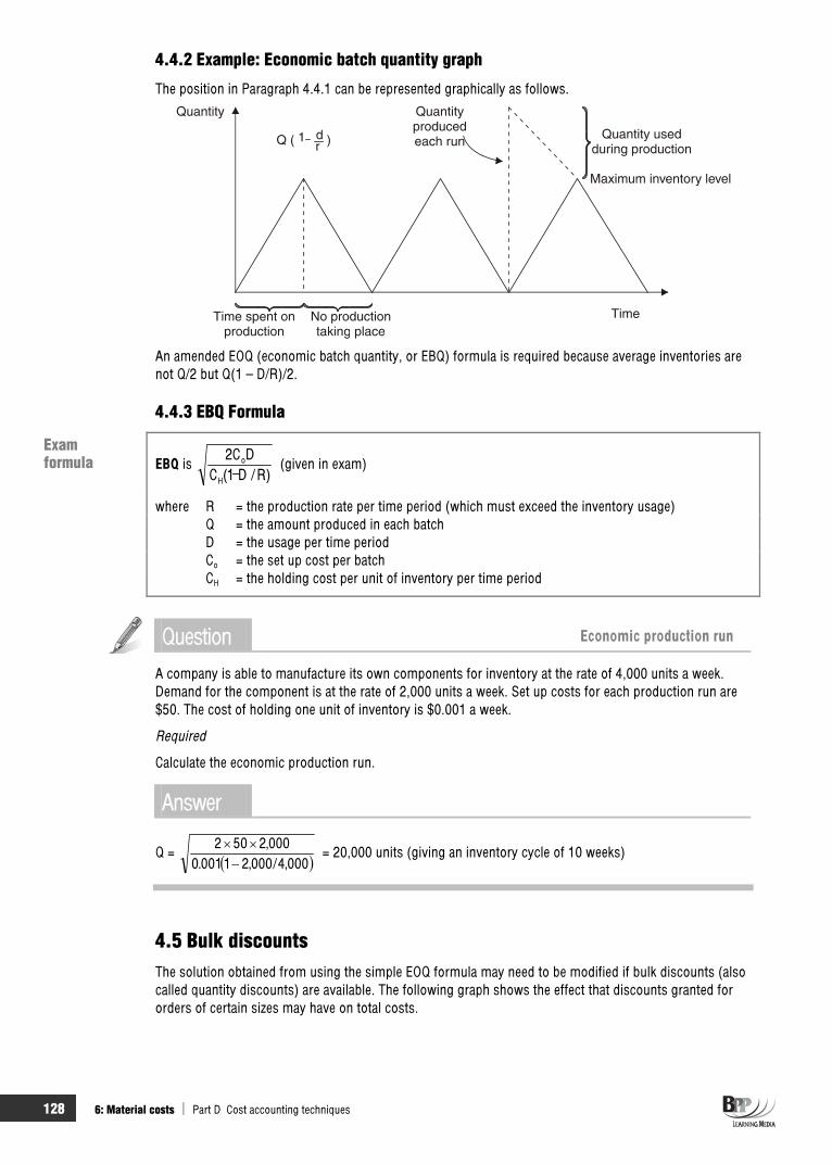
128 6: Material costs Part D Cost accounting techniques
4.4.2 Example: Economic batch quantity graph
The position in Paragraph 4.4.1 can be represented graphically as follows.
An amended EOQ (economic batch quantity, or EBQ) formula is required because average inventories are not Q/2 but Q(1 – D/R)/2.
4.4.3 EBQ Formula
EBQ is )R/D_1(C
DC2
H
o (given in exam)
where R = the production rate per time period (which must exceed the inventory usage) Q = the amount produced in each batch D = the usage per time period Co = the set up cost per batch CH = the holding cost per unit of inventory per time period
Question Economic production run
A company is able to manufacture its own components for inventory at the rate of 4,000 units a week. Demand for the component is at the rate of 2,000 units a week. Set up costs for each production run are $50. The cost of holding one unit of inventory is $0.001 a week.
Required
Calculate the economic production run.
Answer
Q = 000,4/000,21001.0
000,2502 = 20,000 units (giving an inventory cycle of 10 weeks)
4.5 Bulk discounts The solution obtained from using the simple EOQ formula may need to be modified if bulk discounts (also called quantity discounts) are available. The following graph shows the effect that discounts granted for orders of certain sizes may have on total costs.
Examformula

Part D Cost accounting techniques 6: Material costs 129
The graph above shows the following.
Differing bulk discounts are given when the order quantity exceeds A, B and C The minimum total cost (ie when quantity B is ordered rather than the EOQ)
To decide mathematically whether it would be worthwhile taking a discount and ordering larger quantities, it is necessary to minimise the total of the following.
Total material costs Inventory holding costs Ordering costs
The total cost will be minimised at one of the following.
At the pre-discount EOQ level, so that a discount is not worthwhile At the minimum order size necessary to earn the discount
4.5.1 Example: Bulk discounts
The annual demand for an item of inventory is 45 units. The item costs $200 a unit to purchase, the holding cost for one unit for one year is 15% of the unit cost and ordering costs are $300 an order.
The supplier offers a 3% discount for orders of 60 units or more, and a discount of 5% for orders of 90 units or more.
Required
Calculate the cost-minimising order size.
Solution
(a) The EOQ ignoring discounts is 200of%15
453002 = 30
$Purchases (no discount) 45 $200 9,000Holding costs (W1) 450Ordering costs (W2) 450Total annual costs 9,900
Workings
(1) Holding costs
Holding costs = Average stock holding cost for one unit of inventory per annum
Average inventory = Order quantity 2 = 30 2 = 15 units
Holding cost for one unit of inventory per annum = 15% $200 = $30

130 6: Material costs Part D Cost accounting techniques
Holding costs = 15 units $30 = $450
(2) Ordering costs
Ordering costs = Number of orders ordering costs per order ($300)
Number of orders = Annual demand order quantity = 45 30
= 1.5 orders
ordering costs = 1.5 orders $300 = $450
(b) With a discount of 3% and an order quantity of 60, units costs are as follows. $
Purchases $9,000 97% 8,730Holding costs (W3) 873Ordering costs (W4) 225Total annual costs 9,828
Workings
(3) Holding costs
Holding costs = Average inventory holding cost for one unit of inventory per annum
Average inventory = Order quantity 2 = 60 2 = 30 units
Holding cost for one unit of inventory per annum = 15% 97% $200 = $29.10
Note. 97% = 100% – 3% discount
Holding costs = 30 units $29.10 = $873
(4) Ordering costs
Ordering costs = Number of orders ordering costs per order ($300)
Number of orders = Annual demand order quantity = 45 60
= 0.75 orders
Ordering costs = 0.75 orders $300 = $225
(c) With a discount of 5% and an order quantity of 90, units costs are as follows. $
Purchases $9,000 95% 8,550.0Holding costs (W5) 1,282.5Ordering costs (W6) 150.0Total annual costs 9,982.5
Workings
(5) Holding costs
Holding costs = Average inventory holding cost for one unit of inventory per annum
Average inventory = order quantity 2 = 90 2 = 45 units
Holding cost for one unit of inventory per annum = 15% 95% $200 = $28.50

Part D Cost accounting techniques 6: Material costs 131
Note. 95% = 100% – 5% discount
Holding costs = 45 units $28.50 = $1,282.50
(6) Ordering costs
Ordering costs = Number of orders ordering costs per order ($300)
Number of orders = Annual demand order quantity = 45 90
= 0.5 orders
ordering costs = 0.5 orders $300 = $150
The cheapest option is to order 60 units at a time.
Note that the value of CH varied according to the size of the discount, because CH was a percentage of the purchase cost. This means that total holding costs are reduced because of a discount. This could easily happen if, for example, most of CH was the cost of insurance, based on the cost of inventory held.
Question Discounts
A company uses an item of inventory as follows.
Purchase price: $96 per unit Annual demand: 4,000 units Ordering cost: $300 Annual holding cost: 10% of purchase price Economic order quantity: 500 units
Required
Ascertain whether the company should order 1,000 units at a time in order to secure an 8% discount.
AnswerThe total annual cost at the economic order quantity of 500 units is as follows.
$Purchases 4,000 $96 384,000Ordering costs $300 (4,000/500) 2,400Holding costs $96 10% (500/2) 2,400
388,800
The total annual cost at an order quantity of 1,000 units would be as follows. $
Purchases $384,000 92% 353,280Ordering costs $300 (4,000/1,000) 1,200Holding costs $96 92% 10% (1,000/2) 4,416
358,896
The company should order the item 1,000 units at a time, saving $(388,800 – 358,896) = $29,904 a year.
4.6 Other systems of stores control and reordering
4.6.1 Order cycling method
Under the order cycling method, quantities on hand of each stores item are reviewed periodically(every 1, 2 or 3 months). For low-cost items, a technique called the 90-60-30 day technique can be used,
132 6: Material costs Part D Cost accounting techniques
so that when inventories fall to 60 days' supply, a fresh order is placed for a 30 days' supply so as to boost inventories to 90 days' supply. For high-cost items, a more stringent stores control procedure is advisable so as to keep down the costs of inventory holding.
4.6.2 Two-bin system
The two-bin system of stores control (or visual method of control) is one whereby each stores item is kept in two storage bins. When the first bin is emptied, an order must be placed for re-supply; the second bin will contain sufficient quantities to last until the fresh delivery is received. This is a simple system which is not costly to operate but it is not based on any formal analysis of inventory usage and may result in the holding of too much or too little inventory.
4.6.3 Classification of materials
Materials items may be classified as expensive, inexpensive or in a middle-cost range. Because of the practical advantages of simplifying stores control procedures without incurring unnecessary high costs, it may be possible to segregate materials for selective stores control.
(a) Expensive and medium-cost materials are subject to careful stores control procedures to minimise cost.
(b) Inexpensive materials can be stored in large quantities because the cost savings from careful stores control do not justify the administrative effort required to implement the control.
This selective approach to stores control is sometimes called the ABC method whereby materials are classified A, B or C according to their expense-group A being the expensive, group B the medium-cost and group C the inexpensive materials.
4.6.4 Pareto (80/20) distribution
A similar selective approach to stores control is the Pareto (80/20) distribution which is based on the finding that in many stores, 80% of the value of stores is accounted for by only 20% of the stores items, and inventories of these more expensive items should be controlled more closely.
5 Accounting for material costs We will use an example to illustrate how to account for the purchase and issue of raw materials.
5.1 Example – material control account Bossy Co manufactures a single product and has the following transactions for material during a particular period:
(1) Raw materials of $500,000 were purchased on credit from a supplier (Timid Co). (2) Raw materials costing $10,000 were returned to the same supplier due to defects. (3) The total stores requisitions for direct material for the period were $400,000. (4) Total issues for indirect materials during the period were $15,000. (5) $5,000 of unused material was returned to stores from production.
Required
Prepare the material control account for the period, showing clearly how each transaction is treated.
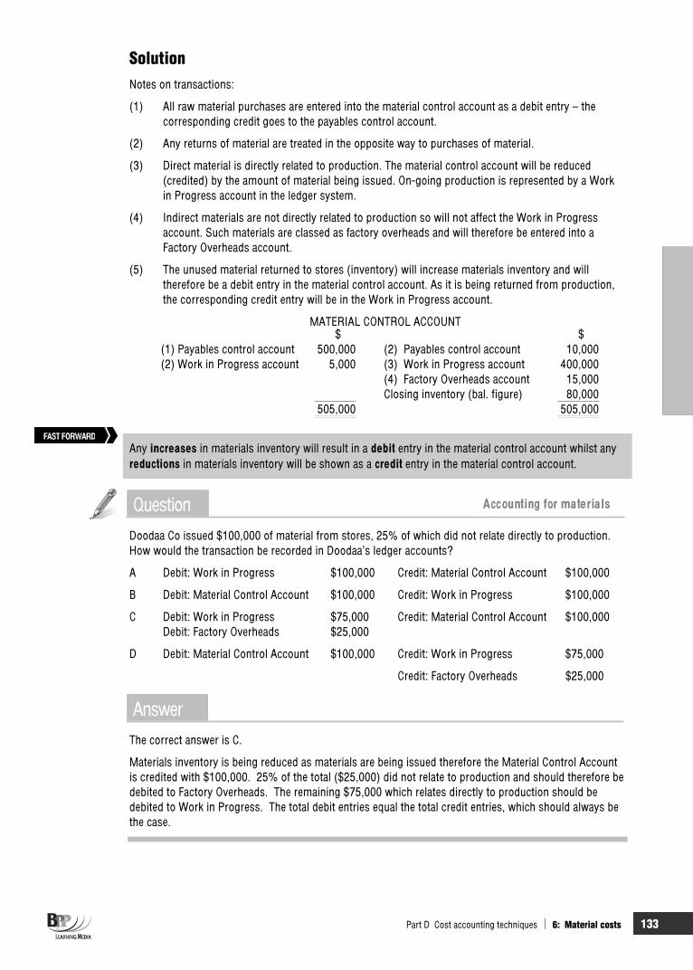
Part D Cost accounting techniques 6: Material costs 133
SolutionNotes on transactions:
(1) All raw material purchases are entered into the material control account as a debit entry – the corresponding credit goes to the payables control account.
(2) Any returns of material are treated in the opposite way to purchases of material.
(3) Direct material is directly related to production. The material control account will be reduced (credited) by the amount of material being issued. On-going production is represented by a Work in Progress account in the ledger system.
(4) Indirect materials are not directly related to production so will not affect the Work in Progress account. Such materials are classed as factory overheads and will therefore be entered into a Factory Overheads account.
(5) The unused material returned to stores (inventory) will increase materials inventory and will therefore be a debit entry in the material control account. As it is being returned from production, the corresponding credit entry will be in the Work in Progress account.
MATERIAL CONTROL ACCOUNT $ $
(1) Payables control account 500,000 (2) Payables control account 10,000(2) Work in Progress account 5,000 (3) Work in Progress account 400,000
(4) Factory Overheads account 15,000Closing inventory (bal. figure) 80,000
505,000 505,000
Any increases in materials inventory will result in a debit entry in the material control account whilst any reductions in materials inventory will be shown as a credit entry in the material control account.
Question Accounting for materials
Doodaa Co issued $100,000 of material from stores, 25% of which did not relate directly to production.How would the transaction be recorded in Doodaa’s ledger accounts?
A Debit: Work in Progress $100,000 Credit: Material Control Account $100,000
B Debit: Material Control Account $100,000 Credit: Work in Progress $100,000
C Debit: Work in Progress $75,000 Credit: Material Control Account $100,000 Debit: Factory Overheads $25,000
D Debit: Material Control Account $100,000 Credit: Work in Progress $75,000
Credit: Factory Overheads $25,000
AnswerThe correct answer is C.
Materials inventory is being reduced as materials are being issued therefore the Material Control Account is credited with $100,000. 25% of the total ($25,000) did not relate to production and should therefore be debited to Factory Overheads. The remaining $75,000 which relates directly to production should be debited to Work in Progress. The total debit entries equal the total credit entries, which should always be the case.
FAST FORWARD
134 6: Material costs Part D Cost accounting techniques
Chapter roundup
Inventory control includes the functions of inventory ordering and purchasing, receiving goods into store, storing and issuing inventory and controlling the level of inventories.
Every movement of material in a business should be documented using the following as appropriate: purchase requisition, purchase order, GRN, materials requisition note, materials transfer note and materials returned note.
The inventory count (stock take) involves counting the physical inventory on hand at a certain date, and then checking this against the balance shown in the inventory records. The inventory count can be carried out on a continuous or periodic basis.
Perpetual inventory refers to a inventory recording system whereby the records (bin cards and stores ledger accounts) are updated for each receipt and issue of inventory as it occurs.
Obsolete inventories are those items which have become out of date and are no longer required. Obsolete items are written off and disposed of.
Inventory costs include purchase costs, holding costs, ordering costs and costs of running out of inventory.
Inventory control levels can be calculated in order to maintain inventories at the optimum level. The three critical control levels are reorder level, minimum level and maximum level.
The economic order quantity (EOQ) is the order quantity which minimises inventory costs. The EOQ can be calculated using a table, graph or formula.
EOQ = H
o
CDC2
The economic batch quantity (EBQ) is a modification of the EOQ and is used when resupply is gradual instead of instantaneous.
EBQ = R)/D_1(C
DC2
H
o
Any increases in materials inventory will result in a debit entry in the material control account whilst any reductions in materials inventory will be shown as a credit entry in the material control account.

Part D Cost accounting techniques 6: Material costs 135
Quick quiz 1 List six objectives of storekeeping.
…………………………………… …………………………………… …………………………………… …………………………………… …………………………………… ……………………………………
2 Free inventory represents………………………………………………………………………….
3 Free inventory is calculated as follows. (Delete as appropriate)
(a) + – Materials in inventory X(b) + – Materials in order X(c) + – Materials requisitioned (not yet issued) X Free inventory balance X
4 How does periodic inventory counting differ from continuous inventory counting?
5 Match up the following.
Reorder quantity Maximum usage maximum lead time
Minimum level Safety inventory + ½ reorder level
Maximum level ? Reorder level – (average usage average lead time)
Average inventory Reorder level + reorder quantity – (minimum usage minimum lead time)
6 EOQ = H
o
CDC2
Where
(a) CH = …………………………………………………..
(b) Co = ..…………………………………………………
(c) D = ………………………………………………….
7 When is the economic batch quantity used?

136 6: Material costs Part D Cost accounting techniques
Answers to quick quiz 1 Speedy issue and receipt of materials
Full identification of all materials at all times Correct location of all materials at all times
Protection of materials from damage and deterioration Provision of secure stores to avoid pilferage, theft and fire
Efficient use of storage space Maintenance of correct inventory levels
Keeping correct and up-to-date records of receipts, issues and inventory levels
2 Inventory that is readily available for future use.
3 (a) + (b) + (c) –
4 Periodic inventory counting. All inventory items physically counted and valued, usually annually.
Continuous inventory counting. Counting and valuing selected items at different times of the year (at least once a year).
5
Reorder quantity Maximum usage maximum lead time
Minimum level Safety inventory + ½ reorder level
Maximum level Reorder level – (average usage average lead time)
Average inventory Reorder level + reorder quantity – (minimum usage minimum lead time)
6 (a) Cost of holding one unit of inventory for one time period (b) Cost of ordering a consignment from a supplier (c) Demand during the time period
7 When resupply of a product is gradual instead of instantaneous.
Now try the questions below from the Exam Question Bank
Number Level Marks Time
Q6 MCQ n/a n/a

137
Labour costs
IntroductionJust as management need to control inventories and operate an appropriate valuation policy in an attempt to control material costs, so too must they be aware of the most suitable remuneration policy for their organisation. We will be looking at a number of methods of remuneration and will consider the various types of incentive scheme that exist. We will also examine the procedures and documents required for the accurate recording of labour costs.Labour turnover will be studied too.
Topic list Syllabus reference
1 Measuring labour activity D2 (a) (f)
2 Remuneration methods D2 (d)
3 Recording labour costs D2 (b)
4 Labour turnover D2 (e)
5 Accounting for labour costs D2 (c) (g)

138 7: Labour costs Part D Cost accounting techniques
Study guide Intellectual level
D2 Accounting for labour
(a) Calculate direct and indirect labour costs 1
(b) Explain the methods used to relate input labour costs to work done 1
(c) Prepare journal and ledger entries to record labour cost inputs and outputs 1
(d) Describe different remuneration methods, time-based systems, piecework systems and individual and group incentive schemes
1
(e) Calculate the level, and analyse the costs and causes of, labour turnover 1
(f) Explain and calculate labour efficiency, capacity and production volume ratios
1
(g) Interpret the entries in the labour account 1
Exam guide You may get a question just on labour costs or on working out an employee's pay or you may have to deal with labour as a component of variable cost or overhead.
1 Measuring labour activity Production and productivity are common methods of measuring labour activity.
1.1 Production and productivity
Production is the quantity or volume of output produced. Productivity is a measure of the efficiency with which output has been produced. An increase in production without an increase in productivity will not reduce unit costs
1.2 Example: Production and productivity Suppose that an employee is expected to produce three units in every hour that he works. The standard rate of productivity is three units per hour, and one unit is valued at 1/3 of a standard hour of output. If, during one week, the employee makes 126 units in 40 hours of work the following comments can be made.
(a) Production in the week is 126 units.
(b) Productivity is a relative measure of the hours actually taken and the hours that should have been taken to make the output.
(i) Either, 126 units should take 42 hours But did take 40 hours Productivity ratio = 42/40 100% = 105%
(ii) Or alternatively, in 40 hours, he should make ( 3) 120 units But did make 126 units Productivity ratio = 126/120 100% = 105%
A productivity ratio greater than 100% indicates that actual efficiency is better than the expected or 'standard' level of efficiency.
FAST FORWARD

Part D Cost accounting techniques 7: Labour costs 139
Standard hour of production is a concept used in standard costing, and means the number of units that can be produced by one worker working in the standard way at the standard rate for one hour.
1.3 Planning and controlling production and productivity Management will wish to plan and control both production levels and labour productivity.
(a) Production levels can be raised as follows.
(i) Working overtime (ii) Hiring extra staff (iii) Sub-contracting some work to an outside firm (iv) Managing the work force so as to achieve more output.
(b) Production levels can be reduced as follows.
(i) Cancelling overtime (ii) Laying off staff
(c) Productivity, if improved, will enable a company to achieve its production targets in fewer hours of work, and therefore at a lower cost.
1.4 Productivity and its effect on cost Improved productivity is an important means of reducing total unit costs. In order to make this point clear, a simple example will be used.
1.4.1 Example: Productivity and its effect on cost
Clooney Co has a production department in its factory consisting of a work team of just two men, Doug and George. Doug and George each work a 40 hour week and refuse to do any overtime. They are each paid $100 per week and production overheads of $400 per week are charged to their work.
(a) In week one, they produce 160 units of output between them. Productivity is measured in units of output per man hour.
Production 160 unitsProductivity (80 man hours) 2 units per man hour Total cost $600 (labour plus overhead) Cost per man hour $7.50Cost per unit $3.75
(b) In week two, management pressure is exerted on Doug and George to increase output and they produce 200 units in normal time.
Production 200 units (up by 25%) Productivity 2.5 units per man hour (up by 25%) Total cost $600Cost per man hour $7.50 (no change) Cost per unit $3.00 (a saving of 20% on the previous cost;
25% on the new cost)
(c) In week three, Doug and George agree to work a total of 20 hours of overtime for an additional $50 wages. Output is again 200 units and overhead charges are increased by $100.
Production 200 units (up 25% on week one) Productivity (100 man hours) 2 units per hour (no change on week one) Total cost ($600 + $50 + $100) $750 Cost per unit $3.75
Key term

140 7: Labour costs Part D Cost accounting techniques
(d) Conclusions
(i) An increase in production without an increase in productivity will not reduce unit costs (week one compared with week three).
(ii) An increase in productivity will reduce unit costs (week one compared with week two).
1.4.2 Automation
Labour cost control is largely concerned with productivity. Rising wage rates have increased automation, which in turn has improved productivity and reduced costs.
Where automation is introduced, productivity is often, but misleadingly, measured in terms of output per man-hour.
1.4.3 Example: Automation
Suppose, for example, that a work-team of six men (240 hours per week) is replaced by one machine (40 hours per week) and a team of four men (160 hours per week), and as a result output is increased from 1,200 units per week to 1,600 units.
Production Man hours Productivity Before the machine 1,200 units 240 5 units per man hour After the machine 1,600 units 160 10 units per man hour
Labour productivity has doubled because of the machine, and employees would probably expect extra pay for this success. For control purposes, however, it is likely that a new measure of productivity is required, output per machine hour, which may then be measured against a standard output for performance reporting.
1.5 Efficiency, capacity and production volume ratios Other measures of labour activity include the following.
Production volume ratio, or activity ratio Efficiency ratio (or productivity ratio) Capacity ratio
Efficiency ratio Capacity ratio = Production volume ratio
taken hours Actualoutput make tohours Expected
budgeted HoursworkedhoursActual
=budgeted Hours
hours standard or expected in measured Output
These ratios are usually expressed as percentages.
1.5.1 Example: Labour activity ratios
Rush and Fluster Co budgets to make 25,000 standard units of output (in four hours each) during a budget period of 100,000 hours.
Actual output during the period was 27,000 units which took 120,000 hours to make.
Required
Calculate the efficiency, capacity and production volume ratios.
Solution
(a) Efficiency ratio 000,120
hours)4000,27( 100% = 90%
(b) Capacity ratio hours000,100 hours000,120
100% = 120%
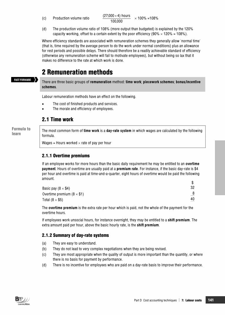
Part D Cost accounting techniques 7: Labour costs 141
(c) Production volume ratio 000,100
hours)4000,27( 100% =108%
(d) The production volume ratio of 108% (more output than budgeted) is explained by the 120% capacity working, offset to a certain extent by the poor efficiency (90% 120% = 108%).
Where efficiency standards are associated with remuneration schemes they generally allow 'normal time' (that is, time required by the average person to do the work under normal conditions) plus an allowance for rest periods and possible delays. There should therefore be a readily achievable standard of efficiency (otherwise any remuneration scheme will fail to motivate employees), but without being so lax that it makes no difference to the rate at which work is done.
2 Remuneration methods There are three basic groups of remuneration method: time work; piecework schemes; bonus/incentiveschemes.
Labour remuneration methods have an effect on the following.
The cost of finished products and services. The morale and efficiency of employees.
2.1 Time work
The most common form of time work is a day-rate system in which wages are calculated by the following formula.
Wages = Hours worked rate of pay per hour
2.1.1 Overtime premiums
If an employee works for more hours than the basic daily requirement he may be entitled to an overtimepayment. Hours of overtime are usually paid at a premium rate. For instance, if the basic day-rate is $4 per hour and overtime is paid at time-and-a-quarter, eight hours of overtime would be paid the following amount.
$Basic pay (8 $4) 32
Overtime premium (8 $1) 8
Total (8 $5) 40
The overtime premium is the extra rate per hour which is paid, not the whole of the payment for the overtime hours.
If employees work unsocial hours, for instance overnight, they may be entitled to a shift premium. The extra amount paid per hour, above the basic hourly rate, is the shift premium.
2.1.2 Summary of day-rate systems
(a) They are easy to understand. (b) They do not lead to very complex negotiations when they are being revised. (c) They are most appropriate when the quality of output is more important than the quantity, or where
there is no basis for payment by performance.(d) There is no incentive for employees who are paid on a day-rate basis to improve their performance.
Formula to learn
FAST FORWARD

142 7: Labour costs Part D Cost accounting techniques
2.2 Piecework schemes
In a piecework scheme, wages are calculated by the following formula. Wages = Units produced Rate of pay per unit
Suppose for example, an employee is paid $1 for each unit produced and works a 40 hour week. Production overhead is added at the rate of $2 per direct labour hour.
Pay Conversion Conversion Weekly production (40 hours) Overhead cost cost per unit
Units $ $ $ $ 40 40 80 120 3.00 50 50 80 130 2.60 60 60 80 140 2.33 70 70 80 150 2.14
As his output increases, his wage increases and at the same time unit costs of output are reduced.
It is normal for pieceworkers to be offered a guaranteed minimum wage, so that they do not suffer loss of earnings when production is low through no fault of their own.
If an employee makes several different types of product, it may not be possible to add up the units for payment purposes. Instead, a standard time allowance is given for each unit to arrive at a total of piecework hours for payment.
Question Weekly pay
Penny Pincher is paid 50c for each towel she weaves, but she is guaranteed a minimum wage of $60 for a 40 hour week. In a series of four weeks, she makes 100, 120, 140 and 160 towels.
Required
Calculate her pay each week, and the conversion cost per towel if production overhead is added at the rate of $2.50 per direct labour hour.
Answer Unit Production Conversion conversion
Week Output Pay overhead cost cost Units $ $ $ $
1 100 (minimum) 60 100 160 1.60 2 120 60 100 160 1.33 3 140 70 100 170 1.21 4 160 80 100 180 1.13
There is no incentive to Penny Pincher to produce more output unless she can exceed 120 units in a week. The guaranteed minimum wage in this case is too high to provide an incentive.
2.2.1 Example: Piecework
An employee is paid $5 per piecework hour produced. In a 35 hour week he produces the following output.
Piecework time allowed per unit
3 units of product A 2.5 hours 5 units of product B 8.0 hours
Formula to learn

Part D Cost accounting techniques 7: Labour costs 143
Required
Calculate the employee's pay for the week.
Solution
Piecework hours produced are as follows.
Product A 3 2.5 hours 7.5 hours Product B 5 8 hours 40.0 hours Total piecework hours 47.5 hours
Therefore employee's pay = 47.5 $5 = $237.50 for the week.
2.2.2 Differential piecework scheme
Differential piecework schemes offer an incentive to employees to increase their output by paying higher rates for increased levels of production. For example:
up to 80 units per week, rate of pay per unit = $1.00 80 to 90 units per week, rate of pay per unit = $1.20 above 90 units per week, rate of pay per unit = $1.30
Employers should obviously be careful to make it clear whether they intend to pay the increased rate on all units produced, or on the extra output only.
2.2.3 Summary of piecework schemes
They enjoy fluctuating popularity. They are occasionally used by employers as a means of increasing pay levels. They are often seen to drive employees to work too hard to earn a satisfactory wage.
Careful inspection of output is necessary to ensure that quality doesn't fall as production increases.
2.3 Bonus/incentive schemes
2.3.1 Introduction
In general, bonus schemes were introduced to compensate workers paid under a time-based system for their inability to increase earnings by working more efficiently. Various types of incentive and bonus schemes have been devised which encourage greater productivity. The characteristics of such schemes are as follows.
(a) Employees are paid more for their efficiency. (b) The profits arising from productivity improvements are shared between employer and employee. (c) Morale of employees is likely to improve since they are seen to receive extra reward for extra effort.
A bonus scheme must satisfy certain conditions to operate successfully.
(a) Its objectives should be clearly stated and attainable by the employees. (b) The rules and conditions of the scheme should be easy to understand.(c) It must win the full acceptance of everyone concerned. (d) It should be seen to be fair to employees and employers..(e) The bonus should ideally be paid soon after the extra effort has been made by the employees. (f) Allowances should be made for external factors outside the employees' control which reduce their
productivity (machine breakdowns, material shortages). (g) Only those employees who make the extra effort should be rewarded. (h) The scheme must be properly communicated to employees.

144 7: Labour costs Part D Cost accounting techniques
We shall be looking at the following types of incentive schemes in detail.
High day rate system Profit sharing schemes Individual bonus schemes Incentive schemes involving shares Group bonus schemes Value added incentive schemes
Some organisations employ a variety of incentive schemes. A scheme for a production labour force may not necessarily be appropriate for white-collar workers. An organisation's incentive schemes may be regularly reviewed, and altered as circumstances dictate.
2.4 High day-rate system
A high day-rate system is a system where employees are paid a high hourly wage rate in the expectation that they will work more efficiently than similar employees on a lower hourly rate in a different company.
2.4.1 Example: High day-rate system
For example if an employee would make 100 units in a 40 hour week if he were paid $2 per hour, but 120 units if he were paid $2.50 per hour, and if production overhead is added to cost at the rate of $2 per direct labour hour, costs per unit of output would be as follows.
(a) Costs per unit of output on the low day-rate scheme would be:
100)4$40(
= $1.60 per unit
(b) Costs per unit of output on the high day-rate scheme would be:
120)50.4$40(
= $1.50 per unit
(c) Note that in this example the labour cost per unit is lower in the first scheme (80c) than in the second (83.3c), but the unit conversion cost (labour plus production overhead) is higher because overhead costs per unit are higher at 80c than with the high day-rate scheme (66.7c).
(d) In this example, the high day-rate scheme would reward both employer (a lower unit cost by 10c) and employee (an extra 50c earned per hour).
2.4.2 Advantages and disadvantages of high day rate schemes
There are two advantages of a high day-rate scheme over other incentive schemes.
(a) It is simple to calculate and easy to understand. (b) It guarantees the employee a consistently high wage.
The disadvantages of such schemes are as follows.
(a) Employees cannot earn more than the fixed hourly rate for their extra effort. In the previous example, if the employee makes 180 units instead of 120 units in a 40 hour week on a high day-rate pay scheme, the cost per unit would fall to $1 but his wage would be the same – 40 hours at $4.50. All the savings would go to benefit the company and none would go to the employee.
(b) There is no guarantee that the scheme will work consistently. The high wages may become the accepted level of pay for normal working, and supervision may be necessary to ensure that a high level of productivity is maintained. Unit costs would rise.
(c) Employees may prefer to work at a normal rate of output, even if this entails accepting the lower wage paid by comparable employers.
Key term

Part D Cost accounting techniques 7: Labour costs 145
2.5 Individual bonus schemes
An individual bonus scheme is a remuneration scheme whereby individual employees qualify for a bonus on top of their basic wage, with each person's bonus being calculated separately.
(a) The bonus is unique to the individual. It is not a share of a group bonus. (b) The individual can earn a bonus by working at an above-target standard of efficiency. (c) The individual earns a bigger bonus the greater his efficiency, although the bonus scheme might
incorporate quality safeguards, to prevent individuals from sacrificing quality standards for the sake of speed and more pay.
To be successful, however, an individual bonus scheme must take account of the following factors.
(a) Each individual should be rewarded for the work done by that individual. This means that each person's output and time must be measured separately. Each person must therefore work without the assistance of anyone else.
(b) Work should be fairly routine, so that standard times can be set for jobs. (c) The bonus should be paid soon after the work is done, to provide the individual with the incentive
to try harder.
2.6 Group bonus schemes
A group bonus scheme is an incentive plan which is related to the output performance of an entire group of workers, a department, or even the whole factory.
Where individual effort cannot be measured, and employees work as a team, an individual incentive scheme is impracticable but a group bonus scheme would be feasible.
The other advantages of group bonus schemes are as follows.
(a) They are easier to administer because they reduce the clerical effort required to measure output and calculate individual bonuses.
(b) They increase co-operation between fellow workers. (c) They have been found to reduce accidents, spoilage, waste and absenteeism.
Serious disadvantages would occur in the following circumstances.
(a) The employee groups demand low efficiency standards as a condition of accepting the scheme. (b) Individual employees are browbeaten by their fellow workers for working too slowly.
2.7 Profit-sharing schemes
A profit sharing scheme is a scheme in which employees receive a certain proportion of their company's year-end profits (the size of their bonus being related to their position in the company and the length of their employment to date).
The advantage of these schemes is that the company will only pay what it can afford out of actual profits and the bonus can be paid also to non-production personnel.
The disadvantages of profit sharing are as follows.
(a) Employees must wait until the year end for a bonus. The company is therefore expecting a long-term commitment to greater efforts and productivity from its workers without the incentive of immediate reward.
(b) Factors affecting profit may be outside the control of employees, in spite of their greater efforts. (c) Too many employees are involved in a single scheme for the scheme to have a great motivating
effect on individuals.
Key term
Key term
Key term

146 7: Labour costs Part D Cost accounting techniques
2.7.1 Incentive schemes involving shares
It is becoming increasingly common for companies to use their shares, or the right to acquire them, as a form of incentive.
A share option scheme is a scheme which gives its members the right to buy shares in the company for which they work at a set date in the future and at a price usually determined when the scheme is set up.
An employee share ownership plan is a scheme which acquires shares on behalf of a number of employees, and it must distribute these shares within a certain number of years of acquisition.
Some governments have encouraged companies to set up schemes of this nature in the hope that workers will feel they have a stake in the company which employs them. The disadvantages of these schemes are as follows.
(a) The benefits are not certain, as the market value of shares at a future date cannot realistically be predicted in advance.
(b) The benefits are not immediate, as a scheme must be in existence for a number of years before members can exercise their rights.
2.7.2 Value added incentive schemes
Value added is an alternative to profit as a business performance measure and it can be used as the basis of an incentive scheme. It is calculated as follows.
Value added = sales – cost of bought-in materials and services
The advantage of value added over profit as the basis for an incentive scheme is that it excludes any bought-in costs, and is affected only by costs incurred internally, such as labour.
A basic value added figure would be agreed as the target for a business, and some of any excess value added earned would be paid out as a bonus. For example, it could be agreed that value added should be, say, treble the payroll costs and a proportion of any excess earned, say one third, would be paid as bonus.
Payroll costs for month $40,000 Therefore, value added target ( 3) $120,000Value added achieved $150,000Therefore, excess value added $30,000Employee share to be paid as bonus $10,000
2.7.3 Example: incentive schemes
Swetton Tyres Co manufactures a single product. Its work force consists of 10 employees, who work a 36-hour week exclusive of lunch and tea breaks. The standard time required to make one unit of the product is two hours, but the current efficiency (or productivity) ratio being achieved is 80%. No overtime is worked, and the work force is paid $4 per attendance hour.
Because of agreements with the work force about work procedures, there is some unavoidable idle time due to bottlenecks in production, and about four hours per week per person are lost in this way.
The company can sell all the output it manufactures, and makes a 'cash profit' of $20 per unit sold, deducting currently achievable costs of production but before deducting labour costs.
An incentive scheme is proposed whereby the work force would be paid $5 per hour in exchange for agreeing to new work procedures that would reduce idle time per employee per week to two hours and also raise the efficiency ratio to 90%.
Required
Evaluate the incentive scheme from the point of view of profitability.
Key terms
Key term

Part D Cost accounting techniques 7: Labour costs 147
Solution
The current situation
Hours in attendance 10 36 = 360 hours Hours spent working 10 32 = 320 hours
Units produced, at 80% efficiency 2
32010080
= 128 units
$Cash profits before deducting labour costs (128 $20) 2,560
Less labour costs ($4 360 hours) 1,440Net profit 1,120
The incentive scheme
Hours spent working 10 34 = 340 hours
Units produced, at 90% efficiency 2
34010090
= 153 units
$Cash profits before deducting labour costs (153 $20) 3,060
Less labour costs ($5 360) 1,800Net profit 1,260
In spite of a 25% increase in labour costs, profits would rise by $140 per week. The company and the workforce would both benefit provided, of course, that management can hold the work force to their promise of work reorganisation and improved productivity.
Question Labour cost
The following data relate to work at a certain factory.
Normal working day 8 hours Basic rate of pay per hour $6 Standard time allowed to produce 1 unit 2 minutes Premium bonus 75% of time saved at basic rate
What will be the labour cost in a day when 340 units are made?
A $48 B $51 C $63 D $68
AnswerStandard time for 340 units ( 2 minutes) 680 minutesActual time (8 hours per day) 480 minutesTime saved 200 minutes
$Bonus = 75% 200 minutes $6 per hour 15Basic pay = 8 hours $6 48Total labour cost 63
Therefore the correct answer is C.
Using basic MCQ technique you can eliminate option A because this is simply the basic pay without consideration of any bonus. You can also eliminate option D, which is based on the standard time allowance without considering the basic pay for the eight-hour day. Hopefully your were not forced to guess, but had you been you would have had a 50% chance of selecting the correct answer (B or C) instead of a 25% chance because you were able to eliminate two of the options straightaway.
148 7: Labour costs Part D Cost accounting techniques
3 Recording labour costs Labour attendance time is recorded on, for example, an attendance record or clock card. Job time may be recorded on daily time sheets, weekly time sheets or job cards depending on the circumstances. The manual recording of times on time sheets or job cards is, however, liable to error or even deliberate deception and may be unreliable. The labour cost of pieceworkers is recorded on a piecework ticket/operation card.
3.1 Organisation for controlling and measuring labour costs Several departments and management groups are involved in the collection, recording and costing of labour. These include the following.
Personnel Wages Production planning Cost accounting Timekeeping
3.2 Personnel department The personnel department is responsible for the following:
Engagement, transfer and discharge of employees. Classification and method of remuneration.
The department is headed by a professional personnel officer trained in personnel management, labour laws, company personnel policy and industry conditions who should have an understanding of the needs and problems of the employees.
When a person is engaged a personnel record card should be prepared showing full personal particulars, previous employment, medical category and wage rate. Other details to be included are social security number, address, telephone number, transfers, promotions, changes in wage rates, sickness and accidents and, when an employee leaves, the reason for leaving.
Personnel departments sometimes maintain records of overtime and shift working. Overtime has to be sanctioned by the works manager or personnel office who advise the time-keepers who control the time booked.
The personnel department is responsible for issuing reports to management on normal and overtime hours worked, absenteeism and sickness, lateness, labour turnover and disciplinary action.
3.3 Production planning department This department is responsible for the following.
Scheduling work Issuing job orders to production departments Chasing up jobs when they run late
3.4 Timekeeping department The timekeeping department is responsible for recording the attendance time and job time of the following.
The time spent in the factory by each worker The time spent by each worker on each job
Such timekeeping provides basic data for statutory records, payroll preparation, labour costs of an operation or overhead distribution (where based on wages or labour hours) and statistical analysis of labour records for determining productivity and control of labour costs.
FAST FORWARD

Part D Cost accounting techniques 7: Labour costs 149
3.5 Attendance time The bare minimum record of employees' time is a simple attendance record showing days absent because of holiday, sickness or other reason. A typical record of attendance is shown as follows.
It is also necessary to have a record of the following.
Time of arrival Time of departure Time of breaks
These may be recorded as follows.
In a signing-in book By using a time recording clock which stamps the time on a clock card By using swipe cards (which make a computer record)
An example of a clock card is shown as follows.

150 7: Labour costs Part D Cost accounting techniques
3.6 Job time Continuous production. Where routine, repetitive work is carried out it might not be practical to record the precise details. For example if a worker stands at a conveyor belt for seven hours his work can be measured by keeping a note of the number of units that pass through his part of the process during that time.
Job costing. When the work is not of a repetitive nature the records required might be one or several of the following.
(a) Daily time sheets. A time sheet is filled in by the employee as a record of how their time has been spent. The total time on the time sheet should correspond with time shown on the attendance record.
(b) Weekly time sheets. These are similar to daily time sheets but are passed to the cost office at the end of the week. An example of a weekly timesheet is shown below.
(c) Job cards. Cards are prepared for each job or batch. When an employee works on a job he or she records on the job card the time spent on that job. Job cards are therefore likely to contain entries relating to numerous employees. On completion of the job it will contain a full record of the times and quantities involved in the job or batch. A typical job card is shown as follows.
A job card will be given to the employee, showing the work to be done and the expected time it should take. The employee will record the time started and time finished for each job. Breaks for tea and lunch may be noted on the card, as standard times, by the production planning department. The hours actually taken and the cost of those hours will be calculated by the accounting department.

Part D Cost accounting techniques 7: Labour costs 151
Piecework. The wages of pieceworkers and the labour cost of work done by them is determined from what is known as a piecework ticket or an operation card. The card records the total number of items (or 'pieces') produced and the number of rejects. Payment is only made for 'good' production.
Note that the attendance record of a pieceworker is required for calculations of holidays, sick pay and so on.
Other types of work. Casual workers are paid from job cards or time sheets. Time sheets are also used where outworkers are concerned.
Office work can be measured in a similar way, provided that the work can be divided into distinct jobs. Firms of accountants and advertising agencies, for example, book their staff time to individual clients and so make use of time sheets for salaried staff.
3.7 Salaried labour Even though salaried staff are paid a flat rate monthly, they may be required to prepare timesheets. The reasons are as follows.
(a) Timesheets provide management with information (eg product costs). (b) Timesheet information may provide a basis for billing for services provided (eg service firms where
clients are billed based on the number of hours work done). (c) Timesheets are used to record hours spent and so support claims for overtime payments by
salaried staff.
An example of a timesheet (as used in the service sector) is shown as follows.

152 7: Labour costs Part D Cost accounting techniques
3.8 Idle time
Idle time has a cost because employees will still be paid their basic wage or salary for these unproductive hours and so there should be a record of idle time.
Idle time occurs when employees cannot get on with their work, through no fault of their own. Examples are as follows.
Machine breakdowns Shortage of work
A record of idle time may simply comprise an entry on time sheets coded to 'idle time' generally, or separate idle time cards may be prepared. A supervisor might enter the time of a stoppage, its cause, its duration and the employees made idle on an idle time record card. Each stoppage should have a reference number which can be entered on time sheets or job cards.
3.9 Wages department Responsibilities of the payroll department include the following.
Preparation of the payroll and payment of wages. Maintenance of employee records. Summarising wages cost for each cost centre. Summarising the hours worked for each cost centre. Summarising other payroll information eg bonus payment, pensions etc. Providing an internal check for the preparation and payout of wages.
Attendance cards are the basis for payroll preparation. For time workers, the gross wage is the product of time attended and rate of pay. To this is added any overtime premium or bonus. For piece workers, gross wages are normally obtained by the product of the number of good units produced and the unit rate, with any premiums, bonuses and allowances for incomplete jobs added.
After calculation of net pay, a pay slip is prepared showing all details of earnings and deductions. The wage envelope or the attendance card may be used for this purpose.
When the payroll is complete, a coin and note analysis is made and a cheque drawn to cover the total amount. On receipt of the cash, the pay envelopes are made up and sealed. A receipt is usually obtained on payout (the attendance card can be used). Wages of absentees are retained until claimed by an authorised person.
FAST FORWARD

Part D Cost accounting techniques 7: Labour costs 153
Internal checks are necessary to prevent fraud. One method is to distribute the payroll work so that no person deals completely with any transaction. All calculations should be checked on an adding machine where possible. Makeup of envelopes should not be done by persons who prepare the payroll. The cashier should reconcile his analysis with the payroll summary.
3.10 Cost accounting department The cost accounting department has the following responsibilities.
The accumulation and classification of all cost data (which includes labour costs). Preparation of cost data reports for management. Analysing labour information on time cards and payroll.
In order to establish the labour cost involved in products, operations, jobs and cost centres, the following documents are used.
Clock cards Idle time cards Job cards Payroll
Analyses of labour costs are used for the following.
(a) Charging wages directly attributable to production to the appropriate job or operation.
(b) Charging wages which are not directly attributable to production as follows.
(i) Idle time of production workers is charged to indirect costs as part of the overheads. (ii) Wages costs of supervisors, or store assistants are charged to the overhead costs of the
relevant department.
(c) Producing idle time reports which show a summary of the hours lost through idle time, and the cause of the idle time. Idle time may be analysed as follows.
(i) Controllable eg lack of materials. (ii) Uncontrollable eg power failure.
3.11 Idle time ratio
Idle time ratio = hours Total
hours Idle 100%
The idle time ratio is useful because it shows the proportion of available hours which were lost as a result of idle time.
Make sure you understand the distinction between direct and indirect labour costs and the classification of overtime premium.
4 Labour turnover
Labour turnover is the rate at which employees leave a company and this rate should be kept as low as possible. The cost of labour turnover can be divided into preventative and replacement costs.
4.1 The reasons for labour turnover Some employees will leave their job and go to work for another company or organisation. Sometimes the reasons are unavoidable.
Illness or accidents A family move away from the locality Marriage, pregnancy or difficulties with child care provision Retirement or death
Formula to learn
FAST FORWARD
Exam focus point
154 7: Labour costs Part D Cost accounting techniques
Other causes of labour turnover are to some extent controllable.
Paying a lower wage rate than is available elsewhere. Requiring employees to work in unsafe or highly stressful conditions. Requiring employees to work uncongenial hours. Poor relationships between management and staff. Lack of opportunity for career enhancement. Requiring employees to work in inaccessible places (eg no public transport). Discharging employees for misconduct, bad timekeeping or unsuitability.
4.2 Measuring labour turnover
Labour turnover is a measure of the number of employees leaving/being recruited in a period of time expressed as a percentage of the total labour force.
Labour turnover rate = period in employees of number Average
tsReplacemen 100%
4.3 Example : Labour turnover rate Revolving Doors Inc had a staff of 2,000 at the beginning of 20X1 and, owing to a series of redundancies caused by the recession, 1,000 at the end of the year. Voluntary redundancy was taken by 1,500 staff at the end of June, 500 more than the company had anticipated, and these excess redundancies were immediately replaced by new joiners.
The labour turnover rate is calculated as follows.
Rate = 2)000,1000,2(
500 100% = 33%
4.4 The costs of labour turnover The costs of labour turnover can be large and management should attempt to keep labour turnover as low as possible so as to minimise these costs. The cost of labour turnover may be divided into the following.
Preventative costs Replacement costs
4.4.1 Replacement costs
These are the costs incurred as a result of hiring new employees. and they include the following.
Cost of selection and placement Inefficiency of new labour; productivity will be lower Costs of training Loss of output due to delay in new labour becoming available Increased wastage and spoilage due to lack of expertise among new staff The possibility of more frequent accidents at work Cost of tool and machine breakages
4.4.2 Preventative costs
These are costs incurred in order to prevent employees leaving and they include the following.
Cost of personnel administration incurred in maintaining good relationships Cost of medical services including check-ups, nursing staff and so on Cost of welfare services, including sports facilities and canteen meals Pension schemes providing security to employees
Key term
Formula to learn

Part D Cost accounting techniques 7: Labour costs 155
4.5 The prevention of high labour turnover Labour turnover will be reduced by the following actions.
Paying satisfactory wages Offering satisfactory hours and conditions of work Creating a good informal relationship between members of the workforce Offering good training schemes and a well-understood career or promotion ladder Improving the content of jobs to create job satisfaction Proper planning so as to avoid redundancies Investigating the cause of an apparently high labour turnover
5 Accounting for labour costs We will use an example to briefly review the principal bookkeeping entries for wages.
5.1 Example: The wages control account The following details were extracted from a weekly payroll for 750 employees at a factory.
Analysis of gross pay Direct Indirect workers workers Total
$ $ $ Ordinary time 36,000 22,000 58,000 Overtime: basic wage 8,700 5,430 14,130 premium 4,350 2,715 7,065 Shift allowance 3,465 1,830 5,295 Sick pay 950 500 1,450 Idle time 3,200 – 3,200
56,665 32,475 89,140 Net wages paid to employees $45,605 $24,220 $69,825
Required
Prepare the wages control account for the week.
Solution(a) The wages control account acts as a sort of 'collecting place' for net wages paid and deductions
made from gross pay. The gross pay is then analysed between direct and indirect wages.
(b) The first step is to determine which wage costs are direct and which are indirect. The direct wages will be debited to the work in progress account and the indirect wages will be debited to the production overhead account.
(c) There are in fact only two items of direct wages cost in this example, the ordinary time ($36,000) and the basic overtime wage ($8,700) paid to direct workers. All other payments (including the overtime premium) are indirect wages.
(d) The net wages paid are debited to the control account, and the balance then represents the deductions which have been made for tax, social insurance, and so on.

156 7: Labour costs Part D Cost accounting techniques
WAGES CONTROL ACCOUNT $ $ Bank: net wages paid 69,825 Work in progress – direct labour 44,700 Deductions control accounts* Production overhead control: ($89,140 $69,825) 19,315 Indirect labour 27,430
Overtime premium 7,065 Shift allowance 5,295 Sick pay 1,450
Idle time 3,20089,140 89,140
* In practice there would be a separate deductions control account for each type of deduction made (for example, tax and social insurance).
5.2 Direct and indirect labour costs We had a brief look at direct and indirect labour costs in Chapter 3. Have a go at the following questions to remind yourself about the classification of labour costs.
Question Direct and indirect costs
A direct labour employee's wage in week 5 consists of the following. $
(a) Basic pay for normal hours worked, 36 hours at $4 per hour = 144
(b) Pay at the basic rate for overtime, 6 hours at $4 per hour = 24
(c) Overtime shift premium, with overtime paid at time-and-a-quarter ¼ 6 hours $4 per hour = 6
(d) A bonus payment under a group bonus (or 'incentive') scheme – bonus for the month = 30
Total gross wages in week 5 for 42 hours of work 204
Required
Establish which costs are direct costs and which are indirect costs.
AnswerItems (a) and (b) are direct labour costs of the items produced in the 42 hours worked in week 5.
Overtime premium, item (c), is usually regarded as an overhead expense, because it is 'unfair' to charge the items produced in overtime hours with the premium. Why should an item made in overtime be more costly just because, by chance, it was made after the employee normally clocks off for the day?
Group bonus scheme payments, item (d), are usually overhead costs, because they cannot normally be traced directly to individual products or jobs.
In this example, the direct labour employee costs were $168 in direct costs and $36 in indirect costs.
Question Overtime
Jaffa Co employs two types of labour: skilled workers, considered to be direct workers, and semi-skilled workers considered to be indirect workers. Skilled workers are paid $10 per hour and semi-skilled $5 per hour.
The skilled workers have worked 20 hours overtime this week, 12 hours on specific orders and 8 hours on general overtime. Overtime is paid at a rate of time and a quarter.

Part D Cost accounting techniques 7: Labour costs 157
The semi-skilled workers have worked 30 hours overtime, 20 hours for a specific order at a customer's request and the rest for general purposes. Overtime again is paid at time and a quarter.
What would be the total overtime pay considered to be a direct cost for this week?
A $275 C $375 B $355 D $437.50
AnswerDirect cost Indirect cost
$ $Skilled workers Specific overtime (12 hours $10 1.25) 150General overtime (8 hours $10 1) 80
(8 hours $10 0.25) 20 Semi-skilled workers Specific overtime (20 hours $5 1.25) 125General overtime (10 hours $5 1.25) 62.50
355 82.50
The correct answer is therefore B.
If you selected option A, you forgot to include the direct cost of the general overtime of $80 for the skilled workers.
If you selected option C, you included the overtime premium for skilled workers' general overtime of $20.
If you selected option D, you calculated the total of direct cost + indirect cost instead of the direct cost.
The study guide for this paper states that candidates should be able to explain the difference between and calculate direct and indirect labour costs.
Chapter roundup
Production is the quantity or volume of output produced. Productivity is a measure of the efficiency with which output has been produced. An increase in production without an increase in productivity will not reduce unit costs.
There are three basic groups of remuneration method: time work; piecework schemes; and bonus/incentive schemes.
Labour attendance time is recorded on, for example, an attendance record or clock card. Job time may be recorded on daily time sheets, weekly time sheets or job cards depending on the circumstances. The manual recording of times on time sheets or job cards, is however, liable to error or even deliberate deception and may be unreliable. The labour cost of pieceworkers is recorded on a piecework ticket/operation card.
Idle time has a cost because employees will still be paid their basic wage or salary for these unproductive hours and so there should be a record of idle time.
Labour turnover is the rate at which employees leave a company and this rate should be kept as low as possible. The cost of labour turnover can be divided into preventative and replacement costs.
Exam focus point

158 7: Labour costs Part D Cost accounting techniques
Quick quiz 1 Distinguish between the terms production and productivity. 2 List five types of incentive scheme. 3 What are the requirements for a successful individual bonus scheme? 4 What is a value added incentive scheme? 5 When does idle time occur? 6 What are the responsibilities of a typical wages department? 7 Define the idle time ratio. 8 List six methods of reducing labour turnover.
Answers to quick quiz 1 Production is the quantity or volume of output produced
Productivity is a measure of the efficiency with which output has been produced
2 Any five from: High day rate system Profit sharing schemes Individual bonus schemes Incentive schemes involving shares Group bonus schemes Value added incentive schemes
3 Each individual should be rewarded for the work done by that individual Work should be fairly routine, so that standard times can be set for jobs The bonus should be paid soon after the work is done
4 Value added is an alternative to profit as a business performance measure and it can be used as the basis of an incentive scheme
Value added = Sales – cost of bought-in materials and services
5 Idle time occurs when employees cannot get on with their work, through no fault of their own, for example when machines break down or there is a shortage of work.
6 Preparation of the payroll and payment of wages Maintenance of employee records Summarising wages cost for each cost centre Summarising the hours worked for each cost centre Summarising other payroll information, eg bonus payment, pensions etc Providing an internal check for the preparation and payout of wages
7 Idle time ratio = hours Total
hours Idle 100%
8 Any six from:
Paying satisfactory wages Offering satisfactory hours and conditions of work Creating a good informal relationship between members of the workforce Offering good training schemes and a well-understood career or promotion ladder Improving the content of jobs to create job satisfaction Proper planning so as to avoid redundancies Investigating the cause of an apparently high labour turnover
Now try the questions below from the Exam Question Bank
Number Level Marks Time
Q7 MCQ n/a n/a
159
Overheads and absorption costing
IntroductionAbsorption costing is a method of accounting for overheads. It is basically a method of sharing out overheads incurred amongst units produced.
This chapter begins by explaining why absorption costing might be necessary and then provides an overview of how the cost of a unit of product is built up under a system of absorption costing. A detailed analysis of this costing method is then provided, covering the three stages of absorption costing: allocation, apportionment and absorption.
Topic list Syllabus reference
1 Overheads D3 (a)
2 Absorption costing: an introduction D3 (b)
3 Overhead allocation D3 (c)
4 Overhead apportionment D3 (d)
5 Overhead absorption D3 (e)
6 Blanket absorption rates and departmental absorption rates D3 (e)
7 Over and under absorption of overheads D3 (g)
8 Ledger entries relating to overheads D3 (f)
9 Non-manufacturing overheads D3 (h)

160 8: Overheads and absorption costing Part D Cost accounting techniques
Study guide Intellectual level
D3 Accounting for overheads 1
(a) Explain the different treatment of direct and indirect expenses 1
(b) Describe the procedures involved in determining production overhead absorption rates
1
(c) Allocate and apportion production overheads to cost centres using an appropriate basis
1
(d) Reapportion service centre costs including the use of the reciprocal method 2
(e) Select, apply and discuss appropriate bases for absorption rates 2
(f) Prepare journal and ledger entries for manufacturing overheads incurred and absorbed
1
(g) Calculate and explain under– and over-absorbed overheads 1
(h) Apply methods of relating non-production overheads to cost units 1
Exam guide Overhead apportionment and absorption is one of the most important topics in your Management Accounting studies and is almost certain to appear in the exam. Make sure that you study the contents of this chapter and work through the calculations very carefully.
1 Overheads
Overhead is the cost incurred in the course of making a product, providing a service or running a department, but which cannot be traced directly and in full to the product, service or department.
Overhead is actually the total of the following.
Indirect materials Indirect expenses Indirect labour
The total of these indirect costs is usually split into the following categories.
Production Selling and distribution Administration
In cost accounting there are two schools of thought as to the correct method of dealing with overheads.
Absorption costing Marginal costing
2 Absorption costing: an introduction
The objective of absorption costing is to include in the total cost of a product an appropriate share of the organisation's total overhead. An appropriate share is generally taken to mean an amount which reflects the amount of time and effort that has gone into producing a unit or completing a job.
An organisation with one production department that produces identical units will divide the total overheads among the total units produced. Absorption costing is a method for sharing overheads between different products on a fair basis.
FAST FORWARD
FAST FORWARD

Part D Cost accounting techniques 8: Overheads and absorption costing 161
2.1 Is absorption costing necessary? Suppose that a company makes and sells 100 units of a product each week. The prime cost per unit is $6 and the unit sales price is $10. Production overhead costs $200 per week and administration, selling and distribution overhead costs $150 per week. The weekly profit could be calculated as follows.
$ $Sales (100 units $10) 1,000Prime costs (100 $6) 600Production overheads 200Administration, selling and distribution costs 150
950Profit 50
In absorption costing, overhead costs will be added to each unit of product manufactured and sold. $ per unit
Prime cost per unit 6Production overhead ($200 per week for 100 units) 2Full factory cost 8
The weekly profit would be calculated as follows. $
Sales 1,000Less factory cost of sales 800Gross profit 200Less administration, selling and distribution costs 150Net profit 50
Sometimes, but not always, the overhead costs of administration, selling and distribution are also added to unit costs, to obtain a full cost of sales.
$ per unitPrime cost per unit 6.00Factory overhead cost per unit 2.00Administration etc costs per unit 1.50Full cost of sales 9.50
The weekly profit would be calculated as follows. $
Sales 1,000Less full cost of sales 950Profit 50
It may already be apparent that the weekly profit is $50 no matter how the figures have been presented. So, how does absorption costing serve any useful purpose in accounting?
The theoretical justification for using absorption costing is that all production overheads are incurred in the production of the organisation's output and so each unit of the product receives some benefit from these costs. Each unit of output should therefore be charged with some of the overhead costs.
2.2 Practical reasons for using absorption costing
The main reasons for using absorption costing are for inventory valuations, pricing decisions, and establishing the profitability of different products.
(a) Inventory valuations. Inventory in hand must be valued for two reasons.
(i) For the closing inventory figure in the statement of financial position
(ii) For the cost of sales figure in the statement of comprehensive income
The valuation of inventory will affect profitability during a period because of the way in which the cost of sales is calculated.
FAST FORWARD

162 8: Overheads and absorption costing Part D Cost accounting techniques
The cost of goods produced + the value of opening inventories – the value of closing inventories = the cost of goods sold.
In our example, closing inventories might be valued at prime cost ($6), but in absorption costing, they would be valued at a fully absorbed factory cost, $8 per unit. (They would not be valued at $9.50, the full cost of sales, because the only costs incurred in producing goods for finished inventory are factory costs.)
(b) Pricing decisions. Many companies attempt to fix selling prices by calculating the full cost of production or sales of each product, and then adding a margin for profit. In our example, the company might have fixed a gross profit margin at 25% on factory cost, or 20% of the sales price, in order to establish the unit sales price of $10. 'Full cost plus pricing' can be particularly useful for companies which do jobbing or contract work, where each job or contract is different, so that a standard unit sales price cannot be fixed. Without using absorption costing, a full cost is difficult to ascertain.
(c) Establishing the profitability of different products. This argument in favour of absorption costing is more contentious, but is worthy of mention here. If a company sells more than one product, it will be difficult to judge how profitable each individual product is, unless overhead costs are shared on a fair basis and charged to the cost of sales of each product.
2.3 International Accounting Standard 2 (IAS 2)Absorption costing is recommended in financial accounting by IAS 2 Inventories. IAS 2 deals with financial accounting systems. The cost accountant is (in theory) free to value inventories by whatever method seems best, but where companies integrate their financial accounting and cost accounting systems into a single system of accounting records, the valuation of closing inventories will be determined by IAS 2.
IAS 2 states that costs of all inventories should comprise those costs which have been incurred in the normal course of business in bringing the inventories to their 'present location and condition'. These costs incurred will include all related production overheads, even though these overheads may accrue on a time basis. In other words, in financial accounting, closing inventories should be valued at full factory cost, and it may therefore be convenient and appropriate to value inventories by the same method in the cost accounting system.
2.4 Absorption costing stages
The three stages of absorption costing are:
Allocation Absorption Apportionment
We shall now begin our study of absorption costing by looking at the process of overhead allocation.
3 Overhead allocation 3.1 Introduction
Allocation is the process by which whole cost items are charged direct to a cost unit or cost centre.
Cost centres may be one of the following types.
(a) A production department, to which production overheads are charged (b) A production area service department, to which production overheads are charged (c) An administrative department, to which administration overheads are charged
FAST FORWARD
FAST FORWARD

Part D Cost accounting techniques 8: Overheads and absorption costing 163
(d) A selling or a distribution department, to which sales and distribution overheads are charged (e) An overhead cost centre, to which items of expense which are shared by a number of
departments, such as rent and rates, heat and light and the canteen, are charged
The following costs would therefore be charged to the following cost centres via the process of allocation.
Direct labour will be charged to a production cost centre. The cost of a warehouse security guard will be charged to the warehouse cost centre. Paper (recording computer output) will be charged to the computer department. Costs such as the canteen are charged direct to various overhead cost centres.
3.2 Example: Overhead allocationConsider the following costs of a company.
Wages of the foreman of department A $200Wages of the foreman of department B $150Indirect materials consumed in department A $50Rent of the premises shared by departments A and B $300
The cost accounting system might include three overhead cost centres.
Cost centre: 101 Department A 102 Department B 201 Rent
Overhead costs would be allocated directly to each cost centre, ie $200 + $50 to cost centre 101, $150 to cost centre 102 and $300 to cost centre 201. The rent of the factory will be subsequently shared between the two production departments, but for the purpose of day to day cost recording, the rent will first of all be charged in full to a separate cost centre.
4 Overhead apportionment
Apportionment is a procedure whereby indirect costs are spread fairly between cost centres. Service cost centre costs may be apportioned to production cost centres by using the reciprocal method.
The following question will be used to illustrate the overhead apportionment process.
4.1 Example: Overhead apportionment - Swotathon Swotathon Inc has two production departments (A and B) and two service departments (maintenance and stores). Details of next year’s budgeted overheads are shown below.
Total ($) Heat and light 19,200Repair costs 9,600 Machinery Depreciation 54,000Rent and rates 38,400Canteen 9,000 Machinery insurance 25,000
Details of each department are as follows.
A B Maintenance Stores Total Floor area (m2) 6,000 4,000 3,000 2,000 15,000 Machinery book value ($000) 48 20 8 4 80 Number of employees 50 40 20 10 120 Allocated overheads ($000) 15 20 12 5 50
Service departments’ services were used as follows.
FAST FORWARD

164 8: Overheads and absorption costing Part D Cost accounting techniques
A B Maintenance Stores TotalMaintenance hours worked 5,000 4,000 ---- 1,000 10,000 Number of stores requisitions 3,000 1,000 ---- ---- 4,000
4.2 Stage 1: Apportioning general overheads Overhead apportionment follows on from overhead allocation. The first stage of overhead apportionment is to identify all overhead costs as production department, production service department, administration or selling and distribution overhead. The costs for heat and light, rent and rates, the canteen and so on (ie costs allocated to general overhead cost centres) must therefore be shared out between the other cost centres.
4.2.1 Bases of apportionment It is considered important that overhead costs should be shared out on a fair basis. You will appreciate that because of the complexity of items of cost it is rarely possible to use only one method of apportioning costs to the various departments of an organisation. The bases of apportionment for the most usual cases are given below.
Overhead to which the basis applies Basis
Rent, rates, heating and light, repairs and depreciation of buildings
Floor area occupied by each cost centre
Depreciation, insurance of equipment Cost or book value of equipment
Personnel office, canteen, welfare, wages and cost offices, first aid
Number of employees, or labour hours worked in each cost centre
Note that heating and lighting may also be apportioned using volume of space occupied by each cost centre.
4.2.2 Example: Swotathon
Using the Swotathon question above, show how overheads should be apportioned between the four departments.
Solution
Item of cost Basis of Departmentapportionment Mainten-
A B ance Stores$ $ $ $
Heat and light Floor area 7,680 5,120 3,840 2,560Repair costs Floor area 3,840 2,560 1,920 1,280Machine depn Machinery value 32,400 13,500 5,400 2,700Rent and rates Floor area 15,360 10,240 7,680 5,120Canteen No of employees 3,750 3,000 1,500 750Machine insurance Machinery value 15,000 6,250 2,500 1,250Total 78,030 40,670 22,840 13,660
Workings
Overhead apportioned by floor area
Overhead apportioned to department = areafloorTotal
departmentbyoccupiedareaFloor total overhead
For example:
Heat and light apportioned to Dept A = 000,15000,6
19,200 = $7,680
Part D Cost accounting techniques 8: Overheads and absorption costing 165
Overheads apportioned by machinery value
Overheads apportioned to department = machinery of valueTotal
machinerys'departmentofValue total overhead
Overheads apportioned by number of employees
Overheads apportioned to department = employees of no Total
departmentinemployeesofNo total overhead
4.3 Stage 2 – Apportion service department costs Only production departments produce goods that will ultimately be sold. In order to calculate a correct price for these goods, we must determine the total cost of producing each unit – that is, not just the cost of the labour and materials that are directly used in production, but also the indirect costs of services provided by such departments as maintenance, stores and canteen.
Our aim is to apportion all the service department costs to the production departments, in one of three ways.
(a) The direct method, where the service centre costs are apportioned to production departments only. (b) The step-down method, where each service centre’s costs are not only apportioned to production
departments but to some (but not all) of the other service centres that make use of the services provided.
(c) The repeated distribution (or reciprocal) method, where service centre costs are apportioned to both the production departments and service departments that use the services. The service centre costs are then gradually apportioned to the production departments. This method is used only when service departments work for each other – that is, service departments use each other’s services (for example, the maintenance department will use the canteen, whilst the canteen may rely on the maintenance department to ensure its equipment is functioning properly or to replace bulbs, plugs, etc).
The direct and step-down methods are not examinable.
Remember that all service department costs must be allocated – that is, both general overheads that were apportioned and those overheads that are specific to the individual departments.
4.3.1 Basis of apportionment
Whichever method is used to apportion service cost centre costs, the basis of apportionment must be fair. A different apportionment basis may be applied for each service cost centre. This is demonstrated in the following table.
Service cost centre Possible basis of apportionment
Stores Number or cost value of material requisitions
Maintenance Hours of maintenance work done for each cost centre
Production planning Direct labour hours worked in each production cost centre
Although both the direct and step-down methods are not in your syllabus, the following illustration will give you an idea of how to carry out simple apportionments before we move onto the more complex reciprocal method.
4.3.2 Example: Swotathon with simple apportionment
Using the information contained in the Swotathon question and the results of the calculations in Section 4.2.2 above, apportion the Maintenance and Stores departments’ overheads to production departments A and B and calculate the total overheads for each of these production departments.
Exam focus point

166 8: Overheads and absorption costing Part D Cost accounting techniques
Solution
(1) Decide how the service departments’ overheads will be apportioned. The table above tells us that maintenance overheads can be apportioned according to the hours of maintenance work done,whilst we can use the number or cost value of stores/material requisitions for apportioning stores.
The question gives us information about maintenance hours worked and the number of stores requisitions.
(2) Apportion the overheads of the service department whose services are also used by another service department (in this case, maintenance). This allows us to obtain a total overhead cost for stores.
Total overheads for maintenance department
$General overheads 22,840 (see Section 4.2.2 above)Allocated overheads 12,000 (from information given in Section 4.1)
34,840
Apportioned as follows:
workedhours emaintenancTotaldepartmentinworked hours eMaintenanc
$34,840
Production department A = 000,10000,5
$34,840 = $17,420
Production department B = 000,10000,4
$34,840 = $13,936
Stores department = 000,10
000,1 $34,840 = $3,484
(3) Apportion Stores department’s overheads.
Total overheads for stores $
General overheads 13,660 (see Section 4.2.2 above)Allocated overheads 5,000 (from information given in Section 4.1)Apportioned from maintenance 3,484 (see above)
22,144
Apportioned as follows:
nsrequisitio stores of number Totaldepartmentfornsrequisitio stores ofNumber
$22,144
Production department A = 000,4000,3
$22,144 = $16,608
Production department B = 000,4000,1
$22,144 = $5,536
(4) Total overheads for each production department
A B$ $
General overheads 78,030 40,670 (see Section 4.2.2)Allocated overheads 15,000 20,000 (from information in Section 4.1)Maintenance 17,420 13,936Stores 16,608 5,536
127,058 80,142

Part D Cost accounting techniques 8: Overheads and absorption costing 167
4.4 The reciprocal (repeated distribution) method of apportionment Now that we have looked at the 'simple' scenario of only one service department making use of the other service department's services, we can move onto the more complicated situation of 'reciprocal' servicing.This is where each service department makes use of the other service department (in the Swotathon example, stores would use maintenance and maintenance would use stores).
4.4.1 Example: Swotathon using repeated distribution method
Suppose the usage of Swotathon's service departments' services were amended to be as follows:
A B Maintenance Stores TotalMaintenance hours used 5,000 4,000 – 1,000 10,000 Number of stores requisitions 3,000 1,000 1,000 – 5,000
Show how the Maintenance and Stores departments' overheads would be apportioned to the two production departments and calculate total overheads for each of the production departments.
Solution
Remember to apportion both the general and allocated overheads (see section 4.2.2). The bases of apportionment for Maintenance and Stores are the same as for the example in section 4.2.2 (that is, maintenance hours worked and number of stores requisitions).
A B Maintenance Stores$ $ $ $
Total overheads (general and allocated) 93,030 60,670 34,840 18,660Apportion maintenance (note (a)) 17,420 13,936 (34,840) 3,484
NIL 22,144Apportion stores (note (b)) 13,286 4,429 4,429 (22,144)
4,429 NILApportion maintenance 2,215 1,772 (4,429) 442
NIL 442Apportion stores (note (c)) 332 110 NIL (442)Total overheads 126,283 80,917 NIL NIL
Notes
(a) It does not matter which department you choose to apportion first. Maintenance overheads were apportioned using the calculations illustrated in section 4.3.2.
(b) Stores overheads are apportioned using the same formula as used in section 4.3.2 but with the amended number of stores requisitions given above.
(c) The problem with the repeated distribution method is that you can keep performing the same calculations many times. When you are dealing with a small number (such as $442 above) you can take the decision to apportion the figure between the production departments only. In this case, we ignore the stores requisitions for Maintenance and base the apportionment on the total stores requisitions for the production departments (that is, 4,000). The amount apportioned to production department A was calculated as follows.
B)(A nsrequisitio stores Total Afor nsrequisitioStores
Stores overheads = 000,4000,3
$442 = £332

168 8: Overheads and absorption costing Part D Cost accounting techniques
4.5 The reciprocal (algebraic) method of apportionment
The results of the reciprocal method of apportionment may also be obtained using algebra and simultaneous equations.
If you are unsure about how to solve simultaneous equations, look at section 9 of the basic maths chapter at the beginning of this text.
4.5.1 Example: Swotathon using the algebraic method of apportionment
Whenever you are using equations you must define each variable.
Let M = total overheads for the Maintenance department S = total overheads for the Stores department
Remember that total overheads for the Maintenance department consist of general overheads apportioned, allocated overheads and the share of Stores overheads (20%).
Similarly, total overheads for Stores will be the total of general overheads apportioned, allocated overheads and the 10% share of Maintenance overheads.
M = 0.2S + $34,840 (1) ($34,840 was calculated in section 4.3.2) S = 0.1M + $18,660 (2) ($18,660 was calculated in section 4.3.2)
We now solve the equations.
Multiply equation (1) by 5 to give us
5M = S + 174,200 (3), which can be rearranged as S = 5M – 174,200 (4)
Subtract equation (2) from equation (4)
S = 5M – 174,200 (4)S = 0.1M + 18,660 (2)
0 = 4.9M – 192,860
4.9M = 192,860
M = 9.4860,192
= $39,359
Substitute M = 39,359 into equation (2)
S = 0.1 39,359 + 18,660 S = 3,936 + 18,660 = 22,596
These overheads can now be apportioned to the production departments using the proportions in section 4.3.1 above.
A B Maintenance Stores$ $ $ $
Overhead costs 93,030 60,670 34,840 18,660Apportion maintenance 19,680 15,743 (39,359) 3,936Apportion stores 13,558 4,519 4,519 (22,596)Total 126,268 80,932 Nil Nil
You will notice that the total overheads for production departments A and B are the same regardless of the method used (difference is due to rounding).
You must never ignore the existence of reciprocal services unless a question specifically instructs you to do so.
FAST FORWARD
Exam focus point

Part D Cost accounting techniques 8: Overheads and absorption costing 169
4.6 A full example for you to try Now that we have worked through the various stages of overhead apportionment, you should try this question to ensure you understand the techniques.
Question Reapportionment
Sandstorm is a jobbing engineering concern which has three production departments (forming, machines and assembly) and two service departments (maintenance and general).
The following analysis of overhead costs has been made for the year just ended.
$ $Rent and rates 8,000Power 750Light, heat 5,000Repairs, maintenance: Forming 800 Machines 1,800 Assembly 300 Maintenance 200 General 100
3,200Departmental expenses: Forming 1,500 Machines 2,300 Assembly 1,100 Maintenance 900 General 1,500
7,300Depreciation:
Plant 10,000 Fixtures and fittings 250Insurance: Plant 2,000 Buildings 500Indirect labour: Forming 3,000 Machines 5,000 Assembly 1,500 Maintenance 4,000 General 2,000
15,50052,500
Other available data are as follows.
Effective Direct Labour MachineFloor Plant Fixtures horse- cost for hours hoursarea value & fittings power year worked workedsq. ft $ $ $
Forming 2,000 25,000 1,000 40 20,500 14,400 12,000Machines 4,000 60,000 500 90 30,300 20,500 21,600Assembly 3,000 7,500 2,000 15 24,200 20,200 2,000Maintenance 500 7,500 1,000 5 – – –General 500 – 500 – – – –
10,000 100,000 5,000 150 75,000 55,100 35,600

170 8: Overheads and absorption costing Part D Cost accounting techniques
Service department costs are apportioned as follows. Maintenance General
% %Forming 20 20Machines 50 60Assembly 20 10General 10 –Maintenance – 10
100 100
Required
Using the data provided prepare an analysis showing the distribution of overhead costs to departments. Reapportion service cost centre costs using the reciprocal method.
AnswerAnalysis of distribution of actual overhead costs
Basis Forming Machines Assembly Maint. General Total $ $ $ $ $ $
Directly allocated overheads: Repairs, maintenance 800 1,800 300 200 100 3,200Departmental expenses 1,500 2,300 1,100 900 1,500 7,300
Indirect labour 3,000 5,000 1,500 4,000 2,000 15,500Apportionment of other overheads: Rent, rates 1 1,600 3,200 2,400 400 400 8,000Power 2 200 450 75 25 0 750Light, heat 1 1,000 2,000 1,500 250 250 5,000Depreciation of plant 3 2,500 6,000 750 750 0 10,000Depreciation of F and F 4 50 25 100 50 25 250Insurance of plant 3 500 1,200 150 150 0 2,000Insurance of buildings 1 100 200 150 25 25 500
11,250 22,175 8,025 6,750 4,300 52,500
Basis of apportionment:
1 floor area 3 plant value 2 effective horsepower 4 fixtures and fittings value
Apportionment of service department overheads to production departments, using the reciprocal method.
Forming Machines Assembly Maintenance General Total $ $ $ $ $ $
Overheads 11,250 22,175 8,025 6,750 4,300 52,500 1,350 3,375 1,350 (6,750) 675
4,975 995 2,985 498 497 (4,975) 99 249 99 (497) 50 10 30 5 5 (50)
1 3 1 (5)13,705 28,817 9,978 0 0 52,500
Remember that you will never be asked a question of this length in the real exam. However, exam questions may, for example, give you the total general and allocated overheads, and ask you to apportion service department overheads to production departments.
Exam focus point
Part D Cost accounting techniques 8: Overheads and absorption costing 171
Question Apportioning service department overheads
Spaced Out Co has two production departments (F and G) and two service departments (Canteen and Maintenance). Total allocated and apportioned general overheads for each department are as follows.
F G Canteen Maintenance $125,000 $80,000 $20,000 $40,000
Canteen and Maintenance perform services for both production departments and Canteen also provides services for Maintenance in the following proportions.
F G Canteen Maintenance% of Canteen to 60 25 - 15 % of Maintenance to 65 35 - -
What would be the total overheads for production department G once the service department costs have been apportioned?
A $90,763 B $100,500 C $99,000 D $100,050
AnswerThe correct answer is D.
Total Maintenance overheads = $40,000 + 15% of Canteen overheads = $40,000 + 15% of $20,000 = $43,000
Of which 35% are apportioned to G = $15,050
Canteen costs apportioned to G = 25% of $20,000 = $5,000
Total overheads for G = $80,000 + 15,050 + 5,000 = $100,050
5 Overhead absorption 5.1 Introduction
Overhead absorption is the process whereby overhead costs allocated and apportioned to production cost centres are added to unit, job or batch costs. Overhead absorption is sometimes called overheadrecovery.
Having allocated and/or apportioned all overheads, the next stage in the costing treatment of overheads is to add them to, or absorb them into, cost units.
Overheads are usually added to cost units using a predetermined overhead absorption rate, which is calculated using figures from the budget.
5.2 Calculation of overhead absorption rates Step 1 Estimate the overhead likely to be incurred during the coming period.
Step 2 Estimate the activity level for the period. This could be total hours, units, or direct costs or whatever it is upon which the overhead absorption rates are to be based.
Step 3 Divide the estimated overhead by the budgeted activity level. This produces the overhead absorption rate.
Step 4 Absorb the overhead into the cost unit by applying the calculated absorption rate.
FAST FORWARD

172 8: Overheads and absorption costing Part D Cost accounting techniques
5.3 Example: The basics of absorption costing Athena Co makes two products, the Greek and the Roman. Greeks take 2 labour hours each to make and Romans take 5 labour hours. What is the overhead cost per unit for Greeks and Romans respectively if overheads are absorbed on the basis of labour hours?
SolutionStep 1 Estimate the overhead likely to be incurred during the coming period
Athena Co estimates that the total overhead will be $50,000
Step 2 Estimate the activity level for the period
Athena Co estimates that a total of 100,000 direct labour hours will be worked
Step 3 Divide the estimated overhead by the budgeted activity level
Absorption rate = hrs100,000
$50,000 = $0.50 per direct labour hour
Step 4 Absorb the overhead into the cost unit by applying the calculated absorption rate
Greek RomanLabour hours per unit 2 5Absorption rate per labour hour $0.50 $0.50 Overhead absorbed per unit $1 $2.50
It should be obvious to you that, even if a company is trying to be 'fair', there is a great lack of precision about the way an absorption base is chosen.
This arbitrariness is one of the main criticisms of absorption costing, and if absorption costing is to be used (because of its other virtues) then it is important that the methods used are kept under regular review. Changes in working conditions should, if necessary, lead to changes in the way in which work is accounted for.
For example, a labour intensive department may become mechanised. If a direct labour hour rate of absorption had been used previous to the mechanisation, it would probably now be more appropriate to change to the use of a machine hour rate.
5.4 Choosing the appropriate absorption base The different bases of absorption (or 'overhead recovery rates') are as follows.
A percentage of direct materials cost A percentage of direct labour cost A percentage of prime cost A rate per machine hour A rate per direct labour hour A rate per unit A percentage of factory cost (for administration overhead) A percentage of sales or factory cost (for selling and distribution overhead)
The choice of an absorption basis is a matter of judgement and common sense, what is required is an absorption basis which realistically reflects the characteristics of a given cost centre and which avoids undue anomalies.
Many factories use a direct labour hour rate or machine hour rate in preference to a rate based on a percentage of direct materials cost, wages or prime cost.
(a) A direct labour hour basis is most appropriate in a labour intensive environment.(b) A machine hour rate would be used in departments where production is controlled or dictated by
machines.(c) A rate per unit would be effective only if all units were identical.

Part D Cost accounting techniques 8: Overheads and absorption costing 173
5.5 Example: Overhead absorption The budgeted production overheads and other budget data of Bridge Cottage Co are as follows.
Production Production Budget dept A dept B Overhead cost $36,000 $5,000 Direct materials cost $32,000Direct labour cost $40,000Machine hours 10,000Direct labour hours 18,000Units of production 1,000
Required
Calculate the absorption rate using the various bases of apportionment.
SolutionDepartment A
(i) Percentage of direct materials cost 000,32$000,36$
100% = 112.5%
(ii) Percentage of direct labour cost 000,40$000,36$
100% = 90%
(iii) Percentage of prime cost 000,72$000,36$
100% = 50%
(iv) Rate per machine hour hrs 10,000
$36,000 = $3.60 per machine hour
(v) Rate per direct labour hour hrs 18,000
$36,000 = $2 per direct labour hour
The department B absorption rate will be based on units of output.
units 1,000$5,000
= $5 per unit produced
5.6 Bases of absorption The choice of the basis of absorption is significant in determining the cost of individual units, or jobs, produced. Using the previous example, suppose that an individual product has a material cost of $80, a labour cost of $85, and requires 36 labour hours and 23 machine hours to complete. The overhead cost of the product would vary, depending on the basis of absorption used by the company for overhead recovery.
(a) As a percentage of direct material cost, the overhead cost would be
112.5% $80 = $90.00
(b) As a percentage of direct labour cost, the overhead cost would be
90% $85 = $76.50
(c) As a percentage of prime cost, the overhead cost would be 50% $165 = $82.50
(d) Using a machine hour basis of absorption, the overhead cost would be
23 hrs $3.60 = $82.80
(e) Using a labour hour basis, the overhead cost would be 36 hrs $2 = $72.00
174 8: Overheads and absorption costing Part D Cost accounting techniques
In theory, each basis of absorption would be possible, but the company should choose a basis for its own costs which seems to be 'fairest'.
6 Blanket absorption rates and departmental absorption rates
6.1 Introduction
A blanket overhead absorption rate is an absorption rate used throughout a factory and for all jobs and units of output irrespective of the department in which they were produced.
For example, if total overheads were $500,000 and there were 250,000 direct machine hours during the period, the blanket overhead rate would be $2 per direct machine hour and all jobs passing through the factory would be charged at that rate.
Blanket overhead rates are not appropriate in the following circumstances.
There is more than one department. Jobs do not spend an equal amount of time in each department.
If a single factory overhead absorption rate is used, some products will receive a higher overhead charge than they ought 'fairly' to bear, whereas other products will be under-charged.
If a separate absorption rate is used for each department, charging of overheads will be fair and the full cost of production of items will represent the amount of the effort and resources put into making them.
6.2 Example: Separate absorption rates The Old Grammar School has two production departments, for which the following budgeted information is available.
Department A Department B Total Budgeted overheads $360,000 $200,000 $560,000 Budgeted direct labour hours 200,000 hrs 40,000 hrs 240,000 hrs
If a single factory overhead absorption rate is applied, the rate of overhead recovery would be:
hours 240,000$560,000
= $2.33 per direct labour hour
If separate departmental rates are applied, these would be:
Department A = hours200,000
$360,000 = $1.80 per direct labour hour
Department B =hours40,000
$200,000 = $5 per direct labour hour
Department B has a higher overhead rate of cost per hour worked than department A.
Now let us consider two separate jobs.
Job X has a prime cost of $100, takes 30 hours in department B and does not involve any work in department A.
Job Y has a prime cost of $100, takes 28 hours in department A and 2 hours in department B.
What would be the factory cost of each job, using the following rates of overhead recovery?
(a) A single factory rate of overhead recovery (b) Separate departmental rates of overhead recovery
FAST FORWARD

Part D Cost accounting techniques 8: Overheads and absorption costing 175
Solution Job X Job Y
(a) Single factory rate $ $ Prime cost 100 100
Factory overhead (30 $2.33) 70 70Factory cost 170 170
(b) Separate departmental rates $ $ Prime cost 100 100.00 Factory overhead: department A 0 (28 $1.80) 50.40
department B (30 $5) 150 (2 $5) 10.00Factory cost 250 160.40
Using a single factory overhead absorption rate, both jobs would cost the same. However, since job X is done entirely within department B where overhead costs are relatively higher, whereas job Y is done mostly within department A, where overhead costs are relatively lower, it is arguable that job X should cost more than job Y. This will occur if separate departmental overhead recovery rates are used to reflect the work done on each job in each department separately.
If all jobs do not spend approximately the same time in each department then, to ensure that all jobs are charged with their fair share of overheads, it is necessary to establish separate overhead rates for each department.
Question Machine hour absorption rate
The following data relate to one year in department A.
Budgeted machine hours 25,000Actual machine hours 21,875Budgeted overheads $350,000Actual overheads $350,000
Based on the data above, what is the machine hour absorption rate as conventionally calculated?
A $12 B $14 C $16 D $18
AnswerDon't forget, if your calculations produce a solution which does not correspond with any of the options available, then eliminate the unlikely options and make a guess from the remainder. Never leave out a multiple choice question.
A common pitfall is to think 'we haven't had answer A for a while, so I'll guess that'. The examiner is notrequired to produce an even spread of A, B, C and D answers in the examination. There is no reason why the answer to every question cannot be D!
The correct answer in this case is B.
Overhead absorption rate = hours machine Budgeted
overheadsBudgeted =
000,25000,350$
= $14 per machine hour

176 8: Overheads and absorption costing Part D Cost accounting techniques
7 Over and under absorption of overheads 7.1 Introduction
Over and under absorption of overheads occurs because the predetermined overhead absorption rates are based on estimates.
The rate of overhead absorption is based on estimates (of both numerator and denominator) and it is quite likely that either one or both of the estimates will not agree with what actually occurs.
(a) Over absorption means that the overheads charged to the cost of sales are greater then the overheads actually incurred.
(b) Under absorption means that insufficient overheads have been included in the cost of sales.
It is almost inevitable that at the end of the accounting year there will have been an over absorption or under absorption of the overhead actually incurred.
7.2 Example: Over and under absorption Suppose that the budgeted overhead in a production department is $80,000 and the budgeted activity is 40,000 direct labour hours. The overhead recovery rate (using a direct labour hour basis) would be $2 per direct labour hour.
Actual overheads in the period are, say $84,000 and 45,000 direct labour hours are worked. $
Overhead incurred (actual) 84,000Overhead absorbed (45,000 $2) 90,000Over absorption of overhead 6,000
In this example, the cost of produced units or jobs has been charged with $6,000 more than was actually spent. An adjustment to reconcile the overheads charged to the actual overhead is necessary and the over-absorbed overhead will be credited to the profit and loss account at the end of the accounting period.
7.3 The reasons for under-/over-absorbed overhead The overhead absorption rate is predetermined from budget estimates of overhead cost and the expected volume of activity. Under– or over-recovery of overhead will occur in the following circumstances.
Actual overhead costs are different from budgeted overheads The actual activity level is different from the budgeted activity level Actual overhead costs and actual activity level differ from the budgeted costs and level
7.4 Example: Reasons for under-/over-absorbed overhead Pembridge Co has a budgeted production overhead of $50,000 and a budgeted activity of 25,000 direct labour hours and therefore a recovery rate of $2 per direct labour hour.
Required
Calculate the under-/over-absorbed overhead, and the reasons for the under-/over-absorption, in the following circumstances.
(a) Actual overheads cost $47,000 and 25,000 direct labour hours are worked. (b) Actual overheads cost $50,000 and 21,500 direct labour hours are worked. (c) Actual overheads cost $47,000 and 21,500 direct labour hours are worked.
FAST FORWARD

Part D Cost accounting techniques 8: Overheads and absorption costing 177
Solution(a) $
Actual overhead 47,000Absorbed overhead (25,000 $2) 50,000Over-absorbed overhead 3,000
The reason for the over absorption is that although the actual and budgeted direct labour hours are the same, actual overheads cost less than expected.
(b) $Actual overhead 50,000Absorbed overhead (21,500 $2) 43,000Under-absorbed overhead 7,000
The reason for the under absorption is that although budgeted and actual overhead costs were the same, fewer direct labour hours were worked than expected.
(c) $Actual overhead 47,000Absorbed overhead (21,500 $2) 43,000Under-absorbed overhead 4,000
The reason for the under absorption is a combination of the reasons in (a) and (b).
The distinction between overheads incurred (actual overheads) and overheads absorbed is an important one which you must learn and understand. The difference between them is known as under– or over-absorbed overheads.
Question Under-/over-absorbed overhead
The budgeted and actual data for River Arrow Products Co for the year to 31 March 20X5 are as follows.
Budgeted Actual Direct labour hours 9,000 9,900 Direct wages $34,000 $35,500 Machine hours 10,100 9,750 Direct materials $55,000 $53,900 Units produced 120,000 122,970 Overheads $63,000 $61,500
The cost accountant of River Arrow Products Co has decided that overheads should be absorbed on the basis of labour hours.
Required
Calculate the amount of under– or over-absorbed overheads for River Arrow Products Co for the year to 31 March 20X5.
Answer
Overhead absorption rate hourper$79,00063,000$
Overheads absorbed by production = 9,900 $7 = $69,300 $
Actual overheads 61,500Overheads absorbed 69,300Over-absorbed overheads 7,800

178 8: Overheads and absorption costing Part D Cost accounting techniques
You can always work out whether overheads are under– or over-absorbed by using the following rule.
If Actual overhead incurred – Absorbed overhead = NEGATIVE (N), then overheads are over-absorbed (O) (NO)
If Actual overhead incurred – Absorbed overhead = POSITIVE (P), then overheads are under-absorbed (U) (PU)
So, remember the NOPU rule when you go into your examination and you won't have any trouble in deciding whether overheads are under– or over-absorbed!
Question Budgeted overhead absorption rate
A management consultancy recovers overheads on chargeable consulting hours. Budgeted overheads were $615,000 and actual consulting hours were 32,150. Overheads were under-recovered by $35,000.
If actual overheads were $694,075 what was the budgeted overhead absorption rate per hour?
A $19.13 B $20.50 C $21.59 D $22.68
Answer$
Actual overheads 694,075Under-recoverable overheads 35,000Overheads recovered for 32,150 hours at budgeted overhead absorption rate (x) 659,075
32,150 x = 659,075
x = 150,32075,659
= $20.50
The correct option is B.
8 Ledger entries relating to overheads 8.1 Introduction The bookkeeping entries for overheads are not as straightforward as those for materials and labour. We shall now consider the way in which overheads are dealt with in a cost accounting system.
When an absorption costing system is in use we now know that the amount of overhead included in the cost of an item is absorbed at a predetermined rate. The entries made in the cash book and the nominal ledger, however, are the actual amounts.
You will remember that it is highly unlikely that the actual amount and the predetermined amount will be the same. The difference is called under– or over-absorbed overhead. To deal with this in the cost accounting books, therefore, we need to have an account to collect under– or over-absorbed amounts for each type of overhead.
8.2 Example: The under-/over-absorbed overhead account Mariott's Motorcycles absorbs production overheads at the rate of $0.50 per operating hour and administration overheads at 20% of the production cost of sales. Actual data for one month was as follows.
Administration overheads $32,000 Production overheads $46,500 Operating hours 90,000 Production cost of sales $180,000
Exam focus point
Part D Cost accounting techniques 8: Overheads and absorption costing 179
What entries need to be made for overheads in the ledgers?
SolutionPRODUCTION OVERHEADS
DR CR$ $
Cash 46,500 Absorbed into WIP (90,000 $0.50) 45,000Under absorbed overhead 1,500
46,500 46,500
ADMINISTRATION OVERHEADS
DR CR$ $
Cash 32,000 To cost of sales (180,000 0.2) 36,000Over-absorbed overhead 4,000
36,000 36,000
UNDER-/OVER-ABSORBED OVERHEADS
DR CR$ $
Production overhead 1,500 Administration overhead 4,000Balance to profit and loss account 2,500
4,000 4,000
Less production overhead has been absorbed than has been spent so there is under-absorbed overhead of $1,500. More administration overhead has been absorbed (into cost of sales, note, not into WIP) and so there is over-absorbed overhead of $4,000. The net over-absorbed overhead of $2,500 is a credit in the income statement.
9 Non-manufacturing overheads 9.1 Introduction
Non-manufacturing overheads may be allocated by choosing a basis for the overhead absorption rate which most closely matches the non-production overhead, or on the basis of a product's ability to bear the costs.
For external reporting (eg statutory accounts) it is not necessary to allocate non-manufacturing overheads to products. This is because many of the overheads are non-manufacturing, and are regarded as period costs.
For internal reporting purposes and for a number of industries which base the selling price of their product on estimates of total cost or even actual cost, a total cost per unit of output may be required.
Builders, law firms and garages often charge for their services by adding a percentage profit margin toactual cost. For product pricing purposes and for internal management reports it may therefore be appropriate to allocate non-manufacturing overheads to units of output.
9.2 Bases for apportioning non-manufacturing overheads A number of non-manufacturing overheads such as delivery costs or salespersons' salaries are clearly identified with particular products and can therefore be classified as direct costs. The majority of non-manufacturing overheads, however cannot be directly allocated to particular units of output. Two possible methods of allocating such non-manufacturing overheads are as follows.
Method 1: Choose a basis for the overhead absorption rate which most closely matches the non-manufacturing overhead such as direct labour hours, direct machine hours and so on. The problem with
FAST FORWARD
180 8: Overheads and absorption costing Part D Cost accounting techniques
such a method is that most non-manufacturing overheads are unaffected in the short term by changes in the level of output and tend to be fixed costs.
Method 2 : Allocate non-manufacturing overheads on the ability of the products to bear such costs. One possible approach is to use the manufacturing cost as the basis for allocating non-manufacturing costs to products.
The overhead absorption rate is calculated as follows.
Overhead absorption rate = costs ingmanufactur Estimated
overheadsingmanufactur-nonEstimated
If, for example, budgeted distribution overheads are $200,000 and budgeted manufacturing costs are $800,000, the predetermined distribution overhead absorption rate will be 25% of manufacturing cost. Other bases for absorbing overheads are as follows.
Type of overhead Possible absorption base
Selling and marketing Sales value
Research and development Consumer cost (= production cost minus cost of direct materials) or added value (= sales value of product minus cost of bought in materials and services)
Distribution Sales values
Administration Consumer cost or added value
9.3 Administration overheads The administration overhead usually consists of the following.
Executive salaries Lighting Office rent and rates Heating and cleaning the offices
In cost accounting, administration overheads are regarded as periodic charges which are charged against the gross costing profit for the year (as in financial accounting).
9.4 Selling and distribution overheads Selling and distribution overheads are often considered collectively as one type of overhead but they are actually quite different forms of expense.
(a) Selling costs are incurred in order to obtain sales(b) Distribution costs begin as soon as the finished goods are put into the warehouse and continue
until the goods are despatched or delivered to the customer
Selling overhead is therefore often absorbed on the basis of sales value so that the more profitable product lines take a large proportion of overhead. The normal cost accounting entry for selling overhead is as follows.
DR Cost of goods sold CR Selling overhead control account
Distribution overhead is more closely linked to production than sales and from one point of view could be regarded as an extra cost of production. It is, however, more usual to regard production cost as ending on the factory floor and to deal with distribution overhead separately. It is generally absorbed on a percentage of production cost but special circumstances, such as size and weight of products affecting the delivery charges, may cause a different basis of absorption to be used. The cost accounting entry is as follows.
DR Cost of goods sold CR Distribution overhead control account
Formula to learn

Part D Cost accounting techniques 8: Overheads and absorption costing 181
Chapter roundup
Overhead is the cost incurred in the course of making a product, providing a service or running a department, but which cannot be traced directly and in full to the product, service or department.
The objective of absorption costing is to include in the total cost of a product an appropriate share of the organisation's total overhead. An appropriate share is generally taken to mean an amount which reflects the amount of time and effort that has gone into producing a unit or completing a job.
The main reasons for using absorption costing are for stock valuations, pricing decisions andestablishing the profitability of different products.
The three stages of absorption costing are:
– Allocation – Absorption – Apportionment
Allocation is the process by which whole cost items are charged direct to a cost unit or cost centre.
Apportionment is a procedure whereby indirect costs are spread fairly between cost centres. Service cost centre costs may be apportioned to production cost centres by using the reciprocal method.
The results of the reciprocal method of apportionment may also be obtained by using algebra andsimultaneous equations.
Overhead absorption is the process whereby overhead costs allocated and apportioned to production cost centres are added to unit, job or batch costs. Overhead absorption is sometimes called overhead recovery.
A blanket overhead absorption rate is an absorption rate used throughout a factory and for all jobs and units of output irrespective of the department in which they were produced.
Over and under absorption of overheads occurs because the predetermined overhead absorption rates are based on estimates.
Non-manufacturing overheads may be allocated by choosing a basis for the overhead absorption rate which most closely matches the non-production overhead, or on the basis of a product's ability to bear the costs.
Quick quiz 1 What is allocation?
2 Name the three stages in charging overheads to units of output.
3 Match the following overheads with the most appropriate basis of apportionment.
Overhead Basis of apportionment (a) Depreciation of equipment (1) Direct machine hours (b) Heat and light costs (2) Number of employees (c) Canteen (3) Book value of equipment (d) Insurance of equipment (4) Floor area
4 A direct labour hour basis is most appropriate in which of the following environments?
A Machine-intensive C When all units produced are identical B Labour-intensive D None of the above
5 What is the problem with using a single factory overhead absorption rate?
6 How is under-/over-absorbed overhead accounted for?
7 Why does under– or over-absorbed overhead occur?

182 8: Overheads and absorption costing Part D Cost accounting techniques
Answers to quick quiz 1 The process whereby whole cost items are charged direct to a cost unit or cost centre.
2 Allocation Absorption Apportionment
3 (a) (3) (c) (2) (b) (4) (d) (3)
4 B
5 Because some products will receive a higher overhead charge than they ought 'fairly' to bear and other products will be undercharged.
6 Under-/over-absorbed overhead is written as an adjustment to the income statement at the end of an accounting period.
Over-absorbed overhead credit in income statement Under-absorbed overhead debit in income statement
7 Actual overhead costs are different from budgeted overheads The actual activity level is different from the budgeted activity level Actual overhead costs and actual activity level differ from the budgeted costs and level
Now try the questions below from the Exam Question Bank
Number Level Marks Time
Q8 MCQ/OTQ n/a n/a

183
Marginal and absorption costing
IntroductionThis chapter defines marginal costing and compares it with absorption costing. Whereas absorption costing recognises fixed costs (usually fixed production costs) as part of the cost of a unit of output and hence as product costs, marginal costing treats all fixed costs as period costs. Two such different costing methods obviously each have their supporters and so we will be looking at the arguments both in favour of and against each method. Each costing method, because of the different inventory valuation used, produces a different profit figure and we will be looking at this particular point in detail.
Topic list Syllabus reference
1 Marginal cost and marginal costing D4 (a)
2 The principles of marginal costing D4 (a)
3 Marginal costing and absorption costing and the calculation of profit
D4 (b), (c)
4 Reconciling profits D4 (d)
5 Marginal costing versus absorption costing D4 (e)

184 9: Marginal and absorption costing Part D Cost accounting techniques
Study guide Intellectual level
D4 Marginal and absorption costing
(a) Explain the importance and apply the concept of contribution 1
(b) Demonstrate and discuss the effect of absorption and marginal costing on inventory valuation and profit determination
2
(c) Calculate profit or loss under absorption and marginal costing 2
(d) Reconcile the profits or losses calculated under absorption and marginal costing
2
(e) Describe the advantages and disadvantages of absorption and marginal costing
1
Exam guide Look out for questions in your examination which require you to calculate profit or losses using absorption and marginal costing.
1 Marginal cost and marginal costing 1.1 Introduction
Marginal cost is the variable cost of one unit of product or service.
Marginal costing is an alternative method of costing to absorption costing. In marginal costing, only variable costs are charged as a cost of sale and a contribution is calculated (sales revenue minus variable cost of sales). Closing inventories of work in progress or finished goods are valued at marginal (variable) production cost. Fixed costs are treated as a period cost, and are charged in full to the profit and loss account of the accounting period in which they are incurred.
The marginal production cost per unit of an item usually consists of the following.
Direct materials Variable production overheads Direct labour
Direct labour costs might be excluded from marginal costs when the work force is a given number of employees on a fixed wage or salary. Even so, it is not uncommon for direct labour to be treated as a variable cost, even when employees are paid a basic wage for a fixed working week. If in doubt, you should treat direct labour as a variable cost unless given clear indications to the contrary. Direct labour is often a step cost, with sufficiently short steps to make labour costs act in a variable fashion.
The marginal cost of sales usually consists of the marginal cost of production adjusted for inventory movements plus the variable selling costs, which would include items such as sales commission, and possibly some variable distribution costs.
1.2 Contribution
Contribution is an important measure in marginal costing, and it is calculated as the difference between sales value and marginal or variable cost of sales.
Contribution is of fundamental importance in marginal costing, and the term 'contribution' is really short for 'contribution towards covering fixed overheads and making a profit'.
Key term
FAST FORWARD
FAST FORWARD

Part D Cost accounting techniques 9: Marginal and absorption costing 185
2 The principles of marginal costing The principles of marginal costing are as follows.
(a) Period fixed costs are the same, for any volume of sales and production (provided that the level of activity is within the 'relevant range'). Therefore, by selling an extra item of product or service the following will happen.
(i) Revenue will increase by the sales value of the item sold. (ii) Costs will increase by the variable cost per unit. (iii) Profit will increase by the amount of contribution earned from the extra item.
(b) Similarly, if the volume of sales falls by one item, the profit will fall by the amount of contribution earned from the item.
(c) Profit measurement should therefore be based on an analysis of total contribution. Since fixed costs relate to a period of time, and do not change with increases or decreases in sales volume, it is misleading to charge units of sale with a share of fixed costs. Absorption costing is therefore misleading, and it is more appropriate to deduct fixed costs from total contribution for the period to derive a profit figure.
(d) When a unit of product is made, the extra costs incurred in its manufacture are the variableproduction costs. Fixed costs are unaffected, and no extra fixed costs are incurred when output is increased. It is therefore argued that the valuation of closing inventories should be at variable production cost (direct materials, direct labour, direct expenses (if any) and variable production overhead) because these are the only costs properly attributable to the product.
2.1 Example: Marginal costing principles Rain Until September Co makes a product, the Splash, which has a variable production cost of $6 per unit and a sales price of $10 per unit. At the beginning of September 20X0, there were no opening inventories and production during the month was 20,000 units. Fixed costs for the month were $45,000 (production, administration, sales and distribution). There were no variable marketing costs.
Required
Calculate the contribution and profit for September 20X0, using marginal costing principles, if sales were as follows.
(a) 10,000 Splashes (c) 20,000 Splashes (b) 15,000 Splashes
SolutionThe stages in the profit calculation are as follows.
To identify the variable cost of sales, and then the contribution. Deduct fixed costs from the total contribution to derive the profit. Value all closing inventories at marginal production cost ($6 per unit).
10,000 Splashes 15,000 Splashes 20,000 Splashes $ $ $ $ $ $
Sales (at $10) 100,000 150,000 200,000Opening inventory 0 0 0Variable production cost 120,000 120,000 120,000
120,000 120,000 120,000Less value of closing inventory (at marginal cost) 60,000 30,000 –Variable cost of sales 60,000 90,000 120,000Contribution 40,000 60,000 80,000Less fixed costs 45,000 45,000 45,000Profit/(loss) (5,000) 15,000 35,000

186 9: Marginal and absorption costing Part D Cost accounting techniques
10,000 Splashes 15,000 Splashes 20,000 Splashes $ $ $ $ $ $
Profit (loss) per unit $(0.50) $1 $1.75Contribution per unit $4 $4 $4
The conclusions which may be drawn from this example are as follows.
(a) The profit per unit varies at differing levels of sales, because the average fixed overhead cost per unit changes with the volume of output and sales.
(b) The contribution per unit is constant at all levels of output and sales. Total contribution, which is the contribution per unit multiplied by the number of units sold, increases in direct proportion to the volume of sales.
(c) Since the contribution per unit does not change, the most effective way of calculating the expected profit at any level of output and sales would be as follows.
(i) First calculate the total contribution. (ii) Then deduct fixed costs as a period charge in order to find the profit.
(d) In our example the expected profit from the sale of 17,000 Splashes would be as follows.
$Total contribution (17,000 $4) 68,000Less fixed costs 45,000Profit 23,000
(i) If total contribution exceeds fixed costs, a profit is made (ii) If total contribution exactly equals fixed costs, no profit or loss is made (iii) If total contribution is less than fixed costs, there will be a loss
Question Marginal costing principles
Mill Stream makes two products, the Mill and the Stream. Information relating to each of these products for April 20X1 is as follows.
Mill StreamOpening inventory nil nilProduction (units) 15,000 6,000Sales (units) 10,000 5,000
Sales price per unit $$20 $30Unit costs $ $Direct materials 8 14Direct labour 4 2Variable production overhead 2 1Variable sales overhead 2 3Fixed costs for the month $Production costs 40,000Administration costs 15,000Sales and distribution costs 25,000
Required
(a) Using marginal costing principles and the method in 2.1(d) above, calculate the profit in April 20X1.
(b) Calculate the profit if sales had been 15,000 units of Mill and 6,000 units of Stream.

Part D Cost accounting techniques 9: Marginal and absorption costing 187
Answer(a) $
Contribution from Mills (unit contribution = $20 – $16 = $4 10,000) 40,000
Contribution from Streams (unit contribution = $30 – $20 = $10 5,000) 50,000Total contribution 90,000Fixed costs for the period 80,000Profit 10,000
(b) At a higher volume of sales, profit would be as follows.$
Contribution from sales of 15,000 Mills ( $4) 60,000
Contribution from sales of 6,000 Streams ( $10) 60,000Total contribution 120,000Less fixed costs 80,000Profit 40,000
2.2 Profit or contribution information The main advantage of contribution information (rather than profit information) is that it allows an easy calculation of profit if sales increase or decrease from a certain level. By comparing total contribution with fixed overheads, it is possible to determine whether profits or losses will be made at certain sales levels. Profit information, on the other hand, does not lend itself to easy manipulation but note how easy it was to calculate profits using contribution information in the question entitled Marginal costing principles.Contribution information is more useful for decision making than profit information, as we shall see when we go on to study decision making in Section F of this Study Text.
3 Marginal costing and absorption costing and the calculation of profit
3.1 Introduction
In marginal costing, fixed production costs are treated as period costs and are written off as they are incurred. In absorption costing, fixed production costs are absorbed into the cost of units and are carried forward in inventory to be charged against sales for the next period. Inventory values using absorption costing are therefore greater than those calculated using marginal costing.
Marginal costing as a cost accounting system is significantly different from absorption costing. It is an alternative method of accounting for costs and profit, which rejects the principles of absorbing fixed overheads into unit costs.
Marginal costing Absorption costing
Closing inventories are valued at marginal production cost.
Closing inventories are valued at full production cost.
Fixed costs are period costs. Fixed costs are absorbed into unit costs.
Cost of sales does not include a share of fixed overheads.
Cost of sales does include a share of fixed overheads (see note below).
Note. The share of fixed overheads included in cost of sales are from the previous period (in opening inventory values). Some of the fixed overheads from the current period will be excluded by being carried forward in closing inventory values.
FAST FORWARD

188 9: Marginal and absorption costing Part D Cost accounting techniques
In marginal costing, it is necessary to identify the following.
Variable costs Fixed costs Contribution
In absorption costing (sometimes known as full costing), it is not necessary to distinguish variable costs from fixed costs.
3.2 Example: Marginal and absorption costing compared
The following example will be used to lead you through the various steps in calculating marginal and absorption costing profits, and will highlight the differences between the two techniques.
Big Woof Co manufactures a single product, the Bark, details of which are as follows.
Per unit $Selling price 180.00Direct materials 40.00Direct labour 16.00Variable overheads 10.00
Annual fixed production overheads are budgeted to be $1.6 million and Big Woof expects to produce 1,280,000 units of the Bark each year. Overheads are absorbed on a per unit basis. Actual overheads are $1.6 million for the year.
Budgeted fixed selling costs are $320,000 per quarter.
Actual sales and production units for the first quarter of 20X8 are given below.
January – March Sales 240,000 Production 280,000
There is no opening inventory at the beginning of January.
Prepare income statements for the quarter, using
(a) Marginal costing (b) Absorption costing
Solution
Step 1 Calculate the overhead absorption rate per unit
Remember that overhead absorption rate is based only on budgeted figures.
Overhead absorption rate = units BudgetedoverheadsfixedBudgeted
Also be careful with your calculations. You are dealing with a three month period but the figures in the question are for a whole year. You will have to convert these to quarterly figures.
Budgeted overheads (quarterly) = 4million6.1$
= $400,000
Budgeted production (quarterly) = 4
000,280,1 = 320,000 units
Overhead absorption rate per unit = 000,320000,400$
= $1.25 per unit

Part D Cost accounting techniques 9: Marginal and absorption costing 189
Step 2 Calculate total cost per unit
Total cost per unit (absorption costing) = Variable cost + fixed production cost = (40 + 16 + 10) + 1.25 = $67.25
Total cost per unit (marginal costing) = Variable cost per unit = $66
Step 3 Calculate closing inventory in units
Closing inventory = Opening inventory + production – sales Closing inventory = 0 + 280,000 – 240,000 = 40,000 units
Step 4 Calculate under/over absorption of overheads
This is based on the difference between actual production and budgeted production.
Actual production = 280,000 units
Budgeted production = 320,000 units (see step 1 above)
Under-production = 40,000 units
As Big Woof produced 40,000 fewer units than expected, there will be an under-absorptionof overheads of 40,000 x $1.25 (see step 1 above) = $50,000. This will be added to production costs in the income statement.
Step 5 Produce income statementsMarginal costing Absorption costing$'000 $'000 $'000 $'000
Sales (240,000 x $180) 43,200 43,200Less Cost of SalesOpening inventory 0 0 Add Production cost 280,000 x $66 18,480280,000 x $67.25 18,830Less Closing inventory 40,000 x $66 (2,640) 40,000 x $67.25 (2,690)
(15,840) 16,140Add Under absorbed O/H 50
(16,190)Contribution 27,360Gross profit 27,010
LessFixed production O/H 400 NilFixed selling O/H 320 320
(720) (320)Net profit 26,640 26,690
3.3 No changes in inventory You will notice from the above calculations that there are differences between marginal and absorption costing profits. Before we go on to reconcile the profits, how would the profits for the two different techniques differ if there were no changes between opening and closing inventory (that is, if production = sales)?
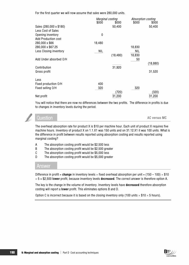
190 9: Marginal and absorption costing Part D Cost accounting techniques
For the first quarter we will now assume that sales were 280,000 units.
Marginal costing Absorption costing $000 $000 $000 $000
Sales (280,000 x $180) 50,400 50,400Less Cost of SalesOpening inventory 0Add Production cost280,000 x $66 18,480280,000 x $67.25 18,830Less Closing inventory NIL NIL
(18,480) 18,830Add Under absorbed O/H 50
(18,880)Contribution 31,920Gross profit 31,520
LessFixed production O/H 400Fixed selling O/H 320 320
(720) (320)Net profit 31,200 31,200
You will notice that there are now no differences between the two profits. The difference in profits is due to changes in inventory levels during the period.
Question AC versus MC
The overhead absorption rate for product X is $10 per machine hour. Each unit of product X requires five machine hours. Inventory of product X on 1.1.X1 was 150 units and on 31.12.X1 it was 100 units. What is the difference in profit between results reported using absorption costing and results reported using marginal costing?
A The absorption costing profit would be $2,500 less B The absorption costing profit would be $2,500 greater C The absorption costing profit would be $5,000 less D The absorption costing profit would be $5,000 greater
AnswerDifference in profit = change in inventory levels fixed overhead absorption per unit = (150 – 100) $10
5 = $2,500 lower profit, because inventory levels decreased. The correct answer is therefore option A.
The key is the change in the volume of inventory. Inventory levels have decreased therefore absorption costing will report a lower profit. This eliminates options B and D.
Option C is incorrect because it is based on the closing inventory only (100 units $10 5 hours).

Part D Cost accounting techniques 9: Marginal and absorption costing 191
4 Reconciling profits 4.1 Introduction
Reported profit figures using marginal costing or absorption costing will differ if there is any change in the level of inventories in the period. If production is equal to sales, there will be no difference in calculated profits using the costing methods.
The difference in profits reported under the two costing systems is due to the different inventory valuation methods used.
If inventory levels increase between the beginning and end of a period, absorption costing will report the higher profit. This is because some of the fixed production overhead incurred during the period will be carried forward in closing inventory (which reduces cost of sales) to be set against sales revenue in the following period instead of being written off in full against profit in the period concerned.
If inventory levels decrease, absorption costing will report the lower profit because as well as the fixed overhead incurred, fixed production overhead which had been carried forward in opening inventory is released and is also included in cost of sales.
4.2 Example: Reconciling profits The profits reported under absorption costing and marginal costing for January – March in the Big Woof question above can be reconciled as follows.
$’000Marginal costing profit 26,640Adjust for fixed overhead included in inventory: Inventory increase of 40,000 units $1.25 50Absorption costing profit 26,690
4.3 Reconciling profits – a shortcut A quick way to establish the difference in profits without going through the whole process of drawing up the income statements is as follows.
Difference in profits = change in inventory level x overhead absorption rate per unit
If inventory levels have gone up (that is, closing inventory > opening inventory) then absorption costingprofit will be greater than marginal costing profit.
If inventory levels have gone down (that is, closing inventory < opening inventory) then absorptioncosting profit will be less than marginal costing profit.
In the Big Woof example above
Change in inventory = 40,000 units (an increase)
Overhead absorption rate = $1.25 per unit
We would expect absorption costing profit to be greater than marginal costing profit by 40,000 x $1.25 = $50,000. If you check back to the answer, you will find that this is the case.
Question Absorption costing profit
When opening inventories were 8,500 litres and closing inventories 6,750 litres, a firm had a profit of $62,100 using marginal costing.
Assuming that the fixed overhead absorption rate was $3 per litre, what would be the profit using absorption costing?
A $41,850 B $56,850 C $67,350 D $82,350
FAST FORWARD

192 9: Marginal and absorption costing Part D Cost accounting techniques
AnswerDifference in profit = (8,500 – 6,750) $3 = $5,250
Absorption costing profit = $62,100 – $5,250 = $56,850
The correct answer is B.
Since inventory levels reduced, the absorption costing profit will be lower than the marginal costing profit. You can therefore eliminate options C and D.
Question Absorption versus marginal costing profits
Last month a manufacturing company’s profit was $2,000, calculated using absorption costing principles.If marginal costing principles has been used, a loss of $3,000 would have occurred. The company’s fixed production cost is $2 per unit. Sales last month were 10,000 units.
What was last month’s production (in units)?
A 7,500 B 9,500 C 10,500 D 12,500
AnswerThe correct answer is D.
Any difference between marginal and absorption costing profit is due to changes in inventory.$
Absorption costing profit 2,000 Marginal costing loss (3,000)Difference 5,000
Change in inventory = Difference in profit/fixed product cost per unit
= $5,000/$2 = 2,500 units
Marginal costing loss is lower than absorption costing profit therefore inventory has gone up – that is, production was greater than sales by 2,500 units.
Production = 10,000 units (sales) + 2,500 units = 12,500 units
The above question appeared in the December 2008 exam and was answered correctly by less than 50% of students. More than 40% of students selected B or C which probably meant that they had overlooked the fact that there was a marginal costing loss rather than a profit. This approach would have given an inventory change of 500 units.
The effect on profit of using the two different costing methods can be confusing. You must get it straight in your mind before the examination. Remember that if opening inventory values are greater than closing inventory values, marginal costing shows the greater profit.
Exam focus point

Part D Cost accounting techniques 9: Marginal and absorption costing 193
5 Marginal costing versus absorption costing
Absorption costing is most often used for routine profit reporting and must be used for financial accounting purposes. Marginal costing provides better management information for planning and decision making. There are a number of arguments both for and against each of the costing systems.
The following diagram summarises the arguments in favour of both marginal and absorption costing.
FAST FORWARD

194 9: Marginal and absorption costing Part D Cost accounting techniques
Chapter roundup
Marginal cost is the variable cost of one unit of product or service.
Contribution is an important measure in marginal costing, and it is calculated as the difference between sales value and marginal or variable cost of sales.
In marginal costing, fixed production costs are treated as period costs and are written off as they are incurred. In absorption costing, fixed production costs are absorbed into the cost of units and are carried forward in inventory to be charged against sales for the next period. Inventory values using absorption costing are therefore greater than those calculated using marginal costing.
Reported profit figures using marginal costing or absorption costing will differ if there is any change in the level of inventories in the period. If production is equal to sales, there will be no difference in calculated profits using these costing methods.
In your examination you may be asked to calculate the profit for an accounting period using either of the two methods of accounting. Absorption costing is most often used for routine profit reporting and must be used for financial accounting purposes. Marginal costing provides better management information for planning and decision making. There are a number of arguments both for and against each of the costing systems.
Quick quiz 1 What is marginal costing?
2 What is a period cost in marginal costing?
3 Sales value – marginal cost of sales = ………………….
4 What is a breakeven point?
5 Marginal costing and absorption costing are different techniques for assessing profit in a period. If there are changes in inventory during a period, marginal costing and absorption costing give different results for profit obtained.
Which of the following statements are true?
I If inventory levels increase, marginal costing will report the higher profit. II If inventory levels decrease, marginal costing will report the lower profit. III If inventory levels decrease, marginal costing will report the higher profit. IV If the opening and closing inventory volumes are the same, marginal costing and absorption
costing will give the same profit figure.
A All of the above C I and IV B I, II and IV D III and IV
6 Which of the following are arguments in favour of marginal costing?
(a) Closing stock (inventory) is valued in accordance with IAS 2. (b) It is simple to operate. (c) There is no under or over absorption of overheads. (d) Fixed costs are the same regardless of activity levels. (e) The information from this costing method may be used for decision making.

Part D Cost accounting techniques 9: Marginal and absorption costing 195
Answers to quick quiz 1 Marginal costing is an alternative method of costing to absorption costing. In marginal costing, only
variable costs are charged as a cost of sale and a contribution is calculated (sales revenue – variable cost of sales).
2 A fixed cost 3 Contribution 4 The point at which total contribution exactly equals fixed costs (no profit or loss is made) 5 D 6 (b), (c), (d), (e)
Now try the questions below from the Exam Question Bank
Number Level Marks Time
Q9 MCQ/OTQ n/a n/a

196 9: Marginal and absorption costing Part D Cost accounting techniques

197
Process costing
IntroductionIn this chapter we will consider process costing. The chapter will consider the topic from basics, looking at how to account for the most simple of processes. We then move on to how to account for any losses which might occur, as well as what to do with any scrapped units which are sold. We also consider how to deal with any closing work in progress and then look at two methods of valuing opening work in progress. Valuation of both opening and closing work in progress hinges on the concept of equivalent units, which will be explained in detail.
Topic list Syllabus reference
1 The basics of process costing D6 (a), (b), (c)
2 Losses in process costing D6 (d), (e)
3 Losses with scrap value D6 (e)
4 Losses with a disposal cost D6 (i)
5 Valuing closing work in progress D6 (f), (h)
6 Valuing opening work in progress: FIFO method D6 (g)
7 Valuing opening work in progress: weighted average cost method
D6 (g)

198 10: Process costing Part D Cost accounting techniques
Study guide Intellectual level
D6 Process costing
(a) Describe the characteristics of process costing 1
(b) Describe situations where the use of process costing would be appropriate 1
(c) Calculate the cost per unit of process outputs 1
(d) Explain the concepts of 'normal and abnormal' losses and 'abnormal' gains 1
(e) Prepare process accounts, involving normal and abnormal losses and abnormal gains
1
(f) Calculate and explain the concept of equivalent units 1
(g) Apportion process costs between work remaining in process and transfers out of a process using the weighted average and FIFO methods
2
(h) Prepare process accounts in situations where work remains incomplete 2
(i) Prepare process accounts where losses and gains are identified at different stages of the process
1
Note. Situations involving work in process and losses in the same process are excluded.
Exam guide Expect several questions on process costing. The pilot paper has four questions on this topic, and the examiner has stated that this is a good guide to the weighting of exam question topics in the exams for 2009-2010. The questions are shorter than the examples and questions in this chapter, but if you have worked through some long questions you will have covered whatever can come up in a short question.
1 The basics of process costing 1.1 Introduction to process costing
Process costing is a costing method used where it is not possible to identify separate units of production, or jobs, usually because of the continuous nature of the production processes involved.
It is common to identify process costing with continuous production such as the following.
Oil refining Foods and drinks Paper Chemicals
Process costing may also be associated with the continuous production of large volumes of low-cost items, such as cans or tins.
1.2 Features of process costing (a) The output of one process becomes the input to the next until the finished product is made in the
final process. (b) The continuous nature of production in many processes means that there will usually be closing work
in progress which must be valued. In process costing it is not possible to build up cost records of the cost per unit of output or the cost per unit of closing inventory because production in progress is an indistinguishable homogeneous mass.
(c) There is often a loss in process due to spoilage, wastage, evaporation and so on. (d) Output from production may be a single product, but there may also be a by-product (or by-
products) and/or joint products.
FAST FORWARD

Part D Cost accounting techniques 10: Process costing 199
The aim of this chapter is to describe how cost accountants keep a set of accounts to record the costs of production in a processing industry. The aim of the set of accounts is to derive a cost, or valuation, for output and closing inventory.
1.3 Process accounts Where a series of separate processes is required to manufacture the finished product, the output of one process becomes the input to the next until the final output is made in the final process. If two processes are required the accounts would look like this.
PROCESS 1 ACCOUNT
Units $ Units $Direct materials 1,000 50,000 Output to process 2 1,000 90,000Direct labour 20,000 Production overhead 20,000
1,000 90,000 1,000 90,000
PROCESS 2 ACCOUNT
Units $ Units $Materials from process 1 1,000 90,000 Output to finished goods 1,000 150,000Added materials 30,000 Direct labour 15,000 Production overhead 15,000
1,000 150,000 1,000 150,000
Note that direct labour and production overhead may be treated together in an examination question as conversion cost.
Added materials, labour and overhead in process 2 are added gradually throughout the process. Materials from process 1, in contrast, will often be introduced in full at the start of process 2.
The 'units' columns in the process accounts are for memorandum purposes only and help you to ensure that you do not miss out any entries.
1.4 Framework for dealing with process costing
Process costing is centred around four key steps. The exact work done at each step will depend on whether there are normal losses, scrap, opening and closing work in progress.
Step 1 Determine output and losses Step 2 Calculate cost per unit of output, losses and WIP Step 3 Calculate total cost of output, losses and WIP Step 4 Complete accounts
Let's look at these steps in more detail
Step 1 Determine output and losses. This step involves the following.
Determining expected output Calculating normal loss and abnormal loss and gain Calculating equivalent units if there is closing or opening work in progress
Step 2 Calculate cost per unit of output, losses and WIP. This step involves calculating cost per unit or cost per equivalent unit.
Step 3 Calculate total cost of output, losses and WIP. In some examples this will be straightforward; however in cases where there is closing and/or opening work-in-progress a statement of evaluation will have to be prepared.
Step 4 Complete accounts. This step involves the following.
Completing the process account Writing up the other accounts required by the question
FAST FORWARD
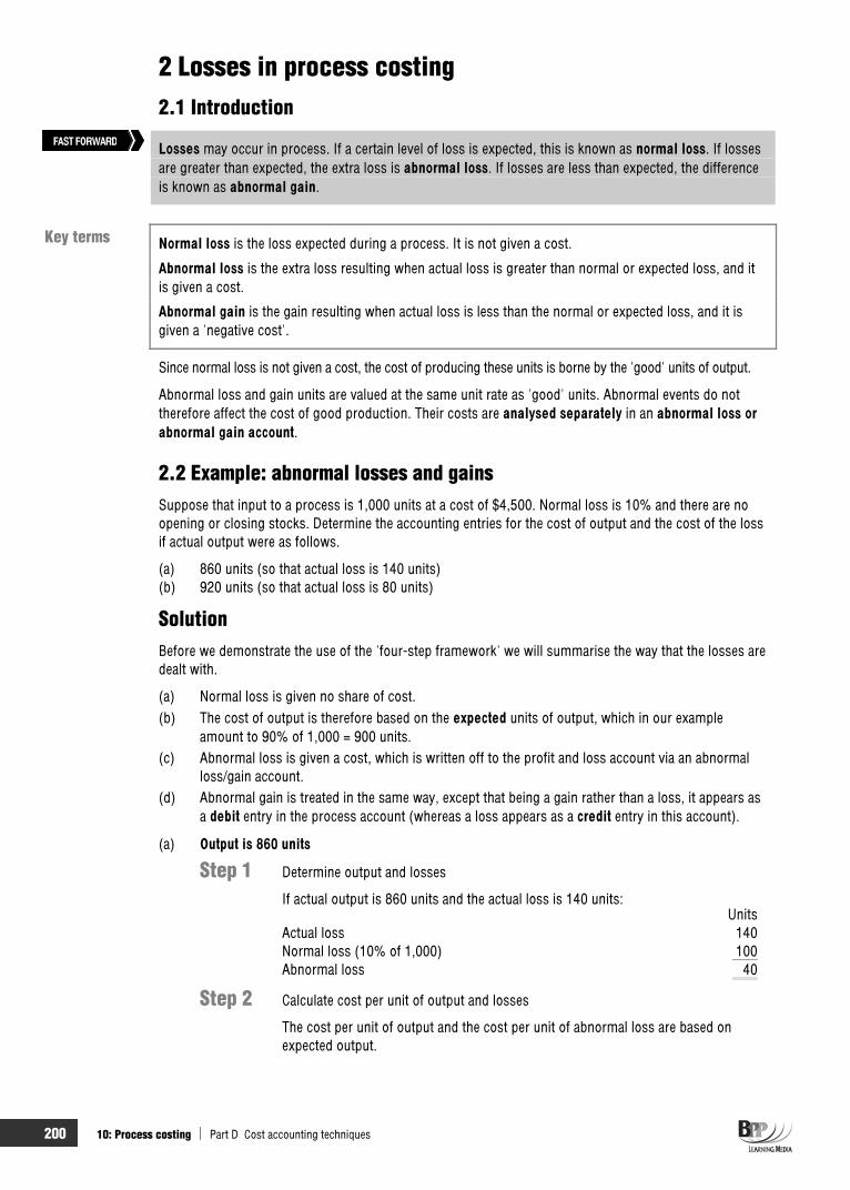
200 10: Process costing Part D Cost accounting techniques
2 Losses in process costing 2.1 Introduction
Losses may occur in process. If a certain level of loss is expected, this is known as normal loss. If losses are greater than expected, the extra loss is abnormal loss. If losses are less than expected, the difference is known as abnormal gain.
Normal loss is the loss expected during a process. It is not given a cost.
Abnormal loss is the extra loss resulting when actual loss is greater than normal or expected loss, and it is given a cost.
Abnormal gain is the gain resulting when actual loss is less than the normal or expected loss, and it is given a 'negative cost'.
Since normal loss is not given a cost, the cost of producing these units is borne by the 'good' units of output.
Abnormal loss and gain units are valued at the same unit rate as 'good' units. Abnormal events do not therefore affect the cost of good production. Their costs are analysed separately in an abnormal loss or abnormal gain account.
2.2 Example: abnormal losses and gains Suppose that input to a process is 1,000 units at a cost of $4,500. Normal loss is 10% and there are no opening or closing stocks. Determine the accounting entries for the cost of output and the cost of the loss if actual output were as follows.
(a) 860 units (so that actual loss is 140 units) (b) 920 units (so that actual loss is 80 units)
SolutionBefore we demonstrate the use of the 'four-step framework' we will summarise the way that the losses are dealt with.
(a) Normal loss is given no share of cost. (b) The cost of output is therefore based on the expected units of output, which in our example
amount to 90% of 1,000 = 900 units. (c) Abnormal loss is given a cost, which is written off to the profit and loss account via an abnormal
loss/gain account. (d) Abnormal gain is treated in the same way, except that being a gain rather than a loss, it appears as
a debit entry in the process account (whereas a loss appears as a credit entry in this account).
(a) Output is 860 units
Step 1 Determine output and losses
If actual output is 860 units and the actual loss is 140 units: Units
Actual loss 140Normal loss (10% of 1,000) 100Abnormal loss 40
Step 2 Calculate cost per unit of output and losses
The cost per unit of output and the cost per unit of abnormal loss are based on expected output.
Key terms
FAST FORWARD

Part D Cost accounting techniques 10: Process costing 201
output Expectedincurred Costs
=units900500,4$
= $5 per unit
Step 3 Calculate total cost of output and losses
Normal loss is not assigned any cost. $
Cost of output (860 $5) 4,300Normal loss 0Abnormal loss (40 $5) 200
4,500
Step 4 Complete accounts PROCESS ACCOUNT
Units $ Units $ Cost incurred 1,000 4,500 Normal loss 100 0
Output (finished goods a/c) 860 ( $5) 4,300
Abnormal loss 40 ( $5) 2001,000 4,500 1,000 4,500
ABNORMAL LOSS ACCOUNT
Units $ Units $ Process a/c 40 200 Income statement 40 200
(b) Output is 920 units
Step 1 Determine output and losses
If actual output is 920 units and the actual loss is 80 units: Units
Actual loss 80Normal loss (10% of 1,000) 100Abnormal gain 20
Step 2 Calculate cost per unit of output and losses
The cost per unit of output and the cost per unit of abnormal gain are based on expected output.
output Expectedincurred Costs
=units900
$4,500= $5 per unit
(Whether there is abnormal loss or gain does not affect the valuation of units of output. The figure of $5 per unit is exactly the same as in the previous paragraph, when there were 40 units of abnormal loss.)
Step 3 Calculate total cost of output and losses $
Cost of output (920 $5) 4,600Normal loss 0Abnormal gain (20 $5) (100)
4,500
Step 4 Complete accounts PROCESS ACCOUNT
Units $ Units $ Cost incurred 1,000 4,500 Normal loss 100 0 Abnormal gain a/c 20 (x $5) 100 Output 920 (x $5) 4,600
(finished goods a/c)1,020 4,600 1,020 4,600

202 10: Process costing Part D Cost accounting techniques
ABNORMAL GAIN
Units $ Units $ Income statement 20 100 Process a/c 20 100
Question Abnormal losses and gains
Shiny Co has two processes, Y and Z. There is an expected loss of 5% of input in process Y and 7% of input in process Z. Activity during a four week period is as follows.
Y Z Material input (kg) 20,000 28,000Output (kg) 18,500 26,100
Is there an abnormal gain or abnormal loss for each process?
Y ZA Abnormal loss Abnormal loss B Abnormal gain Abnormal loss C Abnormal loss Abnormal gain D Abnormal gain Abnormal gain
AnswerThe correct answer is C.
Y ZInput (kg) 20,000 28,000Normal loss (kg) 1,000 (5% of 20,000) 1,960 (7% of 28,000)Expected output 19,000 26,040Actual output 18,500 26,100Abnormal loss/gain 500 (loss) 60 (gain)
2.3 Example: Abnormal losses and gains again During a four-week period, period 3, costs of input to a process were $29,070. Input was 1,000 units, output was 850 units and normal loss is 10%.
During the next period, period 4, costs of input were again $29,070. Input was again 1,000 units, but output was 950 units.
There were no units of opening or closing inventory.
Required
Prepare the process account and abnormal loss or gain account for each period.
SolutionStep 1 Determine output and losses
Period 3 Units
Actual output 850Normal loss (10% 1,000) 100Abnormal loss 50Input 1,000

Part D Cost accounting techniques 10: Process costing 203
Period 4 Units
Actual output 950Normal loss (10% 1,000) 100Abnormal gain (50)Input 1,000
Step 2 Calculate cost per unit of output and losses
For each period the cost per unit is based on expected output.
output of units Expectedinput of Cost
= 900
070,29$ = $32.30 per unit
Step 3 Calculate total cost of output and losses
Period 3 $
Cost of output (850 $32.30) 27,455Normal loss 0Abnormal loss (50 $32.30) 1,615
29,070
Period 4 $
Cost of output (950 $32.30) 30,685Normal loss 0Abnormal gain (50 $32.30) 1,615
29,070
Step 4 Complete accounts PROCESS ACCOUNT
Units $ Units $Period 3 Cost of input 1,000 29,070 Normal loss 100 0 Finished goods a/c 850 27,455
( $32.30)Abnormal loss a/c 50 1,615( $32.30)
1,000 29,070 1,000 29,070Period 4 Cost of input 1,000 29,070 Normal loss 100 0Abnormal gain a/c 50 1,615 Finished goods a/c 950 30,685( $32.30) ( $32.30)
1,050 30,685 1,050 30,685
ABNORMAL LOSS OR GAIN ACCOUNT
$ $Period 3 Period 4 Abnormal loss in process a/c 1,615 Abnormal gain in process a/c 1,615
A nil balance on this account will be carried forward into period 5.
If there is a closing balance in the abnormal loss or gain account when the profit for the period is calculated, this balance is taken to the income statement: an abnormal gain will be a credit to the income statement and an abnormal loss will be a debit to the income statement.

204 10: Process costing Part D Cost accounting techniques
Question Process account
3,000 units of material are input to a process. Process costs are as follows.
Material $11,700 Conversion costs $6,300
Output is 2,000 units. Normal loss is 20% of input.
Required
Prepare a process account and the appropriate abnormal loss/gain account.
Answer
Step 1 Determine output and losses
We are told that output is 2,000 units. Normal loss = 20% 3,000 = 600 units Abnormal loss = (3,000 – 600) – 2,000 = 400 units
Step 2 Calculate cost per unit of output and losses
Cost per unit = 400,2
300,6700,11$ = $7.50
Step 3 Calculate total cost of output and losses$
Output (2,000 $7.50) 15,000Normal loss 0Abnormal loss (400 $7.50) 3,000
18,000
Step 4 Complete accountsPROCESS ACCOUNT
Units $ Units $Material 3,000 11,700 Output 2,000 15,000Conversion costs 6,300 Normal loss 600
Abnormal loss 400 3,0003,000 18,000 3,000 18,000
ABNORMAL LOSS ACCOUNT
$ $
Process a/c 3,000 Income statement 3,000
Question Finished output
Charlton Co manufactures a product in a single process operation. Normal loss is 10% of input. Loss occurs at the end of the process. Data for June are as follows.
Opening and closing inventories of work in progress Nil Cost of input materials (3,300 units) $59,100 Direct labour and production overhead $30,000 Output to finished goods 2,750 units
The full cost of finished output in June was
A $74,250 B $81,000 C $82,500 D $89,100

Part D Cost accounting techniques 10: Process costing 205
Answer
Step 1 Determine output and losses Units
Actual output 2,750Normal loss (10% 3,300) 330Abnormal loss 220
3,300
Step 2 Calculate cost per unit of output and losses
output of units Expectedinput of Cost
= 3303,300
$89,100 = $30 per unit
Step 3 Calculate total cost of output and losses $
Cost of output (2,750 $30) 82,500 (The correct answer is C)Normal loss 0Abnormal loss (220 $30) 6,600
89,100
If you were reduced to making a calculated guess, you could have eliminated option D. This is simply the total input cost, with no attempt to apportion some of the cost to the abnormal loss.
Option A is incorrect because it results from allocating a full unit cost to the normal loss: remember that normal loss does not carry any of the process cost.
Option B is incorrect because it results from calculating a 10% normal loss based on output of 2,750 units (275 units normal loss), rather than on input of 3,300 units.
3 Losses with scrap value
Scrap is 'Discarded material having some value.'
Loss or spoilage may have scrap value.
The scrap value of normal loss is usually deducted from the cost of materials.The scrap value of abnormal loss (or abnormal gain) is usually set off against its cost, in an abnormal loss (abnormal gain) account.
As the questions that follow will show, the three steps to remember are these.
Step 1 Separate the scrap value of normal loss from the scrap value of abnormal loss or gain.
Step 2 In effect, subtract the scrap value of normal loss from the cost of the process, by crediting it to the process account (as a 'value' for normal loss).
Key term
FAST FORWARD

206 10: Process costing Part D Cost accounting techniques
Step 3 Either subtract the value of abnormal loss scrap from the cost of abnormal loss, by crediting the abnormal loss account.
or subtract the cost of the abnormal gain scrap from the value of abnormal gain, by debiting the abnormal gain account.
Scrap value
Abnormal loss/gain Normal loss/gain
Deduct scrap value from cost of process i.e. Creditprocess account with scrap value of normal loss or normal gain
Deduct scrapvalue from cost of abnormal loss i.e. Credit abnormal loss account
Deduct scrapvalue from value of abnormal gain i.e. Debitabnormal gain account
LOSS GAIN
Question Losses and scrap
3,000 units of material are input to a process. Process costs are as follows.
Material $11,700 Conversion costs $6,300
Output is 2,000 units. Normal loss is 20% of input.
The units of loss could be sold for $1 each. Prepare appropriate accounts.
Answer
Step 1 Determine output and losses
Input 3,000 unitsNormal loss (20% of 3,000) 600 unitsExpected output 2,400 unitsActual output 2,000 unitsAbnormal loss 0 400 units
Step 2 Calculate cost per unit of output and losses $
Scrap value of normal loss 600Scrap value of abnormal loss 400Total scrap (1,000 units $1) 1,000
Cost per expected unit = 2,400
6,30060011,700$ = $7.25
Step 3 Calculate total cost of output and losses $
Output (2,000 $7.25) 14,500Normal loss (600 $1.00) 600Abnormal loss (400 $7.25) 2,900
18,000
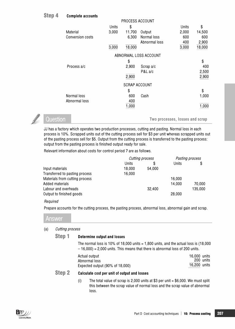
Part D Cost accounting techniques 10: Process costing 207
Step 4 Complete accounts PROCESS ACCOUNT
Units $ Units $Material 3,000 11,700 Output 2,000 14,500Conversion costs 6,300 Normal loss 600 600
Abnormal loss 400 2,9003,000 18,000 3,000 18,000
ABNORMAL LOSS ACCOUNT $ $
Process a/c 2,900 Scrap a/c 400P&L a/c 2,500
2,900 2,900
SCRAP ACCOUNT $ $
Normal loss 600 Cash 1,000Abnormal loss 400
1,000 1,000
Question Two processes, losses and scrap
JJ has a factory which operates two production processes, cutting and pasting. Normal loss in each process is 10%. Scrapped units out of the cutting process sell for $3 per unit whereas scrapped units out of the pasting process sell for $5. Output from the cutting process is transferred to the pasting process: output from the pasting process is finished output ready for sale.
Relevant information about costs for control period 7 are as follows.
Cutting process Pasting process Units $ Units $
Input materials 18,000 54,000 Transferred to pasting process 16,000Materials from cutting process 16,000 Added materials 14,000 70,000 Labour and overheads 32,400 135,000 Output to finished goods 28,000
Required
Prepare accounts for the cutting process, the pasting process, abnormal loss, abnormal gain and scrap.
Answer(a) Cutting process
Step 1 Determine output and losses
The normal loss is 10% of 18,000 units = 1,800 units, and the actual loss is (18,000 – 16,000) = 2,000 units. This means that there is abnormal loss of 200 units.
Actual output 16,000 units Abnormal loss 200 unitsExpected output (90% of 18,000) 16,200 units
Step 2 Calculate cost per unit of output and losses
(i) The total value of scrap is 2,000 units at $3 per unit = $6,000. We must split this between the scrap value of normal loss and the scrap value of abnormal loss.

208 10: Process costing Part D Cost accounting techniques
$ Normal loss (1,800 $3) 5,400Abnormal loss (200 $3) 600Total scrap (2,000 units $3) 6,000
(ii) The scrap value of normal loss is first deducted from the materials cost in the process, in order to calculate the output cost per unit and then credited to the process account as a 'value' for normal loss. The cost per unit in the cutting process is calculated as follows.
Cost per expectedTotal cost unit of output
$ $Materials 54,000Less normal loss scrap value* 5,400
48,600 ( 16,200) 3.00Labour and overhead 32,400 ( 16,200) 2.00Total 81,000 ( 16,200) 5.00
* It is usual to set this scrap value of normal loss against the cost of materials.
Step 3 Calculate total cost of output and losses $Output (16,000 units $5) 80,000Normal loss (1,800 units $3) 5,400Abnormal loss (200 units $5) 1,000
86,400
Step 4 Complete accounts
PROCESS 1 ACCOUNT
Units $ Units $Materials 18,000 54,000 Output to pasting process * 16,000 80,000Labour and Normal loss (scrap a/c) ** 1,800 5,400overhead 32,400 Abnormal loss a/c * 200 1,000
18,000 86,400 18,000 86,400
* At $5 per unit ** At $3 per unit
(b) Pasting process
Step 1 Determine output and losses
The normal loss is 10% of the units processed = 10% of (16,000 + 14,000) = 3,000 units. The actual loss is (30,000 – 28,000) = 2,000 units, so that there is abnormal gain of 1,000 units. These are deducted from actual output to determine expected output. Units Actual output 28,000Abnormal gain (1,000)Expected output (90% of 30,000) 27,000
Step 2 Calculate cost per unit of output and losses
(i) The total value of scrap is 2,000 units at $5 per unit = $10,000. We must split this between the scrap value of normal loss and the scrap value of abnormal gain. Abnormal gain's scrap value is 'negative'.
$Normal loss scrap value 3,000 units $5 15,000Abnormal gain scrap value 1,000 units $5 (5,000)Scrap value of actual loss 2,000 units $5 10,000
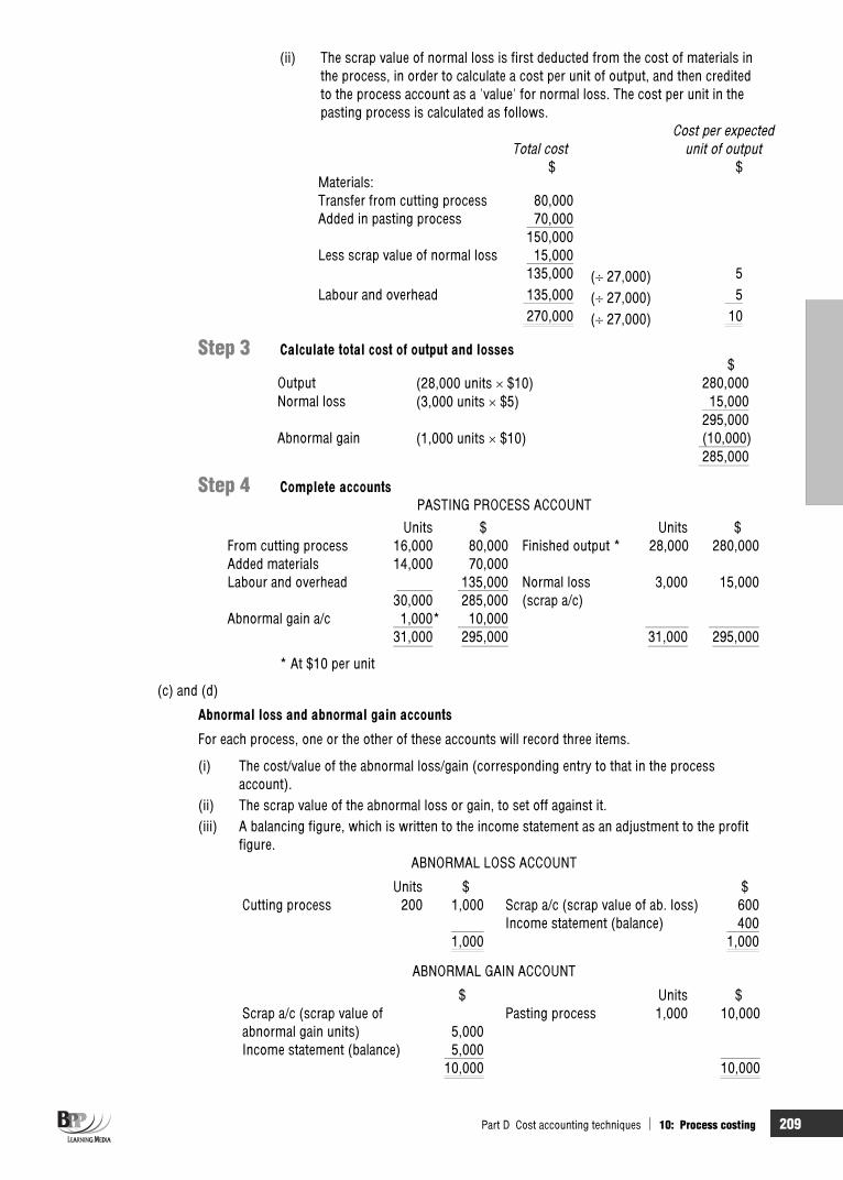
Part D Cost accounting techniques 10: Process costing 209
(ii) The scrap value of normal loss is first deducted from the cost of materials in the process, in order to calculate a cost per unit of output, and then credited to the process account as a 'value' for normal loss. The cost per unit in the pasting process is calculated as follows.
Total cost Cost per expected
unit of output $ $
Materials: Transfer from cutting process 80,000Added in pasting process 70,000
150,000Less scrap value of normal loss 15,000
135,000 ( 27,000) 5Labour and overhead 135,000 ( 27,000) 5
270,000 ( 27,000) 10
Step 3 Calculate total cost of output and losses$
Output (28,000 units $10) 280,000Normal loss (3,000 units $5) 15,000
295,000Abnormal gain (1,000 units $10) (10,000)
285,000
Step 4 Complete accounts PASTING PROCESS ACCOUNT
Units $ Units $From cutting process 16,000 80,000 Finished output * 28,000 280,000Added materials 14,000 70,000Labour and overhead 135,000 Normal loss 3,000 15,000
30,000 285,000 (scrap a/c) Abnormal gain a/c 1,000* 10,000
31,000 295,000 31,000 295,000
* At $10 per unit
(c) and (d)
Abnormal loss and abnormal gain accounts
For each process, one or the other of these accounts will record three items.
(i) The cost/value of the abnormal loss/gain (corresponding entry to that in the process account).
(ii) The scrap value of the abnormal loss or gain, to set off against it. (iii) A balancing figure, which is written to the income statement as an adjustment to the profit
figure. ABNORMAL LOSS ACCOUNT
Units $ $Cutting process 200 1,000 Scrap a/c (scrap value of ab. loss) 600
Income statement (balance) 4001,000 1,000
ABNORMAL GAIN ACCOUNT
$ Units $Scrap a/c (scrap value of Pasting process 1,000 10,000abnormal gain units) 5,000 Income statement (balance) 5,000
10,000 10,000
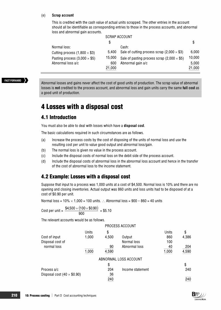
210 10: Process costing Part D Cost accounting techniques
(e) Scrap account
This is credited with the cash value of actual units scrapped. The other entries in the account should all be identifiable as corresponding entries to those in the process accounts, and abnormal loss and abnormal gain accounts.
SCRAP ACCOUNT$ $
Normal loss: Cash: Cutting process (1,800 $3) 5,400 Sale of cutting process scrap (2,000 $3) 6,000
Pasting process (3,000 $5) 15,000 Sale of pasting process scrap (2,000 $5) 10,000 Abnormal loss a/c 600 Abnormal gain a/c 5,000
21,000 21,000
Abnormal losses and gains never affect the cost of good units of production. The scrap value of abnormal losses is not credited to the process account, and abnormal loss and gain units carry the same full cost asa good unit of production.
4 Losses with a disposal cost 4.1 Introduction You must also be able to deal with losses which have a disposal cost.
The basic calculations required in such circumstances are as follows.
(a) Increase the process costs by the cost of disposing of the units of normal loss and use the resulting cost per unit to value good output and abnormal loss/gain.
(b) The normal loss is given no value in the process account. (c) Include the disposal costs of normal loss on the debit side of the process account. (d) Include the disposal costs of abnormal loss in the abnormal loss account and hence in the transfer
of the cost of abnormal loss to the income statement.
4.2 Example: Losses with a disposal cost Suppose that input to a process was 1,000 units at a cost of $4,500. Normal loss is 10% and there are no opening and closing inventories. Actual output was 860 units and loss units had to be disposed of at a cost of $0.90 per unit.
Normal loss = 10% 1,000 = 100 units. Abnormal loss = 900 – 860 = 40 units
Cost per unit = 900
90.0$100500,4$ = $5.10
The relevant accounts would be as follows.
PROCESS ACCOUNT
Units $ Units $Cost of input 1,000 4,500 Output 860 4,386Disposal cost of Normal loss 100 – normal loss 90 Abnormal loss 40 204
1,000 4,590 1,000 4,590
ABNORMAL LOSS ACCOUNT $ $
Process a/c 204 Income statement 240Disposal cost (40 $0.90) 36
240 240
FAST FORWARD

Part D Cost accounting techniques 10: Process costing 211
5 Valuing closing work in progress 5.1 Introduction
When units are partly completed at the end of a period (and hence there is closing work in progress), it is necessary to calculate the equivalent units of production in order to determine the cost of a completed unit.
The Study Guide states that losses and work in progress in the same process will not be examined.
In the examples we have looked at so far we have assumed that opening and closing inventories of work in process have been nil. We must now look at more realistic examples and consider how to allocate the costs incurred in a period between completed output (that is, finished units) and partly completed closing inventory.
Some examples will help to illustrate the problem, and the techniques used to share out (apportion) costs between finished output and closing inventories.
Suppose that we have the following account for Process 2 for period 9.
PROCESS ACCOUNT Units $ $
Materials 1,000 6,200 Finished goods 800 ?Labour and overhead 2,850 Closing WIP 200 ?
1,000 9,050 1,000 9,050
How do we value the finished goods and closing work in process?
With any form of process costing involving closing WIP, we have to apportion costs between output and closing WIP. To apportion costs 'fairly' we make use of the concept of equivalent units of production.
5.2 Equivalent units
Equivalent units are notional whole units which represent incomplete work, and which are used to apportion costs between work in process and completed output.
We will assume that in the example above the degree of completion is as follows.
(a) Direct materials. These are added in full at the start of processing, and so any closing WIP will have 100% of their direct material content. (This is not always the case in practice. Materials might be added gradually throughout the process, in which case closing inventory will only be a certain percentage complete as to material content. We will look at this later in the chapter.)
(b) Direct labour and production overhead. These are usually assumed to be incurred at an even rate through the production process, so that when we refer to a unit that is 50% complete, we mean that it is half complete for labour and overhead, although it might be 100% complete for materials.
Let us also assume that the closing WIP is 100% complete for materials and 25% complete for labour and overhead.
How would we now put a value to the finished output and the closing WIP?
In Step 1 of our framework, we have been told what output and losses are. However we also need to calculate equivalent units.
Key term
FAST FORWARD
Exam focus point

212 10: Process costing Part D Cost accounting techniques
STATEMENT OF EQUIVALENT UNITS Materials Labour and overhead Degree of Equivalent Degree of Equivalent Total units completion units completion units
Finished output 800 100% 800 100% 800Closing WIP 200 100% 200 25% 50
1,000 1,000 850
In Step 2 the important figure is average cost per equivalent unit. This can be calculated as follows.
STATEMENT OF COSTS PER EQUIVALENT UNIT Labour and
Materials overhead Costs incurred in the period $6,200 $2,850 Equivalent units of work done 1,000 850 Cost per equivalent unit (approx) $6.20 $3.3529
To calculate total costs for Step 3, we prepare a statement of evaluation to show how the costs should be apportioned between finished output and closing WIP.
STATEMENT OF EVALUATION
Materials Labour and overheads Cost per Cost per Equivalent equivalent Equivalent equivalent Total
Item units units Cost units units Cost cost $ $ $ $ $
Finished output 800 6.20 4,960 800 3.3529 2,682 7,642Closing WIP 200 6.20 1,240 50 3.3529 168 1,408
1,000 6,200 850 2,850 9,050
The process account (work in progress, or work in process account) would be shown as follows.
PROCESS ACCOUNT Units $ Units $
Materials 1,000 6,200 Finished goods 800 7,642Labour overhead 2,850 Closing WIP 200 1,408
1,000 9,050 1,000 9,050
Question Equivalent units for closing WIP
Ally Co has the following information available on Process 9.
PROCESS 9 ACCOUNT
$ $Input 10,000kg 59,150 Finished goods 8,000kg 52,000
Closing WIP 2,000kg 7,15059,150 59,150
How many equivalent units were there for Closing WIP?
A 1,000 C 2,000 B 1,100

Part D Cost accounting techniques 10: Process costing 213
AnswerThe correct answer is B.
This question requires you to work backwards. You can calculate the cost per unit using the Finished Goods figures.
Cost per unit = kg of Numbergoods finished of Cost
= 000,8000,52
= $6.50
If 2,000kg (Closing WIP figure) were fully complete total cost would be
2,000 x $6.50 = $13,000
Actual cost of Closing WIP = $7,150
Degree of completion = 000,13150,7
= 55%
Therefore equivalent units = 55% of 2,000 = 1,100kg
Question Equivalent units
Ashley Co operates a process costing system. The following details are available for Process 2.
Materials input at beginning of process 12,000 kg, costing $18,000 Labour and overheads added $28,000
10,000kg were completed and transferred to the Finished Goods account. The remaining units were 60% complete with regard to labour and overheads. There were no losses in the period.
What is the value of Closing WIP in the process account?
A $4,800 C $7,667 B $6,000 D $8,000
AnswerThe correct answer is B.
STATEMENT OF EQUIVALENT UNITS
Material LabourUnits Degree of Equivalent Units Degree of Equivalent
completion units completion unitsFinished goods 10,000 100% 10,000 10,000 100% 10,000Closing WIP 2,000 100% 2,000 2,000 60% 1,200
12,000 12,000 12,000 11,200
COSTS PER EQUIVALENT UNIT
Material LabourTotal cost $18,000 $28,000 Equivalent units 12,000 11,200 Cost per unit $1.50 $2.50
Total cost per unit = $4.00
Value of Closing WIP = ($1.50 x 2,000) + ($2.50 x 1,200) = $6,000
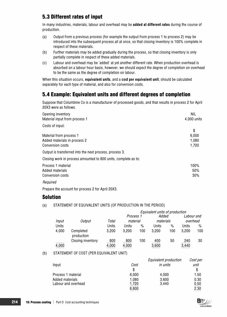
214 10: Process costing Part D Cost accounting techniques
5.3 Different rates of input In many industries, materials, labour and overhead may be added at different rates during the course of production.
(a) Output from a previous process (for example the output from process 1 to process 2) may be introduced into the subsequent process all at once, so that closing inventory is 100% complete in respect of these materials.
(b) Further materials may be added gradually during the process, so that closing inventory is only partially complete in respect of these added materials.
(c) Labour and overhead may be 'added' at yet another different rate. When production overhead is absorbed on a labour hour basis, however, we should expect the degree of completion on overhead to be the same as the degree of completion on labour.
When this situation occurs, equivalent units, and a cost per equivalent unit, should be calculated separately for each type of material, and also for conversion costs.
5.4 Example: Equivalent units and different degrees of completion Suppose that Columbine Co is a manufacturer of processed goods, and that results in process 2 for April 20X3 were as follows.
Opening inventory NIL Material input from process 1 4,000 units
Costs of input: $
Material from process 1 6,000 Added materials in process 2 1,080 Conversion costs 1,720
Output is transferred into the next process, process 3.
Closing work in process amounted to 800 units, complete as to:
Process 1 material 100% Added materials 50%Conversion costs 30%
Required
Prepare the account for process 2 for April 20X3.
Solution(a) STATEMENT OF EQUIVALENT UNITS (OF PRODUCTION IN THE PERIOD)
Equivalent units of production Process 1 Added Labour and
Input Output Total material materials overheadUnits Units Units % Units % Units %4,000 Completed 3,200 3,200 100 3,200 100 3,200 100
production Closing inventory 800 800 100 400 50 240 30
4,000 4,000 4,000 3,600 3,440
(b) STATEMENT OF COST (PER EQUIVALENT UNIT)
Equivalent production Cost per Input Cost in units unit
$ $Process 1 material 6,000 4,000 1.50Added materials 1,080 3,600 0.30Labour and overhead 1,720 3,440 0.50
8,800 2.30

Part D Cost accounting techniques 10: Process costing 215
(c) STATEMENT OF EVALUATION (OF FINISHED WORK AND CLOSING INVENTORIES)
Number of Cost per equivalent equivalent
Production Cost element units unit Total Cost$ $ $
Completed production 3,200 2.30 7,360Closing inventory: process 1 material 800 1.50 1,200
added material 400 0.30 120labour and overhead 240 0.50 120
1,4408,800
(d) PROCESS ACCOUNT Units $ Units $ Process 1 material 4,000 6,000 Process 3 a/c 3,200 7,360 Added material 1,080 Conversion costs 1,720 Closing inventory c/f 800 1,440
4,000 8,800 4,000 8,800
6 Valuing opening work in progress: FIFO method 6.1 Introduction
Account can be taken of opening work in progress using either the FIFO method or the weighted average cost method.
Opening work in progress is partly complete at the beginning of a period and is valued at the cost incurred to date. In the example in Paragraph 4.4, closing work in progress of 800 units at the end of April 20X3 would be carried forward as opening inventory, value $1,440, at the beginning of May 20X3.
It therefore follows that the work required to complete units of opening inventory is 100% minus the work in progress done in the previous period. For example, if 100 units of opening inventory are 70% complete at the beginning of June 20X2, the equivalent units of production would be as follows.
Equivalent units in previous period (May 20X2) (70%) = 70 Equivalent units to complete work in current period (June 20X2) (30%) = 30Total work done 100
The FIFO method of valuation deals with production on a first in, first out basis. The assumption is that the first units completed in any period are the units of opening inventory that were held at the beginning of the period.
6.2 Example: WIP and FIFO Suppose that information relating to process 1 of a two-stage production process is as follows, for August 20X2.
Opening inventory 500 units: degree of completion 60% Cost to date $2,800
Costs incurred in August 20X2 $ Direct materials (2,500 units introduced) 13,200 Direct labour 6,600 Production overhead 6,600
26,400
Closing inventory 300 units: degree of completion 80%
FAST FORWARD

216 10: Process costing Part D Cost accounting techniques
There was no loss in the process.
Required
Prepare the process 1 account for August 20X2.
SolutionAs the term implies, first in, first out means that in August 20X2 the first units completed were the units of opening inventory.
Opening inventories: work done to date = 60% plus work done in August 20X2 = 40%
The cost of the work done up to 1 August 20X2 is known to be $2,800, so that the cost of the units completed will be $2,800 plus the cost of completing the final 40% of the work on the units in August 20X2.
Once the opening inventory has been completed, all other finished output in August 20X2 will be work started as well as finished in the month.
UnitsTotal output in August 20X2 * 2,700Less opening inventory, completed first 500Work started and finished in August 20X2 2,200
(* Opening inventory plus units introduced minus closing inventory = 500 + 2,500 300)
What we are doing here is taking the total output of 2,700 units, and saying that we must divide it into two parts as follows.
(a) The opening inventory, which was first in and so must be first out. (b) The rest of the units, which were 100% worked in the period.
Dividing finished output into two parts in this way is a necessary feature of the FIFO valuation method.
Continuing the example, closing inventory of 300 units will be started in August 20X2, but not yet completed.
The total cost of output to process 2 during 20X2 will be as follows. $
Opening stock cost brought forward 2,800 (60%)plus cost incurred during August 20X2,to complete x (40%)
2,800 + xFully worked 2,200 units yTotal cost of output to process 2, FIFO basis 2,800 + x + y
Equivalent units will again be used as the basis for apportioning costs incurred during August 20X2. Be sure that you understand the treatment of 'opening inventory units completed', and can relate the calculations to the principles of FIFO valuation.
Step 1 Determine output and losses
STATEMENT OF EQUIVALENT UNITSEquivalent units of production
Total units in August 20X2Opening inventory unitscompleted
500 (40%) 200
Fully worked units 2,200 (100%) 2,200Output to process 2 2,700 2,400Closing inventory 300 (80%) 240
3,000 2,640
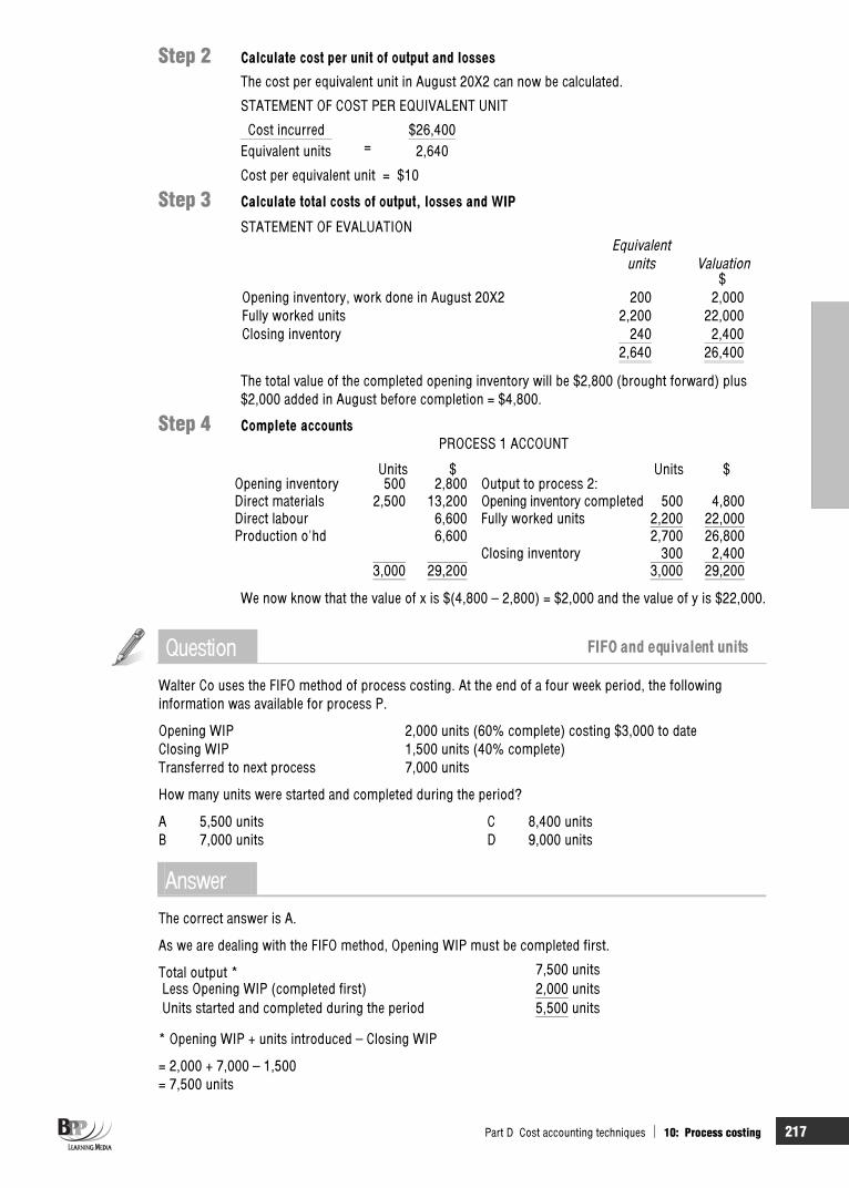
Part D Cost accounting techniques 10: Process costing 217
Step 2 Calculate cost per unit of output and losses
The cost per equivalent unit in August 20X2 can now be calculated.
STATEMENT OF COST PER EQUIVALENT UNIT
Cost incurred $26,400Equivalent units = 2,640
Cost per equivalent unit = $10
Step 3 Calculate total costs of output, losses and WIP
STATEMENT OF EVALUATION Equivalent
units Valuation$
Opening inventory, work done in August 20X2 200 2,000Fully worked units 2,200 22,000Closing inventory 240 2,400
2,640 26,400
The total value of the completed opening inventory will be $2,800 (brought forward) plus $2,000 added in August before completion = $4,800.
Step 4 Complete accounts PROCESS 1 ACCOUNT
Units $ Units $ Opening inventory 500 2,800 Output to process 2:Direct materials 2,500 13,200 Opening inventory completed 500 4,800Direct labour 6,600 Fully worked units 2,200 22,000Production o'hd 6,600 2,700 26,800
Closing inventory 300 2,4003,000 29,200 3,000 29,200
We now know that the value of x is $(4,800 – 2,800) = $2,000 and the value of y is $22,000.
Question FIFO and equivalent units
Walter Co uses the FIFO method of process costing. At the end of a four week period, the following information was available for process P.
Opening WIP 2,000 units (60% complete) costing $3,000 to date Closing WIP 1,500 units (40% complete) Transferred to next process 7,000 units
How many units were started and completed during the period?
A 5,500 units C 8,400 units B 7,000 units D 9,000 units
AnswerThe correct answer is A.
As we are dealing with the FIFO method, Opening WIP must be completed first.
Total output * 7,500 unitsLess Opening WIP (completed first) 2,000 unitsUnits started and completed during the period 5,500 units
* Opening WIP + units introduced – Closing WIP
= 2,000 + 7,000 – 1,500 = 7,500 units
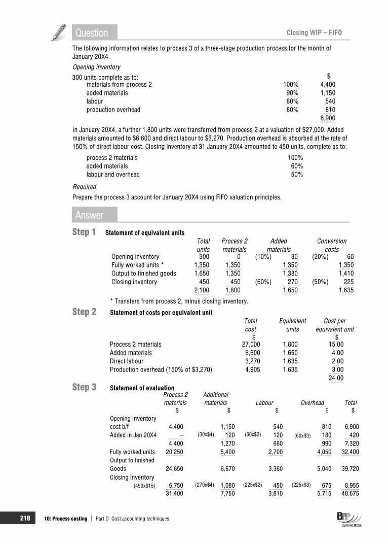
218 10: Process costing Part D Cost accounting techniques
Question Closing WIP – FIFO
The following information relates to process 3 of a three-stage production process for the month of January 20X4.
Opening inventory
300 units complete as to: $ materials from process 2 100% 4,400 added materials 90% 1,150 labour 80% 540 production overhead 80% 810
6,900
In January 20X4, a further 1,800 units were transferred from process 2 at a valuation of $27,000. Added materials amounted to $6,600 and direct labour to $3,270. Production overhead is absorbed at the rate of 150% of direct labour cost. Closing inventory at 31 January 20X4 amounted to 450 units, complete as to:
process 2 materials 100% added materials 60% labour and overhead 50%
Required
Prepare the process 3 account for January 20X4 using FIFO valuation principles.
Answer
Step 1 Statement of equivalent units Total Process 2 Added Conversion units materials materials costs
Opening inventory 300 0 (10%) 30 (20%) 60Fully worked units * 1,350 1,350 1,350 1,350Output to finished goods 1,650 1,350 1,380 1,410Closing inventory 450 450 (60%) 270 (50%) 225
2,100 1,800 1,650 1,635
* Transfers from process 2, minus closing inventory.
Step 2 Statement of costs per equivalent unitTotal Equivalent Cost percost units equivalent unit
$ $Process 2 materials 27,000 1,800 15.00Added materials 6,600 1,650 4.00Direct labour 3,270 1,635 2.00Production overhead (150% of $3,270) 4,905 1,635 3.00
24.00Step 3 Statement of evaluation
Process 2 Additional materials materials Labour Overhead Total
$ $ $ $ $Opening inventorycost b/f 4,400 1,150 540 810 6,900Added in Jan 20X4 – (30x$4) 120 (60x$2) 120 (60x$3) 180 420
4,400 1,270 660 990 7,320Fully worked units 20,250 5,400 2,700 4,050 32,400Output to finishedGoods 24,650 6,670 3,360 5,040 39,720 Closing inventory
(450x$15) 6,750 (270x$4) 1,080 (225x$2) 450 (225x$3) 675 8,95531,400 7,750 3,810 5,715 48,675

Part D Cost accounting techniques 10: Process costing 219
Step 4 Complete accountsPROCESS 3 ACCOUNT
Units $ Units $ Opening inventory b/f 300 6,900 Finished goods a/c 1,650 39,720 Process 2 a/c 1,800 27,000 Stores a/c 6,600 Wages a/c 3,270 Production o'hd a/c 4,905 Closing inventory c/f 450 8,955
2,100 48,675 2,100 48,675
Question Equivalent units and FIFO
Cheryl Co operates a FIFO process costing system. The following information is available for last month.
Opening work in progress 2,000 units valued at $3,000Input 60,000 units costing $30,000
Conversion costs $20,000Units transferred to next process 52,000 units Closing work in progress 10,000 units
Opening work in progress was 100% complete with regard to input materials and 70% complete as to conversion. Closing work in progress was complete with regard to input materials and 80% complete as to conversion.
What was the number of equivalent units with regard to conversion costs?
A 44,000 C 52,000 B 50,600 D 58,600
AnswerThe correct answer is D.
Units
Opening work in progress 30% of 2,000 units still to be completed 600Closing work in progress 80% of 10,000 units completed 8,000Units started and completed (Opening WIP + input – closing WIP) – opening WIP 50,000
58,600
7 Valuing opening work in progress: weighted average cost method
7.1 Introduction An alternative to FIFO is the weighted average cost method of inventory valuation which calculates a weighted average cost of units produced from both opening inventory and units introduced in the current period.
By this method no distinction is made between units of opening inventory and new units introduced tothe process during the accounting period. The cost of opening inventory is added to costs incurred during the period, and completed units of opening inventory are each given a value of one full equivalent unit of production.

220 10: Process costing Part D Cost accounting techniques
7.2 Example: Weighted average cost methodMagpie produces an item which is manufactured in two consecutive processes. Information relating to process 2 during September 20X3 is as follows.
Opening inventory 800 units Degree of completion: $
process 1 materials 100% 4,700added materials 40% 600conversion costs 30% 1,000
6,300
During September 20X3, 3,000 units were transferred from process 1 at a valuation of $18,100. Added materials cost $9,600 and conversion costs were $11,800.
Closing inventory at 30 September 20X3 amounted to 1,000 units which were 100% complete with respect to process 1 materials and 60% complete with respect to added materials. Conversion cost work was 40% complete.
Magpie uses a weighted average cost system for the valuation of output and closing inventory.
Required
Prepare the process 2 account for September 20X3.
SolutionStep 1 Opening inventory units count as a full equivalent unit of production when the weighted
average cost system is applied. Closing inventory equivalent units are assessed in the usual way.
STATEMENT OF EQUIVALENT UNITS Equivalent units
Total Process 1 Added Conversionunits material material costs
Opening inventory 800 (100%) 800 800 800Fully worked units* 2,000 (100%) 2,000 2,000 2,000Output to finished goods 2,800 2,800 2,800 2,800Closing inventory 1,000 (100%) 1,000 (60%) 600 (40%) 400
3,800 3,800 3,400 3,200
(*3,000 units from process 1 minus closing inventory of 1,000 units)
Step 2 The cost of opening inventory is added to costs incurred in September 20X3, and a cost per equivalent unit is then calculated.
STATEMENT OF COSTS PER EQUIVALENT UNIT
Process 1 Added Conversion material materials costs $ $ $ Opening inventory 4,700 600 1,000 Added in September 20X3 18,100 9,600 11,800Total cost 22,800 10,200 12,800
Equivalent units 3,800 units 3,400 units 3,200 units Cost per equivalent unit $6 $3 $4

Part D Cost accounting techniques 10: Process costing 221
Step 3 STATEMENT OF EVALUATION Process 1 Added Conversion Total
material materials costs cost$ $ $ $
Output to finished goods (2,800 units) 16,800 8,400 11,200 36,400 Closing inventory 6,000 1,800 1,600 9,400 45,800
Step 4 PROCESS 2 ACCOUNT Units $ Units $
Opening inventory b/f 800 6,300 Finished goods a/c 2,800 36,400 Process 1 a/c 3,000 18,100 Added materials 9,600 Conversion costs 11,800 Closing inventory c/f 1,000 9,400
3,800 45,800 3,800 45,800
7.3 Which method should be used? FIFO inventory valuation is more common than the weighted average method, and should be used unless an indication is given to the contrary. You may find that you are presented with limited information about the opening inventory, which forces you to use either the FIFO or the weighted average method. The rules are as follows.
(a) If you are told the degree of completion of each element in opening inventory, but not the value of each cost element, then you must use the FIFO method.
(b) If you are not given the degree of completion of each cost element in opening inventory, but you are given the value of each cost element, then you must use the weighted average method.
Question Equivalent units
During August, a factory commenced work on 20,000 units. At the start of the month there were no partly finished units but at the end of the month there were 2,000 units which were only 40% complete. Costs in the month were $3,722,400.
(a) How many equivalent units of closing WIP were there in the month?
A 20,000 C 18,000 B 2,000 D 800
(b) What is the total value of fully completed output which would show in the process account?
A $3,960,000 C $3,722,400 B $3,564,000 D $3,350,160
Answer(a) D Equivalent units of WIP = 40% 2,000 = 800
(b) B Total finished output 18,000 units
Total equivalent units = 18,000 100% 18,000 2,000 40% 800
18,800
Cost per equivalent unit = 3,722,400/18,800 = $198
Value of fully completed output: 18,000 198 = $3,564,000
222 10: Process costing Part D Cost accounting techniques
Chapter roundup
Process costing is a costing method used where it is not possible to identify separate units of production or jobs, usually because of the continuous nature of the production processes involved.
Process costing is centred around four key steps. The exact work done at each step will depend on whether there are normal losses, scrap, opening and closing work in progress.
Step 1. Determine output and losses Step 2. Calculate cost per unit of output, losses and WIP Step 3. Calculate total cost of output, losses and WIP Step 4. Complete accounts
Losses may occur in process. If a certain level of loss is expected, this is known as normal loss. If losses are greater than expected, the extra loss is abnormal loss. If losses are less than expected, the difference is known as abnormal gain.
The scrap value of normal loss is usually deducted from the cost of materials.
The scrap value of abnormal loss (or abnormal gain) is usually set off against its cost, in an abnormal loss (abnormal gain) account
Abnormal losses and gains never affect the cost of good units of production. The scrap value of abnormal loss is not credited to the process account, and abnormal loss and gain units carry the same full cost as a good unit of production.
When units are partly completed at the end of a period (and hence there is closing work in progress), it is necessary to calculate the equivalent units of production in order to determine the cost of a completed unit.
Account can be taken of opening work in progress using either the FIFO method or the weighted average cost method.
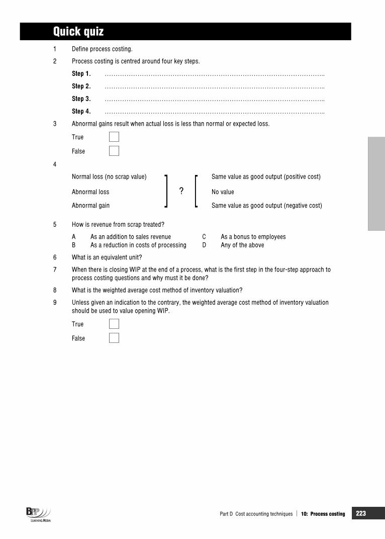
Part D Cost accounting techniques 10: Process costing 223
Quick quiz 1 Define process costing.
2 Process costing is centred around four key steps.
Step 1. ………………………………………………………………………………………..
Step 2. ………………………………………………………………………………………..
Step 3. ………………………………………………………………………………………..
Step 4. ………………………………………………………………………………………..
3 Abnormal gains result when actual loss is less than normal or expected loss.
True
False
4
Normal loss (no scrap value) Same value as good output (positive cost)
Abnormal loss ? No value
Abnormal gain Same value as good output (negative cost)
5 How is revenue from scrap treated?
A As an addition to sales revenue C As a bonus to employees B As a reduction in costs of processing D Any of the above
6 What is an equivalent unit?
7 When there is closing WIP at the end of a process, what is the first step in the four-step approach to process costing questions and why must it be done?
8 What is the weighted average cost method of inventory valuation?
9 Unless given an indication to the contrary, the weighted average cost method of inventory valuation should be used to value opening WIP.
True
False

224 10: Process costing Part D Cost accounting techniques
Answers to quick quiz 1 Process costing is a costing method used where it is not possible to identify separate units of production,
or jobs, usually because of the continuous nature of the production processes involved.
2 Step 1. Determine output and losses Step 2. Calculate cost per unit of output, losses and WIP Step 3. Calculate total cost of output, losses and WIP Step 4. Complete accounts
3 True
4
Normal loss (no scrap value) Same value as good output (positive cost)
Abnormal loss No value
Abnormal gain Same value as good output (negative cost)
5 B
6 An equivalent unit is a notional whole unit which represents incomplete work, and which is used to apportion costs between work in process and completed output.
7 Step 1. It is necessary to calculate the equivalent units of production (by drawing up a statement of equivalent units). Equivalent units of production are notional whole units which represent incomplete work and which are used to apportion costs between work in progress and completed output.
8 A method where no distinction is made between units of opening inventory and new units introduced to the process during the current period.
9 False. FIFO inventory valuation is more common than the weighted average method and should be used unless an indication is given to the contrary.
Now try the questions below from the Exam Question Bank
Number Level Marks Time
Q10 MCQ/OTQ n/a n/a

225
Process costing,joint products and by-products
IntroductionYou should now be aware of the most simple and the more complex areas of process costing. In this chapter we are going to turn our attention to the methods of accounting for joint products and by-products which arise as a result of a continuous process.
Topic list Syllabus reference
1 Joint products and by-products D6 (j)
2 Dealing with common costs D6 (k)
3 Joint products in process accounts D6 (l)
4 Accounting for by-products D6 (l)
226 11: Process costing, joint products and by-products Part D Cost accounting techniques
Study guide Intellectual level
D6 Process costing 2
(a) Distinguish between by-products and joint products 1
(b) Value by-products and joint products at the point of separation 1
(c) Prepare process accounts in situations where by-products and/or joint products occur
2
Exam guide The F2 Pilot paper has four questions on process costing, so make sure you understand all the basics here.
1 Joint products and by-products 1.1 Introduction
Joint products are two or more products separated in a process, each of which has a significant valuecompared to the other. A by-product is an incidental product from a process which has an insignificantvalue compared to the main product.
Joint products are two or more products which are output from the same processing operation, but which are indistinguishable from each other up to their point of separation.
A by-product is a supplementary or secondary product (arising as the result of a process) whose value is small relative to that of the principal product.
(a) Joint products have a substantial sales value. Often they require further processing before they are ready for sale. Joint products arise, for example, in the oil refining industry where diesel fuel, petrol, paraffin and lubricants are all produced from the same process.
(b) The distinguishing feature of a by-product is its relatively low sales value in comparison to the main product. In the timber industry, for example, by-products include sawdust, small offcuts and bark.
What exactly separates a joint product from a by-product?
(a) A joint product is regarded as an important saleable item, and so it should be separately costed.The profitability of each joint product should be assessed in the cost accounts.
(b) A by-product is not important as a saleable item, and whatever revenue it earns is a 'bonus' for the organisation. Because of their relative insignificance, by-products are not separately costed.
The study guide for Paper F2 states that you must be able to 'distinguish between by-products and joint products'.
1.2 Problems in accounting for joint products
The point at which joint products and by-products become separately identifiable is known as the split-offpoint or separation point. Costs incurred up to this point are called common costs or joint costs.
Key terms
Exam focus point
FAST FORWARD
FAST FORWARD

Part D Cost accounting techniques 11: Process costing, joint products and by-products 227
Costs incurred prior to this point of separation are common or joint costs, and these need to be allocated (apportioned) in some manner to each of the joint products. In the following sketched example, there are two different split-off points.
Problems in accounting for joint products are basically of two different sorts.
(a) How common costs should be apportioned between products, in order to put a value to closing inventories and to the cost of sale (and profit) for each product.
(b) Whether it is more profitable to sell a joint product at one stage of processing, or to process the product further and sell it at a later stage.
2 Dealing with common costs 2.1 Introduction
The main methods of apportioning joint costs, each of which can produce significantly different results are as follows.
Physical measurement Relative sales value apportionment method; sales value at split-off point
The problem of costing for joint products concerns common costs, that is those common processing costs shared between the units of eventual output up to their 'split-off point'. Some method needs to be devised for sharing the common costs between the individual joint products for the following reasons.
(a) To put a value to closing inventories of each joint product. (b) To record the costs and therefore the profit from each joint product. (c) Perhaps to assist in pricing decisions.
Here are some examples of the common costs problem.
(a) How to spread the common costs of oil refining between the joint products made (petrol, naphtha, kerosene and so on).
(b) How to spread the common costs of running the telephone network between telephone calls in peak and cheap rate times, or between local and long distance calls.
Various methods that might be used to establish a basis for apportioning or allocating common costs to each product are as follows.
Physical measurement Relative sales value apportionment method; sales value at split-off point
2.2 Dealing with common costs: physical measurement With physical measurement, the common cost is apportioned to the joint products on the basis of the proportion that the output of each product bears by weight or volume to the total output. An example of this would be the case where two products, product 1 and product 2, incur common costs to the point of separation of $3,000 and the output of each product is 600 tons and 1,200 tons respectively.
FAST FORWARD

228 11: Process costing, joint products and by-products Part D Cost accounting techniques
Product 1 sells for $4 per ton and product 2 for $2 per ton.
The division of the common costs ($3,000) between product 1 and product 2 could be based on the tonnage of output.
Product 1 Product 2 Total Output 600 tons + 1,200 tons 1,800 tons
Proportion of common cost 800,1600 +
800,1200,1
$ $ $ Apportioned cost 1,000 2,000 3,000Sales 2,400 2,400 4,800Profit 1,400 400 1,800
Profit/sales ratio 58.3% 16.7% 37.5%
Physical measurement has the following limitations.
(a) Where the products separate during the processes into different states, for example where one product is a gas and another is a liquid, this method is unsuitable.
(b) This method does not take into account the relative income-earning potentials of the individual products, with the result that one product might appear very profitable and another appear to be incurring losses.
2.3 Dealing with common costs: sales value at split-off point
The relative sales value method is the most widely used method of apportioning joint costs because (ignoring the effect of further processing costs) it assumes that all products achieve the same profit margin.
With relative sales value apportionment of common costs, the cost is allocated according to the product's ability to produce income. This method is most widely used because the assumption that some profit margin should be attained for all products under normal marketing conditions is satisfied. The common cost is apportioned to each product in the proportion that the sales (market) value of that product bears to the sales value of the total output from the particular processes concerned. Using the previous example where the sales price per unit is $4 for product 1 and $2 for product 2.
(a) Common costs of processes to split-off point $3,000 (b) Sales value of product 1 at $4 per ton $2,400 (c) Sales value of product 2 at $2 per ton $2,400
Product 1 Product 2 TotalSales $2,400 $2,400 $4,800
Proportion of common cost apportioned 800,4400,2
800,4400,2
FAST FORWARD

Part D Cost accounting techniques 11: Process costing, joint products and by-products 229
$ $ $ Apportioned cost 1,500 1,500 3,000 Sales 2,400 2,400 4,800Profit 900 900 1,800
Profit/sales ratio 37.5% 37.5% 37.5%
A comparison of the gross profit margin resulting from the application of the above methods for allocating common costs will illustrate the greater acceptability of the relative sales value apportionment method. Physical measurement gives a higher profit margin to product 1, not necessarily because product 1 is highly profitable, but because it has been given a smaller share of common costs.
Question Joint products
In process costing, a joint product is
A A product which is produced simultaneously with other products but which is of lesser value than at least one of the other products
B A product which is produced simultaneously with other products and is of similar value to at least one of the other products
C A product which is produced simultaneously with other products but which is of greater value than any of the other products
D A product produced jointly with another organisation
AnswerThe correct answer is B, a product which is of similar value to at least one of the other products.
Question Sales value method
Two products (W and X) are created from a joint process. Both products can be sold immediately after split-off. There are no opening inventories or work in progress. The following information is available for last period.
Total joint production costs $776,160
Product Production units Sales units Selling price per unit W 12,000 10,000 $10 X 10,000 8,000 $12
Using the sales value method of apportioning joint production costs, what was the value of the closing inventory of product X for last period?
A $68,992 B $70,560 C $76,032 D $77,616
AnswerThe correct answer is D.
Sales value of production:
Product W (12,000 x $10) $120,000 Product X (10,000 x $12) $120,000
Therefore joint costs are apportioned in the ratio 1:1.

230 11: Process costing, joint products and by-products Part D Cost accounting techniques
Amount apportioned to product X (776,160/2) $388,080
20% of X’s production is in closing inventory = 20% of $388,080 = $77,616
The above question is taken from the December 2007 exam. It was highlighted by the examiner as being poorly answered, with less than 30% of students selecting the correct answer. Make sure you split the joint costs according to sales value of production rather than individual selling prices or sales value of sales.
3 Joint products in process accounts This example illustrates how joint products are incorporated into process accounts.
3.1 Example: joint products and process accounts Three joint products are manufactured in a common process, which consists of two consecutive stages. Output from process 1 is transferred to process 2, and output from process 2 consists of the three joint products, Hans, Nils and Bumpsydaisies. All joint products are sold as soon as they are produced.
Data for period 2 of 20X6 are as follows.
Process 1 Process 2 Opening and closing inventory None NoneDirect material(30,000 units at $2 per unit) $60,000 –Conversion costs $76,500 $226,200Normal loss 10% of input 10% of input Scrap value of normal loss $0.50 per unit $2 per unit Output 26,000 units 10,000 units of Han
7,000 units of Nil 6,000 units of Bumpsydaisy
Selling prices are $18 per unit of Han, $20 per unit of Nil and $30 per unit of Bumpsydaisy.
Required
(a) Prepare the Process 1 account. (b) Prepare the Process 2 account using the sales value method of apportionment. (c) Prepare a profit statement for the joint products.
Solution(a) Process 1 equivalent units
Total Equivalent units unitsOutput to process 2 26,000 26,000 Normal loss 3,000 0Abnormal loss (balance) 1,000 1,000
30,000 27,000Costs of process 1
$Direct materials 60,000 Conversion costs 76,500
136,500Less scrap value of normal loss (3,000 $0.50) 1,500
135,000
Exam focus point
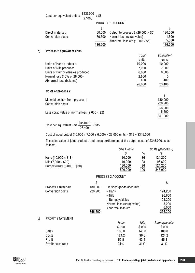
Part D Cost accounting techniques 11: Process costing, joint products and by-products 231
Cost per equivalent unit = 000,27
000,135$ = $5
PROCESS 1 ACCOUNT
$ $Direct materials 60,000 Output to process 2 (26,000 $5) 130,000Conversion costs 76,500 Normal loss (scrap value) 1,500
Abnormal loss a/c (1,000 $5) 5,000136,500 136,500
(b) Process 2 equivalent units Total Equivalent units unitsUnits of Hans produced 10,000 10,000 Units of Nils produced 7,000 7,000 Units of Bumpsydaisies produced 6,000 6,000 Normal loss (10% of 26,000) 2,600 0Abnormal loss (balance) 400 400
26,000 23,400
Costs of process 2 $
Material costs – from process 1 130,000Conversion costs 226,200
356,200Less scrap value of normal loss (2,600 $2) 5,200
351,000
Cost per equivalent unit 400,23000,351$
= $15
Cost of good output (10,000 + 7,000 + 6,000) = 23,000 units $15 = $345,000
The sales value of joint products, and the apportionment of the output costs of $345,000, is as follows.
Sales value Costs (process 2) $ % $
Hans (10,000 $18) 180,000 36 124,200 Nils (7,000 $20) 140,000 28 96,600 Bumpsydaisy (6,000 $30) 180,000 36 124,200
500,000 100 345,000
PROCESS 2 ACCOUNT
$ $Process 1 materials 130,000 Finished goods accounts Conversion costs 226,200 – Hans 124,200
– Nils 96,600 – Bumpsydaisies 124,200
Normal loss (scrap value) 5,200 Abnormal loss a/c 6,000
356,200 356,200
(c) PROFIT STATEMENT Hans Nils Bumpsydaisies
$'000 $'000 $'000Sales 180.0 140.0 180.0Costs 124.2 96.6 124.2Profit 55.8 43.4 55.8Profit/ sales ratio 31% 31% 31%

232 11: Process costing, joint products and by-products Part D Cost accounting techniques
Question Unit basis of apportionment
Prepare the Process 2 account and a profit statement for the joint products in the above example using the units basis of apportionment.
AnswerPROCESS 2 ACCOUNT
$ $Process 1 materials 130,000 Finished goods accounts Conversion costs 226,200 – Hans (10,000 $15) 150,000
– Nils (7,000 $15) 105,000– Bumpsydaisies (6,000 $15) 90,000
Normal loss (scrap value) 5,200 Abnormal loss a/c 6,000
356,200 356,200
PROFIT STATEMENT Hans Nils Bumpsydaisies $'000 $'000 $'000Sales 180 140 180Costs 150 105 90Profit 30 35 90Profit/ sales ratio 16.7% 25% 50%
Question Joint costs and process costing
Polly Co operates a process costing system, the final output from which is three different products: Bolly, Dolly and Folly. Details of the three products for March are as follows.
Bolly Dolly Folly Selling price per unit $25 $18 $32Output for March 6,000 units 10,000 units 4,000 units
22,000 units of material were input to the process, costing $242,000. Conversion costs were $121,000. No losses were expected and there were no opening or closing inventories.
Using the units basis of apportioning joint costs, what was the profit or loss on sales of Dolly for March?
A $(1,500) C $50,306 B $30,000 D $15,000
AnswerThe correct answer is D.
Total output 20,000 units (6,000 + 10,000 + 4,000)Total input 22,000 unitsAbnormal loss 2,000 units
Total cost = $363,000
Cost per unit = 000,22
000,363$ = $16.50
Cost of 'good' output = 20,000 units $16.50 = $330,000
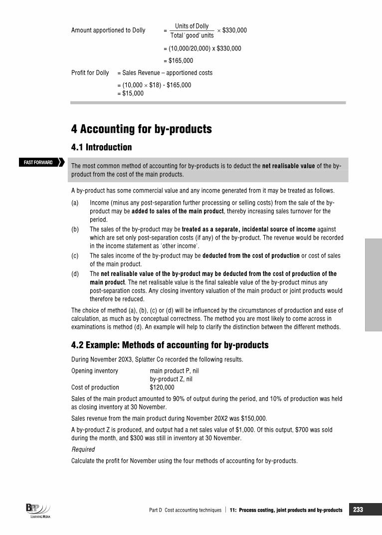
Part D Cost accounting techniques 11: Process costing, joint products and by-products 233
Amount apportioned to Dolly = units good'' Total
DollyofUnits $330,000
= (10,000/20,000) x $330,000
= $165,000
Profit for Dolly = Sales Revenue – apportioned costs
= (10,000 $18) - $165,000 = $15,000
4 Accounting for by-products 4.1 Introduction
The most common method of accounting for by-products is to deduct the net realisable value of the by-product from the cost of the main products.
A by-product has some commercial value and any income generated from it may be treated as follows.
(a) Income (minus any post-separation further processing or selling costs) from the sale of the by-product may be added to sales of the main product, thereby increasing sales turnover for the period.
(b) The sales of the by-product may be treated as a separate, incidental source of income against which are set only post-separation costs (if any) of the by-product. The revenue would be recorded in the income statement as 'other income'.
(c) The sales income of the by-product may be deducted from the cost of production or cost of sales of the main product.
(d) The net realisable value of the by-product may be deducted from the cost of production of the main product. The net realisable value is the final saleable value of the by-product minus any post-separation costs. Any closing inventory valuation of the main product or joint products would therefore be reduced.
The choice of method (a), (b), (c) or (d) will be influenced by the circumstances of production and ease of calculation, as much as by conceptual correctness. The method you are most likely to come across in examinations is method (d). An example will help to clarify the distinction between the different methods.
4.2 Example: Methods of accounting for by-productsDuring November 20X3, Splatter Co recorded the following results.
Opening inventory main product P, nil by-product Z, nil Cost of production $120,000
Sales of the main product amounted to 90% of output during the period, and 10% of production was held as closing inventory at 30 November.
Sales revenue from the main product during November 20X2 was $150,000.
A by-product Z is produced, and output had a net sales value of $1,000. Of this output, $700 was sold during the month, and $300 was still in inventory at 30 November.
Required
Calculate the profit for November using the four methods of accounting for by-products.
FAST FORWARD

234 11: Process costing, joint products and by-products Part D Cost accounting techniques
SolutionThe four methods of accounting for by-products are shown below.
(a) Income from by-product added to sales of the main product $ $
Sales of main product ($150,000 + $700) 150,700 Opening inventory 0Cost of production 120,000 120,000 Less closing inventory (10%) 12,000Cost of sales 108,000Profit, main product 42,700
The closing inventory of the by-product has no recorded value in the cost accounts.
(b) By-product income treated as a separate source of income$ $
Sales, main product 150,000 Opening inventory 0Cost of production 120,000 120,000 Closing inventory (10%) 12,000Cost of sales, main product 108,000Profit, main product 42,000 Other income 700Total profit 42,700
The closing inventory of the by-product again has no value in the cost accounts.
(c) Sales income of the by-product deducted from the cost of production in the period
$ $Sales, main product 150,000 Opening inventory 0Cost of production (120,000 700) 119,300 119,300 Less closing inventory (10%) 11,930Cost of sales 107,370Profit, main product 42,630
Although the profit is different from the figure in (a) and (b), the by-product closing inventory again has no value.
(d) Net realisable value of the by-product deducted from the cost of production in the period
$ $Sales, main product 150,000 Opening inventory 0Cost of production (120,000 1,000) 119,000 119,000 Less closing inventory (10%) 11,900Cost of sales 107,100Profit, main product 42,900
As with the other three methods, closing inventory of the by-product has no value in the books of accounting, but the value of the closing inventory ($300) has been used to reduce the cost of production, and in this respect it has been allowed for in deriving the cost of sales and the profit for the period.

Part D Cost accounting techniques 11: Process costing, joint products and by-products 235
Question Profits
Randolph manufactures two joint products, J and K, in a common process. A by-product X is also produced. Data for the month of December 20X2 were as follows.
Opening inventories nilCosts of processing direct materials $25,500 direct labour $10,000
Production overheads are absorbed at the rate of 300% of direct labour costs. Production Sales Units UnitsOutput and sales consisted of: product J 8,000 7,000 product K 8,000 6,000 by-product X 1,000 1,000
The sales value per unit of J, K and X is $4, $6 and $0.50 respectively. The saleable value of the by-product is deducted from process costs before apportioning costs to each joint product. Costs of the common processing are apportioned between product J and product K on the basis of sales value of production.
The individual profits for December 20X2 are:
Product J Product K $ $ A 5,250 6,750 B 6,750 5,250 C 22,750 29,250 D 29,250 22,750
AnswerThe sales value of production was $80,000.
$ Product J (8,000 $4) 32,000 (40%)Product K (8,000 $6) 48,000 (60%)
80,000
The costs of production were as follows. $ Direct materials 25,500 Direct labour 10,000 Overhead (300% of $10,000) 30,000
65,500Less sales value of by-product (1,000 50c) 500Net production costs 65,000
The profit statement would appear as follows (nil opening inventories). Product J Product K Total
$ $ $ Production costs (40%) 26,000 (60%) 39,000 65,000 Less closing inventory (see working below)
(1,000 units) 3,250 (2,000 units) 9,750 13,000
Cost of sales 22,750 29,250 52,000 Sales (7,000 units) 28,000 (6,000 units) 36,000 64,000Profit 5,250 6,750 12,000
Working
Closing inventory = (Production units – sales units) x (production costs/production units)
For J, closing inventory = (8,000 – 7,000) x ($26,000/8,000) = $3,250
For K, closing inventory = (8,000 – 6,000) x ($39,000/8,000) = $9,750

236 11: Process costing, joint products and by-products Part D Cost accounting techniques
The correct answer is therefore A.
If you selected option B, you got the profits for each product mixed up.
If you selected option C or D, you calculated the cost of sales instead of the profit.
Chapter roundup
Joint products are two or more products separated in a process, each of which has a significant value compared to the other. A by-product is an incidental product from a process which has an insignificantvalue compared to the main product.
The point at which joint and by-products become separately identifiable is known as the split-off point or separation point. Costs incurred up to this point are called common costs or joint costs.
The main methods of apportioning joint costs, each of which can produce significantly different results are as follows: physical measurement; and relative sales value apportionment method; sales value at split-off point
The relative sales value method is the most widely used method of apportioning joint costs because (ignoring the effect of further processing costs) it assumes that all products achieve the same profit margin.
The most common method of accounting for by-products is to deduct the net realisable value of the by-product from the cost of the main products.
Quick quiz 1 What is the difference between a joint product and a by-product? 2 What is meant by the term 'split-off' point? 3 Name two methods of apportioning common costs to joint products. 4 Describe the four methods of accounting for by-products.
Answers to quick quiz 1 A joint product is regarded as an important saleable item whereas a by-product is not. 2 The split-off point (or the separation point) is the point at which joint products become separately
identifiable in a processing operation. 3 Physical measurement and sales value at split-off point. 4 See paragraph 4.1.
Now try the questions below from the Exam Question Bank
Number Level Marks Time
Q11 MCQ n/a n/a
237
Job, batch and service costing
IntroductionThe first costing method that we shall be looking at is job costing. We will see the circumstances in which job costing should be used and how the costs of jobs are calculated. We will look at how the costing of individual jobs fits in with the recording of total costs in control accounts and then we will move on to batch costing, the procedure for which is similar to job costing.
Service costing deals with specialist services supplied to third parties or an internal service supplied within an organisation.
Topic list Syllabus reference
1 Costing methods D5 (a)
2 Job costing D5 (a), (b), (c), (d)
3 Batch costing D5 (a), (b), (c), (d)
4 Service costing D7(a), (b), (c)
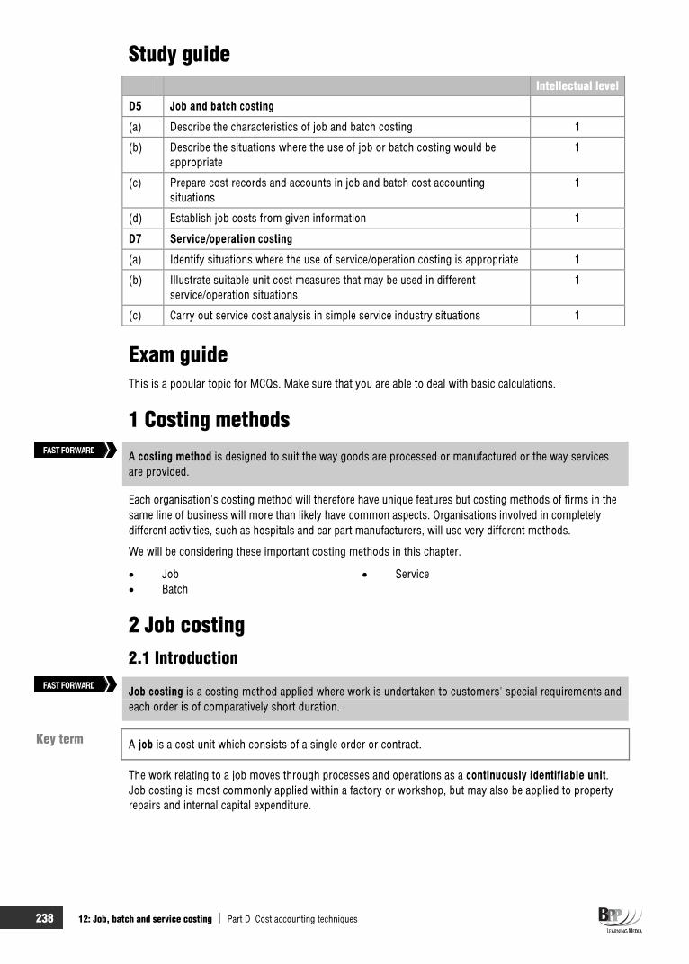
238 12: Job, batch and service costing Part D Cost accounting techniques
Study guide Intellectual level
D5 Job and batch costing
(a) Describe the characteristics of job and batch costing 1
(b) Describe the situations where the use of job or batch costing would be appropriate
1
(c) Prepare cost records and accounts in job and batch cost accounting situations
1
(d) Establish job costs from given information 1
D7 Service/operation costing
(a) Identify situations where the use of service/operation costing is appropriate 1
(b) Illustrate suitable unit cost measures that may be used in different service/operation situations
1
(c) Carry out service cost analysis in simple service industry situations 1
Exam guide This is a popular topic for MCQs. Make sure that you are able to deal with basic calculations.
1 Costing methods
A costing method is designed to suit the way goods are processed or manufactured or the way services are provided.
Each organisation's costing method will therefore have unique features but costing methods of firms in the same line of business will more than likely have common aspects. Organisations involved in completely different activities, such as hospitals and car part manufacturers, will use very different methods.
We will be considering these important costing methods in this chapter.
Job Service Batch
2 Job costing 2.1 Introduction
Job costing is a costing method applied where work is undertaken to customers' special requirements and each order is of comparatively short duration.
A job is a cost unit which consists of a single order or contract.
The work relating to a job moves through processes and operations as a continuously identifiable unit.Job costing is most commonly applied within a factory or workshop, but may also be applied to property repairs and internal capital expenditure.
Key term
FAST FORWARD
FAST FORWARD

Part D Cost accounting techniques 12: Job, batch and service costing 239
2.2 Procedure for the performance of jobs The normal procedure in jobbing concerns involves:
(a) The prospective customer approaches the supplier and indicates the requirements of the job. (b) A representative sees the prospective customer and agrees with him the precise details of the
items to be supplied. For example the quantity, quality, size and colour of the goods, the date of delivery and any special requirements.
(c) The estimating department of the organisation then prepares an estimate for the job. This will be based on the cost of the materials to be used, the labour expense expected, the cost overheads, the cost of any additional equipment needed specially for the job, and finally the supplier's profitmargin. The total of these items will represent the quoted selling price.
(d) If the estimate is accepted the job can be scheduled. All materials, labour and equipment required will be 'booked' for the job. In an efficient organisation, the start of the job will be timed to ensure that while it will be ready for the customer by the promised date of delivery it will not be loaded too early, otherwise storage space will have to be found for the product until the date it is required by (and was promised to) the customer.
2.3 Job cost sheets/cards
Costs for each job are collected on a job cost sheet or job card.
With other methods of costing, it is usual to produce for inventory; this means that management must decide in advance how many units of each type, size, colour, quality and so on will be produced during the coming year, regardless of the identity of the customers who will eventually buy the product. In job costing, because production is usually carried out in accordance with the special requirements of each customer, it is usual for each job to differ in one or more respects from another job.
A separate record must therefore be maintained to show the details of individual jobs. Such records are often known as job cost sheets or job cost cards. An example is shown on the next page.
Either the detail of relatively small jobs or a summary of direct materials, direct labour and so on forlarger jobs will be shown on a job cost sheet.
2.4 Job cost information
Material costs for each job are determined from material requisition notes. Labour times on each job are recorded on a job ticket, which is then costed and recorded on the job cost sheet. Some labour costs, such as overtime premium or the cost of rectifying sub-standard output, might be charged either directly to a job or else as an overhead cost, depending on the circumstances in which the costs have arisen. Overhead is absorbed into the cost of jobs using the predetermined overhead absorption rates.
Information for the direct and indirect costs will be gathered as follows.
2.4.1 Direct material cost
(a) The estimated cost will be calculated by valuing all items on the bill of materials. Materials that have to be specially purchased for the job in question will need to be priced by the purchasing department.
(b) The actual cost of materials used will be calculated by valuing materials issues notes for those issues from store for the job and/or from invoices for materials specially purchased. All documentation should indicate the job number to which it relates.
FAST FORWARD
FAST FORWARD

240 12: Job, batch and service costing Part D Cost accounting techniques
2.4.2 Direct labour cost
(a) The estimated labour time requirement will be calculated from past experience of similar types of work or work study engineers may prepare estimates following detailed specifications. Labour rates will need to take account of any increases, overtime and bonuses.
(b) The actual labour hours will be available from either time sheets or job tickets/cards, using job numbers where appropriate to indicate the time spent on each job. The actual labour cost will be calculated using the hours information and current labour rates (plus bonuses, overtime payments and so on).
2.4.3 Direct expenses
(a) The estimated cost of any expenses likely to be incurred can be obtained from a supplier. (b) The details of actual direct expenses incurred can be taken from invoices.
Part D Cost accounting techniques 12: Job, batch and service costing 241
2.4.4 Production overheads
(a) The estimated production overheads to be included in the job cost will be calculated from overhead absorption rates in operation and the estimate of the basis of the absorption rate (for example, direct labour hours). This assumes the job estimate is to include overheads (in a competitive environment management may feel that if overheads are to be incurred irrespective of whether or not the job is taken on, the minimum estimated quotation price should be based on variable costs only).
(b) The actual production overhead to be included in the job cost will be calculated from the overhead absorption rate and the actual results (such as labour hours coded to the job in question). Inaccurate overhead absorption rates can seriously harm an organisation; if jobs are over priced, customers will go elsewhere and if jobs are under priced revenue will fail to cover costs.
2.4.5 Administration, selling and distribution overheads
The organisation may absorb non-production overheads using any one of a variety of methods (percentage on full production cost, for example) and estimates of these costs and the actual costs should be included in the estimated and actual job cost.
2.5 Rectification costs If the finished output is found to be sub-standard, it may be possible to rectify the fault. The sub-standard output will then be returned to the department or cost centre where the fault arose.
Rectification costs can be treated in two ways.
(a) If rectification work is not a frequent occurrence, but arises on occasions with specific jobs to which it can be traced directly, then the rectification costs should be charged as a direct cost to the jobs concerned.
(b) If rectification is regarded as a normal part of the work carried out generally in the department, then the rectification costs should be treated as production overheads. This means that they would be included in the total of production overheads for the department and absorbed into the cost of all jobs for the period, using the overhead absorption rate.
2.6 Work in progress At the year end, the value of work in progress is simply the sum of the costs incurred on incomplete jobs(provided that the costs are lower than the net realisable value of the customer order).
2.7 Pricing the job
The usual method of fixing prices in a jobbing concern is cost plus pricing.
Cost plus pricing means that a desired profit margin is added to total costs to arrive at the selling price.
The estimated profit will depend on the particular circumstance of the job and organisation in question. In competitive situations the profit may be small but if the organisation is sure of securing the job the margin may be greater. In general terms, the profit earned on each job should conform to the requirements of the organisation's overall business plan.
The final price quoted will, of course, be affected by what competitors charge and what the customer will be willing to pay.
FAST FORWARD

242 12: Job, batch and service costing Part D Cost accounting techniques
An exam question about job costing may ask you to accumulate costs to arrive at a job cost, and then to determine a job price by adding a certain amount of profit. To do this, you need to remember the following crucial formula.
%Cost of job 100+ profit 25= selling price 125
Profit may be expressed either as a percentage of job cost (such as 25% (25/100) mark up) or as a percentage of selling price (such as 20% (25/125) margin).
2.8 Job costing and computerisation Job cost sheets exist in manual systems, but it is increasingly likely that in large organisations the jobcosting system will be computerised, using accounting software specifically designed to deal with job costing requirements. A computerised job accounting system is likely to contain the following features.
(a) Every job will be given a job code number, which will determine how the data relating to the job is stored.
(b) A separate set of codes will be given for the type of costs that any job is likely to incur. Thus, 'direct wages', say, will have the same code whichever job they are allocated to.
(c) In a sophisticated system, costs can be analysed both by job (for example all costs related to Job 456), but also by type (for example direct wages incurred on all jobs). It is thus easy to perform control analysis and to make comparisons between jobs.
(d) A job costing system might have facilities built into it which incorporate other factors relating to the performance of the job. In complex jobs, sophisticated planning techniques might be employed to ensure that the job is performed in the minimum time possible: time management features may be incorporated into job costing software.
2.9 Example: Job costing Fateful Morn is a jobbing company. On 1 June 20X2, there was one uncompleted job in the factory. The job card for this work is summarised as follows.
Job Card, Job No 6832 Costs to date $ Direct materials 630 Direct labour (120 hours) 350 Factory overhead ($2 per direct labour hour) 240Factory cost to date 1,220
During June, three new jobs were started in the factory, and costs of production were as follows.
Direct materials $Issued to: Job 6832 2,390 Job 6833 1,680 Job 6834 3,950 Job 6835 4,420Damaged inventory written off from stores 2,300
Material transfers $Job 6834 to Job 6833 250Job 6832 to 6834 620
Materials returned to store $From Job 6832 870From Job 6835 170
Exam focus point

Part D Cost accounting techniques 12: Job, batch and service costing 243
Direct labour hours recorded Job 6832 430 hrs Job 6833 650 hrs Job 6834 280 hrs Job 6835 410 hrs
The cost of labour hours during June 20X2 was $3 per hour, and production overhead is absorbed at the rate of $2 per direct labour hour. Production overheads incurred during the month amounted to $3,800. Completed jobs were delivered to customers as soon as they were completed, and the invoiced amounts were as follows.
Job 6832 $5,500Job 6834 $8,000Job 6835 $7,500
Administration and marketing overheads are added to the cost of sales at the rate of 20% of factory cost. Actual costs incurred during June 20X2 amounted to $3,200.
Required
(a) Prepare the job accounts for each individual job during June 20X2; (the accounts should only show the cost of production, and not the full cost of sale).
(b) Prepare the summarised job cost cards for each job, and calculate the profit on each completed job.
Solution(a) Job accounts
JOB 6832
$ $Balance b/f 1,220 Job 6834 a/c 620Materials (stores a/c) 2,390 (materials transfer) Labour (wages a/c) 1,290 Stores a/c (materials returned) 870 Production overhead (o'hd a/c) 860 Cost of sales a/c (balance) 4,270
5,760 5,760
JOB 6833
$ $Materials (stores a/c) 1,680 Balance c/f 5,180Labour (wages a/c) 1,950 Production overhead (o'hd a/c) 1,300 Job 6834 a/c (materials transfer) 250
5,180 5,180
JOB 6834
$ $Materials (stores a/c) 3,950 Job 6833 a/c (materials transfer) 250 Labour (wages a/c) 840 Production overhead (o'hd a/c) 560 Cost of sales a/c (balance) 5,720 Job 6832 a/c (materials transfer) 620
5,970 5,970
JOB 6835
$ $Materials (stores a/c) 4,420 Stores a/c (materials returned) 170 Labour (wages a/c) 1,230 Production overhead (o'hd a/c) 820 Cost of sales a/c (balance) 6,300
6,470 6,470

244 12: Job, batch and service costing Part D Cost accounting techniques
(b) Job cards, summarisedJob 6832 Job 6833 Job 6834 Job 6835
$ $ $ $Materials 1,530* 1,930 4,320** 4,250Labour 1,640 1,950 840 1,230Production overhead 1,100 1,300 560 820Factory cost 4,270 5,180 (c/f) 5,720 6,300Admin & marketing o'hd (20%) 854 1,144 1,260Cost of sale 5,124 6,864 7,560Invoice value 5,500 8,000 7,500Profit/(loss) on job 376 1,136 (60)
*$(630 + 2,390 – 620 – 870) **$(3,950 + 620 – 250)
2.10 Job costing for internal services
It is possible to use a job costing system to control the costs of an internal service department, such as the maintenance department or the printing department.
If a job costing system is used it is possible to charge the user departments for the cost of specific jobs carried out, rather than apportioning the total costs of these service departments to the user departments using an arbitrarily determined apportionment basis.
An internal job costing system for service departments will have the following advantages.
Advantages Comment
Realisticapportionment
The identification of expenses with jobs and the subsequent charging of these to the department(s) responsible means that costs are borne by those who incurred them.
Increasedresponsibility and awareness
User departments will be aware that they are charged for the specific services used and may be more careful to use the facility more efficiently. They will also appreciate the true cost of the facilities that they are using and can take decisions accordingly.
Control of service department costs
The service department may be restricted to charging a standard cost to user departments for specific jobs carried out or time spent. It will then be possible to measure the efficiency or inefficiency of the service department by recording the difference between the standard charges and the actual expenditure.
Planning information This information will ease the planning process, as the purpose and cost of service department expenditure can be separately identified.
Question Total job cost
A furniture-making business manufactures quality furniture to customers' orders. It has three production departments (A, B and C) which have overhead absorption rates (per direct labour hour) of $12.86, $12.40 and $14.03 respectively.
Two pieces of furniture are to be manufactured for customers. Direct costs are as follows.
Job XYZ Job MNO Direct material $154 $108Direct labour 20 hours dept A 16 hours dept A
12 hours dept B 10 hours dept B 10 hours dept C 14 hours dept C
Labour rates are as follows: $3.80(A); $3.50 (B); $3.40 (C)
FAST FORWARD

Part D Cost accounting techniques 12: Job, batch and service costing 245
Calculate the total cost of each job.
AnswerJob XYZ Job MNO
$ $Direct material 154.00 108.00Direct labour: dept A (20 3.80) 76.00 (16 3.80) 60.80 dept B (12 3.50) 42.00 (10 3.50) 35.00 dept C (10 3.40) 34.00 (14 3.40) 47.60Total direct cost 306.00 251.40Overhead: dept A (20 12.86) 257.20 (16 12.86) 205.76 dept B (12 12.40) 148.80 (10 12.40) 124.00 dept C (10 14.03) 140.30 (14 14.03) 196.42Total cost 852.30 777.58
Question Closing work in progress
A firm uses job costing and recovers overheads on direct labour.
Three jobs were worked on during a period, the details of which are as follows.
Job 1 Job 2 Job 3 $ $ $
Opening work in progress 8,500 0 46,000 Material in period 17,150 29,025 0Labour for period 12,500 23,000 4,500
The overheads for the period were exactly as budgeted, $140,000.
Jobs 1 and 2 were the only incomplete jobs.
What was the value of closing work in progress?
A $81,900 B $90,175 C $140,675 D $214,425
AnswerTotal labour cost = $12,500 + $23,000 + $4,500 = $40,000
Overhead absorption rate = 000,40$000,140$
100% = 350% of direct labour cost
Closing work in progress valuation Job 1 Job 2 Total
$ $ $Costs given in question 38,150 52,025 90,175Overhead absorbed (12,500 350%) 43,750 (23,000 350%) 80,500 124,250 214,425
Option D is correct.
We can eliminate option B because $90,175 is simply the total of the costs allocated to Jobs 1 and 2, with no absorption of overheads. Option A is an even lower cost figure, therefore it can also be eliminated.
Option C is wrong because it is a simple total of all allocated costs, including Job 3 which is not incomplete.

246 12: Job, batch and service costing Part D Cost accounting techniques
3 Batch costing 3.1 Introduction
Batch costing is similar to job costing in that each batch of similar articles is separately identifiable. The cost per unit manufactured in a batch is the total batch cost divided by the number of units in the batch.
A batch is a group of similar articles which maintains its identity during one or more stages of production and is treated as a cost unit.
In general, the procedures for costing batches are very similar to those for costing jobs.
(a) The batch is treated as a job during production and the costs are collected in the manner already described in this chapter.
(b) Once the batch has been completed, the cost per unit can be calculated as the total batch cost divided into the number of units in the batch.
3.2 Example: Batch costing Rio manufactures Brazils to order and has the following budgeted overheads for the year, based on normal activity levels.
Production departments Budgeted Overheads Budgeted activity $
Welding 12,000 3,000 labour hours Assembly 20,000 2,000 labour hours
Selling and administrative overheads are 25% of factory cost. An order for 500 Brazils, made as Batch 38, incurred the following costs.
Materials $24,000
Labour 200 hours in the Welding Department at $5 per hour 400 hours in the Assembly Department at $10 per hour
$1,000 was paid for the hire of x-ray equipment for testing the accuracy of the welds.
Required
Calculate the cost per unit for Batch 38.
SolutionThe first step is to calculate the overhead absorption rate for the production departments.
Welding = 000,3
000,12$ = $4 per labour hour
Assembly = 000,2
000,20$ = $10 per labour hour
Key term
FAST FORWARD

Part D Cost accounting techniques 12: Job, batch and service costing 247
Total cost – Batch 38$ $
Direct material 24,000Direct expense 1,000Direct labour 200 $5 = 1,000
400 $10 = 4,000 5,000
Prime cost 30,000Overheads 200 $4 = 800
400 $10 = 4,000 4,800
Factory cost 34,800Selling and administrative cost (25% of factory cost) 8,700Total cost 43,500
Cost per unit =500
500,43$ = $87
4 Service costing 4.1 What is service costing?
Service costing can be used by companies operating in a service industry or by companies wishing to establish the cost of services carried out by some of their departments. Service organisations do not make or sell tangible goods.
Service costing (or function costing) is a costing method concerned with establishing the costs, not of items of production, but of services rendered.
Service costing is used in the following circumstances.
(a) A company operating in a service industry will cost its services, for which sales revenue will be earned; examples are electricians, car hire services, road, rail or air transport services and hotels.
(b) A company may wish to establish the cost of services carried out by some of its departments; for example the costs of the vans or lorries used in distribution, the costs of the computer department, or the staff canteen.
4.2 Service costing versus product costing (such as job or process costing) (a) With many services, the cost of direct materials consumed will be relatively small compared to the
labour, direct expenses and overheads cost. In product costing the direct materials are often a greater proportion of the total cost.
(b) Although many services are revenue-earning, others are not (such as the distribution facility or the staff canteen). This means that the purpose of service costing may not be to establish a profit or loss (nor to value closing inventories for the balance sheet) but may rather be to provide management information about the comparative costs or efficiency of the services, with a view to helping managers to budget for their costs using historical data as a basis for estimating costs in the future and to control the costs in the service departments.
(c) The procedures for recording material costs, labour hours and other expenses will vary according to the nature of the service.
Key term
FAST FORWARD
248 12: Job, batch and service costing Part D Cost accounting techniques
4.3 Specific characteristics of services
Specific characteristics of services
Simultaneity IntangibilityHeterogeneity Perishability
Consider the service of providing a haircut.
(a) The production and consumption of a haircut are simultaneous, and therefore it cannot be inspected for quality in advance, nor can it be returned if it is not what was required.
(b) A haircut is heterogeneous and so the exact service received will vary each time: not only will two hairdressers cut hair differently, but a hairdresser will not consistently deliver the same standard of haircut.
(c) A haircut is intangible in itself, and the performance of the service comprises many other intangible factors, like the music in the salon, the personality of the hairdresser, the quality of the coffee.
(d) Haircuts are perishable, that is, they cannot be stored. You cannot buy them in bulk, and the hairdresser cannot do them in advance and keep them stocked away in case of heavy demand. The incidence of work in progress in service organisations is less frequent than in other types of organisation.
Note the mnemonic SHIP for remembering the specific characteristics of services.
4.4 Unit cost measures
The main problem with service costing is the difficulty in defining a realistic cost unit that represents a suitable measure of the service provided. Frequently, a composite cost unit may be deemed more appropriate. Hotels, for example, may use the 'occupied bed-night' as an appropriate unit for cost ascertainment and control.
Typical cost units used by companies operating in a service industry are shown below.
Service
Road, rail and air transport services HotelsEducationHospitalsCatering establishment
Cost unit
Passenger/mile or kilometre, ton/mile, tonne/kilometre Occupied bed-night Full-time student PatientMeal served
Question Internal services
Can you think of examples of cost units for internal services such as canteens, distribution and maintenance?
AnswerService
CanteenVans and lorries used in distribution Maintenance
Cost unit
Meal served Mile or kilometre, ton/mile, tonne/kilometre Man hour
FAST FORWARD
FAST FORWARD

Part D Cost accounting techniques 12: Job, batch and service costing 249
Each organisation will need to ascertain the cost unit most appropriate to its activities. If a number of organisations within an industry use a common cost unit, then valuable comparisons can be made between similar establishments. This is particularly applicable to hospitals, educational establishments and local authorities. Whatever cost unit is decided upon, the calculation of a cost per unit is as follows.
Cost per service unit = period the in units service of Number
periodforcostsTotal
4.5 Service cost analysisService cost analysis should be performed in a manner which ensures that the following objectives are attained.
(a) Planned costs should be compared with actual costs.
Differences should be investigated and corrective action taken as necessary.
(b) A cost per unit of service should be calculated.
If each service has a number of variations (such as maintenance services provided by plumbers, electricians and carpenters) then the calculation of a cost per unit of each service may be necessary.
(c) The cost per unit of service should be used as part of the control function.
For example, costs per unit of service can be compared, month by month, period by period, year by year and so on and any unusual trends can be investigated.
(d) Prices should be calculated for services being sold to third parties.
The procedure is similar to job costing. A mark-up is added to the cost per unit of service to arrive at a selling price.
(e) Costs should be analysed into fixed, variable and semi-variable costs to help assist management with planning, control and decision making.
4.6 Service cost analysis in internal service situations
Service department costing is also used to establish a specific cost for an internal service which is a service provided by one department for another, rather than sold externally to customers eg canteen, maintenance.
4.6.1 Transport costs
'Transport costs' is a term used here to refer to the costs of the transport services used by a company, rather than the costs of a transport organisation, such as a rail network.
If a company has a fleet of lorries or vans which it uses to distribute its goods, it is useful to know how much the department is costing for a number of reasons.
(a) Management should be able to budget for expected costs, and to control actual expenditure on transport by comparing actual costs with budgeted costs.
(b) The company may charge customers for delivery or 'carriage outwards' costs, and a charge based on the cost of the transport service might be appropriate.
(c) If management knows how much its own transport is costing, a comparison can be made with alternative forms of transport to decide whether a cheaper or better method of delivery can be found.
Formula to learn
FAST FORWARD

250 12: Job, batch and service costing Part D Cost accounting techniques
(d) Similarly, if a company uses, say, a fleet of lorries, knowledge of how much transport by lorry costs should help management to decide whether another type of vehicle, say vans, would be cheaper to use.
Transport costs may be analysed to provide the cost of operating one van or lorry each year, but it is more informative to analyse costs as follows.
(a) The cost per mile or kilometre travelled. (b) The cost per ton/mile or tonne/kilometre (the cost of carrying one tonne of goods for one kilometre
distance) or the cost per kilogram/metre.
For example, suppose that a company lorry makes five deliveries in a week.
Tonnes Distance Tonne/kilometresDelivery carried (one way) carried
Kilometres 1 0.4 180 72 2 0.3 360 108 3 1.2 100 120 4 0.8 250 200 5 1.0 60 60
560
If the costs of operating the lorry during the week are known to be $840, the cost per tonne/kilometre would be:
metretonne/kilo560840$
= $1.50 per tonne/kilometre
Transport costs might be collected under five broad headings.
(a) Running costs such as petrol, oil, drivers' wages (b) Loading costs (the labour costs of loading the lorries with goods for delivery) (c) Servicing, repairs, spare parts and tyre usage (d) Annual direct expenses such as road tax, insurance and depreciation (e) Indirect costs of the distribution department such as the wages of managers
The role of the cost accountant is to provide a system for recording and analysing costs. Just as production costs are recorded by means of material requisition notes, labour time sheets and so on, so too must transport costs be recorded by means of log sheets or time sheets, and material supply notes.
The purpose of a lorry driver's log sheet is to record distance travelled, or the number of tonne/kilometres and the drivers' time.
4.6.2 Canteen costs
Another example of service costing is the cost of a company's canteen services. A feature of canteen costing is that some revenue is earned when employees pay for their meals, but the prices paid will be insufficient to cover the costs of the canteen service. The company will subsidise the canteen and a major purpose of canteen costing is to establish the size of the subsidy.
If the costs of the canteen service are recorded by a system of service cost accounting, the likely headings of expense would be as follows.
(a) Food and drink: separate canteen stores records may be kept, and the consumption of food and drink recorded by means of 'materials issues' notes.
(b) Labour costs of the canteen staff: hourly paid staff will record their time at work on a time card or time sheet. Salaried staff will be a 'fixed' cost each month.
(c) Consumable stores such as crockery, cutlery, glassware, table linen and cleaning materials will also be recorded in some form of inventory control system.
(d) The cost of gas and electricity may be separately metered; otherwise an apportionment of the total cost of such utilities for the building as a whole will be made to the canteen department.
Part D Cost accounting techniques 12: Job, batch and service costing 251
(e) Asset records will be kept and depreciation charges made for major items of equipment like ovens and furniture.
(f) An apportionment of other overhead costs of the building (rent and rates, building insurance and maintenance and so on) may be charged against the canteen.
Cash income from canteen sales will also be recorded.
4.6.3 Example: Service cost analysis
Suppose that a canteen recorded the following costs and revenue during the month. $
Food and drink 11,250Labour 11,250Heating and lighting 1,875Repairs and consumable stores 1,125Financing costs 1,000Depreciation 750Other apportioned costs 875Revenue 22,500
The canteen served 37,500 meals in the month.
The size of the subsidy could be easily identified as follows: $
The total costs of the canteen 28,125Revenue 22,500Loss, to be covered by the company 5,625
The cost per meal averages 75c and the revenue per meal 60c. If the company decided that the canteen should pay its own way, without a subsidy, the average price of a meal would have to be raised by 15 cents.
4.7 The usefulness of costing services that do not earn revenue
4.7.1 Purposes of service costing
The techniques for costing services are similar to the techniques for costing products, but why should we want to establish a cost for 'internal' services, services that are provided by one department for another, rather than sold externally to customers? In other words, what is the purpose of service costing for non-revenue-earning services?
Service costing has two basic purposes.
(a) To control the costs in the service department. If we establish a distribution cost per tonne kilometre, a canteen cost per employee, or job costs of repairs, we can establish control measures in the following ways.
(i) Comparing actual costs against a target or standard (ii) Comparing current actual costs against actual costs in previous periods
(b) To control the costs of the user departments, and prevent the unnecessary use of services. If the costs of services are charged to the user departments in such a way that the charges reflect the use actually made by each department of the service department's services then the following will occur.
(i) The overhead costs of user departments will be established more accurately; indeed some service department variable costs might be identified as directly attributable costs of the user department.
(ii) If the service department's charges for a user department are high, the user department might be encouraged to consider whether it is making an excessively costly and wasteful use of the service department's service.

252 12: Job, batch and service costing Part D Cost accounting techniques
(iii) The user department might decide that it can obtain a similar service at a lower cost from an external service company.
4.7.2 Example: costing internal services
(a) If maintenance costs in a factory are costed as jobs (that is, if each bit of repair work is given a job number and costed accordingly) repair costs can be charged to the departments on the basis of repair jobs actually undertaken, instead of on a more generalised basis, such as apportionment according to machine hour capacity in each department. Departments with high repair costs could then consider their high incidence of repairs, the age and reliability of their machines, or the skills of the machine operatives.
(b) If IT costs are charged to a user department on the basis of a cost per hour, the user department would assess whether it was getting good value from its use of the IT department and whether it might be better to outsource some if its IT work.
4.8 Service cost analysis in service industry situations
4.8.1 Distribution costs
Example: service cost analysis in the service industry
This example shows how a rate per tonne/kilometre can be calculated for a distribution service.
Rick Shaw operates a small fleet of delivery vehicles. Standard costs have been established as follows.
Loading 1 hour per tonne loaded Loading costs: Labour (casual) $2 per hour Equipment depreciation $80 per week Supervision $80 per week Drivers' wages (fixed) $100 per man per week Petrol 10c per kilometre Repairs 5c per kilometre Depreciation $80 per week per vehicle Supervision $120 per week Other general expenses (fixed) $200 per week
There are two drivers and two vehicles in the fleet.
During a slack week, only six journeys were made. Tonnes carried One-way distance
Journey (one way) of journey Kilometres
1 5 100 2 8 20 3 2 60 4 4 50 5 6 200 6 5 300
Required
Calculate the expected average full cost per tonne/kilometre for the week.
Solution
Variable costs Journey 1 2 3 4 5 6 $ $ $ $ $ $
Loading labour 10 16 4 8 12 10 Petrol (both ways) 20 4 12 10 40 60 Repairs (both ways) 10 2 6 5 20 30
40 22 22 23 72 100

Part D Cost accounting techniques 12: Job, batch and service costing 253
Total costs$
Variable costs (total for journeys 1 to 6) 279 Loading equipment depreciation 80 Loading supervision 80 Drivers' wages 200 Vehicles depreciation 160 Drivers' supervision 120Other costs 200
1,119Journey One way distance
Tonnes Kilometres Tonne/kilometres 1 5 100 500 2 8 20 160 3 2 60 120 4 4 50 200 5 6 200 1,200 6 5 300 1,500
3,680
Cost per tonne/kilometre 680,3119,1$
= $0.304
Note that the large element of fixed costs may distort this measure but that a variable cost per tonne/kilometre of $279/3,680 = $0.076 may be useful for budgetary control.
4.8.2 Education
The techniques described in the preceding paragraphs can be applied, in general, to any service industry situation. Attempt the following question about education.
Question Suitable cost unit
A university with annual running costs of $3 million has the following students.
Attendanceweeks Hours
Classification Number per annum per week3 year 2,700 30 28 4 year 1,500 30 25 Sandwich 1,900 35 20
Required
Calculate a cost per suitable cost unit for the university to the nearest cent.
AnswerWe need to begin by establishing a cost unit for the university. Since there are three different categories of students we cannot use 'a student' as the cost unit. Attendance hours would seem to be the most appropriate cost unit. The next step is to calculate the number of units.
Number of students Weeks Hours Total hours per annum2,700 30 28 = 2,268,0001,500 30 25 = 1,125,0001,900 35 20 = 1,330,000
4,723,000
254 12: Job, batch and service costing Part D Cost accounting techniques
The cost per unit is calculated as follows.
Cost per unit = units of Number
cost Total = $
000,723,4000,000,3
= $0.64
Question Service costing
State which of the following are characteristics of service costing.
(i) High levels of indirect costs as a proportion of total costs (ii) Use of composite cost units (iii) Use of equivalent units
A (i) only C (ii) only B (i) and (ii) only D (ii) and (iii) only
AnswerB In service costing it is difficult to identify many attributable direct costs. Many costs must be
shared over several cost units, therefore characteristic (i) does apply. Composite cost units such as tonne-mile or room-night are often used, therefore characteristic (ii) does apply. Equivalent units are more often used in costing for tangible products, therefore characteristic (iii) does not apply. The correct answer is therefore B.

Part D Cost accounting techniques 12: Job, batch and service costing 255
Chapter roundup
A costing method is designed to suit the way goods are processed or manufactured or the way services are provided.
Job costing is a costing method applied where work is undertaken to customers' special requirements and each order is of comparatively short duration.
Costs for each job are collected on a job cost sheet or job card.
Material costs for each job are determined from material requisition notes. Labour times on each job are recorded on a job ticket, which is then costed and recorded on the job cost sheet. Some labour costs, such as overtime premium or the cost of rectifying sub-standard output, might be charged either directly to a job or else as an overhead cost, depending on the circumstances in which the costs have arisen. Overhead is absorbed into the cost of jobs using the predetermined overhead absorption rates.
The usual method of fixing prices within a jobbing concern is cost plus pricing.
It is possible to use a job costing system to control the costs of an internal service department, such as the maintenance department or the printing department.
Batch costing is similar to job costing in that each batch of similar articles is separately identifiable. The cost per unit manufactured in a batch is the total batch cost divided by the number of units in the batch.
Service costing can be used by companies operating in a service industry or by companies wishing to establish the cost of services carried out by some of their departments. Service organisations do not make or sell tangible goods.
Specific characteristics of services
– Simultaneity– Heterogeneity– Intangibility– Perishability
The main problem with service costing is the difficulty in defining a realistic cost unit that represents a suitable measure of the service provided. Frequently, a composite cost unit may be deemed more appropriate. Hotels, for example, may use the 'occupied bed-night' as an appropriate cost unit for ascertainment and control.
Service department costing is also used to establish a specific cost for an internal service which is a service provided by one department for another, rather than sold externally to customers eg canteen, maintenance.
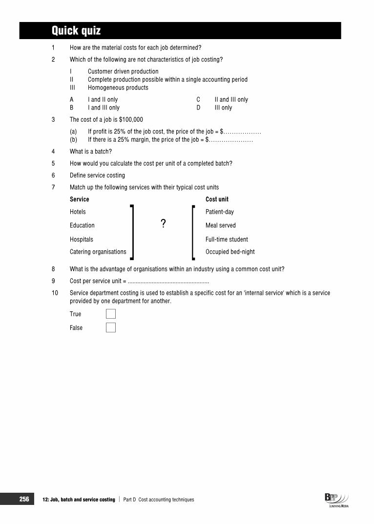
256 12: Job, batch and service costing Part D Cost accounting techniques
Quick quiz 1 How are the material costs for each job determined?
2 Which of the following are not characteristics of job costing?
I Customer driven production II Complete production possible within a single accounting period III Homogeneous products
A I and II only C II and III only B I and III only D III only
3 The cost of a job is $100,000
(a) If profit is 25% of the job cost, the price of the job = $……………… (b) If there is a 25% margin, the price of the job = $…………………
4 What is a batch?
5 How would you calculate the cost per unit of a completed batch?
6 Define service costing
7 Match up the following services with their typical cost units
Service Cost unit
Hotels Patient-day
Education ? Meal served
Hospitals Full-time student
Catering organisations Occupied bed-night
8 What is the advantage of organisations within an industry using a common cost unit?
9 Cost per service unit = ...................................................
10 Service department costing is used to establish a specific cost for an 'internal service' which is a service provided by one department for another.
True
False

Part D Cost accounting techniques 12: Job, batch and service costing 257
Answers to quick quiz 1 From materials requisition notes, or from suppliers' invoices if materials are purchased specifically for a
particular job.
2 D
3 (a) $100,000 + (25% $100,000) = $100,000 + $25,000 = $125,000
(b) Let price of job = x
Profit = 25% x (selling price) If profit = 0.25x x – 0.25x = cost of job 0.75x = $100,000
x = 75.0000,100$
= $133,333
4 A group of similar articles which maintains its identity during one or more stages of production and is treated as a cost unit.
5batch the in units of Number
cost batch Total
6 Cost accounting for services or functions eg canteens, maintenance, personnel (service centres/functions).
7 Service Cost unit
Hotels Patient-day
Education Meal served
Hospitals Full-time student
Catering organisations Occupied bed-night
8 It is easier to make comparisons.
9 Cost per service unit = period the in units service of Number
periodforcostsTotal
10 True
Now try the questions below from the Exam Question Bank
Number Level Marks Time
Q12 MCQ/OTQ n/a n/a

258 12: Job, batch and service costing Part D Cost accounting techniques

259
Budgeting and standard costing
P
A
R
T
E

260

261
Budgeting
IntroductionThis chapter covers a new topic, budgeting. You will meet the topic at all stages of your future examination studies and so it is vital that you get a firm grasp of it now.
The chapter begins by explaining the reasons for operating a budgetary planning and control system (Section 1), explains some of the key terms associated with budgeting and reminds you of the steps in the preparation of a master budget (Section 2).
Topic list Syllabus reference
1 Budgetary planning and control systems E1 (a)
2 The preparation of budgets E1 (b), (c) E2 (a)
3 The sales budget E2 (b)
4 Production and related budgets E2 (b)
5 Fixed and flexible budgets E3 (a)
6 Preparing flexible budgets E3 (a)
7 Flexible budgets and budgetary control E3 (a) E5 (a)
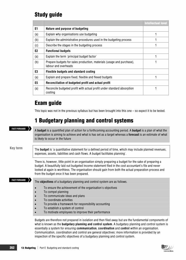
262 13: Budgeting Part E Budgeting and standard costing
Study guide Intellectual level
E1 Nature and purpose of budgeting
(a) Explain why organisations use budgeting 1
(b) Explain the administrative procedures used in the budgeting process 1
(c) Describe the stages in the budgeting process 1
E2 Functional budgets
(a) Explain the term 'principal budget factor' 1
(b) Prepare budgets for sales production, materials (usage and purchase), labour and overheads
1
E3 Flexible budgets and standard costing
(a) Explain and prepare fixed, flexible and flexed budgets 1
E5 Reconciliation of budgeted profit and actual profit
(a) Reconcile budgeted profit with actual profit under standard absorption costing
1
Exam guide This topic was not in the previous syllabus but has been brought into this one – so expect it to be tested.
1 Budgetary planning and control systems
A budget is a quantified plan of action for a forthcoming accounting period. A budget is a plan of what the organisation is aiming to achieve and what is has set as a target whereas a forecast is an estimate of what is likely to occur in the future
The budget is 'a quantitative statement for a defined period of time, which may include planned revenues, expenses, assets, liabilities and cash flows. A budget facilitates planning'.
There is, however, little point in an organisation simply preparing a budget for the sake of preparing a budget. A beautifully laid out budgeted income statement filed in the cost accountant's file and never looked at again is worthless. The organisation should gain from both the actual preparation process and from the budget once it has been prepared.
The objectives of a budgetary planning and control system are as follows.
To ensure the achievement of the organisation's objectives To compel planning To communicate ideas and plans To coordinate activities To provide a framework for responsibility accounting To establish a system of control To motivate employees to improve their performance
Budgets are therefore not prepared in isolation and then filed away but are the fundamental components of what is known as the budgetary planning and control system. A budgetary planning and control system is essentially a system for ensuring communication, coordination and control within an organisation. Communication, coordination and control are general objectives: more information is provided by an inspection of the specific objectives of a budgetary planning and control system.
FAST FORWARD
Key term
FAST FORWARD

Part E Budgeting and standard costing 13: Budgeting 263
Objective Comment
Ensure the achievement of the organisation's objectives
Objectives are set for the organisation as a whole, and for individual departments and operations within the organisation. Quantified expressions of these objectives are then drawn up as targets to be achieved within the timescale of the budget plan.
Compel planning This is probably the most important feature of a budgetary planning and control system. Planning forces management to look ahead, to set out detailed plans for achieving the targets for each department, operation and (ideally) each manager and to anticipate problems. It thus prevents management from relying on ad hoc or uncoordinated planning which may be detrimental to the performance of the organisation. It also helps managers to foresee potential threats or opportunities, so that they may take action now to avoid or minimise the effect of the threats and to take full advantage of the opportunities.
Communicate ideas and plans A formal system is necessary to ensure that each person affected by the plans is aware of what he or she is supposed to be doing. Communication might be one-way, with managers giving orders to subordinates, or there might be a two-way dialogue and exchange of ideas.
Coordinate activities The activities of different departments or sub-units of the organisation need to be coordinated to ensure maximum integration of effort towards common goals. This concept of coordination implies, for example, that the purchasing department should base its budget on production requirements and that the production budget should in turn be based on sales expectations. Although straightforward in concept, coordination is remarkably difficult to achieve, and there is often 'sub-optimality' and conflict between departmental plans in the budget so that the efforts of each department are not fully integrated into a combined plan to achieve the company's best targets.
Provide a framework for responsibility accounting
Budgetary planning and control systems require that managers of budget centres are made responsible for the achievement of budget targets for the operations under their personal control.
Establish a system of control A budget is a yardstick against which actual performance is monitored and assessed. Control over actual performance is provided by the comparisons of actual results against the budget plan. Departures from budget can then be investigated and the reasons for the departures can be divided into controllable and uncontrollablefactors.
Motivate employees to improve their performance
The interest and commitment of employees can be retained via a system of feedback of actual results, which lets them know how well or badly they are performing. The identification of controllable reasons for departures from budget with managers responsible provides an incentive for improving future performance.
Provide a framework for authorisation
Once the budget has been agreed by the directors and senior managers it acts as an authorisation for each budget holder to incur the costs included in the budget centre's budget. As long as the expenditure is included in the formalised budget the budget holder can carry out day to day operations without needing to seek separate authorisation for each item of expenditure.

264 13: Budgeting Part E Budgeting and standard costing
Objective Comment
Provide a basis for performance evaluation
As well as providing a yardstick for control by comparison, the monitoring of actual results compared with the budget can provide a basis for evaluating the performance of the budget holder. As a result of this evaluation the manager might be rewarded, perhaps with a financial bonus or promotion. Alternatively the evaluation process might highlight the need for more investment in staff development and training.
2 The preparation of budgets
One of the optional performance objectives in your PER is ‘Contribute to budget planning and production’. In order to demonstrate competence in this area, you might be expected to prepare detailed budgets based on the best available information. This section and the next few sections in this chapter cover the mechanics of budget preparation which you can put into practice in the workplace. This knowledge will help you towards the fulfilment of the above performance objective.
Having seen why organisations prepare budgets, we will now turn our attention to the mechanics of budget preparation. We will begin by defining and explaining a number of terms.
2.1 Planning
Planning is the establishment of objectives, and the formulation of the policies, strategies and tactics required to achieve them. Planning comprises long-term/strategic planning, and short-term operation planning.
2.1.1 The value of long-term planning
A budgetary planning and control system operating in isolation without any form of long-term planning as a framework is unlikely to produce maximum potential benefits for an organisation.
(a) Without stated long-term objectives, managers do not know what they should be trying to achieve and so there are no criteria against which to assess possible courses of action.
(b) Without long-term planning, budgets may simply be based on a sales forecast. Performance can therefore only be judged in terms of previous years' results, no analysis of the organisation's potential having been carried out.
(c) Many business decisions need to be taken on a long-term basis. For instance, new products cannot simply be introduced when sales of existing products begin to decline. Likewise, capitalequipment cannot necessarily be purchased and installed in the short term if production volumes start to increase.
(d) With long-term planning, limiting factors (other than sales) which might arise can possibly be anticipated, and avoided or overcome.
2.2 The budget period Except for capital expenditure budgets, the budget period is commonly the accounting year (sub-divided into 12 or 13 control periods).
2.3 The budget manual
The budget manual is a collection of instructions governing the responsibilities of persons and the procedures, forms and records relating to the preparation and use of budgetary data.
Key term
Key term

Part E Budgeting and standard costing 13: Budgeting 265
Likely contents of a budget manual
Examples
An explanation of the objectives of the budgetary process
The purpose of budgetary planning and control The objectives of the various stages of the budgetary process The importance of budgets in the long-term planning and administration
of the enterprise
Organisationalstructures
An organisation chart A list of individuals holding budget responsibilities
Principal budgets An outline of each The relationship between them
Administrative details of budget preparation
Membership and terms of reference of the budget committee The sequence in which budgets are to be prepared A timetable
Procedural matters Specimen forms and instructions for their completion Specimen reports Account codes (or a chart of accounts) The name of the budget officer to whom enquiries must be sent
2.4 The responsibility for preparing budgets The initial responsibility for preparing the budget will normally be with the managers (and their subordinates) who will be carrying out the budget, selling goods or services and authorising expenditure. However, the budget is normally set as part of a longer process, involving the authorisation of set targets by senior management and the negotiation process with the budget holders. Depending on the size of the organisation there may be a large number of budget centres and a separate budget holder would be responsible for setting and achieving the budget for the centre.
Examples of the functional budgets that would be prepared and the managers responsible for their preparation are as follows.
(a) The sales manager should draft the sales budget and selling overhead cost centre budgets. (b) The purchasing manager should draft the material purchases budget.(c) The production manager should draft the direct production cost budgets. (d) Various cost centre managers should prepare the individual production, administration and
distribution cost centre budgets for their own cost centre. (e) The cost accountant will analyse the budgeted overheads to determine the overhead absorption
rates for the next budget period.
2.5 Budget committee
The budget committee is the coordinating body in the preparation and administration of budgets.
The coordination and administration of budgets is usually the responsibility of a budget committee (withthe managing director as chairman).
(a) The budget committee is assisted by a budget officer who is usually an accountant. Every part of the organisation should be represented on the committee, so there should be a representative from sales, production, marketing and so on.
(b) Functions of the budget committee
(i) Coordination of the preparation of budgets, which includes the issue of the budget manual (ii) Issuing of timetables for the preparation of functional budgets (iii) Allocation of responsibilities for the preparation of functional budgets
FAST FORWARD

266 13: Budgeting Part E Budgeting and standard costing
(iv) Provision of information to assist in the preparation of budgets (v) Communication of final budgets to the appropriate managers (vi) Comparison of actual results with budget and the investigation of variances (vii) Continuous assessment of the budgeting and planning process, in order to improve the
planning and control function
2.6 Budget preparation Let us now look at the steps involved in the preparation of a budget. The procedures will differ from organisation to organisation, but the step-by-step approach described in this chapter is indicative of the steps followed by many organisations. The preparation of a budget may take weeks or months, and the budget committee may meet several times before the functional budgets are co-ordinated and the master budget is finally agreed.
2.7 The principal budget factor
The principal budget factor should be identified at the beginning of the budgetary process, and the budget for this is prepared before all the others.
After determining the company’s long-term objectives, the first task in the budgetary process is to identify the principal budget factor. This is also known as the key budget factor or limiting budget factor.
The principal budget factor is the factor which limits the activities of an organisation.
Likely principal budget factors
(a) The principal budget factor is usually sales demand: a company is usually restricted from making and selling more of its products because there would be no sales demand for the increased output at a price which would be acceptable/profitable to the company.
(b) Other possible factors
(i) Machine capacity (iii) The availability of key raw materials (ii) Distribution and selling resources (iv) The availability of cash.
Once this factor is defined then the remainder of the budgets can be prepared. For example, if sales are the principal budget factor then the production manager can only prepare his budget after the sales budget is complete.
Management may not know what the limiting budget factor is until a draft budget has been attempted. The first draft budget will therefore usually begin with the preparation of a draft sales budget.
Question Budgets
A company that manufactures and sells a range of products, with sales potential limited by market share, is considering introducing a system of budgeting.
Required
(a) List (in order of preparation) the functional budgets that need to be prepared. (b) State which budgets will comprise the master budget. (c) Consider how the work outlined in (a) and (b) can be coordinated in order for the budgeting
process to be successful.
FAST FORWARD
Key term
Part E Budgeting and standard costing 13: Budgeting 267
Answer(a) The sequence of budget preparation will be roughly as follows.
(i) Sales budget. (The market share limits demand and so sales is the principal budget factor. All other activities will depend upon this forecast.)
(ii) Finished goods inventory budget (in units) (iii) Production budget (in units) (iv) Production resources budgets (materials, machine hours, labour) (v) Overhead budgets for production, administration, selling and distribution, research and
development and so on
Other budgets required will be the capital expenditure budget, the working capital budget (receivables and payables) and, very importantly, the cash budget.
(b) The master budget is the summary of all the functional budgets. It often includes a summary income statement and balance sheet.
(c) Procedures for preparing budgets can be contained in a budget manual which shows which budgets must be prepared when and by whom, what each functional budget should contain and detailed directions on how to prepare budgets including, for example, expected price increases, rates of interest, rates of depreciation and so on.
The formulation of budgets can be coordinated by a budget committee comprising the senior executives of the departments responsible for carrying out the budgets: sales, production, purchasing, personnel and so on.
The budgeting process may also be assisted by the use of a spreadsheet/computer budgeting package.
3 The sales budget We have already established that, for many organisations, the principal budget factor is sales volume. The sales budget is therefore often the primary budget from which the majority of the other budgets are derived.
Before the sales budget can be prepared a sales forecast has to be made. A forecast is an estimate of what is likely to occur in the future. A budget, in contrast, is a plan of what the organisation is aiming to achieve and what it has set as a target.
On the basis of the sales forecast and the production capacity of the organisation, a sales budget will be prepared. This may be subdivided, possible subdivisions being by product, by sales area, by management responsibility and so on.
Once the sales budget has been agreed, related budgets can be prepared.
4 Production and related budgets If the principal budget factor was production capacity then the production budget would be the first to be prepared. To assess whether production is the principal budget factor, the production capacity available must be determined, taking account of a number of factors.
Available labour, including idle time, overtime and standard output rates per hour Availability of raw materials including allowances for losses during production Maximum machine hours available, including expected idle time and expected output rates per machine hour
It is, however, normally sales volume that is the constraint and therefore the production budget is usually prepared after the sales budget and the finished goods inventory budget.

268 13: Budgeting Part E Budgeting and standard costing
The production budget will show the quantities and costs for each product and product group and will tie in with the sales and inventory budgets. This co-ordinating process is likely to show any shortfalls or excesses in capacity at various times over the budget period.
If there is likely to be a shortfall then consideration should be given to how this can be avoided. Possible options include the following.
Overtime working Machine hire Subcontracting New sources of raw materials
A significant shortfall means that production capacity is, in fact, the limiting factor.
If capacity exceeds sales volume for a length of time then consideration should be given to productdiversification, a reduction in selling price (if demand is price elastic) and so on.
Once the production budget has been finalised, the labour, materials and machine budgets can be drawn up. These budgets will be based on budgeted activity levels, planned inventory positions and projected labour and material costs.
4.1 Example: the production budget and direct labour budget Landy manufactures two products, A and B, and is preparing its budget for 20X3. Both products are made by the same grade of labour, grade Q. The company currently holds 800 units of A and 1,200 units of B in inventory, but 250 of these units of B have just been discovered to have deteriorated in quality, and must therefore be scrapped. Budgeted sales of A are 3,000 units and of B 4,000 units, provided that the company maintains finished goods inventories at a level equal to three months' sales.
Grade Q labour was originally expected to produce one unit of A in two hours and one unit of B in three hours, at an hourly rate of $2.50 per hour. In discussions with trade union negotiators, however, it has been agreed that the hourly wage rate should be raised by 50c per hour, provided that the times to produce A and B are reduced by 20%.
Required
Prepare the production budget and direct labour budget for 20X3.
SolutionThe expected time to produce a unit of A will now be 80% of 2 hours = 1.6 hours, and the time for a unit of B will be 2.4 hours. The hourly wage rate will be $3, so that the direct labour cost will be $4.80 for A and $7.20 for B (thus achieving a saving for the company of 20c per unit of A produced and 30c per unit of B).
(a) Production budget Product A Product B
Units Units Units Units Budgeted sales 3,000 4,000 Closing inventories (3
/12 of 3,000) 750 (3/12 of 4,000) 1,000
Opening inventories (minus inventories scrapped) 800 950(Decrease)/increase in inventories (50) 50Production 2,950 4,050
(b) Direct labour budget Grade Q CostHours $
2,950 units of product A 4,720 14,1604,050 units of product B 9,720 29,160Total 14,440 43,320
It is assumed that there will be no idle time among grade Q labour which, if it existed, would have to be paid for at the rate of $3 per hour.

Part E Budgeting and standard costing 13: Budgeting 269
4.2 The standard hour
A standard hour or standard minute is the amount of work achievable at standard efficiency levels in that time period.
This is a useful concept in budgeting for labour requirements. For example, budgeted output of different products or jobs in a period could be converted into standard hours of production, and a labour budget constructed accordingly.
Standard hours are particularly useful when management wants to monitor the production levels of a variety of dissimilar units. For example product A may take five hours to produce and product B, seven hours. If four units of each product are produced, instead of saying that total output is eight units, we could state the production level as (4 5) + (4 7) standard hours = 48 standard hours.
4.3 Example: direct labour budget based on standard hours Truro manufactures a single product, Q, with a single grade of labour. Its sales budget and finished goods inventory budget for period 3 are as follows.
Sales 700 units Opening inventories, finished goods 50 units Closing inventories, finished goods 70 units
The goods are inspected only when production work is completed, and it is budgeted that 10% of finished work will be scrapped.
The standard direct labour hour content of product Q is three hours. The budgeted productivity ratio for direct labour is only 80% (which means that labour is only working at 80% efficiency).
The company employs 18 direct operatives, who are expected to average 144 working hours each in period 3.
Required
(a) Prepare a production budget. (b) Prepare a direct labour budget. (c) Comment on the problem that your direct labour budget reveals, and suggest how this problem
might be overcome.
Solution(a) Production budget
UnitsSales 700Add closing inventory 70
770Less opening inventory 50Production required of 'good' output 720
Wastage rate 10%
Total production required 720 90
*100 = 800 units
(* Note that the required adjustment is 100/90, not 110/100, since the waste is assumed to be 10% of total production, not 10% of good production.)
(b) Now we can prepare the direct labour budget.
Standard hours per unit 3Total standard hours required = 800 units 3 hours 2,400 hours Productivity ratio 80%
Key term

270 13: Budgeting Part E Budgeting and standard costing
Actual hours required 2,400 80
100 = 3,000 hours
(c) If we look at the direct labour budget against the information provided, we can identify the problem.
HoursBudgeted hours available (18 operatives 144 hours) 2,592Actual hours required 3,000Shortfall in labour hours 408
The (draft) budget indicates that there will not be enough direct labour hours to meet the production requirements.
(d) Overcoming insufficient labour hours
(i) Reduce the closing inventory requirement below 70 units. This would reduce the number of production units required.
(ii) Persuade the workforce to do some overtime working.(iii) Perhaps recruit more direct labour if long-term prospects are for higher production
volumes.(iv) Improve the productivity ratio, and so reduce the number of hours required to produce the
output.(v) If possible, reduce the wastage rate below 10%.
4.4 Example: the material purchases budget Tremor manufactures two products, S and T, which use the same raw materials, D and E. One unit of S uses 3 litres of D and 4 kilograms of E. One unit of T uses 5 litres of D and 2 kilograms of E. A litre of D is expected to cost $3 and a kilogram of E $7.
Budgeted sales for 20X2 are 8,000 units of S and 6,000 units of T; finished goods in inventory at 1 January 20X2 are 1,500 units of S and 300 units of T, and the company plans to hold inventories of 600 units of each product at 31 December 20X2.
Inventories of raw material are 6,000 litres of D and 2,800 kilograms of E at 1 January, and the company plans to hold 5,000 litres and 3,500 kilograms respectively at 31 December 20X2.
The warehouse and stores managers have suggested that a provision should be made for damages and deterioration of items held in store, as follows.
Product S : loss of 50 units Material D : loss of 500 litres Product T : loss of 100 units Material E : loss of 200 kilograms
Required
Prepare a material purchases budget for the year 20X2.
SolutionTo calculate material purchase requirements, it is first of all necessary to calculate the budgeted production volumes and material usage requirements.
Product S Product T Units Units Units Units
Sales 8,000 6,000Provision for losses 50 100Closing inventory 600 600Opening inventory 1,500 300(Decrease)/increase in inventory (900) 300Production budget 7,150 6,400

Part E Budgeting and standard costing 13: Budgeting 271
Material D Material E Litres Litres Kg Kg
Usage requirements To produce 7,150 units of S 21,450 28,600 To produce 6,400 units of T 32,000 12,800Usage budget 53,450 41,400Provision for losses 500 200
53,950 41,600Closing inventory 5,000 3,500Opening inventory 6,000 2,800(Decrease)/increase in inventory (1,000) 700Material purchases budget 52,950 42,300
Material D Material E Cost per unit $3 per litre $7 per kg Cost of material purchases $158,850 $296,100Total purchases cost $454,950
Question Material purchases budget
J purchases a basic commodity and then refines it for resale. Budgeted sales of the refined product are as follows.
April May June Sales in kg 9,000 8,000 7,000
The basic raw material costs $3 per kg. Material losses are 10% of finished output. The target month-end raw material inventory level is 5,000 kg plus 25% of the raw material
required for next month's budgeted production. The target month-end inventory level for finished goods is 6,000 kg plus 25% of next month's
budgeted sales.
What are the budgeted raw material purchases for April?
A 8,500 kg C 9,447 kg B 9,350 kg D 9,722 kg
AnswerThe correct answer is C.
March April Maykg kg kg
Required finished inventory: Base inventory 6,000 6,000 6,000 + 25% of next month's sales 2,250 2,000 1,750= Required inventory 8,250 8,000 7,750Sales for month 9,000 8,000
17,000 15,750Less: opening inventory 8,250 8,000Required finished production 8,750 7,750
Wastage rate as % of finished output 10% 10%
Raw material required
8,750 × 90100
7,750 × 90100
= 9,722 kg = 8,611 kg
25% required for closing inventory 2,430.5 kg 2,152.75 kg

272 13: Budgeting Part E Budgeting and standard costing
March April Maykg kg kg
Required material inventory: Base inventory 5,000.00 5,000.00 + 25% of material for next month's production 2,430.50 2,152.75= Required closing material inventory 7,430.50 7,152.75Production requirements 9,722.00
16,874.75Less: opening inventory 7,430.50Required material purchases 9,444.25
4.5 Non-production overheads In the modern business environment, an increasing proportion of overheads are not directly related to the volume of production, such as administration overheads and research and development costs.
4.6 Key decisions in the budgeting process for non-production overheads Deciding which fixed costs are committed (will be incurred no matter what) and which fixed costs will depend on management decisions.
Deciding what factors will influence the level of variable costs. Administration costs for example may be partly governed by the number of orders received.
5 Fixed and flexible budgets
Fixed budgets remain unchanged regardless of the level of activity; flexible budgets are designed to flex with the level of activity.
Flexible budgets are prepared using marginal costing and so mixed costs must be split into their fixed and variable components (possibly using the high/low method).
5.1 Fixed budgets The master budget prepared before the beginning of the budget period is known as the fixed budget. By the term 'fixed', we do not mean that the budget is kept unchanged. Revisions to a fixed master budget will be made if the situation so demands. The term 'fixed' means the following.
(a) The budget is prepared on the basis of an estimated volume of production and an estimated volume of sales, but no plans are made for the event that actual volumes of production and sales may differ from budgeted volumes.
(b) When actual volumes of production and sales during a control period (month or four weeks or quarter) are achieved, a fixed budget is not adjusted (in retrospect) to represent a new target for the new levels of activity.
The major purpose of a fixed budget lies in its use at the planning stage, when it seeks to define the broad objectives of the organisation.
A fixed budget is a budget which is normally set prior to the start of an accounting period, and which is not changed in response to changes in activity or costs/revenues.
Fixed budgets (in terms of a pre-set expenditure limit) are also useful for controlling any fixed cost, and particularly non-production fixed costs such as advertising, because such costs should be unaffected by changes in activity level (within a certain range).
FAST FORWARD
Key term
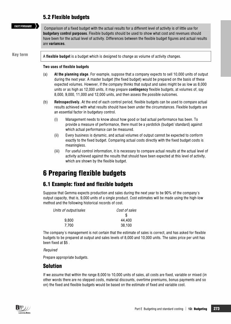
Part E Budgeting and standard costing 13: Budgeting 273
5.2 Flexible budgets
Comparison of a fixed budget with the actual results for a different level of activity is of little use for budgetary control purposes. Flexible budgets should be used to show what cost and revenues should have been for the actual level of activity. Differences between the flexible budget figures and actual results are variances.
A flexible budget is a budget which is designed to change as volume of activity changes.
Two uses of flexible budgets
(a) At the planning stage. For example, suppose that a company expects to sell 10,000 units of output during the next year. A master budget (the fixed budget) would be prepared on the basis of these expected volumes. However, if the company thinks that output and sales might be as low as 8,000 units or as high as 12,000 units, it may prepare contingency flexible budgets, at volumes of, say 8,000, 9,000, 11,000 and 12,000 units, and then assess the possible outcomes.
(b) Retrospectively. At the end of each control period, flexible budgets can be used to compare actual results achieved with what results should have been under the circumstances. Flexible budgets are an essential factor in budgetary control.
(i) Management needs to know about how good or bad actual performance has been. To provide a measure of performance, there must be a yardstick (budget/ standard) against which actual performance can be measured.
(ii) Every business is dynamic, and actual volumes of output cannot be expected to conform exactly to the fixed budget. Comparing actual costs directly with the fixed budget costs is meaningless.
(iii) For useful control information, it is necessary to compare actual results at the actual level of activity achieved against the results that should have been expected at this level of activity, which are shown by the flexible budget.
6 Preparing flexible budgets 6.1 Example: fixed and flexible budgets Suppose that Gemma expects production and sales during the next year to be 90% of the company's output capacity, that is, 9,000 units of a single product. Cost estimates will be made using the high-low method and the following historical records of cost.
Units of output/sales Cost of sales $
9,800 44,400 7,700 38,100
The company's management is not certain that the estimate of sales is correct, and has asked for flexible budgets to be prepared at output and sales levels of 8,000 and 10,000 units. The sales price per unit has been fixed at $5 .
Required
Prepare appropriate budgets.
SolutionIf we assume that within the range 8,000 to 10,000 units of sales, all costs are fixed, variable or mixed (in other words there are no stepped costs, material discounts, overtime premiums, bonus payments and so on) the fixed and flexible budgets would be based on the estimate of fixed and variable cost.
FAST FORWARD
Key term

274 13: Budgeting Part E Budgeting and standard costing
$Total cost of 9,800 units = 44,400 Total cost of 7,700 units = 38,100Variable cost of 2,100 units = 6,300
The variable cost per unit is $3. $ Total cost of 9,800 units = 44,400Variable cost of 9,800 units (9,800 $3) = 29,400Fixed costs (all levels of output and sales) = 15,000
The fixed budgets and flexible budgets can now be prepared as follows.
Flexible budget Fixed budget Flexible budget 8,000 units 9,000 units 10,000 units
$ $ $Sales ( $5) 40,000 45,000 50,000Variable costs ( $3) 24,000 27,000 30,000Contribution 16,000 18,000 20,000Fixed costs 15,000 15,000 15,000Profit 1,000 3,000 5,000
6.2 The need for flexible budgets We have seen that flexible budgets may be prepared in order to plan for variations in the level of activity above or below the level set in the fixed budget. It has been suggested, however, that since many cost items in modern industry are fixed costs, the value of flexible budgets in planning is dwindling.
(a) In many manufacturing industries, plant costs (depreciation, rent and so on) are a very large proportion of total costs, and these tend to be fixed costs.
(b) Wage costs also tend to be fixed, because employees are generally guaranteed a basic wage for a working week of an agreed number of hours.
(c) With the growth of service industries, labour (wages or fixed salaries) and overheads will account for most of the costs of a business, and direct materials will be a relatively small proportion of total costs.
Flexible budgets are nevertheless necessary, and even if they are not used at the planning stage, they must be used for budgetary control variance analysis.
7 Flexible budgets and budgetary control
Budgetary control is based around a system of budget centres. Each centre has its own budget which is the responsibility of the budget holder.
In other words, individual managers are held responsible for investigating differences between budgeted and actual results, and are then expected to take corrective action or amend the plan in the light of actual events.
It is therefore vital to ensure that valid comparisons are being made. Consider the following example.
7.1 Example Penny manufactures a single product, the Darcy. Budgeted results and actual results for May are as follows.
FAST FORWARD

Part E Budgeting and standard costing 13: Budgeting 275
Budget Actual VarianceProduction and sales of 7,500 8,200the Darcy (units)
$ $ $ Sales revenue 75,000 81,000 6,000 (F)Direct materials 22,500 23,500 1,000 (A)Direct labour 15,000 15,500 500 (A)Production overhead 22,500 22,800 300 (A)Administration overhead 10,000 11,000 1,000 (A)
70,000 72,800 2,800 (A)
Profit 5,000 8,200 3,200 (F)
Note. (F) denotes a favourable variance and (A) an unfavourable or adverse variance.
In this example, the variances are meaningless for the purposes of control. All costs were higher than budgeted but the volume of output was also higher; it is to be expected that actual variable costs would be greater those included in the fixed budget. However, it is not possible to tell how much of the increase is due to poor cost control and how much is due to the increase in activity.
Similarly it is not possible to tell how much of the increase in sales revenue is due to the increase in activity. Some of the difference may be due to a difference between budgeted and actual selling price but we are unable to tell from the analysis above.
For control purposes we need to know the answers to questions such as the following.
Were actual costs higher than they should have been to produce and sell 8,200 Darcys? Was actual revenue satisfactory from the sale of 8,200 Darcys?
Instead of comparing actual results with a fixed budget which is based on a different level of activity to that actually achieved, the correct approach to budgetary control is to compare actual results with a budget which has been flexed to the actual activity level achieved.
Suppose that we have the following estimates of the behaviour of Penny's costs.
(a) Direct materials and direct labour are variable costs. (b) Production overhead is a semi-variable cost, the budgeted cost for an activity level of 10,000 units
being $25,000. (c) Administration overhead is a fixed cost. (d) Selling prices are constant at all levels of sales.
SolutionThe budgetary control analysis should therefore be as follows.
Fixed budget Flexible budget Actual results VarianceProduction and sales (units) 7,500 8,200 8,200
$ $ $ $Sales revenue 75,000 82,000 (W1) 81,000 1,000(A)Direct materials 22,500 24,600 (W2) 23,500 1,100 (F)Direct labour 15,000 16,400 (W3) 15,500 900 (F)Production overhead 22,500 23,200 (W4) 22,800 400 (F)Administration overhead 10,000 10,000 (W5) 11,000 1,000 (A)
70,000 74,200 72,800 1,400 (F)
Profit 5,000 7,800 8,200 400 (F)
Workings
(1) Selling price per unit = $75,000 7,500 = $10 per unit Flexible budget sales revenue = $10 8,200 = $82,000
(2) Direct materials cost per unit = $22,500 7,500 = $3 Budget cost allowance = $3 8,200 = $24,600
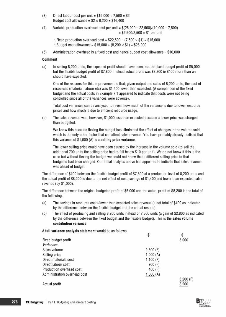
276 13: Budgeting Part E Budgeting and standard costing
(3) Direct labour cost per unit = $15,000 7,500 = $2 Budget cost allowance = $2 8,200 = $16,400
(4) Variable production overhead cost per unit = $(25,000 – 22,500)/(10,000 – 7,500) = $2,500/2,500 = $1 per unit
Fixed production overhead cost = $22,500 – (7,500 $1) = $15,000 Budget cost allowance = $15,000 + (8,200 $1) = $23,200
(5) Administration overhead is a fixed cost and hence budget cost allowance = $10,000
Comment
(a) In selling 8,200 units, the expected profit should have been, not the fixed budget profit of $5,000, but the flexible budget profit of $7,800. Instead actual profit was $8,200 ie $400 more than we should have expected.
One of the reasons for this improvement is that, given output and sales of 8,200 units, the cost of resources (material, labour etc) was $1,400 lower than expected. (A comparison of the fixed budget and the actual costs in Example 7.1 appeared to indicate that costs were not being controlled since all of the variances were adverse).
Total cost variances can be analysed to reveal how much of the variance is due to lower resource prices and how much is due to efficient resource usage.
(b) The sales revenue was, however, $1,000 less than expected because a lower price was charged than budgeted.
We know this because flexing the budget has eliminated the effect of changes in the volume sold, which is the only other factor that can affect sales revenue. You have probably already realised that this variance of $1,000 (A) is a selling price variance.
The lower selling price could have been caused by the increase in the volume sold (to sell the additional 700 units the selling price had to fall below $10 per unit). We do not know if this is the case but without flexing the budget we could not know that a different selling price to that budgeted had been charged. Our initial analysis above had appeared to indicate that sales revenue was ahead of budget.
The difference of $400 between the flexible budget profit of $7,800 at a production level of 8,200 units and the actual profit of $8,200 is due to the net effect of cost savings of $1,400 and lower than expected sales revenue (by $1,000).
The difference between the original budgeted profit of $5,000 and the actual profit of $8,200 is the total of the following.
(a) The savings in resource costs/lower than expected sales revenue (a net total of $400 as indicated by the difference between the flexible budget and the actual results).
(b) The effect of producing and selling 8,200 units instead of 7,500 units (a gain of $2,800 as indicated by the difference between the fixed budget and the flexible budget). This is the sales volume contribution variance.
A full variance analysis statement would be as follows. $ $
Fixed budget profit 5,000VariancesSales volume 2,800 (F)Selling price 1,000 (A)Direct materials cost 1,100 (F)Direct labour cost 900 (F)Production overhead cost 400 (F)Administration overhead cost 1,000 (A)
3,200 (F)Actual profit 8,200

Part E Budgeting and standard costing 13: Budgeting 277
If management believes that any of the variances are large enough to justify it, they will investigate the reasons for their occurrence to see whether any corrective action is necessary.
Question Flexible budget
Flower budgeted to sell 200 units and produced the following budget. $ $
Sales 71,400 Variable costs Labour 31,600 Material 12,600
44,200 Contribution 27,200 Fixed costs 18,900 Profit 8,300
Actual sales turned out to be 230 units, which were sold for $69,000. Actual expenditure on labour was $27,000 and on material $24,000. Fixed costs totalled $10,000.
Required
Prepare a flexible budget that will be useful for management control purposes.
AnswerBudget Bu Budget Flexed budget Actual
200 units per unit 230 units 230 units Variance$ $ $ $ $
Sales 71,400 357 82,110 69,000 13,110 (A)Variable costs Labour 31,600 158 36,340 27,000 9,340 (F) Material 12,600 63 14,490 24,000 9,510 (A)
44,200 221 50,830 51,000Contribution 27,200 136 31,280 18,000 13,280 (A) Fixed costs 18,900 18,900 10,000 8,900 (F)Profit 8,300 12,380 8,000 4,380 (A)
7.2 Flexible budgets, control and computers The production of flexible budget control reports is an area in which computers can provide invaluable assistance to the cost accountant, calculating flexed budget figures using fixed budget and actual results data and hence providing detailed variance analysis. For control information to be of any value it must be produced quickly: speed is one of the many advantages of computers.
7.3 The link between standard costing and budget flexing The calculation of standard cost variances and the use of a flexed budget to control costs and revenues are very similar in concept.
For example, a direct material total variance in a standard costing system is calculated by comparing the material cost that should have been incurred for the output achieved, with the actual cost that was incurred.
Exactly the same process is undertaken when a budget is flexed to provide a basis for comparison with the actual cost: the flexible budget cost allowance for material cost is the same as the cost that should

278 13: Budgeting Part E Budgeting and standard costing
have been incurred for the activity level achieved. In the same way as for standard costing, this is then compared with the actual cost incurred in order to practice control by comparison.
However, there are differences between the two techniques.
(a) Standard costing variance analysis is more detailed. The total material cost variance is analysed further to determine how much of the total variance is caused by a difference in the price paid for materials (the material price variance) and how much is caused by the usage of material being different from the standard (the material usage variance). In flexible budget comparisons only total cost variances are derived.
(b) For a standard costing system to operate it is necessary to determine a standard unit cost for all items of output. All that is required to operate a flexible budgeting system is an understanding of the cost behaviour patterns and a measure of activity to use to flex the budget cost allowance for each cost element.
Make sure you understand the principal budget factor and the difference between fixed and flexiblebudgets.
Chapter Roundup
A budget is a quantified plan of action for a forthcoming accounting period. A budget is a plan of what the organisation is aiming to achieve and what is has set as a target, whereas a forecast is an estimate of what is likely to occur in the future
The objectives of a budgetary planning and control system are as follows.
– To ensure the achievement of the organisation's objectives – To compel planning – To communicate ideas and plans – To coordinate activities – To provide a framework for responsibility accounting – To establish a system of control – To motivate employees to improve their performance
The budget committee is the coordinating body in the preparation and administration of budgets.
The principal budget factor should be identified at the beginning of the budgetary process, and the budget for this is prepared before all the others.
Fixed budgets remain unchanged regardless of the level of activity; flexible budgets are designed to flex with the level of activity.
Flexible budgets are prepared using marginal costing and so mixed costs must be split into their fixed and variable component.
Comparison of a fixed budget with the actual results for a different level of activity is of little use for budgeting control purposes. Flexible budgets should be used to show what cost and revenues should have been for the actual level of activity. Differences between the flexible budget figures and actual results are variances.
Budgetary control is based around a system of budget centres. Each centre has its own budget which is the responsibility of the budget holder.
Exam focus point

Part E Budgeting and standard costing 13: Budgeting 279
Quick Quiz 1 Which of the following is not an objective of a system of budgetary planning and control?
A To establish a system of control B To coordinate activities C To compel planning D To motivate employees to maintain current performance levels
2 Sales is always the principal budget factor and so it is always the first budget to be prepared. True or false?
3 Choose the appropriate words from those highlighted.
A forecast/budget is an estimate/guarantee of what is likely to occur in the future/has happened in the past.
A forecast/budget is a quantified plan/unquantified plan/guess of what the organisation is aiming to achieve/spend.
4 Fill in the blanks.
When preparing a production budget, the quantity to be produced is equal to sales ……………….. opening inventory ……………….. closing inventory.
Answers to Quick Quiz 1 D. The objective is to motivate employees to improve their performance.
2 False. The budget for the principal budget factor must be prepared first, but sales is not always the principal budget factor.
3 A forecast is an estimate of what is likely to occur in the future.
A budget is a quantified plan of what the organisation is aiming to achieve.
4 When preparing a production budget, the quantity to be produced is equal to sales minus opening inventory plus closing inventory.
Now try the questions below from the Exam Question Bank
Number Level Marks Time
Q13 MCQ/OTQ n/a n/a

280 13: Budgeting Part E Budgeting and standard costing

281
Standard costing
IntroductionJust as there are standards for most things in our daily lives (cleanliness in hamburger restaurants, educational achievement of nine year olds, number of trains running on time), there are standards for the costs of products and services. Moreover, just as the standards in our daily lives are not always met, the standards for the costs of products and services are not always met. We will not, however, be considering the standards of cleanliness of hamburger restaurants in this chapter but we will be looking at standards for costs, what they are used for and how they are set.
In the next chapter we will see how standard costing forms the basis of a process called variance analysis, a vital management control tool.
Topic list Syllabus reference
1 What is standard costing? E3 (a)
2 Setting standards E3 (b)
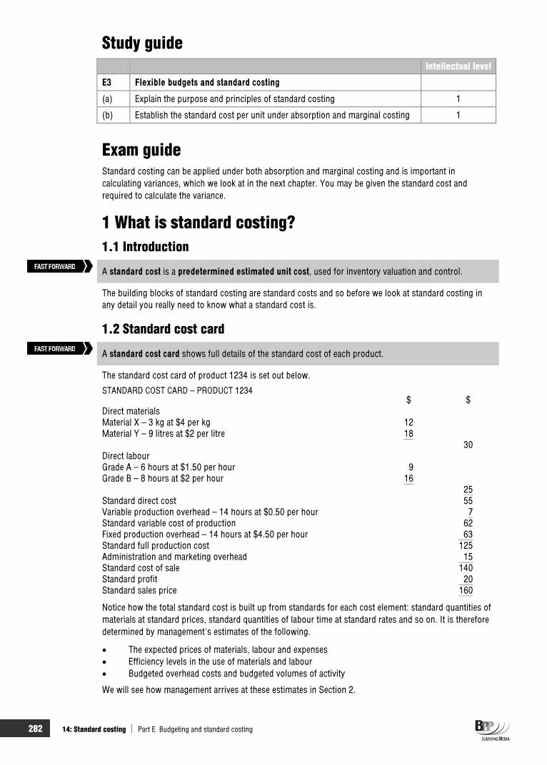
282 14: Standard costing Part E Budgeting and standard costing
Study guide Intellectual level
E3 Flexible budgets and standard costing
(a) Explain the purpose and principles of standard costing 1
(b) Establish the standard cost per unit under absorption and marginal costing 1
Exam guide Standard costing can be applied under both absorption and marginal costing and is important in calculating variances, which we look at in the next chapter. You may be given the standard cost and required to calculate the variance.
1 What is standard costing? 1.1 Introduction
A standard cost is a predetermined estimated unit cost, used for inventory valuation and control.
The building blocks of standard costing are standard costs and so before we look at standard costing in any detail you really need to know what a standard cost is.
1.2 Standard cost card
A standard cost card shows full details of the standard cost of each product.
The standard cost card of product 1234 is set out below.
STANDARD COST CARD – PRODUCT 1234 $ $
Direct materials Material X – 3 kg at $4 per kg 12Material Y – 9 litres at $2 per litre 18
30Direct labourGrade A – 6 hours at $1.50 per hour 9Grade B – 8 hours at $2 per hour 16
25Standard direct cost 55Variable production overhead – 14 hours at $0.50 per hour 7Standard variable cost of production 62Fixed production overhead – 14 hours at $4.50 per hour 63Standard full production cost 125Administration and marketing overhead 15Standard cost of sale 140Standard profit 20Standard sales price 160
Notice how the total standard cost is built up from standards for each cost element: standard quantities of materials at standard prices, standard quantities of labour time at standard rates and so on. It is therefore determined by management's estimates of the following.
The expected prices of materials, labour and expenses Efficiency levels in the use of materials and labour Budgeted overhead costs and budgeted volumes of activity
We will see how management arrives at these estimates in Section 2.
FAST FORWARD
FAST FORWARD

Part E Budgeting and standard costing 14: Standard costing 283
But why should management want to prepare standard costs? Obviously to assist with standard costing, but what is the point of standard costing?
1.3 The uses of standard costing Standard costing has a variety of uses but its two principal ones are as follows.
(a) To value inventories and cost production for cost accounting purposes.(b) To act as a control device by establishing standards (planned costs), highlighting (via variance
analysis which we will cover in the next chapter) activities that are not conforming to plan and thus alerting management to areas which may be out of control and in need of corrective action.
Question Standard cost card
Bloggs makes one product, the joe. Two types of labour are involved in the preparation of a joe, skilled and semi-skilled. Skilled labour is paid $10 per hour and semi-skilled $5 per hour. Twice as many skilled labour hours as semi-skilled labour hours are needed to produce a joe, four semi-skilled labour hours being needed.
A joe is made up of three different direct materials. Seven kilograms of direct material A, four litres of direct material B and three metres of direct material C are needed. Direct material A costs $1 per kilogram, direct material B $2 per litre and direct material C $3 per metre.
Variable production overheads are incurred at Bloggs Co at the rate of $2.50 per direct labour (skilled) hour.
A system of absorption costing is in operation at Bloggs Co. The basis of absorption is direct labour (skilled) hours. For the forthcoming accounting period, budgeted fixed production overheads are $250,000 and budgeted production of the joe is 5,000 units.
Administration, selling and distribution overheads are added to products at the rate of $10 per unit.
A mark-up of 25% is made on the joe.
Required
Using the above information draw up a standard cost card for the joe.
AnswerSTANDARD COST CARD – PRODUCT JOE
Direct materials $ $A – 7 kgs $1 7B – 4 litres $2 8C – 3 m $3 9
24Direct labourSkilled – 8 $10 80Semi-skilled – 4 $5 20
100Standard direct cost 124Variable production overhead – 8 $2.50 20Standard variable cost of production 144Fixed production overhead – 8 $6.25 (W) 50Standard full production cost 194Administration, selling and distribution overhead 10Standard cost of sale 204Standard profit (25% 204) 51Standard sales price 255

284 14: Standard costing Part E Budgeting and standard costing
Working
Overhead absorption rate = 8 000,5
000,250$ = $6.25 per skilled labour hour
Question Marginal costing system
What would a standard cost card for product joe show under a marginal system?
AnswerSTANDARD COST CARD – PRODUCT JOE
$Direct materials 24Direct labour 100Standard direct cost 124Variable production overhead 20Standard variable production cost 144Standard sales price 255Standard contribution 111
Although the use of standard costs to simplify the keeping of cost accounting records should not be overlooked, we will be concentrating on the control and variance analysis aspect of standard costing.
Standard costing is a control technique which compares standard costs and revenues with actual results to obtain variances which are used to improve performance.
Notice that the above definition highlights the control aspects of standard costing.
1.4 Standard costing as a control technique
Differences between actual and standard costs are called variances.
Standard costing therefore involves the following.
The establishment of predetermined estimates of the costs of products or services The collection of actual costs The comparison of the actual costs with the predetermined estimates.
The predetermined costs are known as standard costs and the difference between standard and actual cost is known as a variance. The process by which the total difference between standard and actual results is analysed is known as variance analysis.
Although standard costing can be used in a variety of costing situations (batch and mass production, process manufacture, jobbing manufacture (where there is standardisation of parts) and service industries (if a realistic cost unit can be established)), the greatest benefit from its use can be gained if there is a degree of repetition in the production process. It is therefore most suited to mass production andrepetitive assembly work.
2 Setting standards 2.1 Introduction Standard costs may be used in both absorption costing and in marginal costing systems. We shall, however, confine our description to standard costs in absorption costing systems.
Key term
FAST FORWARD

Part E Budgeting and standard costing 14: Standard costing 285
As we noted earlier, the standard cost of a product (or service) is made up of a number of different standards, one for each cost element, each of which has to be set by management. We have divided this section into two: the first part looks at setting the monetary part of each standard, whereas the second part looks at setting the resources requirement part of each standard.
2.2 Types of performance standard
Performance standards are used to set efficiency targets. There are four types: ideal, attainable, current and basic.
The setting of standards raises the problem of how demanding the standard should be. Should the standard represent a perfect performance or an easily attainable performance? The type of performance standard used can have behavioural implications. There are four types of standard.
Type of standard
Description
Ideal These are based on perfect operating conditions: no wastage, no spoilage, no inefficiencies, no idle time, no breakdowns. Variances from ideal standards are useful for pinpointing areas where a close examination may result in large savings in order to maximise efficiency and minimise waste. However ideal standards are likely to have an unfavourable motivational impact because reported variances will always be adverse. Employees will often feel that the goals are unattainable and not work so hard.
Attainable These are based on the hope that a standard amount of work will be carried out efficiently, machines properly operated or materials properly used. Some allowance is made for wastage and inefficiencies. If well-set they provide a useful psychological incentive by giving employees a realistic, but challenging target of efficiency. The consent and co-operation of employees involved in improving the standard are required.
Current These are based on current working conditions (current wastage, current inefficiencies). The disadvantage of current standards is that they do not attempt to improve on current levels of efficiency.
Basic These are kept unaltered over a long period of time, and may be out of date. They are used to show changes in efficiency or performance over a long period of time. Basic standards are perhaps the least useful and least common type of standard in use.
Ideal standards, attainable standards and current standards each have their supporters and it is by nomeans clear which of them is preferable.
Question Performance standards
Which of the following statements is not true?
A Variances from ideal standards are useful for pinpointing areas where a close examination might result in large cost savings.
B Basic standards may provide an incentive to greater efficiency even though the standard cannot be achieved.
C Ideal standards cannot be achieved and so there will always be adverse variances. If the standards are used for budgeting, an allowance will have to be included for these 'inefficiencies'.
D Current standards or attainable standards are a better basis for budgeting, because they represent the level of productivity which management will wish to plan for.
AnswerThe correct answer is B.
Statement B is describing ideal standards, not basic standards.
FAST FORWARD

286 14: Standard costing Part E Budgeting and standard costing
2.3 Direct material prices Direct material prices will be estimated by the purchasing department from their knowledge of the following.
Purchase contracts already agreed Pricing discussions with regular suppliers The forecast movement of prices in the market The availability of bulk purchase discounts
Price inflation can cause difficulties in setting realistic standard prices. Suppose that a material costs $10 per kilogram at the moment and during the course of the next twelve months it is expected to go up in price by 20% to $12 per kilogram. What standard price should be selected?
The current price of $10 per kilogram The average expected price for the year, say $11 per kilogram
Either would be possible, but neither would be entirely satisfactory.
(a) If the current price were used in the standard, the reported price variance will become adverse as soon as prices go up, which might be very early in the year. If prices go up gradually rather than in one big jump, it would be difficult to select an appropriate time for revising the standard.
(b) If an estimated mid-year price were used, price variances should be favourable in the first half of the year and adverse in the second half of the year, again assuming that prices go up gradually throughout the year. Management could only really check that in any month, the price variance did not become excessively adverse (or favourable) and that the price variance switched from being favourable to adverse around month six or seven and not sooner.
2.4 Direct labour rates Direct labour rates per hour will be set by discussion with the personnel department and by reference to the payroll and to any agreements on pay rises with trade union representatives of the employees.
(a) A separate hourly rate or weekly wage will be set for each different labour grade/type of employee. (b) An average hourly rate will be applied for each grade (even though individual rates of pay may vary
according to age and experience).
Similar problems when dealing with inflation to those described for material prices can be met when setting labour standards.
2.5 Overhead absorption rates When standard costs are fully absorbed costs, the absorption rate of fixed production overheads will be predetermined, usually each year when the budget is prepared, and based in the usual manner on budgeted fixed production overhead expenditure and budgeted production.
For selling and distribution costs, standard costs might be absorbed as a percentage of the standard selling price.
Standard costs under marginal costing will, of course, not include any element of absorbed overheads.
2.6 Standard resource requirements To estimate the materials required to make each product (material usage) and also the labour hours required (labour efficiency), technical specifications must be prepared for each product by production experts (either in the production department or the work study department).
(a) The 'standard product specification' for materials must list the quantities required per unit of each material in the product. These standard input quantities must be made known to the operators in the production department so that control action by management to deal with excess material wastage will be understood by them.

Part E Budgeting and standard costing 14: Standard costing 287
(b) The 'standard operation sheet' for labour will specify the expected hours required by each grade of labour in each department to make one unit of product. These standard times must be carefully set (for example by work study) and must be understood by the labour force. Where necessary, standard procedures or operating methods should be stated.
An exam question may give you actual costs and variances and require you to calculate the standard cost.
Chapter roundup
A standard cost is a predetermined estimated unit cost, used for inventory valuation and control.
A standard cost card shows full details of the standard cost of each product.
Differences between actual and standard cost are called variances.
Performance standards are used to set efficiency targets. There are four types: ideal, attainable, current and basic.
Quick quiz 1 A standard cost is ………………………………………………….. .
2 What are two main uses of standard costing?
3 A control technique which compares standard costs and revenues with actual results to obtain variances which are used to stimulate improved performance is known as:
A Standard costing B Variance analysis C Budgetary control D Budgeting
4 Standard costs may only be used in absorption costing.
True
False
5 Two types of performance standard are
(a) …………………………..
(b) …………………………..
Exam focus point

288 14: Standard costing Part E Budgeting and standard costing
Answers to quick quiz 1 A planned unit cost.
2 (a) To value inventories and cost production for cost accounting purposes. (b) To act as a control device by establishing standards and highlighting activities that are not
conforming to plan and bringing these to the attention of management.
3 A
4 False. They may be used in a marginal costing system as well.
5 (a) Attainable (b) Ideal
Now try the questions below from the Exam Question Bank
Number Level Marks Time
Q14 MCQ/OTQ n/a n/a

289
Basic variance analysis
IntroductionThe actual results achieved by an organisation during a reporting period (week, month, quarter, year) will, more than likely, be different from the expected results (the expected results being the standard costs and revenues which we looked at in the previous chapter). Such differences may occur between individual items, such as the cost of labour and the volume of sales, and between the total expected profit/contribution and the total actual profit/contribution.
Management will have spent considerable time and trouble setting standards. Actual results have differed from the standards. The wise manager will consider the differences that have occurred and use the results of these considerations to assist in attempts to attain the standards. The wise manager will use variance analysis as a method of control.
This chapter examines variance analysis and sets out the method of calculating the variances stated below in the Study Guide. We will then go on to look at the reasons for and significance of cost variances.
Chapter 16 of this Management Accounting Study Text will build on the basics set down in this chapter by introducing sales variances and operatingstatements.
Topic list Syllabus reference
1 Variances E4 (a)
2 Direct material cost variances E4 (a)
3 Direct labour cost variances E4 (a)
4 Variable production overhead variances E4 (a)
5 Fixed production overhead variances E4 (a)
6 The reasons for cost variances E4 (b), (c)
7 The significance of cost variances E4 (d)

290 15: Basic variance analysis Part E Budgeting and standard costing
Study guide Intellectual level
E4 Basic variance analysis under absorption and marginal costing
(a) Calculate the following variances
(i) Materials total, price and usage (ii) Labour total, rate and efficiency (iii) Variable overhead total, expenditure and efficiency (iv) Fixed overhead total, expenditure and, where appropriate, volume
capacity and efficiency
1
(b) Interpret all the variances above 1
(c) Explain possible causes of all the variances above 1
(d) Describe the interrelationships between the variances above 1
Exam guide Variance calculation is a very important part of your Management Accounting studies and it is vital that you are able to calculate all of the different types of variance included in the syllabus.
1 Variances
A variance is the difference between a planned, budgeted, or standard cost and the actual cost incurred. The same comparisons may be made for revenues. The process by which the total difference between standard and actual results is analysed is known as variance analysis.
When actual results are better than expected results, we have a favourable variance (F). If, on the other hand, actual results are worse than expected results, we have an adverse variance (A).
Variances can be divided into three main groups.
Variable cost variances Sales variances Fixed production overhead variances.
In the remainder of this chapter we will consider, in detail, variable cost variances and fixed production overhead variances.
2 Direct material cost variances 2.1 Introduction
The direct material total variance can be subdivided into the direct material price variance and the directmaterial usage variance.
FAST FORWARD
FAST FORWARD

Part E Budgeting and standard costing 15: Basic variance analysis 291
The direct material total variance is the difference between what the output actually cost and what it should have cost, in terms of material.
The direct material price variance. This is the difference between the standard cost and the actual cost for the actual quantity of material used or purchased. In other words, it is the difference between what the material did cost and what it should have cost.
The direct material usage variance. This is the difference between the standard quantity of materials that should have been used for the number of units actually produced, and the actual quantity of materials used, valued at the standard cost per unit of material. In other words, it is the difference between how much material should have been used and how much material was used, valued at standard cost.
2.2 Example: Direct material variances Product X has a standard direct material cost as follows.
10 kilograms of material Y at $10 per kilogram = $100 per unit of X.
During period 4, 1,000 units of X were manufactured, using 11,700 kilograms of material Y which cost $98,600.
Required
Calculate the following variances.
(a) The direct material total variance (b) The direct material price variance (c) The direct material usage variance
Solution(a) The direct material total variance
This is the difference between what 1,000 units should have cost and what they did cost.
$1,000 units should have cost ( $100) 100,000 but did cost 98,600Direct material total variance 1,400 (F)
The variance is favourable because the units cost less than they should have cost.
Now we can break down the direct material total variance into its two constituent parts: the direct material price variance and the direct material usage variance.
(b) The direct material price variance
This is the difference between what 11,700 kgs should have cost and what 11,700 kgs did cost.
$11,700 kgs of Y should have cost ( $10) 117,000 but did cost 98,600Material Y price variance 18,400 (F)
The variance is favourable because the material cost less than it should have.
(c) The direct material usage variance
This is the difference between how many kilograms of Y should have been used to produce 1,000 units of X and how many kilograms were used, valued at the standard cost per kilogram.
Key terms
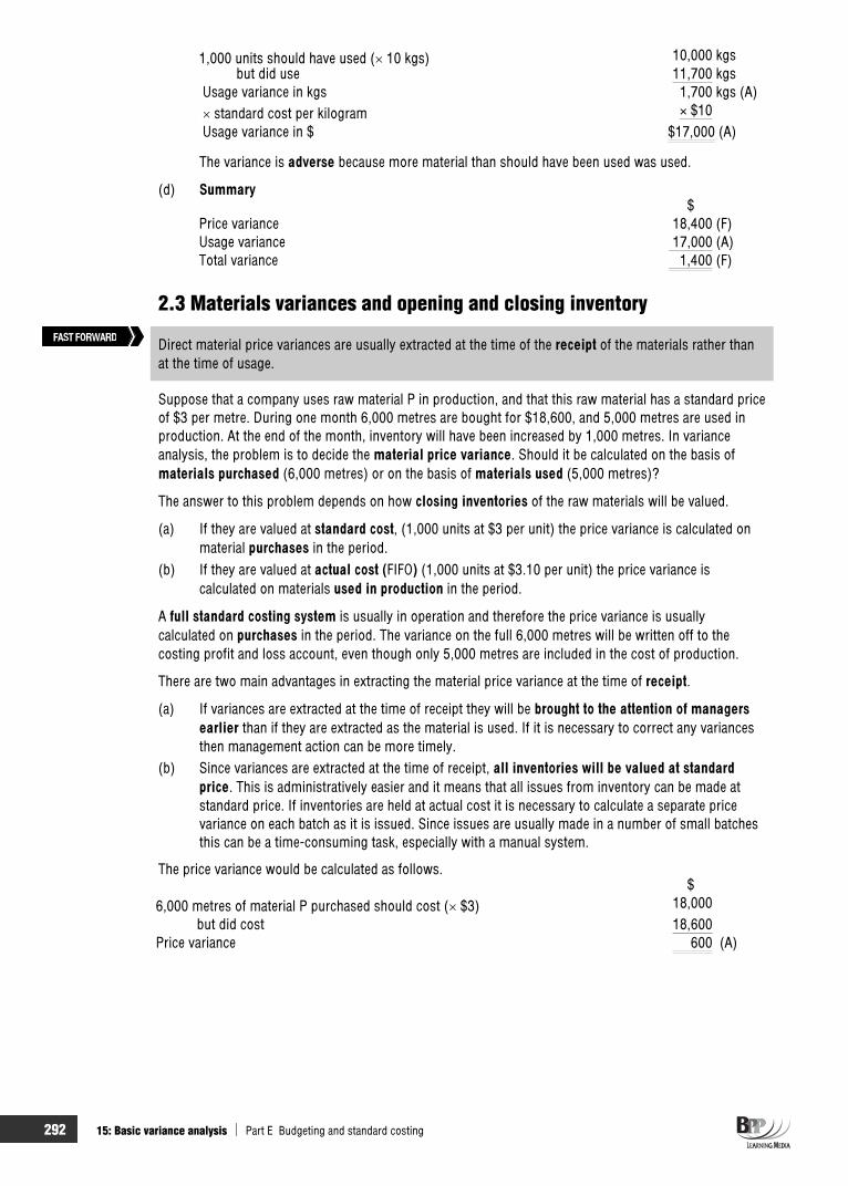
292 15: Basic variance analysis Part E Budgeting and standard costing
1,000 units should have used ( 10 kgs) 10,000 kgs but did use 11,700 kgsUsage variance in kgs 1,700 kgs (A)
standard cost per kilogram × $10Usage variance in $ $17,000 (A)
The variance is adverse because more material than should have been used was used.
(d) Summary$
Price variance 18,400 (F) Usage variance 17,000 (A) Total variance 1,400 (F)
2.3 Materials variances and opening and closing inventory
Direct material price variances are usually extracted at the time of the receipt of the materials rather than at the time of usage.
Suppose that a company uses raw material P in production, and that this raw material has a standard price of $3 per metre. During one month 6,000 metres are bought for $18,600, and 5,000 metres are used in production. At the end of the month, inventory will have been increased by 1,000 metres. In variance analysis, the problem is to decide the material price variance. Should it be calculated on the basis of materials purchased (6,000 metres) or on the basis of materials used (5,000 metres)?
The answer to this problem depends on how closing inventories of the raw materials will be valued.
(a) If they are valued at standard cost, (1,000 units at $3 per unit) the price variance is calculated on material purchases in the period.
(b) If they are valued at actual cost (FIFO) (1,000 units at $3.10 per unit) the price variance is calculated on materials used in production in the period.
A full standard costing system is usually in operation and therefore the price variance is usually calculated on purchases in the period. The variance on the full 6,000 metres will be written off to the costing profit and loss account, even though only 5,000 metres are included in the cost of production.
There are two main advantages in extracting the material price variance at the time of receipt.
(a) If variances are extracted at the time of receipt they will be brought to the attention of managers earlier than if they are extracted as the material is used. If it is necessary to correct any variances then management action can be more timely.
(b) Since variances are extracted at the time of receipt, all inventories will be valued at standard price. This is administratively easier and it means that all issues from inventory can be made at standard price. If inventories are held at actual cost it is necessary to calculate a separate price variance on each batch as it is issued. Since issues are usually made in a number of small batches this can be a time-consuming task, especially with a manual system.
The price variance would be calculated as follows. $
6,000 metres of material P purchased should cost ( $3) 18,000 but did cost 18,600Price variance 600 (A)
FAST FORWARD

Part E Budgeting and standard costing 15: Basic variance analysis 293
3 Direct labour cost variances 3.1 Introduction
The direct labour total variance can be subdivided into the direct labour rate variance and the directlabour efficiency variance.
The direct labour total variance is the difference between what the output should have cost and what it did cost, in terms of labour.
The direct labour rate variance. This is similar to the direct material price variance. It is the differencebetween the standard cost and the actual cost for the actual number of hours paid for.
In other words, it is the difference between what the labour did cost and what it should have cost.
The direct labour efficiency variance is similar to the direct material usage variance. It is the differencebetween the hours that should have been worked for the number of units actually produced, and the actual number of hours worked, valued at the standard rate per hour.
In other words, it is the difference between how many hours should have been worked and how many hours were worked, valued at the standard rate per hour.
The calculation of direct labour variances is very similar to the calculation of direct material variances.
3.2 Example: Direct labour variances The standard direct labour cost of product X is as follows.
2 hours of grade Z labour at $5 per hour = $10 per unit of product X.
During period 4, 1,000 units of product X were made, and the direct labour cost of grade Z labour was $8,900 for 2,300 hours of work.
Required
Calculate the following variances.
(a) The direct labour total variance (b) The direct labour rate variance (c) The direct labour efficiency (productivity) variance
Solution(a) The direct labour total variance
This is the difference between what 1,000 units should have cost and what they did cost.
$1,000 units should have cost ( $10) 10,000
but did cost 8,900Direct labour total variance 1,100 (F)
The variance is favourable because the units cost less than they should have done.
Again we can analyse this total variance into its two constituent parts.
(b) The direct labour rate variance
This is the difference between what 2,300 hours should have cost and what 2,300 hours did cost.
$2,300 hours of work should have cost ( $5 per hr) 11,500 but did cost 8,900Direct labour rate variance 2,600 (F)
Key terms
FAST FORWARD
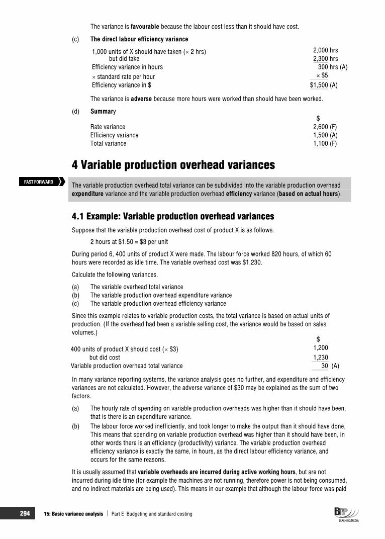
294 15: Basic variance analysis Part E Budgeting and standard costing
The variance is favourable because the labour cost less than it should have cost.
(c) The direct labour efficiency variance
1,000 units of X should have taken ( 2 hrs) 2,000 hrs but did take 2,300 hrsEfficiency variance in hours 300 hrs (A)
standard rate per hour × $5Efficiency variance in $ $1,500 (A)
The variance is adverse because more hours were worked than should have been worked.
(d) Summary$
Rate variance 2,600 (F) Efficiency variance 1,500 (A) Total variance 1,100 (F)
4 Variable production overhead variances The variable production overhead total variance can be subdivided into the variable production overhead expenditure variance and the variable production overhead efficiency variance (based on actual hours).
4.1 Example: Variable production overhead variances Suppose that the variable production overhead cost of product X is as follows.
2 hours at $1.50 = $3 per unit
During period 6, 400 units of product X were made. The labour force worked 820 hours, of which 60 hours were recorded as idle time. The variable overhead cost was $1,230.
Calculate the following variances.
(a) The variable overhead total variance (b) The variable production overhead expenditure variance (c) The variable production overhead efficiency variance
Since this example relates to variable production costs, the total variance is based on actual units of production. (If the overhead had been a variable selling cost, the variance would be based on sales volumes.)
$400 units of product X should cost ( $3) 1,200 but did cost 1,230Variable production overhead total variance 30 (A)
In many variance reporting systems, the variance analysis goes no further, and expenditure and efficiency variances are not calculated. However, the adverse variance of $30 may be explained as the sum of two factors.
(a) The hourly rate of spending on variable production overheads was higher than it should have been, that is there is an expenditure variance.
(b) The labour force worked inefficiently, and took longer to make the output than it should have done. This means that spending on variable production overhead was higher than it should have been, in other words there is an efficiency (productivity) variance. The variable production overhead efficiency variance is exactly the same, in hours, as the direct labour efficiency variance, and occurs for the same reasons.
It is usually assumed that variable overheads are incurred during active working hours, but are not incurred during idle time (for example the machines are not running, therefore power is not being consumed, and no indirect materials are being used). This means in our example that although the labour force was paid
FAST FORWARD

Part E Budgeting and standard costing 15: Basic variance analysis 295
for 820 hours, they were actively working for only 760 of those hours and so variable production overhead spending occurred during 760 hours.
The variable production overhead expenditure variance is the difference between the amount of variable production overhead that should have been incurred in the actual hours actively worked, and the actual amount of variable production overhead incurred.
(a) $760 hours of variable production overhead should cost ( $1.50) 1,140 but did cost 1,230Variable production overhead expenditure variance 90 (A)
The variable production overhead efficiency variance. If you already know the direct labour efficiency variance, the variable production overhead efficiency variance is exactly the same in hours, but priced at the variable production overhead rate per hour.
(b) In our example, the efficiency variance would be as follows.
400 units of product X should take ( 2hrs) 800 hrs but did take (active hours) 760 hrsVariable production overhead efficiency variance in hours 40 hrs (F)
standard rate per hour × $1.50Variable production overhead efficiency variance in $ $60 (F)
(c) Summary$
Variable production overhead expenditure variance 90 (A) Variable production overhead efficiency variance 60 (F)Variable production overhead total variance 30 (A)
5 Fixed production overhead variances
At the ACCA Teachers’ Conference in 2009, the examiner highlighted fixed production overhead variances (particularly the capacity variance) as being an area where students perform poorly. Make sure you study this section carefully and attempt all the questions to ensure you will not be one of these students!
5.1 Introduction
The fixed production overhead total variance can be subdivided into an expenditure variance and a volume variance. The fixed production overhead volume variance can be further subdivided into an efficiency and capacity variance.
You may have noticed that the method of calculating cost variances for variable cost items is essentially the same for labour, materials and variable overheads. Fixed production overhead variances are very different. In an absorption costing system, they are an attempt to explain the under– or over-absorption of fixed production overheads in production costs. We looked at under/over absorption of fixed overheads in Chapter 8.
The fixed production overhead total variance (ie the under– or over-absorbed fixed production overhead) may be broken down into two parts as usual.
An expenditure variance
A volume variance. This in turn may be split into two parts
– A volume efficiency variance – A volume capacity variance
Key term
Key term
FAST FORWARD
Exam focus point
296 15: Basic variance analysis Part E Budgeting and standard costing
You will find it easier to calculate and understand fixed overhead variances, if you keep in mind the whole time that you are trying to 'explain' (put a name and value to) any under– or over-absorbed overhead.
You will need to be able to distinguish between marginal and absorption costing. The variances introduced above and discussed below relate to an absorption costing system. Marginal costing is dealt with in Chapter 16. In the marginal costing system the only fixed overhead variance is an expenditure variance.
5.2 Under/over absorption Remember that the absorption rate is calculated as follows.
Overhead absorption rate =level activity Budgeted
overheadfixedBudgeted
Remember that the budgeted fixed overhead is the planned or expected fixed overhead and the budgeted activity level is the planned or expected activity level.
If either of the following are incorrect, then we will have an under– or over-absorption of overhead.
The numerator (number on top) = Budgeted fixed overhead The denominator (number on bottom) = Budgeted activity level
5.3 The fixed overhead expenditure variance The fixed overhead expenditure variance occurs if the numerator is incorrect. It measures the under– or over-absorbed overhead caused by the actual total overhead being different from the budgeted total overhead.
Therefore, fixed overhead expenditure variance = Budgeted (planned) expenditure – Actual Expenditure.
5.4 The fixed overhead volume variance As we have already stated, the fixed overhead volume variance is made up of the following sub-variances.
Fixed overhead efficiency variance Fixed overhead capacity variance
These variances arise if the denominator (ie the budgeted activity level) is incorrect.
The fixed overhead efficiency and capacity variances measure the under– or over-absorbed overhead caused by the actual activity level being different from the budgeted activity level used in calculating the absorption rate.
There are two reasons why the actual activity level may be different from the budgeted activity level used in calculating the absorption rate.
(a) The workforce may have worked more or less efficiently than the standard set. This deviation is measured by the fixed overhead efficiency variance.
(b) The hours worked by the workforce could have been different to the budgeted hours (regardless of the level of efficiency of the workforce) because of overtime and strikes etc. This deviation from the standard is measured by the fixed overhead capacity variance.
5.5 How to calculate the variances In order to clarify the overhead variances which we have encountered in this section, consider the following definitions which are expressed in terms of how each overhead variance should be calculated.
Exam focus point

Part E Budgeting and standard costing 15: Basic variance analysis 297
Fixed overhead total variance is the difference between fixed overhead incurred and fixed overhead absorbed. In other words, it is the under– or over-absorbed fixed overhead.
Fixed overhead expenditure variance is the difference between the budgeted fixed overhead expenditure and actual fixed overhead expenditure.
Fixed overhead volume variance is the difference between actual and budgeted (planned) volume multiplied by the standard absorption rate per unit.
Fixed overhead volume efficiency variance is the difference between the number of hours that actual production should have taken, and the number of hours actually taken (that is, worked) multiplied by the standard absorption rate per hour.
Fixed overhead volume capacity variance is the difference between budgeted (planned) hours of work and the actual hours worked, multiplied by the standard absorption rate per hour.
You should now be ready to work through an example to demonstrate all of the fixed overhead variances.
5.6 Example: Fixed overhead variances Suppose that a company plans to produce 1,000 units of product E during August 20X3. The expected time to produce a unit of E is five hours, and the budgeted fixed overhead is $20,000. The standard fixed overhead cost per unit of product E will therefore be as follows.
5 hours at $4 per hour = $20 per unit
Actual fixed overhead expenditure in August 20X3 turns out to be $20,450. The labour force manages to produce 1,100 units of product E in 5,400 hours of work.
Task
Calculate the following variances.
(a) The fixed overhead total variance (b) The fixed overhead expenditure variance (c) The fixed overhead volume variance (d) The fixed overhead volume efficiency variance (e) The fixed overhead volume capacity variance
SolutionAll of the variances help to assess the under– or over-absorption of fixed overheads, some in greater detail than others.
(a) Fixed overhead total variance$
Fixed overhead incurred 20,450Fixed overhead absorbed (1,100 units $20 per unit) 22,000Fixed overhead total variance 1,550 (F)(= under-/over-absorbed overhead)
The variance is favourable because more overheads were absorbed than budgeted.
(b) Fixed overhead expenditure variance $
Budgeted fixed overhead expenditure 20,000Actual fixed overhead expenditure 20,450Fixed overhead expenditure variance 450 (A)
The variance is adverse because actual expenditure was greater than budgeted expenditure.
Key terms

298 15: Basic variance analysis Part E Budgeting and standard costing
(c) Fixed overhead volume variance
The production volume achieved was greater than expected. The fixed overhead volume variance measures the difference at the standard rate.
$Actual production at standard rate (1,100 $20 per unit) 22,000
Budgeted production at standard rate (1,000 $20 per unit) 20,000Fixed overhead volume variance 2,000 (F)
The variance is favourable because output was greater than expected.
(i) The labour force may have worked efficiently, and produced output at a faster rate than expected. Since overheads are absorbed at the rate of $20 per unit, more will be absorbed if units are produced more quickly. This efficiency variance is exactly the same in hours as the direct labour efficiency variance, but is valued in $ at the standard absorption rate for fixed overhead.
(ii) The labour force may have worked longer hours than budgeted, and therefore produced more output, so there may be a capacity variance.
(d) Fixed overhead volume efficiency variance
The volume efficiency variance is calculated in the same way as the labour efficiency variance.
1,100 units of product E should take ( 5 hrs) 5,500 hrs but did take 5,400 hrs Fixed overhead volume efficiency variance in hours 100 hrs (F)
standard fixed overhead absorption rate per hour $4 Fixed overhead volume efficiency variance in $ $400 (F)
The labour force has produced 5,500 standard hours of work in 5,400 actual hours and so output is 100 standard hours (or 20 units of product E) higher than budgeted for this reason and the variance is favourable.
(e) Fixed overhead volume capacity variance
The volume capacity variance is the difference between the budgeted hours of work and the actual active hours of work (excluding any idle time).
Budgeted hours of work 5,000 hrsActual hours of work 5,400 hrsFixed overhead volume capacity variance 400 hrs (F)
standard fixed overhead absorption rate per hour $4Fixed overhead volume capacity variance in $ $1,600 (F)
Since the labour force worked 400 hours longer than planned, we should expect output to be 400 standard hours (or 80 units of product E) higher than budgeted and hence the variance is favourable.
The variances may be summarised as follows. $
Expenditure variance 450 (A)Efficiency variance 400 (F)Capacity variance 1,600 (F)Over-absorbed overhead (total variance) $1,550 (F)
Part E Budgeting and standard costing 15: Basic variance analysis 299
In general, a favourable cost variance will arise if actual results are less than expected results. Be aware, however, of the fixed overhead volume variance and the fixed overhead volume capacity variance which give rise to favourable and adverse variances in the following situations.
A favourable fixed overhead volume variance occurs when actual production is greater thanbudgeted (planned) production
An adverse fixed overhead volume variance occurs when actual production is less than budgeted(planned) production
A favourable fixed overhead volume capacity variance occurs when actual hours of work are greater than budgeted (planned) hours of work
An adverse fixed overhead volume capacity variance occurs when actual hours of work are lessthan budgeted (planned) hours of work
Do not worry if you find fixed production overhead variances more difficult to grasp than the other variances we have covered. Most students do. Read over this section again and then try the following practice questions.
Question Capacity variance
A manufacturing company operates a standard absorption costing system. Last month 25,000 production hours were budgeted and the budgeted fixed production overhead cost was $125,000. Last month the actual hours worked were 24,000 and the standard hours for actual production were 27,000.
What was the fixed production overhead capacity variance for last month?
A $5,000 Adverse B $5,000 Favourable C $10,000 Adverse D $10,000 Favourable
AnswerThe correct answer is A.
Standard fixed overhead absorption rate per hour = $125,000/25,000 = $5 per hour
Fixed overhead volume capacity variance Budgeted hours of work 25,000 hrsActual hours of work 24,000 hrsFixed overhead volume capacity variance 1,000 hrs (A)
standard fixed overhead absorption rate per hour $5Fixed overhead volume capacity variance in $ $5,000 (A)
Refer to the exam focus point above for the rules on how to identify an adverse fixed overhead volume capacity variance. Remember that the capacity variance represents part of the over/under absorption of overheads. As the company worked less hours than budgeted (and the standard fixed overhead absorption rate is calculated using budgeted hours) this will result in an under-absorption of overheads.
This question appeared in the December 2008 exam and was answered correctly by less than 40% of students. Almost as many students selected choice B as those who selected the correct choice. Those who selected C or D had obviously calculated the volume variance (which was $10,000 favourable) instead of the capacity variance.
Exam focus point
Exam focus point

300 15: Basic variance analysis Part E Budgeting and standard costing
The following information relates to the questions shown below Barbados has prepared the following standard cost information for one unit of Product Zeta.
Direct materials 4kg @ $10/kg $40.00 Direct labour 2 hours @ $4/hour $8.00 Fixed overheads 3 hours @ $2.50 $7.50
The fixed overheads are based on a budgeted expenditure of $75,000 and budgeted activity of 30,000 hours.
Actual results for the period were recorded as follows.
Production 9,000 units Materials – 33,600 kg $336,000 Labour – 16,500 hours $68,500 Fixed overheads $70,000
Question Material variances
The direct material price and usage variances are:
Material price Material usage $ $ A – 24,000 (F) B – 24,000 (A) C 24,000 (F) – D 24,000 (A) –
AnswerMaterial price variance
$33,600 kg should have cost (× $10/kg) 336,000and did cost 336,000
–Material usage variance
9,000 units should have used ( 4kg) 36,000 kgbut did use 33,600 kg
2,400 kg (F) standard cost per kg × $10
24,000 (F)The correct answer is therefore A.
Question Labour variances
The direct labour rate and efficiency variances are: Labour rate Labour efficiency
$ $ A 6,000 (F) 2,500 (A) B 6,000 (A) 2,500 (F) C 2,500 (A) 6,000 (F) D 2,500 (F) 6,000 (A)

Part E Budgeting and standard costing 15: Basic variance analysis 301
AnswerDirect labour rate variance
$ 16,500 hrs should have cost ( $4) 66,000 but did cost 68,500
2,500 (A)Direct labour efficiency variance
9,000 units should have taken ( 2 hrs) 18,000 hrs but did take 16,500 hrs
1,500 (F) standard rate per hour ( $4) × $4
6,000 (F)
The correct answer is therefore C.
Question Overhead variances
The total fixed production overhead variance is:
A $5,000 (A) B $5,000 (F) C $2,500 (A) D $2,500 (F)
Answer$
Fixed production overhead absorbed ($7.50 9,000) 67,500Fixed production overhead incurred 70,000
2,500 (A)
The correct answer is therefore C.
6 The reasons for cost variances
One of the optional performance objectives in your PER is being able to monitor and control budgets. One of the skills you need in order to fulfil this objective is to compare actual figures with budget and identify and explain any differences. This section can be used to help you to develop that skill in the workplace.
There are many possible reasons for cost variances arising, as you will see from the following list of possible causes.
This is not an exhaustive list and in an examination question you should review the information given and use your imagination and common sense in analysing possible reasons for variances.
At the ACCA Teachers’ Conference in 2009, the examiner pointed out that students perform poorly in written questions on variances. Make sure you are not one of them by reading sections 6 and 7 carefully.
Exam focus point

302 15: Basic variance analysis Part E Budgeting and standard costing
Variance Favourable Adverse
(a) Material price Unforeseen discounts received More care taken in purchasing Change in material standard
Price increase Careless purchasing Change in material standard
(b) Material usage Material used of higher quality than standardMore effective use made of material Errors in allocating material to jobs
Defective material Excessive waste TheftStricter quality control Errors in allocating material to jobs
(c) Labour rate Use of apprentices or other workers at a rate of pay lower than standard
Wage rate increase Use of higher grade labour
(d) Idle time The idle time variance is always adverse Machine breakdown Non-availability of material Illness or injury to worker
(e) Labour efficiency Output produced more quickly than expected because of work motivation, better quality of equipment or materials, or better methods. Errors in allocating time to jobs
Lost time in excess of standard allowedOutput lower than standard set because of deliberate restriction, lack of training, or sub-standard material used Errors in allocating time to jobs
(f) Overhead expenditure
Savings in costs incurred More economical use of services
Increase in cost of services used Excessive use of services Change in type of services used
(g) Overhead volume efficiency
Labour force working more efficiently (favourable labour efficiency variance)
Labour force working less efficiently (adverse labour efficiency variance)
(h) Overhead volume capacity
Labour force working overtime Machine breakdown, strikes, labour shortages
7 The significance of cost variances 7.1 Introduction
Materiality, controllability, the type of standard being used, the interdependence of variances and the cost of an investigation should be taken into account when deciding whether to investigate reported variances.
Once variances have been calculated, management have to decide whether or not to investigate their causes. It would be extremely time consuming and expensive to investigate every variance therefore managers have to decide which variances are worthy of investigation.
There are a number of factors which can be taken into account when deciding whether or not a variance should be investigated.
(a) Materiality. A standard cost is really only an average expected cost and is not a rigid specification. Small variations either side of this average are therefore bound to occur. The problem is to decide whether a variation from standard should be considered significant and worthy of investigation. Tolerance limits can be set and only variances which exceed such limits would require investigating.
(b) Controllability. Some types of variance may not be controllable even once their cause is discovered. For example, if there is a general worldwide increase in the price of a raw material there is nothing that can be done internally to control the effect of this. If a central decision is made to award all employees a 10% increase in salary, staff costs in division A will increase by this amount
FAST FORWARD

Part E Budgeting and standard costing 15: Basic variance analysis 303
and the variance is not controllable by division A's manager. Uncontrollable variances call for a change in the plan, not an investigation into the past.
(c) The type of standard being used.
(i) The efficiency variance reported in any control period, whether for materials or labour, will depend on the efficiency level set. If, for example, an ideal standard is used, variances will always be adverse.
(ii) A similar problem arises if average price levels are used as standards. If inflation exists, favourable price variances are likely to be reported at the beginning of a period, to be offset by adverse price variances later in the period as inflation pushes prices up.
(d) Interdependence between variances . Quite possibly, individual variances should not be looked at in isolation. One variance might be inter-related with another, and much of it might have occurred only because the other, inter-related, variance occurred too. We will investigate this issue further in a moment.
(e) Costs of investigation. The costs of an investigation should be weighed against the benefits of correcting the cause of a variance.
7.2 Interdependence between variancesWhen two variances are interdependent (interrelated) one will usually be adverse and the other one favourable.
7.3 Interdependence – materials price and usage variancesIt may be decided to purchase cheaper materials for a job in order to obtain a favourable price variance.This may lead to higher materials wastage than expected and therefore, adverse usage variances occur. If the cheaper materials are more difficult to handle, there might be some adverse labour efficiency variance too.
If a decision is made to purchase more expensive materials, which perhaps have a longer service life, the price variance will be adverse but the usage variance might be favourable.
7.4 Interdependence – labour rate and efficiency variancesIf employees in a workforce are paid higher rates for experience and skill, using a highly skilled team should incur an adverse rate variance at the same time as a favourable efficiency variance. In contrast, a favourable rate variance might indicate a high proportion of inexperienced workers in the workforce, which could result in an adverse labour efficiency variance and possibly an adverse materials usage variance (due to high rates of rejects).

304 15: Basic variance analysis Part E Budgeting and standard costing
Chapter roundup
A variance is the difference between a planned, budgeted, or standard cost and the actual cost incurred. The same comparisons can be made for revenues. The process by which the total difference between standard and actual results is analysed is known as the variance analysis.
The direct material total variance can be subdivided into the direct material price variance and the directmaterial usage variance.
Direct material price variances are usually extracted at the time of receipt of the materials, rather than at the time of usage.
The direct labour total variance can be subdivided into the direct labour rate variance and the directlabour efficiency variance.
If idle time arises, it is usual to calculate a separate idle time variance, and to base the calculation of the efficiency variance on active hours ( when labour actually worked) only. It is always an adverse variance.
The variable production overhead total variance can be subdivided into the variable production overhead expenditure variance and the variable production overhead efficiency variance (based on active hours).
The fixed production overhead total variance can be subdivided into an expenditure variance and a volume variance. The fixed production overhead volume variance can be further subdivided into an efficiency and a capacity variance.
Materiality, controllability, the type of standard being used, the interdependence of variances and the cost of an investigation should be taken into account when deciding whether to investigate reported variances.
Quick quiz 1 Subdivide the following variances.
(a) Direct materials cost variance
(b) Direct labour cost variance
(c) Variable production overhead variance
2 What are the two main advantages in calculating the material price variance at the time of receipt of materials?
3 Idle time variances are always adverse.
True
False
4 Adverse material usage variances might occur for the following reasons.
I Defective material II Excessive waste III Theft IV Unforeseen discounts received
A I B I and II C I, II and III D I, II, III and IV
5 List the factors which should be taken into account when deciding whether or not a variance should be investigated.

Part E Budgeting and standard costing 15: Basic variance analysis 305
Answers to quick quiz
Price 1 (a) Usage
Rate (b) Efficiency
Expenditure (c) Efficiency
2 (a) The earlier variances are extracted, the sooner they will be brought to the attention of managers. (b) All inventories will be valued at standard price which requires less administration effort.
3 True
4 C
5 Materiality Interdependence between variances Controllability Costs of investigation Type of standard being used
Now try the questions below from the Exam Question Bank
Number Level Marks Time
Q15 MCQ/OTQ n/a n/a

306 15: Basic variance analysis Part E Budgeting and standard costing

307
Furthervariance analysis
IntroductionThe objective of cost variance analysis, which we looked at in the previous chapter, is to assist management in the control of costs. Costs are, however, only one factor which contribute to the achievement of planned profit. Salesare another important factor and sales variances can be calculated to aid management's control of their business. We will therefore begin this chapter by examining sales variances.
Having discussed the variances you need to know about, we will be looking in Section 2 at the ways in which variances should be presented to management to aid their control of the organisation.
We then consider in Section 3 how marginal cost variances differ from absorption cost variances and how marginal costing information should be presented.
Finally we will consider how actual data can be derived from standard cost details and variances.
Topic list Syllabus reference
1 Sales variances E4 (a)
2 Operating statements E5 (a), (b)
3 Variances in a standard marginal costing system E4 (b)
4 Deriving actual data from standard cost details and variances E4 (b)

308 16: Further variance analysis Part E Budgeting and standard costing
Study guide Intellectual level
E4 Basic variance analysis under absorption and marginal costing
(a) Calculate interpret and explain sales price and volume variance 1
(b) Calculate actual or standard figures where the following variances are given:
(i) Sales price and volume (ii) Materials total, price and usage (iii) Labour total, rate and efficiency (iv) Variable overhead total, expenditure and efficiency (v) Fixed overhead total, expenditure and, where appropriate, volume,
capacity and efficiency
1
E5 Reconciliation of budgeted profit and actual profit
(a) Reconcile budgeted profit with actual profit under standard absorption costing
1
(b) Reconcile budgeted profit or contribution with actual profit or contribution under standard marginal costing
1
Exam guide Variance analysis is traditionally a very popular exam topic. Make sure that you are able to prepare operating statements and explain why calculated variances have occurred. You will not be expected to prepare a whole operating statement in the exam, but you may be tested on your understanding of these statements.
1 Sales variances1.1 Selling price variance
The selling price variance is a measure of the effect on expected profit of a different selling price to standard selling price. It is calculated as the difference between what the sales revenue should have been for the actual quantity sold, and what it was.
1.2 Example: Selling price variance Suppose that the standard selling price of product X is $15. Actual sales in 20X3 were 2,000 units at $15.30 per unit. The selling price variance is calculated as follows.
$Sales revenue from 2,000 units should have been ( $15) 30,000
but was ( $15.30) 30,600Selling price variance 600 (F)
The variance calculated is favourable because the price was higher than expected.
1.3 Sales volume profit variance
The sales volume profit variance is the difference between the actual units sold and the budgeted (planned) quantity, valued at the standard profit per unit. In other words, it measures the increase or decrease in standard profit as a result of the sales volume being higher or lower than budgeted (planned).
FAST FORWARD
FAST FORWARD

Part E Budgeting and standard costing 16: Further variance analysis 309
1.4 Example: Sales volume profit variance Suppose that a company budgets to sell 8,000 units of product J for $12 per unit. The standard full cost per unit is $7. Actual sales were 7,700 units, at $12.50 per unit.
The sales volume profit variance is calculated as follows.
Budgeted sales volume 8,000 unitsActual sales volume 7,700 unitsSales volume variance in units 300 units (A)
standard profit per unit ($(12–7)) × $5Sales volume variance $1,500 (A)
The variance calculated above is adverse because actual sales were less than budgeted (planned).
Question Selling price variance
Jasper Co has the following budget and actual figures for 20X4. Budget Actual
Sales units 600 620 Selling price per unit $30 $29
Standard full cost of production = $28 per unit.
Required
Calculate the selling price variance and the sales volume profit variance.
AnswerSales revenue for 620 units should have been ( $30) 18,600
but was ( $29) 17,980Selling price variance 620 (A)
Budgeted sales volume 600 unitsActual sales volume 620 unitsSales volume variance in units 20 units (F)
standard profit per unit ($(30 – 28)) × $2 Sales volume profit variance $40 (F)
1.5 The significance of sales variances The possible interdependence between sales price and sales volume variances should be obvious to you. A reduction in the sales price might stimulate bigger sales demand, so that an adverse sales price variance might be counterbalanced by a favourable sales volume variance. Similarly, a price rise would give a favourable price variance, but possibly at the cost of a fall in demand and an adverse sales volume variance.
It is therefore important in analysing an unfavourable sales variance that the overall consequence should be considered, that is, has there been a counterbalancing favourable variance as a direct result of the unfavourable one?

310 16: Further variance analysis Part E Budgeting and standard costing
2 Operating statements 2.1 Introduction
Operating statements show how the combination of variances reconcile budgeted profit and actual profit.
So far, we have considered how variances are calculated without considering how they combine to reconcile the difference between budgeted profit and actual profit during a period. This reconciliation is usually presented as a report to senior management at the end of each control period. The report is called an operating statement or statement of variances.
An operating statement is a regular report for management of actual costs and revenues, usually showing variances from budget.
An extensive example will now be introduced, both to revise the variance calculations already described, and also to show how to combine them into an operating statement.
2.2 Example: Variances and operating statements Sydney manufactures one product, and the entire product is sold as soon as it is produced. There are no opening or closing inventories and work in progress is negligible. The company operates a standard costing system and analysis of variances is made every month. The standard cost card for the product, a boomerang, is as follows.
STANDARD COST CARD – BOOMERANG $
Direct materials 0.5 kilos at $4 per kilo 2.00Direct wages 2 hours at $2.00 per hour 4.00Variable overheads 2 hours at $0.30 per hour 0.60Fixed overhead 2 hours at $3.70 per hour 7.40Standard cost 14.00 Standard profit 6.00Standing selling price 20.00
Selling and administration expenses are not included in the standard cost, and are deducted from profit as a period charge.
Budgeted (planned) output for the month of June 20X7 was 5,100 units. Actual results for June 20X7 were as follows.
Production of 4,850 units was sold for $95,600. Materials consumed in production amounted to 2,300 kgs at a total cost of $9,800. Labour hours paid for amounted to 8,500 hours at a cost of $16,800. Actual operating hours amounted to 8,000 hours. Variable overheads amounted to $2,600. Fixed overheads amounted to $42,300. Selling and administration expenses amounted to $18,000.
Required
Calculate all variances and prepare an operating statement for the month ended 30 June 20X7.
Key term
FAST FORWARD

Part E Budgeting and standard costing 16: Further variance analysis 311
Solution(a) $
2,300 kg of material should cost ( $4) 9,200 but did cost 9,800Material price variance 600 (A)
(b) 4,850 boomerangs should use ( 0.5 kgs) 2,425 kg but did use 2,300 kgMaterial usage variance in kgs 125 kg (F)
standard cost per kg × $4Material usage variance in $ $ 500 (F)
(c) $8,500 hours of labour should cost ( $2) 17,000 but did cost 16,800Labour rate variance 200 (F)
(d) 4,850 boomerangs should take ( 2 hrs) 9,700 hrs but did take (active hours) 8,000 hrsLabour efficiency variance in hours 1,700 hrs (F)
standard cost per hour × $2Labour efficiency variance in $ $3,400 (F)
(e) Idle time variance 500 hours (A) $2 $1,000 (A)
(f) $8,000 hours incurring variable o/hd expenditure should cost ( $0.30) 2,400 but did cost 2,600Variable overhead expenditure variance 200 (A)
(g) Variable overhead efficiency variance in hours is the same as the labour efficiency variance: 1,700 hours (F) $0.30 per hour $ 510 (F)
(h) $Budgeted fixed overhead (5,100 units 2 hrs $3.70) 37,740Actual fixed overhead 42,300Fixed overhead expenditure variance 4,560 (A)
(i) $4,850 boomerangs should take ( 2 hrs) 9,700 hrs but did take (active hours) 8,000 hrs Fixed overhead volume efficiency variance in hrs 1,700 hrs (F)
standard fixed overhead absorption rate per hour $3.70Fixed overhead volume efficiency variance in $ 6,290 (F)
(j) $Budgeted hours of work (5,100 2 hrs) 10,200 hrsActual hours of work 8,000 hrs Fixed overhead volume capacity variance in hrs 2,200 hrs (A)
standard fixed overhead absorption rate per hour $3.70Fixed overhead volume capacity variance in $ 8,140 (A)

312 16: Further variance analysis Part E Budgeting and standard costing
(k) $Revenue from 4,850 boomerangs should be ( $20) 97,000 but was 95,600Selling price variance 1,400 (A)
(l) Budgeted sales volume 5,100 units Actual sales volume 4,850 unitsSales volume profit variance in units 250 units
standard profit per unit × $6 (A) Sales volume profit variance in $ $1,500 (A)
There are several ways in which an operating statement may be presented. Perhaps the most common format is one which reconciles budgeted profit to actual profit. In this example, sales and administration costs will be introduced at the end of the statement, so that we shall begin with 'budgeted profit before sales and administration costs'.
Sales variances are reported first, and the total of the budgeted profit and the two sales variances results in a figure for 'actual sales minus the standard cost of sales'. The cost variances are then reported, and an actual profit (before sales and administration costs) calculated. Sales and administration costs are then deducted to reach the actual profit for June 20X7.
SYDNEY – OPERATING STATEMENT JUNE 20X7 $ $
Budgeted (planned) profit before sales and administration costs 30,600Sales variances: price 1,400 (A) volume 1,500 (A)
2,900 (A)Actual sales minus the standard cost of sales 27,700
(F) (A)Cost variances $ $Material price 600Material usage 500 Labour rate 200 Labour efficiency 3,400 Labour idle time 1,000Variable overhead expenditure 200Variable overhead efficiency 510 Fixed overhead expenditure 4,560Fixed overhead volume efficiency 6,290 Fixed overhead volume capacity 8,140
10,900 14,500 3,600 (A)Actual profit before sales and administration costs 24,100Sales and administration costs 18,000Actual profit, June 20X7 6,100
Check $ $Sales 95,600Materials 9,800Labour 16,800Variable overhead 2,600Fixed overhead 42,300Sales and administration 18,000
89,500Actual profit 6,100

Part E Budgeting and standard costing 16: Further variance analysis 313
3 Variances in a standard marginal costing system
At the ACCA Teachers’ Conference in 2009, the examiner highlighted this area as being one where students perform poorly in the exam. You will note that there are two past exam questions in this section – less than one third of students answered these questions correctly. Make sure you study this section carefully to ensure you understand the techniques before attempting the questions.
3.1 Introduction
There are two main differences between the variances calculated in an absorption costing system and the variances calculated in a marginal costing system.
In the marginal costing system the only fixed overhead variance is an expenditure variance. The sales volume variance is valued at standard contribution margin, not standard profit margin.
In all of the examples we have worked through so far, a system of standard absorption costing has been in operation. If an organisation uses standard marginal costing instead of standard absorption costing, there will be two differences in the way the variances are calculated.
(a) In marginal costing, fixed costs are not absorbed into product costs and so there are no fixed cost variances to explain any under or over absorption of overheads. There will, therefore, be no fixedoverhead volume variance. There will be a fixed overhead expenditure variance which is calculated in exactly the same way as for absorption costing systems.
(b) The sales volume variance will be valued at standard contribution margin (sales price per unit minus variable costs of sale per unit), not standard profit margin.
3.2 Preparing a marginal costing operating statement Returning once again to the example of Sydney, the variances in a system of standard marginal costing would be as follows.
(a) There is no fixed overhead volume variance (and therefore no fixed overhead volume efficiency and volume capacity variances).
(b) The standard contribution per unit of boomerang is $(20 – 6.60) = $13.40, therefore the salesvolume contribution variance of 250 units (A) is valued at ( $13.40) = $3,350 (A).
The other variances are unchanged. However, this operating statement differs from an absorption costing operating statement in the following ways.
(a) It begins with the budgeted contribution ($30,600 + budgeted fixed production costs $37,740 = $68,340).
(b) The subtotal before the analysis of cost variances is actual sales ($95,600) less the standard variable cost of sales ($4,850 $6.60) = $63,590.
(c) Actual contribution is highlighted in the statement. (d) Budgeted (planned) fixed production overhead is adjusted by the fixed overhead expenditure
variance to show the actual fixed production overhead expenditure.
Therefore a marginal costing operating statement might look like this.
FAST FORWARD
Exam focus point

314 16: Further variance analysis Part E Budgeting and standard costing
SYDNEY – OPERATING STATEMENT JUNE 20X7 $ $ $
Budgeted (planned) contribution 68,340Sales variances: volume 3,350 (A) price 1,400 (A)
4,750 (A)Actual sales minus the standard variable cost of sales 63,590
(F) (A)Variable cost variances Material price 600Material usage 500 Labour rate 200 Labour efficiency 3,400 Labour idle time 1,000Variable overhead expenditure 200Variable overhead efficiency 510
4,610 1,800 2,810 (F)
Actual contribution 66,400Budgeted (planned) fixed production overhead 37,740Expenditure variance 4,560 (A)Actual fixed production overhead 42,300Actual profit before sales and administration costs 24,100Sales and administration costs 18,000Actual profit 6,100
Notice that the actual profit is the same as the profit calculated by standard absorption costing because there were no changes in inventory levels. Absorption costing and marginal costing do not always produce an identical profit figure.
Question Variances
Piglet, a manufacturing firm, operates a standard marginal costing system. It makes a single product, PIG, using a single raw material LET.
Standard costs relating to PIG have been calculated as follows.
Standard cost schedule – PIG Per unit$
Direct material, LET, 100 kg at $5 per kg 500Direct labour, 10 hours at $8 per hour 80Variable production overhead, 10 hours at $2 per hour 20
600The standard selling price of a PIG is $900 and Piglet Co produce 1,020 units a month.
During December 20X0, 1,000 units of PIG were produced. Relevant details of this production are as follows.
Direct material LET
90,000 kgs costing $720,000 were bought and used.
Direct labour
8,200 hours were worked during the month and total wages were $63,000.
Variable production overhead
The actual cost for the month was $25,000.
Inventories of the direct material LET are valued at the standard price of $5 per kg.
Each PIG was sold for $975.

Part E Budgeting and standard costing 16: Further variance analysis 315
Required
Calculate the following for the month of December 20X0.
(a) Variable production cost variance (b) Direct labour cost variance, analysed into rate and efficiency variances (c) Direct material cost variance, analysed into price and usage variances (d) Variable production overhead variance, analysed into expenditure and efficiency variances (e) Selling price variance (f) Sales volume contribution variance
Answer(a) This is simply a 'total' variance.
$1,000 units should have cost ( $600) 600,000 but did cost (see working) 808,000Variable production cost variance 208,000 (A)
(b) Direct labour cost variances$
8,200 hours should cost ( $8) 65,600 but did cost 63,000Direct labour rate variance 2,600 (F)
1,000 units should take ( 10 hours) 10,000 hrs but did take 8,200 hrsDirect labour efficiency variance in hrs 1,800 hrs (F)
standard rate per hour × $8Direct labour efficiency variance in $ $14,400 (F)
Summary $Rate 2,600 (F)Efficiency 14,400 (F)Total 17,000 (F)
(c) Direct material cost variances$
90,000 kg should cost ( $5) 450,000 but did cost 720,000Direct material price variance 270,000 (A)
1,000 units should use ( 100 kg) 100,000 kg but did use 90,000 kgDirect material usage variance in kgs 10,000 kg (F)
standard cost per kg × $5Direct material usage variance in $ $50,000 (F)
Summary $Price 270,000 (A)Usage 50,000 (F)Total 220,000 (A)
(d) Variable production overhead variances$
8,200 hours incurring o/hd should cost ( $2) 16,400 but did cost 25,000Variable production overhead expenditure variance 8,600 (A)

316 16: Further variance analysis Part E Budgeting and standard costing
Efficiency variance in hrs (from (b)) 1,800 hrs (F) standard rate per hour × $2
Variable production overhead efficiency variance $3,600 (F)
Summary $
Expenditure 8,600 (A) Efficiency 3,600 (F) Total 5,000 (A)
(e) Selling price variance$
Revenue from 1,000 units should have been ( $900) 900,000
but was ( $975) 975,000Selling price variance 75,000 (F)
(f) Sales volume contribution variance
Budgeted sales 1,020 unitsActual sales 1,000 unitsSales volume variance in units 20 units (A)
standard contribution margin ($(900 – 600)) × $300Sales volume contribution variance in $ $6,000 (A)
Workings $
Direct material 720,000Total wages 63,000Variable production overhead 25,000
808,000
The question above is much longer than what will appear in your exam, but any one of these variances, individually, may be the subject of a 2-mark question.
Question Reconciling contributions
A company uses standard marginal costing. Last month the standard contribution on actual sales was $10,000 and the following variances arose.
$Total variable costs variance 2,000 (A) Sales price variance 500 (F) Sales volume contribution variance 1,000 (A)
What was the actual contribution for last month?
A $7,000 B $7,500 C $8,000 D $8,500
Exam focus point
Part E Budgeting and standard costing 16: Further variance analysis 317
AnswerThe correct answer is D.
$Standard contribution on actual sales 10,000Add: favourable sales price variance 500Less: adverse total variable costs variance (2,000)Actual contribution 8,500
The above question was an actual question from December 2007 which was highlighted by the examiner as one where less than 30% of students selected the correct answer. The most popular choice made by students was B – these students overlooked the fact that ‘standard contribution on actual sales’ (which is given in the question) would have been obtained by adjusting the budgeted contribution by the sales volume contribution variance. This variance should therefore have been ignored in answering the question.
Question Calculating actual contribution from variances
A company uses standard marginal costing. Last month, when all sales were at the standard selling price, the standard contribution from actual sales was $50,000 and the following variances arose:
$Total variable costs variance 3,500 (A) Total fixed costs variance 1,000 (F) Sales volume contribution variance 2,000 (F)
What was the actual contribution for last month?
A $46,500 B $47,500 C $48,500 D $49,500
AnswerThe correct answer is A.
$Standard contribution on actual sales 50,000Less: Adverse total variable costs variance (3,500)Actual contribution 46,500
The above question was taken from the June 2008 exam and was answered correctly by less than one third of the candidates. Both B and D were very popular choices. Note that no adjustment is required for the favourable sales volume contribution variance as it will have already been added to the budgeted contribution to arrive at the standard contribution from actually sales ($50,000) given in the question. The total fixed costs variance, along with budgeted fixed costs, appears in a reconciliation statement below the actual contribution.
Exam focus point
Exam focus point

318 16: Further variance analysis Part E Budgeting and standard costing
4 Deriving actual data from standard cost details and variances
Variances can be used to derive actual data from standard cost details.
Rather than being given actual data and asked to calculate the variances, you may be given the variances and required to calculate the actual data on which they were based. See if you can do these two questions.
Question Rate of pay
XYZ uses standard costing. The following data relates to labour grade ll.
Actual hours worked 10,400 hours Standard allowance for actual production 8,320 hours Standard rate per hour $5Rate variance (adverse) $416
What was the actual rate of pay per hour?
A $4.95 B $4.96 C $5.04 D $5.05
AnswerThe correct answer is C.
Rate variance per hour worked = 400,10
416$= $0.04 (A)
Actual rate per hour = $(5.00 + 0.04) = $5.04.
You should have been able to eliminate options A and B because they are both below the standard rate per hour. If the rate variance is adverse then the actual rate must be above standard.
Option D is incorrect because it results from basing the calculations on standard hours rather than actual hours.
Question Quantity of material
The standard material content of one unit of product A is 10kg of material X which should cost $10 per kilogram. In June 20X4, 5,750 units of product A were produced and there was an adverse material usage variance of $1,500.
Required
Calculate the quantity of material X used in June 20X4.
FAST FORWARD

Part E Budgeting and standard costing 16: Further variance analysis 319
AnswerLet the quantity of material X used = Y
5,750 units should have used ( 10kg) 57,500 kg but did use Y kg Usage variance in kg (Y – 57,500) kg
standard price per kg × $10Usage variance in $ $1,500 (A)
10(Y – 57,500) = 1,500 Y – 57,500 = 150
Y = 57,650 kg
One way that the examiner can test your understanding of variance analysis is to provide information about variances from which you have to 'work backwards' to determine the actual results.
Make sure that you understand the questions covering this technique that we have provided. This type of question really tests your understanding of the subject. If you simply memorise variance formulae you will have difficulty in answering such questions.
Chapter roundup
The selling price variance is a measure of the effect on expected profit of a different selling price to standard selling price. It is calculated as the difference between what the sales revenue should have been for the actual quantity sold.
The sales volume profit variance is the difference between the actual units sold and the budgeted (planned) quantity, valued at the standard profit per unit. In other words, it measures the increase or decrease in standard profit as a result of the sales volume being higher or lower than budgeted (planned).
Operating statements show how the combination of variances reconcile budgeted profit and actual profit.
There are two main differences between the variances calculated in an absorption costing system and the variances calculated in a marginal costing system.
– In a marginal costing system the only fixed overhead variance is an expenditure variance. – The sales volume variance is valued at standard contribution margin, not standard profit margin.
Variances can be used to derive actual data from standard cost details.
Exam focus point

320 16: Further variance analysis Part E Budgeting and standard costing
Quick quiz 1 What is the sales volume profit variance?
2 A regular report for management of actual cost, and revenue, and usually comparing actual results with budgeted (planned) results (and showing variances) is known as
A Bank statement B Variance statement C Budget statement D Operating statement
3 If an organisation uses standard marginal costing instead of standard absorption costing, which two variances are calculated differently?
Answers to quick quiz 1 It is a measure of the increase or decrease in standard profit as a result of the sales volume being higher
or lower than budgeted (planned).
2 D
3 (a) In marginal costing there is no fixed overhead volume variance (because fixed costs are not absorbed into product costs).
(b) In marginal costing, the sales volume variance will be valued at standard contribution margin and not standard profit margin.
Now try the questions below from the Exam Question Bank
Number Level Marks Time
Q16 MCQ n/a n/a

321
Short-term decision-making techniques
P
A
R
T
F

322

323
Cost-volume-profit(CVP) analysis
IntroductionYou should by now realise that the cost accountant needs estimates of fixedand variable costs, and revenues, at various output levels. The cost accountant, must also be fully aware of cost behaviour because, to be able to estimate costs, he must know what a particular cost will do given particular conditions.
An understanding of cost behaviour is not all that you may need to know, however. The application of cost-volume-profit analysis, which is based on the cost behaviour principles and marginal costing ideas, is sometimes necessary so that the appropriate decision-making information can be provided. As you may have guessed, this chapter is going to look at that very topic, cost-volume-profit analysis or breakeven analysis.
Topic list Syllabus reference
1 CVP analysis and breakeven point F1 (a)
2 The contribution to sales (C/S) ratio F1 (b)
3 The margin of safety F1 (a)
4 Breakeven arithmetic and profit targets F1 (d)
5 Breakeven charts, contribution charts and profit/volume charts F1 (c)
6 Limitations of CVP analysis F1 (d)

324 17: Cost-volume-profit (CVP) analysis Part F Short-term decision-making techniques
Study guide Intellectual level
F1 Cost-volume-profit (CVP) analysis
(a) Calculate and interpret a breakeven point and a margin of safety 2
(b) Understand and use the concepts of a target profit or revenue and a contribution to sales ratio
2
(c) Identify the elements in traditional and contribution breakeven charts and profit/volume charts
1
(d) Apply CVP analysis to single product situations 2
Note. Multi-product breakeven charts and profit/volume charts are excluded.
Exam guide A question on this topic may give you a breakeven chart and ask you to extract data from it.
1 CVP analysis and breakeven point 1.1 Introduction
Cost-volume-profit (CVP)/breakeven analysis is the study of the interrelationships between costs, volume and profit at various levels of activity.
The management of an organisation usually wishes to know the profit likely to be made if the aimed-for production and sales for the year are achieved. Management may also be interested to know the following.
(a) The breakeven point which is the activity level at which there is neither profit nor loss. (b) The amount by which actual sales can fall below anticipated sales, without a loss being incurred.
1.2 Breakeven point
Breakeven point =unit per onContributi
costsfixed Total =
unit per onContributievenbreaktorequiredonContributi
= Number of units of sale required to break even.
1.3 Example: breakeven point Expected sales 10,000 units at $8 = $80,000 Variable cost $5 per unit Fixed costs $21,000
Required
Compute the breakeven point.
SolutionThe contribution per unit is $(8 5) = $3 Contribution required to break even = fixed costs = $21,000 Breakeven point (BEP) = 21,000 ÷ 3 = 7,000 unitsIn revenue, BEP = (7,000 $8) = $56,000
FAST FORWARD
FAST FORWARD

Part F Short-term decision-making techniques 17: Cost-volume-profit (CVP) analysis 325
Sales above $56,000 will result in profit of $3 per unit of additional sales and sales below $56,000 will mean a loss of $3 per unit for each unit by which sales fall short of 7,000 units. In other words, profit will improve or worsen by the amount of contribution per unit.
7,000 units 7,001 units$ $
Revenue 56,000 56,008Less variable costs 35,000 35,005Contribution 21,000 21,003Less fixed costs 21,000 21,000Profit 0 (= breakeven) 3
2 The contribution to sales (C/S) ratio
ratio C/Sbreakeven to required onContributi
= revenuesalesoftermsinintpoBreakevenratio C/ScostsFixed
(The contribution/sales (C/S) ratio is also sometimes called a profit/volume or P/V ratio).
An alternative way of calculating the breakeven point to give an answer in terms of sales revenue.
In the example in Paragraph 1.3 the C/S ratio is 8$3$
= 37.5%
Breakeven is where sales revenue equals %5.37
000,21$ = $56,000
At a price of $8 per unit, this represents 7,000 units of sales.
The C/S ratio (or P/V ratio) is a measure of how much contribution is earned from each $1 of sales.
The C/S ratio of 37.5% in the above example means that for every $1 of sales, a contribution of 37.5c is earned. Thus, in order to earn a total contribution of $21,000 and if contribution increases by 37.5c per $1 of sales, sales must be:
c5.371$
$21,000 = $56,000
Question Breakeven point
The C/S ratio of product W is 20%. IB, the manufacturer of product W, wishes to make a contribution of $50,000 towards fixed costs. How many units of product W must be sold if the selling price is $10 per unit?
Answer
ratio C/Soncontributi Required
=%20000,50$
= $250,000
Number of units = $250,000 $10 = 25,000.
Question C/S ratio
A company manufactures a single product with a variable cost of $44. The contribution to sales ratio is 45%. Monthly fixed costs are $396,000. What is the breakeven point in units?
AnswerContribution per unit = $44/0.55 0.45 = $36
FAST FORWARD
FAST FORWARD

326 17: Cost-volume-profit (CVP) analysis Part F Short-term decision-making techniques
Breakeven point = Fixed costs/contribution per unit = –$396,000/$36 = 11,000 units
3 The margin of safety
The margin of safety is the difference in units between the budgeted sales volume and the breakevensales volume. It is sometimes expressed as a percentage of the budgeted sales volume. The margin of safety may also be expressed as the difference between the budgeted sales revenue and breakeven sales revenue expressed as a percentage of the budgeted sales revenue.
3.1 Example: margin of safety Mal de Mer makes and sells a product which has a variable cost of $30 and which sells for $40. Budgeted fixed costs are $70,000 and budgeted sales are 8,000 units.
Required
Calculate the breakeven point and the margin of safety.
Solution
(a) Breakeven point = unit per onContributi
costsfixedTotal=
)3040($000,70$
= 7,000 units
(b) Margin of safety = 8,000 7,000 units = 1,000 units
which may be expressed as %100units000,8units000,1
100% = 12½% of budget
(c) The margin of safety indicates to management that actual sales can fall short of budget by 1,000 units or 12½% before the breakeven point is reached and no profit at all is made.
4 Breakeven arithmetic and profit targets
At the breakeven point, sales revenue equals total costs and there is no profit. At the breakeven pointtotal contribution = fixed costs.
S = V + F
where S = Sales revenue
V = Total variable costs
F = Total fixed costs
Subtracting V from each side of the equation, we get:
S V = F, that is, total contribution = fixed costs
FAST FORWARD
FAST FORWARD
Formula to learn

Part F Short-term decision-making techniques 17: Cost-volume-profit (CVP) analysis 327
4.1 Example: breakeven arithmetic Butterfingers makes a product which has a variable cost of $7 per unit.
Required
If fixed costs are $63,000 per annum, calculate the selling price per unit if the company wishes to break even with a sales volume of 12,000 units.
SolutionContribution required to break even = $63,000 (= Fixed costs) Volume of sales = 12,000 units
$Required contribution per unit (S V) = $63,000 12,000 = 5.25Variable cost per unit (V) = 7.00Required sales price per unit (S) = 12.25
4.2 Target profits
The target profit is achieved when S = V + F + P. Therefore the total contribution required for a target profit = fixed costs + required profit.
A similar formula may be applied where a company wishes to achieve a certain profit during a period. To achieve this profit, sales must cover all costs and leave the required profit.
The target profit is achieved when: S = V + F + P,
where P = required profit
Subtracting V from each side of the equation, we get:
S V = F + P, so
Total contribution required = F + P
4.3 Example: target profits Riding Breeches makes and sells a single product, for which variable costs are as follows.
$Direct materials 10Direct labour 8Variable production overhead 6
24
The sales price is $30 per unit, and fixed costs per annum are $68,000. The company wishes to make a profit of $16,000 per annum.
Required
Determine the sales required to achieve this profit.
SolutionRequired contribution = fixed costs + profit = $68,000 + $16,000 = $84,000
Required sales can be calculated in one of two ways.
(a)unitperonContributi
oncontributiRequired =
)2430($000,84$
= 14,000 units, or $420,000 in revenue
Formula to learn
FAST FORWARD

328 17: Cost-volume-profit (CVP) analysis Part F Short-term decision-making techniques
(b)ratio C/S
oncontributiRequired =
%*20000,84$
= $420,000 of revenue, or 14,000 units.
* C/S ratio = 30$
24$30$ =
30$6$
= 0.2 = 20%.
Question Target profits
Seven League Boots wishes to sell 14,000 units of its product, which has a variable cost of $15 to make and sell. Fixed costs are $47,000 and the required profit is $23,000.
Required
Calculate the sales price per unit.
AnswerRequired contribution = fixed costs plus profit
= $47,000 + $23,000 = $70,000Required sales 14,000 units
$Required contribution per unit sold 5Variable cost per unit 15Required sales price per unit 20
4.4 Decisions to change sales price or costsYou may come across a problem in which you have to work out the effect of altering the selling price, variable cost per unit or fixed cost. Such problems are slight variations on basic breakeven arithmetic.
4.5 Example: Change in selling price Stomer Cakes bake and sell a single type of cake. The variable cost of production is 15c and the current sales price is 25c. Fixed costs are $2,600 per month, and the annual profit for the company at current sales volume is $36,000. The volume of sales demand is constant throughout the year.
The sales manager, Ian Digestion, wishes to raise the sales price to 29c per cake, but considers that a price rise will result in some loss of sales.
Required
Ascertain the minimum volume of sales required each month to raise the price to 29c.
SolutionThe minimum volume of demand which would justify a price of 29c is one which would leave total profit at least the same as before, ie $3,000 per month. Required profit should be converted into required contribution, as follows.
$Monthly fixed costs 2,600Monthly profit, minimum required 3,000Current monthly contribution 5,600
Contribution per unit (25c 15c) 10cCurrent monthly sales 56,000 cakes

Part F Short-term decision-making techniques 17: Cost-volume-profit (CVP) analysis 329
The minimum volume of sales required after the price rise will be an amount which earns a contribution of $5,600 per month, no worse than at the moment. The contribution per cake at a sales price of 29c would be 14c.
Required sales =unitperoncontributi
oncontributirequired =
c14600,5$
= 40,000 cakes per month.
4.6 Example: Change in production costs Close Brickett makes a product which has a variable production cost of $8 and a variable sales cost of $2 per unit. Fixed costs are $40,000 per annum, the sales price per unit is $18, and the current volume of output and sales is 6,000 units.
The company is considering whether to have an improved machine for production. Annual hire costs would be $10,000 and it is expected that the variable cost of production would fall to $6 per unit.
Required
(a) Determine the number of units that must be produced and sold to achieve the same profit as is currently earned, if the machine is hired.
(b) Calculate the annual profit with the machine if output and sales remain at 6,000 units per annum.
SolutionThe current unit contribution is $(18 (8+2)) = $8
(a) $Current contribution (6,000 × $8) 48,000Less current fixed costs 40,000Current profit 8,000
With the new machine fixed costs will go up by $10,000 to $50,000 per annum. The variable cost per unit will fall to $(6 + 2) = $8, and the contribution per unit will be $10.
$Required profit (as currently earned) 8,000Fixed costs 50,000Required contribution 58,000
Contribution per unit $10Sales required to earn $8,000 profit 5,800 units
(b) If sales are 6,000 units $ $
Sales (6,000 $18) 108,000Variable costs: production (6,000 $6) 36,000 sales (6,000 $2) 12,000
48,000Contribution (6,000 $10) 60,000Less fixed costs 50,000Profit 10,000
Alternative calculation $
Profit at 5,800 units of sale (see (a)) 8,000Contribution from sale of extra 200 units ( $10) 2,000Profit at 6,000 units of sale 10,000

330 17: Cost-volume-profit (CVP) analysis Part F Short-term decision-making techniques
4.7 Sales price and sales volume It may be clear by now that, given no change in fixed costs, total profit is maximised when the total contribution is at its maximum. Total contribution in turn depends on the unit contribution and on the sales volume.
An increase in the sales price will increase unit contribution, but sales volume is likely to fall because fewer customers will be prepared to pay the higher price. A decrease in sales price will reduce the unit contribution, but sales volume may increase because the goods on offer are now cheaper. The optimumcombination of sales price and sales volume is arguably the one which maximises total contribution.
4.8 Example: Profit maximisation C has developed a new product which is about to be launched on to the market. The variable cost of selling the product is $12 per unit. The marketing department has estimated that at a sales price of $20, annual demand would be 10,000 units.
However, if the sales price is set above $20, sales demand would fall by 500 units for each 50c increase above $20. Similarly, if the price is set below $20, demand would increase by 500 units for each 50c stepped reduction in price below $20.
Required
Determine the price which would maximise C's profit in the next year.
SolutionAt a price of $20 per unit, the unit contribution would be $(20 12) = $8. Each 50c increase (or decrease) in price would raise (or lower) the unit contribution by 50c. The total contribution is calculated at each sales price by multiplying the unit contribution by the expected sales volume.
Unit price Unit contribution Sales volume Total contribution $ $ Units $
20.00 8.00 10,000 80,000
(a) Reduce price
19.50 7.50 10,500 78,750 19.00 7.00 11,000 77,000
(b) Increase price
20.50 8.50 9,500 80,750 21.00 9.00 9,000 81,000 21.50 9.50 8,500 80,750 22.00 10.00 8,000 80,000 22.50 10.50 7,500 78,750
The total contribution would be maximised, and therefore profit maximised, at a sales price of $21 per unit, and sales demand of 9,000 units.
Question Breakeven output level
Betty Battle manufactures a product which has a selling price of $20 and a variable cost of $10 per unit. The company incurs annual fixed costs of $29,000. Annual sales demand is 9,000 units.
New production methods are under consideration, which would cause a $1,000 increase in fixed costs and a reduction in variable cost to $9 per unit. The new production methods would result in a superior product and would enable sales to be increased to 9,750 units per annum at a price of $21 each.

Part F Short-term decision-making techniques 17: Cost-volume-profit (CVP) analysis 331
If the change in production methods were to take place, the breakeven output level would be:
A 400 units higher B 400 units lower C 100 units higher D 100 units lower
AnswerCurrent Revised Difference
$ $ Selling price 20 21 Variable costs 10 9Contribution per unit 10 12
Fixed costs $29,000 $30,000 Breakeven point (units) 2,900 2,500 400 lower
Breakeven point =unit per onContributi
costsfixed Total
Current BEP =10$000,29$
= 2,900 units
Revised BEP =12$000,30$
= 2,500 units
The correct answer is therefore B.
5 Breakeven charts, contribution charts and profit/volume charts
Refer to section 8 of the introductory chapter ‘Basic Maths’ for further help with how to draw graphs.
5.1 Breakeven charts
The breakeven point can also be determined graphically using a breakeven chart or a contribution breakeven chart. These charts show approximate levels of profit or loss at different sales volume levels within a limited range.
A breakeven chart has the following axes.
A horizontal axis showing the sales/output (in value or units) A vertical axis showing $ for sales revenues and costs
The following lines are drawn on the breakeven chart.
(a) The sales line
(i) Starts at the origin (ii) Ends at the point signifying expected sales
(b) The fixed costs line
(i) Runs parallel to the horizontal axis (ii) Meets the vertical axis at a point which represents total fixed costs
FAST FORWARD

332 17: Cost-volume-profit (CVP) analysis Part F Short-term decision-making techniques
(c) The total costs line
(i) Starts where the fixed costs line meets the vertical axis (ii) Ends at the point which represents anticipated sales on the horizontal axis and total costs of
anticipated sales on the vertical axis
The breakeven point is the intersection of the sales line and the total costs line.
The distance between the breakeven point and the expected (or budgeted) sales, in units, indicates the margin of safety.
5.2 Example: A breakeven chart The budgeted annual output of a factory is 120,000 units. The fixed overheads amount to $40,000 and the variable costs are 50c per unit. The sales price is $1 per unit.
Required
Construct a breakeven chart showing the current breakeven point and profit earned up to the present maximum capacity.
SolutionWe begin by calculating the profit at the budgeted annual output.
$Sales (120,000 units) 120,000Variable costs 60,000Contribution 60,000Fixed costs 40,000Profit 20,000
Breakeven chart (1) is shown on the following page.
The chart is drawn as follows.
(a) The vertical axis represents money (costs and revenue) and the horizontal axis represents the level of activity (production and sales).
(b) The fixed costs are represented by a straight line parallel to the horizontal axis (in our example, at $40,000).
(c) The variable costs are added 'on top of' fixed costs, to give total costs. It is assumed that fixed costs are the same in total and variable costs are the same per unit at all levels of output.
The line of costs is therefore a straight line and only two points need to be plotted and joined up. Perhaps the two most convenient points to plot are total costs at zero output, and total costs at the budgeted output and sales.
At zero output, costs are equal to the amount of fixed costs only, $40,000, since there are no variable costs.
At the budgeted output of 120,000 units, costs are $100,000. $
Fixed costs 40,000Variable costs 120,000 50c 60,000Total costs 100,000
(d) The sales line is also drawn by plotting two points and joining them up.
(i) At zero sales, revenue is nil. (ii) At the budgeted output and sales of 120,000 units, revenue is $120,000.

Part F Short-term decision-making techniques 17: Cost-volume-profit (CVP) analysis 333
The breakeven point is where total costs are matched exactly by total revenue. From the chart, this can be seen to occur at output and sales of 80,000 units, when revenue and costs are both $80,000. This breakeven point can be proved mathematically as:
unitperonContributicosts)fixed(oncontributiRequired
=unit per 50c
$40,000= 80,000 units
The margin of safety can be seen on the chart as the difference between the budgeted level of activity and the breakeven level.
5.3 The value of breakeven charts Breakeven charts are used as follows.
To plan the production of a company's products To market a company's products To give a visual display of breakeven arithmetic
5.4 Example: Variations in the use of breakeven chartsBreakeven charts can be used to show variations in the possible sales price, variable costs or fixedcosts. Suppose that a company sells a product which has a variable cost of $2 per unit. Fixed costs are $15,000. It has been estimated that if the sales price is set at $4.40 per unit, the expected sales volume would be 7,500 units; whereas if the sales price is lower, at $4 per unit, the expected sales volume would be 10,000 units.
Required
Draw a breakeven chart to show the budgeted profit, the breakeven point and the margin of safety at each of the possible sales prices.

334 17: Cost-volume-profit (CVP) analysis Part F Short-term decision-making techniques
SolutionWorkings
Sales price $4.40 per unit Sales price $4 per unit$ $
Fixed costs 15,000 15,000Variable costs (7,500 × $2.00) 15,000 (10,000 × $2.00) 20,000Total costs 30,000 35,000
Budgeted revenue (7,500 × $4.40) 33,000 (10,000 × $4.00) 40,000
(a) Breakeven point A is the breakeven point at a sales price of $4.40 per unit, which is 6,250 units or $27,500 in costs and revenues.
(check:unit per onContributi
evenbreak to oncontributi Required per unit40.2$
000,15$ = 6,250 units)
The margin of safety (A) is 7,500 units – 6,250 units = 1,250 units or 16.7% of expected sales.
(b) Breakeven point B is the breakeven point at a sales price of $4 per unit which is 7,500 units or $30,000 in costs and revenues.
(check:unit per onContributi
evenbreak to oncontributi Requiredunit per $2
$15,000 = 7,500 units)
The margin of safety (B) = 10,000 units 7,500 units = 2,500 units or 25% of expected sales.
Since a price of $4 per unit gives a higher expected profit and a wider margin of safety, this price will probably be preferred even though the breakeven point is higher than at a sales price of $4.40 per unit.
Contribution (or contribution breakeven) charts
As an alternative to drawing the fixed cost line first, it is possible to start with that for variable costs. This is known as a contribution chart. An example is shown below using the example in Paragraphs 5.2 and 5.4.

Part F Short-term decision-making techniques 17: Cost-volume-profit (CVP) analysis 335
One of the advantages of the contribution chart is that is shows clearly the contribution for differentlevels of production (indicated here at 120,000 units, the budgeted level of output) as the 'wedge' shape between the sales revenue line and the variable costs line. At the breakeven point, the contribution equals fixed costs exactly. At levels of output above the breakeven point, the contribution is larger, and not only covers fixed costs, but also leaves a profit. Below the breakeven point, the loss is the amount by which contribution fails to cover fixed costs.
5.5 The Profit/Volume (P/V) chart
The profit/volume (P/V) chart is a variation of the breakeven chart which illustrates the relationship of costs and profits to sales and the margin of safety.
A P/V chart is constructed as follows (look at the chart in the example that follows as you read the explanation).
(a) 'P' is on the y axis and actually comprises not only 'profit' but contribution to profit (in monetary value), extending above and below the x axis with a zero point at the intersection of the two axes, and the negative section below the x axis representing fixed costs. This means that at zero production, the firm is incurring a loss equal to the fixed costs.
(b) 'V' is on the x axis and comprises either volume of sales or value of sales (revenue). (c) The profit-volume line is a straight line drawn with its starting point (at zero production) at the
intercept on the y axis representing the level of fixed costs, and with a gradient of contribution/unit (or the P/V ratio if sales value is used rather than units). The P/V line will cut the x axis at the breakeven point of sales volume. Any point on the P/V line above the x axis represents the profit to the firm (as measured on the vertical axis) for that particular level of sales.
5.6 Example: P/V chart Let us draw a P/V chart for our example. At sales of 120,000 units, total contribution will be 120,000 $(1 – 0.5) = $60,000 and total profit will be $20,000.
FAST FORWARD
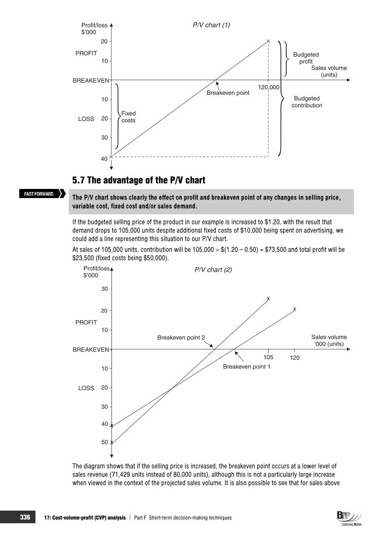
336 17: Cost-volume-profit (CVP) analysis Part F Short-term decision-making techniques
5.7 The advantage of the P/V chart
The P/V chart shows clearly the effect on profit and breakeven point of any changes in selling price, variable cost, fixed cost and/or sales demand.
If the budgeted selling price of the product in our example is increased to $1.20, with the result that demand drops to 105,000 units despite additional fixed costs of $10,000 being spent on advertising, we could add a line representing this situation to our P/V chart.
At sales of 105,000 units, contribution will be 105,000 $(1.20 – 0.50) = $73,500 and total profit will be $23,500 (fixed costs being $50,000).
The diagram shows that if the selling price is increased, the breakeven point occurs at a lower level of sales revenue (71,429 units instead of 80,000 units), although this is not a particularly large increase when viewed in the context of the projected sales volume. It is also possible to see that for sales above
FAST FORWARD

Part F Short-term decision-making techniques 17: Cost-volume-profit (CVP) analysis 337
50,000 units, the profit achieved will be higher (and the loss achieved lower) if the price is $1.20. For sales volumes below 50,000 units the first option will yield lower losses.
The P/V chart is the clearest way of presenting such information; two conventional breakeven charts on one set of axes would be very confusing.
Changes in the variable cost per unit or in fixed costs at certain activity levels can also be easily incorporated into a P/V chart. The profit or loss at each point where the cost structure changes should be calculated and plotted on the graph so that the profit/volume line becomes a series of straight lines.
For example, suppose that in our example, at sales levels in excess of 120,000 units the variable cost per unit increases to $0.60 (perhaps because of overtime premiums that are incurred when production exceeds a certain level). At sales of 130,000 units, contribution would therefore be 130,000 $(1 – 0.60) = $52,000 and total profit would be $12,000.
You may be given a breakeven or PV chart and required to extract the information from it.
Question Profit/volume chart
The profit/volume chart for a single product company is as follows:
Profit($'000)
140
0 500 Sales revenue ($'000)
(60)
Exam focus point

338 17: Cost-volume-profit (CVP) analysis Part F Short-term decision-making techniques
What is the product’s contribution to sales ratio (expressed as a %)?
A 16% B 28% C 40% D 72%
AnswerThe correct answer is C.
The profit/volume graph shows levels of profit at different levels of sales. In order to answer the question, you must determine contribution for $500,000 sales revenue.
Remember that profit = contribution – fixed costs.
When sales revenue = 0, contribution = 0 and the graph shows a loss of $60,000 at zero sales revenue.This means that fixed costs must be $60,000.
Contribution at $500,000 sales revenue = $140,000 (profit) + $60,000 (fixed costs)
= $200,000
Contribution to sales ratio = contribution/sales revenue = ($200,000/$500,000) = 0.4 or 40%
This question appeared in the December 2008 exam and was answered correctly by only one third of students. Most students calculated the profit/sales ratio using the $140,000 shown on the graph and thus selected choice B.
6 Limitations of CVP analysis
Breakeven analysis is a useful technique for managers as it can provide simple and quick estimates. Breakeven charts provide a graphical representation of breakeven arithmetic. Breakeven analysis does, however, have number of limitations.
It can only apply to a single product or a single mix of a group of products A breakeven chart may be time-consuming to prepare It assumes fixed costs are constant at all levels of output. It assumes that variable costs are the same per unit at all levels of output It assumes that sales prices are constant at all levels of output It assumes production and sales are the same (inventory levels are ignored) It ignores the uncertainty in the estimates of fixed costs and variable cost per unit
FAST FORWARD
Exam focus point

Part F Short-term decision-making techniques 17: Cost-volume-profit (CVP) analysis 339
Chapter roundup
Cost-volume– profit (CVP)/breakeven analysis is the study of the interrelationships between costs, volume and profits at various levels of activity.
Breakeven point = Number of units of sale required to breakeven
= unit per onContributi
costsfixed Total
= unit per onContributi
evenbreaktorequiredonContributi
Breakeven point in terms of sales revenue
= ratio C/S
evenbreaktorequiredonContributi
= ratio C/Scosts Fixed
The C/S ratio (or P/V ratio) is a measure of how much contribution is earned from each $1 of sales.
The margin of safety is the difference in units between the budgeted sales volume and the breakevensales volume. It is sometimes expressed as a percentage of the budgeted sales volume. The margin of safety may also be expressed as the difference between the budgeted sales revenue and the breakevensales revenue expressed as a percentage of the budgeted sales revenue.
At the breakeven point, sales revenue = total costs and there is no profit. At the breakeven point totalcontribution = fixed costs.
The target profit is achieved when S = V + F + P. Therefore the total contribution required for a target profit = fixed costs + required profit.
The breakeven point can also be determined graphically using a breakeven chart or a contributionbreakeven chart. These charts show approximate levels of profit or loss at different sales volume levels within a limited range.
The profit/volume (PV) chart is a variation of the breakeven chart which illustrates the relationship of costs and profits to sales and the margin of safety.
The P/V chart shows clearly the effect on profit and breakeven point of any changes in selling price, variable cost, fixed cost and/or sales demand.
Breakeven analysis is a useful technique for managers as it can provide simple and quick estimates. Breakeven charts provide a graphical representation of breakeven arithmetic. Breakeven analysis does, however, have a number of limitations.

340 17: Cost-volume-profit (CVP) analysis Part F Short-term decision-making techniques
Quick quiz 1 What does CVP analysis study?
2 The breakeven point is the ………………….……………..……….. or……..……………………………… …………………. .
3 Use the following to make up three formulae which can be used to calculate the breakeven point.
Contribution per unit
Contribution per unit
Fixed costs
Fixed costs
Contribution required to breakeven
Contribution required to breakeven
C/S ratio
C/S ratio
(a) Breakeven point (sales units) =
or
(b) Breakeven point (sales revenue) =
or
4 The C/S ratio is a measure of how much profit is earned from each $1 of sales.
True
False
5 The margin of safety is the difference in units between the budgeted sales volume and the breakeven sales volume. How is it sometimes expressed?
6 Profits are maximised at the breakeven point.
True
False
7 At the breakeven point, total contribution = …………………………………. .
8 The total contribution required for a target profit = ……………………………………………….. .
9 Give three uses of breakeven charts.

Part F Short-term decision-making techniques 17: Cost-volume-profit (CVP) analysis 341
10 Breakeven charts show approximate levels of profit or loss at different sales volume levels within a limited range. Which of the following are true?
I The sales line starts at the origin II The fixed costs line runs parallel to the vertical axis III Breakeven charts have a horizontal axis showing the sales/output (in value or units) IV Breakeven charts have a vertical axis showing $ for revenues and costs V The breakeven point is the intersection of the sales line and the fixed cost line
A I and II B I and III C I, III and IV D I, III, IV, and V
11 On a breakeven chart, the distance between the breakeven point and the expected (or budgeted) sales, in units, indicates the ………………………………. .
12 Give seven limitations of CVP analysis.
……………………………………………………………………………………………………. ……………………………………………………………………………………………………. ……………………………………………………………………………………………………. ……………………………………………………………………………………………………. ……………………………………………………………………………………………………. ……………………………………………………………………………………………………. …………………………………………………………………………………………………….

342 17: Cost-volume-profit (CVP) analysis Part F Short-term decision-making techniques
Answers to quick quiz 1 The interrelations between costs, volume and profits of a product at various activity levels.
2 The breakeven point is the number of units of sale required to breakeven or the sales revenue required to breakeven.
3 (a) Breakeven point (sales units) = unit per onContributi
costsFixed
or unit per onContributibreakeventorequiredonContributi
(b) Breakeven point (sales revenue) = ratio C/ScostsFixed
or ratio C/S
breakeventorequiredonContributi
4 False. The C/S ratio is a measure of how much contribution is earned from each $1 of sales.
5 As a percentage of the budgeted sales volume.
6 False. At the breakeven point there is no profit.
7 At the breakeven point, total contribution = fixed costs
8 Fixed costs + required profit
9 To plan the production of a company's products To market a company's products To give a visual display of breakeven arithmetic
10 C
11 Margin of safety
12 It can only apply to a single product or a single mix of a group of products. A breakeven chart may be time-consuming to prepare. It assumes fixed costs are constant at all levels of output. It assumes that variable costs are the same per unit at all levels of output. It assumes that sales prices are constant at all levels of output. It assumes production and sales are the same (inventory levels are ignored). It ignores the uncertainty in the estimates of fixed costs and variable cost per unit.
Now try the questions below from the Exam Question Bank
Number Level Marks Time
Q17 MCQ n/a n/a

343
Relevant costing and decision-making
IntroductionManagement at all levels within an organisation take decisions. The overriding requirement of the information that should be supplied by the cost accountant to aid decision making is that of relevance. This chapter therefore begins by looking at the costing technique required in decision-making situations, that of relevant costing, and explains how to decide which costs need taking into account when a decision is being made and which costs do not.
We then go on to see how to apply relevant costing to product mix decisions.
Topic list Syllabus reference
1 Relevant costs F2 (a)-(d)
2 Choice of product (product mix) decisions F3 (a), (b)

344 18: Relevant costing and decision-making Part F Short-term decision-making techniques
Study guide Intellectual level
F2 Relevant costing
(a) Explain the concept of relevant costing 1
(b) Calculate the relevant costs for materials, labour and overheads 2
(c) Calculate the relevant costs associated with non-current assets 1
(d) Explain and apply the concept of opportunity cost 1
F3 Limiting factors
(a) Identify a single limiting factor 1
(b) Determine the optimal production plan where an organisation is restricted by a single limiting factor
2
Exam guide Relevant costing is one of the key syllabus topics for Paper F2. Make sure that you can calculate relevant costs for materials and labour and the deprival value of an asset. Multiple choice questions are a good way of testing your understanding of this subject.
1 Relevant costs
The skills you learn in this section will provide a good basis for the fulfilment of the optional performance objective ‘Prepare financial information for management’ in your PER. One way in which you can demonstrate competence in this area is to prepare management information to assist with decision-making. Being able to identify costs that are relevant to a particular decision is essential to this skill.
1.1 Relevant costs
Relevant costs are future cash flows arising as a direct consequence of a decision.
Relevant costs are future costs Relevant costs are cash flows Relevant costs are incremental costs
Decision making should be based on relevant costs.
(a) Relevant costs are future costs. A decision is about the future and it cannot alter what has been done already. Costs that have been incurred in the past are totally irrelevant to any decision that is being made 'now'. Such costs are past costs or sunk costs.
Costs that have been incurred include not only costs that have already been paid, but also costs that have been committed. A committed cost is a future cash flow that will be incurred anyway, regardless of the decision taken now.
(b) Relevant costs are cash flows. Only cash flow information is required. This means that costs or charges which do not reflect additional cash spending (such as depreciation and notional costs) should be ignored for the purpose of decision-making.
(c) Relevant costs are incremental costs. For example, if an employee is expected to have no other work to do during the next week, but will be paid his basic wage (of, say, $100 per week) for attending work and doing nothing, his manager might decide to give him a job which earns the organisation $40. The net gain is $40 and the $100 is irrelevant to the decision because although it is a future cash flow, it will be incurred anyway whether the employee is given work or not.
FAST FORWARD

Part F Short-term decision-making techniques 18: Relevant costing and decision-making 345
1.2 Avoidable costs
Avoidable costs are costs which would not be incurred if the activity to which they relate did not exist.
One of the situations in which it is necessary to identify the avoidable costs is in deciding whether or not to discontinue a product. The only costs which would be saved are the avoidable costs which are usually the variable costs and sometimes some specific costs. Costs which would be incurred whether or not the product is discontinued are known as unavoidable costs.
1.3 Differential costs and opportunity costs
Relevant costs are also differential costs and opportunity costs.
Differential cost is the difference in total cost between alternatives. An opportunity cost is the value of the benefit sacrificed when one course of action is chosen in
preference to an alternative.
For example, if decision option A costs $300 and decision option B costs $360, the differential cost is $60.
1.3.1 Example: Differential costs and opportunity costs
Suppose for example that there are three options, A, B and C, only one of which can be chosen. The net profit from each would be $80, $100 and $70 respectively.
Since only one option can be selected option B would be chosen because it offers the biggest benefit.
$Profit from option B 100Less opportunity cost (ie the benefit from the most profitable alternative, A) 80Differential benefit of option B 20
The decision to choose option B would not be taken simply because it offers a profit of $100, but because it offers a differential profit of $20 in excess of the next best alternative.
1.4 Controllable and uncontrollable costs We came across the term controllable costs at the beginning of this study text. Controllable costs areitems of expenditure which can be directly influenced by a given manager within a given time span.
As a general rule, committed fixed costs such as those costs arising from the possession of plant, equipment and buildings (giving rise to depreciation and rent) are largely uncontrollable in the short term because they have been committed by longer-term decisions.
Discretionary fixed costs, for example, advertising and research and development costs can be thought of as being controllable because they are incurred as a result of decisions made by management and can be raised or lowered at fairly short notice.
1.5 Sunk costs
A sunk cost is a past cost which is not directly relevant in decision making.
The principle underlying decision accounting is that management decisions can only affect the future.In decision making, managers therefore require information about future costs and revenues which would be affected by the decision under review. They must not be misled by events, costs and revenues in the past, about which they can do nothing.
Key term
FAST FORWARD
FAST FORWARD
346 18: Relevant costing and decision-making Part F Short-term decision-making techniques
Sunk costs, which have been charged already as a cost of sales in a previous accounting period or will be charged in a future accounting period although the expenditure has already been incurred, are irrelevant to decision-making.
1.5.1 Example: Sunk costs
An example of a sunk cost is development costs which have already been incurred. Suppose that a company has spent $250,000 in developing a new service for customers, but the marketing department's most recent findings are that the service might not gain customer acceptance and could be a commercial failure. The decision whether or not to abandon the development of the new service would have to be taken, but the $250,000 spent so far should be ignored by the decision makers because it is a sunk cost.
1.6 Fixed and variable costs
In general, variable costs will be relevant costs and fixed costs will be irrelevant to a decision.
Unless you are given an indication to the contrary, you should assume the following.
Variable costs will be relevant costs. Fixed costs are irrelevant to a decision.
This need not be the case, however, and you should analyse variable and fixed cost data carefully. Do not forget that 'fixed' costs may only be fixed in the short term.
1.6.1 Non-relevant variable costs
There might be occasions when a variable cost is in fact a sunk cost (and therefore a non-relevantvariable cost). For example, suppose that a company has some units of raw material in inventory. They have been paid for already, and originally cost $2,000. They are now obsolete and are no longer used in regular production, and they have no scrap value. However, they could be used in a special job which the company is trying to decide whether to undertake. The special job is a 'one-off' customer order, and would use up all these materials in inventory.
(a) In deciding whether the job should be undertaken, the relevant cost of the materials to the special job is nil. Their original cost of $2,000 is a sunk cost, and should be ignored in the decision.
(b) However, if the materials did have a scrap value of, say, $300, then their relevant cost to the job would be the opportunity cost of being unable to sell them for scrap, ie $300.
1.6.2 Attributable fixed costs
There might be occasions when a fixed cost is a relevant cost, and you must be aware of the distinction between 'specific' or 'directly attributable' fixed costs, and general fixed overheads.
Directly attributable fixed costs are those costs which, although fixed within a relevant range of activity level are relevant to a decision for either of the following reasons.
(a) They could increase if certain extra activities were undertaken. For example, it may be necessary to employ an extra supervisor if a particular order is accepted. The extra salary would be an attributable fixed cost.
(b) They would decrease or be eliminated entirely if a decision were taken either to reduce the scale of operations or shut down entirely.
General fixed overheads are those fixed overheads which will be unaffected by decisions to increase or decrease the scale of operations, perhaps because they are an apportioned share of the fixed costs of items which would be completely unaffected by the decisions. General fixed overheads are not relevant in decision-making.
Exam focus point
FAST FORWARD
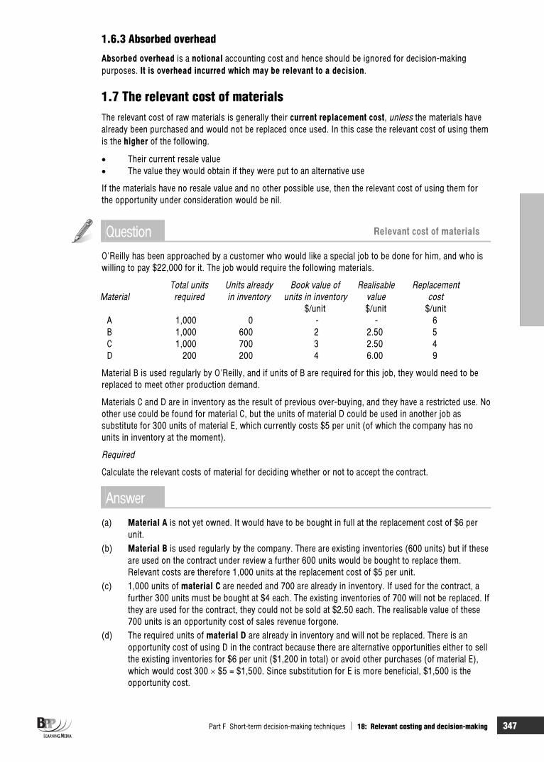
Part F Short-term decision-making techniques 18: Relevant costing and decision-making 347
1.6.3 Absorbed overhead
Absorbed overhead is a notional accounting cost and hence should be ignored for decision-making purposes. It is overhead incurred which may be relevant to a decision.
1.7 The relevant cost of materials The relevant cost of raw materials is generally their current replacement cost, unless the materials have already been purchased and would not be replaced once used. In this case the relevant cost of using them is the higher of the following.
Their current resale value The value they would obtain if they were put to an alternative use
If the materials have no resale value and no other possible use, then the relevant cost of using them for the opportunity under consideration would be nil.
Question Relevant cost of materials
O'Reilly has been approached by a customer who would like a special job to be done for him, and who is willing to pay $22,000 for it. The job would require the following materials.
Total units Units already Book value of Realisable Replacement Material required in inventory units in inventory value cost $/unit $/unit $/unit A 1,000 0 - - 6 B 1,000 600 2 2.50 5 C 1,000 700 3 2.50 4 D 200 200 4 6.00 9
Material B is used regularly by O'Reilly, and if units of B are required for this job, they would need to be replaced to meet other production demand.
Materials C and D are in inventory as the result of previous over-buying, and they have a restricted use. No other use could be found for material C, but the units of material D could be used in another job as substitute for 300 units of material E, which currently costs $5 per unit (of which the company has no units in inventory at the moment).
Required
Calculate the relevant costs of material for deciding whether or not to accept the contract.
Answer(a) Material A is not yet owned. It would have to be bought in full at the replacement cost of $6 per
unit.(b) Material B is used regularly by the company. There are existing inventories (600 units) but if these
are used on the contract under review a further 600 units would be bought to replace them. Relevant costs are therefore 1,000 units at the replacement cost of $5 per unit.
(c) 1,000 units of material C are needed and 700 are already in inventory. If used for the contract, a further 300 units must be bought at $4 each. The existing inventories of 700 will not be replaced. If they are used for the contract, they could not be sold at $2.50 each. The realisable value of these 700 units is an opportunity cost of sales revenue forgone.
(d) The required units of material D are already in inventory and will not be replaced. There is an opportunity cost of using D in the contract because there are alternative opportunities either to sell the existing inventories for $6 per unit ($1,200 in total) or avoid other purchases (of material E), which would cost 300 $5 = $1,500. Since substitution for E is more beneficial, $1,500 is the opportunity cost.

348 18: Relevant costing and decision-making Part F Short-term decision-making techniques
(e) Summary of relevant costs$
Material A (1,000 $6) 6,000
Material B (1,000 $5) 5,000
Material C (300 $4) plus (700 $2.50) 2,950Material D 1,500Total 15,450
Question Relevant material costs
A company regularly uses a material. It currently has 100kg in inventory for which it paid $200. If it were sold it could be sold for $3 per kg. The market price is now $4 per kg. A customer has placed an order that will use 200kg of the material. The relevant cost of the 200kg is:
A $500 B $600 C $700 D $800
AnswerThe material is in regular use and so 200kg will be purchased. The relevant cost is therefore 200 $4 = $800. Answer D.
1.8 The relevant cost of labour The relevant cost of labour, in different situations, is best explained by means of an example.
1.8.1 Example: Relevant cost of labour
LW is currently deciding whether to undertake a new contract. 15 hours of labour will be required for the contract. LW currently produces product L, the standard cost details of which are shown below.
STANDARD COST CARD PRODUCT L
$/unitDirect materials (10kg @ $2) 20Direct labour (5 hrs @ $6) 30
50Selling price 72Contribution 22
(a) What is the relevant cost of labour if the labour must be hired from outside the organisation? (b) What is the relevant cost of labour if LW expects to have 5 hours spare capacity? (c) What is the relevant cost of labour if labour is in short supply?
Solution
(a) Where labour must be hired from outside the organisation, the relevant cost of labour will be the variable costs incurred.
Relevant cost of labour on new contract = 15 hours @ $6 = $90
(b) It is assumed that the 5 hours spare capacity will be paid anyway, and so if these 5 hours are used on another contract, there is no additional cost to LW.
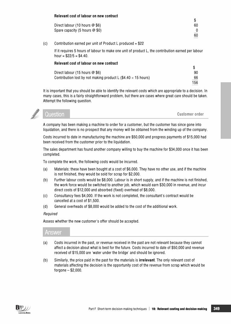
Part F Short-term decision-making techniques 18: Relevant costing and decision-making 349
Relevant cost of labour on new contract $
Direct labour (10 hours @ $6) 60Spare capacity (5 hours @ $0) 0
60
(c) Contribution earned per unit of Product L produced = $22
If it requires 5 hours of labour to make one unit of product L, the contribution earned per labour hour = $22/5 = $4.40.
Relevant cost of labour on new contract $
Direct labour (15 hours @ $6) 90Contribution lost by not making product L ($4.40 15 hours) 66
156
It is important that you should be able to identify the relevant costs which are appropriate to a decision. In many cases, this is a fairly straightforward problem, but there are cases where great care should be taken. Attempt the following question.
Question Customer order
A company has been making a machine to order for a customer, but the customer has since gone into liquidation, and there is no prospect that any money will be obtained from the winding up of the company.
Costs incurred to date in manufacturing the machine are $50,000 and progress payments of $15,000 had been received from the customer prior to the liquidation.
The sales department has found another company willing to buy the machine for $34,000 once it has been completed.
To complete the work, the following costs would be incurred.
(a) Materials: these have been bought at a cost of $6,000. They have no other use, and if the machine is not finished, they would be sold for scrap for $2,000.
(b) Further labour costs would be $8,000. Labour is in short supply, and if the machine is not finished, the work force would be switched to another job, which would earn $30,000 in revenue, and incur direct costs of $12,000 and absorbed (fixed) overhead of $8,000.
(c) Consultancy fees $4,000. If the work is not completed, the consultant's contract would be cancelled at a cost of $1,500.
(d) General overheads of $8,000 would be added to the cost of the additional work.
Required
Assess whether the new customer's offer should be accepted.
Answer(a) Costs incurred in the past, or revenue received in the past are not relevant because they cannot
affect a decision about what is best for the future. Costs incurred to date of $50,000 and revenue received of $15,000 are 'water under the bridge' and should be ignored.
(b) Similarly, the price paid in the past for the materials is irrelevant. The only relevant cost of materials affecting the decision is the opportunity cost of the revenue from scrap which would be forgone – $2,000.

350 18: Relevant costing and decision-making Part F Short-term decision-making techniques
(c) Labour costs$
Labour costs required to complete work 8,000Opportunity costs: contribution forgone by losing other work $(30,000 – 12,000) 18,000Relevant cost of labour 26,000
(d) The incremental cost of consultancy from completing the work is $2,500. $
Cost of completing work 4,000Cost of cancelling contract 1,500Incremental cost of completing work 2,500
(e) Absorbed overhead is a notional accounting cost and should be ignored. Actual overhead incurred is the only overhead cost to consider. General overhead costs (and the absorbed overhead of the alternative work for the labour force) should be ignored.
(f) Relevant costs may be summarised as follows. $ $
Revenue from completing work 34,000Relevant costsMaterials: opportunity cost 2,000Labour: basic pay 8,000 opportunity cost 18,000Incremental cost of consultant 2,500
30,500Extra profit to be earned by accepting the order 3,500
1.9 The relevant cost of an asset
The relevant cost of an asset represents the amount of money that a company would have to receive if it were deprived of an asset in order to be no worse off than it already is. We can call this the deprivalvalue.
The study guide for Paper F2 states that candidates must be able to calculate the relevant costs associated with non-current assets.
The deprival value of an asset is best demonstrated by means of an example.
1.9.1 Example: Deprival value of an asset
A machine cost $14,000 ten years ago. It is expected that the machine will generate future revenues of $10,000. Alternatively, the machine could be scrapped for $8,000. An equivalent machine in the same condition would cost $9,000 to buy now. What is the deprival value of the machine?
SolutionFirstly, let us think about the relevance of the costs given to us in the question.
Cost of machine = $14,000 = past/sunk cost Future revenues = $10,000 = revenue expected to be generated Net realisable value = $8,000 = scrap proceeds Replacement cost = $9,000
When calculating the deprival value of an asset, use the following diagram.
Exam focus point
FAST FORWARD

Part F Short-term decision-making techniques 18: Relevant costing and decision-making 351
LOWER OF
REPLACEMENT HIGHER OF COST ($10,000) ($9,000)
NRV REVENUES($8,000) EXPECTED
($10,000)
Therefore, the deprival value of the machine is the lower of the replacement cost and $10,000. The deprival value is therefore $9,000.
Your exam will use the term 'relevant cost' rather than 'deprival value', but you may find that 'deprival value' is a useful concept to bear in mind when considering a non-current asset.
2 Choice of product (product mix) decisions 2.1 The limiting factor
A limiting factor is a factor which limits the organisation's activities. In a limiting factor situation,contribution will be maximised by earning the biggest possible contribution per unit of limiting factor.
A limiting factor is anything which limits the activity of the entity. This could be the level of demand for its product or it could be one or more scarce resources which limit production to below that level.
Possible limiting factors are:
(a) Sales. There may be a limit to sales demand (b) Labour. There may be a limit to total quantity of labour available or to labour having particular skills (c) Materials. There may be insufficient available materials to produce enough units to satisfy sales
demand(d) Manufacturing capacity. There may not be sufficient machine capacity for the production required
to meet sales demand
One of the more common decision-making problems is a situation where there are not enough resources to meet the potential sales demand, and so a decision has to be made about what mix of products to produce, using what resources there are as effectively as possible.
A limiting factor could be sales if there is a limit to sales demand but any one of the organisation's resources (labour, materials and so on) may be insufficient to meet the level of production demanded.
It is assumed in limiting factor accounting that management wishes to maximise profit and that profit will be maximised when contribution is maximised (given no change in fixed cost expenditure incurred). In other words, marginal costing ideas are applied.
Contribution will be maximised by earning the biggest possible contribution from each unit of limiting factor. For example if grade A labour is the limiting factor, contribution will be maximised by earning the biggest contribution from each hour of grade A labour worked.
The limiting factor decision therefore involves the determination of the contribution earned by each different product from each unit of the limiting factor.
FAST FORWARD
Exam focus point

352 18: Relevant costing and decision-making Part F Short-term decision-making techniques
2.2 Example: Limiting factor AB makes two products, the Ay and the Be. Unit variable costs are as follows.
Ay Be$ $
Direct materials 1 3Direct labour ($3 per hour) 6 3Variable overhead 1 1
8 7
The sales price per unit is $14 per Ay and $11 per Be. During July 20X2 the available direct labour is limited to 8,000 hours. Sales demand in July is expected to be 3,000 units for Ays and 5,000 units for Bes.
Required
Determine the profit-maximising production mix, assuming that monthly fixed costs are $20,000, and that opening inventories of finished goods and work in progress are nil.
SolutionStep 1 Confirm that the limiting factor is something other than sales demand.
Ays Bes TotalLabour hours per unit 2 hrs 1 hr Sales demand 3,000 units 5,000 units Labour hours needed 6,000 hrs 5,000 hrs 11,000 hrs Labour hours available 8,000 hrsShortfall 3,000 hrs
Labour is the limiting factor on production.
Step 2 Identify the contribution earned by each product per unit of limiting factor, that is per labour hour worked.
Ays Bes$ $
Sales price 14 11Variable cost 8 7Unit contribution 6 4Labour hours per unit 2 hrs 1 hrContribution per labour hour (= unit of limiting factor) $3 $4
Although Ays have a higher unit contribution than Bes, two Bes can be made in the time it takes to make one Ay. Because labour is in short supply it is more profitable to make Bes than Ays.
Step 3 Determine the optimum production plan. Sufficient Bes will be made to meet the full sales demand, and the remaining labour hours available will then be used to make Ays.
(a) Hours Hours Priority ofProduct Demand required available manufactureBes 5,000 5,000 5,000 1stAys 3,000 6,000 3,000 (bal) 2nd
11,000 8,000
(b) Hours ContributionProduct Units needed per unit Total
$ $Bes 5,000 5,000 4 20,000Ays 1,500 3,000 6 9,000
8,000 29,000Less fixed costs 20,000Profit 9,000

Part F Short-term decision-making techniques 18: Relevant costing and decision-making 353
In conclusion
(a) Unit contribution is not the correct way to decide priorities. (b) Labour hours are the scarce resource, and therefore contribution per labour hour is the correct
way to decide priorities. (c) The Be earns $4 contribution per labour hour, and the Ay earns $3 contribution per labour hour.
Bes therefore make more profitable use of the scarce resource, and should be manufactured first.
Question Limiting factor 1
The following details relate to three products made by DSF Co.
V A L$ per unit $ per unit $ per unit
Selling price 120 170 176Direct materials 30 40 60Direct labour 20 30 20Variable overhead 10 16 20Fixed overhead 20 32 40
80 118 140
Profit 40 52 36
All three products use the same direct labour and direct materials, but in different quantities.
In a period when the labour used on these products is in short supply, the most and least profitable use of the labour is
Most profitable Least profitableA L V B L A C V A D A L
AnswerThe correct answer is B.
V A L$ $ $
Selling price per unit 120 170 176Variable cost per unit 60 86 100Contribution per unit 60 84 76
Labour cost per unit $20 $30 $20
Contribution per $ of labour $3 $2.80 $3.80
Ranking 2 3 1
Question Limiting factor 2
Jam Co makes two products, the K and the L. The K sells for $50 per unit, the L for $70 per unit. The variable cost per unit of the K is $35, that of the L $40. Each unit of K uses 2 kg of raw material. Each unit of L uses 3 kg of material.
In the forthcoming period the availability of raw material is limited to 2,000 kg. Jam Co is contracted to supply 500 units of K. Maximum demand for the L is 250 units. Demand for the K is unlimited.
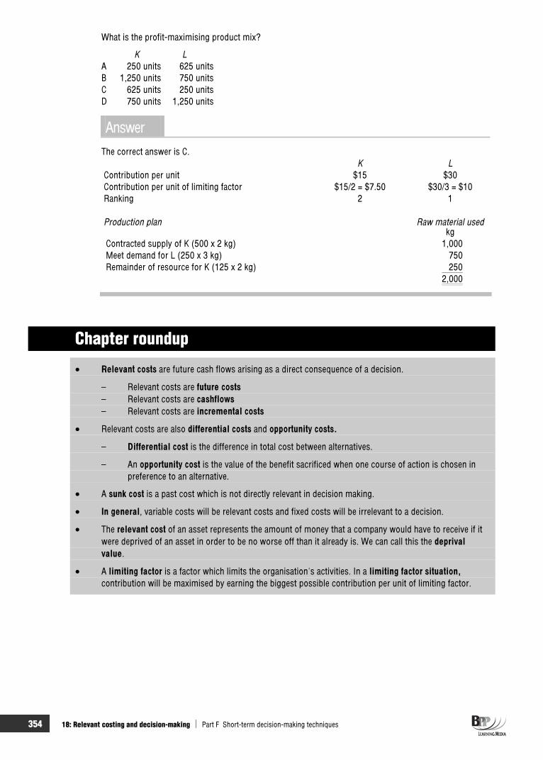
354 18: Relevant costing and decision-making Part F Short-term decision-making techniques
What is the profit-maximising product mix?
K L A 250 units 625 units B 1,250 units 750 units C 625 units 250 units D 750 units 1,250 units
AnswerThe correct answer is C.
K LContribution per unit $15 $30Contribution per unit of limiting factor $15/2 = $7.50 $30/3 = $10 Ranking 2 1
Production plan Raw material used kg
Contracted supply of K (500 x 2 kg) 1,000Meet demand for L (250 x 3 kg) 750Remainder of resource for K (125 x 2 kg) 250
2,000
Chapter roundup
Relevant costs are future cash flows arising as a direct consequence of a decision.
– Relevant costs are future costs – Relevant costs are cashflows– Relevant costs are incremental costs
Relevant costs are also differential costs and opportunity costs.
– Differential cost is the difference in total cost between alternatives.
– An opportunity cost is the value of the benefit sacrificed when one course of action is chosen in preference to an alternative.
A sunk cost is a past cost which is not directly relevant in decision making.
In general, variable costs will be relevant costs and fixed costs will be irrelevant to a decision.
The relevant cost of an asset represents the amount of money that a company would have to receive if it were deprived of an asset in order to be no worse off than it already is. We can call this the deprivalvalue.
A limiting factor is a factor which limits the organisation's activities. In a limiting factor situation,contribution will be maximised by earning the biggest possible contribution per unit of limiting factor.

Part F Short-term decision-making techniques 18: Relevant costing and decision-making 355
Quick quiz 1 Relevant costs are:
(a)(b)(c)(d)(e)
2 Sunk costs are directly relevant in decision making.
True
False
3 The following information relates to machine Z.
Purchase price = $7,000
Expected future revenues = $5,000
Scrap value = $4,000
Replacement cost = $4,500
Complete the following diagram in order to calculate the relevant cost of machine Z.
LOWER OF
REPLACEMENT HIGHER OF COST
NRV REVENUES
The relevant cost of machine Z is ………………………………………………………………………
4 A limiting factor is a factor which ……………………………………………………………………….
5 A sunk cost is:
A a cost committed to be spent in the current period B a cost which is irrelevant for decision making C a cost connected with oil exploration in the North Sea D a cost unaffected by fluctuations in the level of activity

356 18: Relevant costing and decision-making Part F Short-term decision-making techniques
Answers to quick quiz 1 (a) Future costs
(b) Cash flows (c) Incremental costs (d) Differential costs (e) Opportunity costs
2 False
3
LOWER OF
REPLACEMENT HIGHER OFCOST
NRV REVENUES
$4,500
$5,000
$5,000$4,000
$4,500
The relevant cost of machine Z is $4,500.
4 Limits the organisation's activities.
5 B
Now try the questions below from the Exam Question Bank
Number Level Marks Time
Q18 MCQ/OTQ n/a n/a
357
Linearprogramming
IntroductionWe are now going to look at a decision-making technique which involves allocating resources in order to achieve the best results. The name 'linearprogramming' sounds rather formidable and the technique can get very complicated. Don't worry though: you are only expected to be able to analyse the simplest examples.
Topic list Syllabus reference
1 The problem F3 (a), (b)
2 Formulating the problem F3 (c)
3 Graphing the model F3 (d)
4 Finding the best solution F3 (c)
5 The graphical method using simultaneous equations F3 (e)

358 19: Linear programming Part F Short-term decision-making techniques
Study guide Intellectual level
F3 Limiting factors
(a) Identify a single limiting factor 1
(b) Determine the optimal production plan where an organisation is restricted by a single limiting factor
2
(c) Formulate a linear programming problem involving two variables 1
(d) Determine the optimal solution to a linear programming problem using a graphical approach
1
(e) Use simultaneous equations where appropriate, in the solution of a linear programming problem
1
Exam guide The Pilot paper has four questions on this part of the syllabus. Make sure you understand both the graphical approach and the method using simultaneous equations.
Remember to refer to the introductory chapter ‘Basic maths’ if you are having difficulties with this chapter – sections 6 - 9 will be particularly useful.
1 The problem
A limiting factor limits the organisation's production. It could be a limited supply of labour, inventory, machine hours or some other factor. The production plan must aim to maximise the contribution per unit of limiting factor.
A typical business problem is to decide how a company should divide up its production among the various types of product it manufactures in order to obtain the maximum possible profit. A business cannot simply aim to produce as much as possible because there will be limitations or constraints withinwhich the production must operate. Such constraints could be one or more of the following.
Limited quantities of raw materials available A fixed number of man-hours per week for each type of worker Limited machine hours
Moreover, since the profits generated by different products vary, it may be better not to produce any of a less profitable line, but to concentrate all resources on producing the more profitable ones. On the other hand limitations in market demand could mean that some of the products produced may not be sold.
Refer back to Chapter 18 for simple production planning. In this chapter we look at the approach using linear programming.
FAST FORWARD

Part F Short-term decision-making techniques 19: Linear programming 359
2 Formulating the problem
Linear programming is a technique for solving problems of profit maximisation or cost minimisation and resource allocation. 'Programming' has nothing to do with computers: the word is simply used to denote a series of events.
Linear programming, at least at this fairly simple level, is a technique that can be carried out in a fairly 'handle turning' manner once you have got the basic ideas sorted out. The steps involved are as follows.
1 Define variables 5 Establish feasible region 2 Establish constraints 6 Add iso-profit/contribution line 3 Construct objective function 7 Determine optimal solution 4 Graph constraints
Let us imagine that B makes just two models, the Super and the Deluxe, and that the only constraint facedby the company is that monthly machine capacity is restricted to 400 hours. The Super requires 5 hours of machine time per unit and the Deluxe 1.5 hours. Government restrictions mean that the maximum number of units that can be sold each month is 150, that number being made up of any combination of the Super and the Deluxe.
Let us now work through the steps involved in setting up a linear programming model.
Step 1 Define variables
What are the quantities that the company can vary? Obviously not the number of machine hours or the maximum sales, which are fixed by external circumstances beyond the company's control. The only things which it can determine are the number of each type of unit to manufacture. It is these numbers which have to be determined in such a way as to get the maximum possible profit. Our variables will therefore be as follows.
Let x = the number of units of the Super manufactured. Let y = the number of units of the Deluxe manufactured.
Step 2 Establish constraints
Having defined these two variables we can now translate the two constraints into inequalities involving the variables.
Let us first consider the machine hours constraint. Each Super requires 5 hours of machine time. Producing five Supers therefore requires 5 5 = 25 hours of machine time and, more generally, producing x Supers will require 5x hours. Likewise producing y Deluxes will require 1.5y hours. The total machine hours needed to make x Supers and y Deluxes is 5x + 1.5y. We know that this cannot be greater than 400 hours so we arrive at the following inequality.
5x + 1.5y 400
We can obtain the other inequality more easily. The total number of Supers and Deluxes made each month is x + y but this has to be less than 150 due to government restrictions. The sales order constraint is therefore as follows.
x + y 150
Non-negativity
The variables in linear programming models should usually be non-negative in value. In this example, for instance, you cannot make a negative number of units and so we need the following constraints.
x 0; y 0
Do not forget these non-negativity constraints when formulating a linear programming model.
FAST FORWARD

360 19: Linear programming Part F Short-term decision-making techniques
Step 3 Construct objective function
We have yet to introduce the question of profits. Let us assume that the profit on each model is as follows.
$Super 100 Deluxe 200
The objective of B is to maximise profit and so the function to be maximised is as follows.
Profit (P) = 100x + 200y
The problem has now been reduced to the following four inequalities and one equation.
5x + 1.5y 400 x + y 150 x 0 y 0 P = 100x + 200y
Have you noticed that the inequalities are all linear expressions? If plotted on a graph, they would all give straight lines. This explains why the technique is called linearprogramming and also gives a hint as to how we should proceed with trying to find the solution to the problem.
Question Constraints
Patel manufactures two products, X and Y, in quantities x and y units per week respectively. The contribution is $60 per X and $70 per Y. For practical reasons, no more than 100 Xs can be produced per week. If Patel plc uses linear programming to determine a profit-maximising production policy and on the basis of this information, which one of the following constraints is correct?
A x 60 B y 100 C x 100 D 60x + 70y 100
AnswerThe correct answer is C because the question states that the number of Xs produced cannot exceed 100 and so x 100.
Option A has no immediate bearing on the number of units of X produced which must be 100. ($60 represents the contribution per unit of X).
We have no information on the production volume of Product Y and option B is therefore incorrect.
The contribution earned per week is given by 60x + 70y but we have no reason to suppose that this must be less than or equal to 100. Option D is therefore incorrect.
Students often have problems with constraints of the style 'the quantity of one type must not exceed twice that of the other'. This can be interpreted as follows: the quantity of one type (say X) must not exceed (must be less than or equal to) twice that of the other (2Y) (ie X 2Y).
We have looked at how to formulate a problem and in the next section we will look at solving a problem using graphs.
Exam focus point

Part F Short-term decision-making techniques 19: Linear programming 361
3 Graphing the model A graphical solution is only possible when there are two variables in the problem. One variable is represented by the x axis and one by the y axis of the graph. Since non-negative values are not usually allowed, the graph shows only zero and positive values of x and y.
A linear equation with one or two variables is shown as a straight line on a graph. Thus y = 6 would be shown as follows.
y = 6
x
6
y
If the problem included a constraint that y could not exceed 6, the inequality y 6 would be represented by the shaded area of the graph below.
The equation 4x + 3y = 24 is also a straight line on a graph. To draw any straight line, we need only to plot two points and join them up. The easiest points to plot are the following.
(a) x = 0 (in this example, if x = 0, 3y = 24, y = 8) (b) y = 0 (in this example, if y = 0, 4x = 24, x = 6)
By plotting the points, (0, 8) and (6, 0) on a graph, and joining them up, we have the line for 4x + 3y = 24.
x
y
4x + 3y = 248
6
If we had a constraint 4x + 3y 24, any combined value of x and y within the shaded area below (on or below the line) would satisfy the constraint.
FAST FORWARD

362 19: Linear programming Part F Short-term decision-making techniques
x
y
4x + 3y = 24
P
Q
Feasiblearea
For example, at point P where (x = 2, y = 2) 4x + 3y = 14 which is less than 24; and at point Q where x = 5.5, y = 2/3, 4x + 3y = 24. Both P and Q lie within the feasible area (the area where the inequality is satisfied, also called the feasible region). A feasible area enclosed on all sides may also be called a feasible polygon.
The inequalities y 6, x 6 and 4x + 3y 24, would be shown graphically as follows.
xx x
y y y
4x + 3y = 24
Feasiblearea
Feasiblearea
Feasiblearea
y = 6 x = 6
When there are several constraints, the feasible area of combinations of values of x and y must be an area where all the inequalities are satisfied.
Thus, if y 6 and 4x + 3y 24 the feasible area would be the shaded area in the graph following.
RS
8
6
Ty = 6
x
y
4x + 3y = 24Feasible
area
0
6
(a) Point R (x = 0.75, y = 7) is not in the feasible area because although it satisfies the inequality 4x + 3y 24, it does not satisfy y 6.
(b) Point T (x = 5, y = 6) is not in the feasible area, because although it satisfies the inequality y 6, it does not satisfy 4x + 3y 24.
(c) Point S (x = 1.5, y = 6) satisfies both inequalities and lies just on the boundary of the feasible area since y = 6 exactly, and 4x + 3y = 24. Point S is thus at the intersection of the two equation lines.
Similarly, if y 6 and 4x + 3y 24 but x 6, the feasible area would be the shaded area in the graph below.

Part F Short-term decision-making techniques 19: Linear programming 363
8
6
y = 6
x
y
4x + 3y = 24
Feasiblearea x = 6
6
0
Question Feasible region
Draw the feasible region which arises from the constraints facing B Co (see Section 2).
AnswerIf 5x + 1.5y = 400, then if x = 0, y = 267 and if y = 0, x = 80. If x + y = 150, then if x = 0, y = 150 and if y = 0, x = 150
050 100 150 200 250 x Number of Supers
Number ofDeluxes 300
y
100
200 5x + 1.5y = 400
x + y = 150
FEASIBLEAREA
Question Linear programming problem
In a linear programming problem, one of the constraints is given by 2x 3y. Which of the following statements about the graphical presentation of this constraint is correct?
I The constraint line passes through the point x = 2, y = 3. II The constraint line passes through the origin. III The constraint line passes through the point x = 3, y = 2. IV The region below the constraint line is part of the feasible area.
A I and II only B I and III only C II and III only D II, III and IV only
AnswerWhen x = 0 then y must also equal 0, therefore statement II is correct. When x = 3, 6 = 3y and hence y = 2, therefore statement III is correct. Statements II and III are correct and therefore option C is the right answer. Statement I is incorrect since when x = 2, 4 = 3y and y = 1.33 and y does not equal 3 when x = 2. Statement IV is incorrect since 3y is greater than 2x above the line, not below it.

364 19: Linear programming Part F Short-term decision-making techniques
4 Finding the best solution 4.1 Introduction Having found the feasible region (which includes all the possible solutions to the problem) we need to find which of these possible solutions is 'best' in the sense that it yields the maximum possible profit. We could do this by finding out what profit each of the possible solutions would give, and then choosing as our 'best' combination the one for which the profit is greatest.
Consider, however, the feasible region of the problem faced by B Co (see the solution to the question entitled Feasible region). Even in such a simple problem as this, there are a great many possible solution points within the feasible area. Even to write them all down would be a time consuming process and also an unnecessary one, as we shall see.
4.2 Example: Finding the best solution Let us look again at the graph of B's problem.
Consider, for example, the point A at which 40 Supers and 80 Deluxes are being manufactured. This will yield a profit of ((40 100) + (80 200)) = $20,000. We would clearly get more profit at point B, where the same number of Deluxes are being manufactured but where the number of Supers being manufactured has increased by five, or from point C where the same number of Supers but 10 more Deluxes are manufactured. This argument suggests that the 'best' solution is going to be a point on the edge of the feasible area rather than in the middle of it.
0 50 100 150 200 250 xNumber
of Supers
Number ofDeluxes 300
y
100
200 5x + 1.5y = 400
x + y = 150
FEASIBLEAREA
CA B
This still leaves us with quite a few points to look at but there is a way we can narrow down the candidates for the best solution still further. Suppose that B Co wish to make a profit of $10,000. The company could sell the following combinations of Supers and Deluxes.
(a) 100 Super, no Deluxe (b) No Super, 50 Deluxe (c) A proportionate mix of Super and Deluxe, such as 80 Super and 10 Deluxe or 50 Super and 25
Deluxe
The possible combinations of Supers and Deluxes required to earn a profit of $10,000 could be shown by the straight line 100x + 200y = 10,000.
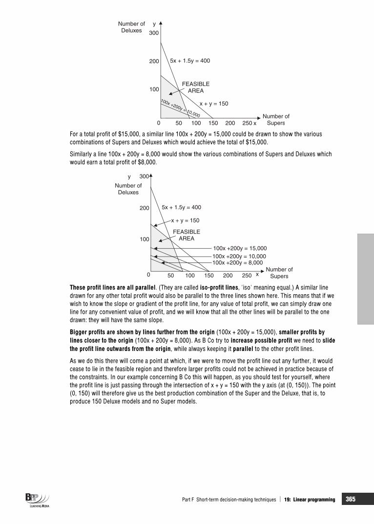
Part F Short-term decision-making techniques 19: Linear programming 365
0 50 100 150 200 250 xNumber of
Supers
Number ofDeluxes 300
y
100
200 5x + 1.5y = 400
x + y = 150100x +200y = 10,000
FEASIBLEAREA
For a total profit of $15,000, a similar line 100x + 200y = 15,000 could be drawn to show the various combinations of Supers and Deluxes which would achieve the total of $15,000.
Similarly a line 100x + 200y = 8,000 would show the various combinations of Supers and Deluxes which would earn a total profit of $8,000.
0 50 100 150 200 250 xNumber of
Supers
Number ofDeluxes
300y
100
200 5x + 1.5y = 400
x + y = 150
100x +200y = 15,000100x +200y = 10,000100x +200y = 8,000
FEASIBLEAREA
These profit lines are all parallel. (They are called iso-profit lines, 'iso' meaning equal.) A similar line drawn for any other total profit would also be parallel to the three lines shown here. This means that if we wish to know the slope or gradient of the profit line, for any value of total profit, we can simply draw one line for any convenient value of profit, and we will know that all the other lines will be parallel to the one drawn: they will have the same slope.
Bigger profits are shown by lines further from the origin (100x + 200y = 15,000), smaller profits by lines closer to the origin (100x + 200y = 8,000). As B Co try to increase possible profit we need to slidethe profit line outwards from the origin, while always keeping it parallel to the other profit lines.
As we do this there will come a point at which, if we were to move the profit line out any further, it would cease to lie in the feasible region and therefore larger profits could not be achieved in practice because of the constraints. In our example concerning B Co this will happen, as you should test for yourself, where the profit line is just passing through the intersection of x + y = 150 with the y axis (at (0, 150)). The point (0, 150) will therefore give us the best production combination of the Super and the Deluxe, that is, to produce 150 Deluxe models and no Super models.

366 19: Linear programming Part F Short-term decision-making techniques
4.3 Example: A maximisation problem Brunel manufactures plastic-covered steel fencing in two qualities, standard and heavy gauge. Both products pass through the same processes, involving steel-forming and plastic bonding.
Standard gauge fencing sells at $18 a roll and heavy gauge fencing at $24 a roll. Variable costs per roll are $16 and $21 respectively. There is an unlimited market for the standard gauge, but demand for the heavy gauge is limited to 1,300 rolls a year. Factory operations are limited to 2,400 hours a year in each of the two production processes.
Processing hours per roll Gauge Steel-forming Plastic-bondingStandard 0.6 0.4Heavy 0.8 1.2
What is the production mix which will maximise total contribution and what would be the total contribution?
Solution(a) Let S be the number of standard gauge rolls per year.
Let H be the number of heavy gauge rolls per year.
The objective is to maximise 2S + 3H (contribution) subject to the following constraints.
0.6S + 0.8H 2,400 (steel-forming hours) 0.4S +1.2H 2,400 (plastic-bonding hours) H 1,300 (sales demand) S, H 0
Note that the constraints are inequalities, and are not equations. There is no requirement to use up the total hours available in each process, nor to satisfy all the demand for heavy gauge rolls.
(b) If we take the production constraint of 2,400 hours in the steel-forming process
0.6S + 0.8H 2,400
it means that since there are only 2,400 hours available in the process, output must be limited to a maximum of:
(i)6.0
400,2 = 4,000 rolls of standard gauge;
(ii)8.0
400,2 = 3,000 rolls of heavy gauge; or
(iii) a proportionate combination of each.
This maximum output represents the boundary line of the constraint, where the inequality becomes the equation
0.6S + 0.8H = 2,400.
(c) The line for this equation may be drawn on a graph by joining up two points on the line (such as S = 0, H = 3,000; H = 0, S = 4,000).
(d) The other constraints may be drawn in a similar way with lines for the following equations.
0.4S + 1.2H = 2,400 (plastic-bonding) H = 1,300 (sales demand)

Part F Short-term decision-making techniques 19: Linear programming 367
(e)
0
3,000
4,000
6,000
2,000 3,000
H = 1,300
0.6S + 0.8H = 2,400
0.4S+
1.2H=
2,400
2S +3H = 6,000
A
BC
D H
S
To satisfy all the constraints simultaneously, the values of S and H must lie on or below each constraint line. The outer limits of the feasible polygon are the lines, but all combined values of S and H within the shaded area are feasible solutions.
(f) The next step is to find the optimal solution, which maximises the objective function. Since the objective is to maximise contribution, the solution to the problem must involve relatively high values (within the feasible polygon) for S, or H or a combination of both.
If, as is likely, there is only one combination of S and H which provides the optimal solution, this combination will be one of the outer corners of the feasible polygon. There are four such corners, A, B, C and D. However, it is possible that any combination of values for S and H on the boundary line between two of these corners might provide solutions with the same total contribution.
(g) To solve the problem we establish the slope of the iso-contribution lines, by drawing a line for any one level of contribution. In our solution, a line 2S + 3H = 6,000 has been drawn. (6,000 was chosen as a convenient multiple of 2 and 3). This line has no significance except to indicate the slope, or gradient, of every iso-contribution line for 2S + 3H.
Using a ruler to judge at which corner of the feasible polygon we can draw an iso– contribution line which is as far to the right as possible, (away from the origin) but which still touches the feasible polygon.
(h) This occurs at corner B where the constraint line 0.4S + 1.2H = 2,400 crosses with the constraint line 0.6S + 0.8H = 2,400. At this point, there are simultaneous equations, from which the exact values of S and H may be calculated.
0.4S + 1.2H = 2,400 (1) 0.6S + 0.8H = 2,400 (2) 1.2S + 3.6H = 7,200 (3) ((1) 3) 1.2S + 1.6H = 4,800 (4) ((2) 2) 2H = 2,400 (5) ((3) – (4)) H = 1,200 (6)
Substituting 1,200 for H in either equation, we can calculate that S = 2,400.
The contribution is maximised where H = 1,200, and S = 2,400. Contribution Total
Units per unit contribution $ $
Standard gauge 2,400 2 4,800Heavy gauge 1,200 3 3,600
8,400

368 19: Linear programming Part F Short-term decision-making techniques
Question Linear programming model
The Dervish Chemical Company operates a small plant. Operating the plant requires two raw materials, A and B, which cost $5 and $8 per litre respectively. The maximum available supply per week is 2,700 litres of A and 2,000 litres of B.
The plant can operate using either of two processes, which have differing contributions and raw materials requirements, as follows.
Raw materials consumed Contribution Process (litres per processing hour) per hour
A B $ 1 20 10 70 2 30 20 60
The plant can run for 120 hours a week in total, but for safety reasons, process 2 cannot be operated for more than 80 hours a week.
Formulate a linear programming model, and then solve it, to determine how many hours process 1 should be operated each week and how many hours process 2 should be operated each week.
AnswerThe decision variables are processing hours in each process. If we let the processing hours per week for process 1 be P1 and the processing hours per week for process 2 be P 2 we can formulate an objective and constraints as follows.
The objective is to maximise 70P1 + 60P 2 , subject to the following constraints.
20P1 + 30P2 2,700 (material A supply) 10P1 + 20P2 2,000 (material B supply) P2 80 (maximum time for P2)P1 + P2 120 (total maximum time) P1 , P2 0 (non-negativity)
0
60
120135
200P1
P1 P2 = 120
+
AB
CD
P = 802
Iso-contribution line
70P +60P = 4,200
12
70 80 90 100 120 P2
10P+20P
=2,000
1
2
20P +30P = 2,700
1
2
The feasible area is ABCDO. The optimal solution, found by moving the iso-contribution line outwards, is at point A, where P1 = 120 and P 2 = 0. Total contribution would be 120 70 = $8,400 a week.

Part F Short-term decision-making techniques 19: Linear programming 369
4.4 Multiple solutionsIt is possible that the optimum position might lie, not at a particular corner, but all along the length of one of the sides of the feasibility polygon. This will occur if the iso-contribution line is exactly parallel to one of the constraint lines.
If this happens then there is no one optimum solution but a range of optimum solutions. All of these will maximise the objective function at the same level. However, any value of the decision variables that happens to satisfy the constraint between the points where the constraint line forms part of the feasibility region would produce this optimum level of contribution.
4.5 Minimisation problems in linear programming Although decision problems with limiting factors usually involve the maximisation of contribution, there may be a requirement to minimise costs. A graphical solution, involving two variables, is very similar to that for a maximisation problem, with the exception that instead of finding a contribution line touching the feasible area as far away from the origin as possible, we look for a total cost line touching the feasible area as close to the origin as possible.
4.5.1 Example: A minimisation problem
Claire Speke Co has undertaken a contract to supply a customer with at least 260 units in total of two products, X and Y, during the next month. At least 50% of the total output must be units of X. The products are each made by two grades of labour, as follows. X Y Hours HoursGrade A labour 4 6Grade B labour 4 2Total 8 8
Although additional labour can be made available at short notice, the company wishes to make use of 1,200 hours of Grade A labour and 800 hours of Grade B labour which has already been assigned to working on the contract next month. The total variable cost per unit is $120 for X and $100 for Y.
Claire Speke Ltd wishes to minimise expenditure on the contract next month. How much of X and Y should be supplied in order to meet the terms of the contract?
Solution(a) Let the number of units of X supplied be x, and the number of units of Y supplied be y.
The objective is to minimise 120x + 100y (costs), subject to the following constraints.
x + y 260 (supply total) x 0.5 (x + y) (proportion of x in total) 4x + 6y 1,200 (Grade A labour) 4x + 2y 800 (Grade B labour) x, y 0
The constraint x 0.5 (x + y) needs simplifying further.
x 0.5 (x + y) 2x x + y x y
In a graphical solution, the line will be x = y. Check this carefully in the following diagram.

370 19: Linear programming Part F Short-term decision-making techniques
0
200
260
360
400
200 300 400
y
x
4x+ 2y
=800x
+y
=260
4x + 6y = 1,200
120x +100y = 36,000
x=
y
Feasiblearea
260
(b) The cost line 120x + 100y = 36,000 has been drawn to show the slope of every cost line 120x + 100 y. Costs are minimised where a cost line touches the feasible area as close as possible to the origin of the graph. This occurs where the constraint line 4x + 2y = 800 crosses the constraint line x + y = 260. This point is found as follows.
x + y = 260 (1) 4x + 2y = 800 (2) 2x + y = 400 (3) ((2) ÷ 2) x = 140 (4) ((3) – (1)) y = 120 (5)
(c) Costs will be minimised by supplying the following. Unit cost Total cost
$ $140 units of X 120 16,800 120 units of Y 100 12,000
28,800
The proportion of units of X in the total would exceed 50%, and demand for Grade A labour would exceed the 1,200 hours minimum.
4.6 The use of simultaneous equations You might think that a lot of time could be saved if we started by solving the simultaneous equations in a linear programming problem and did not bother to draw the graph.
Certainly, this procedure may give the right answer, but in general, it is not recommended until you have shown graphically which constraints are effective in determining the optimal solution. To illustrate this point, consider the following graph.
Feasible area
A BC
D
E0
y
x

Part F Short-term decision-making techniques 19: Linear programming 371
No figures have been given on the graph but the feasible area is OABCDE. When solving this problem, we would know that the optimum solution would be at one of the corners of the feasible area. We need to work out the profit at each of the corners of the feasible area and pick the one where the profit is greatest.
Once the optimum point has been determined graphically, simultaneous equations can be applied to find the exact values of x and y at this point.
5 The graphical method using simultaneous equations
The optimal solution can also be found using simultaneous equations.
Simultaneous equations are covered in section 9 of the introductory chapter ‘Basic maths’.
5.1 Example: using simultaneous equations An organisation manufactures plastic-covered steel fencing in two qualities: standard and heavy gauge. Both products pass through the same processes involving steel forming and plastic bonding.
The standard gauge sells at $15 a roll and the heavy gauge at $20 a roll. There is an unlimited market for the standard gauge but outlets for the heavy gauge are limited to 13,000 rolls a year. The factory operations of each process are limited to 2,400 hours a year. Other relevant data is given below.
Variable costs per roll Direct Direct Direct
material wages expense $ $ $Standard 5 7 1 Heavy 7 8 2
Processing hours per 100 rolls Steel Plastic
forming bonding Hours HoursStandard 6 4Heavy 8 12
Required
Calculate the allocation of resources and hence the production mix which will maximise total contribution.
SolutionStep 1 Define variables
Let the number of rolls of standard gauge to be produced be x and the number of rolls of heavy gauge be y.
Step 2 Establish objective function Standard gauge produces a contribution of $2 per roll ($15 – $(5 + 7 + 1)) and heavy gauge a contribution of $3 ($20 – $(7 + 8 + 2)).
Therefore the objective is to maximise contribution (C) = 2x + 3y subject to the constraints below.
Step 3 Establish constraints The constraints are as follows.
0.06x + 0.08y 2,400 (steel forming hours) 0.04x + 0.12y 2,400 (plastic bonding hours)
y 13,000 (demand for heavy gauge) x, y 0 (non-negativity)
FAST FORWARD

372 19: Linear programming Part F Short-term decision-making techniques
Step 4 Graph problem The graph of the problem can now be drawn.
Step 5 Define feasible area The combinations of x and y that satisfy all three constraints are represented by the area OABCD.
Step 6 Determine optimal solution Which combination will maximise contribution? Obviously, the more units of x and y, the bigger the contribution will be, and the optimal solution will be at point B, C or D. It will not be at A, since at A, y = 13,000 and x = 0, whereas at B, y = 13,000 (the same) and x is greater than zero.
Using simultaneous equations to calculate the value of x and y at each of points B, C and D, and then working out total contribution at each point from this, we can establish the contribution-maximising product mix.
Point B y = 13,000 (1)
0.04x + 0.12y = 2,400 (2) (Plastic forming hours) 0.12y = 1,560 (3) ((1) 0.12) (13,000 0.12)
0.04x = 840 (4) ((2) – (3)) (2,400 – 1,560 x = 21,000 (5) (840 0.04)
Total contribution = (21,000 $2) + (13,000 $3) = $81,000.
Note. At Point B we can see from the graph that y =13,000, so we only need to find x. At Point C we have to find x and y.
Point C
0.06x + 0.08y = 2,400 (1) (Steel forming hours) 0.04x + 0.12y = 2,400 (2) (Plastic bonding hours) 0.12x + 0.16y = 4,800 (3) ((1) 2) 0.12x + 0.36y = 7,200 (4) ((2) 3)
0.2y = 2,400 (5) ((4) – (3)) y = 12,000 (6)
0.06x + 960 = 2,400 (7) (substitute in (1)) (960 = 0.08y) x = 24,000 (8)
Total contribution = (24,000 $2) + (12,000 $3) = $84,000.
Here we produce two equations in which the value of X is the same. This enables us to calculate Y
Part F Short-term decision-making techniques 19: Linear programming 373
Point D
Total contribution = 40,000 $2 = $80,000.
Comparing B, C and D, we can see that contribution is maximised at C, by making 24,000 rolls of standard gauge and 12,000 rolls of heavy gauge, to earn a contribution of $84,000.
In exam questions involving the graphical method, you will not be expected to draw a complete graph. However, you may be given an incomplete graph that you may be required to complete to gain the marks available.
Chapter roundup
A limiting factor limits the organisation's production, It could be a limited supply of labour, inventory, machine hours or some other factor. The production plan must aim to maximise the contribution per unit of limiting factor.
Linear programming is a technique for solving problems of profit maximisation or cost minimisation and resource allocation. 'Programming' has nothing to do with computers: the word is simply used to denote a series of events.
Linear programming, at least at this fairly simple level, is a technique that can be carried out in a fairly 'handle-turning' manner once you have got the basic ideas sorted out. The steps involved are as follows.
1 Define variables 5 Establish feasible region 2 Establish constraints 6 Add iso-profit/contribution line 3 Construct objective function 7 Determine optimal solution 4 Graph constraints
A graphical solution is only possible when there are two variables in the problem. One variable is represented by the x axis and one by the y axis of the graph. Since non-negative values are not usually allowed, the graph only shows zero and positive values of x and y.
The optimal solution can also be found using simultaneous equations.
Exam focus point

374 19: Linear programming Part F Short-term decision-making techniques
Quick quiz 1 What are the three main steps involved in setting up a linear programming model?
Step 1. ……………………..
Step 2. ……………………..
Step 3. …………………..
2 Draw the inequality 4x + 3y 24 on the graph below.
x
y
3 A feasible area enclosed on all sides may also be called a ………………………….. .
4 How does the graphical solution of minimisation problems differ from that of maximisation problems?
5 The graphical method cannot be used when there are more than two decision variables.
True
False
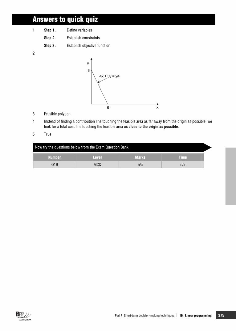
Part F Short-term decision-making techniques 19: Linear programming 375
Answers to quick quiz 1 Step 1. Define variables
Step 2. Establish constraints
Step 3. Establish objective function
2
x
y
4x + 3y = 24
8
6
3 Feasible polygon.
4 Instead of finding a contribution line touching the feasible area as far away from the origin as possible, we look for a total cost line touching the feasible area as close to the origin as possible.
5 True
Now try the questions below from the Exam Question Bank
Number Level Marks Time
Q19 MCQ n/a n/a

376 19: Linear programming Part F Short-term decision-making techniques

377
Exam question andanswer bank

378

Exam question bank 379
1 Information for management (a) Which of the following statements is/are true?
I Information is the raw material for data processing II External sources of information include an organisation's financial accounting records III The main objective of a non-profit making organisation is usually to provide goods and services
A I and III only C II and III only B I, II and III D III only (2 marks)
(b) Which of the following statements is not true?
A Management accounts detail the performance of an organisation over a defined period and the state of affairs at the end of that period
B There is no legal requirement to prepare management accounts C The format of management accounts is entirely at management discretion (1 mark)
(c) Which of the following could higher level management carry out?
A taking long-term decisions B taking short-term decisions C taking long-term and short-term decisions (1 mark)
(d) Which of the following statements is not correct?
A Financial accounting information can be used for internal reporting purposes B Routine information can be used to make decisions regarding both the long term and the
short term C Management accounting provides information relevant to decision making, planning,
control and evaluation of performances D Cost accounting can only be used to provide inventory valuations for internal reporting
(2 marks) (e) Which of the following is not part of the planning stage in the decision-making process? A Deciding on the optimal way in which an objective might be achieved B Identifying ways which might contribute to the achievement of specified objectives C Obtaining data about actual results D Identifying goals or objectives (2 marks)
2 Cost classification (a) Which of the following items might be a suitable cost unit within the accounts payable department
of a company?
(i) Postage cost (iii) Supplier account (ii) Invoice processed
A Item (i) only C Item (iii) only B Item (ii) only D Items (ii) and (iii) only (2 marks)
(b) Which of the following are direct expenses?
(i) The cost of special designs, drawing or layouts (ii) The hire of tools or equipment for a particular job (iii) Salesman's wages (iv) Rent, rates and insurance of a factory
A (i) and (ii) C (i) and (iv) B (i) and (iii) D (iii) and (iv) (2 marks)
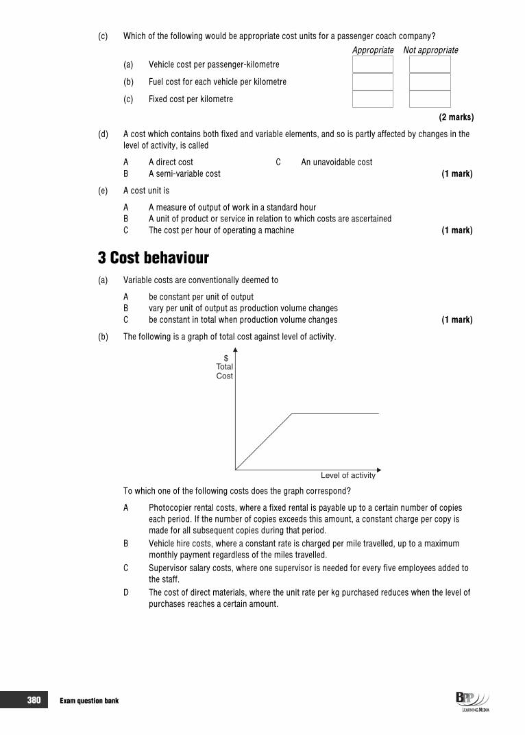
380 Exam question bank
(c) Which of the following would be appropriate cost units for a passenger coach company?
Appropriate Not appropriate
(a) Vehicle cost per passenger-kilometre
(b) Fuel cost for each vehicle per kilometre
(c) Fixed cost per kilometre
(2 marks)
(d) A cost which contains both fixed and variable elements, and so is partly affected by changes in the level of activity, is called
A A direct cost C An unavoidable cost B A semi-variable cost (1 mark)
(e) A cost unit is
A A measure of output of work in a standard hour B A unit of product or service in relation to which costs are ascertained C The cost per hour of operating a machine (1 mark)
3 Cost behaviour (a) Variable costs are conventionally deemed to
A be constant per unit of output B vary per unit of output as production volume changes C be constant in total when production volume changes (1 mark)
(b) The following is a graph of total cost against level of activity.
To which one of the following costs does the graph correspond?
A Photocopier rental costs, where a fixed rental is payable up to a certain number of copies each period. If the number of copies exceeds this amount, a constant charge per copy is made for all subsequent copies during that period.
B Vehicle hire costs, where a constant rate is charged per mile travelled, up to a maximum monthly payment regardless of the miles travelled.
C Supervisor salary costs, where one supervisor is needed for every five employees added to the staff.
D The cost of direct materials, where the unit rate per kg purchased reduces when the level of purchases reaches a certain amount.

Exam question bank 381
(c) Identify which type of cost is being described in (a)-(d) below.
VARIABLE COST FIXED COST STEPPED FIXED COST
SEMI-VARIABLE COST
(a) This type of cost stays the same, no matter how many products you produce
(b) This type of cost increases as you produce more products. The sum
of these costs are also known as the marginal cost of a product
(c) This type of cost is fixed but only within certain levels of activity
(d) This type of cost contains both fixed and variable elements
(2 marks)
(d) At the beginning of the year, Bob Co enters into a rental agreement with a landlord who is entitled, under the terms of the agreement, to change the rent (either upwards or downwards) according to economic conditions. Bob Co cannot cancel the agreement during the first six months.
For the first six months of the agreement, Bob Co could classify the rent as a
A Fixed cost C Semi-variable cost
B Avoidable cost D Uncontrollable cost (2 marks)
(e) Brady Co is a painting and decorating company. The following information is available for two periods:
Period 1 Period 2 Square metres decorated 10,000 14,000 Total cost $44,000 $56,000
When more than 12,000 square metres are decorated, the fixed costs increase by $6,000.
The total cost for period 3 if 15,500 square metres are decorated is $ (2 marks)
4 Correlation and regression (a) A company's weekly costs ($C) were plotted against production level (P) for the last 50 weeks and
a regression line calculated to be C = 1,000 + 250P. Which statement about the breakdown of weekly costs is true?
A Fixed costs are $1,000. Variable costs per unit are $5. B Fixed costs are $250. Variable costs per unit are $4. C Fixed costs are $250. Variable costs per unit are $1,000. D Fixed costs are $1,000. Variable costs per unit are $250. (2 marks)
(b) The value of the correlation coefficient between x and y is 0.9. Which of the following is correct?
A There is a weak relationship between x and y B x is 90% of y C If the values of x and y were plotted on a graph, the line relating them would have a slope of
0.9D There is a very strong relationship between x and y (2 marks)

382 Exam question bank
(c) The correlation coefficient between A and B is 0.4 and the correlation coefficient between C and D is –0.7.
Which of the following statements is correct: A There is a stronger relationship between A and B than between C and D B There is a stronger relationship between C and D than between A and B C The relationship between A and B and between C and D is the same D There is insufficient information to determine which relationship is stronger (2 marks)
(d) The probability of a company making a profit of $500,000 next month is three times as great as the probability of it making a profit of $800,000.
The expected profit for next month is $ (2 marks)
(e) The following information is available for a particular period: Probability Sales in units Probability Variable costs per unit
0.4 4,000 0.2 $5.50 0.5 4,500 0.5 $6.00 0.1 6,000 0.3 $7.00
If selling price is fixed at $9, what is the expected contribution for the period?
The expected contribution for the period is $ (2 marks)
5 Spreadsheets (a) A chart wizard can be used to generate graphs. Which type of chart would be best used to track a
trend over time?
A A pie chart C A multiple bar chart B A line graph D A radar chart (2 marks)
(b) A macro is used for occasional complicated tasks in spreadsheets.
A True
B False (1 mark)
(c) The following statements relate to spreadsheet formulae
I Absolute cell references (B3) change when you copy formulae to other locations II The F4 key is used to change cell references from absolute to relative III Relative cell references ($B$3) stay the same when you copy formulae to other locations
Which statements are correct?
A I and II only C II and III only B I and III only D II only (2 marks)
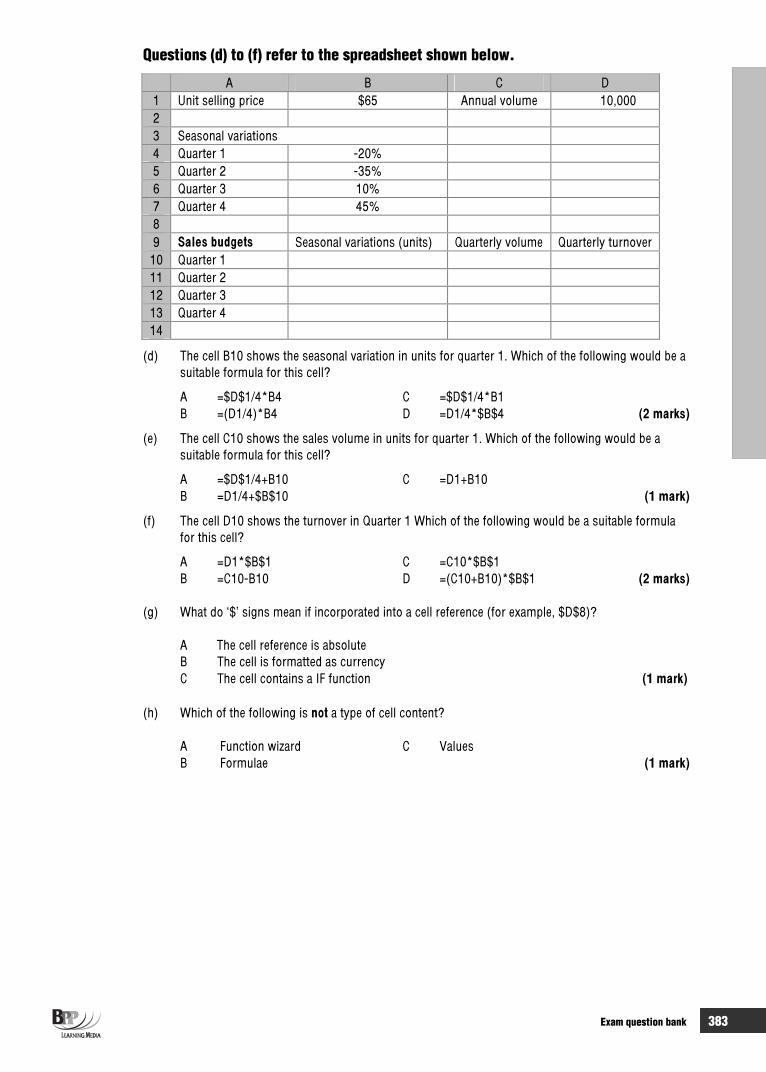
Exam question bank 383
Questions (d) to (f) refer to the spreadsheet shown below.
A B C D1 Unit selling price $65 Annual volume 10,000 23 Seasonal variations 4 Quarter 1 -20% 5 Quarter 2 -35% 6 Quarter 3 10% 7 Quarter 4 45% 89 Sales budgets Seasonal variations (units) Quarterly volume Quarterly turnover 10 Quarter 1 11 Quarter 2 12 Quarter 3 13 Quarter 4 14
(d) The cell B10 shows the seasonal variation in units for quarter 1. Which of the following would be a suitable formula for this cell?
A =$D$1/4*B4 C =$D$1/4*B1 B =(D1/4)*B4 D =D1/4*$B$4 (2 marks)
(e) The cell C10 shows the sales volume in units for quarter 1. Which of the following would be a suitable formula for this cell?
A =$D$1/4+B10 C =D1+B10 B =D1/4+$B$10 (1 mark)
(f) The cell D10 shows the turnover in Quarter 1 Which of the following would be a suitable formula for this cell?
A =D1*$B$1 C =C10*$B$1 B =C10-B10 D =(C10+B10)*$B$1 (2 marks)
(g) What do ‘$’ signs mean if incorporated into a cell reference (for example, $D$8)?
A The cell reference is absolute B The cell is formatted as currency C The cell contains a IF function (1 mark)
(h) Which of the following is not a type of cell content?
A Function wizard C Values B Formulae (1 mark)
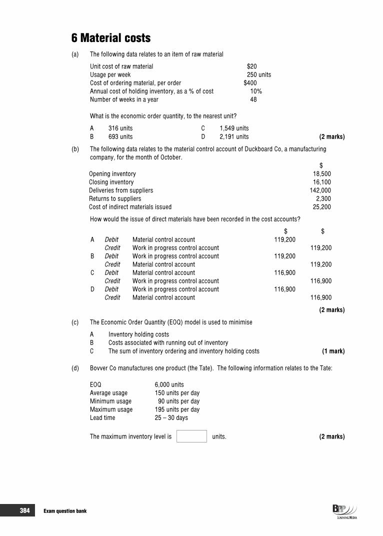
384 Exam question bank
6 Material costs (a) The following data relates to an item of raw material
Unit cost of raw material $20Usage per week 250 units Cost of ordering material, per order $400Annual cost of holding inventory, as a % of cost 10%Number of weeks in a year 48
What is the economic order quantity, to the nearest unit?
A 316 units C 1,549 units B 693 units D 2,191 units (2 marks)
(b) The following data relates to the material control account of Duckboard Co, a manufacturing company, for the month of October.
$Opening inventory 18,500Closing inventory 16,100Deliveries from suppliers 142,000Returns to suppliers 2,300Cost of indirect materials issued 25,200
How would the issue of direct materials have been recorded in the cost accounts?
$ $ A Debit Material control account 119,200
Credit Work in progress control account 119,200 B Debit Work in progress control account 119,200
Credit Material control account 119,200 C Debit Material control account 116,900
Credit Work in progress control account 116,900 D Debit Work in progress control account 116,900
Credit Material control account 116,900
(2 marks)
(c) The Economic Order Quantity (EOQ) model is used to minimise
A Inventory holding costs B Costs associated with running out of inventory C The sum of inventory ordering and inventory holding costs (1 mark)
(d) Bovver Co manufactures one product (the Tate). The following information relates to the Tate:
EOQ 6,000 units Average usage 150 units per day Minimum usage 90 units per day Maximum usage 195 units per day Lead time 25 – 30 days
The maximum inventory level is units. (2 marks)

Exam question bank 385
7 Labour costs (a) Gross wages incurred in department 1 in June were $54,000. The wages analysis shows the
following summary breakdown of the gross pay. Paid to Paid to
direct labour indirect labour$ $
Ordinary time 25,185 11,900Overtime: basic pay 5,440 3,500 premium 1,360 875Shift allowance 2,700 1,360Sick pay 1,380 300
36,065 17,935
What is the direct wages cost for department 1 in June?
A $25,185 C $34,685 B $30,625 D $36,065 (2 marks)
(b) The wages control account for A Co for February is shown below.
WAGES CONTROL ACCOUNT $ $
Bank 128,400 Work in progress control 79,400Balance c/d 12,000 Production overhead control 61,000
140,400 140,400Balance b/d 12,000
Which of the following statements about wages for February is not correct?
A Wages paid during February amounted to $128,400 B Wages for February were prepaid by $12,000 C Direct wages cost incurred during February amounted to $79,400 D Indirect wages cost incurred during February amounted to $61,000 (2 marks)
The following information relates to questions (c) and (d).
Slocombe Co budgeted to produce 10,000 units of its product (the Brahms) in the budgeted time of 50,000 hours. During the period the company produced 12,500 units in a total time of 68,750 hours.
(c) The capacity ratio for the period was % (work to one decimal place).
(2 marks)
(d) The production volume ratio for the period was % (work to one decimal place).
(2 marks)
(e) A company had 500 workers at the beginning of a period. During the period, 70 workers left the company for various reasons and 46 new workers were employed.
What is the labour turnover rate for the period (to the nearest %)?
The labour turnover rate for the period is % (2 marks)

386 Exam question bank
8 Overheads and absorption costing A company absorbs overheads based on labour hours. Data for the latest period are as follows.
Budgeted labour hours 8,500Budgeted overheads $148,750Actual labour hours 7,928Actual overheads $146,200
(a) Based on the data given above, what is the labour hour overhead absorption rate?
A $17.20 per hour C $18.44 per hour B $17.50 per hour D $18.76 per hour (2 marks)
(b) Based on the data given above, what is the amount of under-/over-absorbed overhead?
A $2,550 under-absorbed overhead C $7,460 over-absorbed overhead B $2,550 over-absorbed overhead D $7,460 under-absorbed overhead (2 marks)
(c) The budgeted production overheads and other budget data of Eiffel Co are as follows.
ProductionBudget dept XOverhead cost $36,000Direct materials cost $32,000Direct labour cost $40,000Machine hours 10,000Direct labour hours 18,000
What would be the absorption rate for Department X using the various bases of apportionment?
(a) % of direct material cost =
(b) % of direct labour cost =
(c) % of total direct cost =
(d) Rate per machine hour =
(e) Rate per direct labour hour = (2 marks)
9 Marginal and absorption costing (a) The overhead absorption rate for product Y is $2.50 per direct labour hour. Each unit of Y requires
3 direct labour hours. Inventory of product Y at the beginning of the month was 200 units and at the end of the month was 250 units. What is the difference in the profits reported for the month using absorption costing compared with marginal costing?
A The absorption costing profit would be $375 less B The absorption costing profit would be $125 greater C The absorption costing profit would be $375 greater D The absorption costing profit would be $1,875 greater (2 marks)
(b) B Co makes a product which has a variable production cost of $21 per unit and a sales price of $39 per unit. At the beginning of 20X5, there was no opening inventory and sales during the year were 50,000 units. Fixed costs (production, administration, sales and distribution) totalled $328,000. Production was 70,000 units.
The contribution per unit is $ . (2 marks)
(c) Davy Crockett Co makes hats, mainly for fancy dress costumes. The company expected to produce 25,000 hats during the year which would be expected to incur $125,000 in fixed costs. The total cost of each hat is $30 (including fixed costs) and the company can sell them for $40 each. Sales

Exam question bank 387
during the year were 15,000 hats from a production volume of 20,000. Actual fixed costs were $80,000 and there was no opening inventory.
What is the marginal costing net profit for the year? $ (2 marks)
(d) A company does not hold any opening or closing inventories.
Which of the following statements is true?
A Profits will be higher if absorption costing is used B Profits will be the same if either absorption costing or marginal costing were used C Profits will be higher if marginal costing is used (1 mark)
(e) In a marginal costing system, the formula ‘Sales – Variable Costs’ is used to calculate
A Net profit C Gross profit B Contribution (1 mark)
10 Process costing (a) A chemical is manufactured in two processes, X and Y. Data for process Y for last month are as
follows.
Material transferred from process X 2,000 litres @ $4 per litre Conversion costs incurred $12,240Output transferred to finished goods 1,600 litres
No losses occur in the process.
Closing work in progress is fully complete for material, but is only 50 per cent processed.
What is the value of the closing work in progress (to the nearest $)?
A $1,360 C $2,960 B $2,160 D $4,320 (2 marks)
(b) 20,000 litres of liquid were put into a process at the beginning of the month at a cost of $4,400. The output of finished product was 17,000 litres. The normal level of waste in this process is 20% and the waste which is identified at the end of the process can be sold at $0.50 per litre. Use this information to complete the process account below.
PROCESS ACCOUNT
Litres $ Litres $ Materials Normal waste Abnormal gains Finished goods
(2 marks)
(c) A food manufacturing process has a normal wastage of 10% of input. In a period, 3,000 kg of material was input and there was an abnormal loss of 75 kg. No inventories are held at the beginning or end of the process.
The quantity of good production achieved was kg. (2 marks)
(d) A company makes a product, which passes through a single process.
Details of the process for the last period are as follows.
Materials 5,000 kg at 50c per kg Labour $700 Production overheads 200% of labour
Normal losses are 10% of input in the process, and without further processing any losses can be sold as scrap for 20c per kg.
The output for the period was 4,200 kg from the process.

388 Exam question bank
There was no work in progress at the beginning or end of the period.
The value of the abnormal loss for the period is $ (2 marks)
(e) In a process account, abnormal losses are valued
A At good production cost less scrap value B At their scrap value C The same as good production (1 mark)
11 Joint products and by-products (a) SH Co manufactures three joint products and one by-product from a single process.
Data for May are as follows.
Opening and closing inventories NilRaw materials input $90,000Conversion costs $70,000
Output Units Sales price
$ per unit Joint product J 2,500 36 K 3,500 40 L 2,000 35 By-product M 4,000 1
By-product sales revenue is credited to the process account. Joint costs are apportioned on a physical units basis.
What were the full production costs of product K in May?
A $45,500 C $68,250 B $46,667 D $70,000 (2 marks)
(b) Samakand Preparations Co operates a continuous process producing three products and one by-product. Output from the process for one month was as follows.
Selling price per unit
Output
Joint product $ UnitsA 38 20,000B 54 40,000C 40 35,000By-productD 4 20,000
Total output costs were $4,040,000.
The saleable value of the by-product is deducted from process costs before apportioning costs to each joint product. Using the sales revenue basis for allocating joint costs, the unit valuation for joint product B was (to 2 decimal places):
A $49.50 C $50.00 B $45.00 D $100.00 (2 marks)

Exam question bank 389
(c) Robbie Co manufactures three products in a common process. Details of production and sales for a period are as follows:
Product Production Sales Selling price per unit (units) (units) $
Gary 20,000 18,000 50 Howard 15,000 10,000 40 Jason 10,000 6,000 90
Common costs for the period are $1,500,000.
Using the sales value method, what is the profit earned by product Howard during the period, assuming that no other costs are incurred in production?
Profit for product Howard is $ (2 marks)
12 Job, batch and service costing (a) Which of the following would be appropriate cost units for a transport business?
(i) Cost per tonne-kilometre (ii) Fixed cost per kilometre (iii) Maintenance cost of each vehicle per kilometre
A (i) only C (i) and (iii) only B (i) and (ii) only D All of them (2 marks)
(b) In which of the following situation(s) will job costing normally be used?
Production is continuous
Production of the product can be completed in a single accounting period
Production relates to a single special order (1 mark)
(c) Consider the following features and identify whether they relate to job costing, contract costing, service costing or none of these costing methods.
J = Job costing C = Contract costing S = Service costing N = None of these costing methods
(i) Production is carried out in accordance with the wishes of the customer
(ii) Work is usually of a relatively long duration
(iii) Work is usually undertaken on the contractor's premises
(iv) Costs are averaged over the units produced in the period
(v) It establishes the costs of services rendered
(2 marks)

390 Exam question bank
(d) Ali Pali Co is a small jobbing company. Budgeted direct labour hours for the current year were 45,000 hours and budgeted direct wages costs were $180,000.
Job number 34679, a rush job for which overtime had to be worked by skilled employees, had the following production costs.
$ $Direct materials 2,000Direct wages Normal rate (400 hrs) 2,000 Overtime premium 500
2,500Production overhead 4,000
8,500Production overhead is based on a direct labour hour rate
If production overhead had been based on a percentage of direct wages costs instead, the production cost of job number 34679 would have been:
A $5,500 C $10,250 B $9,000 D $10,750 (2 marks)
13 Budgeting (a) What does the statement 'sales is the principal budget factor' mean?
A The level of sales will determine the level of cash at the end of the period B The level of sales will determine the level of profit at the end of the period C The company's activities are limited by the level of sales it can achieve (1 mark)
(b) When preparing a production budget, the quantity to be produced equals
A sales quantity + opening inventory of finished goods + closing inventory of finished goods B sales quantity – opening inventory of finished goods + closing inventory of finished goods C sales quantity – opening inventory of finished goods – closing inventory of finished goods D sales quantity + opening inventory of finished goods – closing inventory of finished goods
(2 marks)
(c) PQ Co plans to sell 24,000 units of product R next year. Opening inventory of R is expected to be 2,000 units and PQ Co plans to increase inventory by 25 per cent by the end of the year. How many units of product R should be produced next year?
A 23,500 units C 24,500 units B 24,000 units D 30,000 units (2 marks)
(d) Each unit of product Alpha requires 3 kg of raw material. Next month's production budget for product Alpha is as follows.
Opening inventories:
Raw materials 15,000 kg Finished units of Alpha 2,000 units Budgeted sales of Alpha 60,000 units
Planned closing inventories:
Raw materials 7,000 kg Finished units of Alpha 3,000 units
The number of kilograms of raw materials that should be purchased next month is:
A 172,000 C 183,000 B 175,000 D 191,000 (2 marks)

Exam question bank 391
(e) Budgeted sales of X for December are 18,000 units. At the end of the production process for X, 10% of production units are scrapped as defective. Opening inventories of X for December are budgeted to be 15,000 units and closing inventories will be 11,400 units. All inventories of finished goods must have successfully passed the quality control check. The production budget for X for December, in units is
A 12,960 C 15,840 B 14,400 D 16,000 (2 marks)
(f) In a situation where there are no production resource limitations, which of the following must be available for the material usage budget to be completed? Tick all that apply.
(a) Production volume from the production budget
(b) Budgeted change in materials inventory
(c) Standard material usage per unit (2 marks)
(g) If a company has no production resource limitations, in which order would the following budgets be prepared?
Order
Material usage budget
Sales budget
Material purchase budget
Finished goods inventory budget
Production budget
Material inventory budget
(2 marks)
(h) True False (a) Budgetary control procedures are useful only to maintain
control over an organisation's expenditure
(b) A prerequisite of flexible budgeting is a knowledge of cost behaviour patterns
(c) Fixed budgets are not useful for control purposes
(2 marks)
14 Standard costing (a) Which of the following would not be used to estimate standard direct material prices?
A The availability of bulk purchase discounts B Purchase contracts already agreed C The forecast movement of prices in the market D Performance standards in operation (2 marks)
(b) JC Co operates a bottling plant. The liquid content of a filled bottle of product T is 2 litres. During the filling process there is a 30% loss of liquid input due to spillage and evaporation. The standard price of the liquid is $1.20 per litre. The standard cost of the liquid per bottle of product T, to the nearest cent, is
A $2.40 C $3.12 B $2.86 D $3.43 (2 marks)

392 Exam question bank
(c) Standard costing provides which of the following? Tick all that apply.
(a) Targets and measures of performance
(b) Information for budgeting
(c) Simplification of inventory control systems
(d) Actual future costs (2 marks)
(d) Calculate the standard cost of producing 100 wheels for a toy car using the information given below. Fill in the shaded box.
Bending Cutting Assembly Standard labour rates of pay per hour $ 4 6 5Standard labour rates per 100 wheels (hours) 0.8 0.5 1.2
STANDARD COST CARD
Toy car wheels Part number 5917B - 100 wheels Date: Quantity Rate/price Total
$Direct materials Tyres 100 10c eachSteel strip 50 $10.40 per 100 Wire 1000 2c each Direct labour hours $ BendingCutting Assembly
STANDARD COST
(2 marks)
(e) What is an attainable standard?
A A standard that can be attained under perfect operating conditions, and which does not include an allowance for wastage, spoilage, machine breakdowns and other inefficiencies
B A standard that is based on currently attainable working conditions C A standard that can be attained if production is carried out efficiently, machines are
operated properly and/or materials are used properly, with some allowance being made for waste and inefficiencies (1 mark)

Exam question bank 393
15 Basic variance analysis (a) The standard cost information for SC's single product shows the standard direct material content
to be 4 litres at $3 per litre.
Actual results for May were:
Production 1,270 units Material used 5,000 litres at a cost of $16,000
All of the materials were purchased and used during the period. The direct material price and usage variances for May are:
Material price Material usage
A $1,000 (F) $240 (F) B $1,000 (A) $240 (F) C $1,000 (F) $240 (A) D $1,000 (A) $256 (F) (2 marks)
The following information relates to questions (b) and (c) The standard variable production overhead cost of product B is as follows.
4 hours at $1.70 per hour = $6.80 per unit
During period 3 the production of B amounted to 400 units. The labour force worked 1,690 hours, of which 30 hours were recorded as idle time. The variable overhead cost incurred was $2,950.
(b) The variable production overhead expenditure variance for period 3 was
A $77 adverse C $128 favourable B $128 adverse D $230 adverse (2 marks)
(c) The variable production overhead efficiency variance for period 3 was
A $102 favourable C $105 adverse B $102 adverse D $153 adverse (2 marks)
(d) Which of the following would help to explain a favourable direct material price variance?
Would help Would not helpto explain to explainvariance variance
(a) The standard price per unit of direct material was unrealistically high
(b) Output quantity was greater than budgeted and it was possible to obtain bulk purchase discounts
(c) The material purchased was of a higher quality than standard
(2 marks)

394 Exam question bank
16 Further variance analysis(a) W Co uses a standard absorption costing system. The following data relates to one of its products.
$ per unit $ per unitSelling price 27.00Variable costs 12.00Fixed costs 9.00
21.00Profit 6.00
Budgeted sales for control period 7 were 2,400 units, but actual sales were 2,550 units. The revenue earned from these sales was $67,320.
Profit reconciliation statements are drawn up using absorption costing principles. What sales variances would be included in such a statement for period 7?
Price Volume A $1,530 (F) $900 (F) B $1,530 (A) $900 (F) C $1,530 (F) $900 (A) D $1,530 (A) $900 (A) (2 marks)
(b) A standard marginal costing system:
(i) calculates fixed overhead variances using the budgeted absorption rate per unit (ii) calculates sales volume variances using the standard contribution per unit (iii) values finished goods stock at the standard variable cost of production
Which of the above statements is/are correct?
A (i), (ii) and (iii) C (ii) and (iii) only B (i) and (ii) only D (i) and (iii) only (2 marks)
(c) Diddly Co earned a profit of $305,000 in the last month. Variances were as follows.
Labour: Rate 15,250 (F) Efficiency 10,750 (A)
Material: Usage 8,675 (A) Price 9,825 (F)
Variable overheads Efficiency 6,275 (A) Expenditure 2,850 (F)
Fixed overheads: Expenditure 7,000 (F)
Sales: Price 25,000 (A) Volume 32,000 (F)
What was Diddly Co’s budgeted profit for last month?
A $321,225 C $371,925 B $288,775 D $254,300 (2 marks)

Exam question bank 395
17 Cost-volume-profit analysis (a) A company manufactures a single product for which cost and selling price data are as follows.
Selling price per unit $12 Fixed costs per month $96,000 Variable cost per unit $8 Budgeted monthly sales 30,000 units
The margin of safety, expressed as a percentage of budgeted monthly sales, is (to the nearest whole number):
A 20% C 73% B 25% D 125% (2 marks)
(b)
In the above breakeven chart, the contribution at level of activity x can be read as:
A distance A C distance C B distance B D distance D (2 marks)
(c) A company manufactures a single product with a selling price of $100 per unit. Cost information is as follows:
$Material cost per unit 45 Labour cost per unit 14 Variable overheads per unit 10
What is the breakeven sales revenue for a period if the fixed costs for that period are $450,000?
The breakeven sales revenue is $ (2 marks)
(d) S Co manufactures a single product, V. Data for the product are as follows.
$ per unitSelling price 40Direct material cost 8Direct labour cost 6Variable production overhead cost 4Variable selling overhead cost 2Fixed overhead cost 10Profit per unit 10
The contribution/volume ratio for product V is (2 marks)

396 Exam question bank
(e) Fast Fandango Co manufactures a single product, the FF, which sells for $10. At 75% capacity, which is the normal level of activity for the factory, sales are $600,000 per period.
The cost of these sales are as follows.
Direct cost per unit $3Production overhead $156,000 (including variable costs of $30,000) Sales costs $ 80,000Distribution costs $ 60,000 (including variable costs of $15,000) Administration overhead $ 40,000 (including variable costs of $9,000)
The sales costs are fixed with the exception of sales commission which is 5% of sales value.
(a) The contribution per unit of product FF is $ (2 marks)
(b) The fixed cost per period is $ (2 marks)
(c) The breakeven volume of sales per period is units (2 marks)
18 Relevant costing and decision-making (a) Sue is considering starting a new business and she has already spent $5,000 on market research
and intends to spend a further $2,000.
In the assessment of the relevant costs of the decision to set up the business, market research costs are:
A a sunk cost of $7,000 B a sunk cost of $5,000 and an incremental cost of $2,000 C a sunk cost of $2,000 and an incremental cost of $5,000 D an opportunity cost of $7,000 (2 marks)
(b) ABC Co is in the process of deciding whether or not to accept a special order. The order will require 100 litres of liquid X. ABC Ltd has 85 litres of liquid X in inventory but no longer produces the product which required liquid X. It could therefore sell the 85 litres for $2 per litre if it rejected the special order. The liquid was purchased three years ago at a price of $8 per litre but its replacement cost is $10 per litre. What is the relevant cost of liquid X to include in the decision-making process?
A $200 C $800 B $320 D $1,000 (2 marks)
(c) V Co manufactures three products which have the following selling prices and costs per unit.
V1 V2 V3 $ $ $ Selling price 30.00 36.00 34.00Costs per unit Direct materials 8.00 10.00 20.00 Direct labour 4.00 8.00 3.60OverheadVariable 2.00 4.00 1.80 Fixed 9.00 6.00 2.70
23.00 28.00 28.10
Profit per unit 7.00 8.00 5.90
All three products use the same type of labour.

Exam question bank 397
In a period in which labour is in short supply, the rank order of production is:
V1 …………………………
V2 …………………………
V3 …………………………
(d) A company manufactures four products. Details of each product are as follows:
W X Y Z$ $ $ $
Selling price 80 65 85 90 Costs per unit Direct labour 30 15 25 30 Direct materials 15 20 20 25 Variable overheads 5 7.50 12.50 15Fixed overheads 20 15 10 15 Profit per unit 10 7.50 7.50 5
Labour is charged to products at a rate of $5 per hour.
If labour is in short supply in the next period, the company should maximise production of:
A Product W C Product Y B Product X D Product Z (2 marks)
(e) Chloe Co purchased machinery for $300,000 five years ago and is now considering whether it would be worthwhile replacing it/
The current replacement cost of the machinery is $525,000 and scrap value of the existing machine is $375,000. However the machine could still be used by Chloe Co and would generate income of $450,000.
The relevant cost of the machine is $ (2 marks)
19 Linear programming (a) A company produces two types of orange juice, ordinary (X cartons per year) and premium (Y
cartons per year). Which of the following inequalities represents the fact that the amount of ordinary orange juice produced must be no more than twice the amount of premium orange juice produced.
A X 2Y C 2X Y B 2X Y D X 2Y (2 marks)
(b) In a linear programming problem, the constraints are X 41 and Y 19. Describe the feasible region, assuming where appropriate that the axes also constitute boundaries.
A A rectangle to the left of X = 41 and below Y = 19 B An infinite rectangle to the right of X = 41 and below Y = 19 C An infinite region above Y = 19 and to the right of X = 41 D An infinite rectangle to the left of X = 41 and above Y = 19 (2 marks)
(2 marks)

398 Exam question bank
(c) A company manufactures two products – B and C – with details as follows: B C
Labour hours per unit 4 5 Material (kg) per unit 4 9
There are 12,000 labour hours and 18,000 kg of material available during a period and the company has determined that the optimal production can be found at the intersection of the labour and material constraints.
How many units of each product should be produced at the optimal point?
The company should produce units of B and units of C. (2 marks)

Exam answer bank 399
ANSWERS
1 Information for management (a) D Data is the raw material for data processing. Information is data that has been processed in
such a way as to be meaningful to the person who receives it. Statement I is therefore incorrect.
An organisation's financial accounting records are an example of an internal source of information. Statement II is therefore incorrect.
The main objective of a non-profit making organisation is usually to provide goods and services. Statement III is therefore correct.
(b) A Financial accounts (not management accounts) detail the performance of an organisation over a defined period and the state of affairs at the end of that period. Managementaccounts are used to aid management record, plan and control the organisation's activities and to help the decision-making process.
(c) C Higher level management are likely to be involved with taking decisions at all levels within an organisation.
(d) D Cost accounting can also be used to provide inventory valuations for external reporting.
(e) C Obtaining data about actual results is part of the control process.
2 Cost classification (a) D It would be appropriate to use the cost per invoice processed and the cost per supplier
account for control purposes. Therefore items (ii) and (iii) are suitable cost units and the correct answer is D.
Postage cost, item (i), is an expense of the department, therefore option A is not a suitable cost unit.
If you selected option B or option C you were probably rushing ahead and not taking care to read all the options. Items (ii) and (iii) are suitable cost units, but neither of them are the only suitable suggestions.
(b) A Special designs, and the hire of tools etc for a particular job can be traced to a specific cost unit. Therefore they are direct expenses and the correct answer is A.
Item (iii) is a selling and distribution overhead and item (iv) describes production overheads.
Appropriate Not appropriate (c) (a) Vehicle cost per passenger -
kilometre
(b) Fuel cost for each vehicle per kilometre
(c) Fixed cost per kilometre
(d) B A direct cost is one that can be directly related to a unit of output; an unavoidable cost is one that would be incurred whether or not a certain activity took place.
(e) B The cost per hour of operating a machine is an example of the cost of input resource, which might form part of the total cost of a cost unit.
A measure of output of work in a standard hour is an indication of productivity.

400 Exam answer bank
3 Cost behaviour (a) A Variable costs are conventionally deemed to increase or decrease in direct proportion to
changes in output. Therefore the correct answer is A. Description B implies a changing unit rate, which does not comply with this convention. Description C relates to a fixed cost.
(b) B The cost depicted begins as a linear variable cost, increasing at a constant rate in line with activity. At a certain point the cost becomes fixed regardless of the level of activity. The vehicle hire costs follow this pattern.
Graphs for the other options would look like this.
Totalcost
Level of activity
TotalCost
Totalcost
Level of activity
Option D
Option COption A
(c) (a) FIXED COST
(b) VARIABLE COST
(c) STEPPED FIXED COST
(d) SEMI-VARIABLE COST
(d) D Bob cannot control the rent within the six-month period as he is unable to get out of the agreement during this time, therefore the rent is an uncontrollable cost.
Rent is not a fixed cost as the landlord may change it during the period.
Bob has agreed to pay the rent therefore he cannot avoid it (that is, rent is not an unavoidable cost).
A semi-variable cost comprises a fixed and a variable element, which is not the case with Bob Co’s rent.
(e) The total cost for period 3 if 15,500 square metres are decorated is $58,250
The first step is to eliminate the extra fixed costs from period 2 total costs so that we are comparing ‘like with like’.
Total costs with no extra fixed costs = $56,000 - $6,000 = $50,000
We can now use the high-low method in the usual way to calculate variable cost per unit.
$ $
$

Exam answer bank 401
Square metres $High output 14,000 Total cost 50,000Low output 10,000 Total cost 44,000
4,000 6,000
Variable cost per square metre = $6,000/4,000 = $1.50
Using the high level to calculate fixed costs: $
Total costs 56,000 (includes the step up in fixed costs)Total variable costs 21,000 (14,000 square metres x $1.50 per square metre)Total fixed costs 35,000
Total cost for 15,500 square metres: $
Total variable costs 23,250 (15,500 square metres x $1.50)Total fixed costs 35,000 (see above)Total costs 58,250
4 Correlation and regression (a) D If C = 1,000 + 250P, then fixed costs are $1,000 and variable costs are $250 per unit.
(b) D The correlation coefficient of 0.9 is very close to 1 and so there is a very strong relationship between x and y.
(c) B It does not matter what the sign of the correlation coefficient is – the size of the correlation coefficient between C and D (0.7) is larger than that between A and B (0.4) therefore the relationship between C and D is stronger than between A and B.
(d) The expected profit for next month is calculated as:
($500,000 3) ($800,000 1)
(3 1) = $575,000
(e) The expected contribution for the period is $12,460.
Expected sales demand
(0.4 4,000 units) + (0.5 4,500 units) + (0.1 6,000 units ) = 4,450 units
Expected variable cost per unit
(0.2 $5.50) + (0.5 $6.00) + (0.3 $7.00) = $6.20 per unit
Expected contribution $
Expected sales revenue (4,450 $9) 40,050Expected variable costs (4,450 $6.20) 27,590Expected contribution 12,460
5 Spreadsheets (a) B A line graph is the best way of illustrating a trend over time.
(b) B A macro is used for automating frequently repeated tasks
(c) D II only
Relative cell references (B3) change when you copy formulae to other locations. Absolute cell references ($B$3) stay the same when you copy formulae to other locations.

402 Exam answer bank
(d) A =$D$1/4*B4
This formula will divide the annual turnover by 4 and multiply the result by the seasonal variation. The $ signs show that the cell reference for D1 is absolute so the reference will stay the same when the formula is copied into the cells below.
(e) A =$D$1/4+B10
This formula will divide the annual turnover by 4 and add the result to the seasonal variation found in cell B10. The $ signs show that the cell reference for D1 is absolute so the reference will stay the same when the formula is copied into the cells below.
(f) C =C10*$B$1
This formula will multiply the quarterly volume in units from cell C10 by the unit selling price in cell B1. The $ signs show that the cell reference for B1 is absolute so the reference will stay the same when the formula is copied into the cells below
(g) A The cell reference is absolute.
(h) A A wizard is a tool available to help with or shorten tasks.
6 Material costs
(a) D EOQ = 10%$20
48)(250$4002 = 2,191
Therefore the correct answer is D.
If you selected option A you used weekly usage in the calculations instead of the annual usage.
If you selected option B you did not take ten per cent of the material cost as the annual inventory holding cost.
If you selected option C you omitted the 2.
(b) D The easiest way to solve this question is to draw up a stores ledger control account.
STORES LEDGER CONTROL ACCOUNT
$ $Opening stock b/f 18,500 Payables (returns) 2,300Payables/cash (deliveries) 142,000 Overhead account (indirect
materials) 25,200WIP (balancing figure) 116,900Closing inventory c/f 16,100
160,500 160,500
If you selected option C you determined the correct value of the direct materials issued but you reversed the entries.
If you selected options A or B you placed the figure for returns on the wrong side of your account, and in option A you reversed the entries for the issue of direct materials from stores.
(c) C There is a trade off between inventory ordering and inventory holding costs. If we assume that the cost of purchasing an item of inventory remains constant, the EOQ formula calculates the order size at which the total of these two costs is minimised.
(d) The maximum inventory level is 9,600 units.
Reorder level = maximum usage x maximum lead time
= 195 x 30 = 5,850 units

Exam answer bank 403
Maximum inventory level = reorder level + reorder quantity – (minimum usage x minimum lead time)
= 5,850 + 6,000 – (90 x 25)
= 9,600 units
7 Labour costs (a) B The only direct costs are the wages paid to direct workers for ordinary time, plus the basic
pay for overtime.
$25,185 + $5,440 = $30,625.
If you selected option A you forgot to include the basic pay for overtime of direct workers, which is always classified as a direct labour cost.
If you selected option C you have included overtime premium and shift allowances, which are usually treated as indirect costs. However, if overtime and shiftwork are incurred specifically for a particular cost unit, then they are classified as direct costs of that cost unit. There is no mention of such a situation here.
Option D includes sick pay, which is classified as an indirect labour cost.
(b) B The credit balance on the wages control account indicates that the amount of wages incurred and analysed between direct wages and indirect wages was higher than the wages paid through the bank. Therefore there was a $12,000 balance of wages owing at the end of February and statement B is not correct. Therefore the correct option is B.
Statement A is correct. $128,400 of wages was paid from the bank account.
Statement C is correct. $79,400 of direct wages was transferred to the work in progress control account.
Statement D is correct. $61,000 of indirect wages was transferred to the production overhead control account.
(c) The capacity ratio for the period was 137.5 %
Labour capacity ratio = budgeted Hours
workedhoursActual x 100% = (68,750/50,000) x 100% = 137.5%
(d) The production volume ratio for the period was 125 %
Production volume ratio = budgeted Hours
hours standard or expected in measured Output
= 12,500 × 5 hours
50,000 100%
= 125%
[Expected hours per unit = budgeted hours (50,000 units) / budgeted output (10,000)]
(e) The labour turnover rate for the period is 9%.
Labour turnover rate = period in employees of number Average
tsReplacemen x 100%
Average number of employees = (500 +[500 – 70 + 46])/2 = 488
Labour turnover rate = (46/488) 100% = 9%

404 Exam answer bank
8 Overheads and absorption costing
(a) B Overhead absorption rate =hours labour budgeted
overheads budgeted=
500,8750,148$
= $17.50 per hr
If you selected option A you divided the actual overheads by the budgeted labour hours. Option C is based on the actual overheads and actual labour hours. If you selected option D you divided the budgeted overheads by the actual hours.
(b) D $Overhead absorbed = $17.50 7,928 = 138,740Overhead incurred = 146,200Under-absorbed overhead = 7,460
If you selected options A or B you calculated the difference between the budgeted and actual overheads and interpreted it as an under or over absorption. If you selected option C you performed the calculations correctly but misinterpreted the result as an over absorption.
(c) (a) % of direct material cost = 112.5%
(b) % of direct labour cost = 90%
(c) % of total direct cost = 50%
(d) Rate per machine hour = $3.60
(e) Rate per direct labour hour = $2
Workings
(a) % of direct materials cost $32,000$36,000
100% = 112.5%
(b) % of direct labour cost $40,000$36,000
100% = 90%
(c) % of total direct cost $72,000$36,000
100% = 50%
(d) Rate per machine hour hrs10,000
$36,000 = $3.60 per machine hour
(e) Rate per direct labour hour hrs18,000
$36,000 = $2 per direct labour hour
9 Marginal and absorption costing (a) C Difference in profit = change in inventory level fixed overhead per unit
= (200 – 250) ($2.50 3) = $375
The absorption costing profit will be greater because inventories have increased.
If you selected option A you calculated the correct profit difference but the absorption costing profit would be greater because fixed overheads are carried forward in the increasing inventory levels.
If you selected option B you multiplied the inventory difference by the direct labour-hour rate instead of by the total overhead cost per unit, which takes three hours.

Exam answer bank 405
If you selected option D you based the profit difference on the closing inventory only (250 units $2.50 3).
(b) (a) The contribution per unit is $900,000/50,000 = $18
(c) $ $
Sales (at $40 per unit) 600,000Opening inventory –Variable production cost ($25 20,000) (W1) 500,000Less closing inventory ($25 5,000) 125,000Variable cost of sales 375,000Contribution 225,000Less fixed costs 80,000Profit 145,000
W1 Variable production cost per unit = Total cost per unit – fixed cost per unit
= $30 – ($125,000/25,000 units) = $25 per unit
(d) B Profits will be the same under both methods, as opening inventory equals closing inventory.
It is changes in inventory levels that cause these two costing systems to give different profit figures.
(e) B Gross profit is used in an absorption costing system; net profit = contribution – fixed costs.
10 Process costing(a) C Step 1. Determine output and closing WIP
Equivalent units of productionInput Output Total Process X Conversion costsUnits Units Units % Units %2,000 Finished units 1,600 1,600 100 1,600 100
Closing inventory (balance)
400 400 100 200 50
2,000 2,000 2,000 1,800
Step 2. Calculate cost per unit of output and WIP
Equivalent Cost perInput Cost units equivalent unit
$ $Process X material 8,000 2,000 4.00Conversion costs 12,240 1,800 6.80
10.80
Step 3. Calculate total cost of closing WIP
Using the unit rates from answer (a) step 2: Cost Number of Cost perelement equivalent units equivalent unit Total
$ $Work in progress Process X material 400 4.00 1,600
Conversion costs 200 6.80 1,360 2,960
If you selected option A you only included the conversion costs in your calculation. If you selected option B you did not account for the fact that closing WIP was fully complete for materials and multiplied total cost per equivalent unit by 200. Option D does not allow for the fact that the work in progress (WIP) is incomplete when calculating the total cost of WIP.

406 Exam answer bank
(b) PROCESS ACCOUNT
Litres $ Litres $Materials 20,000 4,400 Normal waste
(4,000 $0.50) 4,000 2,000Finished goods 17,000 2,550
Abnormal gain 1,000 15021,000 4,550 21,000 4,550
Workings
Normal loss = 20% 20,000 litres = 4,000 litres
Expected output = 20,000 – 4,000 = 16,000 litres
Cost per unit = output Expected
loss normalofproceedsscrap-costsProcess
= litres 16,000
$0.50)(4,000$4,400
= litres 16,000$2,000$4,400
= litres 16,000
$2,400
= $0.15
(c) The quantity of good production achieved was 2,625 kg.
Good production = input – normal loss – abnormal loss = 3,000 – (10% × 3,000) – 75 = 3,000 – 300 – 75 = 2,635 kg
(d) The value of the abnormal loss for the period is $ 300
kgInput 5,000Normal loss (10% 5,000 kg) (500)Abnormal loss (300)Output 4,200
Cost per kg = utputExpected o
al lossue of normscrap valts cosInput
= 500000,5
100$ *600,4$
= 500,4500,4$
= $1.00
Value of abnormal loss = 300 $1.00 = $300
$*Materials (5,000 kg 0.5) 2,500 Labour 700 Production overhead 1,400
4,600
(e) C Abnormal losses have the same value as good production.

Exam answer bank 407
11 Joint products and by-products(a) C Net process costs
$Raw materials 90,000Conversion costs 70,000Less by-product revenue (4,000)Net process costs 156,000
Apportionment of net process costs
Units Apportioned costs$ $
Product J 2,500 $156,000 (2,500/8,000) 48,750 K 3,500 $156,000 (3,500/8,000) 68,250 L 2,000 $156,000 (2,000/8,000) 39,000
8,000 156,000
If you selected option A or B you apportioned a share of the process costs to the by-product, and with option B or D you did not deduct the by-product revenue from the process costs.
(b) A WorkingsSales revenue
Joint product $A 760,000 ($38 20,000)B 2,160,000 ($54 40,000)C 1,400,000 ($40 35,000)Total sales revenues 4,320,000
Joint costs to be allocated = Total output costs – sales revenue from by-product D
= $4,040,000 – $80,000 ($4 × 20,000) = $3,960,000
Costs allocated to joint product B = $4,320,000$2,160,000
$3,960,000
= $1,980,000
Unit valuation (joint product B) = 40,000
$1,980,000
= $49.50 (to 2 decimal places)
If you selected option B, you forgot to deduct the sales revenue (from by-product D) from the joint costs to be allocated.
If you selected option C, you excluded by-product D from your calculations completely.
If you selected option D, you divided the total sales revenue (instead of the joint costs to be allocated) by the number of units of joint product D.
(c) The correct answer is $40,000.
Remember to allocate costs according to sales value of production rather than sales value of units sold.
Sales value of production: $ Gary (20,000 units x $50) 1,000,000Howard (15,000 x $40) 600,000 Jason (10,000 x $90) 900,000
2,500,000
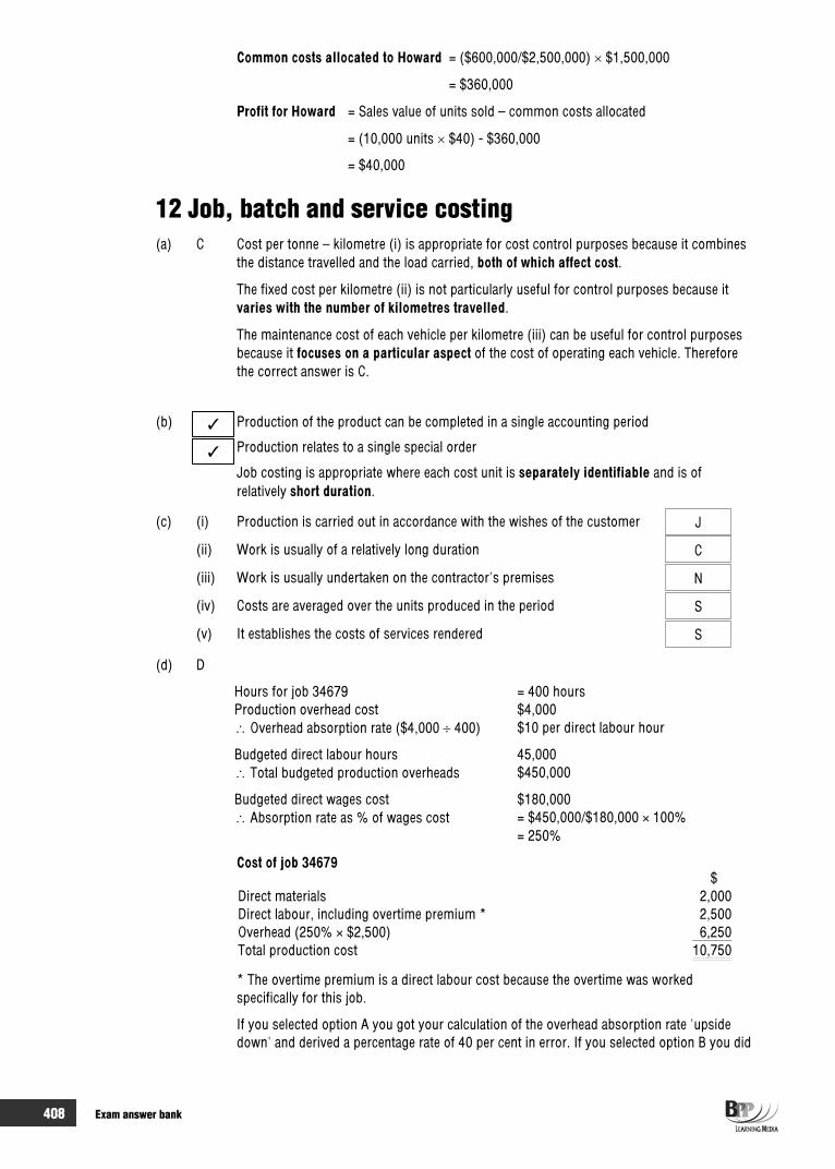
408 Exam answer bank
Common costs allocated to Howard = ($600,000/$2,500,000) $1,500,000
= $360,000
Profit for Howard = Sales value of units sold – common costs allocated
= (10,000 units $40) - $360,000
= $40,000
12 Job, batch and service costing (a) C Cost per tonne – kilometre (i) is appropriate for cost control purposes because it combines
the distance travelled and the load carried, both of which affect cost.
The fixed cost per kilometre (ii) is not particularly useful for control purposes because it varies with the number of kilometres travelled.
The maintenance cost of each vehicle per kilometre (iii) can be useful for control purposes because it focuses on a particular aspect of the cost of operating each vehicle. Therefore the correct answer is C.
(b) Production of the product can be completed in a single accounting period
Production relates to a single special order
Job costing is appropriate where each cost unit is separately identifiable and is of relatively short duration.
(c) (i) Production is carried out in accordance with the wishes of the customer J
(ii) Work is usually of a relatively long duration C
(iii) Work is usually undertaken on the contractor's premises N
(iv) Costs are averaged over the units produced in the period S
(v) It establishes the costs of services rendered S
(d) D
Hours for job 34679 = 400 hours Production overhead cost $4,000
Overhead absorption rate ($4,000 400) $10 per direct labour hour
Budgeted direct labour hours 45,000 Total budgeted production overheads $450,000
Budgeted direct wages cost $180,000 Absorption rate as % of wages cost = $450,000/$180,000 × 100%
= 250%
Cost of job 34679 $
Direct materials 2,000Direct labour, including overtime premium * 2,500Overhead (250% × $2,500) 6,250Total production cost 10,750
* The overtime premium is a direct labour cost because the overtime was worked specifically for this job.
If you selected option A you got your calculation of the overhead absorption rate 'upside down' and derived a percentage rate of 40 per cent in error. If you selected option B you did
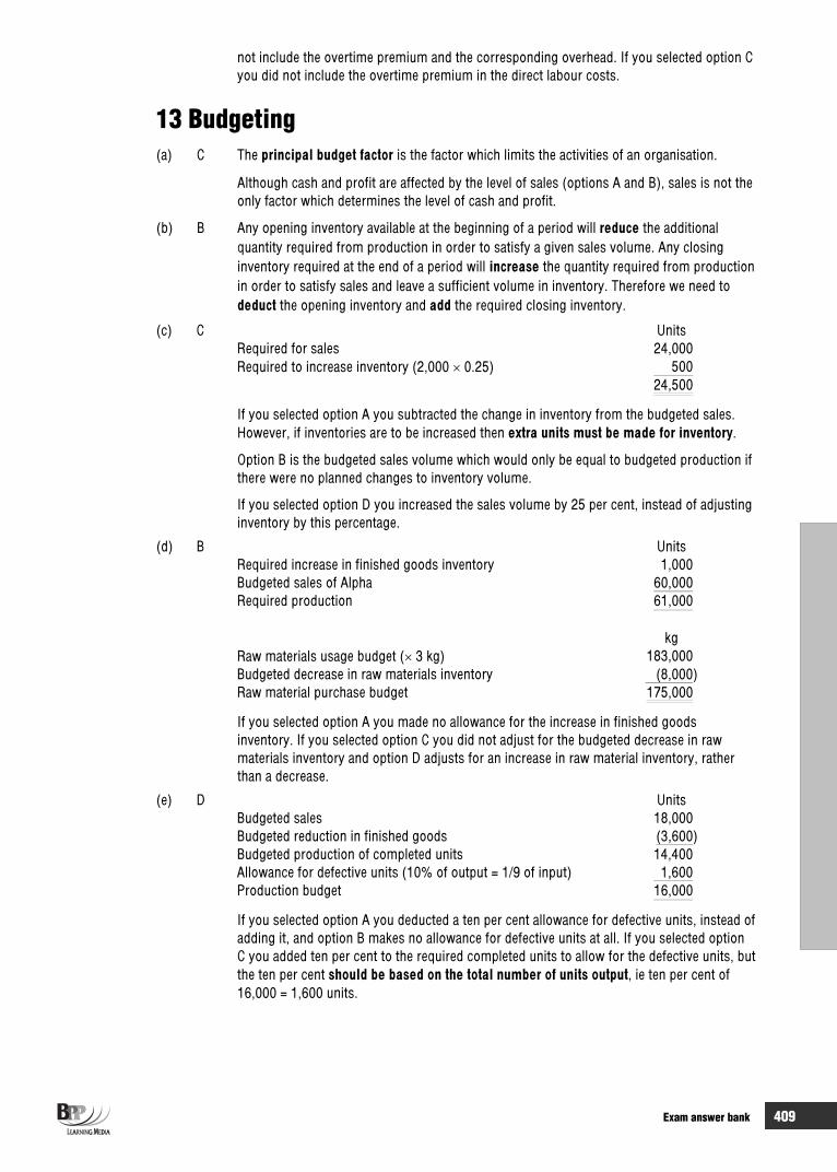
Exam answer bank 409
not include the overtime premium and the corresponding overhead. If you selected option C you did not include the overtime premium in the direct labour costs.
13 Budgeting (a) C The principal budget factor is the factor which limits the activities of an organisation.
Although cash and profit are affected by the level of sales (options A and B), sales is not the only factor which determines the level of cash and profit.
(b) B Any opening inventory available at the beginning of a period will reduce the additional quantity required from production in order to satisfy a given sales volume. Any closing inventory required at the end of a period will increase the quantity required from production in order to satisfy sales and leave a sufficient volume in inventory. Therefore we need to deduct the opening inventory and add the required closing inventory.
(c) C UnitsRequired for sales 24,000Required to increase inventory (2,000 0.25) 500
24,500
If you selected option A you subtracted the change in inventory from the budgeted sales. However, if inventories are to be increased then extra units must be made for inventory.
Option B is the budgeted sales volume which would only be equal to budgeted production if there were no planned changes to inventory volume.
If you selected option D you increased the sales volume by 25 per cent, instead of adjusting inventory by this percentage.
(d) B UnitsRequired increase in finished goods inventory 1,000Budgeted sales of Alpha 60,000Required production 61,000
kgRaw materials usage budget ( 3 kg) 183,000Budgeted decrease in raw materials inventory (8,000)Raw material purchase budget 175,000
If you selected option A you made no allowance for the increase in finished goods inventory. If you selected option C you did not adjust for the budgeted decrease in raw materials inventory and option D adjusts for an increase in raw material inventory, rather than a decrease.
(e) D UnitsBudgeted sales 18,000Budgeted reduction in finished goods (3,600)Budgeted production of completed units 14,400Allowance for defective units (10% of output = 1/9 of input) 1,600Production budget 16,000
If you selected option A you deducted a ten per cent allowance for defective units, instead of adding it, and option B makes no allowance for defective units at all. If you selected option C you added ten per cent to the required completed units to allow for the defective units, but the ten per cent should be based on the total number of units output, ie ten per cent of 16,000 = 1,600 units.
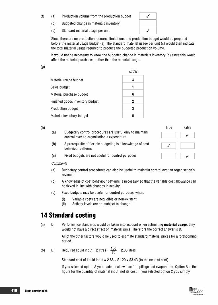
410 Exam answer bank
(f) (a) Production volume from the production budget
(b) Budgeted change in materials inventory
(c) Standard material usage per unit
Since there are no production resource limitations, the production budget would be prepared before the material usage budget (a). The standard material usage per unit (c) would then indicate the total material usage required to produce the budgeted production volume.
It would not be necessary to know the budgeted change in materials inventory (b) since this would affect the material purchases, rather than the material usage.
(g)Order
Material usage budget 4
Sales budget 1
Material purchase budget 6
Finished goods inventory budget 2
Production budget 3
Material inventory budget 5
(h) True False (a) Budgetary control procedures are useful only to maintain
control over an organisation's expenditure
(b) A prerequisite of flexible budgeting is a knowledge of cost behaviour patterns
(c) Fixed budgets are not useful for control purposes
Comments
(a) Budgetary control procedures can also be useful to maintain control over an organisation's revenue.
(b) A knowledge of cost behaviour patterns is necessary so that the variable cost allowance can be flexed in line with changes in activity.
(c) Fixed budgets may be useful for control purposes when:
(i) Variable costs are negligible or non-existent (ii) Activity levels are not subject to change
14 Standard costing (a) D Performance standards would be taken into account when estimating material usage, they
would not have a direct effect on material price. Therefore the correct answer is D.
All of the other factors would be used to estimate standard material prices for a forthcoming period.
(b) D Required liquid input = 2 litres × 70
100 = 2.86 litres
Standard cost of liquid input = 2.86 × $1.20 = $3.43 (to the nearest cent)
If you selected option A you made no allowance for spillage and evaporation. Option B is the figure for the quantity of material input, not its cost. If you selected option C you simply

Exam answer bank 411
added an extra 30 per cent to the finished volume. However, the wastage is 30 per cent of the liquid input, not 30 per cent of output.
(c) (a) Targets and measures of performance
(b) Information for budgeting
(c) Simplification of inventory control systems
(d) Actual future costs
Standard costing provides targets for achievement, and yardsticks against which actual performance can be monitored (item (a)). It also provides the unit cost information forevaluating the volume figures contained in a budget (item (b)). Inventory control systems are simplified with standard costing. Once the variances have been eliminated, all inventory units are evaluated at standard price (item (c)).
Item (d) is incorrect because standard costs are an estimate of what will happen in the future, and a unit cost target that the organisation is aiming to achieve.
(d)
STANDARD COST CARD
Toy car wheels Part number 5917B - 100 wheels Date: Quantity Rate/price Total
$Direct materials Tyres 100 10c each 10.00Steel strip 50 $10.40 per 100 5.20Wire 1000 2c each 20.00 35.20Direct labour hours $ Bending 4 0.8 3.20Cutting 6 0.5 3.00Assembly 5 1.2 6.00
12.20STANDARD COST 47.40
(e) C Attainable standards may provide an incentive for employees to work harder as they represent a realistic but challenging target of efficiency.
A standard that is based on currently attainable working conditions describes a currentstandard. Current standards do not attempt to improve current levels of efficiency.
A standard that can be attained under perfect operating conditions, and which does notinclude an allowance for wastage, spoilage, machine breakdowns and other inefficiencies describes an ideal standard. Ideal standards are not very useful for day-to-day control and they can demotivate employees because they are highly unlikely to be achieved.
15 Basic variance analysis (a) B $
Material price variance5,000 litres did cost 16,000But should have cost ( $3) 15,000
1,000 (A)

412 Exam answer bank
Material usage variance1,270 units did use 5,000 litresBut should have used ( 4 litres) 5,080 litresUsage variance in litres 80 (F)
standard cost per litre $3240 (F)
If you selected options A or C you calculated the money values of the variances correctly but misinterpreted their direction.
If you selected option D you valued the usage variance in litres at the actual cost per litre instead of the standard cost per litre.
(b) B $1,660 hours of variable production overhead should cost (× $1.70) 2,822But did cost 2,950
128 (A)
If you selected option A you based your expenditure allowance on all of the labour hours worked. However, it is usually assumed that variable overheads are incurred during active working hours, but are not incurred during idle time.
If you selected option C you calculated the correct money value of the variance but you misinterpreted its direction.
Option D is the variable production overhead total variance.
(c) B 400 units of Product B should take (× 4 hours) 1,600 hoursBut did take (active hours) 1,660 hoursEfficiency variance in hours 60 hours (A)× standard rate per hour × $1.70
102 (A)
If you selected option A you calculated the correct money value of the variance but you misinterpreted its direction.
If you selected option C you valued the efficiency variance in hours at the actual variable production overhead rate per hour. Option D bases the calculation on all of the hours worked, instead of only the active hours.
(d)Would help Would not helpto explain to explainvariance variance
(a) The standard price per unit of direct material was unrealistically high
(b) Output quantity was greater than budgeted and it was possible to obtain bulk purchase discounts
(c) The material purchased was of a higher quality than standard
Statement (a) is consistent with a favourable material price variance. If the standard is high then actual prices are likely to be below the standard.
Statement (b) is consistent with a favourable material price variance. Bulk purchase discounts would not have been allowed at the same level in the standard, because purchases were greater than expected.
Statement (c) is not consistent with a favourable material price variance. Higher quality material is likely to cost more than standard, resulting in an adverse material price variance.

Exam answer bank 413
16 Further variance analysis (a) B
$Revenue from 2,550 units should have been ( $27) 68,850but was 67,320Sales price variance 1,530 (A)
Actual sales 2,550 unitsBudgeted sales 2,400 unitsVariance in units 150 units (F)
standard profit per unit ($(27 – 12)) $6Sales volume variance in $ $900 (F)
If you selected option A, C or D, you calculated the monetary values of the variances correctly, but misinterpreted their direction.
(b) C Statement (i) is not correct. Fixed overhead is not absorbed into production costs in a marginal costing system.
Statement (ii) is correct. Sales volume variances are calculated using the standard contribution per unit (and not the standard profit per unit which is used in standard absorption costing systems).
Statement (iii) is correct. As stated above, fixed overhead is not absorbed into production costs in a marginal costing system.
(c) B Remember you are working in reverse (you have been given actual profit), so all adversevariances have to be added back to actual profit and favourable variances deducted to arrive at budgeted profit.
Fav. Adv.$ $ $
Actual profit 305,000Variances:Labour: Rate (15,250) Efficiency 10,750Material: Price (9,825) Usage 8,675Variable overheads: Efficiency 6,275 Expenditure (2,850) Fixed overheads: Expenditure (7,000) Sales: Price 25,000 Volume (32,000)
(66,925) 50,700Net favourable variance (16,225)Budgeted profit 288,775
17 Cost-volume profit analysis
(a) A Breakeven point = unit per onContributi
costs Fixed =
)812($000,96$
= 24,000 units
Budgeted sales 30,000 unitsMargin of safety 6,000 units
Expressed % of budget = 000,30000,6 × 100% = 20%

414 Exam answer bank
If you selected option B you calculated the correct margin of safety in units, but you then expressed this as a percentage of the breakeven point. If you selected option C you divided the fixed cost by the selling price to determine the breakeven point, but the selling price also has to cover the variable cost. You should have been able to eliminate option D; the margin of safety expressed as a percentage must always be less than 100 per cent.
(b) C Contribution at level of activity x = sales value less variable costs, which is indicated by distance C. Distance A indicates the profit at activity x, B indicates the fixed costs and D indicates the margin of safety in terms of sales value.
(c) The correct answer is $1,500,000.
You are calculating breakeven sales revenue therefore the formula you will be using is:
Breakeven sales revenue = Fixed costs/C/S ratio
C/S ratio = Contribution per unit/selling price per unit
Contribution per unit = $100 – ($45 + $15 + $10) = $30
C/S ratio = $30/$100 = 0.3
Breakeven sales revenue = $450,000/0.3 = $1,500,000
(d) The contribution/volume ratio for product V is 50 %
Contribution/Volume ratio = unit per price SellingunitperonContributi
= $40
2)_4_ 6_8 _ $(40 × 100% = 50%
(e) (a) The contribution per unit of product FF is $5.60.
Workings
Sales are 60,000 units at the normal level of activity. Variable costs at 60,000 units of production/sales are as follows.
$ $ per unitProduction overhead 30,000 0.50Sales costs (5% of $600,000) 30,000 0.50Distribution costs 15,000 0.25Administration overhead 9,000 0.15
84,000 1.40Direct costs 180,000 3.00Total variable costs 264,000 4.40Sales revenue 600,000 10.00Contribution 336,000 5.60
(b) The fixed cost per period is $252,000.
Fixed costs $Production overhead 126,000Sales costs 50,000Distribution costs 45,000Administration overhead 31,000
252,000
(c) The breakeven volume of sales per period is 45,000 units.
Workings
Breakeven point = unit per oncontributi
costsfixed =
$5.60$252,000
= 45,000 units

Exam answer bank 415
18 Relevant costing and decision-making (a) B $5,000 has been spent on market research already and is therefore a sunk cost and
irrelevant to the decision. The further $2,000 will only be spent if Sue continues with the project, therefore it is an incremental (relevant) cost of the decision to go ahead.
The cost is not an opportunity cost (option D) because Sue has not forgone an alternative use for the resources.
(b) B The relevant cost of the material in inventory is the opportunity cost of $2 per litre, because the material would be sold if the order was rejected. The remainder of the required material must be purchased at $10 per litre.
Relevant cost is therefore (85 × $2 )+ (15 × $10) = $320.
If you selected option A you valued all of the 100 litres required at $2 per litre, but this opportunity cost only applies to the 85 litres in inventory. Option C values the inventory items at their original cost of $8 per litre, but this is a sunk cost which is not relevant to decisions about the future use of the material. Option D values all the material at replacement cost, but the items in inventory will not be replaced by ABC.
(c) V1 = 1st
V2 = 3rd
V3 = 2nd
V1 V2 V3$ $ $
Selling price per unit 30 36 34.00Variable costs per unit 14 22 25.40Contribution per unit 16 14 8.60Labour cost per unit $4 $8 $3.60Contribution per $ of labour cost $4 $1.75 $2.39Rank order of production 1 3 2
(d) B We are trying to maximise contribution per labour hour as this is the limiting factor.
W X Y Z$ $ $ $
Selling price 80 65.00 85.00 90 Variable costs 50 42.50 57.50 70Contribution per unit 30 22.50 27.50 20
Labour hours per unit (W1) 6 3 5 6
Contribution per labour hour $5.00 $7.50 $5.50 $3.33
(W1) Labour hours per unit = Labour cost per unit / Labour rate per hour
As Product X has the highest contribution per labour hour, the company should maximise production of this product.
(e) The relevant cost of the machinery is $450,000
($525,000)($450,000)
($450,000)($375,000)
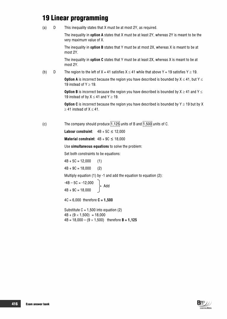
416 Exam answer bank
19 Linear programming (a) D This inequality states that X must be at most 2Y, as required.
The inequality in option A states that X must be at least 2Y, whereas 2Y is meant to be the very maximum value of X.
The inequality in option B states that Y must be at most 2X, whereas X is meant to be at most 2Y.
The inequality in option C states that Y must be at least 2X, whereas X is meant to be at most 2Y.
(b) D The region to the left of X = 41 satisfies X 41 while that above Y = 19 satisfies Y 19.
Option A is incorrect because the region you have described is bounded by X 41, but Y 19 instead of Y 19.
Option B is incorrect because the region you have described is bounded by X 41 and Y 19 instead of by X 41 and Y 19.
Option C is incorrect because the region you have described is bounded by Y 19 but by X 41 instead of X 41.
(c) The company should produce 1,125 units of B and 1,500 units of C.
Labour constraint: 4B + 5C 12,000
Material constraint: 4B + 9C 18,000
Use simultaneous equations to solve the problem:
Set both constraints to be equations:
4B + 5C = 12,000 (1)
4B + 9C = 18,000 (2)
Multiply equation (1) by -1 and add the equation to equation (2):
-4B – 5C = -12,000
4B + 9C = 18,000
4C = 6,000 therefore C = 1,500 Substitute C = 1,500 into equation (2)
4B + (9 1,500) = 18,000 4B = 18,000 – (9 1,500) therefore B = 1,125
Add

417
Index

418

Index 419
Note: Key Terms and their page references are given in bold.
ABC method of stores control, 132 Abnormal gain, 200 Abnormal loss, 200 Absorption base, 172 Absorption costing, 160 Absorption costing and marginal costing
compared, 188 Absorption of overheads, 171 Active cell, 90 Activity ratio, 140 Administration overhead, 45 Administration overheads, 180 Allocation, 162Attainable standards, 285 Attendance record, 149 Attributable fixed costs, 346 Average inventory, 124 Avoidable cost, 49, 345
Back-up, 104 Basic standard, 285 Batch, 246 Batch costing, 246 Bill of materials, 239 Bin cards, 119 Blanket absorption rates, 174 Blanket overhead absorption rate, 174Bonus schemes, 143 Breakeven, 324 Breakeven analysis, 324 Breakeven arithmetic, 326 Breakeven charts, 331 Breakeven point, 324, 326 Budget, 262Budget committee, 265 Budget manual, 264Budget period, 264 Budget preparation, 266 Bulk discounts, 128 By-products, 233
C/S (Contribution/sales) ratio, 325 Capacity ratio, 140 Cell, 90, 91 Cell protection., 105 Charts, 101 Clock card, 149 Coefficient of determination, 76 Column, 90 Column width, 97 Computers, 277
Conditions, 99 Constraints, 359 Continuous stocktaking, 121 Contribution, 184 Contribution breakeven charts, 334 Contribution charts, 331, 334 Contribution/sales (C/S) ratio, 325 Control, 29, 104, 109 Controllable cost, 49, 345 Corporate planning, 28 Correlation, 72Correlation and causation, 77 Correlation coefficient, 74Correlation in a time series, 75 Cost accounting department, 153 Cost accounts, 34 Cost behaviour and budgeting, 56 Cost behaviour and cost control, 56 Cost behaviour and decision making, 56 Cost behaviour and levels of activity, 56 Cost behaviour assumptions, 62 Cost behaviour patterns, 58 Cost behaviour principles, 57 Cost centres, 49 Cost objects, 50 Cost per service unit, 249 Cost plus pricing, 241 Cost units, 49 Costing methods, 242 Current standards, 285 Curvilinear variable costs, 60 CVP analysis, 324
Daily time sheets, 150 Data, 24 Day-rate system, 141 Decision making, 29 Decision-making problems, 351 Delete, 95 Delivery note, 116 Departmental absorption rates, 174 Deprival value of an asset, 350 Deteriorating inventory, 121 Direct costs, 42 Direct expenses, 44 Direct labour, 43 Direct labour budget, 268 Direct labour cost variances, 293 Direct material, 43 Direct material total variance, 290 Discretionary costs, 49 Distribution overhead, 45, 180

420 Index
EBQ, 128 Economic Batch Quantity (EBQ), 127 Economic Order Quantity (EOQ), 125 Editing data, 95 Effectiveness, 31 Efficiency, 31 Efficiency ratio, 140 EOQ (Economic Order Quantity), 125 Equivalent units, 211 Expected value, 81 Expenses, 43
F2 (edit), 95 Feasible area, 362 Feasible polygon, 362 FIFO (first in, first out) method, 215 Filling, 95 Financial accounts, 33 Financial information, 26 Fixed budget, 272 Fixed budgets, 272 Fixed costs, 48, 58, 346 Fixed overhead total variance, 297 Fixed overhead variances, 297 Fixed overhead volume capacity variance, 297 Fixed overhead volume efficiency variance, 297 Fixed overhead volume variance, 296, 297 Fixed production overhead variances, 295 Flexed budgets, 273 Flexible budget, 272, 273Forecast, 267 Formatting, 103 Formula bar, 91 Formulae, 92 Formulae with conditions, 100 Free inventory, 120 Function costing, 247 Function key F2 (edit), 95 Functional costs, 46
Go To (F5), 94 Goods received note (GRN), 116 Graphical solution to linear programming
problems, 361 Graphs, 101 Gridlines, 103 GRN, 116 Group bonus scheme, 145 Guaranteed minimum wage, 142
High day-rate system, 144 High-low method, 62 Holding costs, 122
Ideal standard, 285 Idle time, 152 Incentive schemes, 143 Incentive schemes involving shares, 146 Incremental costs, 344 Indirect cost, 42 Indirect expenses, 44 Indirect materials, 44 Indirect wages, 44 Individual bonus schemes, 145 Inequalities, 359 Information, 24 Inventory codes, 120 Inventory control, 114, 123 Inventory control levels, 122, 123 Inventory control systems, 118 Inventory costs, 122 Inventory count, 120 Inventory discrepancies, 121 Investment centre, 49, 51 Iso-profit lines, 365 Issue of materials, 117
Job, 238 Job cards, 150 Job cost cards, 239 Job cost information, 239 Job cost sheets, 239 Job costing, 242 Job costing and computerisation, 242 Job costing for internal services, 244 Job time, 150 Joint costs, 227 Joint products, 226 Joint products and common costs, 227 Joint products in process accounts, 230
Key budget factor, 266 Keyboard shortcut, 97
Labels, 102 Labour, 43 Labour budget, 268 Labour turnover, 153 Labour turnover rate, 154 Least squares method of linear regression
analysis, 77 Limitations of expected values, 87 Limiting budget factor, 266 Limiting factor, 351 Linear programming, 359 Linear programming and maximisation
problems, 366

Index 421
Linear programming and minimisation problems, 369
Lines of best fit, 77 Long-term planning, 28, 264 Long-term strategic planning, 28
Macros, 106 Management accounts, 33 Management control, 31 Management control system, 31 Margin of safety, 326 Marginal cost, 184 Marginal costing, 184, 187 Marginal costing and absorption costing
compared, 188 Marginal costing operating statement, 313 Marginal costing principles, 185 Material purchases budget, 270 Materials, 43 Materials codes, 120 Materials requisition note, 117 Materials returned note, 117 Materials returns, 117 Materials transfer note, 117 Materials transfers, 117 Materials variances and opening and closing
stock, 292 Maximum level, 123 Minimum level, 123 Mixed cost, 60
Negative correlation, 73Non-financial information, 26Non-linear variable costs, 60 Non-manufacturing overheads, 179 Non-negativity constraints, 359 Non-production overheads, 272 Non-relevant variable costs, 346 Normal loss, 200 Number format, 103
Objective, 27 Objective function, 360Obsolete inventory, 121 Operating statement, 310 Operation card, 151 Operational control, 31 Optimum production plan, 352Order cycling method of stores control, 131 Ordering costs, 122 Ordering materials, 115 Over-absorption, 176 Overhead, 42 Overhead absorption, 171, 173
Overhead absorption rate, 180, 296 Overhead apportionment, 164 Overheads, 160 Overtime, 43, 156 Overtime premium, 141
P/V (profit/volume) chart, 335 P/V ratio (profit/volume), 325 Pareto (80/20) distribution, 132 Partial correlation, 73 Passwords, 105 Payoff tables, 86 Perfect correlation, 73 Performance standard, 285 Period costs, 48 Periodic stocktaking, 121 Perpetual inventory, 121 Personnel department, 148 Piecework schemes, 142 Piecework ticket, 151 Planning, 27, 264Positive correlation, 73Power (^), 92 Predetermined overhead absorption rate, 171 Presentation of information to management, 35 Preventative costs, 154 Principal budget factor, 266Process costing, 198, 199 Process costing and closing work in progress,
211Process costing and losses, 200 Process costing and opening work in progress,
215weighted average cost method, 219
Process costing framework, 199 Procurement costs, 122 Production budget, 267, 268 Production planning department, 148 Production volume (P/V) ratio, 140 Productivity, 138 Productivity ratio, 140 Profit centre, 50 Profit/volume (P/V) chart, 331, 335 Profit/volume (P/V) ratio, 325 Profit-sharing schemes, 145 Purchase order, 115 Purchase requisition, 115
Range, 95 Receiving materials, 115 Rectification costs, 241 Regression, 77 Regression lines and time series, 79 Relevant cost, 344Relevant cost of labour, 348

422 Index
Relevant cost of materials, 347 Remuneration methods, 141 Reorder level, 123 Replacement costs, 154 Report, 35 Responsibility accounting, 263 Responsibility centre, 51 Revenue centres, 49, 50 Row, 90
Salaried labour, 151 Sales budget, 267 Sales variances, 308 Sales variances – significance, 309 Sales volume profit variance, 308 Scattergraph, 72Scrap, 205Selling overhead, 45, 180 Selling price variance, 308 Semi-fixed cost, 60 Semi-variable cost, 60 Separate absorption rates, 174 Service cost analysis, 249 Service cost analysis in service industry
situations, 252 Service costing, 247
unit cost measures, 248 Share option scheme, 146 Shift premium, 141 Short-term tactical planning, 28 Signing-in book, 149 Simultaneous equations, 370, 371 Slow-moving inventories, 121 Split off point, 226 Spreadsheet, 90 Spreadsheet formatting, 102 Spreadsheet formulae, 92 Spreadsheets and word processing software,
105Standard cost, 282 Standard costing, 277, 282, 284 Standard hour, 269 Standard hour of production, 139 Standard operation sheet, 287 Standard product specification, 286 Standard resource requirements, 286 Statements, 99
Step costs, 58 Stockout costs, 122 Storage of raw materials, 119 Stores ledger accounts, 119 Stores requisition, 117 Strategic information, 32 Strategic planning, 31 Strategy, 27 Strategy and organisational structure, 28 SUM button , 96 Sunk cost, 345
Tactical information, 32 Target profits, 327 Time work, 141 Timekeeping department, 148 Titles, 102 Toolbar, 97 Transfers and returns of materials, 117 Two-bin system of stores control, 132
Unavoidable costs, 49 Uncontrollable cost, 49, 345 Under-/over-absorbed overhead account, 178 Under-absorption, 176 Undoing actions (Ctrl + Z), 95
Value added, 146 Value added incentive schemes, 146 Variable costs, 48, 346 Variable overhead total variance, 294 Variable production overhead efficiency
variance, 295 Variable production overhead variances, 294 Variance, 275, 290, 308 Variances – interdependence, 303 Variances – reasons for, 301 Variances – significance, 302 Variances in a standard marginal costing
system, 313
Wages control account, 155 Wages department, 152 Weekly time sheets, 150
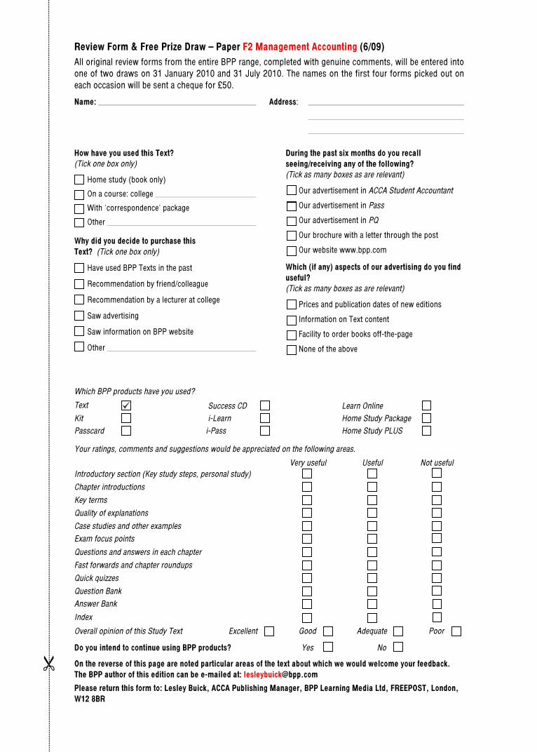
Review Form & Free Prize Draw – Paper F2 Management Accounting (6/09) All original review forms from the entire BPP range, completed with genuine comments, will be entered into one of two draws on 31 January 2010 and 31 July 2010. The names on the first four forms picked out on each occasion will be sent a cheque for £50.
Name: Address:
How have you used this Text? (Tick one box only)
Home study (book only)
On a course: college
With 'correspondence' package
Other
Why did you decide to purchase this Text? (Tick one box only)
Have used BPP Texts in the past
Recommendation by friend/colleague
Recommendation by a lecturer at college
Saw advertising
Saw information on BPP website
Other
During the past six months do you recall seeing/receiving any of the following? (Tick as many boxes as are relevant)
Our advertisement in ACCA Student Accountant
Our advertisement in Pass
Our advertisement in PQ
Our brochure with a letter through the post
Our website www.bpp.com
Which (if any) aspects of our advertising do you find useful?(Tick as many boxes as are relevant)
Prices and publication dates of new editions
Information on Text content
Facility to order books off-the-page
None of the above
Which BPP products have you used?
Text Success CD Learn Online Kit i-Learn Home Study Package Passcard i-Pass Home Study PLUS
Your ratings, comments and suggestions would be appreciated on the following areas.
Very useful Useful Not usefulIntroductory section (Key study steps, personal study)
Chapter introductions
Key terms
Quality of explanations
Case studies and other examples
Exam focus points
Questions and answers in each chapter
Fast forwards and chapter roundups
Quick quizzes
Question Bank
Answer Bank
Index
Overall opinion of this Study Text Excellent Good Adequate Poor
Do you intend to continue using BPP products? Yes No
On the reverse of this page are noted particular areas of the text about which we would welcome your feedback. The BPP author of this edition can be e-mailed at: [email protected]
Please return this form to: Lesley Buick, ACCA Publishing Manager, BPP Learning Media Ltd, FREEPOST, London, W12 8BR

Review Form & Free Prize Draw (continued)
TELL US WHAT YOU THINK
Please note any further comments and suggestions/errors below
Free Prize Draw Rules 1 Closing date for 31 January 2010 draw is 31 December 2009. Closing date for 31 July 2010 draw is 30 June 2010.
2 Restricted to entries with UK and Eire addresses only. BPP employees, their families and business associates are excluded.
3 No purchase necessary. Entry forms are available upon request from BPP Learning Media. No more than one entry per title, per person. Draw restricted to persons aged 16 and over.
4 Winners will be notified by post and receive their cheques not later than 6 weeks after the relevant draw date.
5 The decision of the promoter in all matters is final and binding. No correspondence will be entered into.