takeshi enomoto (kyoto university) enomoto… · takeshi enomoto (kyoto university)...

Quasi-uniform grids using a spherical helix

∗Takeshi Enomoto (Kyoto University)

∗[email protected]

8 April 2014

Acknowledgments: Dr S. Iga provided NICAM’s grids.

Workshop on the Partial Differential Equations on the Sphere 2014

Spherical Helix Takeshi Enomoto

Quasi-uniform grids on the sphere

Saff and Kuijlaars 1997

• Chemistry: Stable molecular structure (buckminsterfullerene)

• Physics: Location of identical point charges (J. J. Thomson’sproblem)

• Computation: Quadrature on the sphere and computationalcomplexity

• Botany: Distribution of pores on pollen (Tammes’s problem)

• Viral morphology, crystallography etc.

Workshop on the Partial Differential Equations on the Sphere 2014 1


Proposed approaches

• Geodesic grids (Williamson 1968; Sadourny et al. 1968)NB. Spring dynamics used in NICAM(Tomita et al. 2001; Tomita and Satoh 2004)

• Cubed sphere (Sadourny 1972; McGregor 1996)

• Reduced (Kurihara 1965; Hortal and Simmons 1991)

• Yin-Yang (Kageyama and Sato 2004; Purser 2004)

• Fibonacci (Swinbank and Purser 2006)

• Conformally mapped polyhedra (Purser and Rancic 2011)



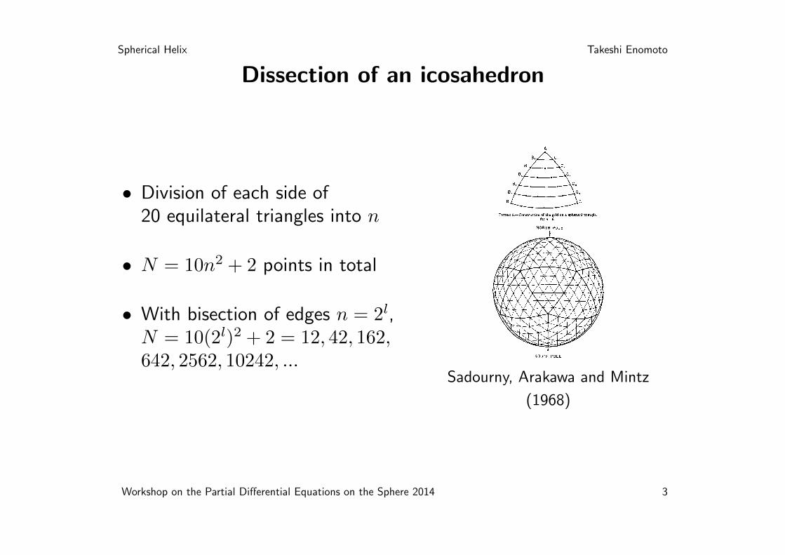
Dissection of an icosahedron

• Division of each side of20 equilateral triangles into n

• N = 10n2 + 2 points in total

• With bisection of edges n = 2l,N = 10(2l)2 + 2 = 12, 42, 162,642, 2562, 10242, ...

352

A

MONTHLY WEATHER REVIEW Vol. 96, No. 6

FIGURE 2.-Construction of the grid on a spherical triangle, for n=6.

NORTH POLE

t

4 SOUTH POLE

FIGURE 3.-Representation of the icosahedral-hexagonal grid, for n=6.

We divide the great circle arcs AB and AC into n equal arcs, to give the points B1, . . ., Bn-l, B, (coinciding with B) and Cl, . . ., C, (coinciding with 0. Then we take each great circle arc BiCi and divide it into i equal parts. The distance between adjacent grid points, in any direc- tion, varies by less than 10 percent over the spherical triangle.

If 0 is the center of the sphere, then we have to solve the linear system

n dd

OA . OBt=cos{ (i/n)AB), OB. OBi= cos { (1 -i/n)AB},

n A -

-A-

(OA, OB, OBJ=O.

FIGURE 4.-Indexing of a rhombus cell, for n=6.

The third equation expresses the condition that 0, A, B, Bi be coplanar. Here the radius of the sphere is equal to 1, and A 2 is the arc AB measured in radians.

In Cartesian coordinates this system is expressed by

xi+ YAY*+ ~ A Z F a~ 9

xBxi+ Y B y t + z B z t = a B , 1:: Yf Y A +o, XB Y B

h n where LU,=COS{ (;/..)AB} and aB=cos{ (I-i/n)AB). We solve this system for xt, y t , Zi.

Each point on the face or edge of one of the 20 faces of the icosahedron is now surrounded by six triangles and is therefore in the center of a hexagon. However, the points which form the vertices of the icosahedron are surrounded by only five triangles and therefore these 12 singular points are the centers of pentagons.

As shown in figure 3, the poles were chosen as two pentagonal points. The triangular faces of the icosahedron were arranged into 10 pairs of adjoining faces, forming 10 rhombuses; five around the North Pole and five around the South Pole, indexed from 1 to 10. The grid points inside each rhombus were indexed with two indices (i, j ) , as shown in the example of figure 4. The two Poles, where five rhombuses meet, are treated separately, but with the same finite difference scheme as the other vertices.

For the simplicity of the programming, all the fields were defined in a lOX(n+2)X(n+2) array. The over- lapping simplified the programming on the boundaries

Sadourny, Arakawa and Mintz

(1968)



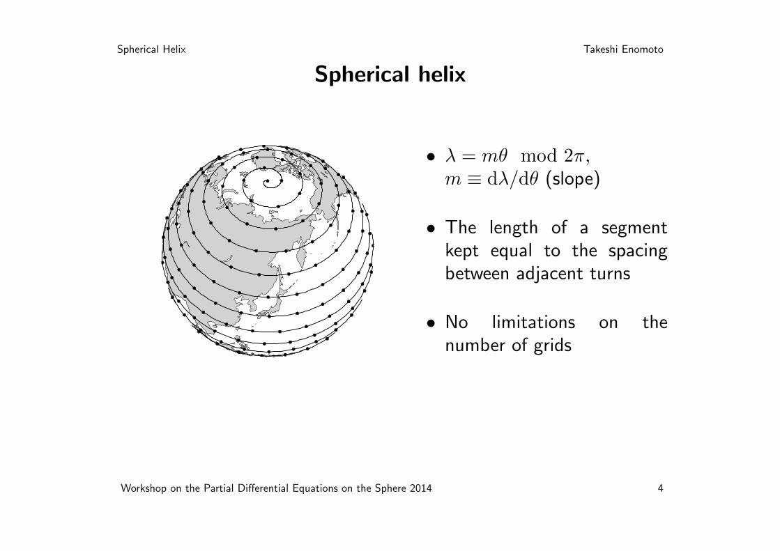
Spherical helix

• λ = mθ mod 2π,m ≡ dλ/dθ (slope)

• The length of a segmentkept equal to the spacingbetween adjacent turns

• No limitations on thenumber of grids



Spherical helix for spherical SOM(self-organizing maps)

Nishio, Altaf-Ul-Amin, Kurokawa and Kanaya (2006)

λ = 2√Nθ mod 2π (1)

Compute the spiral length L numerically and arrange neurons atequal intervals.

With L ≈ 2m for large m = 2√N the ratio between the adjacent

turns and the segment length is

2π

m

N

2m=Nπ

m2=π

46= 1 (2)



Generalized spiral points

Rakhmanov, Saff and Zhou (1994)

θk = arccos(hk), hk = −1 +2(k − 1)

N − 1, 1 ≤ k ≤ N (3)

λk =

(λk−1 +

c√N(1− h2k)

)mod 2π (4)

c = 3.6 <

(8√3

)1/2

= 3.809 (5)



The best packing on the sphere

Saff and Kuijlaars (1997)

• Hexagons except for 12 pentagons in the optimal arrangement.

• The area of the hexagon with the unit distance is√3/2.

• Ignoring the pentagonal cells, assume the sphere is covered byhexagonal Dirichlet cells

N

√3

2δ2N = 4π (6)

Thus the scaling factor is δN = (8π/√3)1/2N−1/2



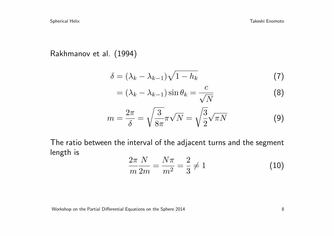
Rakhmanov et al. (1994)

δ = (λk − λk−1)√1− hk (7)

= (λk − λk−1) sin θk =c√N

(8)

m =2π

δ=

√3

8ππ√N =

√3

2

√πN (9)

The ratio between the interval of the adjacent turns and the segmentlength is

2π

m

N

2m=Nπ

m2=

2

36= 1 (10)



Spherical spiral

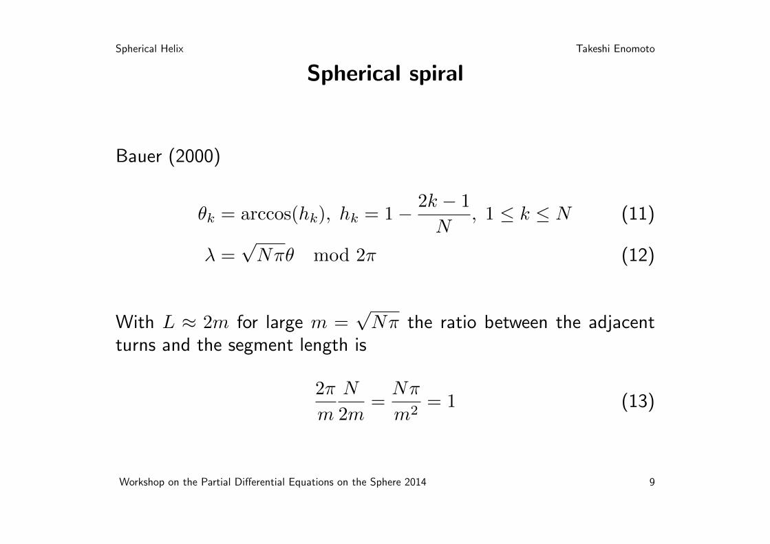
Bauer (2000)

θk = arccos(hk), hk = 1− 2k − 1

N, 1 ≤ k ≤ N (11)

λ =√Nπθ mod 2π (12)

With L ≈ 2m for large m =√Nπ the ratio between the adjacent

turns and the segment length is

2π

m

N

2m=Nπ

m2= 1 (13)



Analytically exact spiral

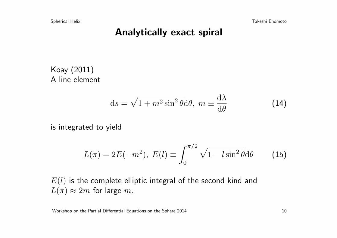
Koay (2011)A line element

ds =√1 +m2 sin2 θdθ, m ≡ dλ

dθ(14)

is integrated to yield

L(π) = 2E(−m2), E(l) ≡∫ π/2

0

√1− l sin2 θdθ (15)

E(l) is the complete elliptic integral of the second kind andL(π) ≈ 2m for large m.



Bauer (2000) Koay (2011)C.G. Koay / Journal of Computational Science 2 (2011) 88–91 89

Fig. 1. A surface element and a line element on the unit sphere.

leads to the following equation between ! and ":

" = m!. (3)

By substituting Eq. (3) into Eq. (2) and integrating Eq. (2) from0 to #, with 0 ≤ $ ≤ %, it is clear that the length of a segment ofthe spiral curve, denoted by S($), can be described precisely by theelliptic integral of the second kind as shown below:

S($) =!

2E(−m2) − E(% − $| − m2) : %/2 < $ ≤ %E($| − m2) : 0 ≤ $ ≤ %/2

(4)

Please note that our definition of the elliptic integral of the secondkind is given by the following expression, which is consistent withour previous work in [9]:

E("|m) =" "

0

#1 − m sin2(!) d!, 0 ≤ " ≤ %/2 (5)

E(m) ≡" %/2

0

#1 − m sin2(!) d!. (6)

Note also that E(m) is known as the complete elliptic integral ofthe second kind. Thus, the total length of the spiral curve is givenby 2E( − m2), i.e., S(%) = 2E( − m2). A well-known and interestingproperty noted and used by Bauer in his spiral scheme was thatS(%) asymptotically approaches 2m, denoted as S(%) ∼ 2m, becauseE( − m2) ∼ m for large m.

The second step is to divide the spiral curve into n segments ofequal length, which is S(%)/n, and then collect the center point ofeach segment along the spiral curve as an element of the desiredpoint set. To ensure that the spacing between adjacent turns of thespiral curve is not too close or too wide, we will keep the spacingbetween adjacent turns of the spiral curve to be equal to the lengthof a segment. This construction can be viewed from the point ofview of keeping the area enclosed by a segment and the spacingbetween adjacent turns of the spiral curve to be nearly equal forevery segment. Due to this simple relationship, " = m!, the spacingturns out to be 2%/m because as the spiral makes a complete turn," completes a cycle, which is 2%. Therefore, we have the criterion:

2%/m = S(%)n

(7)

or

m = 2n%S(%)

, (8)

m = n%E(−m2)

. (9)

It is interesting to note that Eq. (9) is a fixed point formula form and can be solved directly, see for example another exampleof fixed point formula in MR analysis of signals [7]. Specifically,let us define g(m) = n%/E( − m2) and iterate the function g on itselfsuch that |gi(m0) − mi−1| < ε for some nonnegative integer i and

Fig. 2. The new spiral point set of 88 points and its Voronoi tessellation.

a small fixed positive number ε, e.g., ε = 1.0 × 10−8. Note that gi

denotes composition of the function, g, i number of times, i.e.,gi(m0) ≡ g( · · · g(g(m0))). Any iterative scheme requires good start-ing values. Here, we use the asymptotic form of the solution whichis m∼

√n% because E( − m2) is asymptotically equal to m for large

m. The iteration based on Eq. (9) is highly inefficient and con-verges very slowly when m is large. This inefficiency can be gleanedfrom the first order derivative of Eq. (9) with respect to m. Specif-ically, although the absolute value of the derivative is less thanunity, which implies convergence, it approaches unity in the limitwhen m approaches infinity. For completeness, we have includedin Appendix A a highly efficient iterative approach based on New-ton’s method. For example, when n = 500 the fixed point methodand Newton’s method took 4884 and 4 iterations, respectively, atthe ε level of 1.0 × 10−8 and with the initial solution of m∼

√n%.

It is a significant gain in performance with at least three order ofmagnitude! Further examples are shown in Fig. 2.

Finally, the last step is to find the midpoint of each segment oncewe have the value of m. Based on the criterion stated above, weknow that the length of each segment is exactly 2%/m. Therefore,the point, #, at the end of the first spiral segment should satisfy thefollowing equation:

S($) = 2%/m. (10)

Similarly, we can find the midpoint of each segment but we willhave to solve for $j in the following equation:

S($j) = (2j − 1)%/m, j = 1, . . . , n. (11)

We define here an ‘inverse function’ of S, denoted by S−1, as a con-cise notation for expressing the solution above, i.e.,

$j = S−1((2j − 1)%/m), j = 1, . . . , n. (12)

Solving the nonlinear equation above requires reasonable initialsolutions. Here, we used $j = cos−1(1 − ((2j − 1)/n)) for j = 1, . . ., n asthe initial set of #j’s. This nonlinear equation can be solved via New-ton’s method of root-finding, which was mentioned in Appendix A.Please refer to Appendix B for the specific algorithm for the iterativemap of #.

It is clear then a desired spiral point set, {($j, ˚j)}nj=1, based

on the proposed scheme can be constructed by following thethree steps described above. Please note here that ˚j = m$j forall j. For completeness, the spiral points in Cartesian coordinates,



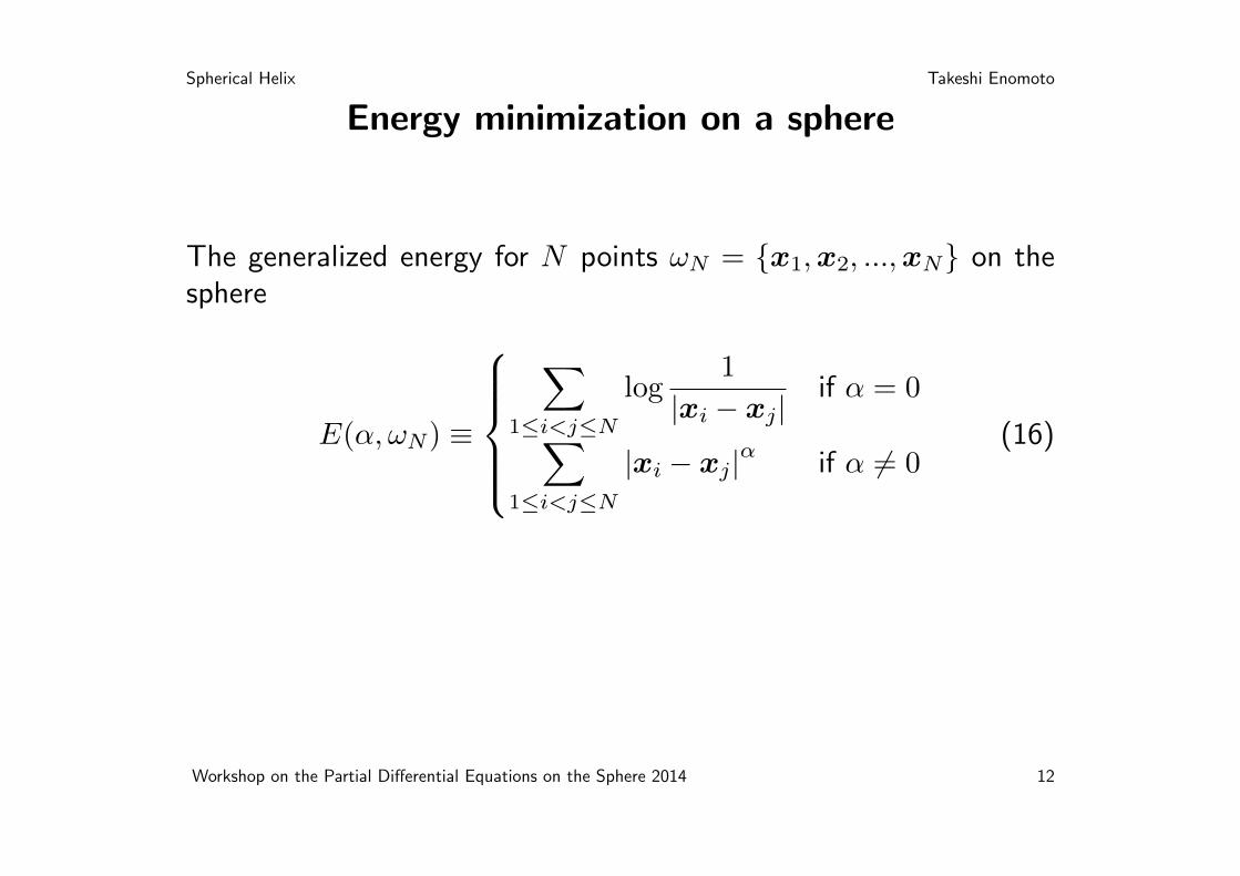
Energy minimization on a sphere

The generalized energy for N points ωN = {x1,x2, ...,xN} on thesphere

E(α, ωN) ≡

∑

1≤i<j≤N

log1

|xi − xj|if α = 0

∑

1≤i<j≤N

|xi − xj|α if α 6= 0(16)



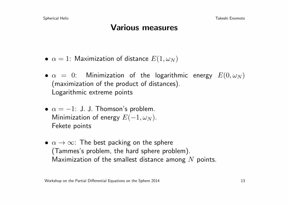
Various measures

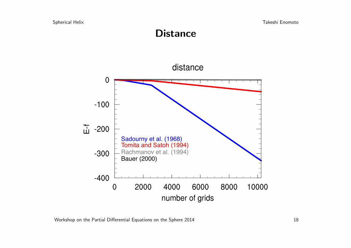
• α = 1: Maximization of distance E(1, ωN)

• α = 0: Minimization of the logarithmic energy E(0, ωN)(maximization of the product of distances).Logarithmic extreme points

• α = −1: J. J. Thomson’s problem.Minimization of energy E(−1, ωN).Fekete points

• α→∞: The best packing on the sphere(Tammes’s problem, the hard sphere problem).Maximization of the smallest distance among N points.



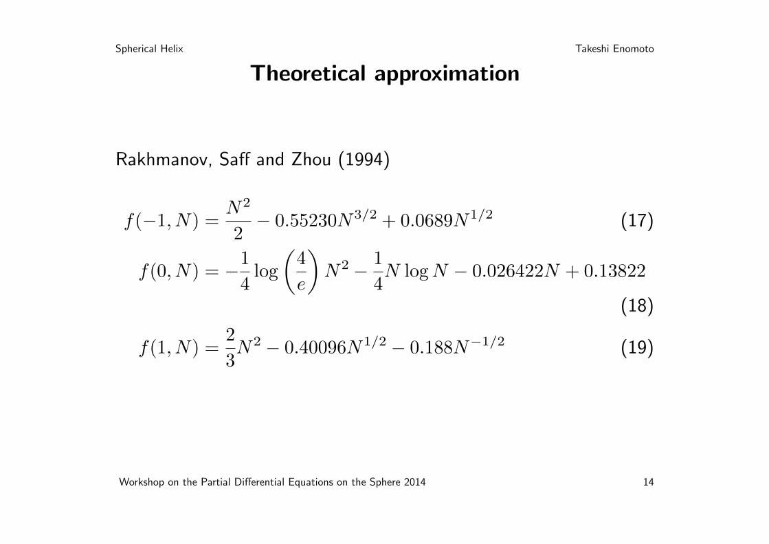
Theoretical approximation

Rakhmanov, Saff and Zhou (1994)

f(−1, N) =N2

2− 0.55230N3/2 + 0.0689N1/2 (17)

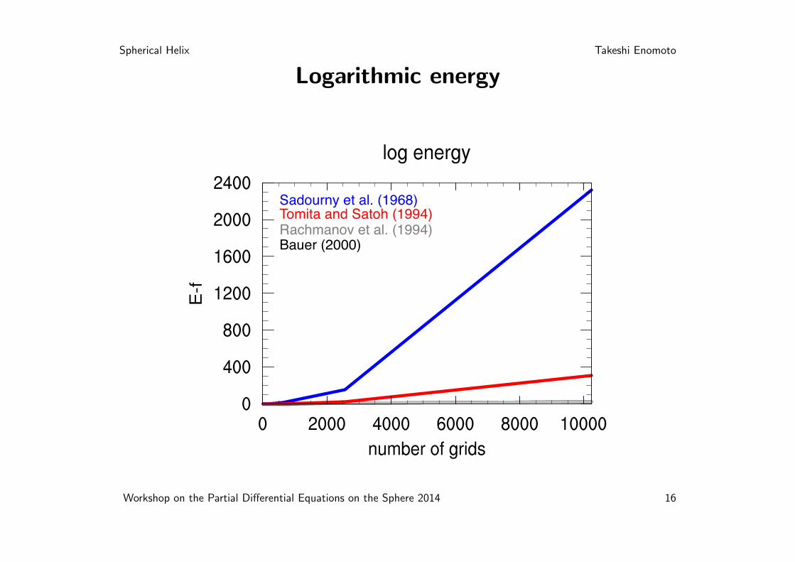
f(0, N) = −14log

(4

e

)N2 − 1

4N logN − 0.026422N + 0.13822

(18)

f(1, N) =2

3N2 − 0.40096N1/2 − 0.188N−1/2 (19)



Comparison of homogeneity

Compare norms with N = 12, 42, 162, 642, 2562, 10242

• Sadourny et al. (1968)

• Tomita and Satoh (1994)

• Rachmanov et al. (1994)

• Bauer (2000)



Logarithmic energy

Sadourny et al. (1968)Tomita and Satoh (1994)Rachmanov et al. (1994)Bauer (2000)



Energy




Distance




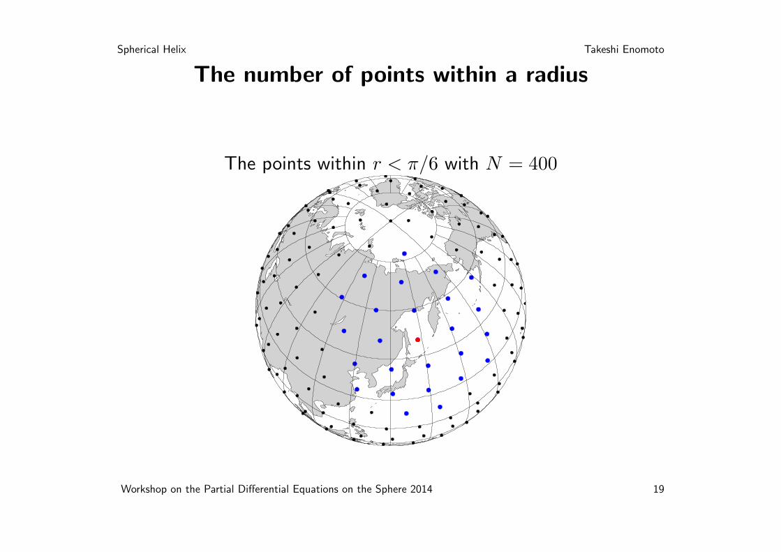
The number of points within a radius

The points within r < π/6 with N = 400



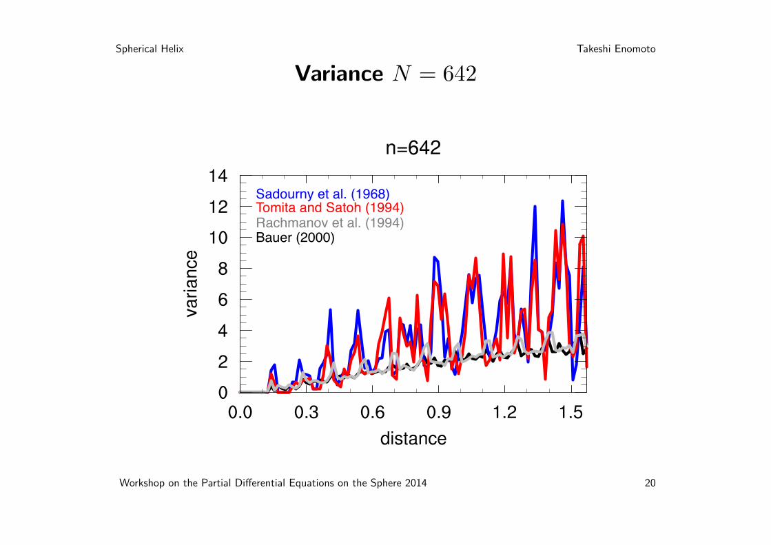
Variance N = 642




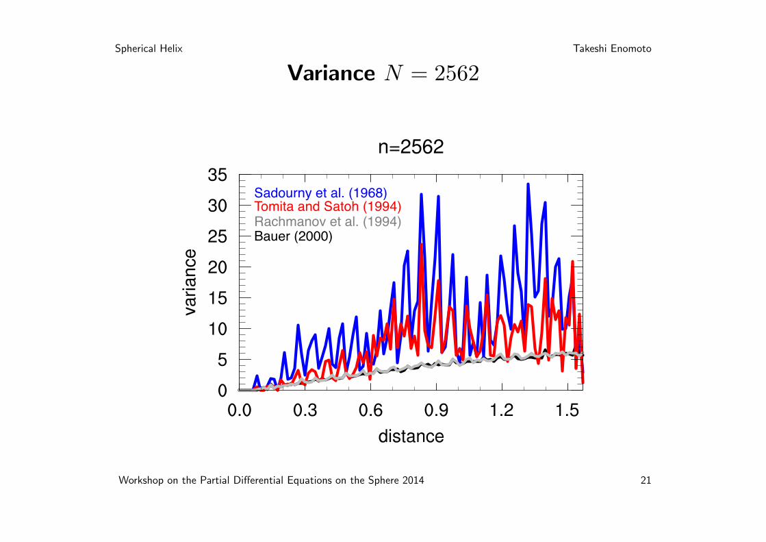
Variance N = 2562




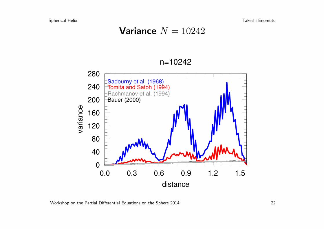
Variance N = 10242




“Untidiness”

Nishio et al. (2006)




Design choices

• Voronoi tessellation

• Approximate ME: quadrature with spherical harmonics

• 1D structure: interpolation. Semi-Lagrangian advection

• Weaknesses: 2D decomposition, local subdivision, ...



Summary

• Quasi-uniform grids can be easily generated with a spherical helix.

• Spherical helix grids are more uniform than geodesic grids invarious measures.

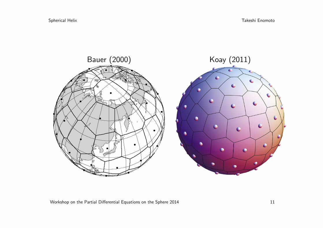
• The ratio between the adjacent turns and the segment length isunity in Bauer (2000) and Koay (2011) and not in Rakhmanov etal. (1994) and Nishio et al. (1997).

• The spiral length is approximated in Bauer (2000) and computedwith an iterative scheme without approximation in Koay (2011).

• Design choices remain for the use in dynamical cores


takeshi enomoto (kyoto university) enomoto… · takeshi enomoto (kyoto university)...

Documents