Taking Place Value Seriously:Arithmetic, Estimation, and Algebra

by Roger Howe, Yale Universityand Susanna S. Epp, DePaul University

Introduction and Summary

Arithmetic, first of nonnegative integers, then of decimal and common fractions, and later of rational expres-sions and functions, is a central theme in school mathematics. This article attempts to point out ways tomake the study of arithmetic more unified and more conceptual through a systematic emphasis on place-valuestructure in the base 10 number system. The article contains five sections.

Section one reviews the basic principles of base 10 notation and points out the sophisticated structureunderlying its amazing efficiency. Careful definitions are given for the basic constituents out of which numberswritten in base 10 notation are formed: digit , power of 10 , and single-place number. The idea of order ofmagnitude is also discussed, to prepare the way for considering relative sizes of numbers.

Section two discusses how base 10 notation enables efficient algorithms for addition, subtraction, mul-tiplication and division of nonnegative integers. The crucial point is that the main outlines of all theseprocedures are determined by the form of numbers written in base 10 notation together with the Rules ofArithmetic 1. Division plays an especially important role in the discussion because both of the two mainways to interpret numbers written in base 10 notation are connected with division. One way is to think ofthe base 10 expansion as the result of successive divisions-with-remainder by 10; the other way involves suc-cessive approximation by single-place numbers and provides the basis for the usual long-division algorithm.We observe that long division is a capstone arithmetic skill because it requires fluency with multiplication,subtraction, and estimation.

Section three discusses how base 10 notation can be extended from nonnegative integers to decimalfractions – that is, fractions whose denominators are powers of 10. The procedures for the arithmeticoperations also extend seamlessly. This is a practical reflection of the fact that the Law of Exponents can beextended to hold for all integers, not just nonnegative integers. The ease of computation when numbers arewritten in base 10 notation together with the efficient approximation properties discussed in sections 2D and5, make decimal fractions an efficient tool for practical computation, especially since numbers coming frommeasurements are known only approximately. The key features of base 10 notation have led to its heavyexploitation in machine computation.

Section four explores the connections of base 10 notation with algebra. It is suggested that decimalnumbers can be profitably thought of as “polynomials in 10,” and parallels between base 10 computationand computation with polynomials are illustrated. Understanding the basic structural aspects of base 10arithmetic can promote comfort with algebraic manipulation.

Section five discusses ordering, estimation, and approximation of numbers. For comparing numbers, theconcept of relative place value is a crucial idea. The corresponding idea for approximation is relative error .In many cases, both relative and absolute error can be controlled by using base 10 expansions. A key conceptis significant figure, and we note that relative accuracy of approximation improves rapidly – and relativeerror decreases rapidly – with the number of significant figures. In fact, it is usually unreasonable to expectto know a “real-world” number (meaning the result of a measurement) to more than three or four significantfigures, and often much less accuracy is enough. Failure to appreciate the limits of accuracy may be one of

1By the “Rules of Arithmetic,” we mean what mathematicians refer to as the Field Axioms, and what are often called“number properties,” or just “properties.” They are nine in number: four (Commutative, Associative, Identity and InverseRules) for addition, four parallel ones for multiplication, and the Distributive Rule to connect addition and multiplication.Other rules, such as “Invert and multiply,” or the formula for adding fractions, or the rules of signs for dealing with negativenumbers, can be deduced from these nine basic rules. See the Appendix for a more complete description of the Rules ofArithmetic.

1

the most pervasive forms of innumeracy: it affects many people who are for the most part quite comfortablewith numbers. Scientific notation, which focuses attention on the size of numbers and the accuracy to whichthey are known, is also discussed, as is the question of accuracy and estimation in arithmetic computation.

We hope that the issues addressed in this article will be of interest to a broad spectrum of mathematicseducators, a term we use inclusively, to comprise mathematics teachers at all levels, as well as others with aprofessional interest in mathematics education. Substantial effort has been devoted to making the contentsaccessible to a fairly wide audience, but what one reader may find obvious, another may find obscure, andvice versa. It is hoped that many readers can appreciate the broad message, that place value can serve asan organizing and unifying principle across the span of the elementary mathematics curriculum and beyond,and we beg our readers’ indulgence with parts that may seem either over- or under- elaborated, keeping inmind that other readers may see them in the opposite light.

Acknowledgements: The authors are grateful for comments on earlier drafts of this article from theMathematics School Study Group committee members, from Johnny Lott and his associates in NCTM andASSM, especially Gail Englert, Bonny Hagelberger, and Mari Muri, and from Scott Baldridge, ThomasRoby, and Kristin Ulmann. Thanks to Mel Delvecchio and W. Barker for vital production help.

1. The Base 10 System: Single-place Numbers, Expanded Form, and Order ofMagnitude

Our ordinary base 10 system is a highly sophisticated method for writing numbers efficiently. It uses only10 symbols (the digits: 0,1,2,3,4,5,6,7,8,9), arranged in carefully structured groups, to express any number.Further, it does so with impressive economy. To express the total human population of the world wouldrequire only a ten-digit number, needing just a few seconds to write.

The efficiency of the base 10 system is possible because of its systematic use of mathematical structure.We hope that making more aspects of this structure explicit will increase conceptual understanding andimprove computational flexibility, thereby helping to make mathematics instruction more effective. It mayalso promote numeracy by making students more sensitive to order of magnitude, and to the estimationcapabilities of place-value, or base 10, notation. Finally, it can illuminate the parallels between arithmeticand algebra, thus making arithmetic a preparation for algebra, rather than the impediment that it sometimesappears to be [KSF, Ch.8].

All the numbers discussed in this section and the next will be nonnegative integers. When such a numberis written in base 10 notation, we will say that it is in base 10 form. A number in base 10 form is implicitlybroken up into a sum of numbers of a special type. For example, consider

7, 452 = 7, 000 + 400 + 50 + 2.

The right-hand side of this equation is usually called the expanded form of the number, and we often saythat the digit 7 is in the thousands place, 4 is in the hundreds place, 5 is in the tens place, and 2 is inthe ones place. Although the concept of expanded form is mentioned in state mathematics standards, thisarticle explores what would follow from making it central to arithmetic instruction.

Each of the addends in the expanded form of a number will be called a single-place number . Thuseach single-place number can be written as a digit – possibly 0 – times a power of 10 (that is, a productof a certain number of 10’s).2 The following display shows the various representations for the single-placenumbers in the previous example:

7, 000 = 7× 1000 = 7× (10× 10× 10) = 7× 103

400 = 4× 100 = 4× (10× 10) = 4× 102

50 = 5× 10 = 5× 101

2 = 2× 1 2× 100.

2Exponential notation is discussed in section 2C.

2

The order of magnitude of a (non-zero) single-place number is the number of zeroes used towrite it, or, equivalently, it is the exponent of 10 when the number is written using exponential notation.For example, since 7, 000 = 7 × 103 and since 400 = 4 × 102, the order of magnitude of 7,000 is 3 and theorder of magnitude of 400 is 2.

When a positive integer is written in base 10 form, its leading component is its largest single-placecomponent, and its order of magnitude is the order of magnitude of its leading component. For instance,because the leading component of 7,452 is 7,000, the order of magnitude of 7,452 is 3. When the meaning isclear, we will sometimes refer to a number’s “magnitude” rather than to its “order of magnitude.”

A key point about expanded form is that no two single-place components of an integer have the sameorder of magnitude. In fact, this property characterizes expanded form: A sum of single-place componentsis the expanded form of a number exactly when

a. it involves exactly one component of each order of magnitude up to the magnitude of the number, and

b. the components are arranged from left to right in descending order according to their orders of mag-nitude.

It follows that the expanded form of an integer is unique.Given the terminology we have introduced, we can say either that in the number 7,452 the digit 4 is in

the hundreds place or that the single-place component with magnitude 2 in 7,452 is 400. Note, however,that although 7,052 does not have a single-place component with magnitude 2, we say that it has a zero inthe hundreds place.

2. Single-place Numbers and the Algorithms of Arithmetic

The fact that numbers in base 10 form are sums has a pervasive influence on the methods for computingwith them. Indeed, the usual procedures for adding, subtracting, multiplying, and dividing two such numbersare obtained by applying the Rules of Arithmetic to the sums of their single-place components. The Rules ofArithmetic play the critical role of reducing an arithmetic computation involving two numbers to a collectionof simple single-digit computations involving the single-place components of the numbers.

2A. Addition

We call the basic strategy for adding two numbers in base 10 form the addition algorithm. It consists ofthree steps:

1. Break each of the numbers (the “addends”) into its single-place components.

2. Add the corresponding components for each order of magnitude. If the component for an order ofmagnitude of an addend is missing, it is treated as if it were zero.

3. Recombine the sums from step 2 into a number in base 10 form. (The details of this step give rise tothe trickier parts of the algorithm.)

Here is a simple example:

294 + 603 = (200 + 90 + 4) + (600 + 3) by breaking each addend into its single-place components

= (200 + 600) + 90) + (4 + 3) by grouping the single-place components by order of magnitude

= 800 + 90 + 7 by adding components for each order of magnitude

= 897 by recombining the single-place components into a base 10 number.

To be able to analyze the steps of the addition algorithm, we need to develop some preliminary ideas.

3

Basic Rules for Addition: The basic strategy is justified by means of the two most basic rules of addition,the Commutative Rule and the Associative Rule, together with the Distributive Rule, which is the rule thatinvolves both addition and multiplication.

The Commutative Rule for Addition : The value of a sum does not depend on the orderof the addends. In other words, for any two nonnegative integers, a and b,

a + b = b + a.

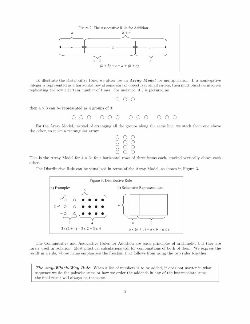
The Associative Rule for Addition : When adding three numbers, the value of the sumdoes not depend on the way the numbers are combined into pairwise sums. More precisely,for any three nonnegative integers a, b, and c,

(a + b) + c = a + (b + c).

The Distributive Rule: The product of one nonnegative integer times a sum of two othersis obtained by adding the first number times the second plus the first number times the third.More precisely, for any nonnegative integers a, b, and c,

a× (b + c) = a× b + a× c.

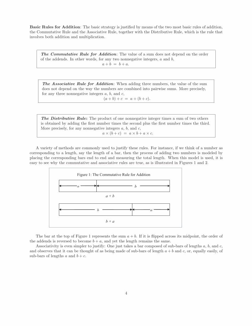
A variety of methods are commonly used to justify these rules. For instance, if we think of a number ascorresponding to a length, say the length of a bar, then the process of adding two numbers is modeled byplacing the corresponding bars end to end and measuring the total length. When this model is used, it iseasy to see why the commutative and associative rules are true, as is illustrated in Figures 1 and 2.

a b

b a

Figure 1: The Commutative Rule for Addition

a + b

b + a

The bar at the top of Figure 1 represents the sum a + b. If it is flipped across its midpoint, the order ofthe addends is reversed to become b + a, and yet the length remains the same.

Associativity is even simpler to justify: One just takes a bar composed of sub-bars of lengths a, b, and c,and observes that it can be thought of as being made of sub-bars of length a + b and c, or, equally easily, ofsub-bars of lengths a and b + c.

4

a b

(a + b) + c = a + (b + c)

Figure 2: The Associative Rule for Addition

c

a b + c

a + b c

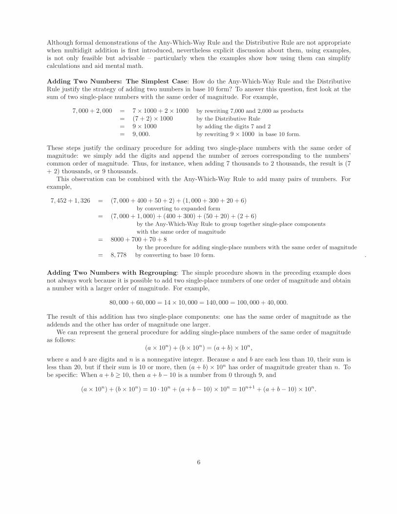
To illustrate the Distributive Rule, we often use an Array Model for multiplication. If a nonnegativeinteger is represented as a horizontal row of some sort of object, say small circles, then multiplication involvesreplicating the row a certain number of times. For instance, if 3 is pictured as

© © ©

then 4× 3 can be represented as 4 groups of 3:

© © © © © © © © © © © © .

For the Array Model, instead of arranging all the groups along the same line, we stack them one abovethe other, to make a rectangular array:

© © ©© © ©© © ©© © ©

This is the Array Model for 4 × 3: four horizontal rows of three items each, stacked vertically above eachother.

The Distributive Rule can be visualized in terms of the Array Model, as shown in Figure 3.

Figure 3: Distributive Rule

b) Schematic Representation:

a

b c

a X (b + c) = a X b + a X c 3 X (2 + 4) = 3 X 2 + 3 X 4

a) Example: 6

2 4

3

○ ○ ○ ○ ○ ○

● ● ● ● ● ● ● ● ● ● ● ●

The Commutative and Associative Rules for Addition are basic principles of arithmetic, but they arerarely used in isolation. Most practical calculations call for combinations of both of them. We express theresult in a rule, whose name emphasizes the freedom that follows from using the two rules together.

The Any-Which-Way Rule: When a list of numbers is to be added, it does not matter in whatsequence we do the pairwise sums or how we order the addends in any of the intermediate sums:the final result will always be the same.

5

Although formal demonstrations of the Any-Which-Way Rule and the Distributive Rule are not appropriatewhen multidigit addition is first introduced, nevertheless explicit discussion about them, using examples,is not only feasible but advisable – particularly when the examples show how using them can simplifycalculations and aid mental math.

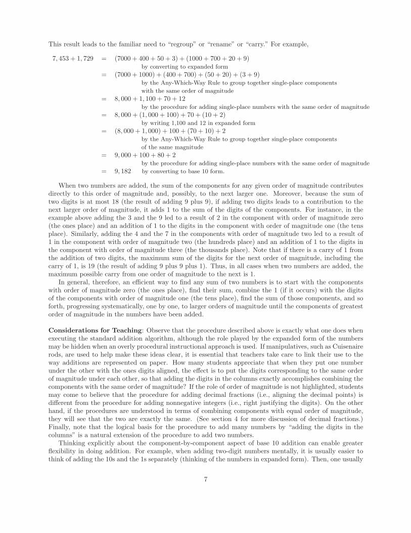
Adding Two Numbers: The Simplest Case: How do the Any-Which-Way Rule and the DistributiveRule justify the strategy of adding two numbers in base 10 form? To answer this question, first look at thesum of two single-place numbers with the same order of magnitude. For example,

7, 000 + 2, 000 = 7× 1000 + 2× 1000 by rewriting 7,000 and 2,000 as products

= (7 + 2)× 1000 by the Distributive Rule

= 9× 1000 by adding the digits 7 and 2

= 9, 000. by rewriting 9× 1000 in base 10 form.

These steps justify the ordinary procedure for adding two single-place numbers with the same order ofmagnitude: we simply add the digits and append the number of zeroes corresponding to the numbers’common order of magnitude. Thus, for instance, when adding 7 thousands to 2 thousands, the result is (7+ 2) thousands, or 9 thousands.

This observation can be combined with the Any-Which-Way Rule to add many pairs of numbers. Forexample,

7, 452 + 1, 326 = (7, 000 + 400 + 50 + 2) + (1, 000 + 300 + 20 + 6)by converting to expanded form

= (7, 000 + 1, 000) + (400 + 300) + (50 + 20) + (2 + 6)by the Any-Which-Way Rule to group together single-place components

with the same order of magnitude

= 8000 + 700 + 70 + 8by the procedure for adding single-place numbers with the same order of magnitude

= 8, 778 by converting to base 10 form. .

Adding Two Numbers with Regrouping: The simple procedure shown in the preceding example doesnot always work because it is possible to add two single-place numbers of one order of magnitude and obtaina number with a larger order of magnitude. For example,

80, 000 + 60, 000 = 14× 10, 000 = 140, 000 = 100, 000 + 40, 000.

The result of this addition has two single-place components: one has the same order of magnitude as theaddends and the other has order of magnitude one larger.

We can represent the general procedure for adding single-place numbers of the same order of magnitudeas follows:

(a× 10n) + (b× 10n) = (a + b)× 10n,

where a and b are digits and n is a nonnegative integer. Because a and b are each less than 10, their sum isless than 20, but if their sum is 10 or more, then (a + b) × 10n has order of magnitude greater than n. Tobe specific: When a + b ≥ 10, then a + b− 10 is a number from 0 through 9, and

(a× 10n) + (b× 10n) = 10 · 10n + (a + b− 10)× 10n = 10n+1 + (a + b− 10)× 10n.

6

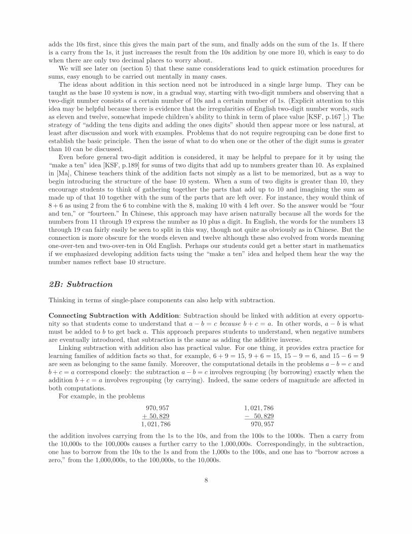
This result leads to the familiar need to “regroup” or “rename” or “carry.” For example,

7, 453 + 1, 729 = (7000 + 400 + 50 + 3) + (1000 + 700 + 20 + 9)by converting to expanded form

= (7000 + 1000) + (400 + 700) + (50 + 20) + (3 + 9)by the Any-Which-Way Rule to group together single-place components

with the same order of magnitude

= 8, 000 + 1, 100 + 70 + 12by the procedure for adding single-place numbers with the same order of magnitude

= 8, 000 + (1, 000 + 100) + 70 + (10 + 2)by writing 1,100 and 12 in expanded form

= (8, 000 + 1, 000) + 100 + (70 + 10) + 2by the Any-Which-Way Rule to group together single-place components

of the same magnitude

= 9, 000 + 100 + 80 + 2by the procedure for adding single-place numbers with the same order of magnitude

= 9, 182 by converting to base 10 form.

When two numbers are added, the sum of the components for any given order of magnitude contributesdirectly to this order of magnitude and, possibly, to the next larger one. Moreover, because the sum oftwo digits is at most 18 (the result of adding 9 plus 9), if adding two digits leads to a contribution to thenext larger order of magnitude, it adds 1 to the sum of the digits of the components. For instance, in theexample above adding the 3 and the 9 led to a result of 2 in the component with order of magnitude zero(the ones place) and an addition of 1 to the digits in the component with order of magnitude one (the tensplace). Similarly, adding the 4 and the 7 in the components with order of magnitude two led to a result of1 in the component with order of magnitude two (the hundreds place) and an addition of 1 to the digits inthe component with order of magnitude three (the thousands place). Note that if there is a carry of 1 fromthe addition of two digits, the maximum sum of the digits for the next order of magnitude, including thecarry of 1, is 19 (the result of adding 9 plus 9 plus 1). Thus, in all cases when two numbers are added, themaximum possible carry from one order of magnitude to the next is 1.

In general, therefore, an efficient way to find any sum of two numbers is to start with the componentswith order of magnitude zero (the ones place), find their sum, combine the 1 (if it occurs) with the digitsof the components with order of magnitude one (the tens place), find the sum of those components, and soforth, progressing systematically, one by one, to larger orders of magnitude until the components of greatestorder of magnitude in the numbers have been added.

Considerations for Teaching: Observe that the procedure described above is exactly what one does whenexecuting the standard addition algorithm, although the role played by the expanded form of the numbersmay be hidden when an overly procedural instructional approach is used. If manipulatives, such as Cuisenairerods, are used to help make these ideas clear, it is essential that teachers take care to link their use to theway additions are represented on paper. How many students appreciate that when they put one numberunder the other with the ones digits aligned, the effect is to put the digits corresponding to the same orderof magnitude under each other, so that adding the digits in the columns exactly accomplishes combining thecomponents with the same order of magnitude? If the role of order of magnitude is not highlighted, studentsmay come to believe that the procedure for adding decimal fractions (i.e., aligning the decimal points) isdifferent from the procedure for adding nonnegative integers (i.e., right justifying the digits). On the otherhand, if the procedures are understood in terms of combining components with equal order of magnitude,they will see that the two are exactly the same. (See section 4 for more discussion of decimal fractions.)Finally, note that the logical basis for the procedure to add many numbers by “adding the digits in thecolumns” is a natural extension of the procedure to add two numbers.

Thinking explicitly about the component-by-component aspect of base 10 addition can enable greaterflexibility in doing addition. For example, when adding two-digit numbers mentally, it is usually easier tothink of adding the 10s and the 1s separately (thinking of the numbers in expanded form). Then, one usually

7

adds the 10s first, since this gives the main part of the sum, and finally adds on the sum of the 1s. If thereis a carry from the 1s, it just increases the result from the 10s addition by one more 10, which is easy to dowhen there are only two decimal places to worry about.

We will see later on (section 5) that these same considerations lead to quick estimation procedures forsums, easy enough to be carried out mentally in many cases.

The ideas about addition in this section need not be introduced in a single large lump. They can betaught as the base 10 system is now, in a gradual way, starting with two-digit numbers and observing that atwo-digit number consists of a certain number of 10s and a certain number of 1s. (Explicit attention to thisidea may be helpful because there is evidence that the irregularities of English two-digit number words, suchas eleven and twelve, somewhat impede children’s ability to think in term of place value [KSF, p.167 ].) Thestrategy of “adding the tens digits and adding the ones digits” should then appear more or less natural, atleast after discussion and work with examples. Problems that do not require regrouping can be done first toestablish the basic principle. Then the issue of what to do when one or the other of the digit sums is greaterthan 10 can be discussed.

Even before general two-digit addition is considered, it may be helpful to prepare for it by using the“make a ten” idea [KSF, p.189] for sums of two digits that add up to numbers greater than 10. As explainedin [Ma], Chinese teachers think of the addition facts not simply as a list to be memorized, but as a way tobegin introducing the structure of the base 10 system. When a sum of two digits is greater than 10, theyencourage students to think of gathering together the parts that add up to 10 and imagining the sum asmade up of that 10 together with the sum of the parts that are left over. For instance, they would think of8 + 6 as using 2 from the 6 to combine with the 8, making 10 with 4 left over. So the answer would be “fourand ten,” or “fourteen.” In Chinese, this approach may have arisen naturally because all the words for thenumbers from 11 through 19 express the number as 10 plus a digit. In English, the words for the numbers 13through 19 can fairly easily be seen to split in this way, though not quite as obviously as in Chinese. But theconnection is more obscure for the words eleven and twelve although these also evolved from words meaningone-over-ten and two-over-ten in Old English. Perhaps our students could get a better start in mathematicsif we emphasized developing addition facts using the “make a ten” idea and helped them hear the way thenumber names reflect base 10 structure.

2B: Subtraction

Thinking in terms of single-place components can also help with subtraction.

Connecting Subtraction with Addition: Subtraction should be linked with addition at every opportu-nity so that students come to understand that a − b = c because b + c = a. In other words, a − b is whatmust be added to b to get back a. This approach prepares students to understand, when negative numbersare eventually introduced, that subtraction is the same as adding the additive inverse.

Linking subtraction with addition also has practical value. For one thing, it provides extra practice forlearning families of addition facts so that, for example, 6 + 9 = 15, 9 + 6 = 15, 15− 9 = 6, and 15 − 6 = 9are seen as belonging to the same family. Moreover, the computational details in the problems a− b = c andb + c = a correspond closely: the subtraction a− b = c involves regrouping (by borrowing) exactly when theaddition b + c = a involves regrouping (by carrying). Indeed, the same orders of magnitude are affected inboth computations.

For example, in the problems

970, 957 1, 021, 786+ 50, 829 − 50, 8291, 021, 786 970, 957

the addition involves carrying from the 1s to the 10s, and from the 100s to the 1000s. Then a carry fromthe 10,000s to the 100,000s causes a further carry to the 1,000,000s. Correspondingly, in the subtraction,one has to borrow from the 10s to the 1s and from the 1,000s to the 100s, and one has to “borrow across azero,” from the 1,000,000s, to the 100,000s, to the 10,000s.

8

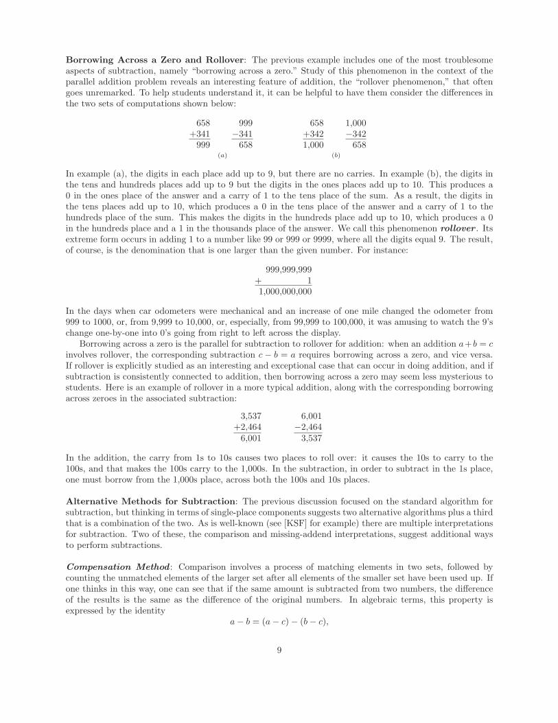
Borrowing Across a Zero and Rollover: The previous example includes one of the most troublesomeaspects of subtraction, namely “borrowing across a zero.” Study of this phenomenon in the context of theparallel addition problem reveals an interesting feature of addition, the “rollover phenomenon,” that oftengoes unremarked. To help students understand it, it can be helpful to have them consider the differences inthe two sets of computations shown below:

658 999+341 −341

999 658(a)

658 1,000+342 −3421,000 658

(b)

In example (a), the digits in each place add up to 9, but there are no carries. In example (b), the digits inthe tens and hundreds places add up to 9 but the digits in the ones places add up to 10. This produces a0 in the ones place of the answer and a carry of 1 to the tens place of the sum. As a result, the digits inthe tens places add up to 10, which produces a 0 in the tens place of the answer and a carry of 1 to thehundreds place of the sum. This makes the digits in the hundreds place add up to 10, which produces a 0in the hundreds place and a 1 in the thousands place of the answer. We call this phenomenon rollover . Itsextreme form occurs in adding 1 to a number like 99 or 999 or 9999, where all the digits equal 9. The result,of course, is the denomination that is one larger than the given number. For instance:

999,999,999+ 11,000,000,000

In the days when car odometers were mechanical and an increase of one mile changed the odometer from999 to 1000, or, from 9,999 to 10,000, or, especially, from 99,999 to 100,000, it was amusing to watch the 9’schange one-by-one into 0’s going from right to left across the display.

Borrowing across a zero is the parallel for subtraction to rollover for addition: when an addition a+b = cinvolves rollover, the corresponding subtraction c − b = a requires borrowing across a zero, and vice versa.If rollover is explicitly studied as an interesting and exceptional case that can occur in doing addition, and ifsubtraction is consistently connected to addition, then borrowing across a zero may seem less mysterious tostudents. Here is an example of rollover in a more typical addition, along with the corresponding borrowingacross zeroes in the associated subtraction:

3,537 6,001+2,464 −2,464

6,001 3,537

In the addition, the carry from 1s to 10s causes two places to roll over: it causes the 10s to carry to the100s, and that makes the 100s carry to the 1,000s. In the subtraction, in order to subtract in the 1s place,one must borrow from the 1,000s place, across both the 100s and 10s places.

Alternative Methods for Subtraction: The previous discussion focused on the standard algorithm forsubtraction, but thinking in terms of single-place components suggests two alternative algorithms plus a thirdthat is a combination of the two. As is well-known (see [KSF] for example) there are multiple interpretationsfor subtraction. Two of these, the comparison and missing-addend interpretations, suggest additional waysto perform subtractions.

Compensation Method : Comparison involves a process of matching elements in two sets, followed bycounting the unmatched elements of the larger set after all elements of the smaller set have been used up. Ifone thinks in this way, one can see that if the same amount is subtracted from two numbers, the differenceof the results is the same as the difference of the original numbers. In algebraic terms, this property isexpressed by the identity

a− b = (a− c)− (b− c),

9

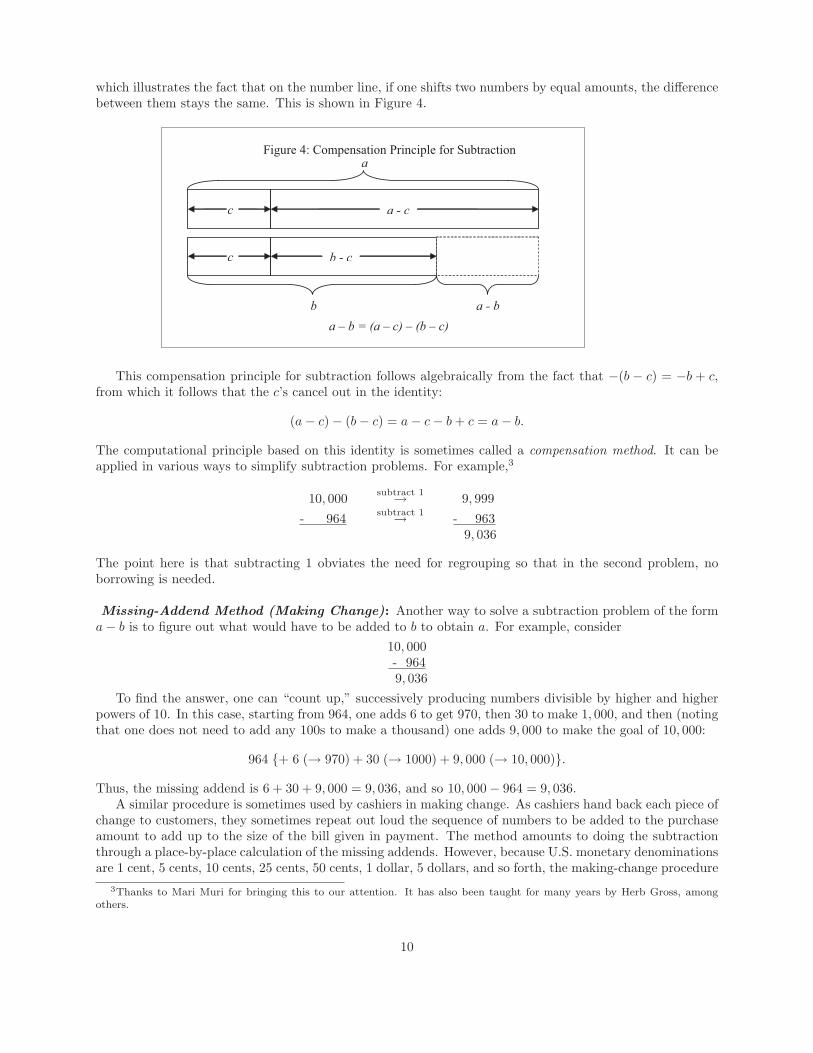
which illustrates the fact that on the number line, if one shifts two numbers by equal amounts, the differencebetween them stays the same. This is shown in Figure 4.

c a - c

a – b = (a – c) – (b – c)

Figure 4: Compensation Principle for Subtraction a

a + b c c b - c

b a - b

This compensation principle for subtraction follows algebraically from the fact that −(b − c) = −b + c,from which it follows that the c’s cancel out in the identity:

(a− c)− (b− c) = a− c− b + c = a− b.

The computational principle based on this identity is sometimes called a compensation method. It can beapplied in various ways to simplify subtraction problems. For example,3

10, 000 subtract 1→ 9, 999- 964 subtract 1→ - 963

9, 036

The point here is that subtracting 1 obviates the need for regrouping so that in the second problem, noborrowing is needed.

Missing-Addend Method (Making Change): Another way to solve a subtraction problem of the forma− b is to figure out what would have to be added to b to obtain a. For example, consider

10, 000- 9649, 036

To find the answer, one can “count up,” successively producing numbers divisible by higher and higherpowers of 10. In this case, starting from 964, one adds 6 to get 970, then 30 to make 1, 000, and then (notingthat one does not need to add any 100s to make a thousand) one adds 9, 000 to make the goal of 10, 000:

964 {+ 6 (→ 970) + 30 (→ 1000) + 9, 000 (→ 10, 000)}.

Thus, the missing addend is 6 + 30 + 9, 000 = 9, 036, and so 10, 000− 964 = 9, 036.A similar procedure is sometimes used by cashiers in making change. As cashiers hand back each piece of

change to customers, they sometimes repeat out loud the sequence of numbers to be added to the purchaseamount to add up to the size of the bill given in payment. The method amounts to doing the subtractionthrough a place-by-place calculation of the missing addends. However, because U.S. monetary denominationsare 1 cent, 5 cents, 10 cents, 25 cents, 50 cents, 1 dollar, 5 dollars, and so forth, the making-change procedure

3Thanks to Mari Muri for bringing this to our attention. It has also been taught for many years by Herb Gross, amongothers.

10

is applied to subtractions from single-place numbers as well as from powers of ten. For example, makingchange for a purchase of $2.85 from a $5 payment, amounts to computing $5.00 − $2.85. One would startfrom $2.85, then add 5 cents to reach $2.90, 10 cents to reach $3.00, and finally $2.00 to reach $5.00:

$2.85 {+ $0.05 (→ $2.90) + $0.10 (→ $3.00) + $2.00 (→ $5.00)}.So the change is $5.00− $2.85 = $0.05 + $0.10 + $2.00 = $2.15. In giving you the change, the cashier mightstart by saying, “Two-eighty-five,” and then say, in handing you first the nickel, then the dime, and finallythe two dollars, “Two-eighty-five, two-ninety, three dollars, five dollars.”

A Combination Method : Another subtraction procedure systematically utilizes place-by-place compen-sation to reduce a problem to a simpler one, in which, for each magnitude, the digit of either the subtrahendor the minuend is zero. The result is that the initial problem is decomposed into a set of missing-addendproblems.

To be specific:

Given a subtraction c− a of numbers in base 10 form, for each orderof magnitude, subtract from both numbers the smaller of thebase 10 components of c and a with that magnitude. The result isan equivalent subtraction problem in which, for each order ofmagnitude, only one of the addends has a non-zero component.

For example, consider the problem of computing 83 − 26. The two components in the ones place (i.e.,with magnitude zero) are 3 and 6, so 3 is subtracted from both 83 and 26 to obtain the equivalent problem80− 23. The components in the tens place (i.e., of magnitude one) are 80 and 20, so 20 is subtracted fromboth 80 and 23 to obtain the equivalent problem 60 − 03, which is computed using the missing-addendmethod, i.e., by answering the question “What must be added to 3 to obtain 60?”:

83 subtract 3→ 80 subtract 20→ 60- 26 subtract 3→ - 23 subtract 20→ - 03

57

Now let’s look at a three-digit problem where borrowing across a zero would ordinarily be needed. Tocompute 204−9, we note that the components in the ones place are 4 and 9, so we subtract 4 from both 204and 9 to obtain the equivalent problem 200− 5, which we may compute using the missing-addend method.Note how easily this procedure adapts to mental arithmetic.

204 subtract 4→ 200- 9 subtract 4→ - 5

195

When a problem is simplified using this version of the compensation method, the result can be computedas a sum of missing-addend problems. For example, consider the following five-digit subtraction:

20,413 subtract 3→ 20,410 subtract 400→ 20,010 → 20,000 + 10- 906 subtract 3→ - 903 subtract 400→ - 503 → - 500 + - 3

19,500 + 7 = 19, 507

After the subtrahend and minuend were fully reduced, the answer was obtained by breaking the probleminto the sum of 20000−500 and 10−3, each of which was computed using the missing-addend method. Notethat another way to finish the computation would have been to break the problem into blocks and insert theseparate answers into the original at the appropriate places:

20050− 503 = (20000− 500) + (10− 3) = (200− 5)× 100 + 7 = 195× 100 + 7 = 19500 + 7 = 19, 507.

11

2C: Multiplication

Thinking in terms of single-place numbers also sheds light on multiplication and division as well as onaddition and subtraction. And just as the commutative and associative rules for addition are an importantpart of the procedures for addition, the commutative and associative rules for multiplication play a crucialrole in the procedures for multiplication.

The Commutative Rule for Multiplication: The commutative rules for multiplication says that theorder of the factors does not matter in computing a product of two numbers.

The Commutative Rule for Multiplication : For any two nonnegative integers n and m,

the products m× n and n×m are the same:m× n = n× n.

Probably the best way to develop an intuitive sense for the rule is through the Array Model. This modelis also important because it helps prepare students develop intuition for the concept of area. For example,consider the arrays used to represent 4× 3 and 3× 4:

© © ©© © ©© © ©© © ©

and

© © © ©© © © ©© © © ©

Reflecting the diagram on the left across its diagonal produces essentially the same figure as the diagram onthe right: 4 rows of 3 objects give the same total number of objects as 3 rows of 4 objects: 4 × 3 = 3 × 4.The same reasoning can be applied to any array with n rows and m columns to help visualize the generalCommutative Rule for multiplication.

Associative Rule for Multiplication: The Associative Rule for Multiplication concerns the formation ofproducts of three numbers. This is done in two stages: The product of two adjacent numbers is computedand then the result is multiplied by the third number. One can start either with the leftmost two numbersor with the rightmost two. The Associative Rule for Multiplication says whichever way one starts, one willalways obtain the same result.

For example, suppose we want to multiply 2, 3, and 4 together. We can multiply the 2 and the 3 together,to obtain 2× 3, and multiply the result by 4, or we can multiply the 3 and the 4 together, to obtain 3× 4,and multiply the result by 2. Parentheses indicate the order, giving 2 × (3 × 4) for the first method and(2× 3)× 4 for the second. The general statement of the property is as follows:

The Associative Rule for Multiplication : For any nonnegative integers �, m, and n,

�× (m× n) = (�×m)× n.

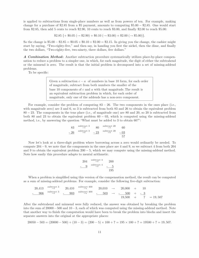
One can extend the Array Model to imagine �× (m× n) as a rectangular 3-dimensional array consistingof � layers of flat arrays of size m×n. This 3-dimensional array can also be viewed as n perpendicular slicesof flat arrays of size �×m. This idea is illustrated in Figure 5 for � = 2, m = 3, and n = 4.

12

Figure 5: The Associative Rule for Multiplication

2 x (3 x 4) (2 x 3) x 4

The Associative Rule for Multiplication is less obvious than the Associative Rule for Addition. Indeed,writing both sides of the property for almost any triple of numbers produces an equation that takes somethought to verify. For example, the product of n = 5, m = 6 and � = 7 can be computed as (5×6)×7 = 30×7or as 5 × (6 × 7) = 5 × 42. Thus, the Associative Rule asserts that 30 × 7 = 5 × 42. While this equationis certainly true, if we did not know where it came from, we probably would have to compute both sides tocheck it.

Note that the Associative Rule for Multiplication may be applied successively to products of more thanthree factors. For instance,

by the associative rule with

2× (3× (4× 5)) = 2× ((3× 4)× 5) � = 3, m = 4, and n = 5= (2× (3× 4))× 5) � = 2, m = 3× 4, and n = 5= ((2× 3)× 4)× 5 � = 2, m = 3, and n = 4= (2× 3)× (4× 5) � = 2× 3, m = 3, and n = 4.

Any-Which-Way Rule for Multiplication: Once students have developed facility with the commutativeand associative rules for multiplication, they can start working with the version of the Any-Which-Way Rulefor multiplication:

The Any-Which-Way Rule for Multiplication : Not only can the factors in a product

of several factors be grouped according to any scheme of parentheses, but also pairs

of them can be interchanged in any way one desires.

For example,

(3× 8)× (7× 8) = 3× (8× (7× 8)) by the Associative Rule for Multiplication

= 3× ((8× 7)× 8) by the Associative Rule for Multiplication

= 3× ((7× 8)× 8) by the Commutative Rule for Multiplication

= 3× (7× (8× 8)) by the Associative Rule for Multiplication

= (3× 7)× (8× 8) by the Associative Rule for Multiplication

Thus, in this example, we could just go ahead and interchange the 8 on the left with the 7 on the right. Thisis a special case of the following useful identity: For all numbers a, b, c, and d,

(a× b)× (c× d) = (a× c)× (b× d).

Someone who thinks that the transformations shown above amount to a lot of work to justify the simpleexchange of factors would be right. Note, however, that when the first and last factors are multiplied out,the result is

24× 56 = (3× 8)× (7× 8) = (3× 7)× (8× 8) = 21× 64,

13

and the equality of the leftmost and rightmost products is not immediately obvious. In addition, the Any-Which-Way Rule is useful for mental arithmetic. For instance, a person who finds it difficult to compute(7× 5)× (6× 2) might see that it is much easier to find the product if the 5 and the 2 are grouped togetherto give a factor of 10:

(7× 5)× (6× 2) = (7× 6)× (2× 5) = 42× 10 = 420.

Exponential Notation: Given any positive integers b and n, we define bn to be the number obtained bymultiplying n copies of b together:

bn = b× b× · · · × b︸ ︷︷ ︸

n factors

We also define b0 to equal 1:b0 = 1.

In the expression bn, b is called the base and n the exponent . By the Any-Which-Way Rule for Multipli-cation, all the different ways we could group the b’s as we compute bn would give the same result. Anotherresult of the Any-Which-Way Rule for Multiplication is the Law of Exponents.

The Law of Exponents: For any positive integer b and all nonnegative integers m and n,

bm × bn = bm+n.

For example,

103 × 105 = 103+5 = 108, 27 × 24 = 27+4 = 211, 6325 × 6352 = 6325+52 = 6377.

Besides its utility in computation, the Law of Exponents reveals a beautiful parallel between multiplicationand addition. The Rules of Arithmetic emphasize the fact that both addition and multiplication are governedby essentially the same four basic rules. This suggests that there might be some deep relationship betweenaddition and multiplication. The Law of Exponents is a concrete expression of this relationship.

The Extended Distributive Rule: Recall from section 2A that the Distributive Rule tells us how tomultiply a number times a sum of two numbers:

The Distributive Rule: For any nonnegative integers a, b and c, we have the equation

a× (b + c) = a× b + a× c.

Just as repeated uses of the commutative and associative rules can be combined to produce an any-which-way rule, so repeated uses of the Distributive Rule, combined with the commutative and associative rules,produce the Extended Distributive Rule. To express this rule, we use a standard convention for indicatinga product of two numbers: instead of writing a multiplication symbol between them we simply put thenumbers side by side.

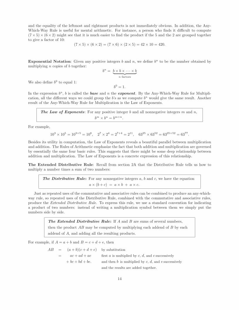
The Extended Distributive Rule: If A and B are sums of several numbers,

then the product AB may be computed by multiplying each addend of B by each

addend of A, and adding all the resulting products.

For example, if A = a + b and B = c + d + e, then

AB = (a + b)(c + d + e) by substitution

= ac + ad + ae first a is multiplied by c, d, and e successively

+ bc + bd + be. and then b is multiplied by c, d, and e successively

and the results are added together.

14

A schematic version of the Extended Distributive Rule for multiplying a sum of 2 numbers by a sum of3 numbers is shown in Figure 6.

ac ad ae

bc bd be

Figure 6: Extended Distributive Rule (Schematic Form)

c d e

a

b

Applying the Rules to Compute Products: The Any-Which-Way rules for addition and multiplicationplus the Extended Distributive Rule, which links multiplication and addition, are the tools we use for multi-plying general numbers in base 10 form. Since each such number is the sum of its single-place components,the Extended Distributive Rule tells us that the product of two of them may be found by multiplying eachsingle-place component of one factor by each single-place component of the other factor, and then addingall the products together. Moreover, the Any-Which-Way Rule for addition says that we have great latitudehow we sum these numbers up. Differences in multiplication algorithms come mainly from choosing differentsummation procedures.

Multiplying Single-Place Numbers: As indicated by the previous paragraph, in order to computeproducts of numbers in base 10 form, it is essential to understand products of single-place numbers. Thesituation is somewhat analogous to that of addition:

Products of Single-Place Numbers: A product of two single-place numbers

equals the product of the digits times the denomination whose magnitude is

equal to the sum of the orders of magnitude of the factors. In other words,

if M = d110m and N = d210n, then

MN = d110m × d210n = d1d2 × 10m+n.

For example,

200× 4000 = (2× 100)× (4× 1000)by writing 200 and 4000 in expanded form

= (2× 4)× (100× 1000)by the Any-Which-Way Rule for Multiplication4

= 8× 100, 000by computing 2 times 4 and 100 times 1000

= 800, 000by converting from expanded form.

15

Another way to express the computation uses exponential notation and the Law of Exponents:

200× 4000 = (2× 102)× (4× 103)by writing 200 and 4000 in expanded form with exponents

= (2× 4)× (102 × 103)by the Any-Which-Way Rule for Multiplication

= 8× 105

by computing 2 times 4 and using the Law of Exponents

= 800, 000by converting from expanded form.

Observe that when two single-place numbers are multiplied, if the product of the digits is less than 10,the result is another single-place number whose magnitude is the sum of the magnitudes of the factors:

30× 200 = 6, 000 = 6× 1000.

If the product of the digits is a multiple of 10, the result is a single-place number whose magnitude is onemore than the sum of the magnitudes of the factors:

60× 500 = 30× 1000 = 30, 000 = 3× 10, 000.

And if the product of the digits is greater than 10 but not divisible by 10, a sum of two single-place numbersis obtained, the larger of which has magnitude that is one more than the sum of the magnitudes of thefactors:

30× 700 = 21, 000 = 20, 000 + 1, 000 = 2× 10, 000 + 1, 000.

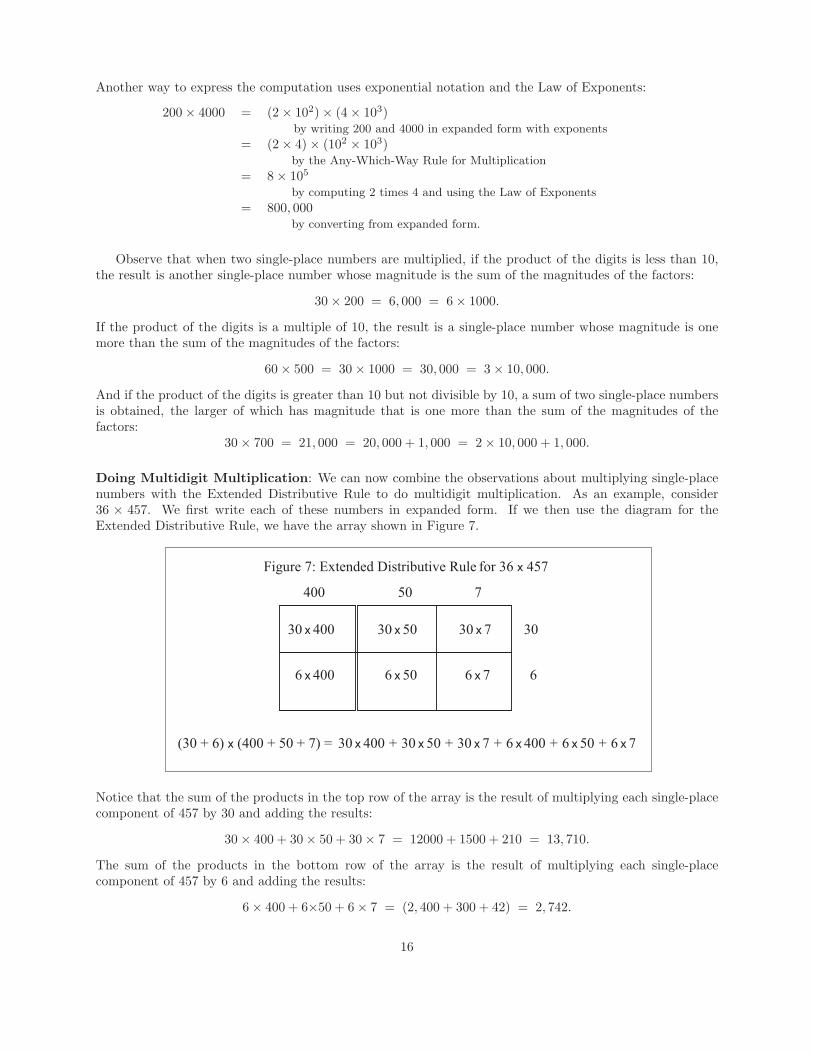
Doing Multidigit Multiplication: We can now combine the observations about multiplying single-placenumbers with the Extended Distributive Rule to do multidigit multiplication. As an example, consider36 × 457. We first write each of these numbers in expanded form. If we then use the diagram for theExtended Distributive Rule, we have the array shown in Figure 7.

400 50 7

(30 + 6) x (400 + 50 + 7) = 30 x 400 + 30 x 50 + 30 x 7 + 6 x 400 + 6 x 50 + 6 x 7

30 x 400 30 x 50 30 x 7

6 x 400 6 x 50 6 x 7

Figure 7: Extended Distributive Rule for 36 x 457

30

6

Notice that the sum of the products in the top row of the array is the result of multiplying each single-placecomponent of 457 by 30 and adding the results:

30× 400 + 30× 50 + 30× 7 = 12000 + 1500 + 210 = 13, 710.

The sum of the products in the bottom row of the array is the result of multiplying each single-placecomponent of 457 by 6 and adding the results:

6× 400 + 6×50 + 6× 7 = (2, 400 + 300 + 42) = 2, 742.

16

These are exactly the numbers obtained for the partial products in a version of the standard algorithm forcomputing 36× 457:

457× 362, 742

13, 71016, 452

Similarly, if we interchange the order of the factors 36 and 457, we obtain

36× 457

2521, 800

14, 40016, 452

where the partial products in the third, fourth, and fifth rows are the sums of the products in the first,second, and third columns of the array shown in Figure 7. The sum of the products in the first columnis the result of multiplying each single-place component of 36 by 400 and adding the results, the sum ofthe products in the second column is the result of multiplying each single-place component of 36 by 50and adding the result, and the sum of the products in the third column is the result of multiplying eachsingle-place component of 36 by 7 and adding the results:

30× 400 + 6× 400 = 400× 6 + 400× 30 = 14, 40030× 50 + 6× 50 = 50× 6 + 50× 30 = 1, 80030× 7 + 6× 7 = 7× 6 + 7× 30 = 252

Another way to think of this is that each of the partial products results from multiplying one of the single-place components of 457 times the number 36: 7× 36 = 252, 50× 36 = 1, 800, and 400× 36 = 14, 400.

Interpreting the standard multiplication algorithm in terms of the array of products of single-place com-ponents could help students to understand why it doesn’t matter which factor in a product comes first, eventhough the intermediate steps in the calculation are so different.

Alternative Algorithms for Multidigit Multiplication

The Lattice Method: Given our base 10 notation, we have tried to show that the most natural way toadd two numbers is to break each addend into its single-place components, sum up the components of eachmagnitude, and then recombine the results. Neither of the standard algorithms for multiplication, however,uses this approach. However, the idea does form the basis for an multiplication algorithm known as theLattice Method (or the Array Method, or Napier’s Bones). It is a refinement of the observation that if wewrite the products of the components in an array, as shown in Figure 8, then the magnitude of the productsdecreases from left to right along rows and from top to bottom along columns.

14,400 1,800 252

30 x 400 = 12,000 30 x 50 = 1,500 30 x 7 = 210

6 x 400 = 2,400 6 x 50 = 300 6 x 7 = 42

Figure 8: Row and Column Totals for 36 x 457

Row Totals

ColumnGrand TotalTotals

13,710

2,742

16,452

17

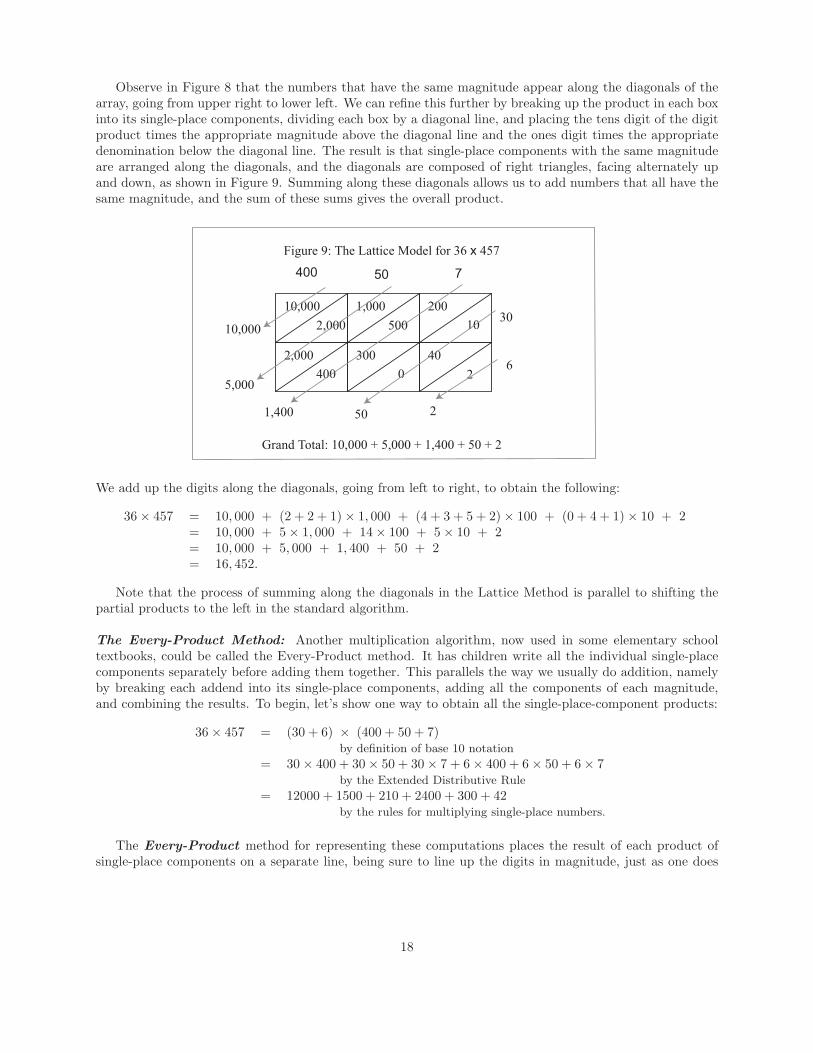
Observe in Figure 8 that the numbers that have the same magnitude appear along the diagonals of thearray, going from upper right to lower left. We can refine this further by breaking up the product in each boxinto its single-place components, dividing each box by a diagonal line, and placing the tens digit of the digitproduct times the appropriate magnitude above the diagonal line and the ones digit times the appropriatedenomination below the diagonal line. The result is that single-place components with the same magnitudeare arranged along the diagonals, and the diagonals are composed of right triangles, facing alternately upand down, as shown in Figure 9. Summing along these diagonals allows us to add numbers that all have thesame magnitude, and the sum of these sums gives the overall product.

10,000 1,000 200

2,000 300 40

2,000 500 10

400 0 2

30

6

Figure 9: The Lattice Model for 36 x 457

400 50 7

10,000

5,000

1,400 50 2

Grand Total: 10,000 + 5,000 + 1,400 + 50 + 2

We add up the digits along the diagonals, going from left to right, to obtain the following:

36× 457 = 10, 000 + (2 + 2 + 1)× 1, 000 + (4 + 3 + 5 + 2)× 100 + (0 + 4 + 1)× 10 + 2= 10, 000 + 5× 1, 000 + 14× 100 + 5× 10 + 2= 10, 000 + 5, 000 + 1, 400 + 50 + 2= 16, 452.

Note that the process of summing along the diagonals in the Lattice Method is parallel to shifting thepartial products to the left in the standard algorithm.

The Every-Product Method: Another multiplication algorithm, now used in some elementary schooltextbooks, could be called the Every-Product method. It has children write all the individual single-placecomponents separately before adding them together. This parallels the way we usually do addition, namelyby breaking each addend into its single-place components, adding all the components of each magnitude,and combining the results. To begin, let’s show one way to obtain all the single-place-component products:

36× 457 = (30 + 6) × (400 + 50 + 7)by definition of base 10 notation

= 30× 400 + 30× 50 + 30× 7 + 6× 400 + 6× 50 + 6× 7by the Extended Distributive Rule

= 12000 + 1500 + 210 + 2400 + 300 + 42by the rules for multiplying single-place numbers.

The Every-Product method for representing these computations places the result of each product ofsingle-place components on a separate line, being sure to line up the digits in magnitude, just as one does

18

for addition. The resulting numbers are then added together:

457× 36

42300

2400210

15001200016452

When this method is used in elementary school, it is essential for children to come to understand that, forexample, the component product 210 comes from multiplying the 3 in the tens place, hence 30, times the7 in the ones place. Similarly, the 12000 comes from multiplying the 3 in the tens place, hence 30, timesthe 4 in the hundreds place, hence 400. Otherwise, teaching this method simply substitutes a less efficientmechanical procedure for a more efficient one.

2D. DivisionThe interactions between ideas about place value and division illuminate both the process of division and

the properties of numbers in base 10 form. In one direction, the idea of division-with-remainder provides asystematic way to find the digits in a number given in base 10 form. In the opposite direction, the effort tofind a method for computing the the nonzero single-place components of a quotient in a division problemleads to another interpretation for long division and the uses of base 10 notation for approximation.

Division-with-Remainder: In its strict sense, division is the inverse operation for multiplication, just assubtraction is the inverse operation for addition. For instance, 6÷ 3 = 2 because 2 × 3 = 6 and 72÷ 9 = 8because 8 × 9 = 72. However, division in this strict sense cannot always be carried out within the set ofnonnegative integers or even within the set of finite decimal numbers. For example, 3÷2 is not a nonnegativeinteger (although it can be represented as the finite decimal 1.5) and 5 ÷ 3 is not only not a nonnegativeinteger, but also its decimal representation, 1.666..., is not even finite.

Thus, for the set of nonnegative integers, instead of simply working with division as the inverse ofmultiplication, we work with division-with-remainder, which is a somewhat more general substitute. Whendivision-with-remainder is carried out, instead of yielding a single number as a result, it yields a pair ofnumbers: a quotient and a remainder.

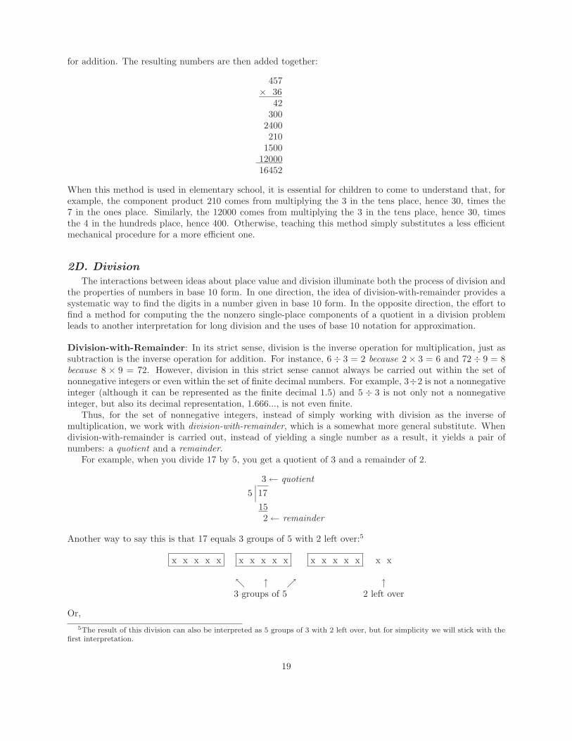
For example, when you divide 17 by 5, you get a quotient of 3 and a remainder of 2.

3← quotient5

∣∣∣17152← remainder

Another way to say this is that 17 equals 3 groups of 5 with 2 left over:5

x x x x x x x x x x x x x x x x x

↖ ↑ ↗ ↑3 groups of 5 2 left over

Or,5The result of this division can also be interpreted as 5 groups of 3 with 2 left over, but for simplicity we will stick with the

first interpretation.

19

17 = 3× 5 + 2.↑ ↑

3 groups of 5 2 left over

The key consideration here is that the number left over (in this case, 2) should be less than the size of thegroups (in this case, 5) because if 5 or more were left over, another group of 5 could be separated off.

One can prove mathematically that this kind of result occurs in general:

Division-with-Remainder Property : When any nonnegative integer n is divided by any

positive integer d, the result is two nonnegative integers: a quotient q and a remainder r,

where r is smaller than d:

n = qd + r and 0 ≤ r < d.

Note that either q or r (or both) could equal zero.

Another way to think of division-with-remainder uses the idea of measurement. For instance, imaginetrying to measure a piece of string of length n centimeters using a ruler of length d centimeters and findingthat it is possible to fit in q copies of the ruler, but that, when you do this, a piece of string of length r isleft over, where r is less than d. Figure 10 shows a picture of that process for n = 17 and d = 5.

Figure 10: 17 = 5 x 3 + 2

A key property of division-with-remainder is that because n = qd + r and r is nonnegative, n is alwaysbetween q times d and (q +1) times d. You can visualize this property in general by thinking of a segment ofthe number line that shows n, some multiples of d, and the remainder r, as shown in Figure 11 Starting atzero and moving q multiples of length d to the right takes you either a little to the left of n (if the remainderr is positive) or directly to n (if the remainder r is zero). But because r < d, if you move to the right of qdby one more block of d units you will go past n. So n has to be between qd and qd+d, which equals (q +1)d.

Figure 11: If n = qd + r, then qd < n < (q + 1)d

Thus, in general:

When division of n by d gives a quotient of q and a remainder of r, thenqd ≤ n < (q + 1)d.

20

Division-with-remainder, both theoretically and practically, depends on the order properties of nonneg-ative integers, which are discussed in section 5. In this section we assume a basic acquaintance with themto give the following formal derivation for the above result: Start with the fact that n = qd + r and theinequality

0 ≤ r < d.

Add qd to all parts of the inequality to obtain

qd ≤ qd + r < qd + d.

Now qd + r = n (by assumption) and qd + d = (q + 1)d (by factoring out d). So

qd ≤ n < (q + 1)d.

For our example of n = 17 and d = 5, we have

3×5 ≤ 3×5 + 2 < 4×5,

or, equivalently,3×5 ≤ 17 < 4×5.

Note that the word quotient is used in two different ways. For instance, we say that the quotient of 11by 4 is 2 with remainder 3, and we also say that the quotient of 11 by 4 is the number 11

4, or 2.75. Because

using exactly the same term to refer to two different things can cause confusion, when we want to be clearthat we are talking about the nonnegative integer q coming from division-with-remainder, we will call it theinteger quotient rather than just the quotient.

Ways to Obtain the Base 10 Form of a Number and Their Interpretations: There are two distinctways to obtain the base 10 form of a number. The first involves repeated division-with-remainder by 10; thesecond, though less well known, is important for understanding long division. The second is also fundamentalfor understanding the approximation properties of base 10 notation (which are discussed in section 5).

Using Successive Division by 10 : Observe that the ones digit of a number is the remainder obtainedwhen the number is divided by 10. For example,

because 6, 407 = 640× 10 + 7, we have that 6, 407÷ 10 is 640 with remainder 7.

Here are the steps showing how the above result was derived:

6, 407 = 6×1000 + 4×100 + 0×10 + 7by converting to expanded form

= 6×100× 10 + 4×10×10 + 0×10 + 7 because multiplying by 10 adds a zero on the right

i.e., by the Law of Exponents: 10n−1×10 = 10n

= (6×100 + 4×10 + 0)×10 + 7by the Extended Distributive Rule

= 640×10 + 7by converting from expanded form.

In general:

When a number in base 10 form is divided by 10, the remainder is the rightmost digit of the number

and the integer quotient is obtained by taking the number and dropping the rightmost digit.

21

Thus, if we go back to the example and continue to divide by 10, we obtain the rest of the digits of thenumber in succession:

640÷ 10 is 64 with remainder 0

64÷ 10 is 6 with remainder 4

6÷ 10 is 0 with remainder 6.

In general:

The digits of a number in base 10 form can be obtained by successive division-with-remainder by 10.

Using Approximation by a Sequence of Single-Place Numbers: A second, seemingly quite different,way to find the composition of a number in base 10 form connects with the idea of approximation andintroduces the principle used to perform long division.

Given any number, we can try to approximate it by sums of single-place numbers. Of course there aremany ways to do this, but one way is an example of what computer scientists call a greedy algorithmbecause at each stage it gets the most it can get at that stage.

Here is the idea of how the greedy algorithm works in this case: Suppose you are given a collection ofspecial numbers, and you want to express an arbitrary number as a sum of the special numbers. For instance,imagine that you want to order a certain number of items from a factory. However, the factory only sellsitems in full boxes, and it only produces boxes of certain sizes. Thus a procedure is needed to decide whichboxes to give you. A greedy algorithm to approximate your order would work as follows: It would first giveyou the largest possible box: that is, the box containing the largest number of items less than or equal tothe number you ordered. Then it would subtract the number of items in that box from the number in yourorder and give you the largest possible box for the remaining items in your order. It would continue thisprocess as long as possible, each time giving you the largest size box for the remaining unboxed items inyour order until either it fills your order completely or there are no available package sizes containing thenumber that remain in your order or fewer than that number.

A wonderful aspect of the base 10 number system is that if the collection of box sizes is the collection ofall the single-place numbers, then the greedy algorithm will always fill your order completely, and it will doso in a way that produces the nonzero single-place components for the number of items in your order. Hereis a description of the algorithm:

Approximation Algorithm: Finding the Nonzero Single-place Components of a Number

Step 1 : Find the largest single-place number that is less than or equal to the given number.

Step 2 : Subtract the number obtained in Step 1 from the given number; the result is the error term .

Step 3 : If the error term is greater than 0, go back to Step 1 using the error term in place of thegiven number.

If the error term is 0, stop: the single-place numbers obtained from the repeated steps ofthe algorithm are the nonzero single-place components of the original number; their sumis the original number.

As an example, suppose your order consists of 6,407 items. Since

6, 000 ≤ 6, 407 < 7, 000,

the greedy algorithm first gives you a box with 6, 000 items. Then it calculates the number remaining (thefirst “error term”) and finds it to be 6, 407− 6, 000 = 407. So, in the next step, since

400 ≤ 407 < 500,

22

the algorithm gives you a box with 400 items. Then it calculates the number remaining (the second “errorterm”) and finds it to be 407− 400 = 7. So, in the next step, since

7 ≤ 7 < 8,

the algorithm gives you a box with 7 items, which completes your order exactly. Observe that the successivebox sizes are precisely the nonzero single-place components of the number of items in your order:

6, 407 = 7, 000 + 400 + 7.

The following property of single-place numbers is the reason that the Approximation Algorithm producesthe desired result. More precisely, it is the fundamental reason that the sum of single-place numbers producedby the Approximation Algorithm contains at most one term of any given order of magnitude.

Key Property of Single-Place Numbers: If one starts with any nonzero single-placenumber and adds the denomination with the same order of magnitude as the number, oneobtains the next larger single-place number.

For instance, if one starts with the number 6,000 in the example above and adds the denomination 1,000, oneobtains 7,000, which is the next larger number after 6,000 that is a product of a digit times a denomination.Similarly, if one starts with 400 and adds the denomination 100, one obtains 500, which is the next largersingle-place number after 400.

In general, when the digit of the single-place number is 1 through 8 and one adds the denomination withthe same order of magnitude, one only needs to increase the digit by 1 to obtain the next larger single-placenumber. (For instance, 60 + 10 = 70. However, when the digit of the single-place number is 9, the nextlarger single-place number is obtained by replacing the 9 by a 10. For example, if the single-place numberis 9,000, the number 10,000 is the next larger single-place number. Note, however, that the Key Propertyof Single-Place Numbers holds in this case also because 1, 000 is the denomination with the same order ofmagnitude as 9, 000 and 9, 000 + 1, 000 = 10, 000.

We now use the Key Property of Single-Place Numbers to give a formal proof of the fact that the greedyalgorithm produces the nonzero single-place components for any number in base 10 form. Let n be anynonnegative integer, and let c be the largest of its single-place components. By the Key Property of Single-Place Numbers, the next larger single-place number is c + m, where m is the denomination with the sameorder of magnitude as c. Since c is chosen to be as large as possible, we know that

c ≤ n < c + m.

So, by subtracting c from all three numbers, we have

0 ≤ n− c < m.

Now the next stage of the approximation process is to approximate the remainder n− c by its largest single-place component, and since n− c < m, the number obtained in this next stage will have a smaller order ofmagnitude than m. This argument shows that when the algorithm is finally complete, the final sum will bethe original number and will have at most one term with any given order of magnitude.

An interesting observation comes out of this way of thinking: If n is a nonnegative integer, c its largestsingle-place component, and r = n− c, then

c > r.

Add c to both sides of this inequality to obtain

2c > c + r = n.

23

Then dividing by 2 givesc >

n

2.

We may state this result in words:

For any nonnegative integer n, the largest single-place component of naccounts for more than half of n.

For example, when n = 199, then the largest single-place component of n is c = 100, half of n isn

2=

1992

=99.5, and 100 > 99.5. In general, however, the largest single-place component of a number is much largerthan half the number. For example, the largest single-place component of 985 is 900, which is much largerthan half of 985. This topic is discussed in greater detail in section 5.

Approximation and Long Division: In this section we show how the ideas we have been developingunderlie the process of long division. The basis for the discussion is that in division-with-remainder of nby d, the integer quotient is the largest nonnegative integer q such that dq ≤ n. Because the search for aninteger satisfying this kind of property formed the basis for each of the steps in the greedy algorithm to findthe base 10 expansion of a number, we can adapt the explanation for the success of the greedy algorithm toexplain why the long-division process produces the correct answer. In fact, the justification for what we callthe Basic Fact of Long Division uses the same Key Property of Single-Place Numbers that guaranteed thatthe greedy algorithm would produce the nonzero single-place components of a number.

Basic Fact of Long Division : Suppose that q is the integer quotient of n divided by d. In otherwords, suppose that n = qd + r, where 0 ≤ r < d. Then the largest single-place component of q

is the largest single-place number s such that sd ≤ n.

Before discussing the justification for the Basic Fact of Long Division, we examine how it is used in thelong-division process. In general, the problem of long division is to find the base 10 representations for thenonnegative integer quotient q and the remainder r of the division of one nonnegative integer n by a positiveinteger d. In other words, the problem is to find the base 10 representations for nonnegative integers q and rsuch that n = qd+r and 0 ≤ r < d. By definition of base 10 notation, this is equivalent to finding (and thenadding up) all the single-place components of q for the division of n by d and also to finding the remainderfor this division.

Now the Basic Fact of Long Division says that the largest single-place component of q is the largestsingle-place number s with sd ≤ n. To find the second largest single-place component of q, which we willcall s1, we subtract sd from n to obtain the difference n1 = n − sd and repeat the process with n1 inplace of n. Then the Basic Fact of Long Division tells us that s1 is the largest single-place number withs1d ≤ n1. Continuing in this way is exactly what one does in long division, until eventually one obtains adifference that is less than the divisor d. This turns out to be the remainder r, and the sum of the single-placecomponents obtained in the individual steps is the integer quotient q. We summarize this procedure in thefollowing algorithm:

24

Algorithm for the Long Division of n by d

Step 1 : Find the largest single-place number s whose product with d is less than or equal to n.

Step 2 : Subtract s from n; call the result the error term .

Step 3 : If the error term is greater than or equal to d, go back to Step 1 using the error termin place of n.

If the error term is less than d, then it is the remainder of the division of n by dand the sum of the single-place numbers obtained from the repetitions of Step 1is the integer quotient of the division.

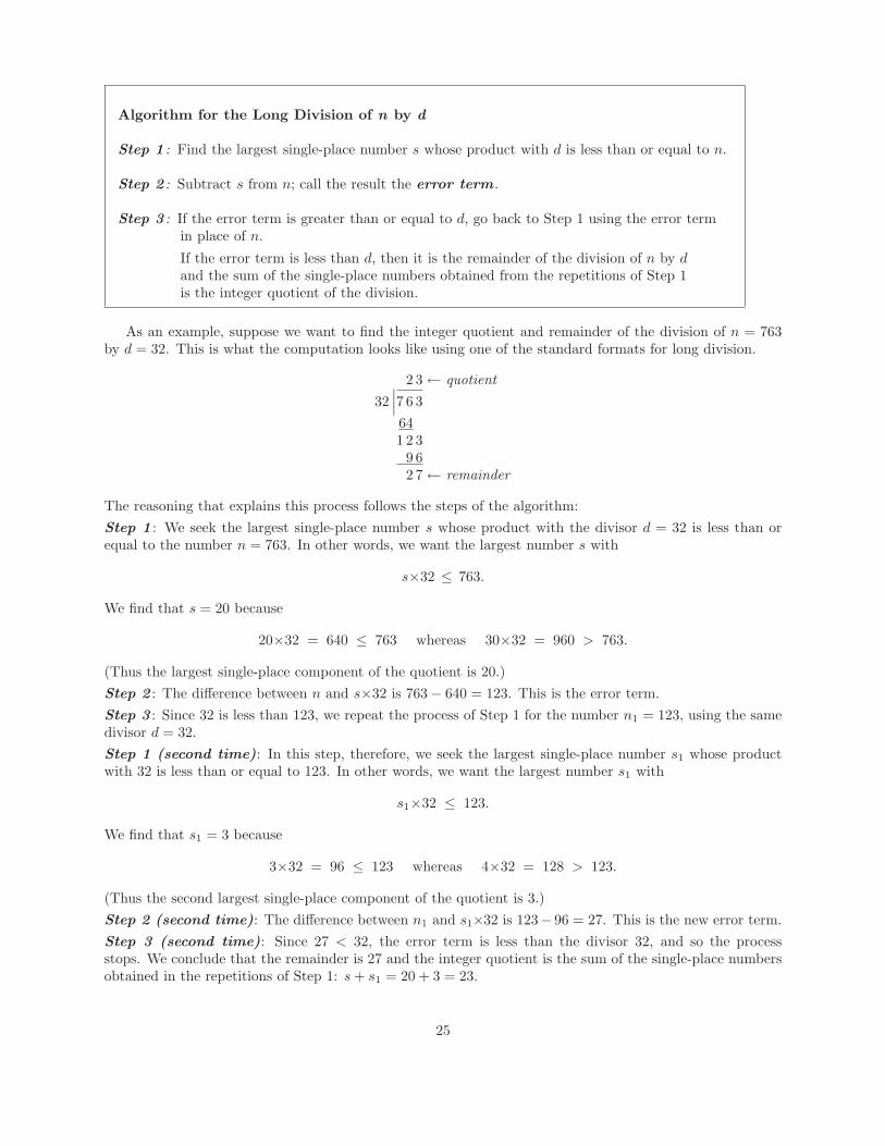
As an example, suppose we want to find the integer quotient and remainder of the division of n = 763by d = 32. This is what the computation looks like using one of the standard formats for long division.

2 3← quotient32

∣∣∣7 6 3641 2 3

9 62 7← remainder

The reasoning that explains this process follows the steps of the algorithm:Step 1 : We seek the largest single-place number s whose product with the divisor d = 32 is less than orequal to the number n = 763. In other words, we want the largest number s with

s×32 ≤ 763.

We find that s = 20 because

20×32 = 640 ≤ 763 whereas 30×32 = 960 > 763.

(Thus the largest single-place component of the quotient is 20.)Step 2 : The difference between n and s×32 is 763− 640 = 123. This is the error term.Step 3 : Since 32 is less than 123, we repeat the process of Step 1 for the number n1 = 123, using the samedivisor d = 32.

Step 1 (second time): In this step, therefore, we seek the largest single-place number s1 whose productwith 32 is less than or equal to 123. In other words, we want the largest number s1 with

s1×32 ≤ 123.

We find that s1 = 3 because

3×32 = 96 ≤ 123 whereas 4×32 = 128 > 123.

(Thus the second largest single-place component of the quotient is 3.)Step 2 (second time): The difference between n1 and s1×32 is 123− 96 = 27. This is the new error term.Step 3 (second time): Since 27 < 32, the error term is less than the divisor 32, and so the processstops. We conclude that the remainder is 27 and the integer quotient is the sum of the single-place numbersobtained in the repetitions of Step 1: s + s1 = 20 + 3 = 23.

25

Justification for the Basic Fact of Long Division : The justification for the Basic Fact of Long Divisionparallels the discussion for the approximation interpretation of the base 10 expansion. Suppose s is chosento be the largest single-place number such that sd ≤ n and suppose m is the denomination with the sameorder of magnitude as s. Then, by the Key Property of Single-Place Numbers, the next larger single-placenumber after s is s + m, and thus

n < (s + m)d.

In addition, because qd ≤ qd + r and qd + r = n, we also have that

qd ≤ n.

We may put these two inequalities together to obtain

qd ≤ n < (s + m)d.

Dividing by d yieldsq < s + m.

Hence because s + m is the next larger single-place number after s and because s + m is greater than q,we conclude that s is the largest single-place number less than or equal to q. Thus, by the approximationinterpretation for the base 10 expansion, s is the largest single-place component of q. This is exactly theclaim of the Basic Fact of Long Division.

Summary : The Basic Fact of Long Division makes long division a practical algorithm although executingit does require fluency with multiplication and subtraction. It also demands some skill in estimation, butwhat is needed in practice ordinarily comes down to division of two- or three- digit numbers by two-digitnumbers. As a multi-step procedure, it can seem somewhat lengthy, but a solid understanding of theunderlying principle can give students confidence in the process. Note also that because long division startsout by finding the largest digits of the result, rather than the smallest digits as with the algorithms for theother three operations, one can stop after carrying out the steps to a point where one has an answer that issufficiently accurate for one’s purposes. Section 5 on approximation deepens and extends the ideas in thissection.

3. Decimal Fractions

Part of the genius of the place-value system for representing numbers is that the same strategy used toexpress and compute with nonnegative integers extends with only minor modifications to a much broaderclass of numbers that involve fractional quantities.

Basic Properties of Fractions: In this section we assume basic familiarity with fractions and theirproperties. We will use the word fraction to refer to a symbol a

b, where a and b are nonnegative integers

and b is not zero, and we call a the numerator and b the denominator of a

b. The symbol a

brepresents a

number, namely the result of dividing a by b. We make special note of two properties of fractions.

Rule for Multiplying Fractions: The product of two fractions is the fraction whose numerator is theproduct of the numerators and whose denominator is the product of the denominators. In symbols: Givenfractions

a

band

c

d,

a

b× c

d=

ac

bd.

In particular, if a and b are nonnegative integers and b = 0, then

a× 1b

=a× 11× b

=a

1× 1

b=

a

b.

26

Equivalent Fractions Property: If k is any positive integer, then ka

kbrepresents the same number as does

a

bbecause ka

kb= k

k× a

b= 1 × a

b= a

b. Thus,

a

b=

ka

kb.

Definition of Decimal Fraction: A decimal fraction is any fraction whose numerator is anonnegative integer and whose denominator is a power of 10. In other words,a decimal fraction is any fraction of the form

a

10mwhere a and m are nonnegative integers.

Recall that 100 = 1. Thus every nonnegative integer can be written as a decimal fraction. For example,1 = 1

100and 3 = 3

100. However, there are many fractions that are not decimal fractions. For instance, 1

3cannot be written as a single nonnegative integer divided by a power of 10.6 It follows that the set of decimalfractions is not closed under division because while both 1 and 3 are decimal fractions, their quotient is not.

Given that not all fractions are decimal fractions and given that not all arithmetic can be performedwithin the set of decimal fractions, why single them out as special? Two features have led to their widespreaduse, and the advent of electronic calculators has made these features increasingly important. The first isthat the computational algorithms developed for numbers in base 10 form extend with almost no change tocomputations with decimal fractions. Since arithmetic with general fractions seems to cause trouble for agreat many people, the relative simplicity of computing with decimal fractions is very attractive.

The second feature is that any real number can be approximated as closely as one wishes by decimalfractions. This is often expressed by saying that the decimal fractions are dense in the set of real numbers.Furthermore, the approximation process is straightforward, in the sense that the same “greedy algorithm,”described in section 2D, that works for nonnegative integers applies to general decimal fractions. Thiscombination of familiar, effective computational methods with the ability to approximate means that onecan do approximate arithmetic to arbitrary accuracy with arbitrary numbers. So, for practical purposes,working with decimal fractions allows us to compute anything we want. In fact, as will be seen in section5, the accuracy of decimal approximations increases rapidly with the number of digits used, so that we canusually get enough accuracy without having to do a great many computations.

Multiplication and Addition with Decimal Fractions, I: Given decimal fractions a

10mand b

10n, we

can multiply them by using the Rule for Multiplying Fractions, the Any-Which-Way Rule for multiplicationof integers, and the Law of Exponents. The result is as follows:

Formula for Multiplying Decimal Fractions: Given decimal fractions a

10mand b

10n,

a

10m× b

10n=

a× b

10m × 10n=

ab

10m+n.

To add two decimal fractions a

10mand b

10n, as for any two fractions, we need to put them over a common

denominator. However this is easier for decimal fractions than for general fractions because one of the powers10m or 10n has to divide the other. To be precise, suppose that m ≤ n. Then by the Law of Exponents,10n = 10m × 10n−m. Thus

a

10m=

a× 10n−m

10m × 10n−m=

a× 10n−m

10n.

6Suppose that1

3=

a

10mfor some nonnegative integers a and m. Multiplying both sides by 3×10m gives 10m = 3a,

and since 3 is a factor of the righthand side of the equation, it must also be a factor of the lefthand side. But this

cannot be the case because 3 is not a factor of 10. So the equation1

3=

a

10mcannot ever be true, no matter what

positive integers we might try to substitute for a and m.

27

The following formula follows immediately:

Formula for Adding Decimal Fractions: Given decimal fractions a

10mand b

10nwith m ≤ n,

a

10m+

b

10n=

a× 10n−m

10n+

b

10n=

a× 10n−m + b

10n.

Since we know how to do the integer arithmetic to compute the numerators of the final expressions in theformulas for multiplying and adding decimal fractions, these formulas provide practical and easily appliedprocedures for doing arithmetic. As an example of how they work, consider multiplying 638

10and 47

100:

63810× 47

100=

638× 4710× 100

=29, 9861000

.

In addition, because63810

=638× 1010× 10

=6380100

,

we have that63810

+47100

=6380100

+47100

=6380 + 47

100=

6427100

.

Decimal Expansions: As stated above, the formulas for multiplying and adding decimal fractions do notindicate why these fractions have special importance. In fact, we could write similar formulas for fractionshaving denominators that are not powers of 10. The reason for singling out denominators which are powersof 10 is that we can extend the notion of single-place number to include digits divided by powers of 10 aswell as digits multiplied by powers of 10. With this extension, every decimal fraction can be expressed as asum of single-place numbers. For example, the numbers used in the preceding calculations can be writtenas follows:

63810

=600 + 30 + 8

10=

60010

+3010

+810

= 60 + 3 +810

and47100

=40 + 7100

=40100

+7

100=

410

+7

100.

This extension of our base 10 notation is further strengthened if we use the standard notation for negativeexponents. By definition

b−n =1bn

for all positive numbers b and n.

With this definition the Law of Exponents is valid for all integer exponents:Law of Exponents: For all integers m, n, and b with b > 0,

bm × bn = bm+n.

By using negative exponents we may rewrite the previous examples as

63810

= 6×101 + 3×100 + 8×10−1

and47100

= 4×10−1 + 7×10−2.

28

In general, the base 10 system for writing nonnegative integers is based on the denominations

. . . d6 d5 d4 d3 d2 d1 d0

. . . 1,000,000 100,000 10,000 1000 100 10 1

. . . 106 105 104 103 102 101 100

Extending the system of denominations to include powers with negative exponents gives the followingresult:

. . . d2 d1 d0 d−1 d−2 d−3 . . .

. . . 100 10 1110

1100

11000

. . .

. . . 102 101 100 1101

1102

1103

. . .

. . . 102 101 100 10−1 10−2 10−3 . . .

Thus we may extend the definition of single-place number to be the product of a digit times anypower of 10 – positive, negative, or zero, and so we now regard all of the following as single-place numbers:

4× 102, 0× 101, 2× 100, 5× 10−1, 2× 10−2, 3× 10−3.

When n is negative, we may call a×10n a fractional single-place number . The definition of order ofmagnitude of a single-place number remains the same: it is the exponent of the power of 10 used to expressthe number. Thus, for example, 3

100has order of magnitude −2 because

2100

= 2× 1100

= 2× 1102

= 2× 10−2.

More generally, if d is an integer from 1 to 9, then the order of magnitude of d

10nis −n.

Since every nonnegative integer is a sum of single-place components, knowing the corresponding digit foreach power of 10 is enough to determine a number’s value. This is the information the base 10 notation givesus: it writes the sequence of digits, from right to left, beginning with the digit for 1 = 100. The location ofa digit in this sequence tells us the power of 10 by which it should be multiplied.

We now see that decimal fractions have a similar expansion: they can be written as sums whose termsare digits times powers of 10, possibly using negative as well as positive powers. Of course, if we only needto express nonnegative integers in base 10 notation, we do not have to include a decimal point because thepower of 10 by which each digit is to be multiplied is clear: the rightmost digit of the number is to bemultiplied by 1, the next digit to the left by 10, the one to the left of that by 102 = 100, and so forth.

A given decimal fraction is determined by the digits which multiply the powers of 10, noting that thesedigits are only nonzero for finitely many powers. The digits naturally make a sequence, with the position of adigit in the sequence determined by which power of 10 it multiplies. When we were dealing with integers, thissequence had a natural start, namely the ones place (order of magnitude zero), and progressed indefinitelyfar to the left. With fractions, however, the sequence can extend arbitrarily far in both directions. So, toknow which digits go with which powers of 10, we have to show explicitly where to find the location of thedigit with magnitude zero (the ones place).

The standard way to do this is to place a mark, the decimal point, between the digit for 100 = 1 andthe digit for 10−1 = 1

10. The digits to the left of the decimal point are multiplied by nonnegative powers

of 10, and the digits to its right are multiplied by successive negative powers of 10. For the numbers in theprevious example, we have

63810

= 60 + 3 +810

= 63.8, and47100

=410

+7

100= .47.

29

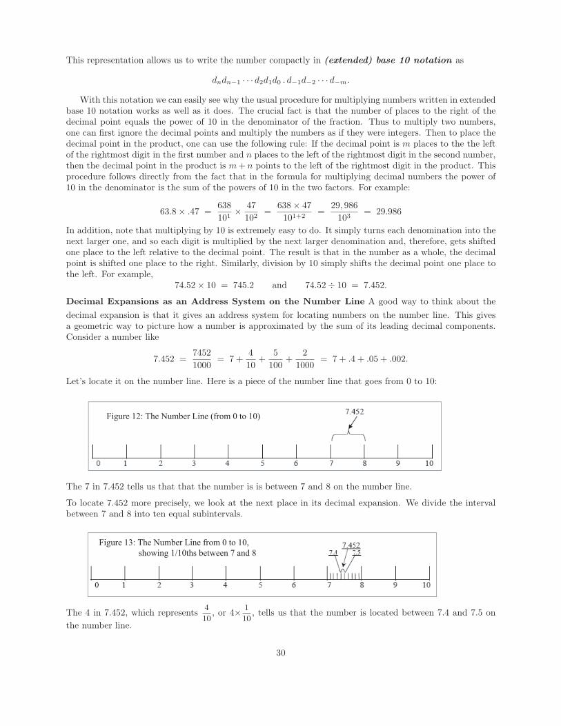
This representation allows us to write the number compactly in (extended) base 10 notation as

dndn−1 · · · d2d1d0 . d−1d−2 · · · d−m.

With this notation we can easily see why the usual procedure for multiplying numbers written in extendedbase 10 notation works as well as it does. The crucial fact is that the number of places to the right of thedecimal point equals the power of 10 in the denominator of the fraction. Thus to multiply two numbers,one can first ignore the decimal points and multiply the numbers as if they were integers. Then to place thedecimal point in the product, one can use the following rule: If the decimal point is m places to the the leftof the rightmost digit in the first number and n places to the left of the rightmost digit in the second number,then the decimal point in the product is m + n points to the left of the rightmost digit in the product. Thisprocedure follows directly from the fact that in the formula for multiplying decimal numbers the power of10 in the denominator is the sum of the powers of 10 in the two factors. For example:

63.8× .47 =638101× 47

102=

638× 47101+2

=29, 986

103= 29.986

In addition, note that multiplying by 10 is extremely easy to do. It simply turns each denomination into thenext larger one, and so each digit is multiplied by the next larger denomination and, therefore, gets shiftedone place to the left relative to the decimal point. The result is that in the number as a whole, the decimalpoint is shifted one place to the right. Similarly, division by 10 simply shifts the decimal point one place tothe left. For example,

74.52× 10 = 745.2 and 74.52÷ 10 = 7.452.

Decimal Expansions as an Address System on the Number Line A good way to think about thedecimal expansion is that it gives an address system for locating numbers on the number line. This givesa geometric way to picture how a number is approximated by the sum of its leading decimal components.Consider a number like

7.452 =74521000

= 7 +410

+5

100+

21000

= 7 + .4 + .05 + .002.

Let’s locate it on the number line. Here is a piece of the number line that goes from 0 to 10:

Figure 12: The Number Line (from 0 to 10)

The 7 in 7.452 tells us that that the number is is between 7 and 8 on the number line.

To locate 7.452 more precisely, we look at the next place in its decimal expansion. We divide the intervalbetween 7 and 8 into ten equal subintervals.

Figure 13: The Number Line from 0 to 10, showing 1/10ths between 7 and 8

The 4 in 7.452, which represents 4

10, or 4× 1

10, tells us that the number is located between 7.4 and 7.5 on

the number line.

30

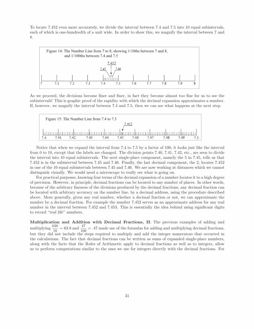
To locate 7.452 even more accurately, we divide the interval between 7.4 and 7.5 into 10 equal subintervals,each of which is one-hundredth of a unit wide. In order to show this, we magnify the interval between 7 and8.

Figure 14: The Number Line from 7 to 8, showing 1/10ths between 7 and 8, and 1/100ths between 7.4 and 7.5

As we proceed, the divisions become finer and finer, in fact they become almost too fine for us to see thesubintervals! This is graphic proof of the rapidity with which the decimal expansion approximates a number.If, however, we magnify the interval between 7.4 and 7.5, then we can see what happens at the next step.

Figure 15: The Number Line from 7.4 to 7.5

Notice that when we expand the interval from 7.4 to 7.5 by a factor of 100, it looks just like the intervalfrom 0 to 10, except that the labels are changed. The division points 7.40, 7.41, 7.42, etc., are seen to dividethe interval into 10 equal subintervals. The next single-place component, namely the 5 in 7.45, tells us that7.452 is in the subinterval between 7.45 and 7.46. Finally, the last decimal component, the 2, locates 7.452in one of the 10 equal subintervals between 7.45 and 7.46. We are now working at distances which we cannotdistinguish visually. We would need a microscope to really see what is going on.

For practical purposes, knowing four terms of the decimal expansion of a number locates it to a high degreeof precision. However, in principle, decimal fractions can be located to any number of places. In other words,because of the arbitrary fineness of the divisions produced by the decimal fractions, any decimal fraction canbe located with arbitrary accuracy on the number line, by a decimal address, using the procedure describedabove. More generally, given any real number, whether a decimal fraction or not, we can approximate thenumber by a decimal fraction. For example the number 7.452 serves as an approximate address for any realnumber in the interval between 7.452 and 7.453. This is essentially the idea behind using significant digitsto record “real life” numbers.

Multiplication and Addition with Decimal Fractions, II: The previous examples of adding andmultiplying 638

10= 63.8 and 47

100= .47 made use of the formulas for adding and multiplying decimal fractions,

but they did not include the steps required to multiply and add the integer numerators that occurred inthe calculations. The fact that decimal fractions can be written as sums of expanded single-place numbers,along with the facts that the Rules of Arithmetic apply to decimal fractions as well as to integers, allowus to perform computations similar to the ones we use for integers directly with the decimal fractions. For

31

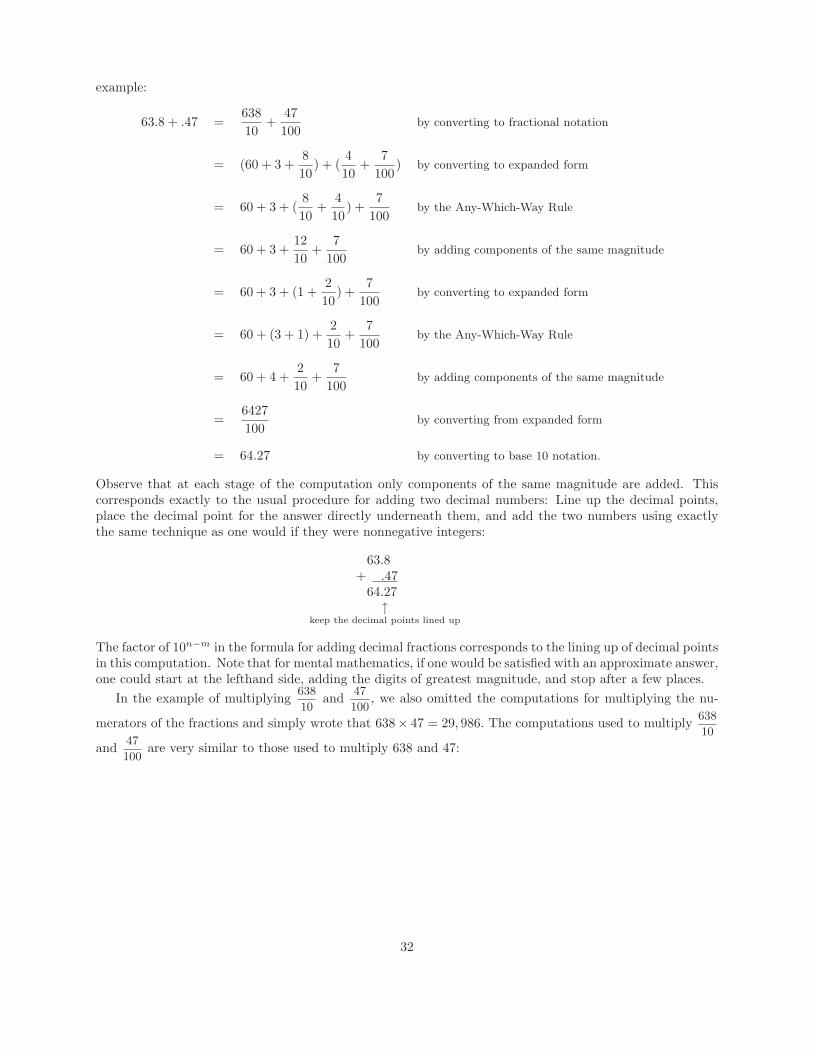
example:

63.8 + .47 =63810

+47100

by converting to fractional notation

= (60 + 3 +810

) + (410

+7

100) by converting to expanded form

= 60 + 3 + (810

+410

) +7

100by the Any-Which-Way Rule

= 60 + 3 +1210

+7

100by adding components of the same magnitude

= 60 + 3 + (1 +210

) +7

100by converting to expanded form

= 60 + (3 + 1) +210

+7

100by the Any-Which-Way Rule

= 60 + 4 +210

+7

100by adding components of the same magnitude

=6427100

by converting from expanded form

= 64.27 by converting to base 10 notation.

Observe that at each stage of the computation only components of the same magnitude are added. Thiscorresponds exactly to the usual procedure for adding two decimal numbers: Line up the decimal points,place the decimal point for the answer directly underneath them, and add the two numbers using exactlythe same technique as one would if they were nonnegative integers:

63.8+ .47

64.27↑

keep the decimal points lined up

The factor of 10n−m in the formula for adding decimal fractions corresponds to the lining up of decimal pointsin this computation. Note that for mental mathematics, if one would be satisfied with an approximate answer,one could start at the lefthand side, adding the digits of greatest magnitude, and stop after a few places.

In the example of multiplying 638

10and 47

100, we also omitted the computations for multiplying the nu-

merators of the fractions and simply wrote that 638× 47 = 29, 986. The computations used to multiply 638

10

and 47

100are very similar to those used to multiply 638 and 47:

32

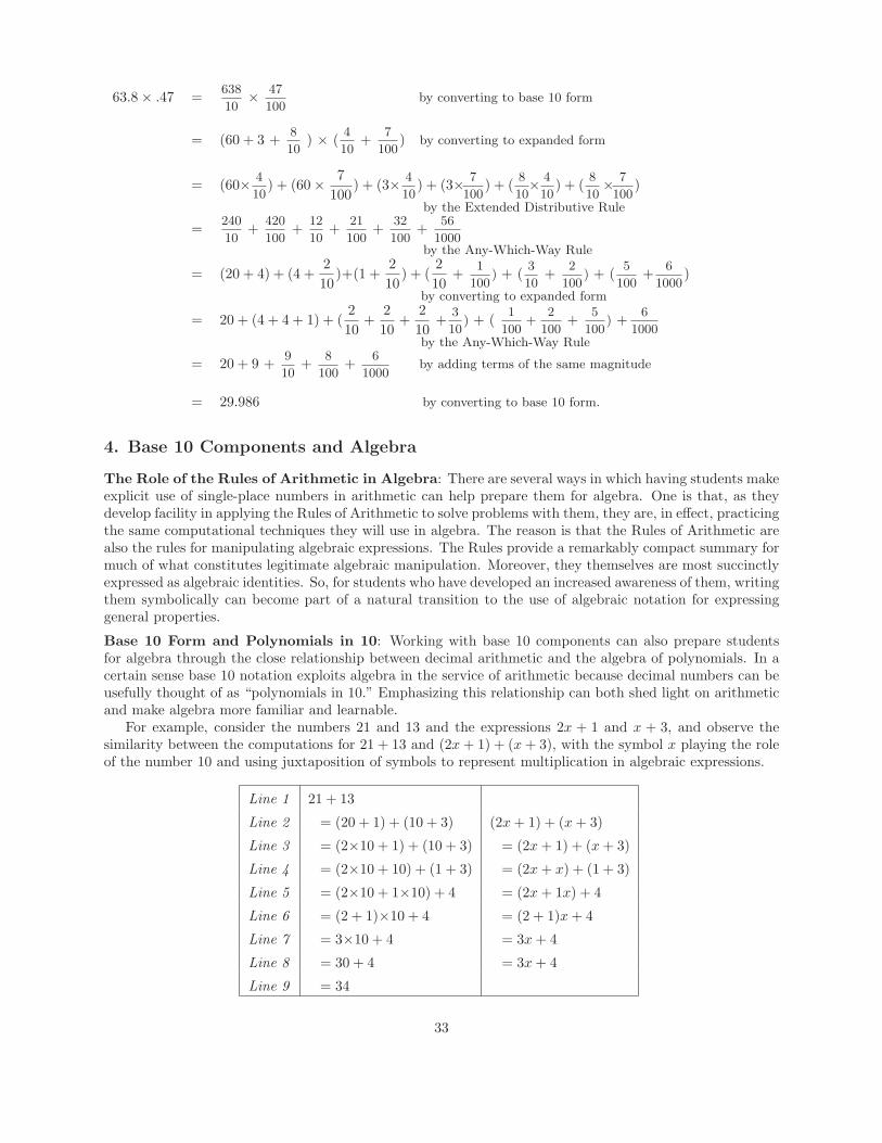
63.8× .47 = 638

10× 47

100by converting to base 10 form

= (60 + 3 + 8

10) × ( 4

10+ 7

100) by converting to expanded form

= (60× 4

10) + (60× 7

100) + (3× 4

10) + (3× 7

100) + ( 8

10× 4

10) + ( 8

10× 7

100)

by the Extended Distributive Rule

= 240

10+ 420

100+ 12

10+ 21

100+ 32

100+ 56

1000by the Any-Which-Way Rule

= (20 + 4) + (4 +210

)+(1 +210

) + (210

+ 1

100) + ( 3

10+ 2

100) + ( 5

100+ 6

1000)

by converting to expanded form

= 20 + (4 + 4 + 1) + (210

+210

+210

+ 3

10) + ( 1

100+

2

100+ 5

100) + 6

1000by the Any-Which-Way Rule

= 20 + 9 + 9

10+ 8

100+ 6

1000by adding terms of the same magnitude

= 29.986 by converting to base 10 form.

4. Base 10 Components and Algebra

The Role of the Rules of Arithmetic in Algebra: There are several ways in which having students makeexplicit use of single-place numbers in arithmetic can help prepare them for algebra. One is that, as theydevelop facility in applying the Rules of Arithmetic to solve problems with them, they are, in effect, practicingthe same computational techniques they will use in algebra. The reason is that the Rules of Arithmetic arealso the rules for manipulating algebraic expressions. The Rules provide a remarkably compact summary formuch of what constitutes legitimate algebraic manipulation. Moreover, they themselves are most succinctlyexpressed as algebraic identities. So, for students who have developed an increased awareness of them, writingthem symbolically can become part of a natural transition to the use of algebraic notation for expressinggeneral properties.

Base 10 Form and Polynomials in 10: Working with base 10 components can also prepare studentsfor algebra through the close relationship between decimal arithmetic and the algebra of polynomials. In acertain sense base 10 notation exploits algebra in the service of arithmetic because decimal numbers can beusefully thought of as “polynomials in 10.” Emphasizing this relationship can both shed light on arithmeticand make algebra more familiar and learnable.

For example, consider the numbers 21 and 13 and the expressions 2x + 1 and x + 3, and observe thesimilarity between the computations for 21 + 13 and (2x + 1) + (x + 3), with the symbol x playing the roleof the number 10 and using juxtaposition of symbols to represent multiplication in algebraic expressions.

Line 1 21 + 13

Line 2 = (20 + 1) + (10 + 3) (2x + 1) + (x + 3)

Line 3 = (2×10 + 1) + (10 + 3) = (2x + 1) + (x + 3)

Line 4 = (2×10 + 10) + (1 + 3) = (2x + x) + (1 + 3)

Line 5 = (2×10 + 1×10) + 4 = (2x + 1x) + 4

Line 6 = (2 + 1)×10 + 4 = (2 + 1)x + 4

Line 7 = 3×10 + 4 = 3x + 4

Line 8 = 30 + 4 = 3x + 4

Line 9 = 34

33

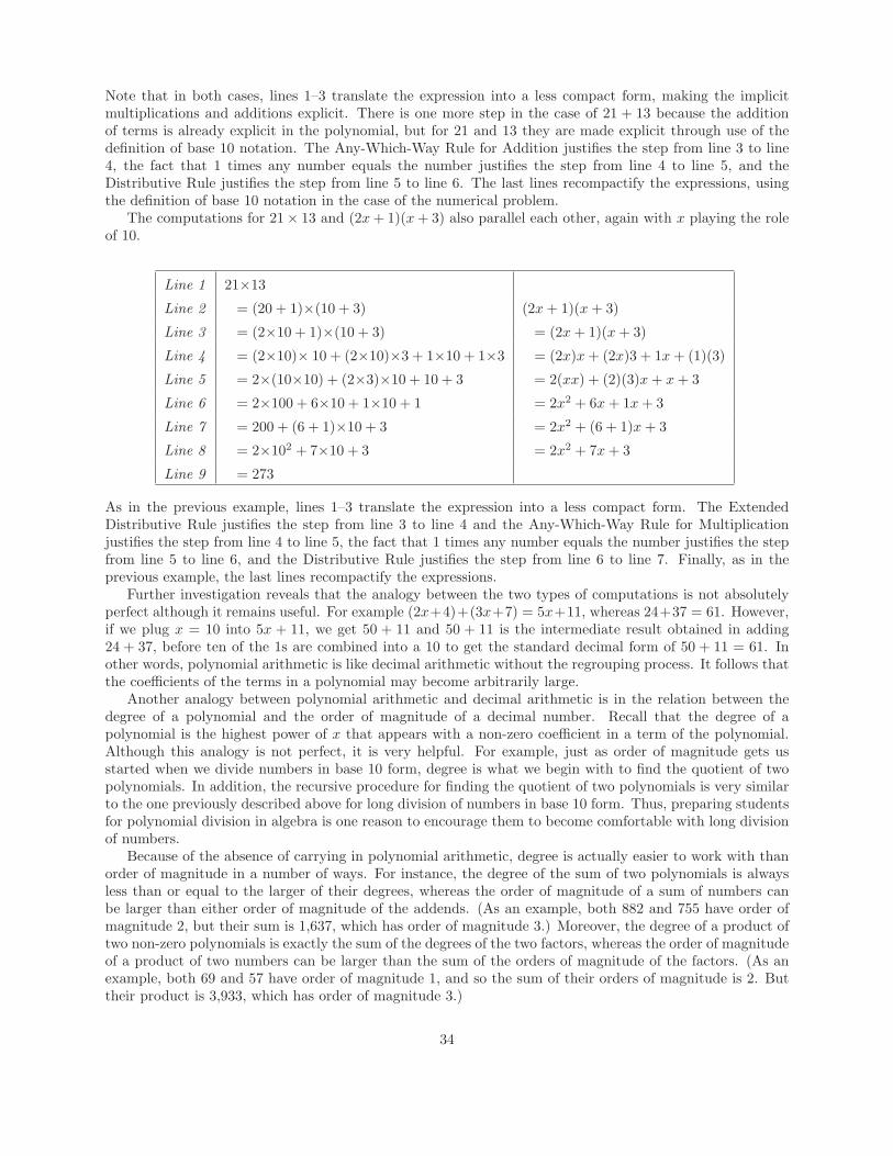
Note that in both cases, lines 1–3 translate the expression into a less compact form, making the implicitmultiplications and additions explicit. There is one more step in the case of 21 + 13 because the additionof terms is already explicit in the polynomial, but for 21 and 13 they are made explicit through use of thedefinition of base 10 notation. The Any-Which-Way Rule for Addition justifies the step from line 3 to line4, the fact that 1 times any number equals the number justifies the step from line 4 to line 5, and theDistributive Rule justifies the step from line 5 to line 6. The last lines recompactify the expressions, usingthe definition of base 10 notation in the case of the numerical problem.

The computations for 21× 13 and (2x + 1)(x + 3) also parallel each other, again with x playing the roleof 10.

Line 1 21×13

Line 2 = (20 + 1)×(10 + 3) (2x + 1)(x + 3)

Line 3 = (2×10 + 1)×(10 + 3) = (2x + 1)(x + 3)

Line 4 = (2×10)× 10 + (2×10)×3 + 1×10 + 1×3 = (2x)x + (2x)3 + 1x + (1)(3)

Line 5 = 2×(10×10) + (2×3)×10 + 10 + 3 = 2(xx) + (2)(3)x + x + 3

Line 6 = 2×100 + 6×10 + 1×10 + 1 = 2x2 + 6x + 1x + 3

Line 7 = 200 + (6 + 1)×10 + 3 = 2x2 + (6 + 1)x + 3

Line 8 = 2×102 + 7×10 + 3 = 2x2 + 7x + 3

Line 9 = 273

As in the previous example, lines 1–3 translate the expression into a less compact form. The ExtendedDistributive Rule justifies the step from line 3 to line 4 and the Any-Which-Way Rule for Multiplicationjustifies the step from line 4 to line 5, the fact that 1 times any number equals the number justifies the stepfrom line 5 to line 6, and the Distributive Rule justifies the step from line 6 to line 7. Finally, as in theprevious example, the last lines recompactify the expressions.

Further investigation reveals that the analogy between the two types of computations is not absolutelyperfect although it remains useful. For example (2x+4)+(3x+7) = 5x+11, whereas 24+37 = 61. However,if we plug x = 10 into 5x + 11, we get 50 + 11 and 50 + 11 is the intermediate result obtained in adding24 + 37, before ten of the 1s are combined into a 10 to get the standard decimal form of 50 + 11 = 61. Inother words, polynomial arithmetic is like decimal arithmetic without the regrouping process. It follows thatthe coefficients of the terms in a polynomial may become arbitrarily large.

Another analogy between polynomial arithmetic and decimal arithmetic is in the relation between thedegree of a polynomial and the order of magnitude of a decimal number. Recall that the degree of apolynomial is the highest power of x that appears with a non-zero coefficient in a term of the polynomial.Although this analogy is not perfect, it is very helpful. For example, just as order of magnitude gets usstarted when we divide numbers in base 10 form, degree is what we begin with to find the quotient of twopolynomials. In addition, the recursive procedure for finding the quotient of two polynomials is very similarto the one previously described above for long division of numbers in base 10 form. Thus, preparing studentsfor polynomial division in algebra is one reason to encourage them to become comfortable with long divisionof numbers.

Because of the absence of carrying in polynomial arithmetic, degree is actually easier to work with thanorder of magnitude in a number of ways. For instance, the degree of the sum of two polynomials is alwaysless than or equal to the larger of their degrees, whereas the order of magnitude of a sum of numbers canbe larger than either order of magnitude of the addends. (As an example, both 882 and 755 have order ofmagnitude 2, but their sum is 1,637, which has order of magnitude 3.) Moreover, the degree of a product oftwo non-zero polynomials is exactly the sum of the degrees of the two factors, whereas the order of magnitudeof a product of two numbers can be larger than the sum of the orders of magnitude of the factors. (As anexample, both 69 and 57 have order of magnitude 1, and so the sum of their orders of magnitude is 2. Buttheir product is 3,933, which has order of magnitude 3.)

34

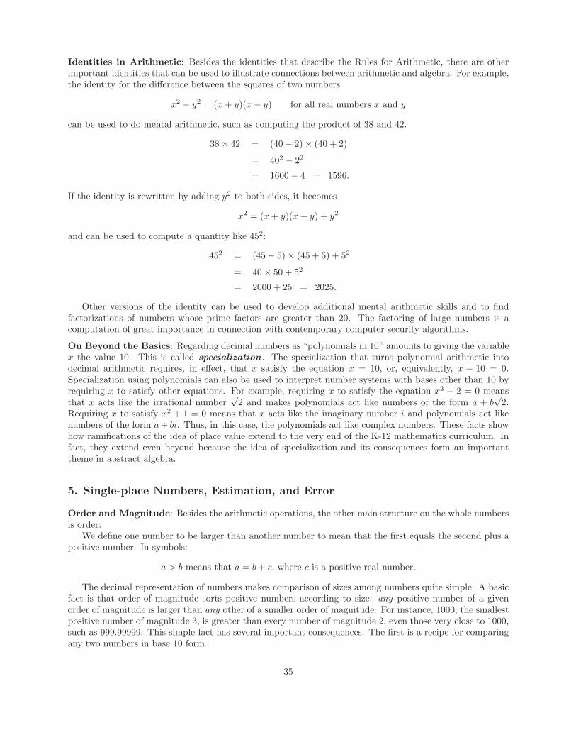
Identities in Arithmetic: Besides the identities that describe the Rules for Arithmetic, there are otherimportant identities that can be used to illustrate connections between arithmetic and algebra. For example,the identity for the difference between the squares of two numbers

x2 − y2 = (x + y)(x− y) for all real numbers x and y

can be used to do mental arithmetic, such as computing the product of 38 and 42.

38× 42 = (40− 2)× (40 + 2)

= 402 − 22

= 1600− 4 = 1596.

If the identity is rewritten by adding y2 to both sides, it becomes

x2 = (x + y)(x− y) + y2

and can be used to compute a quantity like 452:

452 = (45− 5)× (45 + 5) + 52

= 40× 50 + 52

= 2000 + 25 = 2025.

Other versions of the identity can be used to develop additional mental arithmetic skills and to findfactorizations of numbers whose prime factors are greater than 20. The factoring of large numbers is acomputation of great importance in connection with contemporary computer security algorithms.

On Beyond the Basics: Regarding decimal numbers as “polynomials in 10” amounts to giving the variablex the value 10. This is called specialization . The specialization that turns polynomial arithmetic intodecimal arithmetic requires, in effect, that x satisfy the equation x = 10, or, equivalently, x − 10 = 0.Specialization using polynomials can also be used to interpret number systems with bases other than 10 byrequiring x to satisfy other equations. For example, requiring x to satisfy the equation x2 − 2 = 0 meansthat x acts like the irrational number

√2 and makes polynomials act like numbers of the form a + b

√2.

Requiring x to satisfy x2 + 1 = 0 means that x acts like the imaginary number i and polynomials act likenumbers of the form a + bi. Thus, in this case, the polynomials act like complex numbers. These facts showhow ramifications of the idea of place value extend to the very end of the K-12 mathematics curriculum. Infact, they extend even beyond because the idea of specialization and its consequences form an importanttheme in abstract algebra.

5. Single-place Numbers, Estimation, and Error

Order and Magnitude: Besides the arithmetic operations, the other main structure on the whole numbersis order:

We define one number to be larger than another number to mean that the first equals the second plus apositive number. In symbols:

a > b means that a = b + c, where c is a positive real number.

The decimal representation of numbers makes comparison of sizes among numbers quite simple. A basicfact is that order of magnitude sorts positive numbers according to size: any positive number of a givenorder of magnitude is larger than any other of a smaller order of magnitude. For instance, 1000, the smallestpositive number of magnitude 3, is greater than every number of magnitude 2, even those very close to 1000,such as 999.99999. This simple fact has several important consequences. The first is a recipe for comparingany two numbers in base 10 form.

35

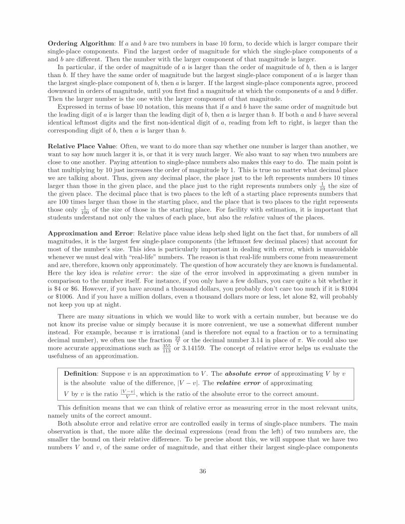
Ordering Algorithm: If a and b are two numbers in base 10 form, to decide which is larger compare theirsingle-place components. Find the largest order of magnitude for which the single-place components of aand b are different. Then the number with the larger component of that magnitude is larger.

In particular, if the order of magnitude of a is larger than the order of magnitude of b, then a is largerthan b. If they have the same order of magnitude but the largest single-place component of a is larger thanthe largest single-place component of b, then a is larger. If the largest single-place components agree, proceeddownward in orders of magnitude, until you first find a magnitude at which the components of a and b differ.Then the larger number is the one with the larger component of that magnitude.

Expressed in terms of base 10 notation, this means that if a and b have the same order of magnitude butthe leading digit of a is larger than the leading digit of b, then a is larger than b. If both a and b have severalidentical leftmost digits and the first non-identical digit of a, reading from left to right, is larger than thecorresponding digit of b, then a is larger than b.

Relative Place Value: Often, we want to do more than say whether one number is larger than another, wewant to say how much larger it is, or that it is very much larger. We also want to say when two numbers areclose to one another. Paying attention to single-place numbers also makes this easy to do. The main point isthat multiplying by 10 just increases the order of magnitude by 1. This is true no matter what decimal placewe are talking about. Thus, given any decimal place, the place just to the left represents numbers 10 timeslarger than those in the given place, and the place just to the right represents numbers only 1

10 the size ofthe given place. The decimal place that is two places to the left of a starting place represents numbers thatare 100 times larger than those in the starting place, and the place that is two places to the right representsthose only 1

100 of the size of those in the starting place. For facility with estimation, it is important thatstudents understand not only the values of each place, but also the relative values of the places.

Approximation and Error: Relative place value ideas help shed light on the fact that, for numbers of allmagnitudes, it is the largest few single-place components (the leftmost few decimal places) that account formost of the number’s size. This idea is particularly important in dealing with error, which is unavoidablewhenever we must deal with “real-life” numbers. The reason is that real-life numbers come from measurementand are, therefore, known only approximately. The question of how accurately they are known is fundamental.Here the key idea is relative error : the size of the error involved in approximating a given number incomparison to the number itself. For instance, if you only have a few dollars, you care quite a bit whether itis $4 or $6. However, if you have around a thousand dollars, you probably don’t care too much if it is $1004or $1006. And if you have a million dollars, even a thousand dollars more or less, let alone $2, will probablynot keep you up at night.

There are many situations in which we would like to work with a certain number, but because we donot know its precise value or simply because it is more convenient, we use a somewhat different numberinstead. For example, because π is irrational (and is therefore not equal to a fraction or to a terminatingdecimal number), we often use the fraction 22

7 or the decimal number 3.14 in place of π. We could also usemore accurate approximations such as 355

113 or 3.14159. The concept of relative error helps us evaluate theusefulness of an approximation.

Definition: Suppose v is an approximation to V . The absolute error of approximating V by v

is the absolute value of the difference, |V − v|. The relative error of approximating

V by v is the ratio |V −v|V , which is the ratio of the absolute error to the correct amount.

This definition means that we can think of relative error as measuring error in the most relevant units,namely units of the correct amount.

Both absolute error and relative error are controlled easily in terms of single-place numbers. The mainobservation is that, the more alike the decimal expressions (read from the left) of two numbers are, thesmaller the bound on their relative difference. To be precise about this, we will suppose that we have twonumbers V and v, of the same order of magnitude, and that either their largest single-place components

36

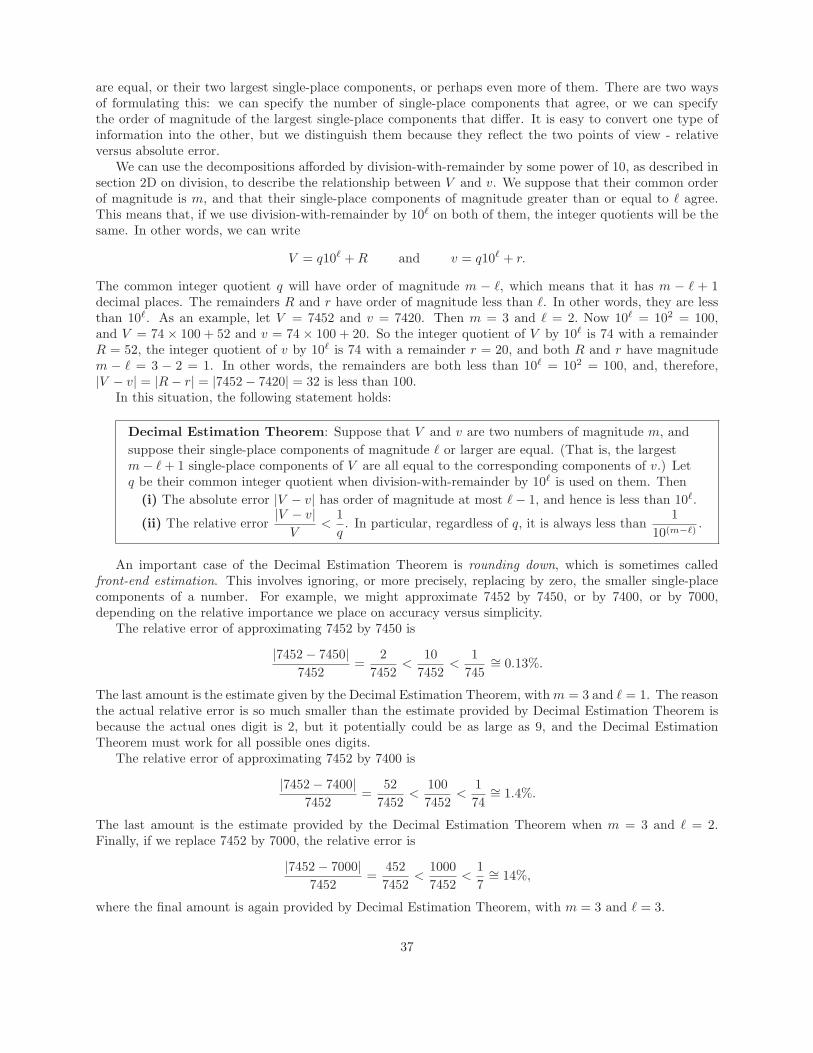
are equal, or their two largest single-place components, or perhaps even more of them. There are two waysof formulating this: we can specify the number of single-place components that agree, or we can specifythe order of magnitude of the largest single-place components that differ. It is easy to convert one type ofinformation into the other, but we distinguish them because they reflect the two points of view - relativeversus absolute error.

We can use the decompositions afforded by division-with-remainder by some power of 10, as described insection 2D on division, to describe the relationship between V and v. We suppose that their common orderof magnitude is m, and that their single-place components of magnitude greater than or equal to � agree.This means that, if we use division-with-remainder by 10� on both of them, the integer quotients will be thesame. In other words, we can write

V = q10� + R and v = q10� + r.

The common integer quotient q will have order of magnitude m − �, which means that it has m − � + 1decimal places. The remainders R and r have order of magnitude less than �. In other words, they are lessthan 10�. As an example, let V = 7452 and v = 7420. Then m = 3 and � = 2. Now 10� = 102 = 100,and V = 74 × 100 + 52 and v = 74 × 100 + 20. So the integer quotient of V by 10� is 74 with a remainderR = 52, the integer quotient of v by 10� is 74 with a remainder r = 20, and both R and r have magnitudem − � = 3 − 2 = 1. In other words, the remainders are both less than 10� = 102 = 100, and, therefore,|V − v| = |R− r| = |7452− 7420| = 32 is less than 100.

In this situation, the following statement holds:

Decimal Estimation Theorem: Suppose that V and v are two numbers of magnitude m, andsuppose their single-place components of magnitude � or larger are equal. (That is, the largestm− � + 1 single-place components of V are all equal to the corresponding components of v.) Letq be their common integer quotient when division-with-remainder by 10� is used on them. Then

(i) The absolute error |V − v| has order of magnitude at most �− 1, and hence is less than 10�.

(ii) The relative error|V − v|

V<

1q. In particular, regardless of q, it is always less than

110(m−�)

.

An important case of the Decimal Estimation Theorem is rounding down, which is sometimes calledfront-end estimation. This involves ignoring, or more precisely, replacing by zero, the smaller single-placecomponents of a number. For example, we might approximate 7452 by 7450, or by 7400, or by 7000,depending on the relative importance we place on accuracy versus simplicity.

The relative error of approximating 7452 by 7450 is

|7452− 7450|7452

=2

7452<

107452

<1

745∼= 0.13%.

The last amount is the estimate given by the Decimal Estimation Theorem, with m = 3 and � = 1. The reasonthe actual relative error is so much smaller than the estimate provided by Decimal Estimation Theorem isbecause the actual ones digit is 2, but it potentially could be as large as 9, and the Decimal EstimationTheorem must work for all possible ones digits.

The relative error of approximating 7452 by 7400 is

|7452− 7400|7452

=52

7452<

1007452

<174∼= 1.4%.

The last amount is the estimate provided by the Decimal Estimation Theorem when m = 3 and � = 2.Finally, if we replace 7452 by 7000, the relative error is

|7452− 7000|7452

=4527452

<10007452

<17∼= 14%,

where the final amount is again provided by Decimal Estimation Theorem, with m = 3 and � = 3.

37

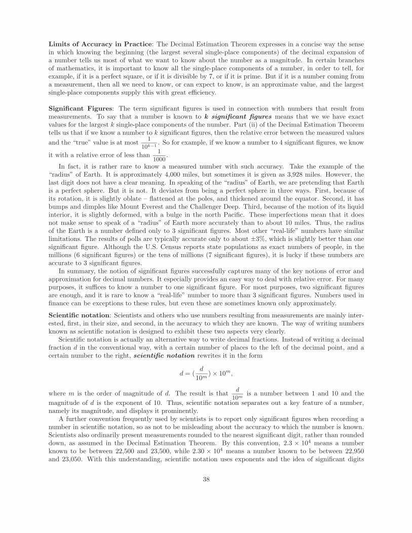
Limits of Accuracy in Practice: The Decimal Estimation Theorem expresses in a concise way the sensein which knowing the beginning (the largest several single-place components) of the decimal expansion ofa number tells us most of what we want to know about the number as a magnitude. In certain branchesof mathematics, it is important to know all the single-place components of a number, in order to tell, forexample, if it is a perfect square, or if it is divisible by 7, or if it is prime. But if it is a number coming froma measurement, then all we need to know, or can expect to know, is an approximate value, and the largestsingle-place components supply this with great efficiency.

Significant Figures: The term significant figures is used in connection with numbers that result frommeasurements. To say that a number is known to k significant figures means that we we have exactvalues for the largest k single-place components of the number. Part (ii) of the Decimal Estimation Theoremtells us that if we know a number to k significant figures, then the relative error between the measured valuesand the “true” value is at most 1

10k−1. So for example, if we know a number to 4 significant figures, we know

it with a relative error of less than 1

1000.

In fact, it is rather rare to know a measured number with such accuracy. Take the example of the“radius” of Earth. It is approximately 4,000 miles, but sometimes it is given as 3,928 miles. However, thelast digit does not have a clear meaning. In speaking of the “radius” of Earth, we are pretending that Earthis a perfect sphere. But it is not. It deviates from being a perfect sphere in three ways. First, because ofits rotation, it is slightly oblate – flattened at the poles, and thickened around the equator. Second, it hasbumps and dimples like Mount Everest and the Challenger Deep. Third, because of the motion of its liquidinterior, it is slightly deformed, with a bulge in the north Pacific. These imperfections mean that it doesnot make sense to speak of a “radius” of Earth more accurately than to about 10 miles. Thus, the radiusof the Earth is a number defined only to 3 significant figures. Most other “real-life” numbers have similarlimitations. The results of polls are typically accurate only to about ±3%, which is slightly better than onesignificant figure. Although the U.S. Census reports state populations as exact numbers of people, in themillions (6 significant figures) or the tens of millions (7 significant figures), it is lucky if these numbers areaccurate to 3 significant figures.

In summary, the notion of significant figures successfully captures many of the key notions of error andapproximation for decimal numbers. It especially provides an easy way to deal with relative error. For manypurposes, it suffices to know a number to one significant figure. For most purposes, two significant figuresare enough, and it is rare to know a “real-life” number to more than 3 significant figures. Numbers used infinance can be exceptions to these rules, but even these are sometimes known only approximately.

Scientific notation: Scientists and others who use numbers resulting from measurements are mainly inter-ested, first, in their size, and second, in the accuracy to which they are known. The way of writing numbersknown as scientific notation is designed to exhibit these two aspects very clearly.

Scientific notation is actually an alternative way to write decimal fractions. Instead of writing a decimalfraction d in the conventional way, with a certain number of places to the left of the decimal point, and acertain number to the right, scientific notation rewrites it in the form

d = (d

10m)× 10m,

where m is the order of magnitude of d. The result is that d

10mis a number between 1 and 10 and the

magnitude of d is the exponent of 10. Thus, scientific notation separates out a key feature of a number,namely its magnitude, and displays it prominently.

A further convention frequently used by scientists is to report only significant figures when recording anumber in scientific notation, so as not to be misleading about the accuracy to which the number is known.Scientists also ordinarily present measurements rounded to the nearest significant digit, rather than roundeddown, as assumed in the Decimal Estimation Theorem. By this convention, 2.3 × 104 means a numberknown to be between 22,500 and 23,500, while 2.30 × 104 means a number known to be between 22,950and 23,050. With this understanding, scientific notation uses exponents and the idea of significant digits

38

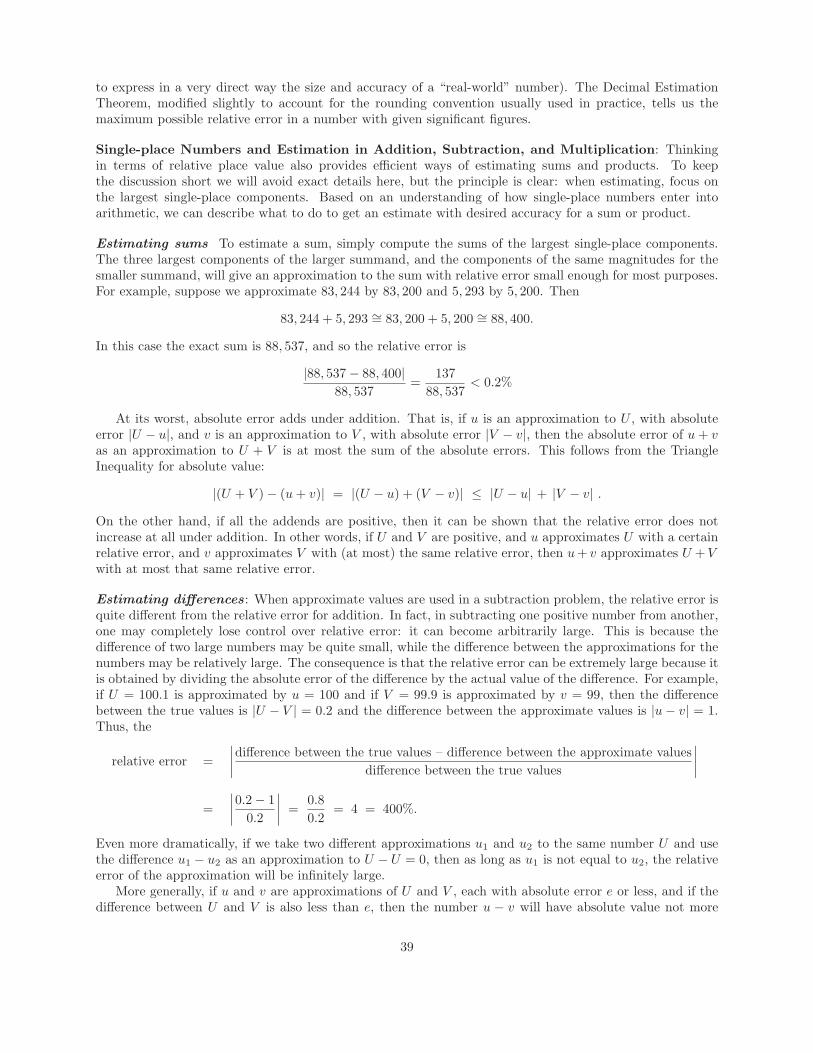
to express in a very direct way the size and accuracy of a “real-world” number). The Decimal EstimationTheorem, modified slightly to account for the rounding convention usually used in practice, tells us themaximum possible relative error in a number with given significant figures.

Single-place Numbers and Estimation in Addition, Subtraction, and Multiplication: Thinkingin terms of relative place value also provides efficient ways of estimating sums and products. To keepthe discussion short we will avoid exact details here, but the principle is clear: when estimating, focus onthe largest single-place components. Based on an understanding of how single-place numbers enter intoarithmetic, we can describe what to do to get an estimate with desired accuracy for a sum or product.

Estimating sums To estimate a sum, simply compute the sums of the largest single-place components.The three largest components of the larger summand, and the components of the same magnitudes for thesmaller summand, will give an approximation to the sum with relative error small enough for most purposes.For example, suppose we approximate 83, 244 by 83, 200 and 5, 293 by 5, 200. Then

83, 244 + 5, 293 ∼= 83, 200 + 5, 200 ∼= 88, 400.

In this case the exact sum is 88, 537, and so the relative error is

|88, 537− 88, 400|88, 537

=137

88, 537< 0.2%

At its worst, absolute error adds under addition. That is, if u is an approximation to U , with absoluteerror |U − u|, and v is an approximation to V , with absolute error |V − v|, then the absolute error of u + vas an approximation to U + V is at most the sum of the absolute errors. This follows from the TriangleInequality for absolute value:

|(U + V )− (u + v)| = |(U − u) + (V − v)| ≤ |U − u| + |V − v| .On the other hand, if all the addends are positive, then it can be shown that the relative error does notincrease at all under addition. In other words, if U and V are positive, and u approximates U with a certainrelative error, and v approximates V with (at most) the same relative error, then u + v approximates U + Vwith at most that same relative error.

Estimating differences: When approximate values are used in a subtraction problem, the relative error isquite different from the relative error for addition. In fact, in subtracting one positive number from another,one may completely lose control over relative error: it can become arbitrarily large. This is because thedifference of two large numbers may be quite small, while the difference between the approximations for thenumbers may be relatively large. The consequence is that the relative error can be extremely large because itis obtained by dividing the absolute error of the difference by the actual value of the difference. For example,if U = 100.1 is approximated by u = 100 and if V = 99.9 is approximated by v = 99, then the differencebetween the true values is |U − V | = 0.2 and the difference between the approximate values is |u− v| = 1.Thus, the

relative error =∣∣∣∣difference between the true values – difference between the approximate values

difference between the true values

∣∣∣∣

=∣∣∣∣0.2− 1

0.2

∣∣∣∣ =

0.80.2

= 4 = 400%.

Even more dramatically, if we take two different approximations u1 and u2 to the same number U and usethe difference u1 − u2 as an approximation to U − U = 0, then as long as u1 is not equal to u2, the relativeerror of the approximation will be infinitely large.

More generally, if u and v are approximations of U and V , each with absolute error e or less, and if thedifference between U and V is also less than e, then the number u − v will have absolute value not more

39

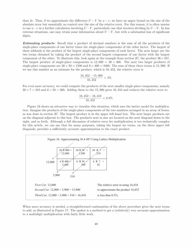
than 2e. Thus, if we approximate the difference U − V by u− v, we have an upper bound on the size of theabsolute error but essentially no control over the size of the relative error. For this reason, it is often unwiseto use u−v in a further calculation involving U−V , particularly one that involves dividing by U−V . In lessextreme situations, one may retain some information about U − V , but with a substantial loss of significantdigits.

Estimating products: Recall that a product of decimal numbers is the sum of all the products of thesingle-place components of one factor times the single-place components of the other factor. The largest ofthese addends is the product of the largest single-place components of each factor. The next larger are thetwo terms obtained by taking the product of the second largest component of one factor with the largestcomponent of the other. To illustrate this, look again at the example from section 2C, the product 36× 457.The largest product of single-place components is 12, 000 = 30 × 400. The next two larger products ofsingle-place components are 30× 50 = 1500 and 6× 400 = 2400. The sum of these three terms is 15, 900. Ifwe use this number as an estimate for the product, which is 16, 452, the relative error is

16, 452− 15, 90016, 452

< 4%.

For even more accuracy, we could compute the products of the next smaller single-place components, namely30× 7 = 210 and 6× 50 = 300. Adding these to the 15, 900 gives 16, 410 and reduces the relative error to

16, 452− 16, 41016, 452

< 0.3%.

Figure 16 shows an attractive way to visualize this situation, which uses the lattice model for multiplica-tion. Imagine the products of the single-place components of the two numbers arranged in an array of boxes,as was done in section 2C. The largest product is in the upper left-hand box. The next larger products areon the diagonal adjacent to this box. The products next in size are located on the next diagonal down to theright, and so forth. Although a full discussion of relative error for multiplication is too technically complexfor this article, we can say that for many purposes, taking the largest six terms, on the three upper leftdiagonals, provides a sufficiently accurate approximation to the exact product.

30 X 400 = 12,000

30 X 50 = 1,500

30 X 7 = 210

6 X 400 = 2,400

6 X 50 = 300

6 X 7 = 42

Figure 16: Approximating 36 x 487 Using Lattice Multiplication

First Cut: 12,000Second Cut: 12,000 + 3,900 = 15,900

Third Cut: 12,000 + 3,900 + 510 = 16,410

12,000

3,900 510

The relative error in using 16,410 to approximate the product 16,452

is less than 0.3%.

When more accuracy is needed, a straightforward continuation of the above procedure gives the next termsto add, as illustrated in Figure 17. The upshot is a method to get a (relatively) very accurate approximationto a multidigit multiplication with fairly little work.

40

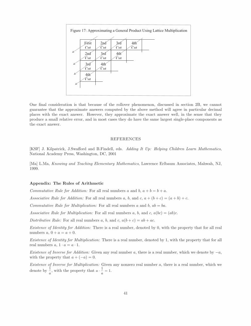
First Cut

2nd Cut

3rd Cut

4th Cut

2nd Cut

3rd Cut

4th Cut

3rd Cut

4th Cut

4th Cut

Figure 17: Approximating a General Product Using Lattice Multiplication

One final consideration is that because of the rollover phenomenon, discussed in section 2B, we cannotguarantee that the approximate answers computed by the above method will agree in particular decimalplaces with the exact answer. However, they approximate the exact answer well, in the sense that theyproduce a small relative error, and in most cases they do have the same largest single-place components asthe exact answer.

REFERENCES

[KSF] J. Kilpatrick, J.Swafford and B.Findell, eds. Adding It Up: Helping Children Learn Mathematics,National Academy Press, Washington, DC, 2001

[Ma] L.Ma, Knowing and Teaching Elementary Mathematics, Lawrence Erlbaum Associates, Mahwah, NJ,1999.

Appendix: The Rules of Arithmetic

Commutative Rule for Addition: For all real numbers a and b, a + b = b + a.

Associative Rule for Addition: For all real numbers a, b, and c, a + (b + c) = (a + b) + c.

Commutative Rule for Multiplication: For all real numbers a and b, ab = ba.

Associative Rule for Multiplication: For all real numbers a, b, and c, a(bc) = (ab)c.

Distributive Rule: For all real numbers a, b, and c, a(b + c) = ab + ac.

Existence of Identity for Addition: There is a real number, denoted by 0, with the property that for all realnumbers a, 0 + a = a + 0.

Existence of Identity for Multiplication: There is a real number, denoted by 1, with the property that for allreal numbers a, 1 · a = a · 1.

Existence of Inverse for Addition: Given any real number a, there is a real number, which we denote by −a,with the property that a + (−a) = 0.

Existence of Inverse for Multiplication: Given any nonzero real number a, there is a real number, which wedenote by 1

a, with the property that a · 1

a= 1.

41