taking stock: monetary policy transmission to equity markets

Taking Stock: Monetary Policy Transmission to Equity Markets

Ehrmann, Michael, 1968-Fratzscher, Marcel.

Journal of Money, Credit, and Banking, Volume 36, Number 4, August2004, pp. 719-737 (Article)

Published by The Ohio State University PressDOI: 10.1353/mcb.2004.0063

For additional information about this article

Access Provided by University of Virginia Libraries __ACCESS_STATEMENT__ (Viva) at 09/27/12 4:05AM GMT

http://muse.jhu.edu/journals/mcb/summary/v036/36.4ehrmann.html

http://muse.jhu.edu/journals/mcb/summary/v036/36.4ehrmann.html

MICHAEL EHRMANN

MARCEL FRATZSCHER

Taking Stock: Monetary Policy Transmission

to Equity Markets

This paper analyses the effects of U.S. monetary policy on stock markets. Wepresent evidence that individual stocks react in a highly heterogeneousfashion to U.S. monetary policy shocks and relate this heterogeneity tofinancial constraints and Tobin’s q. First, we show that there are strongindustry-specific effects of U.S. monetary policy. Second, we also find thatfor the 500 individual stocks comprising the S&P500 the firms with lowcash flows, small size, poor credit ratings, low debt to capital ratios, highprice-earnings ratios, or a high Tobin’s q are affected significantly moreby monetary policy.

JEL codes: G14, E44, E52Keywords: monetary policy, stock market, credit channel, Tobin’s q, finan-

cial constraints, S&P500.

One central argument of James Tobin’s seminal 1969Journal of Money, Credit and Banking paper was that “financial policies” can playa crucial role in altering what later became known as Tobin’s q, the market valueof a firm’s assets relative to their replacement costs. Tobin emphasized that, inparticular, monetary policy can change this ratio. This 1969 JMCB paper togetherwith another of his contributions (Tobin 1978) became a key element in the formula-tion and understanding of the stock market channel of monetary policy transmission.Tobin’s argument in this work was that a tightening of monetary policy, which mayresult from an increase in inflation, lowers the present value of future earning flowsand hence depresses equity markets.

We would like to thank Giovanni Favara, Anil Kashyap, Francisco Maeso-Fernandez, Paul Mizen,Brian Sack, Anna Sanz de Galdeano, Plutarchos Sakellaris, Frank Smets, Philip Vermeulen, and theeditor, Ken West, as well as an anonymous referee and seminar participants at the Tobin Symposiumat the Chicago Fed, and at the ECB for comments and discussions, and Reuters for providing some ofthe data series. This paper presents the authors’ personal opinions and does not necessarily reflect theviews of the European Central Bank.

Michael Ehrmann is Principal Economist at the European Central Bank. E-mail:michael.ehrmannecb.int Marcel Fratzscher is an Advisor at the European Central Bank.E-mail: marcel.fratzscherecb.int

Received July 21, 2003; and accepted in revised form February 23, 2004.

Journal of Money, Credit, and Banking, Vol. 36, No. 4 (August 2004)Copyright 2004 by The Ohio State University

day

Muse

720 : MONEY, CREDIT, AND BANKING

The second part of Tobin’s argument, namely the relationship between monetarypolicy and equity prices, is still not very well understood. On the one hand, ithas proven difficult to properly identify monetary policy, since monetary policymay be endogenous in that central banks might react to developments in stock markets.Considerable progress has recently been made in this respect. Rigobon and Sack(2002, 2003) develop a methodology that exploits the heteroskedasticity present infinancial markets to identify monetary policy shocks, while Kuttner (2001) andBernanke and Kuttner (2003) derive monetary policy shocks through measures ofmarket expectations obtained from federal funds futures contracts. In this paper, wewill employ a methodology similar to Bernanke and Kuttner (2003), by identifyingmonetary policy shocks through market expectations obtained from surveys ofmarket participants.

On the other hand, more research is needed to understand why individual stocksreact so differently to monetary policy shocks and what the driving force is behindthis reaction. The recent paper by Bernanke and Kuttner (2003) shows that verylittle of the market’s reaction can be attributed to the effect of monetary policy onthe real rate of interest. Rather, the response of stock prices is driven by the impacton expected future excess returns and to some extent on expected future dividends.In this paper, we go a step further by analyzing which factors of these expectations areimportant for understanding the large heterogeneity in the reaction of individualstocks to monetary policy.

In the literature on the credit channel of monetary policy transmission, Bernankeand Blinder (1992) and Kashyap, Stein, and Wilcox (1993) show that a tighteningof monetary policy has a particularly strong impact on firms that are highly bank-dependent borrowers as banks reduce their overall supply of credit. Bernanke andGertler (1989) and Kiyotaki and Moore (1997) argue that worsening credit marketconditions affect firms also by weakening their balance sheets as the present valueof collateral falls with rising interest rates, and that this effect can be stronger forsome firms than for others. Both arguments are based on information asymmetries:firms for which less information is publicly available may find it more difficult toaccess bank loans when credit conditions become tighter as banks tend to reducecredit lines first to those customers about whom they have the least information(Gertler and Hubbard, 1988, Gertler and Gilchrist, 1994). For instance, Thorbecke(1997) and Perez-Quiros and Timmermann (2000) show that the response of stockreturns to monetary policy is larger for small firms.

If a credit channel is at work for firms that are quoted on stock markets, onewould expect that their stock prices respond to monetary policy in a heterogeneousfashion, with the prices of firms that are subject to relatively larger informationalasymmetries reacting more strongly. The reason is that their expected future earningsare affected more, since these firms will find it harder to access funds following amonetary tightening, which should lead to a constraint of the supply of their goods.

Another differentiation of the response of stock prices to monetary policy is likelyto be related to the response of the demand for firms’ products. Firms that producegoods for which demand is highly cyclical or interest-sensitive should see their

MICHAEL EHRMANN AND MARCEL FRATZSCHER : 721

expected future earnings affected relatively more following a monetary policy move.These effects are not based on the credit channel; rather, they arise through the interest-rate channel. Therefore, one would expect that the differentiation of responses tomonetary policy is not only dependent on the firm-specific characteristics, but also onthose of the industry to which the firm is affiliated.

This paper analyses both effects, and aims to distinguish their respective contribu-tions to the overall stock market response. In a first step, we present evidence that theindividual firms included in the S&P500 index react in a highly heterogeneousfashion to U.S. monetary policy shocks. Second, we investigate whether we canidentify industry-specific effects of monetary policy. It is found that cyclical sectors,such as technology, communications, and cyclical consumer goods, react two tothree times stronger to monetary policy than less cyclical sectors.

As a third step, we test whether monetary policy has a stronger effect on theequity returns of firms that are financially constrained and/or have good investmentopportunities. We find strong empirical support for this hypothesis using variousproxies for financial constraints, with large differences in the effects of monetary policyacross firms. We show that firms with low cash flows, poor credit ratings, low debtto capital ratios, high price-earnings ratios, or a high Tobin’s q are affected signifi-cantly more by U.S. monetary policy. For instance, monetary policy affects firmswith poor cash flows or low debt almost twice as much as firms with high cashflows or high debt.

The paper proceeds as follows. Section 1 presents the data employed in this studyand discusses some conceptual issues important for the empirical analysis. Section2 tests the role of the interest rate channel, credit channel, and Tobin’s q in theresponse of equity markets to U.S. monetary policy. Section 3 concludes.

1. MONETARY POLICY AND EQUITY MARKETS: CONCEPTUALISSUES AND DATA

An important issue that arises when measuring the effect of monetary policy onequity markets is the correct identification of monetary policy. Many papers in thisliterature (e.g., Lamont, Polk, and Saa-Requejo, 2001, Perez-Quiros and Timmer-mann, 2000) use changes in market interest rates or official rates as their measuresof monetary policy. The problem with these measures, however, is that changes ininterest rates can coincide with changes in business cycle conditions and otherrelevant economic variables. It is therefore not clear whether the effect attributedto monetary policy in those papers reflects other factors. A number of studieshave therefore followed the example of Christiano, Eichenbaum, and Evans (1994)and extract monetary policy shocks as the orthogonalised innovations from VARmodels. Thorbecke (1997) employs this methodology and finds that for the period1953–90 the response of U.S. stock returns to monetary policy shocks, based onfederal fund rates, differs significantly across industries and that small firms’ returnsreact much more strongly than those of large firms. Patelis (1997) also employs a


related methodology and arrives at very similar results, but also shows that theoverall explanatory power of monetary policy for stock returns is rather low. Conover,Jensen, and Johnson (1999) look at 16 industrialized countries and find that equitymarkets in several of these markets react both to the local as well as to the U.S.“monetary environment,” i.e., to changes in monetary policy.

A central shortcoming of this methodology is, however, that it is subject toan endogeneity bias, i.e. monetary policy shocks that are extracted from structuralVAR models or from changes in interest rates using monthly or quarterly frequenciesare unlikely to be purely exogenous. Rigobon and Sack (2002, 2003) have shownconvincingly that monetary policy reacts to stock market developments in a waythat consistently takes the impact of stock market movements on aggregate demandinto account. The essence of Rigobon and Sack’s argument is that causality betweeninterest rates and equity prices runs in both directions. They show that not accountingfor this endogeneity may introduce a significant bias in empirical estimations of thereaction of equity returns to monetary policy.

To identify monetary policy shocks more accurately, several papers have con-ducted event studies based on higher frequency observations, mostly daily data,analyzing how equity markets react to monetary policy. A seminal paper employingsuch an event-study methodology is that of Cook and Hahn (1989), who test whetherchanges to the federal funds rate affected asset prices during the period 1974–79.Thorbecke (1997) uses the same methodology but extends the data also to the earlyGreenspan period 1987–94 and finds that the U.S. equity index indeed reactedsignificantly to changes in the federal funds rate on days when such changes tookplace.

Other event studies looking at the link between monetary policy and equity returnsare those of Bomfim (2001), Durham (2002), Jensen and Johnson (1995), and Lobo(2000). For instance, Lobo (2000) finds for the period 1990–98 that tightenings inthe federal funds and/or discount rate had a stronger effect on equity marketsthan monetary policy easings. Bomfim (2001) shows that volatility of equitymarkets tends to be relatively lower on days before and higher on days aftermonetary policy decisions.

One shortcoming of the existing event-study literature about monetary policy andequity markets is that monetary policy changes are simply measured as changes ofpolicy rates on days of FOMC meetings. Kuttner (2001) has shown that on the dayof announcements, markets react mostly not to the announcements per se, but totheir unexpected component that is not already priced into the market. This argumentis consistent with the efficient market hypothesis that asset prices should reflect allinformation available at any point in time.

The empirical methodology we use in this paper falls into the category of eventstudies. For the period from February 1994 to February 2003—i.e. since the Feddiscloses decisions concerning the Fed funds rate target—we analyze the effect ofthe surprise component of monetary policy decisions on equity returns on the daysof their announcement. This surprise is measured as the difference between theannouncement of the FOMC decision and the market expectation. The expectations


data for monetary policy decisions originate from a Reuters poll among marketparticipants, conducted on Fridays before each FOMC meeting. We use the meanof the survey as our expectations measure although using the median yields similareconometric results.

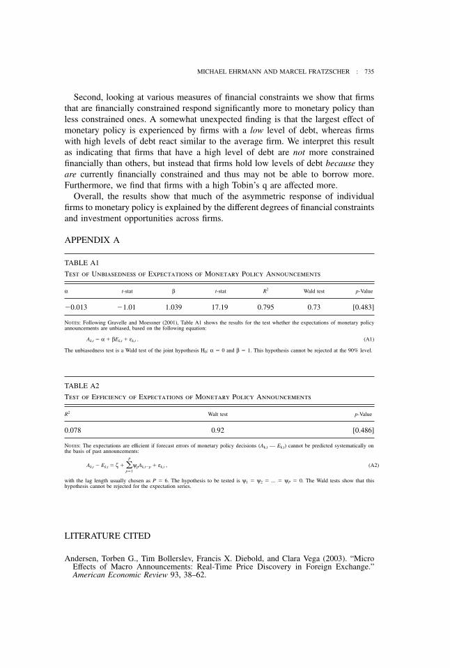
Employing standard techniques in the literature (e.g., Gravelle and Moessner2001), we test for unbiasedness and efficiency of the survey data. Tables A1 andA2 show the results for the respective tests for the forecasts of monetary policyannouncements. We find that the survey expectations are of good quality as they proveto be unbiased and efficient. As shown previously (Ehrmann and Fratzscher 2002,2003) and also tested here in this paper, the survey-based measures perform verysimilar to expectations data based on federal funds futures, as employed by Kuttner(2001) and Bernanke and Kuttner (2003).

For our measure of stock market returns, we use the returns of the S&P500 index,and of the 500 individual stocks therein as in early 2003, with Bloomberg as thesource. This allows us to cover a broad spectrum of industries and firms, and thusto get at the issue of industry—and firm-specific effects of monetary policy. Wecalculate the daily returns as the log-difference of the daily closing quotes.

Obviously, there are various issues in the measurement of both the monetarypolicy surprises and the daily stock returns that merit discussing. Since the Reuterssurveys are conducted on Fridays prior to the FOMC meetings, they cannot captureany change in market expectations that occurs in between. However, we are com-forted by the fact that results are robust to the use of market expectations derivedfrom the Fed funds futures market, where this issue does not arise.

Regarding the measure of stock returns, the choice of a daily frequency aims atstriking a balance between identifiability of exogenous monetary policy surprisesand estimation of sustained stock market effects. At lower frequencies, as wehave argued above, it is difficult to disentangle the response of monetary policy tostock markets and thus to identify monetary policy surprises. Higher frequency data,as used, e.g. by Andersen et al. (2003) for exchange rates, on the other hand, mightcapture overshooting effects that quickly disappear. We therefore assume that effectsfound on a daily basis are likely to reveal the longer-run impact in a more reli-able fashion.

Our sample covers 79 meetings of the FOMC, from February 4, 1994 to January29, 2003. The beginning of the sample coincides with a change in FOMC practices:since 1994, the FOMC announces the Fed fund target rate in openness, whereas before,the market needed to infer the target rate from the Fed’s behavior. We delete the un-scheduled meeting of September 17, 2001, where the FOMC decided to cut interestrates by 50 basis points in response to the events of September 11, for the unusualcircumstances of this interest rate decision. Not all stocks are observed for thefull sample period; on average, we observe stocks for 71 of the FOMC meeting days.

2. INDUSTRY EFFECTS, THE CREDIT CHANNEL AND TOBIN’S q

We now turn to the question of which firms are affected particularly strongly bymonetary policy. Our sample of firms comprises the 500 individual stocks that


currently constitute the S&P500. As a starting point, we test whether and how theS&P500 index responds to surprises. The econometric model used is formulatedas follows:

rt α βst εt , (1)

where rt denotes the stock market return on day t and st the monetary policy surprise.1

We find that a surprise monetary tightening of 100 basis points lowers stock marketreturns by 5.5%, significant at the 1%-level. This is in line with the findings ofBernanke and Kuttner (2003), who find a 5.3% effect, and Rigobon and Sack (2002),who estimate a 6.2% effect, using similar indices and time periods.

As the next step, we use the empirical model of Equation (1) and regress eachfirm’s return series individually on our monetary policy surprises. We find a glaringand large heterogeneity in the response across the 500 stocks in the S&P500 index.Figure 1 shows the distribution of the estimated parameters. They range from 0.44to 0.15, with a mean of 0.06 and a median of 0.05. The distribution is stronglyskewed towards the left. Overall, these results show that the stock market responseto monetary policy is highly asymmetric. Understanding and explaining this asym-metry and heterogeneity is the focus of the remainder of the paper.

As to the empirical methodology, to carry out the analysis in a panel frameworkof 500 stocks, we will turn to panel regressions of the form

ri,t α β1st β2stxi,t τxi,t εi,t , (2)

where xi,t denotes some firm-specific characteristic, which can be either time-varying(e.g., its size or its cash flow to income ratio), or fixed over time (e.g., its industry

Fig 1. Distribution of monetary policy effects across S&P500 stocks

1. As expected, lagged values of the stock market return proved to be insignificant, and were thereforenot included. The estimated parameter for the intercept is generally insignificant. The estimatesare performed for the sample of FOMC meeting days only.


affiliation). If this variable varies with the stock price (e.g., the price-earnings ratio),we enter it with one lag to avoid problems with endogeneity of the regressors.

Contrary to most of the literature on stock market effects, we decided not to runestimates on a stock by stock basis, and then explain the coefficients in a cross-sectional regression, although the time-series dimension of our sample would haveallowed us to do so. Rather, we decided to pool the data for two reasons. First,many of our firm-specific characteristics are time-varying. In a cross-sectional regres-sion, we could not account for changes in these characteristics over time. Second,pooling allows us to take into account a potential cross-sectional correlation ofresiduals, which we consider a realistic assumption for stock market data: a highresidual in one stock is likely to be accompanied by high residuals in other stocks.To account for this dependence across observations, we estimate Equation (2) viaOLS using panel-corrected standard errors (PCSE). This estimator corrects forheteroskedasticity and assumes that residuals are contemporaneously correlatedacross panels, and estimates the covariance of the OLS coefficients as

V (X′X)1X′ΩX(X′X)1 , (3)

where Ω is the covariance matrix of the residuals:

Ω Σm×m ⊗ ITi × Ti,

where I is an identity matrix and Σ the m by m panel-by-panel covariance matrixof the residuals, formulated as

Σ

ij εi′εj

Tij, (4)

where εi and εj are the residuals for panels i and j from Equation (2) and Tij is thenumber of residuals between the panels that can be matched by time period.

This variance estimator corrects for the dependence across observations. Neglect-ing such correlation will lead to decreased estimates of the variance and to a seriousoverestimation of the significance of parameters. As a matter of fact, this effectturns out to be important.

The results are extremely robust to other changes in the model specification, nomatter whether we allow for fixed effects or not, or run the model over all tradingdays and use feasible GLS to allow for the presence of AR(1) autocorrelation withinpanels. We experimented using a lag of stock returns; however, it never turnedout significant, confirming the validity of the efficient market hypothesis in thiscontext. Similarly, using further lags of the monetary policy surprise does not addany explanatory value—the effects are priced into the market within one day.

We checked for robustness with respect to pure time effects by calculating themean of all stock returns on a daily basis, and by subtracting this daily mean fromeach stock, again day-by-day. This does control for pure time effects in the sameway a full set of time dummies would do. All results are robust to this treatment.

Finally, we conducted several other robustness checks. Most importantly, exclud-ing large outliers of monetary policy surprises yields qualitatively similar results


for the estimates. Moreover, we repeated the analysis using monetary policysurprises as calculated by Kuttner (2001) and used in Bernanke and Kuttner (2003),which are derived from federal funds futures markets, i.e. are market-based ratherthan survey-based as the measure used in this paper. All results are qualitatively,and generally quantitatively extremely robust.2

2.1 Industry-Specific Effects

The effect of monetary policy on stock market returns is likely to differ acrossindustries for various reasons. The interest-sensitivity of the demand for products dif-fers. Furthermore, if monetary policy affects exchange rates, tradable goods industriesare likely to be affected more strongly. Finally, changes in the cost of capital inducedby monetary policy are more important for capital-intensive industries. All thesefactors imply that expected future earnings are affected in a heterogeneous fashionacross industries, which should be reflected in the responsiveness of stock returns.We would therefore expect firms in cyclical industries, capital-intensive industries, andindustries that are relatively open to trade to be affected more strongly.

There is only relatively little evidence of the cross-sectional dimension of monetarypolicy effects in the literature to date. Exceptions are Dedola and Lippi (2000) andPeersman and Smets (2002), who analyze the effect of identified VAR shocks onsectoral production indices for five OECD countries and seven countries of the euroarea, respectively. Ganley and Salmon (1997) and Hayo and Uhlenbruck (2000)similarly analyze industry effects in the UK and Germany. In a similar fashion tothe tests employed in this paper, Angeloni and Ehrmann (2003) analyze cross-sectional responses of stock market returns to monetary policy in the euro area.For the U.S., to our knowledge only Bernanke and Kuttner (2003) perform a similaranalysis. Overall, the findings of this literature support the hypotheses expressedabove.

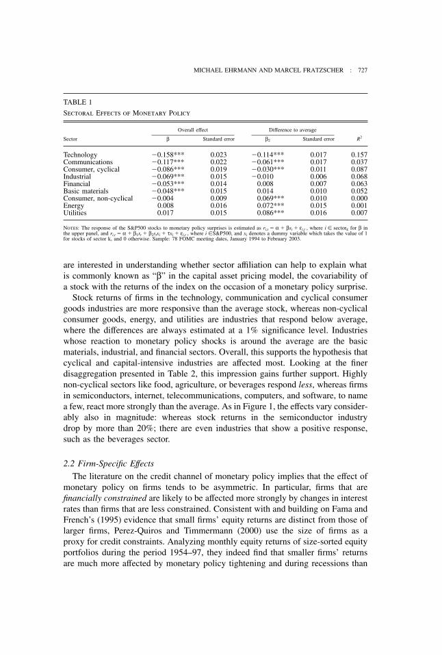
Tables 1 and 2 report results for a breakdown of nine sectors and 60 industrygroups, sorted by the magnitude of monetary policy effects. The left-hand columnsreport results of the panel version of Equation (1), where we repeatedly runregressions with stocks of one sector only. In order to get an assessment of thedifferences across sectors, we also report results from Model (2), where all stocksenter, regardless of their industry affiliation. We run this model repeatedly, eachtime redefining the industry dummy xi to capture stocks with different industryaffiliations.3 The second panels of Tables 1 and 2 report the corresponding resultsfor β2. In that sense, the set of results shown in the second panels controls formarket movements, and aims to estimate how sensitive stock returns of a givenindustry are to monetary policy relative to the market return. In other words, we

2. The tables with these results are available in the Working Paper version, Ehrmann and Fratzscher(2004).

3. Since there is no cross-sectional variation in St, estimating Model (1) including individual stocksshould yield identical results as estimating these models using returns of unweighted industry indices. Weare grateful to the referee for making us aware of this point. Indeed, estimating the models using suchindustry indices produces identical point estimates and standard errors.


TABLE 1

Sectoral Effects of Monetary Policy

Overall effect Difference to average

Sector β Standard error β2 Standard error R2

Technology 0.158*** 0.023 0.114*** 0.017 0.157Communications 0.117*** 0.022 0.061*** 0.017 0.037Consumer, cyclical 0.086*** 0.019 0.030*** 0.011 0.087Industrial 0.069*** 0.015 0.010 0.006 0.068Financial 0.053*** 0.014 0.008 0.007 0.063Basic materials 0.048*** 0.015 0.014 0.010 0.052Consumer, non-cyclical 0.004 0.009 0.069*** 0.010 0.000Energy 0.008 0.016 0.072*** 0.015 0.001Utilities 0.017 0.015 0.086*** 0.016 0.007

Notes: The response of the S&P500 stocks to monetary policy surprises is estimated as ri,t α βst εi,t , where i sectork for β inthe upper panel, and ri,t α β1st β2stxi τxi εi,t , where i S&P500, and xi denotes a dummy variable which takes the value of 1for stocks of sector k, and 0 otherwise. Sample: 78 FOMC meeting dates, January 1994 to February 2003.

are interested in understanding whether sector affiliation can help to explain whatis commonly known as “β” in the capital asset pricing model, the covariability ofa stock with the returns of the index on the occasion of a monetary policy surprise.

Stock returns of firms in the technology, communication and cyclical consumergoods industries are more responsive than the average stock, whereas non-cyclicalconsumer goods, energy, and utilities are industries that respond below average,where the differences are always estimated at a 1% significance level. Industrieswhose reaction to monetary policy shocks is around the average are the basicmaterials, industrial, and financial sectors. Overall, this supports the hypothesis thatcyclical and capital-intensive industries are affected most. Looking at the finerdisaggregation presented in Table 2, this impression gains further support. Highlynon-cyclical sectors like food, agriculture, or beverages respond less, whereas firmsin semiconductors, internet, telecommunications, computers, and software, to namea few, react more strongly than the average. As in Figure 1, the effects vary consider-ably also in magnitude: whereas stock returns in the semiconductor industrydrop by more than 20%; there are even industries that show a positive response,such as the beverages sector.

2.2 Firm-Specific Effects

The literature on the credit channel of monetary policy implies that the effect ofmonetary policy on firms tends to be asymmetric. In particular, firms that arefinancially constrained are likely to be affected more strongly by changes in interestrates than firms that are less constrained. Consistent with and building on Fama andFrench’s (1995) evidence that small firms’ equity returns are distinct from those oflarger firms, Perez-Quiros and Timmermann (2000) use the size of firms as aproxy for credit constraints. Analyzing monthly equity returns of size-sorted equityportfolios during the period 1954–97, they indeed find that smaller firms’ returnsare much more affected by monetary policy tightening and during recessions than

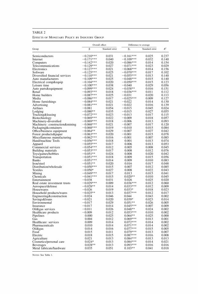
TABLE 2

Effects of Monetary Policy by Industry Group

Overall effect Difference to average

Group β Standard error β2 Standard error R2

Semiconductors 0.210*** 0.031 0.161*** 0.025 0.237Internet 0.171*** 0.040 0.109*** 0.032 0.140Computers 0.142*** 0.020 0.086*** 0.014 0.154Telecommunications 0.129*** 0.027 0.071*** 0.023 0.029Electronics 0.127*** 0.021 0.068*** 0.014 0.156Software 0.125*** 0.025 0.070*** 0.017 0.102Diversified financial services 0.110*** 0.021 0.055*** 0.013 0.140Auto manufacturers 0.109*** 0.025 0.048*** 0.015 0.140Electrical comp&equip 0.104*** 0.020 0.050*** 0.015 0.123Leisure time 0.100*** 0.038 0.040 0.029 0.056Auto parts&equipment 0.099*** 0.024 0.038** 0.016 0.151Retail 0.093*** 0.018 0.036*** 0.011 0.112Home builders 0.087*** 0.025 0.031 0.020 0.113Media 0.086*** 0.017 0.025*** 0.009 0.127Home furnishings 0.084*** 0.021 0.022 0.014 0.130Advertising 0.081*** 0.021 0.022 0.016 0.139Airlines 0.081 0.054 0.015 0.045 0.024Lodging 0.080** 0.035 0.015 0.027 0.055Trucking&leasing 0.072*** 0.023 0.013 0.017 0.115Biotechnology 0.069*** 0.022 0.009 0.018 0.057Machinery-diversified 0.069*** 0.018 0.006 0.013 0.093Machinery: construction&mining 0.068*** 0.021 0.007 0.017 0.120Packaging&containers 0.068*** 0.019 0.010 0.015 0.084Office/business equipment 0.064** 0.029 0.007 0.027 0.042Forest products&paper 0.063*** 0.020 0.001 0.015 0.078Miscellaneous manufacturing 0.062*** 0.016 0.001 0.007 0.085Hand/machine Tools 0.056*** 0.018 0.001 0.013 0.074Apparel 0.055*** 0.017 0.006 0.013 0.053Commercial services 0.054*** 0.012 0.005 0.008 0.045Building materials 0.053*** 0.017 0.008 0.012 0.076Toys/games/hobbies 0.051** 0.024 0.008 0.020 0.042Transportation 0.051*** 0.018 0.009 0.015 0.056Banks 0.051*** 0.014 0.009 0.010 0.083Iron/steel 0.051** 0.020 0.016 0.017 0.048Distribution/wholesale 0.050*** 0.015 0.007 0.012 0.085Textiles 0.050* 0.027 0.008 0.022 0.043Mining 0.049*** 0.017 0.013 0.015 0.041Chemicals 0.041*** 0.015 0.020** 0.010 0.045Entertainment 0.038 0.031 0.026 0.025 0.020Real estate investment trusts 0.029*** 0.009 0.036*** 0.012 0.060Aerospace/defense 0.028** 0.014 0.033*** 0.012 0.009Housewares 0.026 0.019 0.033* 0.018 0.023Household products/wares 0.025** 0.013 0.037*** 0.012 0.017Engineering&construction 0.024 0.046 0.044 0.043 0.002Savings&loans 0.021 0.020 0.039* 0.023 0.014Environmental 0.017 0.029 0.051** 0.026 0.005Insurance 0.017 0.014 0.045*** 0.007 0.009Oil&gas services 0.011 0.026 0.048** 0.024 0.002Healthcare products 0.009 0.012 0.053*** 0.010 0.002Pipelines 0.000 0.025 0.064** 0.025 0.000Gas 0.004 0.012 0.069*** 0.013 0.001Healthcare: services 0.009 0.014 0.072*** 0.014 0.002Pharmaceuticals 0.010 0.014 0.071*** 0.014 0.002Oil&gas 0.014 0.016 0.077*** 0.015 0.005Food 0.015 0.011 0.079*** 0.013 0.007Electric 0.018 0.015 0.087*** 0.016 0.008Agriculture 0.021 0.013 0.084*** 0.013 0.013Cosmetics/personal care 0.024* 0.013 0.084*** 0.014 0.021Beverages 0.028** 0.013 0.093*** 0.016 0.016Metal fabricate/hardware 0.035 0.051 0.103** 0.041 0.018

Notes: See Table 1.


those of larger firms. Using the size of firms as a proxy for the degree of creditconstraints has been widespread. For instance, Gertler and Hubbard (1988) andGertler and Gilchrist (1994) show that small firms are more dependent on bankloans. Nevertheless, a number of papers point out that size is only an imperfect proxyfor the degree of credit constraints and attempt to find other, more direct measures.Lamont, Polk, and Saa-Requejo (2001), building on work by Kaplan and Zin-gales (1997), use a qualitative measure for financial constraints from informationin firms’ annual reports in fulfillment of SEC requirements and regulations.4 Lamont,Polk, and Saa-Requejo (2001) find for the period 1968–97 that financially constrainedfirms exhibit a significant degree of co-movements in terms of stock returns, and thatthis common factor cannot be attributed to the size of firms or other characteristicssuch as industry-specific effects. The important finding of their paper for our purposeis that they do not detect evidence that financially constrained firms react more stronglyto changes in monetary policy or to business cycle conditions than less con-strained ones.

To analyze the role of the credit channel, we borrow from the literature ideas ofseveral proxies for the degree of financial constraints of firms. Following Kaplanand Zingales (1997), we define the term “financial constraint” to imply a wedgebetween internal and external financing of a firm’s investment. Firms with strongerfinancial constraints are those that find it relatively more difficult to raise fundsto finance investment. First, we look at the size of firms, using the number ofemployees as well as the market value of firms as our size variables.

Second, we follow the example of Lamont, Polk, and Saa-Requejo (2001) andKaplan and Zingales (1997) and use several more direct measures of financialconstraints: the cash flow to income ratio and the ratio of debt to total capital. Theunderlying rationale for including these two measures is that a firm can finance invest-ment either by raising funds internally—by using existing cash flows generated—or externally—via bank loans or capital markets. In theory, our priors are that firmswith large cash flows should be more immune to changes in interest rates as theycan rely more on internal financing of investment. One may expect that firms witha lower ratio of debt to capital are affected more by monetary policy becausethey are more bank-dependent and bank-dependent borrowers are hit more stronglyby a change in the supply of credit (Bernanke and Blinder, 1992, Kashyap, Stein,and Wilcox, 1993).

Moreover, we include the price-earnings ratio in our analysis. Finally, we employMoody’s investment rating and Moody’s bank loan rating as two measures offinancial constraints. We would expect that firms with a better rating should find it

4. More precisely, Kaplan and Zingales (1997) test whether various capital and book ratios—thecash flow to capital ratio, Tobin’s q (proxied by firms’ market to book ratios), and the three ratios ofdebt, of dividends, and of cash holdings to total capital—are systematically related to their qualitativemeasure of financial constraints. They do find a significant relationship for most of these variables,though the finding for q is ambiguous, as discussed above in the Introduction. The main focus of thepaper by Kaplan and Zingales (1997) is on the link between investment and financial constraints, anddoes not analyze equity markets.


easier to obtain financing of their investments and therefore should be less affectedby changes in monetary policy.

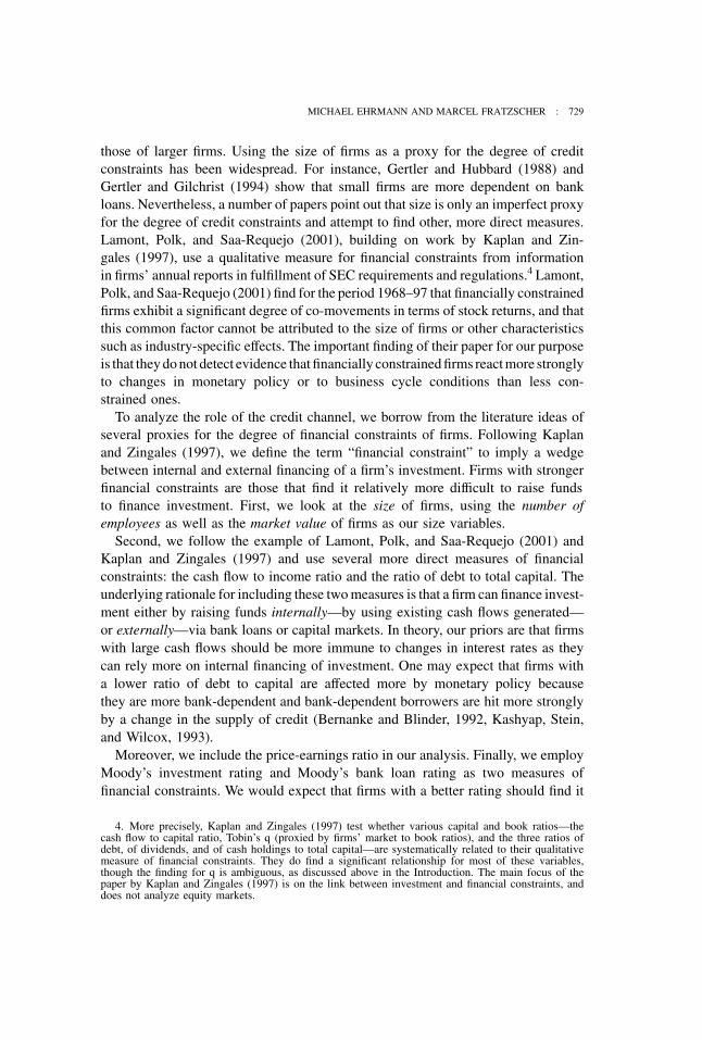
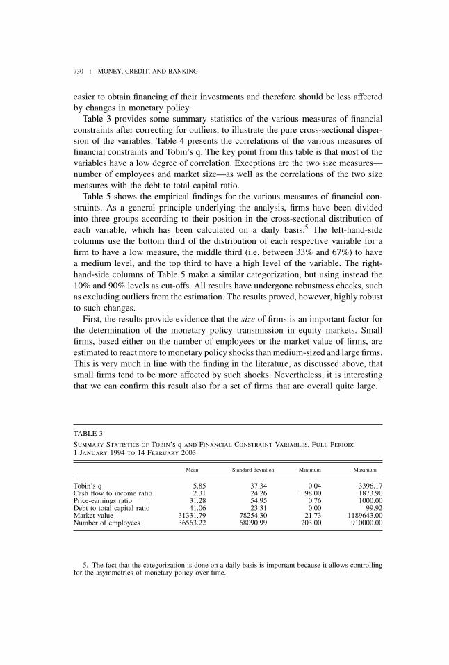
Table 3 provides some summary statistics of the various measures of financialconstraints after correcting for outliers, to illustrate the pure cross-sectional disper-sion of the variables. Table 4 presents the correlations of the various measures offinancial constraints and Tobin’s q. The key point from this table is that most of thevariables have a low degree of correlation. Exceptions are the two size measures—number of employees and market size—as well as the correlations of the two sizemeasures with the debt to total capital ratio.

Table 5 shows the empirical findings for the various measures of financial con-straints. As a general principle underlying the analysis, firms have been dividedinto three groups according to their position in the cross-sectional distribution ofeach variable, which has been calculated on a daily basis.5 The left-hand-sidecolumns use the bottom third of the distribution of each respective variable for afirm to have a low measure, the middle third (i.e. between 33% and 67%) to havea medium level, and the top third to have a high level of the variable. The right-hand-side columns of Table 5 make a similar categorization, but using instead the10% and 90% levels as cut-offs. All results have undergone robustness checks, suchas excluding outliers from the estimation. The results proved, however, highly robustto such changes.

First, the results provide evidence that the size of firms is an important factor forthe determination of the monetary policy transmission in equity markets. Smallfirms, based either on the number of employees or the market value of firms, areestimated to react more to monetary policy shocks than medium-sized and large firms.This is very much in line with the finding in the literature, as discussed above, thatsmall firms tend to be more affected by such shocks. Nevertheless, it is interestingthat we can confirm this result also for a set of firms that are overall quite large.

TABLE 3

Summary Statistics of Tobin’s q and Financial Constraint Variables. Full Period:1 January 1994 to 14 February 2003

Mean Standard deviation Minimum Maximum

Tobin’s q 5.85 37.34 0.04 3396.17Cash flow to income ratio 2.31 24.26 98.00 1873.90Price-earnings ratio 31.28 54.95 0.76 1000.00Debt to total capital ratio 41.06 23.31 0.00 99.92Market value 31331.79 78254.30 21.73 1189643.00Number of employees 36563.22 68090.99 203.00 910000.00

5. The fact that the categorization is done on a daily basis is important because it allows controllingfor the asymmetries of monetary policy over time.


TABLE 4

Cross-correlations of Tobin’s q and Financial Constraint Variables

Cash flow to Debt to total Number ofTobin’s q income ratio Price-earnings ratio capital ratio Market value employees

Tobin’s q 1Cash flow to income ratio 0.0016 1Price-earnings ratio 0.0237 0.0027 1Debt to total capital ratio 0.0362 0.0052 0.1416 1Market value 0.0158 0.0042 0.0482 0.3716 1Number of employees 0.0035 0.0058 0.1049 0.1834 0.5212 1

Second, the results show that firms with low cash flows are affected significantlystronger by U.S. monetary policy shocks. For the 10%–90% categorization, stockreturns of firms with low cash flows respond almost twice as much to monetarypolicy (i.e. 8.8% in response to a 100-bp shock) as compared to firms with highcash flows (i.e. 4.7% to the same shock).

Third, firms that have a good Moody’s investment rating and firms that have agood Moody’s bank loan rating6 are more immune to monetary policy shocks thanthose with a poor rating. Firms with a poor investment rating or with a low bankloan rating react nearly twice as much to monetary policy (6.5% or 6.1%,respectively) than firms with high ratings (3.8% or 3.9%, respectively).

Fourth, the effects for the debt to capital ratio are found to be non-linear: firmswith either high or low values of these ratios respond more to monetary policy thanfirms that have intermediate levels. Overall, the largest effect of monetary policy isrecorded for firms with a low level of debt, whereas firms with high levels ofdebt react similar to the average firm.7 This finding is interesting because it maycome somewhat unexpected. Indeed, this finding conveys a very interesting message.We interpret it as indicating that firms that have a high level of debt are not moreconstrained financially than others. On the contrary, the results suggest that firmshold low levels of debt because they are currently financially constrained andthus may find it relatively more difficult to borrow more. A similar result has beenfound, e.g., in Peersman and Smets (2002) and Dedola and Lippi (2000).

Fifth, firms with a high price earnings ratio are affected more strongly bymonetary policy, indicating that the re-assessment of their earnings expectationsis particularly sensitive to changes in interest rates.

Finally, economic theory is ambiguous about the relationship between monetarypolicy, equity markets and Tobin’s q, as a proxy of investment opportunities andan important corollary of the analyzed financial constraint proxies. On the one

6. Of course, both measures are highly correlated as firms with good investment ratings also tendto have good bank loan ratings.

7. This effect is found to be statistically significant also when comparing the effects of low levelsversus high levels of debt, the test for which is not shown in Table 5.

TAB

LE

5

Tob

in’s

q,Fi

nan

cial

Con

stra

ints

,an

dth

eE

ffec

tsof

Mon

etar

yPo

licy

33%

67

%C

ateg

oriz

atio

na10

%

90%

Cat

egor

izat

iona

β 1

βz,

2St

anda

rder

ror

Diff

eren

ceb

p-V

alue

β 1

βz,

2St

anda

rder

ror

Diff

eren

ceb

p-V

alue

Tobi

n’s

qL

ow

0.04

4***

0.00

80.

050*

0.

055*

**0.

009

0.90

2M

ediu

m

0.05

2***

0.00

9—

0.

056*

**0.

009

—H

igh

0.

076*

**0.

012

0.00

0***

0.

078*

**0.

015

0.02

8**

Cas

hflo

wto

net

inco

me

ratio

Low

0.

078*

**0.

014

0.00

0***

0.

088*

**0.

016

0.00

0***

Med

ium

0.

056*

**0.

012

—

0.06

0***

0.01

3—

Hig

h

0.05

0***

0.01

30.

300

0.

047*

**0.

015

0.19

4Pr

ice-

earn

ings

ratio

Low

0.

053*

**0.

012

0.94

1

0.06

6***

0.01

50.

063*

Med

ium

0.

053*

**0.

012

—

0.05

4***

0.01

2—

Hig

h

0.07

4***

0.01

50.

003*

**

0.09

2***

0.01

90.

002*

**Si

ze:

mar

ket

valu

eL

ow

0.07

2***

0.01

50.

003*

**

0.06

4***

0.01

60.

546

Med

ium

0.

055*

**0.

012

—

0.05

9***

0.01

2—

Hig

h

0.05

5***

0.01

20.

917

0.

065*

**0.

015

0.42

4Si

ze:

num

ber

ofem

ploy

ees

Low

0.

071*

**0.

014

0.01

1**

0.

097*

**0.

018

0.00

0***

Med

ium

0.

054*

**0.

012

—

0.05

6***

0.01

2—

Hig

h

0.05

7***

0.01

30.

601

0.

059*

**0.

015

0.71

2

(Con

tinu

ed)

TAB

LE

5

Con

tin

ued

33%

67

%C

ateg

oriz

atio

na10

%

90%

Cat

egor

izat

iona

β 1

βz,

2St

anda

rder

ror

Diff

eren

ceb

p-V

alue

β 1

βz,

2St

anda

rder

ror

Diff

eren

ceb

p-V

alue

Deb

tto

tota

lca

pita

lra

tioL

ow

0.08

0***

0.01

50.

000*

**

0.13

1***

0.02

00.

000*

**M

ediu

m

0.04

9***

0.01

2—

0.

047*

**0.

012

—H

igh

0.

054*

**0.

012

0.26

7

0.08

4***

0.01

60.

000*

**M

oody

’sin

vest

men

tra

ting

Low

0.

065*

**0.

013

0.00

0***

Hig

h

0.03

8***

0.01

0—

Moo

dy’s

bank

loan

ratin

gL

ow

0.06

1***

0.01

30.

000*

**H

igh

0.

039*

**0.

013

—

Not

es:

a The

cate

gori

zatio

nis

mad

eac

cord

ing

toth

efo

llow

ing

spec

ifica

tion:

each

firm

’sre

spec

tive

vari

able

isde

fined

tobe

“low

”if

itis

inth

ebo

ttom

33%

orin

the

botto

m10

%of

the

vari

able

’sdi

stri

butio

n,“h

igh”

ifit

isin

the

top

33%

or10

%,

and

“med

ium

”ot

herw

ise.

Cat

egor

izat

ion

for

both

Moo

dyra

tings

is“h

igh”

ifth

era

ting

isin

the

Ara

nge,

and

“low

”ot

herw

ise.

b Show

sp-

valu

eof

test

ofth

enu

llhy

poth

eses

that

the

coef

ficie

ntof

low

leve

lan

dhi

ghle

vel

offin

anci

alco

nstr

aint

s,re

spec

tivel

y,is

diff

eren

tfr

omth

em

ediu

mle

vel.

The

test

for

Moo

dy’s

ratin

gsis

for

equa

lity

ofco

effic

ient

sof

low

ratin

gve

rsus

high

ratin

g.T

hees

timat

edm

odel

isan

exte

nsio

nof

Equ

atio

n(2

):

r i,t

α

β 1

s t

z1,

2β z,2

s tx z

,i,t

z1,

2τ zx z

,i,t

ε i,t,

whe

rex 1

(x2)

deno

tes

adu

mm

yva

riab

leth

atde

fines

whe

ther

afir

mbe

long

sto

the

low

(hig

h)ca

tego

riza

tion.


hand, a high q indicates that ample investment opportunities are present for a firm,which may imply, ceteris paribus, that this firm has higher financial constraints byrequiring more external funds to finance this investment. The higher degree ofconstraints may therefore also imply a higher sensitivity of this firm to monetarypolicy shocks. On the other hand, a firm with a relatively high value of its assets(a larger q) may find it easier and may receive more favorable conditions to raiseexternal funds to finance investment. This in turn would imply that firms with alarge q have lower financial constraints and hence they may be less sensitive tomonetary policy shocks.

Following Kaplan and Zingales (1997) and Lamont, Polk and Saa-Requejo (2001),we use firms’ market to book ratios as proxies for Tobin’s q. It is clearly difficultif not impossible to measure q accurately,8 but using the market to book ratio isfairly common in the literature and should provide a reasonably close approximation.

Table 5 reveals that the strongest response of equity returns to monetary policyshocks is experienced by firms with a high q. This difference is sizeable, butsignificant only for the 33%67% categorization.

Overall, the results show that much of the asymmetric response of firms tomonetary policy shocks, as shown in Figure 1, is explained by differences acrossfirms in their degree to which they are financially constrained and to which theyhave different investment opportunities, as proxied by Tobin’s q.9

3. CONCLUSIONS

This paper has analyzed the reaction of equity markets to U.S. monetary policyin the period 1994 to 2003. In particular, this paper has focused on the relativecontributions of the credit channel and the interest rate channel of monetary policytransmission. The empirical methodology employs monetary policy surprises definedas the unexpected component of FOMC announcements on the days of policydecisions. Similar to Bernanke and Kuttner (2003), this empirical measure avoidsthe pitfalls of endogeneity and lack of identification, as outlined by Rigobon andSack (2002, 2003), by instead developing and employing a truly exogenous measureof monetary policy shocks.

As to the results of this paper, we have found evidence that monetary policyaffects individual stocks in a strongly heterogeneous fashion. First, industrial sectorsthat are cyclical and capital-intensive react frequently two to three times strongerto U.S. monetary policy than non-cyclical industries.

8. See Erickson and Whited (2000) for a detailed analysis of the potential importance of measurementerrors in Tobin’s q. The focus of the paper by Erickson and Whited is, however, primarily on therelationship between Tobin’s q and investment.

9. When accounting for the correlations between industry-affiliation and financial constraints andTobin’s q by using a sample based on propensity score matching, it turns out that the significantheterogeneity of the effects of monetary policy on individual stocks prevails. Financial constraints,Tobin’s q, and industry affiliation all play a role, but it is in particular the industry affiliation that is ofcentral importance in explaining the large heterogeneity of firms’ reaction to US monetary policy shocks.See Ehrmann and Fratzscher (2004) for a detailed exposition of this test.


Second, looking at various measures of financial constraints we show that firmsthat are financially constrained respond significantly more to monetary policy thanless constrained ones. A somewhat unexpected finding is that the largest effect ofmonetary policy is experienced by firms with a low level of debt, whereas firmswith high levels of debt react similar to the average firm. We interpret this resultas indicating that firms that have a high level of debt are not more constrainedfinancially than others, but instead that firms hold low levels of debt because theyare currently financially constrained and thus may not be able to borrow more.Furthermore, we find that firms with a high Tobin’s q are affected more.

Overall, the results show that much of the asymmetric response of individualfirms to monetary policy is explained by the different degrees of financial constraintsand investment opportunities across firms.

APPENDIX A

TABLE A1

Test of Unbiasedness of Expectations of Monetary Policy Announcements

α t-stat β t-stat R2 Wald test p-Value

0.013 1.01 1.039 17.19 0.795 0.73 [0.483]

Notes: Following Gravelle and Moessner (2001), Table A1 shows the results for the test whether the expectations of monetary policyannouncements are unbiased, based on the following equation:

Ak,t α βEk,t εk,t . (A1)

The unbiasedness test is a Wald test of the joint hypothesis H0: α 0 and β 1. This hypothesis cannot be rejected at the 90% level.

TABLE A2

Test of Efficiency of Expectations of Monetary Policy Announcements

R2 Walt test p-Value

0.078 0.92 [0.486]

Notes: The expectations are efficient if forecast errors of monetary policy decisions (Ak,t — Ek,t) cannot be predicted systematically onthe basis of past announcements:

Ak,t Ek,t ζ P

p1ψpAk,tp εk,t , (A2)

with the lag length usually chosen as P 6. The hypothesis to be tested is ψ1 ψ2 ... ψP 0. The Wald tests show that thishypothesis cannot be rejected for the expectation series.

LITERATURE CITED

Andersen, Torben G., Tim Bollerslev, Francis X. Diebold, and Clara Vega (2003). “MicroEffects of Macro Announcements: Real-Time Price Discovery in Foreign Exchange.”American Economic Review 93, 38–62.


Angeloni, Ignazio, and Michael Ehrmann (2003). “Monetary Policy Transmission in the EuroArea: Any Changes After EMU?” ECB Working Paper No. 240.

Bernanke, Ben S., and Alan S. Blinder (1992). “The Federal Funds Rate and the Channelsof Monetary Transmission.” American Economic Review 82, 901–921.

Bernanke, Ben, and Mark Gertler (1989). “Agency Costs, Net Worth, and Business Fluctua-tions.” American Economic Review 79, 14–31.

Bernanke, Ben S., and Mark Gertler (1995). “Inside the Black Box: The Credit Channel ofMonetary Policy Transmission.” Journal of Economic Perspectives 9, 27–48.

Bernanke, Ben S., and Kenneth N. Kuttner (2003). “What Explains the Stock Market’sReaction to Federal Reserve Policy?” Mimeo, Board of Governors and Federal ReserveBank of New York.

Bomfim, Antulio N. (2001). “Pre-Announcement Effects, News Effects, and Volatility: Mone-tary Policy and the Stock Market.” Journal of Banking and Finance 27, 133–151.

Brainard, William C., and James Tobin (1968). “Pitfalls in Financial Model Building.”American Economic Review Papers and Proceedings 58, 99–122.

Buiter, Willem H. (2003). “James Tobin: An Appreciation of His Contributions to Economics.”NBER Working Paper No. 9753.

Christiano, Lawrence J., Martin Eichenbaum, and Charles Evans (1996). “The Effects ofMonetary Policy Shocks: Evidence from the Flow of Funds.” Review of Economics andStatistics 78, 16–34.

Conover, C. Mitchell, Gerald R. Jensen, and Robert R. Johnson (1999). “Monetary Environ-ments and International Stock Returns.” Journal of Banking and Finance 23, 1357–1381.

Cook, Timothy, and Thomas Hahn (1989). “The Effect of Changes in the Federal Funds RateTarget on Market Interest Rates in the 1970s.” Journal of Monetary Economics 24, 331–351.

Dedola, Luca, and Francesco Lippi (2000). “The Monetary Transmission Mechanism: Evi-dence from the Industries of Five OECD Countries.” CEPR Discussion Paper No. 2508.

Ehrmann, Michael, and Marcel Fratzscher (2002). “Interdependence between the Euro Areaand the United States: What Role for EMU?” ECB Working Paper Series No. 200.

Ehrmann, Michael, and Marcel Fratzscher (2003). “Monetary Policy Announcements andMoney Markets: A Transatlantic Perspective.” International Finance 6, 309–328.

Ehrmann, Michael, and Marcel Fratzscher (2004). “Taking Stock: Monetary Policy Transmis-sion to Equity Markets. ECB Working Paper Series No. 354.

Erickson, Timothy, and Toni M. Whited (2000). “Measurement Error and the Relationshipbetween Investment and q.” Journal of Political Economy 108, 1027–1057.

Fama, Eugene F., and Kenneth R. French (1995). “Size and Book-to-Market Factors inEarnings and Returns.” Journal of Finance 50, 131–155.

Fuhrer, Jeffrey C., and George R. Moore (1995). “Monetary Policy Trade-offs and the Correla-tion between Nominal Interest Rates and Real Output.” American Economic Review 85,219–239.

Ganley, Joe, and Chris Salmon (1997). “The Industrial Impact of Monetary Policy Shocks:Some Stylised Facts.” Bank of England Working Paper Series No. 68.

Gertler, Mark, and Simon Gilchrist (1994). “Monetary Policy, Business Cycles, and theBehavior of Small Manufacturing Firms.” Quarterly Journal of Economics 109, 309–340.

Gertler, Mark, and R. Glenn Hubbard (1988). “Financial Factors in Business Fluctuations.”NBER Working Paper No. 2758.

Hayo, Bernd, and Birgit Uhlenbrock (2000). “Industry Effects of Monetary Policy in Ger-many.” In Regional Aspects of Monetary Policy in Europe, edited by J. von Hagen, andC. Waller, pp. 127–158. Boston: Kluwer.


Jensen, Gerald R., and Johnson, R.R. (1995). “Discount Rate Changes and Security Returnsin the US, 1962–1991.” Journal of Banking and Finance 19, 79–95.

Jensen, Gerald R., Jeffrey M. Mercer, and Robert R. Johnson (1996). “Business Conditions,Monetary Policy and Expected Security Returns.” Journal of Financial Economics 40,213–237.

Kaplan, Steven N., and Luigi Zingales (1997). “Do Investment Cash Flow SensitivitiesProvide Useful Measures of Financing Constraints.” Quarterly Journal of Economics 112,169–215.

Kashyap, Anil K., Jeremy C. Stein, and David W. Wilcox (1993). “Monetary Policy andCredit Conditions: Evidence from the Composition of External Finance.” American Eco-nomic Review 83, 78–98.

Kiyotaki, Nobuhiro, and John Moore (1997). “Credit Cycles.” Journal of Political Economy105, 211–248.

Kuttner, Kenneth N. (2001). “Monetary Policy Surprises and Interest Rates: Evidence fromthe Fed Funds Futures Market.” Journal of Monetary Economics 47, 523–544.

Lamont, Owen, Christopher Polk, and Jesus Saa-Requejo (2001). “Financial Constraints andStock Returns.” Review of Financial Studies 14, 529–554.

Lobo, Bento J. (2000). “Asymmetric Effects of Interest Rate Changes on Stock Prices.” TheFinancial Review 35, 125–144.

Patelis, Alex D. (1997). “Stock Return Predictability: The Role of Monetary Policy.” Journalof Finance 52, 1951–1972.

Peersman, Geert, and Frank Smets (2002). “The Industry Effects of Monetary Policy in theEuro Area.” ECB Working Paper No. 165.

Perez-Quiros, Gabriel, and Allan Timmermann (2000). “Firm Size and Cyclical Variationsin Stock Returns.” Journal of Finance 55, 1229–1262.

Rigobon, Roberto, and Brian Sack (2002). “The Impact of Monetary Policy on Asset Prices.”NBER Working Paper No. 8794.

Rigobon, Roberto, and Brian Sack (2003). “Measuring the Response of Monetary Policy tothe Stock Market.” Quarterly Journal of Economics 118, 639–669.

Thorbecke, Willem (1997). “On Stock Market Returns and Monetary Policy.” Journal ofFinance 52, 635–654.

Thornton, Daniel (1998). “Tests of the Market’s Reaction to Federal Funds Rate TargetChanges.” Review Federal Reserve Bank of St. Louis, 25–36.

Tobin, James (1969). “A General Equilibrium Approach to Monetary Theory.” Journal ofMoney, Credit and Banking 1, 15–29.

Tobin, James (1978). “Monetary Policy and the Economy: the Transmission Mechanism.”Southern Economic Journal 44, 421–431.

taking stock: monetary policy transmission to equity markets

Documents