Target tracking using WSN

Vinod Kulathumani

West Virginia University

2

Influence field (IF)

• IF of object j wrt given sensing modality: region wherein j can be detected by a sensor of this type

Experimentally measured soldier and vehicle influence fields wrt magnetometer

o Characterized by size and shape which depends on physical characteristics of object

o With sufficient density, estimating IF reduces to measuring number and distribution of sensors detecting j

3

Influence field (2)

• Differences in sizes and/or shapes of estimated influence fields form basis for classification and tracking of objects

• Influence Field Estimation

node-friendly

each node inside influence field only has to detect presence of object

network-friendly

each detecting node transmits only one time-stamped presence bit to the aggregator

robust

inherently spatially distributed, hence tolerant to individual sensor failures

4

Tracking using influence field

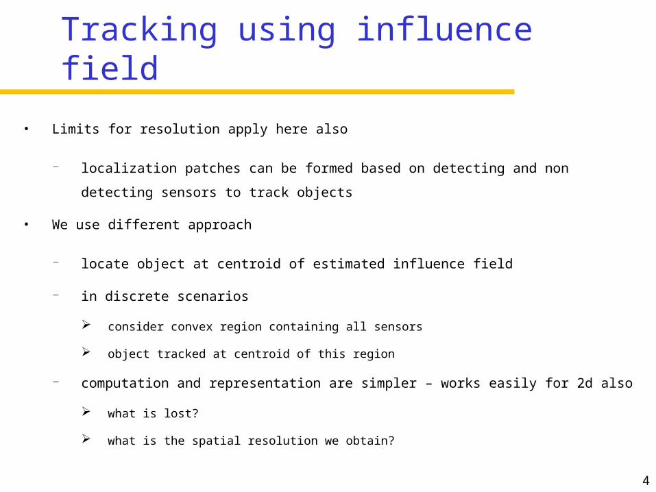
• Limits for resolution apply here also

localization patches can be formed based on detecting and non detecting

sensors to track objects

• We use different approach

locate object at centroid of estimated influence field

in discrete scenarios

consider convex region containing all sensors

object tracked at centroid of this region

computation and representation are simpler – works easily for 2d also

what is lost?

what is the spatial resolution we obtain?

5

Tracking using influence field

• Model

only 1 type of object

all sensors within distance R and none beyond distance R of object

detect objectObject

R

6

Tracking using influence field

• Tracking by centroid

low computational and representative complexity

does not consider negative information

Object

Object estimated

7

Differential Games on Large Scale Sensor Networks

8

Differential Games

• Dynamic Interaction of Agents with Conflicting Interests [Isaacs 75]

Pursuit Evasion Games

Asset Protection

Economy

• Classical Theory assumes global state of the game is observable by the players at all times.

Target

9

Tracking and Pursuit with Sensor Networks

• We study Differential Games when players track the game state through a WSN

•Formulate Solution and Equilibrium Concepts for Networked Games

•Derive Network Requirements for Optimal Pursuit

10

Tracking and Pursuit with Sensor Networks

• Main Results:

Network Requirements for Optimal Pursuit depends on the game state.

Optimal Pursuit in the Asset Protection Game requires the sampling

period and the network delays to scale linearly with the pursuer and evader distance

The pursuer should be able to dictate the information refresh rate based on the state of the game. Network Delay Performance should improve with decreasing distance between source and sink

11

Optimal Pursuit under Communication ConstraintsDiscrete Time Updates

•Optimal pursuit-evasion strategies of the perfect information game is the Nash equilibrium of the game with discrete time updates if

12

Optimal Pursuit under Communication ConstraintsDiscrete Time Updates

13

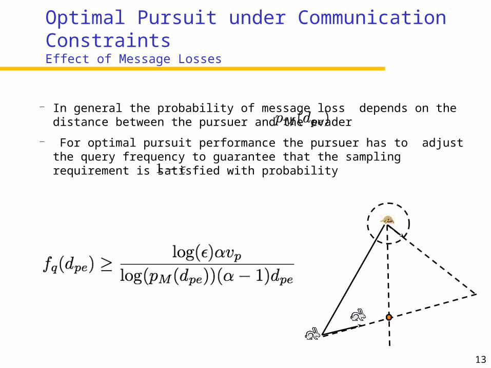
In general the probability of message loss depends on the distance between the pursuer and the evader

For optimal pursuit performance the pursuer has to adjust the query frequency to guarantee that the sampling requirement is satisfied with probability

Optimal Pursuit under Communication ConstraintsEffect of Message Losses

14

• Optimal pursuit-evasion strategies of the perfect information game is the Nash equilibrium of the game with delayed information

Optimal Pursuit under Communication ConstraintsNetwork Delays

Trail: network service for tracking

16

Motivating scenario

Mobile Objects tracked by network of static sensors over a large area Network runs a tracking service Application (residing on mobile objects) issues query of the

form “Find object X” to the tracking service

17

Motivation for Trail

• Queries answered by one (or more) central nodes not scalable

Depletes energy

Increases latency

• One way to make queries local

Publish object state everywhere

But upon every move, global update needed

• Global update for every object move not scalable

• We need to publish object information systematically

18

Informal problem statement

Network tracking service returns query results in time and work proportional to distance from object

Requirement 1: Find distance sensitivity

When an object moves, tracking protocol updates the track in time and work proportional to distance moved

Requirement 2: Update distance sensitivity

19

Trail tracking structure

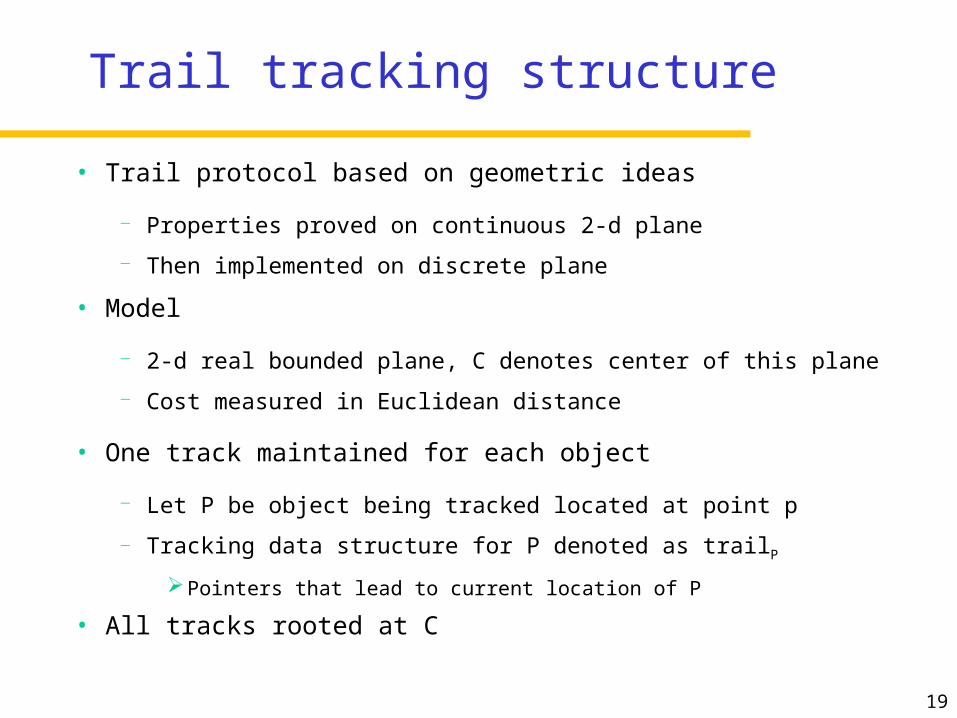
• Trail protocol based on geometric ideas

Properties proved on continuous 2-d plane

Then implemented on discrete plane

• Model

2-d real bounded plane, C denotes center of this plane

Cost measured in Euclidean distance

• One track maintained for each object

Let P be object being tracked located at point p

Tracking data structure for P denoted as trailP

Pointers that lead to current location of P

• All tracks rooted at C

20

Trail intuition

• If trailP restricted to be a straight line, each move will involve update from C

C

p’

p

Instead, trailP marked with vertices on-the-fly Vertices serve as anchor points for update Distance between vertices increases exponentially

moving towards C Anchor updated depending on distance moved After sufficiently large distance, update from C

21

Examples of trailP

C

N3

N2

p

N1

c3

c2

c1

N3

N2

p

N1

c3

c2

c1

C

N3

N2

p

N1

c3

c2

c1

CC

N3

N2

p

N1

c3

c2

c1

N3

N2

N1

c3

c2c1

p

CC

N3

N2

p

N1

c3

c2c1

22

Cost for update and find

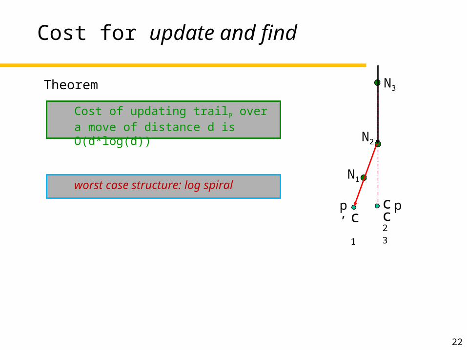
Cost of updating trailP over a move of distance d is O(d*log(d))

Theorem N3

N2

p’

N1

c3

c2

c1

p

worst case structure: log spiral

23

Algorithm for find

Cost of finding P from object Q at point q is O(d) where d is dist(p,q)

Theorem

C

p c2

N3

N2

N1

c3

q

m

Draw successive circles of radii 20, 21, 22 .. 2(log

dist(C,q)) Until trailP is intersected Or reach C

Follow trailP to reach current location of P

Cost includes reaching trailP, following trailP, returning to q

24

Fault-tolerance and adaptivity of Trail

• Fault-tolerance

Nodes may fail after creating trail or old trails may not be deleted

Self-stabilizing actions using heartbeats along trail structure

Tolerating failures during update and find

Route around failures using a method such as left hand rule in GPSR

As size of holes increases, update and find cost proportionally increase

Trail supports graceful degradation

• Adaptivity (Trail yields family of protocols)

Can be tuned based on update and query frequency

When query frequency higher, publish structure increases and find increasingly straight

Extreme case – find is a straight line to C and publish in circles

25

Performance evaluation

• Experimental evaluation (Kansei testbed at OSU)

Used to demonstrate PE tracking application for NEST DARPA project

Intruder tracks collected from Richmond Field Station [140m X 60m]

Tracks injected into Kansei testbed nodes to emulate motion of evaders

15 X 7 node network, 3 ft spacing

3 pursuer 3 evader scenario

Study effect of interference on scaling in

Objects [2 - 10]

Query frequency [0.25 – 1 Hz]

• Simulations [JProwler]

8100 nodes (90 by 90)

Up to 50 objects (uniformly separated and collocated)

Garcia Robots as Pursuers

26

Summary of Trail features

• Trail – a distance sensitive network service

Assumes no hierarchical partitioning of network O(d) find time, cost for object distance d away O(d*log(d)) update time, cost for distance d moved Fault-tolerant

Self-stabilizing, graceful degradation

• When many objects come close together, network interference can cause delay

Synchronized push version? Distance sensitive snapshot service

Distance sensitive snapshot service

A brief overview

28

Informal problem statement

Given

• N nodes, with bounded memory, in f dimensions

• each can sense m-bit information at any time

• each can communicate at W bits per second

Deliver a global snapshot

• at each node (can be relaxed to a subset)

• that uniformly has distance sensitive latency (and distance sensitive resolution, and distance sensitive rate)

State of nearby nodes is fresher

State of nearby nodes more precise

State of nearby nodes refreshed more often

• periodically, as fast as possible (can be relaxed to lower rate)

29

Illustration

30

Illustration

31

Results

Maximum staleness in state of a node i received by a

snapshot at node j is O(log(n) * m * d) where d = dist(i, j)

Resolution of state of a node i in a snapshot received at node

j is Ω(1 / d2) where d = dist(i, j)

Communication cost to deliver a snapshot of one sample

from each node to all nodes is on average O(N * log(n) * m)