tasi2010 nielsen 4 - physics learning laboratories · • only!afrac:on!of! dijet!...

$: TASI2010 Nielsen 4 - Physics Learning Laboratories · • Only!afrac:on!of! dijet! events!are!accepted!by! trigger,!and!we!cannottell! bfrom udsg!in!Level!1!trig! ... FIG. 1: The$
LHC Experiments: Searches for Higgs Bosons

Jason Nielsen Santa Cruz Ins>tute for Par>cle Physics University of California, Santa Cruz

Theore>cal Advanced Studies Ins>tute Boulder, Colorado

June 2010

Standard Model Higgs: What is Known? •  Know couplings to all SM par:cles for a given value of the Higgs boson mass

•  Precision measurements of mW and mt constrain Higgs loop contribu:ons

•  LEP searches rule out mH<114 GeV (strongly)

•  Tevatron searches rule out 163<mH<166 GeV

80.3

80.4

80.5

150 175 200

mH !GeV"114 300 1000

mt !GeV"

mW

!G

eV"

68# CL

LEP1 and SLDLEP2 and Tevatron (prel.)

August 2009

J.Nielsen TASI 2010 2

Higgs Produc:on Mechanisms at LHC


Kunszt et al.

Branching Frac:ons for SM Higgs 1

0.1

10-2

10-3

bb_

WW

!! gg ZZ

cc_

Z"""

120 140 160 180 200100mH (GeV/c2)

SM Higgs branching ratios (HDECAY)


•  Fixed par:al widths found in textbooks, but the frac:on of the total width changes quickly with mH as phase space for new decay channels opens

•  Note ra:o of WW to ZZ, as required by Lagrangian term

L ! (2M2W HW

+µ W

!µ

+M2ZHZµZ

µ)Plot by J. Conway

General Overview of Search Strategy •  We look not only for a discrepancy with respect to (non-‐Higgs) SM, but also consistency with Higgs produc:on

•  Choose specific signature of Higgs produc:on (“channel”) •  Develop event selec:on to reject backgrounds from physics processes and mismeasurements in the signature

•  Es:mate the contribu:on to the data sample from background events and puta:ve signal event – Goal is to measure the contribu:ons directly from data to avoid theore:cal bias or simula:on bias

•  Quan:fy the probability observed dataset is consistent with the background+signal or background-‐only


Sta:s:cs Interlude: Poisson Distribu:on •  Suppose we expect 40 background (SM) events and have a model that predicts 10 new physics signal events

•  Employ Central Limit Theorem by thinking of our experiment as one of many possible experiments:


•  If we observe 40 events, can we exclude the model?

•  If we observe 50 events, can we exclude the Standard Model?

•  60 events?

Entries 10000Mean 39.92RMS 6.395

Total number of observed events0 10 20 30 40 50 60 70 800

50

100

150

200

250

Entries 10000Mean 39.92RMS 6.395

40 Background Events

“Number of Sigma” Discrepancies

•  “Sigma” is ogen a shorthand reflec:ng probability for dataset to represent SM, instead of other way around

•  Be aware of one-‐sided vs. two-‐sided defini:ons of α when comparing parameter measurements and number-‐coun:ng experiments


32. Statistics 23

Table 32.1: Area of the tails ! outside ±" from the mean of a Gaussiandistribution.

! " ! "

0.3173 1# 0.2 1.28#

4.55 !10!2 2# 0.1 1.64#

2.7 !10!3 3# 0.05 1.96#

6.3!10!5 4# 0.01 2.58#

5.7!10!7 5# 0.001 3.29#

2.0!10!9 6# 10!4 3.89#

The relation (32.53) can be re-expressed using the cumulative distribution function forthe $2 distribution as

! = 1 " F ($2; n) , (32.54)

for $2 = ("/#)2 and n = 1 degree of freedom. This can be obtained from Fig. 32.1 on then = 1 curve or by using the CERNLIB routine PROB or the ROOT function TMath::Prob.

For multivariate measurements of, say, n parameter estimates !! = (!%1, . . . , !%n), onerequires the full covariance matrix Vij = cov[!%i, !%j ], which can be estimated as describedin Sections 32.1.2 and 32.1.3. Under fairly general conditions with the methods ofmaximum-likelihood or least-squares in the large sample limit, the estimators will bedistributed according to a multivariate Gaussian centered about the true (unknown)values !, and furthermore, the likelihood function itself takes on a Gaussian shape.

The standard error ellipse for the pair (!%i, !%j) is shown in Fig. 32.5, correspondingto a contour $2 = $2

min + 1 or ln L = lnLmax " 1/2. The ellipse is centered about theestimated values !!, and the tangents to the ellipse give the standard deviations of theestimators, #i and #j . The angle of the major axis of the ellipse is given by

tan 2& =2'ij#i#j

#2j " #2

i

, (32.55)

where 'ij = cov[!%i, !%j ]/#i#j is the correlation coe!cient.The correlation coe!cient can be visualized as the fraction of the distance #i from the

ellipse’s horizontal centerline at which the ellipse becomes tangent to vertical, i.e., at thedistance 'ij#i below the centerline as shown. As 'ij goes to +1 or "1, the ellipse thinsto a diagonal line.

It could happen that one of the parameters, say, %j , is known from previousmeasurements to a precision much better than #j , so that the current measurementcontributes almost nothing to the knowledge of %j . However, the current measurement of%i and its dependence on %j may still be important. In this case, instead of quoting bothparameter estimates and their correlation, one sometimes reports the value of %i, which

January 28, 2010 12:02

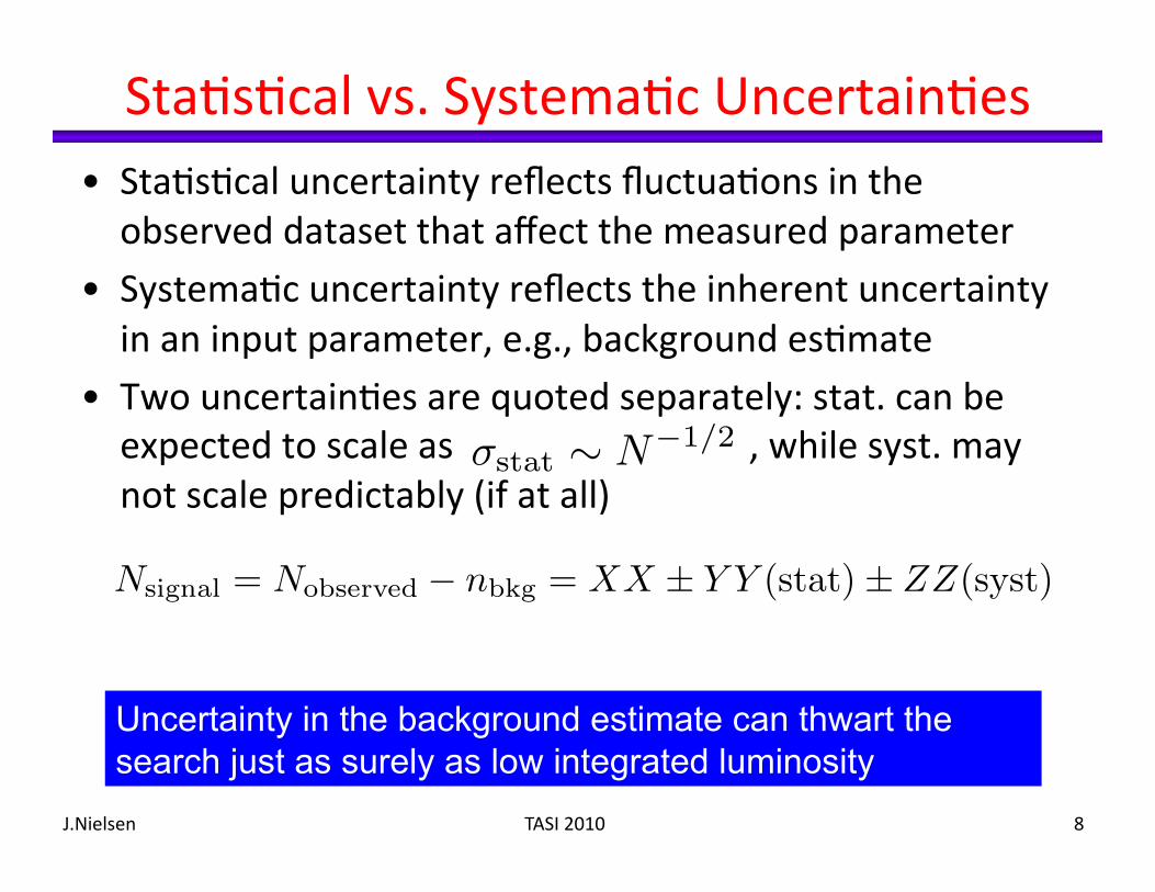
Sta:s:cal vs. Systema:c Uncertain:es •  Sta:s:cal uncertainty reflects fluctua:ons in the observed dataset that affect the measured parameter

•  Systema:c uncertainty reflects the inherent uncertainty in an input parameter, e.g., background es:mate

•  Two uncertain:es are quoted separately: stat. can be expected to scale as , while syst. may not scale predictably (if at all)


!stat ! N!1/2

Uncertainty in the background estimate can thwart the search just as surely as low integrated luminosity

Nsignal = Nobserved ! nbkg = XX ± Y Y (stat) ± ZZ(syst)

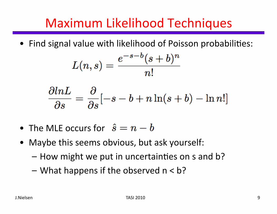
Maximum Likelihood Techniques •  Find signal value with likelihood of Poisson probabili:es:

•  The MLE occurs for

•  Maybe this seems obvious, but ask yourself: – How might we put in uncertain:es on s and b? – What happens if the observed n < b?


Binned Likelihood Techniques


Binned likelihood works in the same way as unbinned likelihood, but the probability treats bins and their contents instead of individual data points

Some informa:on is lost due to the bin widths; OK as long as the bin widths are much narrower than any features

Uncertain:es on Likelihood Parameters •  Again, when N is large, the likelihood becomes Gaussian

•  The Taylor expansion gives

•  Iden:fy Δα2 as

•  Now if we write –  Then

•  Each unit of 2 ln L is taken to be “1 sigma,” in the spirit of our table rela:ng probability and Gaussian “sigma”


Hypothesis Tes:ng •  Typically we are interested in tes:ng two hypotheses:

–  background-‐only produc:on (s=0) –  signal+background produc:on (s>0)

•  If the data favor the laqer hypothesis and strongly disfavor the former, then we have a discovery!

•  Construct a likelihood ra:o: how ogen can certain value can be expected from experiment in presence of signal?

–  For a discovery, we usually talk about excluding the background hypothesis at >5σ. This is Pb<10-‐7

–  For “evidence,” the standard is lower: just 3σ


Search for H→ZZ •  Usual clean signature for Z decay to leptons (e/µ); require lepton pairs have invariant mass near mΖ

•  Produc:on details are not important since signature is so clean; background is just ZZ!

•  “Golden” channel for high-‐mass Higgs searches


ATLAS CSC Book

mH=180 mH=300

Search for H→γγ


CMS, 1 fb-1 @ 14 TeV

Search for H→ττ

•  Branching frac:on for is roughly 10% •  Select 2 τ candidates: both leptonic or leptonic+hadronic •  Measure MET to es:mate total energy taken by all ν’s •  Use kinema:c reconstruc:on trick (τ momentum is approximately the ν momentum) to appor:on the MET


mH ! 2mW

•  May be necessary to include other produc:on mechanisms like vector boson fusion (VBF) for cleaner signature

Search for H→WW •  Pros: rate is large, decay to leptons is clean •  Cons: 2 high-‐ET neutrinos mean no invariant mass peak •  S:ll possible if the enhanced rate of can be combined with change in distribu:ons


2!+ !ET

•  Direct WW produc:on and top quark pairs have similar signatures

•  No need to veto on Drell-‐Yan produc:on if the mass distribu:on is included

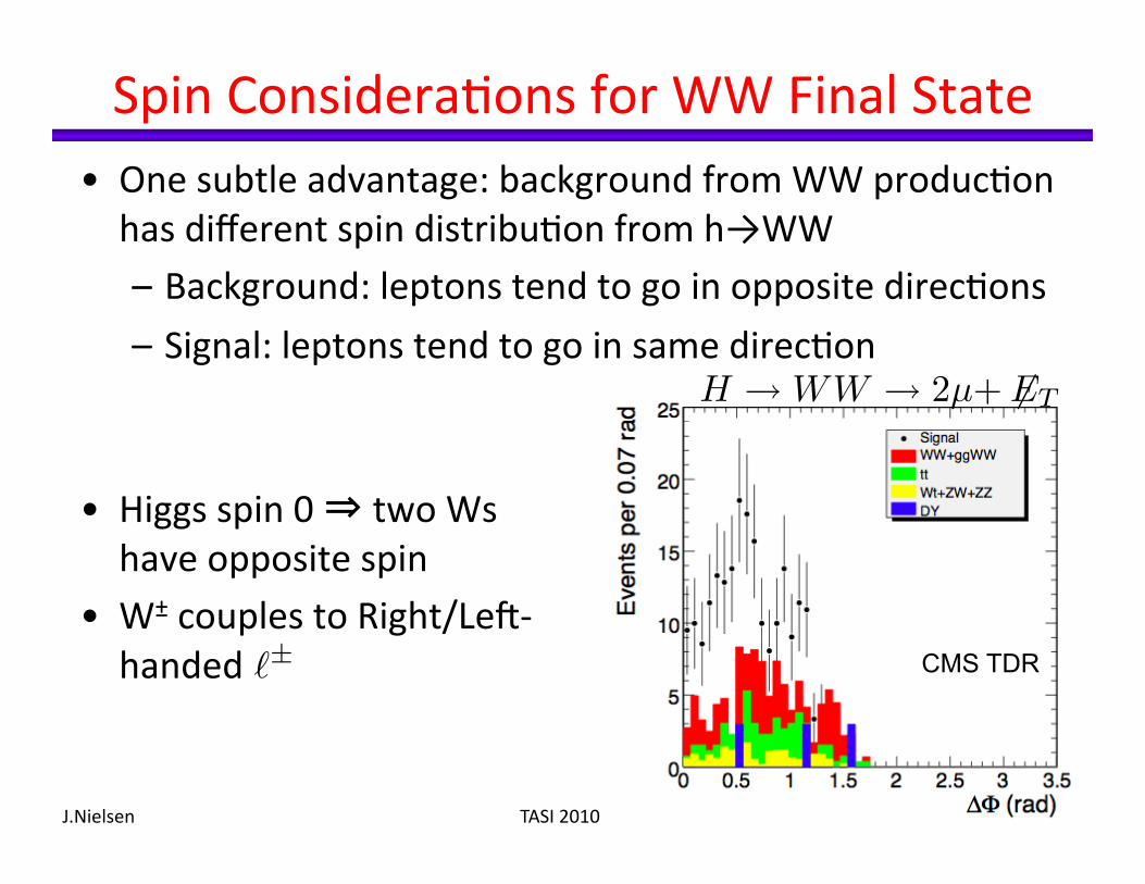
Spin Considera:ons for WW Final State •  One subtle advantage: background from WW produc:on has different spin distribu:on from h→WW –  Background: leptons tend to go in opposite direc:ons –  Signal: leptons tend to go in same direc:on


!±

•  Higgs spin 0 ⇒ two Ws have opposite spin

•  W± couples to Right/Leg-‐handed CMS TDR

H ! WW ! 2µ+ "ET

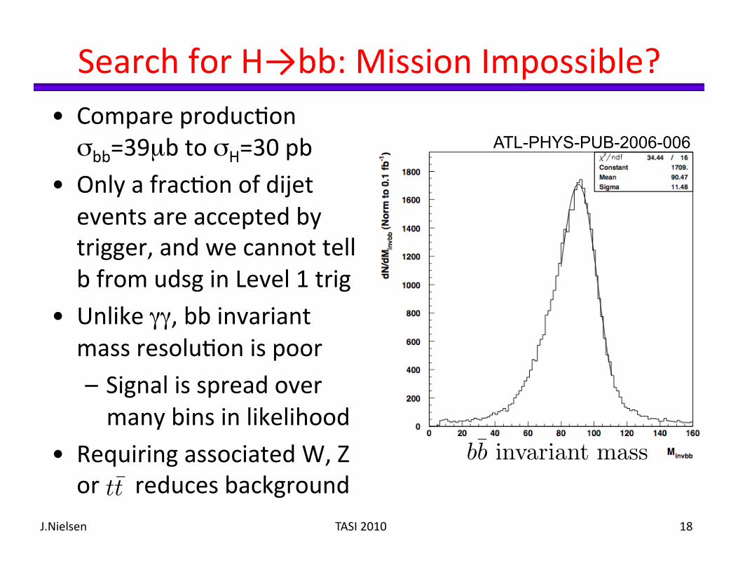
Search for H→bb: Mission Impossible? •  Compare produc:on σbb=39µb to σH=30 pb

•  Only a frac:on of dijet events are accepted by trigger, and we cannot tell b from udsg in Level 1 trig

•  Unlike γγ, bb invariant mass resolu:on is poor –  Signal is spread over many bins in likelihood

•  Requiring associated W, Z or reduces background


bb̄ invariant mass

ATL-PHYS-PUB-2006-006

tt̄

Finding Higgs in Boosted Jets •  Restrict the WH/ZH search to region of phase space in which vector boson has large transverse momentum: system is boosted into a single fat jet

– High-‐mass jet substructure is nearly unique to Higgs decay, so background is reduced


2

b Rbb Rfilt

Rbbg

bR

mass drop filter

FIG. 1: The three stages of our jet analysis: starting from a hard massive jet on angular scale R, one identifies the Higgsneighbourhood within it by undoing the clustering (e!ectively shrinking the jet radius) until the jet splits into two subjetseach with a significantly lower mass; within this region one then further reduces the radius to Rfilt and takes the three hardestsubjets, so as to filter away UE contamination while retaining hard perturbative radiation from the Higgs decay products.

objects (particles) i and j, recombines the closest pair,updates the set of distances and repeats the procedureuntil all objects are separated by a !Rij > R, where Ris a parameter of the algorithm. It provides a hierarchicalstructure for the clustering, like the K!algorithm [9, 10],but in angles rather than in relative transverse momenta(both are implemented in FastJet 2.3[11]).

Given a hard jet j, obtained with some radius R, wethen use the following new iterative decomposition proce-dure to search for a generic boosted heavy-particle decay.It involves two dimensionless parameters, µ and ycut:

1. Break the jet j into two subjets by undoing its laststage of clustering. Label the two subjets j1, j2 suchthat mj1 > mj2 .

2. If there was a significant mass drop (MD), mj1 <µmj, and the splitting is not too asymmetric, y =min(p2

tj1,p2

tj2)

m2

j

!R2j1,j2

> ycut, then deem j to be the

heavy-particle neighbourhood and exit the loop.Note that y ! min(ptj1 , ptj2)/ max(ptj1 , ptj2).

1

3. Otherwise redefine j to be equal to j1 and go backto step 1.

The final jet j is to be considered as the candidate Higgsboson if both j1 and j2 have b tags. One can then identifyRbb̄ with !Rj1j2 . The e"ective size of jet j will thus bejust su#cient to contain the QCD radiation from theHiggs decay, which, because of angular ordering [12, 13,14], will almost entirely be emitted in the two angularcones of size Rbb̄ around the b quarks.

The two parameters µ and ycut may be chosen inde-pendently of the Higgs mass and pT . Taking µ ! 1/

"3

ensures that if, in its rest frame, the Higgs decays to aMercedes bb̄g configuration, then it will still trigger themass drop condition (we actually take µ = 0.67). The cuton y ! min(zj1 , zj2)/ max(zj1 , zj2) eliminates the asym-metric configurations that most commonly generate sig-nificant jet masses in non-b or single-b jets, due to the

1 Note also that this ycut is related to, but not the same as, thatused to calculate the splitting scale in [5, 6], which takes the jetpT as the reference scale rather than the jet mass.

Jet definition !S/fb !B/fb S/!

B · fb

C/A, R = 1.2, MD-F 0.57 0.51 0.80

K!, R = 1.0, ycut 0.19 0.74 0.22

SISCone, R = 0.8 0.49 1.33 0.42

TABLE I: Cross section for signal and the Z+jets backgroundin the leptonic Z channel for 200 < pTZ/GeV < 600 and110 < mJ/GeV < 125, with perfect b-tagging; shown forour jet definition, and other standard ones at near optimal Rvalues.

soft gluon divergence. It can be shown that the maxi-mum S/

"B for a Higgs boson compared to mistagged

light jets is to be obtained with ycut ! 0.15. Since wehave mixed tagged and mistagged backgrounds, we use aslightly smaller value, ycut = 0.09.

In practice the above procedure is not yet optimalfor LHC at the transverse momenta of interest, pT #200 $ 300 GeV because, from eq. (1), Rbb̄ ! 2mh/pT isstill quite large and the resulting Higgs mass peak is sub-ject to significant degradation from the underlying event(UE), which scales as R4

bb̄[15]. A second novel element

of our analysis is to filter the Higgs neighbourhood. Thisinvolves resolving it on a finer angular scale, Rfilt < Rbb̄,and taking the three hardest objects (subjets) that ap-pear — thus one captures the dominant O (!s) radiationfrom the Higgs decay, while eliminating much of the UEcontamination. We find Rfilt = min(0.3, Rbb̄/2) to berather e"ective. We also require the two hardest of thesubjets to have the b tags.

The overall procedure is sketched in Fig. 1. We il-lustrate its e"ectiveness by showing in table I (a) thecross section for identified Higgs decays in HZ produc-tion, with mh = 115 GeV and a reconstructed mass re-quired to be in an moderately narrow (but experimen-tally realistic) mass window, and (b) the cross sectionfor background Zbb̄ events in the same mass window.Our results (C/A MD-F) are compared to those for theK!algorithm with the same ycut and the SISCone [16]algorithm based just on the jet mass. The K!algorithmdoes well on background rejection, but su"ers in massresolution, leading to a low signal; SISCone takes in lessUE so gives good resolution on the signal, however, be-cause it ignores the underlying substructure, fares poorlyon background rejection. C/A MD-F performs well both

Butterworth et al. 0802.2470v2

H ! bb̄

gg ! bb̄

Proof of Principle in (W/Z)H→lνbb Channel •  Specific event selec:on

–  pT(V,H) > 300 GeV –  R = 0.7 –  beff/fake = 70%/1%

•  ZZ produc:on is an irreducible background, but also a calibra:on sample with clear peak

•  Basic concepts of jet substructure need to be tested with early data


tasi2010 nielsen 4 - physics learning laboratories · • only!afrac:on!of! dijet!...

Documents