tax compliance under tax regime changes · by monetary considerations. other considerations and...

Tax compliance under tax regime changes*

Friedrich Heinemann and Martin G. Kocher

Abstract: In this paper we focus on the compliance effects of tax regime changes.

According to the economic model of tax evasion, a tax reform should affect compliance

through its impact on tax rates and incentives. Our findings demonstrate the importance of

at least two further effects not covered by the traditional model: First, reform losers tend to

evade more taxes after the reform. Second, a reform from a proportionate towards a

progressive system decreases compliance compared to a switch in the reverse direction.

Interestingly, however, the level of compliance is generally higher under a progressive than

under a proportionate regime.

20 February 2009

JEL classification: C72, C91, H26

Keywords: tax reforms, tax compliance, experiment

Friedrich Heinemann Center for European Economic Research (ZEW) L7, 1 D-68161 Mannheim Germany [email protected]

Martin G. Kocher Department of Economics University of Munich Geschwister-Scholl-Platz 1 D-80539 Munich Germany [email protected]

* Kocher gratefully acknowledges financial support by the Munich Experimental Laboratory for

Economics and Social Sciences (MELESSA). We thank seminar participants in Munich for helpful

comments on the design of the experiment and Julius Pahlke for excellent research assistance.

1

1 Introduction Economists typically discuss tax regime changes or tax reforms under aspects of

economic incentives and efficiency regarding labor supply, investment as well as savings

decisions and similar issues. A potentially important incentive effect of tax reforms which

has largely been neglected so far is the interest of this paper: the impact of a tax regime

changes on the inclination or willingness of tax payers to comply with tax rules.

Our contribution can be based on the far advanced theoretical and empirical

literature on tax compliance. This literature continues to be inspired by the striking contrast

between high observable tax compliance and low compliance predicted by the economic

model of tax compliance (Allingham and Sandmo, 1972) for a realistic degree of risk

aversion. This does not only hold for studies based on survey or field data but also for

experimental studies where “in most cases the level of tax compliance was higher than

predicted” (Torgler, 2002, p. 677).

In the course of the last two decades important explanations have emerged which

contribute to understand this contrast (for a more complete coverage of the literature see

Kirchler, 2007, Torgler, 2002, and Andreoni, 1998): Individuals tend to overweight the

probability of an audit (Alm, McClelland and Schulze, 1992). The perception that tax

payments are linked to the financing of beneficial public goods fosters compliance (Alm,

Jackson at McKee, 1992). Feld and Frey (2002, 2007) interpret the interaction of taxpayers

and tax authorities in the context of a reciprocal “psychological contract” which effectively

binds taxpayers if their political participation rights are developed and if they are friendly

treated by tax authorities. In line with the view of tax payments as reciprocal behavior is

the finding that the perceived equity of a tax system influences compliance rates (the

starting point of this line of research was Spicer and Becker, 1980; for subsequent

experimental studies see Torgler, 2002). Further attempts to explain the tax compliance

puzzle point to the role of social norms or social preferences, which can affect the tax

compliance decision. Social norms on tax compliance (or “tax morale”) may explain

different compliance experiences for countries with similar fiscal systems (Alm, Sanchez

and De Juan, 1995). Tax morale itself is dependent on institutions. E.g., Torgler (2005)

establishes a positive impact of Swiss direct democracy on tax morale. Recently,

Maciejovsky, Kirchler and Schwarzenberger (2007) have put emphasis on the dynamic

dimension of tax compliance in an experimental setting which explores the effects of

audits over time.

2

We follow the latter authors in the respect that we focus on the dynamics of tax

compliance, too. However, our context is that of tax reform. As far as we know, we are the

first to investigate compliance effects of tax regimes switches experimentally. We

implement this through fully incentivized, individual decisions on tax compliance in the

experimental laboratory. More specifically, our study focuses on the impact of a reform

from a progressive towards a proportionate tax tariff and vice versa on individual tax

compliance. Furthermore, our study is novel by analyzing the behavioral determinants of

individual choices regarding the preferred tax regime after participants have experienced

both regimes. A further innovative feature of our empirical approach is that the taxable

income in the experiment depends on individual achievements (see also Anderhub et al.,

2001). This feature induces stronger entitlements over the taxable income and increases the

external validity of our experimental setup.

Our empirical results corroborate the view that compliance is affected by regime

changes beyond the predictions of the traditional economic model of tax evasion. A change

from a progressive to a proportionate system is significantly more beneficial in terms of

tax compliance than a switch in the reverse direction. This result hints to the importance of

the pre-reform point of reference in the individual compliance decision. Furthermore,

reform losers tend to evade taxes to a greater extent after the reform compared to reform

winners. The preference for one of the two systems on the individual is strongly influenced

by monetary considerations. Other considerations and individual characteristics play a

minor role in shaping this preference.

Changes to the degree of a tax system’s progressiveness are a key element of many

tax reforms introduced or debated. For decades, income tax reforms in industrial countries

have been characterized by a combination of base broadening and cuts in tax rates (OECD,

2006). An even more radical approach is the introduction of flat tax regimes, which are

highly heterogeneous in reality but share the common feature of a single marginal tax rate

for incomes above a tax free allowance. Flat tax reforms have received increasing interest

resulting from their popularity among Eastern European countries (Keen, Kim and

Varasano, 2008). Proponents claim that their simplicity and incentives raise compliance.

Indeed, on the basis of household panel data, Ivanova, Keen and Klemm (2005) report that

the Russian flat tax reform from 2001 has been associated with a higher degree of

compliance.

3

However, natural experiments do not allow for an unambiguous identification of the

driving forces behind tax compliance because it is next to impossible to disentangle several

competing explanations. Relevant variables such as the tax tariff, changes in the

effectiveness of the tax administration and the general social and economic environment

change concurrently. Moreover, the impact of reforms on compliance cannot be measured

precisely from field data or surveys because of the secret nature of tax evasion. Controlled

laboratory experiments also have their weak points but they allow for a much finer-tuned

assessment of behavioral incentive effects, because they allow sustaining control over all

important determinants of decisions and, more importantly, causally ascribing changes of

behavior to exogenous treatment variations. Hence, often the combination of both

empirical results from the laboratory and results based on field data permits drawing

definite conclusions that are valuable for policy makers.

The merits of laboratory experiments on tax compliance decisions as a complement

to field or survey studies has recently increased the number of experimental papers in that

area quite rapidly. Existing contributions, which we survey briefly in the next section, have

substantiated diverse factors impacting on compliance ranging from tax rates, the

frequency of audits, the size and structure of fines over social norms and cultural factors to

institutional factors related, e.g., to fiscal decentralization. They serve as an important

starting point for our study, even though they have not yet dealt with the impact of a tax

regime change on compliance.

Our paper is structured as follows: After deriving our theoretical expectations on the

impact of tax reform on compliance (in section 2) we present our experimental design in

section 3. Section 4 contains the results, and section 5 concludes the paper.

4

2 Tax regimes and tax compliance: Theoretical

expectations The brief literature review above has clarified that the economic model of tax

compliance is not sufficient to explain the extent of honest tax declaration. Hence, studying

the impact of tax reform on compliance must allow for at least two kinds of effects. First,

according to the logic of the economic model, a tax reform should influence compliance if

it involves changes of tax rates, the level and construction of fines or variations of audit

probabilities. Second, a tax regime change may have effects on compliance because it

influences compliance norms or the perceived fairness of a tax regime where the latter may

be influence by individual gains or losses from the reform.

Tax reform effects in the economic model of tax compliance

The seminal paper which has inspired the broad theoretical and empirical literature

studying the driving forces behind tax compliance is Allingham and Sandmo (1972,

henceforth: AS). In the AS-model tax cheating is regarded as an investment into a risky

asset. By hiding a certain fraction of income tax payers embark on a lottery with two

possible outcomes: Either they are not caught and “earn” the tax on the income not

declared or they are audited and lose the fine. Key parameters that according to the AS-

model should drive tax compliance are the fine rate, the audit probability, the tax rate, the

level of income and individual risk preferences. Ceteris paribus, investment into tax

cheating will be the larger, the lower the risk of detection (determined by the audit system

and the audit probability), the lower the potential loss (determined by the construction and

the size of the fine), the higher the potential return (determined by the tax rate) and the

lower individual risk aversion (which is usually negatively correlated to income).

Since changes in tax rates are a defining characteristic of tax regime reforms, it is

particularly important to understand the incentive effects of a variation in the income tax

rate (Andreoni, Erard and Feinstein, 1998). In the original AS-model, the fine is

constructed to be proportionate to the income evaded. Under this assumption raising the

tax rate has an ambiguous effect on compliance. On the one hand, it lowers net income

which should make people more risk averse under the standard assumption of absolute risk

aversion falling with income. On the other hand, a higher tax rate increases the returns to

cheating without increasing the size of the fine, since the latter depends on the income

5

evaded. By contrast, the effect is unambiguous if the fine is proportionate to the tax evaded

(Yitzhaki, 1974): The income effect and the substitution effect now both work towards

more compliance with an increasing tax rate. With the Yitzhaki-type of fine we would

expect tax compliance to increase (decrease) if a tax reform increases (decreases) the tax

rate.

Tax reform effects beyond the economic model

A tax reform may impact on compliance beyond its pure incentive effects linked to

changing parameters of the tax system. Here, the finding of the tax compliance literature

(see above) according to which tax compliance is supported by reciprocity and the

perception of the tax system’s fairness, is relevant. A new tax regime change offers a direct

comparison between two systems and may lead to a reassessment of the system’s fairness

with consequences for compliance. In this regard, it is relevant that the perceived fairness

of a tax regime is closely linked to self-interest: Based on a survey of US citizens, Bobek

and Hatfield (2001) show that the perceived fairness of the introduction of a flat tax is

driven by the individual gains or losses pointing to the relevance of a self-serving bias also

in the context of assessments of tax regime changes. The essence of the self-serving bias is

“to conflate what is fair with what benefits oneself” (Babcock and Lowenstein, 1997, p.

110). From these considerations we derive the following prediction: Beyond the impact

associated with changing tax parameters, tax reform impacts on compliance if the regime

change affects the perceived fairness of the tax system. Part of this perceptional effect will

be connected to individual losses and gains from the regime change where losses (gains)

will be associated with less (more) compliance.1

1 This hypothesis not only rests on a possible self-serving bias and the corresponding fairness

judgments but can also be explained by the motive of “loss repair”: Andreoni, Erard and Feinstein (1998)

explain the unexpectedly negative effect of audit on compliance with the intention to get back some of the

money foregone after a fine. In analogy, a tax reform confronting the individual tax payer with losses should

lead to more evasion motivated by a compensation strategy.

6

3 Model and experimental design Our experimental design extends the standard experimental approach to study tax

compliance decisions in at least three respects. First, we model individual expected income

to depend on individual achievements in order to induce stronger entitlements over the

taxable income. Second, individuals experience a fundamental tax regime change from a

proportionate towards a progressive system and vice versa. And third, subsequent to the

experience of both tax regimes, participants can choose their preferred tax regime and

decide about compliance in final period with strongly increased monetary incentives.

In our experimental setup the incomes of Ii∈ individuals in period t, Yi,t, is

distributed over the closed interval [0,2000]. The expected income E[Y] of the population

is equal to 1000 but the individual probability distribution is dependent on an individual

characteristic ]1,0[∈ie that is an indicator for relative ability to earn income. Each

individual is assigned this parameter in a way such that the relatively best-performing

individual is assigned ei = 1 and the least-performing individual ei = 0. If n is the number

of individuals in the economy, 1/(n – 1) is the difference between two adjacent e-values.

The parameter ei can be interpreted as a general, time-independent personal pre-disposition

for the ability to earn income with 0/][ >∂∂ ieYE .

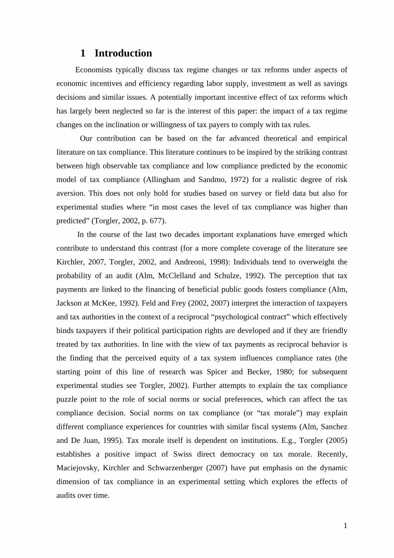
Figure 1: Probability distribution of income for an economy with 20 individuals

0

0.0001

0.0002

0.0003

0.0004

0.0005

0.0006

0.0007

0.0008

0.0009

020

040

060

080

010

0012

0014

0016

0018

0020

00

Income

Prob

abili

ties

e=0 e=0.21 e=0.53 e=0.79 e=1

7

More specifically, an ei > 0.5 shifts the expected value of individual income in a

given period E[Yi,t] to the right, and an ei < 0.5 shifts the expected value of individual

income E[Yi,t] to the left of the median income while, however, leaving the population

expected income unchanged.2 In the experiment, the individual probability distribution

over income is normally distributed with X = N (μi ; σ2) = N (μi ; 5002) with cut-offs at 0

and 2000, and ei is proportional to μi, i.e. ii e2000=μ . Figure 1 shows the distributions for

e=0, e=0.21, e=0.53, e=0.79 and e=1 for the purpose of illustration.

Table 1: Overview of tax regimes

Progressive tax regime Proportionate tax regime

Income Average tax rate Tax amount Average tax rate Tax amount 0 0.00 0.00 0.25 0.00

100 0.00 0.00 0.25 25.00 200 0.00 0.00 0.25 50.00 300 0.00 0.00 0.25 75.00 400 0.00 0.00 0.25 100.00 500 0.00 0.00 0.25 125.00 600 0.016 9.72 0.25 150.00 700 0.046 32.34 0.25 175.00 800 0.076 60.96 0.25 200.00 900 0.106 95.58 0.25 225.00

1000 0.136 136.20 0.25 250.00 1100 0.166 182.82 0.25 275.00 1200 0.196 235.44 0.25 300.00 1300 0.226 294.06 0.25 325.00 1400 0.256 358.68 0.25 350.00 1500 0.286 429.30 0.25 375.00 1600 0.316 505.92 0.25 400.00 1700 0.346 588.54 0.25 425.00 1800 0.376 677.16 0.25 450.00 1900 0.406 771.78 0.25 475.00 2000 0.436 872.40 0.25 500.00

In each period { }Rr ..., ,2 ,1∈ individuals learn their actual income and have to

declare an amount riri YD ,,0 ≤≤ . Di,r is taxed according to a tax function Ti,r that can take

on two forms (the two tax regimes): (i) either being proportionate with ripropri DtT ,, *= , or

(ii) being progressive with fgDDtT ririprogri

/)( ,,,−= if gD ri ≥, and 0 otherwise, where t

2 This is an important feature when introducing a tax regime change, because it allows us to directly

compare the two regimes.

8

denotes the tax rate, g is the tax-free income and f is a parameter that determines at which

income the maximum marginal tax rate kicks in.3 Table 1 displays the tax function. Note

that the expected revenues of the two tax regimes are identical.4

Tax jurisdictions are formed out of 1 < m < n individuals, and tax revenues within a

jurisdiction (i.e., ∑=

m

i riD1 , ) are divided equally among the m individuals each period. A tax

audit take place with a commonly known probability p, and failing to comply with Di,r =

Yi,r in the audit leads to a fine s, with )]()([ ,,,,, ririririri DTYTqs −= , i.e. q times the evaded

tax in this period. Thus, we have implemented the Yitzhaki (1974) type of fine which

safeguards that the expected effect of a tax rate increase has an unambiguously positive

effect on compliance (see above). Fines are forfeit and are not redistributed within the

jurisdiction. Tax evasions that are not detected do not bear any consequences.

Thus, a player i faces the following payoff function in a single period (suppressing

the time index):

])()[1(})]()([)({ 11

m

DDTYp

m

DDTYTqDTYp

m

jj

ii

m

jj

iiiiiii

∑∑== +−−++−−−=π (1)

In the experiment we choose the following parameters: size of the jurisdiction m = 2,

size of the economy n = 10, audit probability p = 0.155, the fine rate q = 3, the tax function

parameters g = 546, f = 1,500, the proportionate tax rate t* = 0.25, and the top marginal tax

rate of the progressive tax t = 0.45. It is easy to show for both of our tax regimes – the

3 For reasons of parsimony and analytical clarity we chose very easy tax regimes. Moreover,

straightforward tax formulae make it much easier for subjects to understand their task. Since we never

intended to exactly copy real-world tax regimes, we will not interpret the absolute level of tax compliance.

Our focus is on the causal effects of our treatment variations. For the latter, clear incentive effects facilitate

inferences on behavioral consequences of tax regime switches. 4 Note that our experimental program induced the expected income E[Y] of the population to be

slightly skewed to the right and, hence, the expected revenues of the two tax regimes were not identical in the

experiment. All our results and conclusions are unaffected by this feature. We will return to this issue in the

results section. 5 Like in many other experiments, we choose an auditing probability that is considerably higher than

the one in the real world. This is to account for the fact that several real-world leveraging effects of auditing

such as potential social disapproval after being caught cheating or increased auditing scrutiny after once

being caught cheating are not separately modeled in our experiment.

9

progressive and the proportionate tax – that risk-neutral money-maximizing individuals

would always declare Di,t = 0.

As already mentioned, entitlement over money is strengthened by making the

individual ability-to-earn-money parameter ei dependent on the individual performance in

a quiz at the beginning of the experiment. The quiz contained 20 trivia questions (which

can be found in Appendix B). Each of them offered four possible answers of which only

one was correct. Subjects learned that their endowment in later parts of the experiment will

depend on their performance in the quiz, and they learned in the instructions (see Appendix

A) for the tax game that per-period income contains a stochastic component, but they did

not learn in what exact way income was determined. Specifically, in the instructions there

was no reference to the tournament-like or relative nature in which ei was determined.

Each of our four experimental sessions followed the protocol described below. 20

subjects were welcomed to the laboratory and received written instructions for the trivia

quiz (part one in the instructions) and the first part (part two in the instructions) of the tax

game (either under the progressive tax regime in two sessions or under the proportionate

tax regime in the other two sessions).6 At this stage, participants only knew that there

would be further parts of the experiments but had no idea on their contents. The

instructions were read aloud, and we gave plenty of time to ask private questions before we

started the experiment.

Upon completion of the second part of the experiment, subjects received written

instruction that were again read aloud for part three of the experiment (the tax game under

a progressive tax regime or under a proportionate tax regime). Hence, we implemented a

within-subject design. Both tax game parts (periods r1-r10 and periods r11-r20) lasted for 10

periods each, and this was common knowledge at the beginning of each part. Before the

final period r = 21 (denoted part four in the instructions), subjects in the experiment are

asked which tax regime they prefer, and this regime is, then, implemented for the final

period for the individual decision-maker. Monetary incentives for this final period were

five times higher than for a period in the previous parts in order to make the self-selection

into the preferred regime highly salient. Each period subjects were paired (remember, m =

2) randomly in a stranger design (this was common knowledge) in matching groups of size

6 Providing subjects with instructions for the first two parts right away helps to make the claim that

later endowments depend on the performance in the quiz more credible.

10

10 for obtaining one statistically independent observation. At the end of each experimental

session, subjects went through a risk test (Holt and Laury, 2002) and were asked to answer

several attitudinal (tax morale) and personal (socio-economic variables) survey questions.

The experiment was run with the help of z-tree (Fischbacher, 2007). In total, we had

80 participants (students with a variety of majors) in four sessions, each of them lasting

less than two hours. Subjects earned € 24.15 on average. During the experiment, earnings

were framed in experimental points with a pre-announced exchange rate of experimental

points into euro. Sessions ended with private, in-cash payment.

4 Experimental results We first present a short overview of the main descriptive results of our experiment

(section 5.1). Section 5.2 investigates the driving forces behind compliance, and section

5.3 analyzes the determinants of the endogenous choice of the tax regime.7

4.1 Overview of main descriptive results In the following, our discussion will mainly focus on the impact of the tax regime

switch, because our general results on tax compliance are in line with the existing

experimental literature.

Figure 2: Tax compliance under the two regimes

Tax honesty

00.10.20.30.40.50.60.7

1 2 3 4 5 6 7 8 9 10

Period

aver

age

% d

ecla

red

Progressive Proportional

7 The raw data from our experiment can be found in Appendix C.

11

Figure 2 provides average results on tax compliance under the two regimes. It

shows that under the progressive tax regime, the average percentage of declared income

stays quite stable around 0.60, whereas it drops from 0.55 in the first period to below 0.40

in the final period of the proportionate regime. Note that we pool data in Figure 2,

regardless of whether subjects experienced the progressive scheme or the proportionate

scheme first. The average percentage of compliance in the progressive treatment (0.59) is

significantly higher than the average percentage of compliance in the proportionate

treatment (0.45) (Wilcoxon-signed ranks test; p = 0.025; N = 88).

Figure 3 allows for a more disaggregated view on the effects of tax regime

switches. The sessions that started with the progressive scheme exhibit a very high level of

tax honesty in the initial periods which, however, decays over time. The introduction of the

proportionate scheme leads to a drop of about ten percentage points in average compliance.

In contrast, the average compliance is much lower in the sessions that started with the

proportionate scheme. The nature of the decay, however, is very similar to the sessions

with the reverse order, albeit on a much lower level of compliance. The introduction of the

progressive tax regime after period 10 increases average tax compliance by about ten

percentage points. Of course, this descriptive view does not allow to distinguish between

the different reform effects which originate from altering incentives through chaning tax

rates on the one hand and the change in the tax regime as such.

8 Note that this is a very conservative test on the level of matching group averages. On the individual

level, the difference is highly significant (p < 0.001).

12

Figure 3: Effects of the regime change

Tax regime change

00.10.20.30.40.50.60.70.80.9

1 2 3 4 5 6 7 8 9 10 11 12 13 14 15 16 17 18 19 20

Period

% d

ecla

red

Prog-Prop Prop-Prog

Figure 4: Distributional histograms of compliance

Panel A: Progressive tax regime Panel B: Proportionate tax regime

010

2030

40Pe

rce

nt

0 .2 .4 .6 .8 1progressive

05

1015

20Pe

rce

nt

0 .2 .4 .6 .8 1proportionate

Neither do average results properly reflect the fact that there is quite some

individual heterogeneity in tax compliance. We observe both subjects that always report

their true income and subjects that always report zero income. Subjects also declare

amounts below their true income but above zero, and quite a few subjects change their

compliance behavior over the course of the experiment contingent on audits. Figure 4

provides distributional histograms of compliance under the two regimes. It is immediately

obvious that tax evasion is much higher under the proportionate system.

13

4.2 Econometric analysis compliance Our econometric approach for the explanation of the share of total income declared

reflects the preceding theoretical consideration. Hence, the estimation model includes a full

set of variables related to incentives in the light of the AS model and some further control

variables of importance in the light of the experimental tax compliance literature. But, in

addition, we also take account of possible effects related to the individual experience with

the tax regime change.

Given the censored dependent variable we apply a Tobit regression employing

Huber-White standard errors. Column (1) in Table 2 presents the baseline regression.

Income, risk aversion (identified form the risk test according to Holt and Laury, 2002) and

the marginal tax rate are the control variables corresponding to the AS model. We also

include a number of control variables whose importance has been repeatedly demonstrated

in the experimental literature: A dummy for a fine in the last period, a period index and a

gender dummy. Although the audit probability is common knowledge in experimental

design and should not affect compliance of rational agents it is well known from the

literature that a preceding fine tends to lower subsequent compliance. This is explained by

both a misperception of chance and, to a weaker extent, a tendency of subjects to “repair

their losses” from a preceding fine (Maciejovsky, Krichler and Schwarzenberger, 2007).

The repetition of tax compliance games also matters for compliance. The degree of tax

evasion decays over time during a series of repeated declarations. Concerning the impact

of gender, females have been identified to have higher tax morale than males (e.g., Torgler,

2007). Note however, that it is also known that women tend to be rather risk-averse

(Meier-Pesti and Penz, 2008). Hence, the gender effect on compliance is unpredictable if

the higher tax morale of women is only a consequence of their higher degree of risk

aversion for which we control separately. Finally, we include a variable related to

reciprocity; in our post-experimental questionnaire we asked subjects for their expectation

of “which percentage of the participants has always declared their true gross income

according to your judgment?” Since reciprocity is a key mechanism for the enforcement of

social norms (Fehr and Gächter, 2000), we expect a positive correlation between the tax

honesty expectation on the one hand and individual tax compliance on the other.

14

Our baseline regression reveals that the predictions of the AS-model of tax evasion

are supported. An increasing income significantly increases evasion whereas an increasing

risk aversion and an increasing marginal tax rate have the opposite effect. In line with the

experience from the experimental literature, tax honesty tends to decline with each new

period of the experiment. Also the additional control variables prove to be important. The

dummy for a fine in the preceding period has a significantly negative impact. Female

participants tend to be less honest compared to males, although this effect is only weakly

significant. This stands in contrast to the standard finding of the tax morale literature that

females have higher tax morale than males. However, since we control for risk aversion

separately, and women tend to be more risk averse than men (Meier-Pesti and Penz,

2008)9, the untypical sign is not too surprising. As expected, the perceived tax honesty of

other participants is positively linked to the share of income declared with high

significance. Conditional cooperation (Fischbacher, Gächter and Fehr, 2001; Kocher et al.,

2008) obviously plays a role in tax declaration decisions.

In a second step, we compare the two tax regimes. The regression in column (2)

adds a proportionate tax regime dummy which shines up significantly negative. This

inclusion does not seriously affect the other explanatory variables with the exception of the

marginal tax rate which loses significance. The high negative correlation of individual

marginal tax rates and the proportionate tax dummy (amounting to -0.48) can explain this

effect: Compared to the progressive tax system, the proportionate tax tends to lower

marginal tax rates for most participants which in line with the AS-model decreases

compliance.

The third regression in column (3) shifts the focus towards the impact of a regime

change as such beyond pure tax rate effects. For this purpose, we try to disentangle the

different potential effects of regime change. One aspect is that the change confronts tax

payers with new rules and the need to newly reflect individual tax paying strategies based

on the experience with the old system. We add a dummy for the second regime to account

for this. A different aspect of regime change is the direction of change and the resulting

reference points: It could make a difference whether a proportionate tax follows a

progressive system or vice versa. We control for this through an interaction of the second

9 For our participants, the switching point risk measure is, on average, 6.7 for men and 7.1 for

women.

15

regime and the proportionate regime dummy. This interaction isolates the effect of a

regime change from a progressive towards a proportionate system (compared to the

reversed direction). Finally, the tax regime change implies gains and losses from the

individual perspective which again may impact on tax honesty as discussed above. We

calculate an indicator of individual gains from regime change: The gain is calculated as the

difference of the taxes paid in the first ten periods (the old regime) and the tax burden

under the new regime assuming that the income in these ten periods is equal to the average

income in the first ten periods – an assumption which represents rational income

expectations in the moment of the regime change. The second regime dummy turns out to

be far from any significance.10 However, the direction of change has a significant impact:

A regime change from progressive to proportionate tends to increase tax compliance

compared to a change in the reverse direction, when controlling for all other influences.

This contradicts the first impression that one could have had from the previous section.

The regression in Table 2 clearly indicates that the level of compliance is lower in a

proportionate system but the change from a progressive to a proportional regime is better

in terms of compliance than the reverse change. Finally, individual gains or losses

influence compliance as expected: Reform losers tend to step up their evasion activities.

Obviously, participants use tax evasion as a strategy to “defend” themselves against reform

losses.

10 Note, however, that by construction the second regime dummy is highly correlated (correlation

coefficient +0.87) with the period indicator. This means that we cannot decide whether the decreasing tax

honesty over the course of the experiment is simply a consequence of time and experimental experience or

also affected by the regime change.

16

Table 2: Driving forces behind tax compliance

Tobit regression; dependent variable: share of total income declared (1) (2) (3) Income -0.0005*** -0.0003*** -0.0003*** [0.0001] [0.0001] [0.0001] Risk aversion 0.1370*** 0.1360*** 0.1187*** [0.0181] [0.0179] [0.0180] Marginal tax rate 0.4120*** -0.1144 -0.1181 [0.0989] [0.1474] [0.1457] Fine last period -0.3376*** -0.3204*** -0.3062*** [0.0897] [0.0895] [0.0888] Period index -0.0115*** -0.0123*** -0.0227*** [0.0042] [0.0042] [0.0084] Female -0.0861* -0.0798 -0.1235** [0.0505] [0.0498] [0.0520] Share of honest taxpayers 0.0105*** 0.0105*** 0.0096*** [0.0012] [0.0012] [0.0014] Constant 0.1589 0.3711** 0.6450*** [0.1525] [0.1547] [0.1693] Dummy proportionate tax regime - -0.3711*** -0.5104*** [0.0746] [0.0924] Dummy second tax regime - - 0.0000 [0.1125] Proportionate tax * second regime - - 0.2802** [0.1137] Gain from regime change - - 0.0004** [0.0002] Observations 1363 1363 1363 Number of subjects 73 73 73 Pseudo R2 0.1142 0.1236 0.1295

Robust standard errors in parentheses; */**/***: significant at 10%/5%/1%.

4.3 Preferences over tax regimes Before period 21 all subjects were asked to indicate their preferred tax system and

told that their individually preferred system would be implemented for one final period

under five times higher incentives than in any previous period of the experiment.

Out of the 80 subjects, 37 prefer the progressive tax regime, although 47 should do

so if they were selfish, rational and risk-neutral decision-makers. 28 participants correctly

prefer the progressive regime because of their low income expectations, and 24 subjects

correctly prefer the proportionate regime because of their high income expectations.

Interestingly, there are only 9 subjects who prefer the progressive over the proportionate

17

tax regime, although they should prefer the proportionate tax system, whereas there are 19

subjects who prefer the proportionate over the progressive tax regime, although they

should prefer the progressive tax system. The first group could have some form of social

preferences; the preference of the second group could be explained through an aversion

against complexity, i.e., a preference for simple tax systems even at one’s own cost.

Table 3: Determinants of tax regime preferences

Probit regression; dependent variable: system choice (0: proportionate, 1: progressive), reporting marginal effects

(1) (2) (3) Average income -0.0005*** -0.004*** -0.004** [0.0001] [0.0001] [0.0002] Average tax honesty - 0.3893* 0.1179 [0.2271] [0.2843] Average fine last period - - -0.0014 [0.0011] Female - - 0.0634 [01359] Risk aversion - - 0.0402 [0.0448] Dummy for the order of treatments -0.236 - 0.0977 [0.1194] [0.1419] Observations 80 80 73 Pseudo R2 0.1551 0.1817 0.2101

Standard errors in parentheses; */**/***: significant at 10%/5%/1%.

Running Probit regressions in Table 3 reveals that only the average income over the

periods 1-20 (i.e., the resulting income possibilities from the quiz questions) comes out

significant in any specification. The higher the income, the more likely a subject prefers a

proportionate regime. Although only marginally significant in column (2), it is interesting

to note that more honest tax payers have a tendency to prefer the progressive regime,

controlling for income. This is a slight indication that the progressive tax regime is viewed

as being fairer than the proportionate scheme. No other variable comes close to being

significant. Not surprisingly, however, a dummy for those who win in monetary terms after

the introduction of a progressive tax regime is also highly significant.11

11 Results are available on request.

18

Table 4: Driving forces behind tax compliance in period 21

Tobit regression; dependent variable: share of total income declared (1) (2) (3) Preference for progressive system 0.7010*** 0.7025*** 1.0114*** [0.2215] [0.2191] [02741] Dummy for the order of treatments - -0.1572 -0.1857 [0.2059] [02013] “Wrong” preference for progressive - - -0.7018** [0.3374] “Wrong” preference for proportionate - - 0.2844 [0.2702] Constant 0.4068*** 0.4856*** 0.3730* [0.1406] [0.1722] [0.2156] Uncensored observations 32 32 32 Pseudo R2 0.0669 0.0703 0.1033 Standard errors in parentheses; */**/***: significant at 10%/5%/1%.

A closer look at individual behavior in the final period reveals that there is not only

a relationship between the tax regime and compliance – as already established before – but

that there is also an association between the preference for a tax regime and tax

compliance. Table 4 presents Tobit regressions with compliance behavior in the period 21

as the dependent variable and shows that those who choose the progressive system exhibit

a significantly higher degree of compliance, regardless of the controls introduced. Column

(2) adds a dummy for the order of treatments (i.e., the order of experience), which is

unsurprisingly insignificant for compliance in the final period. Column (3) adds two

dummies for whether an individual complies with the standard selfish prediction (based on

expected income) or not. “’Wrong’ preference for progressive” means that the person

should have – according to payoff maximization under risk neutrality – opted for the

proportional system, but did not. “’Wrong’ preference for proportionate” means that the

participant should have preferred the progressive regime, but did not. The main result that

those preferring the progressive system declare a higher share of their income remains

unchanged. We do not have any explanation for the significantly negative effect of the

“’Wrong’ preference for progressive”-dummy, but one has to bear in mind that it relies on

only six valid cases. Note finally that a gender dummy and our risk measure come out

insignificant when added to the independent variables in Table 4.

19

5 Discussion and conclusion So far the literature on tax compliance has neglected the impact of tax reforms. We

argue that tax reforms may affect tax compliance and implement an experiment that allows

disentangling possible effects of a tax reform.

Our first result is in line with the vast empirical literature on tax compliance: The

economic model of tax evasion performs well but is incomplete. It performs well because

tax rates, risk preferences and income have the predicted effects. However, it is not the full

story, because aspects such as reciprocity considerations play a role as well. A further and

novel result is that a tax regime change affects compliance beyond the incentives to be

expected from the economic model. A change in the tax regime creates winners and losers

which in turn affects compliance. According to our experimental evidence losers tend to

defend themselves by increased tax evasion under the new regime.

A distinct effect of a tax reform is that the direction of change matters: In our setting

the change from a progressive towards a proportionate regime tends to increase compliance

compared to the reverse order. If participants learn to know both tax regimes it works in

favor of compliance under proportionate taxation relative to progressive. A possible

explanation hints to the perceived advantages of proportionate taxation compared to a

progressive system: the direct comparison may make transparency and simplicity of the

proportionate system appealing which in turn could foster compliance. However, the level

of compliance is generally lower under the proportionate regime than under the progressive

regime.

20

References Allingham, M. and Sandmo, A. (1972). Income tax evasion: a theoretical analysis. Journal

of Public Economics, 1: 323-338.

Alm, J., Jackson, B. R. and McKee, M. (1992). Estimating the determinants of taxpayer

compliance with experimental data. National Tax Journal, 45 (1): 107-114.

Alm, J., McClelland, G. H. and Schulze, W. D. (1992). Why do people pay taxes? Journal

of Public Economics, 48: 21-38.

Alm, J., Sanchez, I. and De Juan, A. (1995). Economic and noneconomic factors in tax

compliance. Kyklos, 48: 3-18.

Anderhub, V., Giese, S., Güth, W., Hoffmann, A., Otto, T. (2001). Tax evasion with

earned income - an experimental study. Finanzarchiv, 58: 188-206.

Andreoni, J., Erard, B. and Feinstein, J. (1998). Tax compliance. Journal of Economic

Literature, 36: 818-860.

Babcock, L. and Loewenstein, G. (1997). Explaining bargaining impasse: The fole of self-

serving biases. Journal of Economic Perspectives, 11: 109-126

Bobek, D. and Hatfield, R. C. (2001). The effect of policy objectives, complexity, and self-

interest on individuals’ comparative fairness judgments of a flat tax. Advances in

Taxation, 13: 1-25.

Fehr, E. and Gächter, S. (2000). Fairness and retaliation: The economics of reciprocity.

Journal of Economic Perspectives, 14 (3): 159-181.

Feld, L. and Frey, B. (2002). Trust breeds trust: How taxpayers are treated. Economics of

Governance, 3 (2): 87-99.

Feld, L. and Frey, B. (2007). Tax compliance as the result of psychological contract: The

role of incentives and responsive regulation. Law and Policy, 29 (1), 102-120.

Fischbacher, U. (2007). z-Tree - zurich toolbox for readymade economic experiments -

experimenter's manual. Experimental Economics 10, 171-178.

Fischbacher, U., Gächter, S. and Fehr, E. (2001), Are people conditionally cooperative?

Evidence from a public goods experiment. Economic Letters 71: 397-404.

Holt, C. and Laury, S. (2002). Risk aversion and incentive effects. American Economic

Review, 92: 1644-1655.

Ivanova, A., Keen, M. and Klemm, A. (2005). The Russian “flat tax” reform. Economic

Policy, 20: 397-444.

21

Keen, M., Kim, Y. and Varsano, R. (2008). The “flat tax(es)”: principles and experience.

International Tax and Public Finance, 15: 712-751.

Kirchler, E. (2007). The economic psychology of tax compliance. Cambridge: Cambridge

University Press.

Kocher, M. G., Cherry, T. L., Kroll, S., Netzer, J. and Sutter, M. (2008), Conditional

cooperation on three continents. Economics Letters, forthcoming.

Maciejovsky, B., Kirchler, E. and Schwarzenberger, H. (2007). Misperception of chance

and loss repair: on the dynmics of tax compliance. Journal of Economic Psychology,

28: 678-691.

Meier-Pesti, K. and Penz, E. (2008). Sex or gender? Expanding the sex-based view by

introducing masculinity and feminity as predictors of financial risk taking. Journal of

Economic Psychology, 29: 180-196.

OECD (2006). Fundamental reform of personal income tax. OECD Tax Policy Studies No.

13, OECD Paris.

Spicer and Becker, 1980

Torgler, B. (2002). Speaking to theorists and searching for facts: tax morale and tax

compliance in experiments. Journal of Economic Surveys, 16: 657-683.

Torgler, B. (2005). Tax morale and direct democracy. European Journal of Political

Economy, 21 (2): 525-531.

Torgler, B. (2007). Tax compliance and tax morale: A theoretical and empirical analysis.

Cheltenham: Elgar.

Ytzhaki, S. (1974). A note on income tax evasion: A theoretical analysis. Journal of Public

Economics, 3: 201-202.

22

Appendix A: Instructions [for referees’ convenience; not

for publication; will be made available online]

These are the experimental instructions for the sessions with the experience of the

progressive tax regime first and the proportionate tax regime second. The reverse order

instructions are analogous and available on request.

Willkommen beim Experiment & vielen Dank für die

Teilnahme! • Bitte sprechen Sie von nun an nicht mit anderen Teilnehmern des

Experiments

• Allgemeines zum Ablauf Dieses Experiment dient der Untersuchung von Entscheidungsverhalten. Sie können

dabei Geld verdienen. Dieses wird Ihnen im Anschluss an das Experiment in bar

ausbezahlt.

Während des Experiments werden Sie bzw. die anderen Teilnehmer gebeten,

Entscheidungen zu treffen. Sowohl Ihre eigenen Entscheidungen als auch jene der

anderen Teilnehmer bestimmen Ihre Auszahlung entsprechend den im Folgenden

erklärten Regeln.

Das gesamte Experiment dauert etwa zwei Stunde. Wenn Sie Fragen haben oder wenn

etwas unklar ist, heben Sie bitte Ihre Hand. Einer der Experimentleiter wird dann zu Ihnen

kommen und Ihre Fragen privat beantworten.

Während des Experiments sprechen wir nicht von Euro, sondern von Experiment-Punkten (EP). Ihr Verdienst im Laufe des Experiments wird in EP berechnet. Am Ende

des Experiments werden alle EP, die Sie verdient haben, in Euro umgerechnet. Dabei gilt

folgender Wechselkurs:

1000 Experiment-Punkte = 1 € Der sprachlichen Einfachheit halber verwenden wir im Folgenden nur die männlichen

Bezeichnungen.

23

• Das Experiment Das Experiment besteht aus 5 Teilen. Die Instruktionen zu den Teilen erhalten Sie in der

Regel nach Beendigung des jeweiligen vorhergehenden Teils. Die Teile sind

grundsätzlich unabhängig voneinander; wenn es Entscheidungen in einem Teil gibt, die

sich auf einen der folgenden Teile auswirken können, werden wir Ihnen das jedenfalls vor

der jeweiligen Entscheidung mitteilen. Die Summe Ihrer Einkommen aus den fünf Teilen

ergibt Ihren Gesamtverdienst aus dem Experiment.

• Anonymität Sie erfahren weder während noch nach dem Experiment, mit wem Sie in den einzelnen

Runden verbunden sind bzw. waren. Die anderen Teilnehmer erfahren weder während

noch nach dem Experiment, wie viel Sie verdient haben. Wir werten die Daten aus dem

Experiment nur im Aggregat aus und verknüpfen Namen nie mit den Daten aus den

Experimenten. Am Ende des Experiments müssen Sie eine Quittung über den Erhalt des

Verdienstes unterschreiben, die nur der Abrechnung mit unserem Sponsor dient. Auch

dieser erhält natürlich keine anderen Daten aus dem Experiment.

• Hilfsmittel An Ihrem Platz finden sie einen Kugelschreiber, den wir Sie bitten, nach dem Experiment

am Tisch liegen zu lassen.

1. Teil Im ersten Teil des Experiments werden Sie gebeten, 20 Wissensfragen aus

verschiedenen Themengebieten zu beantworten. Es gibt für jede Frage vier

Antwortmöglichkeiten, wobei immer nur jeweils eine Antwort richtig ist. Man kann auch

immer nur eine Antwort anklicken. Wenn Sie alle Fragen auf einem Bildschirm

beantwortet haben, klicken Sie bitte auf den OK-Knopf, um zum folgenden Bildschirm zu

gelangen. Ihre Grundausstattung in einigen der folgenden Teile des Experiments ist unter

Anderem von der richtigen Beantwortung der Fragen abhängig. Je mehr Fragen Sie

richtig beantworten, desto höher wird Ihre Grundausstattung sein. Falsche Antworten

führen nicht zu Punktabzügen. Am Ende des ersten Teils erfahren Sie, wie viele Fragen

Sie richtig beantwortet haben.

24

2. Teil • Ablauf Der zweite Teil des Experiments besteht aus 10 Perioden, deren Ablauf identisch ist.

• Gruppen Zu Beginn jeder Periode werden Gruppen aus 2 Personen gebildet. Die Zusammensetzung ändert sich jede Periode zufällig. Sie werden also in jeder Periode

mit einem zufällig ausgewählten anderen Experimentteilnehmer eine Gruppe bilden. Sie

werden aber zu keiner Zeit die Identität der Teilnehmer, mit denen Sie im Lauf des

Experiments eine Gruppe gebildet haben, erfahren.

• Entscheidungen und Ablauf einer Periode Zu Beginn jeder Periode erhalten Sie eine Grundausstattung, Ihr Brutto-Einkommen.

Die Höhe dieses Brutto-Einkommens hängt von Ihrem Abschneiden bei den

Wissensfragen und einer Zufallskomponente ab. Haben Sie bei den Fragen gut

abgeschnitten, dann ist die Wahrscheinlichkeit höher, dass Ihr Brutto-Einkommen höher

ist, und umgekehrt. Bedingt durch die Zufallskomponente kann das Brutto-Einkommen

von Periode zu Periode variieren. Es ist aber jeweils pro Periode begrenzt auf das

Intervall zwischen 0 und 2000 Experimentpunkte.

Am Bildschirm sehen Sie zu Beginn jeder Periode Ihr Brutto-Einkommen und werden

gebeten, die Höhe Ihres Brutto-Einkommens anzugeben. Anhand dieser Angabe wird

bestimmt, wie viel Ihnen von Ihrem Brutto-Einkommen als Steuerbetrag abgezogen wird.

Der Steuerbetrag ergibt sich aus folgender Tabelle:

25

Brutto-Einkommen Steuerbetrag0 0,00

100 0,00 200 0,00 300 0,00 400 0,00 500 0,00 600 9,72 700 32,34 800 60,96 900 95,58

1000 136,20 1100 182,82 1200 235,44 1300 294,06 1400 358,68 1500 429,30 1600 505,92 1700 588,54 1800 677,16 1900 771,78 2000 872,40

Er folgt dabei folgender Formel (AB = angegebenes Brutto-Einkommen):

1500)546(45,0 −••

=ABABagSteuerbetr , wenn AB ≥ 546; und 0, wenn AB < 546.

Wenn Sie Berechnungen anstellen wollen, klicken Sie einfach auf das

Taschenrechnersymbol am rechten unteren Rand des Bildschirms, das den Windows-

Taschenrechner öffnet (Achtung: Punkt- vor Strichrechnungsregel berücksichtigen!).

Sie müssen sich aber natürlich nicht mit der Formel auseinandersetzen; die Tabelle bietet

genügend Information, um Sie bei Ihrer Entscheidung zu unterstützen.

Das angegebene Brutto-Einkommen muss nicht dem tatsächlichen Brutto-Einkommen

entsprechen. Das angegebene Brutto-Einkommen kann gleich dem tatsächlichen Brutto-

Einkommen sein oder geringer. Allerdings wird Ihr angegebenes Brutto-Einkommen mit

einer Wahrscheinlichkeit von 15 Prozent kontrolliert. Sollte sich bei einer Kontrolle

herausstellen, dass Sie weniger als das tatsächliche Brutto-Einkommen angegeben

haben, werden Ihnen zusätzlich Punkte abgezogen. Dieser zusätzliche Abzug ist umso

größer, je stärker Ihr angegebenes Brutto-Einkommen von dem tatsächlichen abweicht

und berechnet sich folgendermaßen:

26

Zusätzlicher Abzug = 3 x (Steuerbetragtatsächliches Brutto-Einkommen – Steuerbetragangegebenes Brutto-

Einkommen)

Der zusätzliche Abzug ist also das Dreifache der Differenz zwischen

• dem Betrag, der abgezogen worden wäre, wenn Sie das tatsächliche Brutto-Einkommen angegeben hätten und

• dem Betrag, der Ihnen aufgrund des Brutto-Einkommens, das Sie angegeben haben, wirklich abgezogen wurde.

• Berechnung der Verdienste in einer Periode Wie bereits erwähnt, werden in jeder Periode Gruppen von 2 Personen neu gebildet. In

jeder Gruppe werden die Steuerbeträge, die sich aus den angegebenen Brutto-

Einkommen der 2 Gruppenmitglieder ergeben, addiert. Das heißt, jedes Gruppenmitglied

bekommt die Hälfte des Inhaltes dieses Topfes. Zusätzliche Abzüge, die sich durch

kontrollierte falsche Einkommensangaben ergeben, kommen nicht in diesen Topf,

sondern werden vernichtet.

Zusammenfassend berechnet sich der Verdienst eines Teilnehmers in einer bestimmten

Periode also folgendermaßen:

Möglichkeit 1: Der Teilnehmer wurde nicht kontrolliert oder das angegebene Brutto-

Einkommen entspricht dem tatsächlichen Brutto-Einkommen:

Verdienst = tatsächliches Brutto-Einkommen

- Abzug auf das angegebene Brutto-Einkommen = Steuerbetrag (laut

Tabelle bzw. Formel)

+ Rückerstattung (die Hälfte der Summe aus dem eigenen

Steuerbetrag und dem Steuerbetrag, den das andere

Gruppenmitglied bezahlt hat)

27

Möglichkeit 2: Der Teilnehmer wurde kontrolliert und das angegebene Brutto-Einkommen

ist kleiner als das tatsächliche Brutto-Einkommen:







- zusätzlicher Abzug (3 Mal die Differenz aus Steuerbetragtatsächliches

Brutto-Einkommen und Steuerbetragangegebenes Brutto-Einkommen)

Nachdem die Verdienste berechnet und Ihnen mitgeteilt wurden, beginnt die nächste

Periode. Ihr Brutto-Einkommen in dieser Periode ergibt sich erneut aus Ihrem

Abschneiden im Wissenstest und einer Zufallskomponente. Der Verdienst aus der

Vorperiode wird nicht dazuaddiert, sondern in Ihr separates Punktekonto gespeichert.

Nachdem dieser Ablauf 10 Mal wiederholt wurde, ist der zweite Teil zu Ende.

3. Teil • Ablauf Der dritte Teil des Experiments besteht aus 10 Perioden, deren Ablauf identisch ist.

• Gruppen Zu Beginn jeder Periode werden Gruppen aus 2 Personen gebildet. Die Zusammensetzung ändert sich jede Periode zufällig. Sie werden also in jeder Periode

mit einem zufällig ausgewählten anderen Experimentteilnehmer eine Gruppe bilden. Sie

werden aber zu keiner Zeit die Identität der Teilnehmer, mit denen Sie im Lauf des

Experiments eine Gruppe gebildet haben, erfahren.

• Entscheidungen und Ablauf einer Periode Zu Beginn jeder Periode erhalten Sie eine Grundausstattung, Ihr Brutto-Einkommen.

Die Höhe dieses Brutto-Einkommens hängt von Ihrem Abschneiden bei den

Wissensfragen und einer Zufallskomponente ab. Haben Sie bei den Fragen gut

abgeschnitten, dann ist die Wahrscheinlichkeit höher, dass Ihr Brutto-Einkommen höher

ist, und umgekehrt. Bedingt durch die Zufallskomponente kann das Brutto-Einkommen

28

von Periode zu Periode variieren. Es ist aber jeweils pro Periode begrenzt auf das

Intervall zwischen 0 und 2000 Experimentpunkte.

Am Bildschirm sehen Sie zu Beginn jeder Periode Ihr Brutto-Einkommen und werden

gebeten, die Höhe Ihres Brutto-Einkommens anzugeben. Anhand dieser Angabe wird

bestimmt, wie viel Ihnen von Ihrem Brutto-Einkommen als Steuerbetrag abgezogen wird.

Der Steuerbetrag ergibt sich aus folgender Tabelle:

Brutto-Einkommen Steuerbetrag0 0,00

100 25,00 200 50,00 300 75,00 400 100,00 500 125,00 600 150,00 700 175,00 800 200,00 900 225,00

1000 250,00 1100 275,00 1200 300,00 1300 325,00 1400 350,00 1500 375,00 1600 400,00 1700 425,00 1800 450,00 1900 475,00 2000 500,00

Er folgt dabei folgender Formel (AB = angegebenes Brutto-Einkommen):

ABagSteuerbetr •= 25,0




Sie müssen sich aber natürlich nicht mit der Formel auseinandersetzen; die Tabelle bietet

genügend Information, um Sie bei Ihrer Entscheidung zu unterstützen.

Das angegebene Brutto-Einkommen muss nicht dem tatsächlichen Brutto-Einkommen

entsprechen. Das angegebene Brutto-Einkommen kann gleich dem tatsächlichen Brutto-

Einkommen sein oder geringer. Allerdings wird Ihr angegebenes Brutto-Einkommen mit

einer Wahrscheinlichkeit von 15 Prozent kontrolliert. Sollte sich bei einer Kontrolle

29

herausstellen, dass Sie weniger als das tatsächliche Brutto-Einkommen angegeben

haben, werden Ihnen zusätzlich Punkte abgezogen. Dieser zusätzliche Abzug ist umso

größer, je stärker Ihr angegebenes Brutto-Einkommen von dem tatsächlichen abweicht

und berechnet sich folgendermaßen:

Zusätzlicher Abzug = 3 x (Steuerbetragtatsächliches Brutto-Einkommen – Steuerbetragangegebenes Brutto-

Einkommen)

Der zusätzliche Abzug ist also das Dreifache der Differenz zwischen

• dem Betrag, der abgezogen worden wäre, wenn Sie das tatsächliche Brutto-Einkommen angegeben hätten und

• dem Betrag, der Ihnen aufgrund des Brutto-Einkommens, das Sie angegeben haben, wirklich abgezogen wurde.

• Berechnung der Verdienste in einer Periode Wie bereits erwähnt, werden in jeder Periode Gruppen von 2 Personen neu gebildet. In

jeder Gruppe werden die Steuerbeträge, die sich aus den angegebenen Brutto-

Einkommen der 2 Gruppenmitglieder ergeben, addiert. Das heißt, jedes Gruppenmitglied

bekommt die Hälfte des Inhaltes dieses Topfes. Zusätzliche Abzüge, die sich durch

kontrollierte falsche Einkommensangaben ergeben, kommen nicht in diesen Topf,

sondern werden vernichtet.

Zusammenfassend berechnet sich der Verdienst eines Teilnehmers in einer bestimmten

Periode also folgendermaßen:

Möglichkeit 1: Der Teilnehmer wurde nicht kontrolliert oder das angegebene Brutto-

Einkommen entspricht dem tatsächlichen Brutto-Einkommen:







30

Möglichkeit 2: Der Teilnehmer wurde kontrolliert und das angegebene Brutto-Einkommen

ist kleiner als das tatsächliche Brutto-Einkommen:







- zusätzlicher Abzug (3 Mal die Differenz aus Steuerbetragtatsächliches

Brutto-Einkommen und Steuerbetragangegebenes Brutto-Einkommen)

Nachdem die Verdienste berechnet und Ihnen mitgeteilt wurden, beginnt die nächste

Periode. Ihr Brutto-Einkommen in dieser Periode ergibt sich erneut aus Ihrem

Abschneiden im Wissenstest und einer Zufallskomponente. Der Verdienst aus der

Vorperiode wird nicht addiert, sondern in Ihr separates Punktekonto gespeichert.

Nachdem dieser Ablauf 10 Mal wiederholt wurde, ist der dritte Teil zu Ende.

4. Teil Der vierte Teil des Experiments besteht aus einer einzigen Periode.

Zu Beginn des vierten Teils müssen Sie entscheiden, welches der beiden Systeme für die

Berechnung der Steuerbeträge Sie bevorzugen – jenes aus Teil 2 oder jenes aus Teil 3.

Nach dieser Entscheidung erfahren Sie Ihr Brutto-Einkommen für diese eine Periode im

vierten Teil. Die Grundausstattung im vierten Teil bestimmt sich wiederum aus Ihrem

Abschneiden bei den Wissensfragen aus Teil 1 und einer Zufallskomponente, genauso

wie in den Teilen 2 und 3.

Nach Bekanntgabe des tatsächlichen Brutto-Einkommens werden Sie auch wieder

gebeten, Ihre Brutto-Einkommen anzugeben, wobei das angegebene Brutto-Einkommen

nicht mit dem tatsächlichen Brutto-Einkommen übereinstimmen muss. In Abhängigkeit

davon, ob Sie das Berechnungssystem von Teil 2 oder das von Teil 3 gewählt haben, wird

der Steuerbetrag berechnet. Auch die Regeln bezüglich des zusätzlichen Abzugs gelten

genauso wie in Teil 2 oder Teil 3.

31

Allerdings wird Ihr Verdienst, den Sie in der einzigen Periode in Teil 4 erzielen,

verfünffacht, d.h. Sie erhalten grundsätzlich 5 Mal mehr in dieser Periode als in einer

Periode in Teil 2 oder Teil 3 (natürlich abhängig von Ihren Entscheidungen).




Bevor Sie Ihre Entscheidung bezüglich Ihres bevorzugten Berechnungssystems treffen,

ist es vielleicht hilfreich, noch einmal kurz zur Erinnerung die Instruktionen für die Teile 2

und 3 zu konsultieren.

5. Teil

Sie erhalten 10 Entscheidungsprobleme. In jedem dieser Probleme können Sie

zwischen zwei alternativen Lotterien auswählen. Ihre Entscheidung ist erst gültig, wenn

Sie für alle Probleme eine Auswahl getroffen und dann auf den OK-Knopf im unteren

Bereich des Bildschirms geklickt haben. Nehmen Sie sich genügend Zeit für Ihre

Entscheidungen, weil Ihre Wahl – wie weiter unten beschrieben – Ihre Auszahlung aus

dem 5. Teil bestimmt.

Hier ein Beispiel für ein solches Entscheidungsproblem:

• Lotterie X • Lotterie Y • Ihre Wahl

Sie erhalten

2 EUR mit Wahrscheinlichkeit 8/10

oder

1,60 EUR mit Wahrscheinlichkeit 2/10

Sie erhalten


oder


Lotterie X

Lotterie Y




Ihr Gewinn wird folgendermaßen bestimmt: Zuerst wählt der Computer zufällig und mit

gleicher Wahrscheinlichkeit eines der 10 Entscheidungsprobleme aus. Die Lotterie, die

32

Sie ausgewählt haben, wird danach simuliert und das Ergebnis am Bildschirm

angegeben.

Zum Beispiel: Nehmen Sie an, der Computer wählt zufällig das in der Tabelle

angegebene Entscheidungsproblem aus, und Sie haben Lotterie X bevorzugt. Dann

simuliert der Computer Lotterie X, und Sie erhalten entweder 2 EUR (mit

Wahrscheinlichkeit 8/10 = 80%) oder 1,60 EUR (mit Wahrscheinlichkeit 2/10 = 20%) als

Ihre Auszahlung für den fünften Teil des Experiments.

Beachten Sie bitte, dass es sich in Teil 5 um Euro-Beträgen handelt und nicht um

Experimentpunkte! Der Euro-Verdienst aus Teil 5 wird zur Summe der in Euro

umgerechneten Experimentpunkte aus den Teilen 1-4 addiert und ergibt Ihre

Gesamtauszahlung aus dem Experiment.

Nur Sie, aber keine anderen Teilnehmer, werden diese Information erhalten. Vor der

Auszahlung bitten wir sie noch einen Fragebogen am Bildschirm auszufüllen.

Nach dem fünften Teil endet das Experiment. Es gibt keine weiteren Teile oder

Wiederholungen.

tax compliance under tax regime changes · by monetary considerations. other considerations and...

Documents