NBER WORKING PAPER SERIES

TAX EVASION AND ThEALLOCATION OF CAPITAL

Don FullertonMarios Karayannis

Working Paper No. 4581

NATIONAL BUREAU OF ECONOMIC RESEARCH1050 Massachusetts Avenue

Cambridge, MA 02138December, 1993

We are grateful for suggesons from Roger Gordon, Daniel Nagin,Ed Olsen, Christoph Schmidt,

Jon Skinner, Steve Stern, Franz Van Winden, anonymous referees, and participants at the Trans-

Atlantic Public Economics Seminar held June 1991 in Munich. We arealso grateful for the extra

efforts of Joel Stubbs at the IRS. This paper is part of the NBER's research program in Public

Economics. Any opinions expressed are those of the authors and not those of the National

Bureau of Economic Research.

NBER Working Paper #4581December 1993

TAX EVASION AND THEALLOCATION OF CAPITAL

ABSTRACT

The efficiency cost of capital misallocations between the corporate sector and the

noncorporate sector is typically measured using statutory tax differences. Corporate-source

income tax compliance is high because of third party reporting, however, while noncorporate

rental income tax compliance is low. Differential evasion thus exacerbates statutory differences

and enlarges the efficiency cost. To measure this effect, we build a numerical general

equilibrium model where households simultaneously choose portfolios of risky assets and

fractions of income to report.

Don Fullerton Marios KarayannisHeinz School Price WaterhouseCarnegie Mellon University Washington National Tax ServicePittsburgh, PA 15213 Washington, DC 20006and NTBER

1. Introduction

A large body of economics literature studies the problem of tax evasion. Starting

primarily with Allingham and Sandrno (1972), this literature considers the compliance decisions

of households in the face of uncertainty. These households may receive exogenous income, or

sometimes endogenous labor income, and they maximize expected utility given a probability and

cost of detection. Government policy can affect these decisions by varying the tax rate, the audit

rate, and the penalty on detected evasion. According to Internal Revenue Service (IRS)

estimates, however, underreporting of income now costs the U.S. government 100 billion dollars

a year, about 20 percent of income tax liability.

Most of this literature considers the evasion problem generally, or it concentrates on

labor rather than capital income.' Yet the IRS (1988) estimates that more than half of the total

loss in revenue is attributed to evasion of taxes on capital income.

A different large body of literature studies the problem of capital allocation. Starting

primarily with Arnold Harberger (1966), this literature considers the investment decisions of

corporate and noncorporate firms facing different tax rules. Because the corporate sector must

pay an additional layer of tax, it has a higher marginal effective tax rate and uses too little

capital. With a fixed total stock of capital, the noncorporate sector uses too much. Estimates

of the efficiency cost of such misallocation range around a half of one percent of national

income. However, the marginal effective tax rates are based on the incentives of firms facing

particular statutory provisions. The potential for tax evasion is ignored.2

Sandmo (1981) is an example. Cowell's (1990) book provides a collection of recentdevelopments in the tax evasion literature. Yaniv (1990) models the choice of evasionbetween high-taxed capital income and low-taxed labor income, but he does not allow forthe endogenous determination of these two income sources. Landskroner, Muller, andSwary (1991) consider a portfolio model with one riskiess asset and one risky asset,where the evasion of labor income acts like investment in another risky asset.

2Papers that use marginal effective tax rates to measure capital misallocations includeGalper, Lucke and Toder (1988), Fullerton and Henderson (1989), and (llravelle (1989).

-

Our paper attempts to bridge the gap between these two bodiesof literature. The evasion

of capital income is important not just because it may affect reported income and tax revenue,

but because it may affect the amount of investment and its allocation. In this paper we

concentrate on modifications to the standard Harberger analysis, that is, how evasion affects the

allocation of a given stock of capital.

Evasion of capital income would not affect allocational efficiency if all assets were

equally prone to evasion, but such symmetry seems unlikely. Strict reporting requirements now

apply to banks and other intermediaries on their payments of interest and dividends, so evasion

is difficult. In contrast, evasion may be easier on noncorporate capital income. A landlord may

receive rents in cash, underreport that rental income, or overstate deductions for maintenance

expenses. If the noncorporate sector already pays low effective tax under statutory provisions,

then differential evasion exacerbates misallocations and enlarges efficiency costs.

To measure the potential size of these effects, we build a numerical general equilibrium

model with two production sectors and with a household portfolio choice over one riskiess and

two risky financial assets. Only the risky noncorporate asset generates income that can be

evaded. Households weigh their evasion opportunities, evaluate the relative attractiveness of

assets, and determine their investment and consumption choices. A contribution here is that

portfolio and evasion decisions are simultaneous. Households are aware of the subsequent

compliance problem when setting the initial portfolio, and decide on a jn regarding tax

compliance for each possible realization of the risky portfolio return. Thus capital allocation is

influenced both by tax rules and by IRS imposed audit rates and penalties. Another important

-3-contribution is that the risky portfolio decision and the risky evasion decision are determined

together using a single specification of risk aversion.

We first assume no evasion and simulate the removal of statutory tax differences among

the three assets. The efficiency gain is 15.9 billion dollars per year, or .706 percent of national

income, a figure comparable to those in the earlier Harberger literature that ignores evasion.

Next, using IRS estimates, we assume that 20 percent of noncorporate capital income is evaded

in the benchmark equilibrium. We then simulate the same removal of statutory tax differences

and find an efficiency gain of 21 .9 billion dollars. This measure of the efficiency cost of

misallocations is made 37 percent larger by the consideration of evasion.

We also use the model to evaluate specific policies. Increased enforcement can improve

allocational efficiency in our model, as well as raise revenue, but it is not costless. Additional

auditing entails a specific resource cost, while penalties increase risk-bearing. In our model, an

increase in either the audit rate or the penalty rate still yields a net welfare gain. Finally, the

Tax Reform Act of 1986 may have affected evasion incentives by reducing personal marginal

tax rates and by changing the relative taxation of different capital assets. We find that the

efficiency gain from this reform is doubled when we account for effects on evasion.

2. A Description of the Model

Our portfolio model builds on previous models by Slemrod (1982 and 1983), Galper,

Lucke, and Toder (1988), and Berkovec and Fullerton (1992). It includes bonds as a nskless

asset, and corporate equity and real estate as two risky assets. To illustrate the effect of evasion

on capital allocation, it is sufficient to have only one asset generate income that can be evaded.

We take that asset to be real estate, since rental income is not subject to independent information

reporting to the IRS. Thus we allow the underreported asset to interact with other fully reported

-4-

assets, both riskiess and risky. The inclusion of additional risky assets would complicate the

investigation without adding any particular economic insights.

The reporting decision is described by a compliance model which extendsand generalizes

Allingham and Sandmo (1972). The basic model uses many identical consumers, all evading

part of rental income, but a later section investigates the difficulties and the results of using

multiple consumers at different income levels and tax brackets. The economy has two sectors,

a corporate sector and a non-corporate rental housing sector. Owner-occupied housing is

omitted.3 We assume perfect competition, full information, no externalities, perfect mobility,

and full employment of labor and capital. Data on original portfolio allocations for the 1983

base year were obtained from the Survey of Consumer Finances by Berkovec and Fullerton

(1992). This benchmark equilibrium is characterized by unequal effective tax treatment of

different assets. Noncorporate income is subject only to personal income tax, whereas corporate

income faces an additional corporate tax. When government changes a tax policy parameter,

investors rearrange their portfolios and affect the aggregate supply of each asset. Relative prices

adjust and capital reallocates between the two sectors, until equilibrium is achieved in factor

markets as well as in product markets. An equivalent variation measures the dollar value to

households of the combined changes in tax rates, evasion choices, resource allocation, the

riskiness of income, and the consumption of each good.

2.1 Households. Each household faces uncertainty from two sources. First, evaded

income is detected with probability p, and it escapes detection with probability (l-p). Second,

real rates of return to corporate equity, rE, and to rental real state, rR, are stochastic. The real

The non-corporate sector consists of rental housing only. We abstract from the detailedtreatment of homeownership to concentrate on the choice between evadable real estateand non-evadable corporate-source income and to avoid the difficulty of distinguishingbetween consumption and investment characteristics of homeownership.

-5-return to debt, ru', is not stochastic. These market returns (with asterisks) are used below to

derive individual net-of-tax returns (with no asterisks). Then expected utility is

E( = f f [(1 -p) V(I) + pV(ld)] flr;,r) dr dr (1)

where V(.) is the indirect utility function, and f(.) is the probability distribution function of the

returns. After-tax income is l if evasion is not detected and 'd if it is detected:

= Y + r1JA + TEAE + AR (ltR6)= Y + rDAD + rEAE + rAR[l—tR —

(atR + 0) (1—6)]

Household income components include net asset income from debt AD, corporate equity AE, and

real estate A, and other income Y from after-tax labor earnings and government transfers (the

wage rate is endogenous to the model, but fixed to the individual). The fraction of taxable rental

income reported is the marginal tax rate on rental income is tR; the proportional penalty on

detected tax underpayment is a; and 0 is a psychic cost parameter that generates disutility when

evasion is detected. This non-monetary cost may include the embarrassment of being publicly

exposed as a tax-cheater and the value of time lost in litigation. We assume this cost 0 is

proportional to the income understatement. Successful evasion entails no such cost.

The probability of detection, p, is modeled as a decreasing function of the reporting

fraction ô (see, e.g. Kiepper and Nagin, 1989). More specifically,

(2)p = exp (a0 (a1—ö))

where a0 and a1 are parameters used to ensure that p takes values in the [0,1] inerval. This

feature of the model serves a dual purpose: first, it reflects the realistic result that, all things

-6-considered, additional evasion will increase the likelihood of an audit;4 second, it makes the

overall enforcement effort and the administrative cost endogenous.

Consumers maximize a simple utility function, U -y0CH2, where C is the corporate

good and H is housing. Substitution of demands back into utility yields indirect utility:

______ 1 (3)V(I,P) = . -Yi2 p

where P is the "ideal" price index, a function of prices and parameters. If the two exponents

sum to one, as in the Cobb Douglas case, the individual is risk neutral. In general, however,

the constant coefficient of relative risk aversion is $ 1 - y -'12• In all cases below, we use

fi> 1, so -y and Y2 are negative. As long as the scalar in the utility function is also negative,

then utility is still increasing in C and H. Expenditures are still constant fractions of income,

defined after portfolio realizations, evasion, detection, and penalities. Armed with these

functional forms and parameter values, and facing a particular price vector, the consumer is

prepared to maximize expected utility in equation (1) by choosing the reporting fraction ö and

the asset vector A = (An, A, AR). Aggregate consumption demands for C and H are weighted

averages of demands based on 'd and demands based on I, using p and (l-p) as weights.

2,2 Personal Taxation. Labor income is taxed according to a simple linear structure

where the marginal tax rate is constant above L. Each asset receives a separate treatment by

the tax system in 1983. In the absence of evasion, the net-of-tax real rates of return are:

where w is the rate of inflation. For debt, the nominal interest rate is taxed at the investor's

marginal rate on interest income tD. Of the return to equity, net of corporate taxes, a fraction

We assume households know this probability function. They do not know whether theywill be audited, only the likelihood of an audit for every level of compliance.

-7-

rD=(rD÷it)(1 tD)Tt= (r + it) [1 et —(1 —e)tG] — It

rR = [(r; in — t) (1 — tR)Y(I— RZ) — d

e is distributed as dividends and taxed at personal rate tE, while (1-e) is retained and generates

accrued capital gains that are taxed at the effective rate on accrued capital gains, tG. The net

return to real estate holdings is calculated as in Berkovec and Fullerton (1992) by taking into

account maintenance expenses, m, property taxes, t, economic depreciation, d, and the present

value of the tax savings from capital consumption allowances, tRZ. These allowances are

discounted at the individual's net nominal risk-free rate (r + r) (1 - tD).

Owners of rental property report only a fraction 5 of their true income (rR -m - tn).

Letting the symbol r' stand for (rR - m - t)/(l - tRZ), the net return becomes rR'(l -t) - d

if evasion is successful, and rR'(l - tR- (1 - b)(atR + 0)) - d otherwise.

Through taxation of stochastic asset income, government takes part of the variance as

well as part of the returns. Assuming perfect loss offset, the tax on the variance would enhance

individual welfare. However, the government cannot diversify better than fully-informed

individual investors with access to national asset markets. Therefore the risk received by

government does not 'disappear," but must still somehow affect the welfare of individuals. For

simplicity, we assume that this risk is returned in the form of a stochastic positive or negative

lump-sum transfer. Individuals cannot affect the amount of this additional transfer from the

government, but they recognize that it is correlated with the rates of return to their risky assets.

2.3 Production. The model includes two production sectors. The housing sector uses

capital only, so one unit of housing capital produces one unit of housing services H. In the

corporate sector, competitive firms produce C using capital K and labor L. Also, the firm is

assumed to finance this capital with a fixed ratio of debt to equity, b. The demand for equity

- - -

-8-

is then E = K/(1+b), and the demand for debt is D = - E. In order to measure the

corporate cost of capital, r, we examine the separate tax treatment of equipment, structures,

land, inventories, and intangibles. Following Hall and Jorgenson (1967),

(5)

Tc=(T;+d)(l_k_UZ)/(1_u)+tpd

where k is the investment tax credit, u the corporate tax rate, Z the present value of capital

consumption allowances, and d is the exponential rate of economic depreciation. The property

tax rate t, and the parameters d, k, and Z differ by asset. The firm's discount rate, r, is a

weighted average of the cost of debt and equity financing:

(6)(rE+,)+b(r+n)(1—u)r =

(1 ÷b)

This expression indicates that debt financing is favored by the deduction of interest payments

from the firm's taxable income. We assume that the firm is taxed at the top corporate marginal

tax rate and has sufficient liability to qualify for all available deductions and credits.

2.4 Government. In the raw data, observed household bond holdings exceed corporate

bond issues, so we attribute the difference to government bond issues. Similarly, the difference

between rental housing demand and rental housing holdings is attributed to government supply

of rental housing. These amounts are held constant during any simulation.

Revenue accrues from individual taxes on income from labor and capital, from corporate

income taxes, and from the return to rental property owned by government. Tax revenue from

housing capital is equal to expected revenue from each of the two possible outcomes of

detection, weighted by the probabilities of occurrence.

-9-Government spending consists of a lump-sum transfer to consumers which is held fixed

throughout, interest payments on its debt, and consumption of the corporate good which is also

held fixed during the simulatiors. Part of tax revenue is spent on enforcement efforts as

captured in an j administrative-cost function. Enforcementoutlays rise with the square of

p, while a fixed cost is incurred regardless of the frequencyof audits.5

When a single tax provision changes in any of the experiments, government revenue will

change. In order to maintain a balanced budget, a tax scalar is applied to all personal tax rates

and the corporate rate, determined endogenously by the model in its search for an equilibrium.6

3. Implementation. Data and Parameters

As described, the model has no analytical solution. The general problem involves the

entire joint density function of the two stochastic returns. Therefore we use numerical methods.

We assume specific functional forms for the utility function (described above) and production

function (constant elasticity of substitution). We also assume that the two stochastic returns are

distributed joint normally, but we use the approximation given by the Hermite integration

formula. We find sufficient accuracy using six realizations of each return, so we evaluate utility

at 6x6 = 36 realizations of the combined portfolio return.

A similar specification is used in Slemrod and Yitzhaki (1987).

6 In response to a tax policy change, the search fora new equilibrium iterates on a vectorof six "prices" that includes thethree expected rates of return (rD, r, and rR"), the

endogenous tax scalar for budget balance, and two endogenous scalars that indicate theamount of equity risk and the amount of real estate risk that are returned by governmentto households. These scalars are necessary because households need to know how muchrisk they will receive from the government before they choose portfolios, but the chosenportfolios affect the size of the stochastic transfers.

- 10 -

The Hermite formula tells us which 36 points to evaluate, and the weight to attach to

each point. Let z1 and v3 indicate the evaluation points for the two realizations of r and rR, with

i, j = l,...,6. Tables in Stroud and Secrest (1966) tell us that the best approximation is

achieved using points that are .436, 1.336, and 2.35 1 standard deviations away from the mean

in either direction. The best weights, x,, are .725 for the point closest to the mean, in either

direction, followed by .157, and .0045 on the point furthest from the mean. These weights do

not sum to one because they are not "probabilities" for the particular realizations. Instead, these

values were derived for the tables by a numerical search for whatever (z,v,x) combination

happens to provide the best possible approximation for the joint normal distribution.

The household selects its portfolio, and it plans a reporting fraction for each possible

realization of the portfolio return. Hence it must choose a vector of three assets, A, and a

vector of 36 reporting fractions, 6, to maximize final expected utility. With the use of the

Hermite formula, the consumer's optimization problem becomes

max 6 6 (7)A,ô E(U) = x1 x [(l—p) VII(A,5;z1,v1)] pV [ld(A,6;zZ,vJ)]]

i—i f.I

subject to AD + A + AR = K, the fixed household capital. The consumer still realizes income

'd after detection, with probability p, and income L4 with probability (l-p). But these income

amounts are each now a function of the chosen asset vector A and reporting fractions 6, for each

of the 36 realizations (z, v,, for i, j, = 1, 6). The Appendix uses the Hermite integration

formula to derive explicit expressions for these functions, as used in the simulations.

A simultaneity problem is that the portfolio cannot be determined until the whole set of

o is derived, but these reporting fractions cannot be determined until total income is known. To

solve this problem, we start with an initial guess for A and then iterate to find the optimal 6 for

- 11 -

each of the 36 outcomes. Armed with these reporting fractions, we use Newton's Algorithm to

revise the initial setting of A. We iterate between these two sub-problems to find a simultaneous

solution for A and 5. This solution captures the interactions between asset risk and evasion risk

within a single optimization. The entire solution must be repeated, however, for each trial price

vector along the search for a general equilibrium.

Next, we need to set the initial fractions of income reported in each sector. These are

crucial for our model, but difficult to define and to measure. At large corporations, accountants

work year-round with IRS auditors to negotiate appropriate tax amounts. Initial reporting may

be low, but settlements avoid high penalties. More appropriate for our model are the amounts

that individuals report. Fortunately, the IRS was able to compute for us the fraction reported

of each income type, as shown in Table i. Because of third-party reporting, IRS computers

can match individual tax returns with brokers' statements regarding corporate-source interest,

dividends, and capital gains. In Table 1, however, these categories include income originating

in both sectors. The table shows 92 percent reporting for "capital gains" which are mostly

corporate stock, and 61 percent reporting for Form 4797 gains from the sale of business

property. Most noncorporate income appears on Schedule C with 75 percent reporting, or rents

and royalties with 85 percent reporting. The bottom of the table combines six mostly-corporate

categories (96 percent reporting) and four mostly-noncorporate categories (76 percent reporting).

The difference is important for our purposes, so we use .8 for .

For the rest of the model, the 1983 Survey of Consumer Finances contains detailed

information on end-of-year household assets, sources of earnings, and consumption expenditures.

These numbers pertain only to understatements by those who file tax returns. Evidencein IRS (1988) suggests that about a quarter of the rental income received by nonfilersshould have been reported. The $100 billion tax gap mentioned in our introductionincludes both filers and nonfilers.

- 12 -

Berkovec and Fullerton (1992) extract the data from the survey, aggregate the many asset types

into the three used here, and categorize households into eight income groups. We use sample

weights from the survey to aggregate up to a single representative household.

In order to derive the marginal tax rates applicable to each type of asset income (tD, tF,

and tR), the eight household rates are weighted by holdings of each asset and the survey weights.

The capital gains rate is 20 percent of the tax rate on dividends, to capture the 60 percem

exclusion, the advantage of deferral, and the step-up of basis at death. The complete set of

parameters used in our model is displayed in Table 1.

The real return to debt, rD, is set at 0.05 in the benchmark equilibrium, and the nominal

interest rate is ten percent. The real return to equity is r = 0.12, and the real return to real

estate is r = 0. 11. When underreported rental income remains undetected the real net return

to real estate is .0639, but when evasion is detected it falls to 0.0032 because of the penalty and

the psychic cost (see the paragraph that starts after equation 4).

The coefficient of relative risk aversion, (3, is set at 2 for the standard case. This value

conforms with estimates found in the literature (e.g. Friend and Blume, 1975), but we vary it

for sensitivity analysis. The variance of the return to each risky asset is then calibrated so that

the asset holdings reported in the survey are optimal, given the derived after-tax real rates of

return, the specified risk aversion, and other data. These values also appear in Table 1.

Observed expenditures are then used to solve for Yi and 'Y2•8

8 An additional complication is that tax revenue from asset income depends on all of thetax evasion parameters. Most of these are set exogenously, but the psychic costparameter 0 must be derived such that the taxpayer finds it optimal to report 80 percentof rental income in the benchmark equilibrium, given all other taxes, audit rates, andpenalties, and given the intercept of the linear tax schedule. A simple iterative procedurederives values simultaneously for the psychic cost and the tax intercept. In the end, thelinear tax system takes the form -3,591 + 0.329L, and 0 becomes 2. 14.

- 13 -

Although penalties on detected evasion can vary, imposed fines in the U.S. are typically

one-half of the tax underpayment. Thus we set a to one-half. We set the parameters of the

probability of detection function so that the benchmark p falls in the reasonable range of 5 to

10 percent. Specifically, we assume that in the absence of evasion the IRS would audit 5.0

percent for prevention purposes, but when all rental income is evaded the probability of

detection rises to 90 percent. These figures provide particular values for a0 and a1, and they

imply that the audit rate for 20 percent evasion is p = 0.089.

Turning to the production side, we solve for the capital share parameter that makes the

observed use of factors equal to desired use of factors. The elasticity of substitution between

capital and labor is set at 1.0 for the base case, but it is varied for sensitivity analysis. Zero

profits implies that sales revenue equals factor cost, so solving for the scale parameter implies

4) = 1.051. Rates of economic depreciation are taken from Hulten and Wykoff (1981), while

other parameters for the five corporate assets are taken from Fullerton and Lyon (1988).

4, Results

We begin with the welfare cost of tax differences as it is calculated in previous literature.

In a benchmark equilibrium with no tax evasion, housing capital is effectively taxed at a 39.0

percent rate.'° Because of two layers of tax on corporate-source income, the overall effective

Since the household must know income before reporting, the value of depends on therealization of the portfolio return. Thus ô is set to 0.8 whenever the mean return isrealized, but differs at each of the 36 points of the Hermite formula.

° The return pre-tax but net of maintenance and depreciation is 0.09 (=0.11-0.01-0.01)and the net return as derived by equation (4) is 0.0549. Thus the effective tax rateincorporates the effects of both personal and property taxes on rental housing.

- 14 -

tax on corporate capital is 52.6 percent.H When these taxes on capital are equalized, to collect

the same revenue, the common tax rate becomes 49.9 percent. We use this conceptual

experiment to measure the welfare cost of tax differences. Although not a realistic policy

proposal, it is equivalent to a reform that integrates corporate and personal tax systems and

applies the full 49.9 percent rate to real interest, dividends, and accrued capital gains.

Table 3 shows first, in column 1, the benchmark equilibrium values for asset holdings.

market returns, net returns, and compliance variables. Then in column 2 it shows the

corresponding post-adjustment values for comparison. Tax equalization induces a portfolio

reallocation away from real estate towards debt and equity, with a net 8.8 percent decrease in

real estate holdings. The net return to equity rises, while the net return to real estate falls.

As shown at the bottom of the column, overall welfare increases by 15.9 billion in 1983

dollars. This figure corresponds to 0.706 percent of National Income, well within the range of

previous estimates from models that ignore evasion.

Next we begin from a benchmark that includes tax evasion, in column 3. Initial

allocations are the same as in column 1, but the net return r is higher. We then conduct the

same experiment. Households respond in a similar manner, in column 4, but housing capital

decreases by 7.6 percent. Because of the higher tax on real estate, compliance deteriorates.

Still, however, welfare rises by $21.9 billion, or 0.968 percent of National Income. Thus the

efficiency cost of statutory tax differences is 37 percent larger than when measured in the

previous type of model that ignores tax evasion.

Using equation (5), the gross return to corporate capital is 0.1137. Using (4), theweighted average of net returns to corporate debt and equity is 0.0539. The percentagedifference is an effective tax rate that combines effects of personal, corporate, andproperty taxes. It is not much higher than the statutory rate on corporate income,because of credits and deductions such as for nominal interest payments.

- 15 -

Tax evasion exacerbates preexisting distortions by reducing further the low effective

taxation of housing capital. With evasion in the benchmark, the effectivetax rate is 35.0 percent

instead of 39.0 percent. This influence of evasion on tax distortions has not previously been

explicitly recognized and measured.

The table also presents equilibrium prices. During both conceptual experiments, the real

pre-tax rate of return to real estate increases while the post-tax return falls. Also, both the real

pre-tax and post-tax rates of return to equity rise. Since the tax equalization experiments are

designed to be revenue neutral, the tax scalar falls slightly to return the additional revenue. The

cost of corporate capital r decreases, causing capital to flow into the corporate sector.

Next, Table 3 also shows results of policy experiments. Just as current policy fails to

minimize the efficiency cost ofcapital misallocations, it also may fail to use optimal enforcement

strategies. The penalty rate is increased from 0.5 to 0.6 in column 5, where portfolios change

little, but the annual welfare gain is $150 million. This net figure balances the gain from real

resource allocation, as in a standard Harberger model, plus the gain from slightly reduced

marginal tax rates, against the loss in utility from a higher penalty and increased riskiness of the

reporting decision. Compliance improves by a mere four-tenths of one percent, raising the

reporting fraction to 0.8032. Evasion in this model is deterred both by the IRS penalty and by

0, the psychic cost of detection. This policy experiment changes only the IRS penalty, not the

psychic cost, so the percentage change in total deterrence is smaller than the percentage change

in the IRS penalty.U Because effects on compliance and portfolio composition are small,

equilibrium prices do not change measurably.

12 In Becker's (1968) model, with risk-neutral taxpayers, the government can save auditcosts and raise penalties without limit. Polinsky and Shavell (1979) point out that the

optimal penalty should be lower with risk averse agents and imperfect detection, in orderto account properly for the risk facing these agents. Yitzhaki (1987) notes that "[e]venif the penalty rate is as high as 400 percent, the probability of detection would have to

exceed 0.2 in order for evasion to be prevented."

- 16 -

As an alternative means of reducing tax cheating, in column 6, the IRS can change the

frequency of audits. In this model, however, the probability of detection, p, is a function of the

reporting fraction, 5. Therefore we change both parameters a0 and a, of the probability function,

equation (2), such that taxpayers are audited with 6 percent frequency rather than the previous

5 percent when all rental income is truthfully reported. Since the relationship between S and p

is monotonic, this change represents a shift in the audit function.'3 At the initial level of

compliance (i.e., 80 percent), the probability of detection increases from 0.089 to 0.107. Then

in the simulation, when households respond to the higher audit function by reducing tax evasion,

the endogenous probability of detection decreases slightly to 0.0961.

In the final equilibrium, voluntary reporting increases from 80 percent to 82.6 percent.

The equilibrium expected net return to the evaded asset falls from 0.0585 to 0.0581, which

causes a portfolio reallocation of 0.43 percent of real estate capital. The net change in welfare

is $382 million, or 0.017 percent of National Income. In this general model, two effects work

in each direction. Consumer utility is reduced in a direct sense by the greater chance of audit,

and in an indirect sense by the administrative cost of the additional IRS audits. This cost, which

is a pure loss to society, increases by $466 million in this simulation. As a result, total

enforcement cost rises from 1.0 percent to 1 .08 percent of government revenue. In the other

direction, the higher value of p reduces the size of the evasion gamble for risk-averse taxpayers.

Finally, in addition, the higher level of compliance helps to reduce the efficiency cost of capital

misallocation in this model. The net gain is the $382 million.

L Another effective deterrent to non-compliance is third party reporting, like the 1099forms (see Witte and Woodbury, 1983). Although our model cannot explicitlyaccommodate changes in independent information gathering by the IRS, results would besimilar to those here for an increase in the probability of detection.

- 17 -

Next we turn to marginal tax rates. In this model, a uniform reduction in marginal tax

rates will reduce evasion of rental income taxes and thereby improve the efficiency of capital

allocation. We measure the responsiveness of compliance in our model to a ten percent cut in

personal tax rates, but with no change in equilibrium prices. Reporting increases from 80

percent to 81 .33 percent of rental income, so the elasticity of evasion with respect to the tax rate

is 0.657. This figure is well within the range of Clotfelter (1983) who finds that a ten percent

tax cut will reduce evasion by anywhere between 5.0 and 8.94 percent.

For effects of actual rate reduction on evasion, we consider the Tax Reform Act of 1986

(TRA86). This Act lowered tax rates but broadened the taxable base so as to keep revenue

approximately the same. The capital gains exclusion and the investment tax credit were

repealed, and the corporate tax rate was decreased from 46 to 34 percent. The Act increased

depreciation lifetimes but altered the depreciation methods. All of these changes are

incorporated in our model.'4

Column 7 of Table 3 reports equilibrium responses to the total package of reforms. In

particular, the reported fraction of taxable rental income rises from 80 percent to 87 percent.

This change in 5 is not due solely to the decrease in marginal tax rates, but also to the decrease

in the endogenous audit rate, the change in household income, and effects on all real rates of

return. TRA86 increases welfare by $7.2 billion per year, or .320 percent of National

' For personal rate reduction, we use estimates in Berkovec and Fullerton (1992).Weighted by type of income, the rate on labor income decreases from 0.329 to 0.232,the rate for debt decreases from 0.350 to 0.238, the rate for equity decreases from 0.481to 0.27 1, the capital gains exclusion is repealed, and the rate for real estate decreasesfrom 0.411 to 0.260. To represent the broadening of the tax base, we decrease theincome exclusion so as to keep constant total revenue.

- 18 -

Income.5 These gains arise from the reallocation in resources induced by the changes in the

effective taxation of capital in each sector, and from the changes in compliance. Lower tax rates

induce investors to report a higher fraction of their rental income, which reduces detection

uncertainty and lowers the resource cost of IRS audits.

The repeal of the investment tax credit raises the cost of equipment, but the cuts in

corporate and personal tax rates reduce the overall effective tax on corporate capital from 52.6

to 42.3 percent. In the housing sector, the lower personal tax rate on rent is partially offset by

the slower depreciation of structures and by higher reporting of rental income. The effective

tax on housing capital falls only from 39.0 percent to 34.6 percent. Therefore TRA86 makes

investing in the corporate sector relatively attractive than it was before. It reduces the

disparities in the taxation of capital across sectors.

Finally, we test the misspecification in previous studies that ignore tax evasion. If we

start with a benchmark without evasion and simulate the effects of TRA86, then welfare

increases by $3.6 billion annually (.16 percent of National Income). This gain derives primarily

from the Act's reduction of tax disparities across sectors. Yet, in our model with tax evasion,

the same reform raises welfare by $7.2 billion annually (.32 percent of National Income). Thus

the efficiency gain from tax reform is doubled by the consideration of tax evasion.

5. Sensitivity and Extensions

We now vary some key assumptions in our model. First, the standard model uses 0.8

for the initial noncorporate reporting fraction, 6, and 2.0 for the coefficient of relative risk

In comparison, Gravelle (1989) finds that the tax reform increased welfare by 0.86percent of consumption, and Fullerton and Mackie (1989) find gains about 0.35 percentof total welfare (the present value of income and the value of leisure).

- 19 -

aversion, 3. These parameter values are varied in Table 4. If the initial reporting fraction were

only 0.7, then welfare gains would be larger for equalizing tax rates, for increasing the penalty

or audit rate, or for TRA86. Increases in ô reduce those gains. If ô were 0.9, the higher audit

rate entails more administrative cost than efficiency gain. In contrast, varying the degree of risk

aversion has little effect on tax distortions. Tax equalization does not change the total riskiness

of household portfolios, because part of low-risk real estate holding is converted to high-risk

corporate equity. This table shows calculations for /3=6 in this identical-consumer model, to

compare later with calculations for 13=6 in the multiple-consumer model. In other tests, we

found that results were not sensitive to: the elasticity of substitution in production (i), the slope

of the probability function (a1 relative to a0 in equation 2), and an "open economy" assumption

with a fixed world interest rate (see our 1992 working paper).

We turn now to a different extension of the basic model. Instead of many identical

households, eight different groups are distinguished by the level of total income. These eight

consumers face different marginal tax rates, supply different amounts of labor, and own

progressively larger amounts of capital. All households hold all assets (see Berkovec and

Fullerton, 1992). All evade twenty percent of their rental income, and they all face the same

probability of detection. The relevant household-specific parameters for this model are derived

exactly as in the base model. We also derive sixteen multiplicative parameters (one for each

risky asset for each household) that modify the "perceived" riskiness of each asset, in such a

way that the desired asset holdings in the benchmark are the same as observed holdings in the

data set. Finally, for the model to solve, the coefficient of relative risk aversion for all eight

households must be set to 6.16

6 We raise /3 from 2 to 6 to insure that total income is always positive for every group, asrequired to evaluate our utility function. Expected income is always positive, when 3is 2.0, but some of the 36 evaluation points include large negative returns to equity andreal estate. In addition, Friend and Hasbrouck (1980) found empirical support for the

- 20 -

Our 1992 working paper includes results from all experiments using the eight-consumer

model, but in Table 5 we report results only from the change in penalties and audit rates. The

effects for the middle-income household in the eight-consumer model in Table 5 are similar to

those for the one-consumer model with the same risk aversion parameter in Table 4.

Although these changes in enforcement policies have small aggregate effects, they have

interesting distributional effects. When we increase the penalty, as a fraction of the unpaid tax,

high-bracket households have more incentive to comply and to reduce their rental housing

investment. A higher audit affects all brackets similarly, and it has more effect on reporting.

In both cases, households in the top three income brackets shift out of real estate. The resulting

increase in the gross return to real estate restores its attractiveness for low-bracket households.

The middle classes reap the benefits from the improved allocation of resources, while the

households in the top and bottom brackets become worse-off. More frequent audits inflict

substantial losses on the wealthiest taxpayers, primarily due to income effects. Nevertheless,

the sum of gains exceeds the losses. These results are consistent with the findings of the single

household formulation of the model.

6. Conclusion

We use a general equilibrium simulation model to show how tax evasion can exacerbate

tax differences across sectors. By underreporting income from the least-taxed asset, households

exacerbate misallocation of capital and increase the economic inefficiency of the 1983 tax

structure by 37 percent. Existing measures of tax distortions that ignore evasion are

misspecified and substantially underestimate the efficiency cost of capital taxation.

higher value of the coefficient of relative risk aversion.

-21 -

We also show that attempts by the IRS to curb non-compliance, either by auditing a

larger number of returns or by imposing higher penalties, can affect both the reporting and the

investment decisions of households. We use the model to gauge the impact of the 1986 Tax

Reform Act. The reduction in marginal tax rates induces higher levels of compliance, which

adds to the welfare gains. Other models miss the effect of compliance on capital allocation and,

consequently, they underestimate the effect of TRA86 on economic efficiency. Thus effects of

tax evasion are not limited to individual evaders and leakage of revenue. Tax evasion can affect

household investment decisions, equilibrium prices, and the allocation of capital.

Appendix

Assets AE and AR have stochastic returns, while asset AD is riskless. Let

=

= rRtR

where and are the mean returns on the two assets, and UE and u are distributed N(Oj).

Let aE and be the standard deviations of each stochastic return, and be the correlation

coefficient. The next step is to express expected utility in terms of normally distributed variates

with mean zero. This is necessary in order to apply the Hermite integration formula to each of

the two integrals in the utility function.

The utility function from equation (1) can now be expressed in terms of u as:

(Al)E(') = ff[(1 -p)V(I) +pV(Id)]f(uE,uR)dUL4UR

where

l= I + uEA[ + URAR(l16)

'd 'd + UEAE + uRAR[l-t-(at+O)(l-ô)]

where I and 'd indicate total expected income in each case, and where

2 22 1 UE UR 2uEuRfluvuR) = ________ exp-

Ica(1_2) 2(1_2) a a 0E0R

We decompose the joint density into the product of the conditional and marginal densities, and

rewrite (Al) as

(A2)E(V) = f fi -p)V(I) +pV(Id) Jf(uEIuR) dUE J(uR)dUR

where

f(uEluR) = [2a1_2)] 2

is the conditional p.d.f., and

if 22 I UR

fluR) = (2itoR) 2exp————( 2a

is the marginal p.d.f. Next we use the change of variable technique to transform the inner

integral of (A2), in order to express the function in terms of the variable z. Recall that z times

a is the distance of the evaluation point from the mean. Let

UE UR

z= _____I2(1_2)oE

Solving for UE and taking the total differential gives the following solution for dut:.

duE = dzI2(l_2)

Substituting duE back into the utility function and the two constraints, we obtain:

E( = -p)1(z)] ÷p1Iz)]]e

Using the Hermite integration formula, we replace the variable z by its realization z,, the term

exp (-z2) by the weights x, and sum over the 6 points, to obtain:

E(') = x((1—p) V[I(z1)] +PV[Jd(Z.)])}flUR)dUR

We repeat the same procedure again by performing change of variables to transform URin terms

of v, and use the Hermite integration formula to derive the utility function that is maximized as

equation (5) in the main text, where

I = z +rz cgv. +z1f1_ci2] +ARvfioR(1—rô)

+V2AEoEtVi(?) +zi +ARvJoR/[1 —t—(at÷6)(1)]

REFERENCES

Allingham, Michael and Agnar Sandmo, 1972, Income tax evasion: A theoretical analysis,Journal of Public Economics 1, November, 323-338.

Becker, Gary S., 1968, Crime and punishment: An economic approach, Journal of PoliticalEconomy 76, 169-217.

Berkovec, James and Don Fullerton, 1992, A general equilibrium model of housing, taxes, andportfolio choice, Journal of Political Economy 100, April, 390-429.

Clotfelter, Charles, 1983, Tax evasion and tax rates: An analysis of individual returns," Reviewof Economics and Statistics 65, August, 363-373.

Cowell, Frank A., 1990, Cheating the government: the economics of evasion (MIT Press,Cambridge, MA).

Friend, I., and M.E. Blume, 1975, The demand for risky assets, American EconomicReview 65, December, 900-922.

Friend, I., and J. Hasbrouck, 1980, Effect of inflation on the profitability and valuation ofU.S. corporations, University of Pennsylvania, mimeo (Philadelphia).

Fullerton, Don and Yolanda K. Henderson, 1989, A disaggregate equilibrium model of the taxdistortions among assets, sectors, and industries, International Economic Review 30,May, 391-415.

Fullerton, Don and Andrew Lyon, 1988, Tax neutrality and intangible capital, Tax Policy andthe Economy 2 (MIT Press, Cambridge, MA).

Fullerton, Don and James Mackie, 1989, Economic efficiency in recent tax reform history:Policy reversals or consistent improvements?, National Tax Journal 42, March, 1-14.

Galper, Harvey, Robert Lucke and Eric Toder, 1988, A general equilibrium analysis of taxreform, in: H. J. Aaron, H. Galper, and J. A. Pechman, eds., Uneasy compromise:Problems of a hybrid income-consumption tax (Brookings Institution, Washington DC).

Gravelle, Jane, 1989, Differential taxation of capital income: Another look at the 1986 taxreform act, National Tax Journal 42, December, 441-464.

Hall, Robert E. and Dale W. Jorgenson, 1967, Tax policy and investment behavior, AmericanEconomic Review 57, 391-414.

Harberger, Arnold C., 1966, Efficiency effects of taxes on income from capital, in: M.

Krzyzaniak, ed., Effects of corporation income tax (Wayne State University Press,Detroit).

Hulten, Charles R. and Frank C. Wykoff, 1981, The measurement of economic depreciation,in: C. R. Hulten, ed., Depreciation, inflation, and the taxation of income from capital(Urban Institute, Washington DC).

King, Mervyn and Don Fullerton, eds., 1984, The taxation of income from capital: Acomparative study of the U.S., U.K., Sweden, and West Germany (University ofChicago Press, Chicago).

Kiepper, Steven and Daniel Nagin, 1989, The anatomy of tax evasion, Journal of Law,Economics, and Organization 5, Spring, 1-24.

Landskroner, Yoram, Eitan Muller, and ltzhak Swary, 1991, Tax evasion and financialequilibrium, Journal of Economics and Business 43, 25-35.

Polinsky, Michael A. and Steven Shavell, 1979, The optimal tradeoff between the probabilityand magnitude of fines, American Economic Review 69, December, 880-9 1.

Sandmo, Agnar, 1981, Income tax evasion, labour supply and the equity-efficiency tradeoff,Journal of Public Economics 16, December, 265-288.

Slemrod, Joel, 1982, Tax effects on the allocation of capital among sectors and amongindividuals: A portfolio approach, Working Paper No. 951, National Bureau of EconomicResearch, August (Cambridge, MA),.

Slemrod, Joel, 1983, A general equilibrium model of taxation with endogenous financialbehavior, in: M. Feldstein, ed., Behavioral simulation methods in tax policy analysis(University of Chicago Press, Chicago).

Slemrod, Joel and Shlomo Yitzhaki, 1987, The optimal size of a tax collection agency,Scandinavian Journal of Economics 89, September, 183-92.

Stroud, A. and D. Secrest, 1966, Gaussian quadrature formulas (Prentice-Hall, EnglewoodCliffs).

U.S. Internal Revenue Service, 1988, Income tax compliance research: Gross tax gap estimatesand projections for 1973-1992, Publication 7285 (Washington DC).

Witte, Ann D. and Diane F. Woodbury, 1983, What we know about factors affectingcompliance with the tax laws, in: P. Sawiki, ed., Income tax compliance research: Areport to the ABA section on taxation (American Bar Association, Washington DC).

Yaniv, Gideon, 1990, Tax evasion under differential taxation, Journal of Public Economics 43,327-337.

Yitzhaki, Shiomo, 1987, On the excess burden of tax evasion, Public Finance Quarterly 15,April, 123-137.

Income (tern(I)

Table 1

INDIVIDUAL INCOME TAX COMPLIkNCE RATESBY TYPE OF INCOME, 1988

Corrected Amount

(S million) (%)(2) (3)

ReportingFraction (%)

(4)/(2)=(5)

Wages. Salaries, Tips 2,241898 72.7 2,237664 99.8

Taxable interest income 180,065 5.8 177,417 98.5

Dividend Income 70,323 2.3 67,707 96.3

State and Local Tax Refunds 10,934 0.4 10,843 99.2

Alimony Received 2,428 0.1 2,289 94.3

Business Income (or Loss) Schedule C 157,616 5.1 118,533 75.2

Capital Gain or Loss Schedule D 157772 5.1 145,636 92.3

Capital Gain Distributions 980 0.0 900 91.8

Other Cams (or Losses) 1/Form 4797 4,528

Taxable IRA Distributions 12,204 0.4 11,333 92.9

Taxable Pensions & Annuities 133,278 4.3 131,328 98.5

Rents, Royalties, other Schedule E 80,610 2.6 68,458 84.9

Farm Income (or Loss) Schedule F 3,224 0. I -2,774 -86.0

Unemployment Compensation 11,958 0.4 11,135 93.1

Taxable Social Security Benefit 14,543 0.5 13,936 95.8

Other Income (or Loss) 849 0.0 -12,607 -1484.9

Total Taxable Income 3,083,210 100.0 2,984,487 96.8

Tax Exempt Income 32,249 n.a. 31,635 98.1

Total Income 3,115,459 n.a. 3,016,122 96.8

Total "Corporate' 2/ 554,622 534,322 96.3

Total "Noncoiporate" 3/ 245,978 186,970 76.0

Total "Corporate"excluding pensions and IRA's 409,140 391,660 95.7

Notes:1/ Consists of gains or losses incurred in the sale of business property.2/ Includes taxable interest, dividends, capital gains, capital gains distributions, taxable IRA distributions, and

pensions and annuities.3/ Includes business income (schedule C), other 'ains and losses (form 4797), rents and royalties (schedule E), and

farm income (schedule F).

Source: IRS. We are grateful to Joel Stuhhs of the IRS for running these tabulations Irom the 1988 iape of theTaxpayer Compliance Measurement Prog ram (TCM P).

Table 2

PARA METERS

Symbol Description Value

A. Estimated Elsewhere

tax rate on labor income 0.329tax rate on debt (interest income) 0.350tax rate on equity income 0.458tax rate on real estate income 0.411

t1. property tax rate on real estate 0.0 18u corporate tax rate in 1983 0.46d economic depreciation rate 0.01b debt/equity ratio 0.5e fraction of equity retained 0.5

B. Chosen for this model

real return to debt 0.05rE real return to equity 0.12rg real rental rate 0. 11

correlation coefficient 0.084m maintenance rate 0.01

inflation rate 0.05a elasticity of substitution in production 1.05 reporting fraction 0.8fi coefficient of risk aversion 2.0a rate of penalty on tax underpayment 0.5

C. Calculated here

cost of capita] 0.1137p capital share in production 0.0983

scale parameter in production 1.051

p probability of detection 0.089O psychic cost 2. 14

sE standard deviation of equity 0. 1945SR standard deviation of real estate 0.1644

Source: Tax rates are from Berkovec and Fullerton (1992), except for the property tax ratefrom King and Fullerton (1984). The debt/equity and retention ratios are also from King andFullerton (1984). The reporting fraction is from IRS data in Table 1, and risk aversion estimatesappear in Friend and Blume (1975) and Friend and Hasbrouck (1980). The chosen parametersin Panel B match the parameters used by Berkovec and Fullerton (1992).

1 ahle 3

GE

NE

RA

L EQ

UIL

IBR

IUM

R

ES

ULT

S F

RO

M C

ON

CE

VF

UA

L A

ND

PO

LIC

Y E

XI'E

RIM

EN

'I'S

WIT

HO

UT

EV

AS

ION

W

ITH

EV

AS

ION

P

OLI

CY

EX

PE

RIM

EN

TS

(5

) (6

) (7

) (I

)

Ben

chm

ark

Val

ues

(2)

Equ

aliz

e T

axes

(3)

(4)

Ben

chm

ark

Val

ues

Equ

aliz

e T

axes

H

ighe

r P

enal

ty

Hig

her

Aud

it T

ax

Act

0 R

efor

m

1198

6

16,964

17,448

16,375

16,417

16,718

16,370

17,339

16,370

15.281

16,523

16,460

16,010

16,531

15,078

16,531

0.0500

0.0286

0.0500

0.0300

0.0500

0.1200

0.0497

0.l198

0.0429

0.1130

0.1200

0.1476

0.1200

0.11

01

0.11

04

0.11

36

0.11

00

0.12

04

0.11

00

0.99

97

0.99

88

1.00

67

1.00

00

0.98

3l

1.00

00

0.98

60

0.1136

0.1134

0.11

15

0.1137

0,1079

0.1137

0.01

50

0.0145

0.0150

0.01

52

0.01

50

0.07

33

0.01

48

0.07

32

0.02

06

0.07

96

0.0733

0.0751

0.0733

0.05

42

0.05

85

0.05

81

0.06

24

0.05

49

0.51

10

0.05

85

1.00

00

1.00

00

0.80

00

.7525

0.8032

0.0883

0.8259

0.0961

0.8701

0.0728

n/a

n/a

0.0891

01022

$ l5

,928

m

$199

.45

$21,

887m

$

274.

06

$ l5

Om

$

1.88

$

382m

$

4.78

0.

017%

$7,2

41m

$

90.6

7 0.

320%

Ass

et H

oldi

ngs

Deb

t

Equ

ity

Rea

l E

stat

e

Mar

ket

Ret

urns

r1>

rf

tax sc

alar

O

vera

ll

Net

Ret

urn.

s

11,

Com

plia

nce

Rep

ortin

g F

ract

ion

Aud

it Rate

Welfare Changesb

EV

= E

quiv

alen

t V

aria

tion

EV

per H

ouse

hold

EV a

s %

f N

atio

nal

Income

a

The

exp

ecte

d ne

t re

turn

to r

eal estate in

the

pre

senc

e of

evas

ion

is c

alcu

late

d a.

s th

e w

eigh

ted

aver

age

of th

e return in each of

the

two

outc

omes

of

the

dete

ctio

n

proc

ess,

w

here

(l-p) a

nd p

are

use

d as

wei

ghts

. ft

The numbers r

epresent equivalent variation measures

of' welfare change in m

illio

ns o

f 198

3 do

llars

(E

V),

in

dol

lars

per

hou

seho

ld, .

md

rela

tive

to N

atio

nal

Inco

me.

The

tota

l nu

mbe

r of h

ouseholds

is 79,862,000.

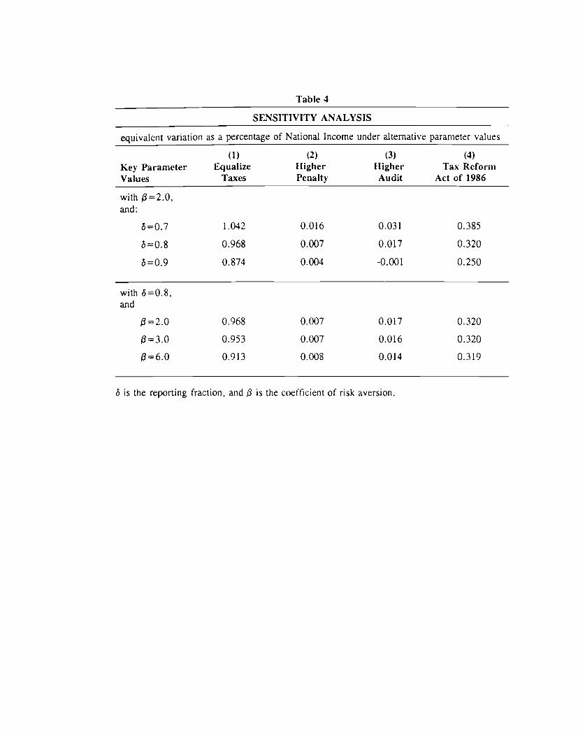
Table 4

SENSITIVITY ANALYSIS

equivalent variation as a percentage of National Income under alternative parameter values

Key ParameterValues

(1)

EqualizeTaxes

(2)HigherPenalty

(3)HigherAudit

(4)Tax Reform

Act of 1986

with 13=2.0,and:

ô=0.7 1.042 0.016 0.031 0.385

ô=0.8 0.968 0.007 0.017 0.320

ô=0.9 0.874 0.004 -0.001 0.250

with 5=0.8,and

13=2.0 0.968 0.007 0.017 0.320

13=3.0 0.953 0.007 0.016 0.320

13=6.0 0.913 0.008 0.014 0.319

ô is the reporting fraction, and 13 is the coefficient of risk aversion.

Tab

le 5

RE

SU

LTS

FR

OM

IN

CR

EA

SE

D E

NF

OR

CE

ME

NT

WIT

H E

IGH

T H

OU

SEH

OL

DS (

fi=

6.O

)

Hig

her P

enal

ty

Hig

her A

udit

Rat

e

Inco

me

Equ

ival

ent

Equ

ival

ent

Cla

sse?

R

epor

ting"

R

eal E

stat

e"

Var

iatio

ns

Rep

ortin

gb

Rea

l Est

ate"

V

aria

tions

0-5K

1.

0037

1.

0049

$-

0.0

2

5-10

K

1.00

39

1.00

41

$- 0

.13

10-2

0K

1.00

39

1.00

24

$ 0.

24

20-3

0K

1.00

39

1.00

15

$ 1.

75

30-5

0K

1.00

40

1.00

08

$ 3.

78

50-l

OO

K

1.00

42

0.99

98

$ 8.

14

100-

200K

1.

0055

0.

9988

$

2.20

200K

+

1.00

62

0.99

94

$-21

.42

Tot

al

1.00

01

0.99

98

$157

.1 m

illio

n

1.03

44

1.03

16

5-

0.19

1.03

42

1.02

56

$-

1.39

1.03

39

1.01

30

5-

1.76

1.03

35

1.00

62

S 3.

82

1.03

29

1.00

10

$ 9.

33

1.03

11

0.99

48

$ 18

.47

1.02

49

0.99

51

$- 4

3.74

1.02

31

0.99

90

$-20

6.59

1.03

33

0.99

96

$41.

5 m

illio

n

a:

Inco

me

clas

ses

and

wel

fare

m

easu

res

are

show

n in

198

3 do

llars

per

hou

seho

ld.

The

tota

l ro

w s

how

s

the

sum

ove

r al

l 79

,862

,000

hou

seho

lds,

in

mill

ions

of

1983

dol

lars

.

b:

The

se n

umbe

rs re

pres

ent

ratio

s of

fina

l eq

uilib

rium

val

ue to

ben

chm

ark

valu

e.