Tax evasion, firm dynamics and growth∗

Emmanuele Bobbio†

Bank of Italy

October 19, 2016

Abstract

Italy’s growth performance has been lacklustre in the last two decades.The economy has low R&D intensity; firms are smaller and less likely togrow or exit than firms in other advanced countries; the shadow economyis large. I show how these features arise simultaneously in a Schum-peterian growth model with heterogeneous firms where the tax auditingprobability increases with firm size. Tax evasion confers a cost advantageover competitors. In equilibrium, small firms invest less in innovationbecause growing entails a (shadow) cost of fiscal regularization. Unfaircompetition forces other firms to lower the mark-up they charge for theirnew products, reducing the incentive to innovate. Market selection ishampered, further lowering the aggregate growth rate along the extensivemargin. I calibrate the model on Italian firm-level data for the period1995-2006 and find that enforcing taxes would have increased the long-run growth rate from 0.9% to 1.1%. The market share of high type firmswould have been 8 percentage points higher and average firm size 25%higher. Also, I find that lowering the tax burden can have a significantimpact on growth when the shadow economy is large, while the effect isnegligible when taxes are enforced.

∗I thank Martino Tasso, Rosaria Vega Pansini, Alfonso Rosolia, Francesca Lotti, MatteoBugamelli, Paolo Sestito, Paolo Finaldi Russo, Silvia Magri and Claudio Michelacci for helpfuldiscussions and comments. All remaining errors are mine. The views set out in this paper donot necessarily reflect those of the Bank of Italy.†emmanuele.bobbio@bancaditalia.it

1 Introduction

Italy has been experiencing a prolonged period of anaemic growth, even priorto onset of the financial crisis. Labor productivity per hour worked in the non-agricultural business sector has increased at an annual rate of 0.9% between1995 and 2006. The Italian business sector is characterized by a low R&D in-tensity and it is populated by a prevalence of small firms displaying a weak“up-or-out” dynamics. R&D expenditure by private companies in Italy wasapproximately 0.5% of GDP (as opposed to 1.3% in France and 1.8% in theU.S.). Regarding firm demographics, businesses with fewer than 50 employeesaccounted for 63.5% of employment between 2001 and 2010 (35.9% and 29.9%);83.4% of entering firms were still in the market after three years (78.7% and71.7%) and only 3.6% of them had grown in size (4.0 and 6.2%) – Criscuolo,Gal, and Menon (2014) and, with specific regard to Italy, Manaresi (2015).In this paper I show how tax evasion may explain these features of Italian firmsalong with a weak aggregate economic performance. I use a model of endoge-nous growth – Romer (1990), Aghion and Howitt (1992) and Grossman andHelpman (1991) – accounting for firm dynamics – Klette and Kortum (2004) –and firm heterogeneity – Lentz and Mortensen (2008) and Acemoglu, Akcigit,Bloom, and Kerr (2013) – and augment it with a game of tax evasion, price,quantity and innovation decisions.Tax evasion in Italy is high, both in absolute terms and by international com-parison. According to estimates in Schneider and Enste (2000) and Schneiderand Williams (2013) the size of the shadow economy in Italy stands at approxi-mately 25% of GDP as opposed to 15% in France and 8% in the U.S.. A similarnumber for Italy is found by Ardizzi, Petraglia, Piacenza, and Turati (2014)using the currency demand approach and detailed cash withdrawal data. Istat(2011) reports an official estimate of around 18% for the period 2000-2008 and12% regarding the share of irregular workers on total employment. More re-cently and with reference to the period 2011-2013, official estimates have beenrevised downward to approximately 13% for the size of the shadow economy asa fraction of GDP and upward to 15% for the share of irregular workers – Istat(2015). Cannari and d’Alessio (2007) use survey data and find evidence thatthe propensity to evade taxes has increased between 1992 and 2004.The crucial assumption underlying the results of the paper is that small firmsare less likely to be monitored by the tax enforcement authority than largefirms, other things equal. According to data published by the Italian Rev-enue Agency (IRA) the fraction of firms with a turnover above 100mln euros(approximately 300 employees) monitored in 2015 was 39%, as opposed to 2%for sole-proprietorship and small firms – Agenzia delle Entrate (2015). Also,sole-proprietorship enterprises concealed approximately 1/3 of their turnover,according to estimates by IRA based on tax audit data for the period 2007-2008 and corrected for possible biases due to the non-random nature of audits –Ministero dell’Economia e delle Finanze (2014). Finally, the Italian economy ischaracterized by a remarkably high self-employment rate, 28.3% between 1995and 2006 according to the OECD, as opposed to 9.5% in France and 7.7% in the

1

U.S.. Torrini (2005) provides evidence that differences in self-employment ratesacross countries are partly explained by differences in tax evasion opportunities.The fundamental source of distortions in the model is that tax evasion confersa cost advantage to firms with a greater scope for evading taxes – an advantagewhich is greater the higher the statutory level of taxes. A small firm that in-novates and grows gives up this cost advantage; thus, she incurs a shadow costof “fiscal regularization”. In addition, the “unfair competition” brought aboutby firms with a greater scope tax evasion forces innovative firms to lower themarkup on their products. Both, the regularization cost and unfair competitionreduce the incentive to innovate for incumbent firms and the aggregate rate oftechnological progress with it. This outcome is reinforced via two general equi-librium channels. The low innovation effort exerted by incumbent firms weakensselection and small, less productive and less innovative firms tend to stay in themarket. In so doing, tax evasion also reduces the aggregate growth rate alongthe extensive margin, because innovative firms account for a smaller share ofresources and economic output in equilibrium. Finally, the higher prevalenceof small firms in equilibrium increases the degree of unfair competition in theeconomy. Such circularity may disrupt the growth process, when the scope fortax evasion varies significantly across differently sized firms and statutory taxrates are high. In this case the benefits from tax evasion may be large enoughthat incumbent firms stop innovating, there is no selection and there are nolarge firms in equilibrium.I calibrate the model using statistics for the aggregate growth rate and for thesize of the shadow economy in Italy over the period 1995-2006 and targeting firmdemographics that I compute from micro-data. I find that enforcing taxes wouldhave raised the growth rate permanently from 0.9 to 1.1%, both by increasingindividual incentives to innovate and by shifting the composition of the econ-omy towards more innovative firms. Entry would have been lower contributingnegatively to growth instead. Also, enforcing taxes would have enhanced firmdynamics: the probability of leaving the market within one year of entry wouldhave been 1 percentage point higher; the employment growth rate of survivingfirms would have increased by 2/3 and mean firm size would have been a quar-ter higher. Enforcing taxes increases the revenue stream for the governmentthat can cut statutory rates. This cut has a negligible effect on growth, whentax evasion has been already eliminated – consistently with mixed findings inthe empirical literature regarding the relationship between taxes and growth.However, I find that when the size of the shadow economy is large instead, cut-ting statutory rates does boost growth, because it reduces the benefits from taxevasion: in the calibrated version of the model reducing the tax burden by 1percentage point by cutting corporate taxes raises the long run growth rate by4 bases points.The paper is related to the recent body of literature that emphasizes the impor-tance of firm heterogeneity and efficient resource allocation for the level of pro-ductivity – Bartelsman, Haltiwanger, and Scarpetta (2012), Hsieh and Klenow(2009), Restuccia and Rogerson (2008) – and its evolution over time – Acemogluet al. (2013), Lentz and Mortensen (2008) – as well as of size related distortions

2

– Guner, Ventura, and Xu (2008), Hopenhayn (2014). The literature has de-veloped towards a more granular exploration of the sources of inefficiencies ineconomies with heterogeneous firms. Particular attention has been devoted tostudying the role of credit frictions for the process of economic development,Buera, Kaboski, and Shin (2011), Midrigan and Xu (2014), Moll (2014). In thecontext of the Klette and Kortum (2004) framework, Aghion, Akcigit, Cage,and Kerr (2016) have considered the relationship between taxation, corruptionand aggregate growth when investment in a public good can improve the inno-vation process, while Akcigit, Alp, and Peters (2016) have analyzed how limitsto delegation can help explaining differences in firm demographics between In-dia and the U.S.. Lentz and Mortensen (2015) study optimal taxation withinthis framework, while Acemoglu et al. (2013) evaluate the impact of innovationpolicies.The paper is organized as follows: in section 2 I outline the model, characterizethe solution to the game determining price, quantity, innovation and tax evasiondecisions and characterize the balance growth path equilibrium of the economy.In section 3 I discuss identification of the model parameters and outline thecalibration strategy. Results are discussed in section 4 and their robustness istested in section 5. Section 6 concludes.

2 The model

I extend the Schumpeterian growth model – Aghion and Howitt (1992), Gross-man and Helpman (1991), Romer (1990) – with heterogeneous firms – Kletteand Kortum (2004), Lentz and Mortensen (2008) – to account for tax evasion.A sketch of the basic framework is as follows: there is a representative house-hold consuming a final good that is competitively produced by combining acontinuum of intermediate products. The productivity of an intermediate prod-uct is the result of past innovations. A firm realizing an innovation prices outthe producer that was supplying the previous vintage of the intermediate goodand charges the final good producer a markup. The firm enters the intermediateproduct market if it was a potential entrant, or grows in size, if it was already anincumbent, adding a market niche to her portfolio of leading-edge technologies.Tax evasion alters competition between producers of different vintages of thesame intermediate good, distorting the markup and changing the perspectivegains from investing in innovation and growing.

2.1 Final good: consumption, production

Time is continuous, the demand side of the economy consists of a representativehousehold supplying labor, L, inelastically and choosing consumption of the

3

final good, C, and asset holdings, H, to maximize utility:

U0(H0) = maxCt,Htt≥0

∫ ∞0

lnCte−ρtdt

s.t.: Ht =wtL− PtCt + rtHt

ρ is time discounting and w,P, r denote prices. Asset holdings consist of anexhaustive portfolio of all ownership titles of firms populating the economy, po-tential and incumbent. The solution to the household problem is characterizedby the Euler equation:

CtCt

= rt − ρ−PtPt

(2)

The market for the final good is perfectly competitive. The production tech-nology is Cobb-Douglas and requires a continuum of intermediate products –indexed on the unit interval:

lnYt =

∫ 1

0

ln(Aitxit)di (3)

xi is the quantity of intermediate good i used into production and Ai denotesits productivity level. Profit maximization and perfect competition imply thatthe demand function for intermediate good i is equal to:

xdit =PtYt

(1 + τva)pit=

1

pit(4)

where pi is the price of the intermediate good and τva is the tax rate on valueadded. The second equality follows from normalizing the price of the finalgood so that aggregate expenditure equals 1 + τva and PY/(1 + τva) = 1 ∀t.Substituting (4) into (3) aggregate output can be written as:

lnYt = lnAt −∫ 1

0

ln(pit)di (5)

with:

lnAt ≡∫ 1

0

ln(Ait)di

2.2 Intermediate goods: pricing, tax evasion, innovation

The productivity of a particular intermediate good i is the result of past in-novations, q1i, q2i, . . ., qIiti, where Iit is the number of successive innovationsrealized in product line i up to time t:

Ait =

Iit∏j=1

qji

4

Innovation is modeled as a Poisson process. The arrival probability is a functionof the amount of resources invested in innovation and the incremental step, q,depends on the innovation capacity of the firm, which is discovered upon entryand is permanent.The final good producer is indifferent between paying the price (1 + τva)p forvintage Iit − 1 of variety i or paying the price (1 + τva)pqIiti for vintage Iit.As argued below and shown formally in appendix A, the payoff function isstrictly increasing in p. Then, in a Stackelberg equilibrium the firm that hasthe know-how to produce the latest vintage, which I assume moves first andI refer to as the leader, prices out the follower and becomes the monopolistproducer in market niche i. The firm then enters the market as the supplierof that single product line if it was a potential entrant; or grows to size n + 1if it was a size n incumbent, n denoting the number of market niches wherethe firm is a technological leader. Production of each variety the firm suppliesis carried out at a different establishment and requires labor only, in one toone proportion. The firm must pay taxes on value added, labor, profits andturnover at rates τva, τl, τpf and τto respectively. Or it can conceal part of theoutput. For simplicity suppose that the establishment has an overground and anunderground part, and that the firm decides the fraction of output located in theunderground part, λ ∈ [0, 1], where it does not pay taxes. The tax enforcementauthority visits the establishment with a certain probability, this probabilitygrowing with the amount of output the firm attempts to conceal and with thesize of the firm: Pr′(λx|n) > 0, Pr′′(λx|n) ≥ 0 and Pr(λx|n + 1) ≥ Pr(λx|n).Innovation is carried out in the overground section of the establishment andrequires labor only.1 In the robustness section I also consider the case whereinnovation requires the final good instead of labor, capturing the idea thatinvestments in goods such as ICT can raise productivity or increase the qualityof the intermediate good. I assume that innovation is arbitrarily costly at aplant that has become a technological lagger. Consider a particular marketniche. Let vS , S ∈ L,F be the expected value of an innovation for the leader(L) and for the follower (F ) and w be the aggregate wage level and assume thatwhen indifferent the final good producer buys the latest vintage. Given thedemand function 4, the leader and the follower choose the price pS , tax evasionλS and the amount of resources to invest in innovation ι(γS |S), or equivalently

1Alternatively I could assume that a fraction λ of the investment in innovation is concealedin the underground part of the establishment. In this case the firm pays more profit taxesbut has a lower labor cost. The analysis is somewhat simplified and results are fundamentallyunaffected.

5

the innovation rate γ, to maximize the payoff function Ω:

Ω(pS , λS , γS |nS , vS , S, qL, p−S , w) =π(pS , x(pS , p−S |qL), λS , γS |nS , S, w)

+ γSvS (6)

x(pL, pF |qL) =

1pL

if pL ≤ pF qL0 o.w.

x(pF , pL|qL) =

1pF

if pF qL < pL

0 o.w.

where π is the profit flow:

π(p, x, λ, γ|n, S,w) =(1− τpf1Πλ,γc >0)Πλ,γc (p, x|S,w)− (1− λ)τtopx

+ λΠnc(p, x|w)− (1 + ν) Pr(λx|n)Υ(p, x, λ, γ|S,w)

and Υ is tax gap, ν is the fine the firm must pay on top of taxes if it is caughtby the tax enforcement authority (in Italy the fine is indeed a proportionalconstant):

Υ(p, x, λ, γ|S,w) =λ(τvapx+ τtopx+ τlwx)

+ τpr

[1Π0,γ

c >0Π0,γc (p, x|S,w)− 1Πλ,γc >0Πλ,γ

c (p, x|S,w)]

and Πλ,γc (p, x|S,w) and Πnc(p, x|w) are the profit flows generated in the over-

ground (gross of turnover taxes) and in underground part of the establishmentrespectively - c and nc standing for “compliant” and “not compliant”:

Πλ,γc (p, x|S,w) =(1− λ)Πc(p, x|w)− ι(γ|S,w)

Πc(p, x|w) =px− xςc(w)

Πnc(p, x|w) =(1 + τva)px− xςnc(w)

ςc and ςnc are the constant marginal costs in the overground and undergroundpart of the establishment and are equal to (1 + τl)w and w respectively.

Proposition 1. The subgame perfect Nash equilibrium of the Stackelberg gamewhere the leader and the follower have payoff functions as specified in (6) andwhere the tecnological leader moves first is characterized as follows:

i The firm never picks a price-tax evasion combination (pS , λS) such thatPr(λx(pS , p−S |qL)|nS) = 1;

ii The payoff functions of the leader Ω(·|L) and of the follower Ω(·|F ) arestrictly increasing in the price, provided that pL ≤ pF qL and pF qL < pL,respectively, and that the pairs (pS , λS), S ∈ L,F are sensible, in thesense specified in part i;

iii The follower chooses γF = 0 and pF = pL/qL and λL ∈ [0, 1];

6

iv The leader charges the limit price pL : maxλπ(pL/qL, qLx(pL, pL/qL|qL),λ, 0|nF , F, w) = 0 and picks (λ, γ) to maximize the payoff π(pL, x(pL, pF |qL), λL, γL|nF , F, w) + γLvL.

Proof. See appendix A

A sketch of the proof follows. If the firm were to choose (λ, p) such thatPr(λx(pS , p−S |qL)|nS) = 1 then the expected cost of tax evasion would behigher than paying taxes outright and (0, p) must yield a higher payoff. Asfor part ii, the result hinges on the assumption that the production functionin the final good sector is Cobb-Douglas so that revenues do not depend onthe price the firm charges, while production costs increase in x or, equivalently,decrease in p (see eq. 4) as far as p is lower than the price per efficiency unitcharged by the competitor. In addition, I assume that the probability that thefirm is monitored and caught by the tax enforcement authority decreases thelower amount of output it conceals. This assumption is made so that the taxevasion choice always depends on the price and viceversa – see cases A and C inappendix A – and not only in marginal cases – case B. Since the payoff functionincreases with the price, the leader charges the maximal price such that, evenif the follower tries to exploit the tax evasion margin, it cannot undercut theleader and still make a positive profits. Since I assume that the follower costof innovation is arbitrarily large, there is no reason for it to stay in the marketwhile earning a negative profit flow, therefore it quits market niche i. Theprice level the leader charges depends on his innovation ability captured by qL,which allows the leader to charge a markup to the final good producer, and isconstrained by the operating cost of the follower which the follower can reduceby evading taxes. Finally given the price pL the leader picks the combinationof tax evasion rate λL and innovation effort γL that maximizes profits.

2.3 Intermediate goods: values

There are two types of firm differing in terms of their innovative capacity, z =∈b, g with qg = q > qb = 1. Type b firms (“bad”) are imitators, they areunable to generate improvements that actually enhance the productivity of anintermediate product, while type g firms (“good”) are innovators. There is amass m of potential entrants having access to the same innovation technologyas incumbents, ι(γ). The type of a firm is realized upon entry and it is equalto g with probability φ and to b with probability 1− φ. Also, it is permanent.An incumbent firm adds to her technology portfolio by investing in innovation.Innovation is undirected and whenever a firm realizes an innovation in somemarket niche, some other firm is displaced from that market niche.2 Therefore,

2In facts, in the model some market niches offer a higher expected value than others.Specifically, it would be more profitable for a firm to target market niches where the leaderis more intensely monitored by the tax enforcement authority. I prevent firms from doingso by assumption. The assumption can be justified to a certain extent by appealing to theuncertainty intrinsic to research effort. Also, note that relaxing it would strengthen theargument: large, more productive and more innovative firms would be targeted and be more

7

all firms are subject to the same instantaneous probability of loosing a marketniche and become an n− 1 size firm. I denote such common destruction rate δ.A firm that has one market niche and looses it exits the market.As mentioned above the auditing probability increases with the size of the firm.In particular, I assume that a firm is more intensely scrutinized if it operatesmore than one plant, Pr(λ/p|1) < Pr(λ/p|n) = Pr(λ/p|n+1), ∀λ/p > 0 and n >1 and that once a firm is subject to a high monitoring probability she remainsso, even if her size subsequently drops below 2. I refer to a firm whose size is(or has been) equal to or greater than n = 2 as “large” and to other firms as“small” and use the letters l and s to indicate the degree of scrutiny a firm issubject to.The value of a firm is the sum of the values of the establishments it operates, orequivalently of the market niches where she is a leader.3 Let vfzd be the valueof an establishment operated by a type z ∈ b, g firm having size d ∈ s, land competing against a size f ∈ s, l firm. If the firm is large, the discountedexpected stream of net profits generated by an establishment is equal to:

rvfzlt − vfzlt = max

λ,γ

⟨πfzlt(λ, γ) + γvzlt − δvfzlt

⟩vzlt ≡ζstvszlt + ζltv

lzlt

where ζf is the fraction of product market niches in the economy where the

leader has size equal to f and πfzlt(λ, γ) is short for πt(pL, 1/pL, λ, γ|l, z, w),given that the limit price pL is known from the solution to the Stackelberg gameillustrated above – up to the equilibrium wage level, w. Profits are discountedat the nominal interest rate r; the flow value of the establishment net of capitalgains due to the flowing of time equals net profits, plus the expected capitalgains from expending into a new market niche, minus the expected capitallosses from loosing the technological leadership in the market niche currentlydominated by the firm. Since vszlt < vlzlt, then vzlt < vlzlt. Thus, the stronger

likely to be pushed out of the market than small, less productive, less innovative firms, thusincreasing the shadow cost of regularization, decreasing selection and unfair competition alongthe extensive margin.

3I assume that each establishment pays taxes separately, that innovation is carried out atthe establishment level and that innovation costs cannot be shifted from one establishment toanother. A firm making negative profits at an establishment and positive profits at anotherestablishment would have an incentive to shift innovation costs at the establishment yieldingpositive profits so as to decrease the overall corporate tax bill. These are cases that turnsout to be irrelevant for the empirical application implemented below. Also, in the empiricalapplication a firm with two or more product market niches exerts the same innovation effortat all establishments, regardless of follower characteristics. Therefore I could simply assumeparameter values such that the equilibrium has these features and prove that the value functionis modular across market niches, as in Klette and Kortum (2004) and Lentz and Mortensen(2008), rather than working at the establishment level and aggregating establishments up tothe firm level. Another approach delivering the same result is to assume that profit taxes arecalculated on profits gross of innovation costs, braking the direct dependence of γ on p andλ. In this case the result regarding the effect of tax evasion on aggregate growth would befundamentally unaffected, though the counterfactual implications of changing corporate taxesmight differ, as it should be clear from the analysis in appendix B for the case with no taxevasion.

8

the cost advantage for the follower due to tax evasion (vlzlt− vszlt) and the morewidespread tax evasion (ζs), the lower incentives to invest in innovation for largefirms. I refer to the quantity vlzlt − vzlt as the “extent of unfair competition”.If the firm is small and makes an innovation it grows into a 2 product lines firm,becoming large and subject to a higher degree of scrutiny by the tax enforcementauthority. As a result, while the firm acquires a new market niche, she also mustregularize part of her business at the plant she was already operating, whichentails a shadow cost:

rvfzst − vfzst = max

λ,γ

⟨πfzst(λ, γ) + γ[vzl − (vfzst − v

fzlt)]− δv

fzst

⟩where vfzlt − v

fzst > 0 follows from comparing this expression with that for a

large firm and from the fact that, since a small firm is subject to lower scrutiny,it can implement the same strategy as a large firm, i.e. pick (λfzlt, γ

fzlt, ), and

still make higher profits than a large firm. I refer to the difference vfzlt − vfzst

as the “regularization cost”. Comparing the value function for a small and fora large firm one notices that the regularization cost reduces the expected valueof an innovation. Thus, tax evasion reduces the incentives for small firms toinnovate and grow in size.A type b firm, i.e. a firm such that qb = 1, makes positive profits only if sheis up against a follower that is subject to stricter fiscal enforcement. If thisfirm innovates and grows she looses this cost advantage. Thus, she pays theregularization cost and does not rip any benefit from entering a second marketniche, where she will earn zero profits at most, i.e. πfblt(λ

fblt, γ

fblt) ≤ 0. Therefore

a type b firm will always choose not to invest in innovation, γfbdt = 0, and toremain small. It follows that in equilibrium all large firms must be type g.Finally, as it is clear from the labor market clearing condition outlined below,on a balanced growth path the aggregate wage level, wt, is constant, thus thevalue of a market niche is constant as well. All this considered I can rewrite thesystem of value functions more compactly:

vfb =πfbρ+ δ

, ∀f ∈ s, l (12a)

vfgs = maxλ,γ

⟨πfgs(λ, γ) + γ[vl − (vfgs − v

fgl)]

ρ+ δ

⟩, ∀f ∈ s, l (12b)

vfgl = maxλ,γ

⟨πfgl(λ, γ) + γvl

ρ+ δ

⟩, ∀f ∈ s, l (12c)

where I renamed vl = vgl since only type g firm can be large and I have usedthe Euler equation from the household problem (2) which along with the nor-malization PtYt = 1 + τva implies r = ρ.

9

2.4 General equilibrium

As mentioned above, there is a fix mass of potential entrants, m; firms in theentry pool have access to the same innovation technology as incumbents, ι(γ).Upon realizing an innovation the firm observes her type, g with probability φand b with probability 1−φ, and enters the market with one product line, n = 1.A firm in the entry pool exerts innovation effort γ0 such that the marginal costequals the expected value of entering the intermediate product market and theaggregate entry flow is η = mγ0:

η = mγ0 = mι′−1

φ ∑f∈s,l

ζfvfgs + (1− φ)

∑f∈s,l

ζfvfb

∣∣∣w (13)

The aggregate destruction rate is the result of the innovation activity carriedout by all firms in the economy, new entrants and incumbents, small or large:

δ = η +∑

d∈s,l

∑f∈s,l

γfgdζfgd (14)

The steady state flow equations determining the share of types and leader andfollower sizes across product lines are:

ζfb , f ∈ s, l : η(1− φ)ζf =δζfb (15a)

ζfgs, f ∈ s, l : ηφζf =(γfgs + δ)ζfgs (15b)

ζfgl, f ∈ s, l : (δ − η)ζf + γfgsζfgs =δζfgl (15c)

In steady state the inflow equals the outflow: the inflow of product lines suppliedby type b firms and competing against a follower with size f equals the entryflow η times the probability that the entering firm turns out to be type b, 1−φ,times the probability that the firm ends up competing against a size f follower,which is equal to ζf , since innovation is undirected. With regard to ζfgs, theoutflow is augmented with the probability that an innovation is realized andthe firm becomes large, γfgs. Finally, with regard to large firms, all innovationthat is not realized by new entrants results in the creation of establishmentsowned by large firms, accruing to the stock ζfgl. In addition plants which wereoperated by small, type g firms become part of a large firm further contributingto ζfgl.The mass of intermediate products supplied by small type firms is equal toζs = ζsb + ζlb + ζsgs + ζlgs. Using eqs. (15a) and (15b) and ζl = 1 − ζs – whichfollows from the fact that the measure of product lines is normalized to 1 –I can express ζs as a function of rates characterizing the birth-death processη, δ, γsgs, γlgs and then solve the system of equations (15) recursively:

ζs =η

δ

(γlgs + δ)(γsgs + δ)− φγlgs(γsgs + δ)

(γlgs + δ)(γsgs + δ) + φη(γsgs − γlgs)

10

The wage rate must clear the labor market. Labor supply is exogenous andequal to L. Labor demand is the sum of labor hired for production and forinnovation. One unit of labor produces one unit of output and demand for anintermediate good equals the inverse of the price, eq. (4). The price that a firmcharges for an intermediate product is equal to the type specific innovation step– qz, z ∈ b, g – times the limit price that lowers the follower profits to zero –see proposition 1. This price depends on the ability of the follower to concealproduction, i.e. on its size – f ∈ s, l – and on the cost of production, w (seeappendix A). Labor is also used for innovation both by potential entrants andincumbents, a firm requiring ι(γ)/w units of labor at a plant for that plant togenerate an innovation at rate γ. Thus, the equilibrium wage rate solves:

L = mι(ηm |w

)w

+∑

d∈s,l

∑f∈s,l

ζfdι(γfgd|w)

w+

∑z∈b,g

∑f∈s,l

ζfz1

pfz(16)

Finally, from eq. (5) the aggregate growth rate is equal to:

A

A=

ηφ+∑

d∈s,l

∑f∈s,l

γfgdζfgd

ln q (17)

Definition 1. Given the normalization PtYt = 1+τva, a Balanced Growth PathEquilibrium consists of:

• an aggregate state w, r, Pt, Att≥0, ζ characterized by a constant wagew, a constant interest rate r, a final good price sequence Ptt≥0, a TFPsequence Att≥0 and a constant vector of market niche shares ζ = ζsb , ζlb,ζsgs, ζ

lgs, ζ

sgl, ζ

lgl

• individual consumption Ctt≥0 and production decisions Ytt≥0 by thehousehold and by the final good producer respectively, as well as constantdecisions by intermediate good producers for prices p = psb, plb, psgs, plgs,psgl, p

lgl quantities x = xsb, xlb, xsgs, xlgs, xsgl, xlgl tax evasion rates λ =

λsb, λlb, λsgs, λlgs, λsgl, λlgl and innovation rates γ = γsb , γlb, γsgs, γlgs, γsgl, γlgland associated values v = vsb , vlb, vsgs, vlgs, vsgl, vlgl

such that:

i. given Ptt≥0, factor demand in the final good sector is optimal, i.e.Ytt≥0,p,x satisfy eq. (4);

ii. given w and v, individual choices for p,x,λ,γ sustain the the subgameperfect Nash equilibrium of the Stackelberg game, i.e. they satisfy theconditions in Proposition 1.iv;

iii. given w, r, δ,p,x,λ,γ, individual values v satisfy the value functionseq. (12);

11

iv. given w, ζ,v the innovation effort exerted by potential entrants is opti-mal, i.e. η satisfies eq. (13);

v. given the vector of market niche shares ζ, the entry rate η and incumbentinnovation rates γ yield the destruction rate δ, i.e. eq. (14) holds;

vi. given the birth-death process as characterized by the tuple η, δ,γ, thevector of market niche shares ζ satisfies the system of stock-flow equations,eq. (15);

vii. the wage w clears the labor market, i.e. w,x, η,γ satisfy eq. (16);

viii. the market for the final good clears Ct = Yt and, under the chosen nor-malization, Pt = (1 + τva)/Yt, ∀t ≥ 0;

ix. r, Pt, Ctt≥0 satisfy the Euler equation eq. (2), i.e. r = ρ;

x. Yt, Att≥0,p satisfy eq. (5), Ytt≥0 and 1/Ptt≥0 grow at the samerate as technology Att≥0 which evolves as in eq. (17).

2.5 Firm size distribution

Let mgl[n] be the mass of good type, large firms supplying n product lines.By equating the inflow and outflow I obtain the following system of differenceequations:

n > 2 : mgl[n]n(δ + γl) =mgl[n+ 1](n+ 1)δ +mgl[n− 1](n− 1)γl

n = 2 : mgl[2]2(δ + γl) =mgl[3]3δ +mgl[1]1γl + γsgsζsgs + γlgsζ

lgs

n = 1 : mgl[1]1(δ + γl) =mgl[2]2δ

where γl ≡∑f∈s,l ζ

fglγ

fgl/∑f∈s,l ζ

fgl is the innovation rate chosen by large

firms across product lines, on average. By inspection it can be verified thatmgl[n] = aθn−2

l /n solves the first equation with θl ≡ γl/δ and a equal to someconstant. Next I use the first and third expressions to write mgl[3] and mgl[1]in terms of mgl[2], substitute out for mgl[3] and mgl[1] in the second expression,solve for a and obtain the closed form solution:

mgl[n] =

θs(1+θl)θ

n−2l

n , n ≥ 2

θs, n = 1(18)

θs ≡ζsgsγsgsδ

+ ζlgsγlgsδ

θl ≡γlδ

12

The overall firm size distribution µ[n] is then equal to:

µ[n] =

θs(1+θl)

Θ

θn−2l

n , n ≥ 2θηΘ , n = 1

(19)

Θ ≡ θη + θs(1 + θl)ln 1

1−θl − θlθ2l

where Θ is the total mass of firms in the economy, θη ≡ η/δ and I made useof θη = ζs + θs which follows from adding eq. (15a) to eq. (15b) and dividingthrough by δ.4 The firm size distribution is entirely determined by three quan-tities: θη ≡ η/δ, θs ≡ ζsgsγsgs/δ + ζlgsγ

lgs/δ and θl ≡ γl/δ. Such quantities reflect

the tension between the sullying effect of entry, θη, and the cleansing effect ofthe innovation effort exerted by incumbents, whether small or large, θs and θl.The intensity of the creative destruction process, δ, is irrelevant for the steadystate degree of selection in the economy; what matters is instead how δ brakesdown into η on one hand and γsgs, γ

lgs, γl on the other. Tax evasion lowers θs

relative to θη – both due to the regularization cost and to unfair competition –compressing the size distribution to the left. Furthermore it reduces θl relativeto θη because of unfair competition.

3 Identification and calibration strategy

I assume that the monitoring probability function and innovation cost functionhave the power form:

Pr (λx, n) = an(λx)a (20)

an =

as if n = 1

al if n > 1

with as ≤ al and a ≥ 1, and:

ι(γ|w) = (1 + τl)wι0γ1+ι1 (21)

with ι0 > 0 and ι1 > 0.In appendix B I characterize the model solution in the case with no tax evasionas → ∞ and show that under the assumption that ι is a power function and

4The total mass of firms is computed noting that:

∞∑n=2

θn−2l

n=

1

θ2l

[−θl +

∞∑n=1

θnln

]=

1

θ2l

[−θl +

∞∑n=1

∫ θl

0xn−1dx

]

=1

θ2l

[−θl +

∫ θl

0

∞∑n=1

xn−1dx

]=

1

θ2l

[ln

1

1− θl− θl

]

13

given that the risk free rate r is known, the model is identified only up to oneof the three parameters m, ι0, ι1, if no information on innovation spending isavailable:

Proposition 2. Assume that ι(·) is as in (21) and that there is no tax evasion(i.e. as →∞, if Pr is as in eq. 20) then:

i. there is one and only one balance growth path as defined in Definition 1;

ii. if the risk free rate can be observed, then the model is identified only up toone of the three parameters m, ι0, ι1, if no data on innovation spendingis available.

Proof. (i.) See appendix B. (ii.) In appendix B I show that the equilibriumconditions can be rewritten as η = ξ0(m,φ, ι1)γ, δ = ξ1(φ, ξ0)γ, ζg = ξ2(φ, ξ0, ξ1)and γ = ξ3(ιw0 , ι1, q, ξ1), where ιw0 ≡ wι0, and that the aggregate growth rate is(ξ0+ξ2)γ ln q. Then, given φ, ξ0, q, firm demographics, their evolution and theaggregate growth rate are fully determined. This provides four condition for fiveunknowns leaving one of the three parameters m, ιw0 , ι1 undetermined. Then,for example, given knowledge of ι1 I can invert ξ0 and ξ3 (which are invertible)and recover m and ιw0 respectively. As for L, note that any w can be rationalizedby picking the appropriate level of L and w determines the number of labor unitsused in the innovation process, given a value for ι(·), or equivalently γ. Thus wis one-to-one with the relative size of a type g vs. a type b firm.

Instead, with tax evasion and different degrees of tax enforcement acrossfirms (i.e. as finite, as < al and ζl > 0) the model is fully identified, becauseat least two (and up to four) realizations of the innovation intensity choice areobserved, for example γlgs = ι′−1(·|ι0, ι1) and γlgl = ι′−1(·|ι0, ι1) 5. Then ι1 canbe identified in theory by comparing the growth rate of small and large firms,for instance. In practice, small firms tend to be younger and younger firms tendto grow faster, possibly for reasons other than innovation. A possibility thatI do not explore here is to compare the growth rate of small and large firmsconditional on age. Instead I tune this parameter based on values found in theliterature, as discussed below, and evaluate the robustness of counterfactuals tochanges in ι1.In appendix B I provide a formal argument and describe a practical strategyfor calibrating the model without tax evasion, given ι1. The target statisticsare reported in table 1. In short, to the extent that incumbent firms invest ininnovation, the exit probability declines with age; the entry rate and a point onthe hazard curve provide information on η and δ – or, analogously, two pointson the hazard curve, since in steady state the entry rate equals the exit rate anda particular hazard function maps only into one exit rate. The relationship be-tween average firm size and age is indicative of the magnitude of γ, given δ andφ – these three quantities fully describing the evolution of an incumbent firm interms of the number of market niches. Finally, any aggregate growth rate can

5In the case of potential entrants one only observes mγ0 and not γ0 directly.

14

always be rationalized by picking an appropriate level for q – see eq. (17). Asfor the model with tax evasion, I set a = 1 in (20) and then pick as and al toreplicate the incidence of tax evasion in the economy.Regarding ι1, Acemoglu et al. (2013) estimate a model similar to Lentz andMortensen (2008) on a sample of innovative firms using R&D and patent dataand find ι1 = 1.75. They also discuss various micro-econometric estimateswhich are obtained either by examining the relationship between R&D expen-diture and patents or the response of R&D expenditure to changes in taxes andsubsidies. The empirical results in these studies point to a value for ι1 in therange [0.7, 2.3]. Instead Lentz and Mortensen (2008) structurally estimate theirmodel with three types on a panel of Danish firms with at least 20 employeesusing data on wages and value added and find ι1 = 3.73. I set ι1 = 2 and thenin the robustness section consider how results are affected by changing the valueof this parameter.I compute firm demographics using social security data covering the universe ofItalian employer businesses between 1990 and 2013. The data contains informa-tion on the number of employees and the wagebill, sector and province, alongwith entry and exit dates.6 I aggregate observations at the firm level, using thefiscal code as the definition for what constitutes a firm. I restrict attention tothe non-agricultural business sector (NACE R1.1 sector C to K) and focus onthe years between 1995 and 2006, i.e. after the recovery that followed the 1992recession and before the onset of the financial crisis. Descriptive statistics arereported in table 5 of appendix C.I consider the 5 cohorts born between 1995 and 1999 and follow them throughto 2006. The left panel of figure 3 displays the exit probability derived from lifetable estimates of the survival functions for each of the 5 cohorts along with thegrowth rate of average size by age – right panel. I average across cohorts andtake as targets for the calibration the average hazard between age 6 and 8 andbetween age 9 and 11 and the average growth rate between age 9 and 11. Thereason for disregarding earlier years is that other mechanisms, such as learningor time-to-build, might be more important in explaining the exit rate or firmgrowth in the first few years of a firm life-cycle – Jovanovic (1982) and Ericsonand Pakes (1995). Indeed, average firm size doubles within one year of entering(not reported).Regarding the level of tax evasion, I assume that large firms do not evade taxes(al →∞) and target the fraction of underground full time equivalent employeesestimated by the National Statistical Institute for the period under considera-tion in Italy – Istat (2011). The assumption that large firms do not evade isa simplification which is dictated by the lack of empirical evidence regardingthe propensity to evade taxes across different size classes. In facts, the Ital-

6The data covers all legal entities making social security contributions for at least oneemployee worker during at least a month in a given year. Entry (Exit) dates are defined asthe earliest entry (latest exit) date of the legal entities sharing the same fiscal code. Withregard to exit I limit the attention to exits which are flagged in the same year when the exitis supposed to occur. See Adamopoulou, Bobbio, De Philippis, and Giorgi (2016a) for a morethorough description of the data.

15

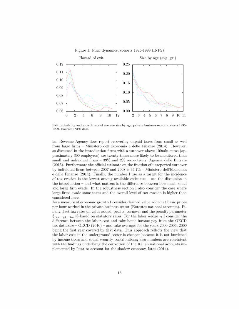
Figure 1: Firm dynamics, cohorts 1995-1999 (INPS)

0.06

0.07

0.08

0.09

0.10

0.11

0.12

0 2 4 6 8 10 12

Hazard of exit

0.00

0.05

0.10

0.15

0.20

0.25

2 3 4 5 6 7 8 9 10 11

Size by age (avg. gr.)

Exit probability and growth rate of average size by age, private business sector, cohorts 1995-1999. Source: INPS data

ian Revenue Agency does report recovering unpaid taxes from small as wellfrom large firms – Ministero dell’Economia e delle Finanze (2014). However,as discussed in the introduction firms with a turnover above 100mln euros (ap-proximately 300 employees) are twenty times more likely to be monitored thansmall and individual firms – 39% and 2% respectively, Agenzia delle Entrate(2015). Furthermore the official estimate on the fraction of unreported turnoverby individual firms between 2007 and 2008 is 34.7% – Ministero dell’Economiae delle Finanze (2014). Finally, the number I use as a target for the incidenceof tax evasion is the lowest among available estimates – see the discussion inthe introduction – and what matters is the difference between how much smalland large firm evade. In the robustness section I also consider the case wherelarge firms evade same taxes and the overall level of tax evasion is higher thanconsidered here.As a measure of economic growth I consider chained value added at basic pricesper hour worked in the private business sector (Eurostat national accounts). Fi-nally, I set tax rates on value added, profits, turnover and the penalty parameterτva, τpf , τto, ν based on statutory rates. For the labor wedge τl I consider thedifference between the labor cost and take home income pay from the OECDtax database – OECD (2016) – and take averages for the years 2000-2006, 2000being the first year covered by that data. This approach reflects the view thatthe labor cost in the underground sector is cheaper because it is not burdenedby income taxes and social security contributions; also numbers are consistentwith the findings underlying the correction of the Italian national accounts im-plemented by Istat to account for the shadow economy, Istat (2014).

16

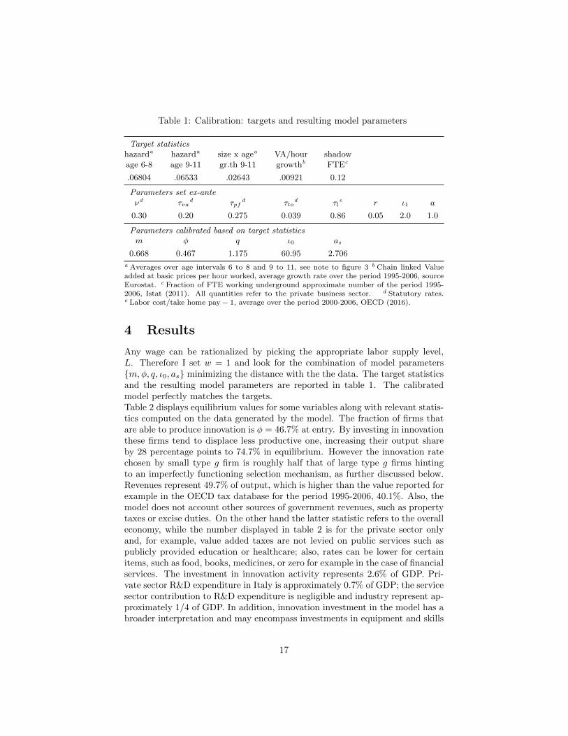
Table 1: Calibration: targets and resulting model parameters

Target statisticshazarda hazarda size x agea VA/hour shadow

age 6-8 age 9-11 gr.th 9-11 growthb FTEc

.06804 .06533 .02643 .00921 0.12

Parameters set ex-ante

νd τvad τpf

d τtod τl

e r ι1 a

0.30 0.20 0.275 0.039 0.86 0.05 2.0 1.0

Parameters calibrated based on target statisticsm φ q ι0 as

0.668 0.467 1.175 60.95 2.706

a Averages over age intervals 6 to 8 and 9 to 11, see note to figure 3 b Chain linked Valueadded at basic prices per hour worked, average growth rate over the period 1995-2006, sourceEurostat. c Fraction of FTE working underground approximate number of the period 1995-2006, Istat (2011). All quantities refer to the private business sector. d Statutory rates.e Labor cost/take home pay− 1, average over the period 2000-2006, OECD (2016).

4 Results

Any wage can be rationalized by picking the appropriate labor supply level,L. Therefore I set w = 1 and look for the combination of model parametersm,φ, q, ι0, as minimizing the distance with the the data. The target statisticsand the resulting model parameters are reported in table 1. The calibratedmodel perfectly matches the targets.Table 2 displays equilibrium values for some variables along with relevant statis-tics computed on the data generated by the model. The fraction of firms thatare able to produce innovation is φ = 46.7% at entry. By investing in innovationthese firms tend to displace less productive one, increasing their output shareby 28 percentage points to 74.7% in equilibrium. However the innovation ratechosen by small type g firm is roughly half that of large type g firms hintingto an imperfectly functioning selection mechanism, as further discussed below.Revenues represent 49.7% of output, which is higher than the value reported forexample in the OECD tax database for the period 1995-2006, 40.1%. Also, themodel does not account other sources of government revenues, such as propertytaxes or excise duties. On the other hand the latter statistic refers to the overalleconomy, while the number displayed in table 2 is for the private sector onlyand, for example, value added taxes are not levied on public services such aspublicly provided education or healthcare; also, rates can be lower for certainitems, such as food, books, medicines, or zero for example in the case of financialservices. The investment in innovation activity represents 2.6% of GDP. Pri-vate sector R&D expenditure in Italy is approximately 0.7% of GDP; the servicesector contribution to R&D expenditure is negligible and industry represent ap-proximately 1/4 of GDP. In addition, innovation investment in the model has abroader interpretation and may encompass investments in equipment and skills

17

improving the productivity of the firm, both in terms of production efficiencyor product quality. All in all, I interpret the model outcome of a 2.6% innova-tion investment share of GDP as a reasonable number, perhaps on the low side.As shown below, reducing the value of ι1 – towards the quadratic case as inAcemoglu et al. (2013) – increases this figure along with the estimated cost oftax evasion, in terms of a lower long-run aggregate growth rate. The entry rate(or equivalently the exit rate) is 5.8% accounting for 2/3 of the correspondingfigure reported in official statistics, approximately 8.5%. As remarked abovethe calibration aims at capturing the component of firm dynamics fueled by in-novation and it abstracts from other mechanisms such as imperfect informationwhich are likely to play an important role especially in the first few years of afirm life-cycle, or from supply and demand shocks. 10.6% of firms that are bornduring a given year t exits by the end of year t + 1. Average employment size– including underground employment – of surviving businesses grows by 1.6%a year between age 9 and 11.7 Average firm size in the economy in terms ofproduct lines, or equivalently turnover or value added, is 1.62.

4.1 Policy experiment: enforcing taxes

I now consider the effect of curbing tax evasion. Results are reported in thesecond row of table 2. As as grows to infinity tax evasion decreases. In the limitthe long run growth rate increases by 0.2 percentage points from 0.92 to 1.13%.Such a change comes about through several channels. As vfgs → vfgl in eq. (12b)the cost of regularization disappears and small innovative firms increase theirinnovation effort to the level of that of large firms, γgs → γgl. Because unfaircompetition also fades, vsgd → vlgd in eqs. (12b) and (12c), both small and largeinnovative firms increase their innovation expenditure further. The aggregatedestruction rate (δ) increases despite the weakening entry flow (η) which is dueto the decline in the value of being a small firm, when the scope for tax eva-sion vanishes – all firms are small when they enter the market. The increasedinnovation expenditure by innovative firms and the drop in the entry rate bothcontribute to stricter selection. Small, less productive firms are pushed out ofthe market and the share of value added produced by innovative firms increasesfrom 74.7 to 82.4%. Thus, the aggregate growth rate increases both along theintensive and along the extensive margin. The negative contribution from thedecline of entry is mitigated by the fact that only a fraction φ = 0.47 of entriesis associated with an improvement in productivity, eq. (17). Finally, note thatthe general equilibrium effect via the labor market is also positive. Since moreproductive firms require less labor for production, the compositional shift to-wards more productive firms frees up resources, the wage declines lowering thecost of innovation and part of the labor is reabsorbed into innovative activitieswhose share rises from 3.0 to 4.1% of employment (not reported).As for firm demographics, a higher degree of tax enforcement is also associated

7This is the growth rate of actual size in terms of the total number of employees, includingthose underground, as apposed to the figure reported in table 1 which refers to employees forwhich the firm pays social security contributions.

18

Tab

le2:

Mai

nre

sult

s:ca

lib

rate

dm

od

elan

dco

unte

rfact

uals

λs

γgl

γgs

ηδ

ζ gτ pf

τ va

τ to

τ lw

gr.

thre

v.

inn.

shad.

ent.

ex.1

ygr.

9-1

1E

(sz.

)

Calibr.

28.4

0.0

593

0.0

327

0.0

364

0.0

765

0.7

47

27.5

20.0

3.9

86.0

1.0

00.9

249.7

2.6

11.6

5.8

10.6

1.6

1.6

2

Low

erev

asi

on

as

=∞

0.0

0.0

694

0.0

694

0.0

282

0.0

854

0.8

24

27.5

20.0

3.9

86.0

0.9

61.1

355.1

3.5

0.0

5.6

11.6

2.6

2.0

3E

v./

217.2

0.0

636

0.0

516

0.0

335

0.0

818

0.7

82

27.5

20.0

3.9

86.0

0.9

81.0

352.5

2.9

5.8

5.8

11.2

2.1

1.7

7

No

evasi

on

(as

=∞

)ta

xes

↓τ pf↓

0.0

0.0

684

0.0

684

0.0

326

0.0

874

0.8

01

0.0

20.0

3.9

86.0

0.9

81.1

352.5

3.6

0.0

6.0

11.9

2.5

1.8

6τ va↓

0.0

0.0

694

0.0

694

0.0

282

0.0

854

0.8

24

27.5

7.0

3.9

86.0

0.9

61.1

349.7

3.5

0.0

5.6

11.6

2.6

2.0

3τ to↓

0.0

0.0

694

0.0

694

0.0

282

0.0

854

0.8

24

27.5

20.0

0.0

86.0

1.0

21.1

352.6

3.7

0.0

5.6

11.6

2.6

2.0

3τ l

↓0.0

0.0

694

0.0

694

0.0

282

0.0

854

0.8

24

27.5

20.0

3.9

62.3

1.1

01.1

349.7

3.5

0.0

5.6

11.6

2.6

2.0

3τ↓

0.0

0.0

694

0.0

694

0.0

282

0.0

854

0.8

24

27.5

20.0

3.9

62.3

1.1

01.1

349.7

3.5

0.0

5.6

11.6

2.6

2.0

3

Low

erta

xes

(as

as

inb

ench

mark

)

τ pf↓

28.3

0.0

597

0.0

411

0.0

376

0.0

796

0.7

48

12.5

20.0

3.9

86.0

1.0

10.9

648.7

2.8

11.3

5.9

11.0

1.8

1.6

1τ va↓

28.3

0.0

599

0.0

361

0.0

360

0.0

776

0.7

53

27.5

16.6

3.9

86.0

1.0

00.9

448.7

2.6

11.2

5.8

10.8

1.7

1.6

4τ to↓

28.3

0.0

607

0.0

376

0.0

361

0.0

786

0.7

55

27.5

20.0

1.8

86.0

1.0

20.9

648.7

2.8

11.1

5.9

10.9

1.8

1.6

5τ l

↓28.4

0.0

596

0.0

342

0.0

362

0.0

771

0.7

50

27.5

20.0

3.9

80.4

1.0

30.9

348.7

2.6

11.4

5.8

10.7

1.7

1.6

3

19

with a higher early exit probability (the probability for a firm born in t of notsurviving to the end of t+1 increases by 1 percentage point) and with a markedincrease in the rate of firm expansion (average firm size rises with each year ofage by 2.6 as opposed to 1.6%, between age 9 and 11). As a result mean firmsize increases by 24.8%.The third row displays results for the case where as is increased so to halve thefraction of underground employment in the economy. In this case the growthrate increases by 0.1 percentage point to 1.03. With a higher level of tax enforce-ment, the fraction of market niches supplied by large firms grows from 59.1% to66.5% (not reported). Thus not only selection contributes to growth by increas-ing the share of economic activity commanded by firms engaging in innovation,but it also decreases the scope for unfair competition, further sustaining in-novative activity and long-run growth, vl ≡ ζsv

sgl + (1 − ζs)v

lgl in eqs. (12b)

and (12c).

4.2 Policy experiment: lowering taxes

With no tax evasion the proceeds collected by the government increase by 5.4percentage points. In the row from 5 to 9 of table 2 I report results for the casewhere such resources are used to lower taxes. The effect on aggregate growth isnil. In facts, the analysis in appendix B indicates that value added taxes andthe labor wedge have no effect on aggregate growth, while a cut in corporate orturnover taxes have an ambiguous effect, when labor is the only input enteringthe innovation process and there is no tax evasion.Results are different when there is tax evasion. As displayed in the bottom partof table 2, a cut in statutory tax rates such to reduce government revenues by1 percentage point has a significant impact on the long run rate of economicexpansion which increases by approximately 4 basis points in the case of a cut incorporate and turnover taxes. This is essentially because cutting taxes reducesthe benefits from tax evasion and thus both, the cost of regularization and theextent of unfair competition, in a similar manner as enforcing taxes.

5 Robustness

5.1 Innovation via the final good

Suppose innovation requires investing into the final good instead of labor andsuppose that the amount of the final good that a firm must purchase at a plantto generate a given arrival rate of innovation grows with the level of technologyattained by the economy up to that point:

ι(γ|P,A) = PAι0γ1+ι1 (22)

20

Tab

le3:

Cas

ew

her

ein

nov

atio

nre

qu

ires

inve

stin

gin

the

fin

al

good

(m=.7

33,φ

=.5

81,q

=1.

163,ι 0

=44.

6,as

=2.

88)

λs

γgl

γgs

ηδ

ζ gτ pf

τ va

τ to

τ lAP

gr.

thre

v.

inn.

shad.

ent.

ex.1

ygr.

9-1

1E

(sz.

)

Calibr.

27.2

0.0

561

0.0

283

0.0

389

0.0

772

0.7

89

27.5

20.0

3.9

86.0

2.5

50.9

249.8

2.4

11.6

5.9

10.7

1.7

1.5

4

Low

erev

asi

on

as

=∞

0.0

0.0

649

0.0

649

0.0

309

0.0

860

0.8

50

27.5

20.0

3.9

86.0

2.5

41.1

155.2

3.3

0.0

5.6

11.7

2.6

1.8

6E

vas.

/2

16.8

0.0

598

0.0

475

0.0

359

0.0

828

0.8

18

27.5

20.0

3.9

86.0

2.5

41.0

352.6

2.8

5.7

5.9

11.3

2.2

1.6

6

No

evasi

on

(as

=∞

)ta

xes

↓τ pf↓

0.0

0.0

641

0.0

641

0.0

359

0.0

892

0.8

32

0.0

20.0

3.9

86.0

2.5

41.1

252.6

3.5

0.0

6.1

12.1

2.5

1.7

2τ va↓

0.0

0.0

680

0.0

680

0.0

324

0.0

901

0.8

50

27.5

6.9

3.9

86.0

2.2

61.1

649.7

3.3

0.0

5.9

12.2

2.7

1.8

6τ to↓

0.0

0.0

664

0.0

664

0.0

316

0.0

880

0.8

50

27.5

20.0

0.0

86.0

2.5

41.1

352.7

3.5

0.0

5.8

11.9

2.6

1.8

6τ l

↓0.0

0.0

649

0.0

649

0.0

309

0.0

860

0.8

50

27.5

20.0

3.9

62.1

2.5

41.1

149.7

3.3

0.0

5.6

11.7

2.6

1.8

6τ↓

0.0

0.0

680

0.0

680

0.0

324

0.0

901

0.8

50

27.5

6.9

3.9

86.0

2.2

61.1

649.7

3.3

0.0

5.9

12.2

2.7

1.8

6

Low

erta

xes

(as

as

inb

ench

mark

)

τ pf↓

27.1

0.0

566

0.0

383

0.0

406

0.0

818

0.7

92

10.9

20.0

3.9

86.0

2.5

50.9

848.8

2.8

11.0

6.1

11.3

1.9

1.5

3τ va↓

27.2

0.0

574

0.0

329

0.0

389

0.0

797

0.7

95

27.5

16.3

3.9

86.0

2.4

70.9

648.7

2.5

11.0

6.0

11.0

1.8

1.5

6τ to↓

27.1

0.0

582

0.0

349

0.0

391

0.0

809

0.7

98

27.5

20.0

1.6

86.0

2.5

50.9

848.8

2.7

10.8

6.0

11.1

1.9

1.5

7τ l

↓27.2

0.0

564

0.0

302

0.0

387

0.0

779

0.7

92

27.5

20.0

3.9

80.3

2.5

50.9

348.7

2.5

11.3

5.9

10.8

1.7

1.5

5

21

The model is exactly as above except that the labor market clearing conditionsimplifies to:

L =∑

z∈b,g

∑f∈s,l

ζfz1

pfz(23)

and given the normalization PtYt/(1 + τva) = 1 and eq. (5):

ln(AP ) =

∫ 1

0

ln[(1 + τva)pit]di =∑

z∈b,g

∑f∈s,l

ζfz ln[(1 + τva)pfz ] (24)

In table 3 I report the results for this case. The table contains the same informa-tion as table 2 – except that it displays the (constant) product AP instead of w,which does not play any role here, as apparent from the labor market clearingcondition, eq. (23). The effect of enforcing taxes is essentially the same, bothregarding the long-run growth rate (which increases from 0.92 to 1.11%) andfirm dynamics (the entry rate slightly declines, the exit probability within oneyear of entry increases by 1 percentage point, average employment grows withage at 2.6 vs. 1.7%, mean firm size increases by 20.7%). However the impact oflowering taxes is higher. Under eq. (23), eq. (41a) in appendix B implies thatthe labor wedge has no effect on growth, while corporate, turnover and valueadded taxes lower the long-run growth rate, when there is no tax evasion. Ta-ble 3 shows that using all the extra proceeds from tax enforcement to reduce thevalue added tax rate to 6.9% would boost aggregate growth by another 5 basispoints to 1.16%. A similar result would also be obtained by reducing turnovertaxes as the elasticity is approximately the same. Value added taxes have aneffect on the long run growth rate when the final good is necessary for the in-novation process because they make it more expensive. The impact of reducingtaxes at the calibrated value of the tax enforcement parameter is also stronger:a reduction in corporate or turnover taxes resulting in government revenues 1percentage point lower boost aggregate growth by 6 basis points (by 4 and 1 inthe case of an equivalent reduction of value added taxes and the labor wedgerespectively). Similarly to the case where innovation requires labor, the policymaker can boost growth either by enforcing taxes or by reducing statutory taxrates; both approaches lower the cost advantage of evading taxes, leveling thefield out in the Stackelberg game between the leader and the follower.

5.2 Other robustness checks

Finally I test the robustness of the results with respect to changes in the elas-ticity of the innovation cost function, 1+ ι1, and with respect to different targetstatistics. In table 4 I report results for the cases where the model is calibratedon the same targets as in table 1 but ι1 = 1.5 or ι1 = 3.5. The other calibratedparameters are similar to those obtained when ι1 = 2 along with equilibriumoutcomes. As mentioned above and implicit in the identification argument,spending on innovation as a fraction of GDP varies significantly, decreasingfrom 3.0 to 1.6% when ι1 is increased from 1.5 to 3.5. The impact on the long-run growth rate of shutting down tax evasion also depends on the value of ι1

22

Tab

le4:

Oth

erro

bu

stn

ess

exer

cise

s:d

iffer

ent

inn

ovati

on

elast

icit

ies

an

dta

rget

stati

stic

s

λs

γgl

γgs

ηδ

ζ gτ pf

τ va

τ to

τ lw

gr.

thre

v.

inn.

shad.

ent.

ex.1

ygr.

9-1

1E

(sz.

)

ι 1=

1.5

ι 1=

1.5

29.1

0.0

603

0.0

194

0.0

349

0.0

753

0.8

28

27.5

20.0

3.9

86.0

1.0

00.9

349.5

3.0

11.8

5.7

10.5

1.6

1.6

7as

=∞

0.0

0.0

726

0.0

726

0.0

251

0.0

902

0.8

97

27.5

20.0

3.9

86.0

0.9

71.2

055.0

4.1

0.0

5.4

12.1

3.1

2.1

8a∞ s,τ

↓0.0

0.0

709

0.0

709

0.0

304

0.0

927

0.8

79

0.0

13.0

3.9

86.0

0.9

81.2

149.5

4.3

0.0

5.8

12.5

3.0

1.9

5

ι 1=

3.5

ι 1=

1.5

26.1

0.0

515

0.0

370

0.0

428

0.0

789

0.7

58

27.5

20.0

3.9

86.0

1.0

00.9

249.9

1.6

11.6

6.0

10.9

1.7

1.4

4as

=∞

0.0

0.0

570

0.0

570

0.0

386

0.0

839

0.7

95

27.5

20.0

3.9

86.0

0.9

61.0

355.6

2.0

0.0

6.0

11.4

2.1

1.5

8a∞ s,τ

↓0.0

0.0

565

0.0

565

0.0

419

0.0

862

0.7

83

0.0

20.0

0.0

81.3

1.0

41.0

449.9

2.3

0.0

6.3

11.7

2.0

1.5

3

hz4

-7,h

z8-1

1,g

r.8-1

1

ι 1=

1.5

28.3

0.0

579

0.0

272

0.0

379

0.0

776

0.7

99

27.5

20.0

3.9

86.0

1.0

00.9

249.7

2.5

11.7

5.9

10.8

1.8

1.5

8as

=∞

0.0

0.0

680

0.0

680

0.0

302

0.0

886

0.8

60

27.5

20.0

3.9

86.0

0.9

61.1

355.2

3.3

0.0

5.7

12.0

2.8

1.9

2a∞ s,τ

↓0.0

0.0

668

0.0

668

0.0

348

0.0

911

0.8

42

0.0

20.0

3.9

72.6

1.0

61.1

449.7

3.5

0.0

6.1

12.3

2.6

1.7

8

Shad./

GD

P=

25%

,Shad./

VA

at

larg

efirm

s=8%

ι 1=

1.5

42.1

0.0

564

0.0

197

0.0

403

0.0

745

0.7

63

27.5

20.0

3.9

86.0

1.0

00.9

343.1

2.7

24.3

5.9

10.4

1.4

1.5

0as

=∞

0.0

0.0

665

0.0

665

0.0

312

0.0

872

0.8

43

27.5

20.0

3.9

86.0

0.9

21.2

155.1

3.5

0.0

5.7

11.8

2.6

1.8

7a∞ s,τ

↓0.0

0.0

653

0.0

653

0.0

360

0.0

898

0.8

24

0.0

0.5

3.9

86.0

0.9

31.2

243.0

3.7

0.0

6.1

12.2

2.5

1.7

3

23

and it is stronger the lower the value of this parameter. When lowering ι1 from2 to 1.5 the impact on the long-run growth rate increases from 20 to 30 basispoints. When raising it to 3.5 it is lower but remains economically significantat 10 basis points. A similar pattern holds for firm demographic statistics.I then check the robustness of results with respect to changes in the target statis-tics used for the calibration. In the main calibration exercise I ignore the earlyyears of a firm life-cycle, because other factors may play a more important rolethan innovation in driving firm demographics, and consider the hazard functionafter age 6 and the employment growth rate after age 9. Here I vary the agerange and consider the average exit probability age 4-7= .0709, the average exitprobability age 8-11= .0657 and the growth rate of average size age 8-11= .0280.Results are reported in the third part of table 4 and are broadly unaffected rela-tive to the benchmark. The long-run growth rate in the case with no tax evasionis 1.14. Finally in the last part of the table I display results for the case wherethe model is calibrated based on Schneider and Williams (2013)’s estimate ofthe size of the shadow economy as a percentage of GDP which I set at 25%. Iflarge firms are not allowed to evade taxes the cost advantage associated withtax evasion is high enough that there is no innovation by incumbent and themodel cannot replicate the data. I then allow large firms to evade taxes and seta target of 8% for the fraction of output they conceal underground. Under thiscalibration the effect of shutting down tax evasion is stronger and the long-rungrowth rate rises to 1.21% when shutting down tax evasion.

6 Conclusions

I showed that in a Schumpeterian model of growth with heterogeneous firms taxevasion reduces the long-run growth rate, if smaller firms are less likely to bemonitored by the tax enforcement authority. Under these circumstances smallfirms spend less on innovation and remain small so as to stay under the “radar”– or, formally, not to incur the (shadow) cost of tax regularization associatedwith growth. The cost advantage enjoyed by firms with a higher scope fortax evasion results in unfair competition, lowering the incentives to innovatefor all firms. Both these channels depress the innovative activity of incumbentfirms in the economy. As a result there is less selection in equilibrium andthe economy is populated by higher fraction of small, less productive and lessinnovative firms than it would be in the absence of tax evasion, further reducingthe aggregate growth rate along the extensive margin. In addition a largerfraction of small firms with a higher scope for tax evasion increases the degreeof unfair competition, potentially triggering a vicious cycle where the growthprocess brakes down and incumbent firms stop innovating.Counterfactual exercises based on a calibrated version of the model suggestthat enforcing taxes would have increased the long-run growth rate from 0.9 to1.1% in Italy, with reference to the period between 1995 and 2006. Loweringtaxes would have also increased growth, because it would have reduced thecost advantage from tax evasion, which is substantial when both the shadow

24

economy is large and statutory rates are high. Enforcing taxes also would haveaffected firm dynamics: the entry rate would have been lower in equilibriumand the exit probability higher in the first few years following entry, while theemployment growth rate of surviving firms would have increased, resulting in ahigher average firm size.

25

References

D. Acemoglu, U. Akcigit, N. Bloom, and W.R. Kerr. Innovation, reallocationand growth. 2013.

E. Adamopoulou, E. Bobbio, M. De Philippis, and F. Giorgi. Allocative ef-ficiency and aggregate wage dynamics in italy, 1990-2013. Banca d’Italia,Quaderni di Economia e Finanza, forthcoming, 2016a.

Agenzia delle Entrate. Risultati 2015 e strategie 2016, 2015.

P. Aghion and P. Howitt. A model of growth through creative destruction.Econometrica, 60(2):323–351, 1992.

P. Aghion, U. Akcigit, J. Cage, and W.R. Kerr. Taxation, corruption, andgrowth. European Economic Review, 2016.

U. Akcigit, H. Alp, and M. Peters. Lack of selection and limits to delegation:firm dynamics in developing countries. University of Chicago, mimeo, 2016.

G. Ardizzi, C. Petraglia, M. Piacenza, and G. Turati. Measuring the under-ground economy with the currency demand approach: a reinterpretation ofthe methodology, with an application to italy. Review of Income and Wealth,60(4):747–772, 2014.

E. Bartelsman, J. Haltiwanger, and S. Scarpetta. Cross country differencesin productivity: The role of allocation and selection. American EconomicReview, forthcoming, 2012.

F.J. Buera, J.P. Kaboski, and Y. Shin. Finance and development: A tale of twosectors. The American Economic Review, 101(5):1964–2002, 2011.

L. Cannari and G. d’Alessio. Le opinioni degli italiani sull’evasione fiscale. Temidi Discussione, 618, 2007.

C. Criscuolo, P.N. Gal, and C. Menon. The dynamics of employment growth.2014.

R. Ericson and A. Pakes. Markov-perfect industry dynamics: A framework forempirical work. The Review of Economic Studies, 62(1):53–82, 1995.

G.M. Grossman and E. Helpman. Innovation and growth in the global economy.MIT press, 1991.

N. Guner, G. Ventura, and Y. Xu. Macroeconomic implications of size-dependent policies. Review of Economic Dynamics, 11(4):721–744, 2008.

H.A. Hopenhayn. On the measure of distortions. NBER, 2014.

C.T. Hsieh and P.J. Klenow. Misallocation and manufacturing tfp in china andindia. The Quarterly Journal of Economics, 124(4):1403–1448, 2009.

26

Istat. La misura delloccupazione non regolare nelle stime di contabilita nazio-nale, 2011.

Istat. La revisione della stima dei redditi da lavoro dipendente. 2014.

Istat. L’economia non osservata nei conti nazionali, 2015.

B. Jovanovic. Selection and the evolution of industry. Econometrica: Journalof the Econometric Society, pages 649–670, 1982.

T.J. Klette and S. Kortum. Innovating firms and aggregate innovation. Journalof Political Economy, 112(5):986–1018, 2004.

R. Lentz and D.T. Mortensen. An Empirical Model of Growth Through ProductInnovation. Econometrica, 76(6):1317–1373, 2008.

R. Lentz and D.T. Mortensen. Optimal growth through product innovation.Review of Economic Dynamics, 2015.

F. Manaresi. Net employment growth by firm size and age in italy. Bancad’Italia, Questioni di Economia e Finanza, 298, 2015.

V. Midrigan and D.Y. Xu. Finance and misallocation: Evidence from plant-leveldata. American Economic Review, 104(2):422–458, 2014.

Ministero dell’Economia e delle Finanze. Nota di aggiornamento del documentodi economia e finanza 2015, rapporto sui risultati conseguiti in materia dimisure di contrasto dell’evasione fiscale, 2014.

B. Moll. Productivity losses from financial frictions: can self-financing undocapital misallocation? The American Economic Review, 104(10):3186–3221,2014.

OECD. Taxing wages 2016. 2016.

D. Restuccia and R. Rogerson. Policy distortions and aggregate productivitywith heterogeneous establishments. Review of Economic Dynamics, 11(4):707–720, 2008.

P.M. Romer. Endogenous technological change. Journal of Political Economy,98(5), 1990.

F. Schneider and D.H. Enste. Shadow economies: Size, causes, and conse-quences. Journal of Economic Literature, 38:77–114, 2000.

F. Schneider and C.C. Williams. The shadow economy. Institute of EconomicAffairs, London, 2013.

R. Torrini. Cross-country differences in self-employment rates: The role ofinstitutions. Labour Economics, 12(5):661–683, 2005.

27

A A Stackelberg game: pricing, tax evasion andinnovation effort choices

A size n firm supplying x unit of output at price p(1 + τva), evading taxes on afraction λ of output, exerting innovation effort γ and facing a value of innovationv, has an expected payoff equal to:

π(p, x, λ, γ|n) + γv

where π is the profit flow:

π(p, x, λ, γ|n) =(1− τpf1Πλ,γc >0)Πλ,γc (p, x)− (1− λ)τtopx+ λΠnc(p, x)

− (1 + ν) Pr(λx|n)Υ(p, x, λ, γ)

Υ is total amount of taxes unpaid by the firm and Πλ,γc (p) and Πnc(p) are the

profit flows generated in the regular establishment (gross of turnover taxes) andin the shadow establishment respectively:

Υ(p, x, λ, γ) = λ(τvapx+ τtopx+ τlwx) + τpr

[1Π0,γ

c >0Π0,γc (p, x)− 1Πλ,γc >0Πλ,γ

c (p, x)]

Πλ,γc (p, x) = (1− λ)Πc(p, x)− ι(γ)

Πc(p, x) = px− xςcΠnc(p, x) = (1 + τva)px− xςnc

Substituting for the demand function, x = 1/p, and using the fact that τlw =ςc − ςnc when labor is the only input to production (or when there is no substi-tution between labor and capital) the profit flow can be rewritten as:

π(p, λ, γ|n) =(1− τpf1Πλ,γc >0)Πλ,γc (p)− (1− λ)τto + λΠnc(p)

− (1 + ν) Pr(λ/p|n)Υ(p, λ, γ)

+ γv

Υ(p, λ, γ) =λ[τto + Πnc(p)−Πc(p)] + τpr

[1Π0,γ

c >0Π0,γc (p)− 1Πλ,γc >0Πλ,γ

c (p)]

Πλ,γc (p) =(1− λ)Πc(p)− ι(γ)

Πc(p) =1− ςcp

Πnc(p) =1− ςncp

+ τva

Equilibrium characterization: note that Πλ,γc (p) > 0 implies Π0,γ

c (p) > 0therefore there are three possible cases:

A: Π0,γc (p) > 0 and Πλ,γ

c (p) ≥ 0

B: Π0,γc (p) > 0 and Πλ,γ

c (p) < 0

28

C: Π0,γc (p) ≤ 0 and Πλ,γ

c (p) < 0

Case A corresponds to the scenario where the firm reports positive profits in theformal establishment and case C to that where it would report negative profitseven if no production where concealed from the tax authority. Case B is theintermediate case where the firm reports negative profits on formal productionbut were it compelled to report all production it would make positive profitsafter paying for labor and value added taxes and would have to pay profit taxesas well.In cases A and C the expression for the profit flow simplifies to:

π(p, λ, γ|n) =(1− τpf1Πλ,γc >0)Πλ,γc (p)− (1− λ)τto + λΠnc(p) (28a)

λ ≡λ[1− (1 + ν) Pr(λ/p|n)]

Where we suppress the arguments in λ(p, λ|n) to avoid clutter. Note that a firmwould never choose (p, λ) such that (1 + ν) Pr(λ/p|n) > 1, because in this casethe expected cost of tax evasion would be higher than paying taxes outright:

π(p, λ, γ|n) =(1− τpf1Πλ,γc >0)Πλ,γc (p)− (1− λ)τto + λΠnc(p)

− (1 + ν) Pr(λ/p|n)Υ(p, λ, γ)

+ γv

<(1− τpf1Πλ,γc >0)Πλ,γc (p)− (1− λ)τto + λΠnc(p)

−Υ(p, λ, γ)

+ γv

=π(p, 0, γ|n)

Therefore maximal value λ can take is λ(p) = min(1, pPr−1(1/(1 + ν))) and

λ ∈ [0, λ] ⊆ [0, 1]. Also, note that λ is strictly concave in λ provided that Pr isincreasing and convex in λ.In both cases, A and C, the payoff function is strictly increasing in p: it is alinear combination of two terms, both strictly increasing in p, where the weightshifts towards the larger of the two terms – Πnc > Πc and ∂λ/∂p > 0 – minus

a positive term which declines as p increases – (1− λ)τto.As for case B, the expression for the profit flow can be written as:

π(p, λ, γ|n) =(1− λ)[Πc(p)− ι(γ)] + λ[Πnc(p)− ι(γ)]− (1− λ)τto

− (1 + ν) Pr(λ/p|n)τpf [Πc(p)− ι(γ)]

− (1 + ν) Pr(λ/p|n)λ [τto + τva + τlw/p]

The term in the third line is strictly increasing in p. As for the terms in the firstand second line note that the effect of an increase in p via changes in Πc and Πnc

is positive, since Πnc > Πc,∀p > 0 and (1+ν) Pr(λ/p)τpf < (1+ν) Pr(λ/p) ≤ 1.Also it has positive effect via changes in Pr, because Πc(p) > ι(γ) in case C bydefinition. Thus, the payoff function is increasing in p in case B as well. Since

29

the function is piecewise continuous, I conclude that it is globally increasing inp.Because the payoff function is increasing in p, then for any admissible pair (λ, γ)the leader optimally charges the maximal price such that the follower is pricedout of the market. A customer buying the intermediate good is indifferent be-tween paying a price p for the vintage offered by the follower and paying pqL forthe vintage offered by the leader where qL ≥ 1 measure the efficiency advantageof the latest vintage. Therefore, the solution to the game is characterized bythe following conditions:

follower stage:

λF = arg maxπ(pF , λ, γ|nF )

pL : maxλ π(pF , λ, 0|nF ) = 0

leader stage: (λL, γL) = arg maxπ(pF qL, λ, γ|nL) + γv

Below I further characterize the solution to this system of equations.

Follower stage: the follower does not engage in innovation, γF = 0, thereforecase B cannot occur and the follower’s payoff function, which corresponds tothe profit flow, simplifies to:

π(p, λ) = (1− λ)[(1− τpf1p>ςc)Πc(p)− τto] + λΠnc(p)

I first check for corner solutions and then consider interior solutions.Suppose the firm is fully compliant and chooses λ = 0. Then λ = 0 andthe zero profit condition, π(pF , 0) = 0, implies Πc(p) > 0, therefore p0

F =ςc(1− τpf )/(1− τpf − τto).Next consider the case where the firm chooses the maximal value of tax evasion.This boundary value is the minimum between λ = 1 and λ : (1 + ν) Pr(λ/p) =1. In the latter case the zero profit condition becomes Πnc(p) = 0, i.e. p =ςnc/(1 + τva). Therefore the maximal value of λ in the follower stage is λF =min〈1, λ( ςnc

1+τva)〉 and the optimal price level conditional on this value of λ solves

π(pF , λF ) = 0.Finally consider the case of an interior solution for λ. The first order necessarycondition is:

1− (1 + ν) Pr(λi/pi|nF )− λ(1 + ν)∂ Pr

∂λ(λi/pi|nF ) = 0

⇓

Pr(λi/pi|nF ) =1

(1 + a)(1 + ν)

⇓

λiF = λia

1 + a= pianF

a

1 + a

anF ≡ [anF (1 + a)(1 + ν)]−1/a

where I made use of the fact that Pr is a power function, a is the expo-nent and anF the proportionality coefficient which depends on size. Note that

30

π(pi, pianFa

1+a ) = 0 becomes a quadratic that can be solved separately for the

two cases 1p>ςc ∈ 0, 1, and which I denote as pC and pA respectively. It canbe shown that in both cases the negative root implies a negative price, thus therelevant root is the positive one. For pi, i ∈ A,C to be admissible it must be

that λiF < λF , i.e. pianFa

1+a < min〈1, ςncanF (1 + a)1/a〉, and ΠλiF ,0c (pi) ≥ 0 if

i = A, or ΠλiF ,0c (pi) ≤ 0 if i = C.

Then, the leader picks the price pL = qLpF where pF = min(p0F , pF , IAdF ),

IAdF being defined as the set of admissible candidate interior solutions for theprice level and it is either empty or contain pA or pC or both.8

Leader stage: the leader charges the limit price pL = qLpF and picks (λ, γ) tomaximize:

π(pL, λ, γ) + γv

Note that if pL < ςc then the firm makes negative profits on the productionit reports to the fiscal authority, Πλ,γ

c (pL) < 0,∀(λ, γ), and only case C canoccur, simplifying the analysis. This is a special case and in general solving theleader problems involves checking for several candidate solutions. Some of thesesolutions share some components and it is convenient to define:

λiL = pLanL

λiL = λiLa

1 + a

γA : (1− τpf )ι′(γ+) = v

γC : ι′(γ−) = v

γ0(λ) : ι(γ0(λ)) = (1− λ)Πc(pL)

Consider first candidate corner solutions. Suppose the firm is fully compliantand λ = 0. Since pL is known one can compute Π0,γ+

c (pL), if it is positive then

(λ = 0, γ = γ+) is a candidate solution. Similarly if Π0,γ−

c (pL) < 0 then (λ =0, γ = γ−) is a candidate solution. γ0(0) is always a candidate solution. The casewhere the tax evasion choice is maximal is characterized by the same procedureexcept that λ is set equal to the boundary value λL = min〈1, pLanL(1+ν)−1/a〉.Next, consider the case of an interior solution. If pL > ςc, then there are five pos-sible cases, three corresponding to points laying in the interior of the intervalsspanned by the conditions A, B and C above and the remaining two correspond-ing to the two kinks at the intersection between these three segments. In thecase of candidate solutions laying in the interior of A and C the expression forthe profit flow is as in (28a) and the tax evasion choice and the innovation effortchoice are locally independent of one another. The corresponding candidates

are (λiL, γA) and (λiL, γ

C), provided that ΠλiL,γ

A

c (pL) > 0 and Π0,γC

c (pL) < 0respectively.

8It should be that pA and pC cannot be both admissible at the same time though I havenot verified it.

31

Next consider a candidate solution laying in the interior of the segment spannedby condition B. In this case the payoff function can be written as:

(1−λ)[Πc(pL)−τto]−ι(γ)+λΠnc(pL)−(1+ν) Pr

(λ

pL|nL)τpf [Πnc(pL)−ι(γ)]+γv

Then the candidate solution (λBL , γBL ) is characterized by the system of first

order conditions:

λλ[Πnc(pL)−Πc(pL) + τto]− (1 + ν)Prλ

(λBLpL|nL)τpf [Πnc(pL)− ι(γBL )] = 0

−ι′(γBL )

[1− (1 + ν) Pr

(λBLpL|nL)τpf

]+ v = 0

where, using of the fact that Pr takes the power form with exponent a:

λλ = 1− (1 + ν) Pr

(λBLpL|nL)− λBL (1 + ν)Prλ

(λBLpL|nL)

= 1− (1 + ν)(1 + a) Pr

(λBLpL|nL)

Then using this expression and further exploiting the functional forms of ι andPr, the system of f.o.c. above can be rewritten as:

[Πnc(pL)−Πc(pL) + τto] =(1 + ν)Pr

(λ

pL|nL)(1 + a)[Πnc(pL)−Πc(pL) + τto]

−aλτpf [Πnc(pL)− ι(γ)]

ι(γ) =

v

(1 + ι1)[1− (1 + ν) Pr

(λpL|nL)τpf

]

1+ι1ι1

Finally, I consider the possibility that the solution lays at the kinks. At theconjunction between A and B, i.e. when Π0,γ

c (p) > 0 and Πλ,γc (p) = 0, the

following conditions must hold:

(1− λABL )Πc(pL) = ι(γABL )

(1− τpf )[−λλΠc(pL)dλ− ι′(γABL )dγ] + λλ[Πnc(pL) + τto]dλ+ vdγ = 0

where the second expression is obtained by totally differentiating the profitfunction from case A with respect to λ and γ. Totally differentiating the firstexpression as well and substituting for dγ in the second expression I obtain thefollowing characterization of the candidate solution (λABL , γABL ):

(1− λABL )Πc(pL) =ι(γABL )

Πnc(pL) + τto −Πc(pL)

ι′(γABL )v =(1 + ν)(1 + a) Pr

(λABLpL|nL)

× [Πnc(pL) + τto − (1− τpf )Πc(pL)]

32

Similarly, in the case where Π0,γc (p) = 0 and Πλ,γ

c (p) < 0 it must be that:

Πc(pL) = ι(γBCL )

λλ[Πnc(pL) + τto −Πc(pL)]dλ = ι′(γABL )dγ

where ι′(γABL )dγ = 0 by total differentiation of the first therefore. The candidatesolution in this case is (λBCL , γBCL ) = (λiL, ι

−1(Πc(pL)))

B The case with no tax evasion: existence, unique-ness and identification

Suppose as →∞ so that there is no tax evasion, then the model is characterizedby the following system equations:

rv = π − (1− τpf )ι(γ|w) + γv − δv (40a)

γ = ι′−1

(v

1− τpf|w)

(40b)

η = mι′−1(φv|w) (40c)

δ = η + ζgγ (40d)

ζg =φη

δ − γ(40e)

Where π ≡ (1− τpf )[1− (1− τto)/q]− τto. Under the assumption that ι(·) takesthe power form, ι(γ) = (1+τl)ι

w0 γ

1+ι1 with ιw0 ≡ wι0, the solution to the systemabove can be characterized as follows:

π = (1− τpf )ι(γ|w)

[r

1 + ι1γ

+ ξ1 + ι1(ξ1 − 1)

](41a)

η = ξ0(m,φ, ι1)γ (41b)

δ = ξ1(φ, ξ0)γ (41c)

ζg = ξ2(φ, ξ0, ξ1) ≡ φξ0ξ1 − 1

(41d)

ξ0 ≡ m[φ(1− τpf )]1/ι1 (41e)

ξ1 ≡√

(ξ0 − 1)2 + 4φξ0 + ξ0 + 1

2(41f)

where it can be shown that ξ1 > 1 and, given w, (41a) admits one and only onesolution, since ι1 > 0 (so that the LHS monotonically increases from 0 and goesto ∞ as γ increases from 0 and becomes arbitrarily large). Finally the labormarket clearing condition is:

L =1− ξ2 + ξ2[1/q + ι(γ|w)] +mι(ξ0γ/m|w)

w(1 + τl)(42)

33

Note that from (41a) the higher is w the lower is γ and that for w → 0 then γ →∞ and that for w →∞ then γ → 0. As for the labor market clearing condition,it implies a strictly positive relationship between γ and w. w ranges from to(1 − ξ2 + ξ2/q)/L to ∞, γ correspondingly varying from 0 to γ : ι0[ξ2γ

1+ι1 +m(ξ0γ/m)1+ι1 ]. Then an equilibrium always exists and is unique.The growth rate and the equilibrium mass of firms are:

A

A= (φη + ζgγ) ln(q) = (ξ0 + ξ2)γ ln q (43a)

θ =η

δ

(1− φ+ φξ1 ln

1

1− 1/ξ1

)(43b)

As argued in section 3 and as it is clear from the equations above the model isidentified up to the parameter ι1 only (or m or ιw0 ), if no data on innovationexpenditure is available.A possible strategy for calibration in practice is as follows. First, note that thefraction of firms that exit in an interval dt (small) after entering equals δ asdt→ 0 and that (43b) can be rewritten as the entry rate, η/θ. Also, the growthrate can be used to recover ln q given knowledge of the other parameters in(43a). Then, given these three statistics, the model can be calibrated accordingto the following procedure: fix ξ1 and recover φ from (43b). Next, use (40e) tosubstitute for ζg in (40d) and solve for η. Third, solve (41e) for m and computeζg from (41d). Then q can be recovered from (43a). Finally, the growth rateof surviving firms is a mixture of the process mb(t) = mb(0) exp−δt and atruncated Poisson process with parameters γ and δ. Such process can be easilyimplemented and ξ1 tuned so as to match the growth rate of average size withage. This procedure turns out to provide a remarkably good starting point forthe more general model with tax evasion.

C Additional material

34

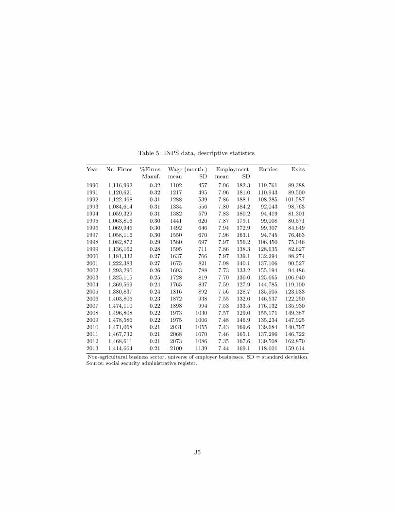
Table 5: INPS data, descriptive statistics

Year Nr. Firms %Firms Wage (month.) Employment Entries ExitsManuf. mean SD mean SD

1990 1,116,992 0.32 1102 457 7.96 182.3 119,761 89,3881991 1,120,621 0.32 1217 495 7.96 181.0 110,943 89,5001992 1,122,468 0.31 1288 539 7.86 188.1 108,285 101,5871993 1,084,614 0.31 1334 556 7.80 184.2 92,043 98,7631994 1,059,329 0.31 1382 579 7.83 180.2 94,419 81,3011995 1,063,816 0.30 1441 620 7.87 179.1 99,008 80,5711996 1,069,946 0.30 1492 646 7.94 172.9 99,307 84,6491997 1,058,116 0.30 1550 670 7.96 163.1 94,745 76,4631998 1,082,872 0.29 1580 697 7.97 156.2 106,450 75,0461999 1,136,162 0.28 1595 711 7.86 138.3 128,635 82,6272000 1,181,332 0.27 1637 766 7.97 139.1 132,294 88,2742001 1,222,383 0.27 1675 821 7.98 140.1 137,106 90,5272002 1,293,290 0.26 1693 788 7.73 133.2 155,194 94,4862003 1,325,115 0.25 1728 819 7.70 130.0 125,665 106,9402004 1,369,569 0.24 1765 837 7.59 127.9 144,785 119,1002005 1,380,837 0.24 1816 892 7.56 128.7 135,505 123,5332006 1,403,806 0.23 1872 938 7.55 132.0 146,537 122,2502007 1,474,110 0.22 1898 994 7.53 133.5 176,132 135,9302008 1,496,808 0.22 1973 1030 7.57 129.0 155,171 149,3872009 1,478,586 0.22 1975 1006 7.48 146.9 135,234 147,9252010 1,471,068 0.21 2031 1055 7.43 169.6 139,684 140,7972011 1,467,732 0.21 2068 1070 7.46 165.1 137,296 146,7222012 1,468,611 0.21 2073 1086 7.35 167.6 139,508 162,8702013 1,414,664 0.21 2100 1139 7.44 169.1 118,601 159,614

Non-agricultural business sector, universe of employer businesses. SD = standard deviation.Source: social security administrative register.

35