Tax Rate Variability and Public Spending asSources of Indeterminacy

Teresa Lloyd-Braga1, Leonor Modesto2∗and Thomas Seegmuller31Universidade Católica Portuguesa (UCP-FCEE) and CEPR2Universidade Católica Portuguesa (UCP-FCEE) and IZA

3CES and CNRS

January 25, 2006

AbstractWe consider a constant returns to scale, one sector economy with

segmented asset markets, encompassing both theWoodford (1986) andoverlaping generations models. We analyze the role of public spend-ing, financed by (labour or capital) income and consumption taxation,on the emergence of indeterminacy. We find that what is relevant forindeterminacy is the variability of the distortion introduced by gov-ernment intervention. We further discuss the results in terms of thelevel of the tax rate, its variability with respect to the tax base and thedegree of externalities in preferences due to the existence of a publicgood. We show that the degree of public spending externalities affectsthe combinations between the tax rate and its variability under whichindeterminacy occurs. Moreover, in contrast to previous results, wefind that consumption taxes can lead to local indeterminacy whenasset markets are segmented.

Keywords: Indeterminacy, public spending, taxation, segmented asset mar-kets.

JEL Classification: E32, E63, H23.∗Corresponding Author: correspondence should be sent to Leonor Modesto, Univer-

sidade Católica Portuguesa, FCEE, Palma de Cima, 1649-023 Lisboa, Portugal. e-mail:lrm@fcee.ucp.pt.

1

1 IntroductionThe effects of government spending and taxes on income distribution, eco-nomic growth and welfare have been thoroughly discussed in the literature.More recently some papers have also stressed that fiscal policy may cre-ate indeterminacy, and thereby have destabilizing effects on the economyby triggering expectations driven cycles, i.e. sunspots. The pioneer workof Schmitt-Grohé and Uribe (1997) shows that, in a Ramsey model with apre-set level of government expenditures, when the labor income tax is deter-mined by a balanced budget rule, the economy can exhibit an indeterminatesteady state and a continuum of stationary sunspot equilibria. Gokan (2005)and Pintus (2003), considering the same fiscal policy rule, show that similarresults are obtained in a segmented asset market economy of the Woodford(1986) type.In this paper we extend this analysis, studying the role of public spending

financed by taxation on the emergence of indeterminacy, within segmentedasset markets economies, for a wider class of fiscal policy rules. We considera general unified structure that encompasses two types of segmented assetmarkets economies with a constant returns to scale Cobb-Douglas technology,the Woodford (1986) and the overlapping generations (OLG) economy as de-veloped in Reichlin (1986). We further show that a Woodford economy withgovernment spending financed by labor income and/or consumption taxationis isomorphic to a Reichlin framework with government spending financed bycapital income and/or consumption taxes. In both cases the government in-tervention only introduces a multiplicative (endogenously variable) distortionin the equilibrium intertemporal choice of agents between consumption andleisure, which does not affect the capital accumulation equation. The maindifference between these two frameworks lies on the values assumed for thedepreciation rate: high in the overlapping generations model and small inthe Woodford (1986) framework.1

It is well known that constant income tax rates can not be per se asource of local indeterminacy in a Ramsey model.2 The same happens in asegmented asset market economy as proved below. Therefore, we focus onvariable tax rates, i.e. tax rates that vary (negatively or positively) with thetax base, while government spending adjusts in order to balance the budget.

1This is due to the fact that in the OLG model agents live for two periods, whereas inthe Woodford (1986) framework they are infinitely lived.

2See Schmitt-Grohé and Uribe (1997) and Guo and Harrison (2004).

2

The tax rate rule considered is characterized by two parameters: the levelof the tax rate and its variability with respect to the tax base.3 Our fiscalpolicy rule covers as particular cases those considered in Schmitt-Grohé andUribe (1997), Pintus (2003), Dromel and Pintus (2004), Giannitsarou (2005)and Gokan (2005), and also the case of a constant tax rate.Moreover, we also introduce the possibility of government spending ex-

ternalities in preferences.4 We study how the degree of government spendingexternalities affects the combinations between the tax rate and its variability,under which indeterminacy occurs. For example, we find that in the absenceof government spending externalities, for a fixed positive response of the taxrate to the tax base, a sufficiently low tax rate ensures determinacy. However,this is no longer true for higher values of public spending externalities. Also,with constant income tax rates, indeterminacy becomes possible when publicspending externalities on preferences are sufficiently strong in the Woodfordframework, or even with arbitrarily small externalities in the OLG model.Therefore, our results show that taking into account (and accurately mea-suring) the degree of government spending externalities is crucial in order tocorrectly evaluate the dynamic implications of different fiscal policy rules.Another novel feature of our work is that we study the effects of con-

sumption taxation on indeterminacy in segmented asset markets economies.Giannitsarou (2005), using a Ramsey model, addressed only the case where afixed stream of government spending is financed by consumption taxes, andfound that indeterminacy was not possible in this case. Here, we considera more general fiscal policy rule that encompasses the one analyzed in Gi-annitsarou (2005). We find that, in a segmented asset markets framework,indeterminacy is possible with a consumption tax rate that responds nega-tively to the tax base. In particular, in the case analyzed in Giannitsarou(2005) indeterminacy may emerge, even without public spending externalitieson preferences. This shows that taxes have different effects on indeterminacyin segmented asset markets and Ramsey models. Being aware of the markets’distortions (e.g. financial imperfections) existing in the pre intervention sit-

3The functional form considered for the tax rate is similar the one used by Guo andLansing (1998), although the tax bases are different.

4Seegmuller (2003) analyzes the role of this type of externalities in OLG economies,but he only considers constant tax rates. Cazzavillan (1996), using an optimal growthmodel again with constant tax rates, introduces not only public spending externalities inpreferences but also in production. Note however that the latter also distort the capitalaccumulation equation.

3

uation is therefore also crucial to address correctly the dynamic implicationsof fiscal policy rules.Finally let us remark that one advantage of considering an unified frame-

work to analyze the role of public spending financed by taxation on indeter-minacy in segmented asset markets is that, by doing so, we are able to seevery clearly that quite different fiscal policies in sufficiently different modelsshare the same indeterminacy mechanism. Indeed, we find that, both in theWoodford and OLG frameworks, and for both income and consumption tax-ation, indeterminacy depends on the variability of the distortion introducedby government intervention. In the Woodford framework, indeterminacy re-quires a sufficiently strong variability of the distortion, whereas in the OLGframework, this variability can be arbitrarily small.The rest of the paper is organized as follows. In the next section, we

present a general unified framework of a segmented asset markets economythat admits as particular cases both theWoodford (1986) model and the OLGeconomy studied by Reichlin (1986) with a public sector. We then analyze thesteady state and derive the conditions for the emergence of indeterminacy inthis framework. In section 3, we extend the Woodford (1986) model to allowfor public spending, that may affect preferences and is financed by labor andconsumption taxes. Then, in section 4, we present and discuss in detail theindeterminacy results in the Woodford model considering labor income andconsumption taxes. In sections 5 and 6, we respectively present the OLGmodel with government spending and discuss its stability properties in thecases of capital income and consumption taxes. Finally, in the last section,we provide some concluding remarks.

2 The General FrameworkWe consider a one sector perfectly competitive economy with segmented assetmarkets and discrete time t = 1, 2, ...,∞, where both capital kt and labourlt are used to produce the final good, yt, under a Cobb-Douglas technologywith constant returns to scale:

yt = kst l1−st (1)

where s ∈ (0, 1) represents the capital share in total income. Producersmaximize their profits. Since all markets are perfectly competitive, we obtain

4

the following expressions for the real wage and the real interest rate:

ωt = (1− s)kst l−st ≡ ω(kt, lt) (2)

ρt = sks−1t l1−st ≡ ρ(kt, lt) (3)

In what follows, instead of developing a particular model with segmentedasset markets based on the behavior of consumers, we just present two dy-namic equations without a priori microeconomic foundations. As we will seelater in Section 3 and Section 5, this reduced form admits as particular casesthe Woodford (1986) model as well as the overlapping generations frame-work developed by Reichlin (1986). At this stage, we just clarify that thefirst equation corresponds to the intertemporal choice of workers betweenfuture consumption and leisure, whereas the second one describes capitalaccumulation.Hence, we assume in this section that the perfect foresight intertemporal

equilibrium of this economy is a sequence (kt, lt) ∈ R++×(0, l̃), t = 1, 2, ....∞that, for a given k1 > 0, solves the two-dimensional dynamic system:

(1− µ)yt+1ϕ(kt+1, lt+1)/B = γ (lt) (4)

kt+1 = β [(1− δ)kt + µyt] (5)

where B > 0 is a scaling parameter, µ ∈ (0, 1) is a constant and yt is given by(1). Moreover, both parameters β and δ belong to (0, 1], and γ (l) is a positivecontinuous function, differentiable as many times as needed for l ∈ [0, l̃],5 suchthat εγ(l) ≡ γ0(l)l/γ(l) ≥ 1. Finally, the function ϕ(k, l) summarizes theeffect of government intervention on this economy. On the function ϕ(k, l)we further assume that it is continuous for (k, l) ∈ R+ × [0, l̃], positivelyvalued and differentiable as many times as needed for (k, l) ∈ R++ × (0, l̃).Moreover, εϕx(k, l) ≡ ∂ϕ(k,l)

∂xx

ϕ(k,l)∈ R, with x ∈ {k, l}. In the absence of

government intervention ϕ(k, l) = 1, so that εϕx(k, l) = 0 for x ∈ {k, l}.One can also notice that while kt is a variable determined by past actions,

the value of lt, on the contrary, is affected by expectations of future events.Therefore, equations (4) and (5) determine the dynamics of the economy,through a two-dimensional dynamic system with one predetermined variable,the capital stock kt.

5The labor endowment l̃ may be finite or infinite.

5

As we will explain in Sections 3 and 5, equations (4) and (5) describethe dynamics of a Woodford economy for µ = s and δ < 1, whereas theysummarize the overlapping generations behavior for µ = 1 − s, δ = 1 andβ = 1.

2.1 Steady State Analysis

In this section, we establish conditions for the existence of a unique steadystate (k, l) of the dynamic system (4) and (5).

Proposition 1 Existence and uniqueness of the steady state:Defining H(l) ≡ lϕ(a∗l, l)/γ(l), a∗ = (µβ/θ)1/(1−s) and θ ≡ 1−β(1−δ) ∈

(0, 1], and assuming that (1 − µ)(a∗)smax{liml→0H(l), liml→elH(l)} < B <(1−µ)(a∗)smin{liml→0H(l), liml→elH(l)}, the dynamic system (4)-(5) has aunique steady state (k, l) if one of the two following conditions is satisfied:

1. Either 1 + εϕk(a∗l, l) + εϕl(a

∗l, l) > εγ(l) for l ∈ (0, l̃)2. or 1 + εϕk(a

∗l, l) + εϕl(a∗l, l) < εγ(l) for l ∈ (0, l̃)

Proof. Studying the existence and uniqueness of the steady state (k, l)of the dynamic system (4) and (5) is equivalent to analyze the existence anduniqueness of a stationary solution (a, l), with a ≡ k/l, of the two followingequations:

µas−1 = θ/β (6)

(1− µ)aslϕ(al, l)/B = γ(l) (7)

We can easily see that a∗ is the unique solution to equation (6). Since H(l)is a continuous function, under the boundary assumptions on B stated inProposition 1, there exists a value l∗ solving (7) with a = a∗. Uniqueness ofl∗ is ensured by inequalities 1 or 2 , because in these casesH(l) is a monotonicfunction.

6

2.2 Indeterminacy

Assuming that Proposition 1 is verified, we now study the local indeterminacyof the steady state. To do so, we differentiate the two-dimensional dynamicsystem (4) and (5) in the neighborhood of the steady state. The trace T andthe determinant D of the associated Jacobian matrix are given by:

T = 1 +εγ − θ(1− s)(1 + εϕl + εϕk)

εϕl + 1− s(8)

D =εγ [1− θ(1− s)]

εϕl + 1− s(9)

where εγ ≥ 1, εϕk and εϕl denote respectively the elasticities εγ(l), εϕk(k, l)and εϕl(k, l) evaluated at the steady state.We summarize our results in Proposition 2 below.

Proposition 2 IndeterminacyThe steady state will be indeterminate if and only if one of the following

conditions is satisfied:(i) εϕl > max

©εTϕl, ε

Hϕl, ε

Fϕl

ª;

(ii) εϕl < min©s− 1, εTϕl, εFϕl

ª;

where:εTϕl = −εϕk + (εγ − 1)εHϕl = [s− θ(1− s)] + [1− θ(1− s)] (εγ − 1)εFϕl = − [

4−2s−θ(1−s)(2+εϕk)]2−θ(1−s) − (εγ − 1).

Proof. Since we only have one predetermined variable (capital) thesteady-state is locally indeterminate when it is a sink (both eigenvalues withmodulus lower than one). Therefore indeterminacy requires that D < 1,1 − T + D > 0 and 1 + T + D > 0. When the denominator of both thetrace and the determinant is positive (εϕl > s − 1) these conditions can bewritten respectively as εϕl > εHϕl, εϕl > εTϕl, and εϕl > εFϕl where ε

Hϕl, ε

Tϕl and

εFϕl are given in Proposition 2. When the denominator of both the trace andthe determinant is negative (εϕl < s − 1) these conditions can be writtenrespectively as εϕl < εHϕl, εϕl < εTϕl, and εϕl < εFϕl. Combining these results,and noticing that εHϕl > s− 1, Proposition 2 immediately follows.

7

Note that, in this framework, it is not the level of the distortion introducedby government intervention per se that is responsible for the emergence ofindeterminacy, but its variability (εϕk 6= 0, εϕl 6= 0). Indeed when εϕk =εϕl = 0, we can see from Proposition 2 that the steady state can never beindeterminate. For instance, when εϕk = 0, from (i) of Proposition 2 we havethat εϕl > (εγ − 1) ≥ 0 is a necessary condition for indeterminacy, and from(ii) it is necessary that εϕl < s−1 < 0 for indeterminacy to emerge. However,when θ ∈ (0, 1] is sufficiently high, indeterminacy is possible with arbitrarilysmall values for the elasticities εϕk and εϕl. Consider that εγ = 1. In thiscase, when θ is sufficiently close to 1, such that θ(1− s) > s, εHϕl is negative.Moreover, with εϕk arbitrarily small, εFϕl is also negative. Therefore, condition(i) of Proposition 2 becomes in this case εϕk+ εϕl > 0, which can be satisfiedwith arbitrarily small positive values for εϕl and εϕk. On the contrary, whenθ is small, i.e. θ(1 − s) < s, εHϕl is positive, so that condition (i) requiresa positive value for εϕl bounded away from zero. Since from condition (ii)εϕl must take a negative value bounded away from zero (εϕl < s − 1 < 0)we conclude that indeterminacy is not possible for arbitrarily small values ofεϕk and εϕl when θ is small. For future reference we summarize this resultin Corollary 1. Let us define

ϕ ≡ εϕk + εϕl (10)

Then we can state:

Corollary 1Assuming εγ = 1 and εϕk arbitrarily small, indeterminacy can arise for

any ϕ > 0 if and only if θ(1− s) > s.

3 The Woodford (1986) Model with Govern-ment Spending

In this section we apply the general framework developed above to the caseof a Woodford (1986) model extended to allow for public spending financedby taxation. We consider a perfectly competitive monetary economy withdiscrete time t = 1, 2, ...,∞ and heterogeneous infinite lived agents. Indeed,following Woodford (1986), we assume that there are two types of agents,workers and capitalists. While workers and capitalists consume both the fi-nal good, only workers supply labour. Moreover, there is a financial market

8

imperfection that prevent workers from borrowing against their wage incomeand workers are more impatient than capitalists, i.e. they discount the fu-ture more than the latter. So, in a neighborhood of a monetary steady state,capitalists hold the whole capital stock and no money, whereas workers savetheir wage earnings through money balances. As before the final good is pro-duced by firms under a Cobb-Douglas technology characterized by constantreturns to scale. Finally, we introduce government policy in this framework,and assume that public spending, that may affect workers utility, is financedby labour and/or consumption taxes. The detailed description of the modelis provided below. We further show that this economic environment is noth-ing more than a special case of the general framework presented before and,therefore, we apply our previous results summarized in Proposition 2 to thediscussion of indeterminacy in this case.

3.1 The Government

The government chooses the tax policy and balances its budget at each periodin time. Therefore, real public spending in goods and services in period t,Gt ≥ 0 is given by:

Gt = τ (ωtlt)ωtlt + τ (ct) ct (11)

where τ (ωtlt) represents the labour tax rate determined as a function ofaggregate labour income in the economy. Also ct = cwt + cct , where c

wt denotes

consumption of workers in period t, cct denotes consumption of capitalistsin period t and τ (ct) represents the consumption tax rate determined as afunction of aggregate consumption. We assume that:

τ (ωtlt) = αl

µωtltωl

¶φl

(12)

τ (ct) = αc

³ctc

´φc(13)

where ωl is the steady state value of the wage bill and c is the steady statelevel of total consumption. The parameter 0 ≤ αl < 1 determines the levelof the tax rate on labour income at the steady state. Similarly αc ≥ 0determines the level of the consumption tax rate at the steady state. Theparameters φj with j = l, c denote the elasticities of the tax rates withrespect to the tax bases. When φj < 0 the tax rate decreases when the taxbase expands. φj > 0 corresponds to the cases where the tax rate increases

9

with the tax base, and for φj = 0 the tax rate is constant. The specificationconsidered for the fiscal policy rule given by (11), (12) and (13) is quitegeneral, and nests most of the cases considered in the literature. Indeed itis similar to the specification considered by Guo and Lansing (1998). It alsonests the case considered in Schmitt-Grohé and Uribe (1997), Pintus (2003)and Gokan (2005) where a constant amount of public expenditures is financedby taxes on labour income, so that. τ t = G/ωtlt. Hence we recover theirspecification when φl = −1 and αc = 0. Moreover, we admit as a particularcase Giannitsarou (2005) for αl = 0 and φc = −1, which means that constantpublic expenditures are only financed by consumption taxes.

3.2 Workers

We assume a continuum of identical workers of mass one. Preferences of eachworker may be affected by public expenditures and are represented by thefollowing utility function:

∞Xt=1

λt−1·U

µGηt c

wt

B

¶− λV (lt)

¸(14)

where lt is labor supply, cwt is his consumption, and λ ∈ (0, 1) is the discountfactor. Public spending externalities in preferences are given by Gη whereη ≥ 0 represents the degree of these externalities. Moreover, we make thefollowing assumptions on the utility functions U and V :

Assumption 1 The functions U (x) and V (l) are continuous for all x ≥ 0and 0 ≤ l ≤ el, where the labor endowment el > 0 may be finite or infinite.They are Cn for x > 0, 0 < l < el and n large enough, with U 0(x) > 0,U 00(x) ≤ 0, V 0(l) > 0 and V 00(l) ≥ 0. Moreover, liml→elV 0(l) = +∞ andconsumption and leisure are gross substitutes, i.e. −xU 00(x)/U 0(x) < 1.

In the following mwt+1 and kwt+1 denote respectively the money balances

and the capital stock held by the representative worker at the end of periodt, δ ∈ (0, 1) is the depreciation rate of capital, rt the nominal interest rate,wt the nominal wage, and pt the price of the final good. At each period, aworker faces the two following constraints:

ptcwt (1+ τ (ct))+pt

¡kwt+1 − (1− δ)kwt

¢+mw

t+1 = mwt +rtk

wt +(1−τ(ωtlt))wtlt

(15)

10

ptcwt (1 + τ (ct)) + pt

¡kwt+1 − (1− δ)kwt

¢ ≤ mwt + rtk

wt (16)

where (15) represents the budget constraint and (16) the liquidity constraint.The representative worker maximizes his utility function (14) under the con-straints (15) and (16). Workers know the policy rule followed by the gov-ernment. However, since there is a continuum of agents, each worker, beingatomistic, does not take into account the influence of its actions on aggregatevariables. This means that workers take Gt, τ (ct) and τ (ωtlt) as given whensolving their maximization problem. The equilibria considered here are suchthat:

GηtU

0µGηt c

wt

B

¶> λGη

t+1U0µGηt+1c

wt+1

B

¶[(1− δ) + rt+1/pt+1] (17)

(1− δ)pt+1 + rt+1 > pt (18)

Then, workers always choose kwt = 0 and the finance constraint is binding.Therefore, we obtain the following equations:

u

µGηt+1c

wt+1

B

¶= v(lt) (19)

mwt+1 = (1− τ (ωtlt))wtlt (20)

ptcwt (1 + τ (ct)) = mw

t (21)

where u(x) = xU 0(x) and v(z) = zV 0(z). We can further notice that underAssumption 1, it exists a function γ ≡ u−1 ◦ v, such that Gη

t+1cwt+1/B = γ(lt)

and εγ(l) ≡ γ0(l)l/γ(l) ≥ 1.

3.3 Capitalists

Capitalists behave like a representative agent who maximizes his lifetimeutility function:

∞Xt=1

βt ln cct (22)

11

where β ∈ (λ, 1) is his discount factor and cct his consumption.6 At period t,

the representative agent faces the following budget constraint:

ptcct(1 + τ (ct)) + pt

¡kct+1 − (1− δ)kct

¢+mc

t+1 = mct + rtk

ct (23)

where mct+1 and kct+1 are respectively the money balances and the capital

stock held at the end of period t by capitalists. Since we focus on equilibriasatisfying (18), capitalists do not hold money (mc

t = 0) because it has a lowerreturn than capital. We obtain then, the following optimal solution:

cct =(1− β)Rtkt1 + τ (ct)

(24)

kt+1 = βRtkt (25)

where Rt ≡ 1− δ + rt/pt is the real gross return on capital.7

3.4 The Production Sector

As before we consider a constant returns to scale Cobb-Douglas technologyand perfectly competitive input markets. Producers maximize profits so thatequations (2) and (3) apply.

3.5 Equilibrium

Equilibrium on labor and capital markets requires ωt = wt/pt, ρt = rt/pt.Considering that m > 0 is the constant money supply, and using (20) and(21), equilibrium in the money market at each period implies the following:

m/pt = (1 + τ (ct))cwt = (1− τ(ωtlt))ωtlt (26)

Therefore, at equilibrium (19) and (25) become:

ωt+1lt+1Gηt+1(1− τ (ωt+1lt+1))

B(1 + τ (ct+1))= γ (lt) (27)

6We do not introduce public expenditures externalities into capitalists preferences be-cause, since they have a log-linear utility function, such externalities would not affect thedynamics.

7The superscript on kct is dropped because as we have seen before, workers do not holdcapital.

12

kt+1 = β [ρt + 1− δ] kt (28)

where ωt and ρt satisfy respectively (2) and (3), Gt, τ (ωtlt) and τ (ct) aregiven respectively by (11), (12) and (13), and ct = cwt + cct , where c

wt and cct

satisfy respectively (26) and (24).Equations (27) and (28) determine the dynamics of this economy, through

a two-dimensional dynamic system with one predetermined variable, the cap-ital stock kt. Comparing these two last equations with (4) and (5) we can seethat the Woodford (1986) economy with public spending, financed by labourand consumption taxes, is a special case of the general framework studied insection 2, with µ = s, δ < 1 and

ϕ(kt+1, lt+1) = [Gηt+1(1− τ(ωt+1lt+1)]/(1 + τ (ct+1)) (29)

Therefore, to study indeterminacy in this economy we can merely applyProposition 2. That is precisely what we do in the next section, where,for simplicity of exposition, we consider separately the cases of labour andconsumption taxes.Remark that the distortion function ϕ can be decomposed in two factors.

The distortion due to government spending externalities is given byGη, while(1 − τ (ωl))/(1 + τ (c)) represents the gap between real wages relevant toconsumers and producers, due to taxation (the tax wedge). Of course thefunctional form of the distortion function ϕ(k, l) and its variability dependon the chosen fiscal policy rule and its parameters. However, as we shallsee, for the class of policy rules here considered, and in both the Woodfordand OLG frameworks, we are able to summarize in one single parameter theinfluence of the policy rule on the distortion variability.Finally, note that in the absence of government intervention, i.e. when

ϕ(k, l) = 1, (27) and (28) describe the dynamics of the standard Woodford(1986) model studied in Grandmont et al. (1998).

4 Indeterminacy in theWoodfordModel withGovernment Spending

In this section, we analyze indeterminacy in the Woodford model assumingthat θ is small, i.e. s − θ(1 − s) > 0. Note that this assumption is fre-quently used in the literature (see Cazzavillan et al. (1998)) and covers most

13

commonly used parameterizations for the Woodford model.8

4.1 Indeterminacy with Labour Taxation

In this section we discuss in detail the case where only labour taxation isused to finance public spending, i.e. where αc = 0 so that τ (ct) = 0, see(13). In this case (11) and (29) become

Gt+1 = τ (ωt+1lt+1)ωt+1lt+1 (30)

ϕ(kt+1, lt+1) = Gηt+1(1− τ (ωt+1lt+1)) (31)

where τ (ωl) satisfies (12). Therefore we obtain

εϕl =

·η(1 + φl)− φl

αl

1− αl

¸(1− s) (32)

εϕk =

·η(1 + φl)− φl

αl

1− αl

¸s (33)

so that ϕ (see (10)) is given by:9

ϕ =

·η(1 + φl)− φl

αl

1− αl

¸(34)

Government policy affects the economy through the parameters η, φl andαl: η(1 + φl) represents the variability of the public spending externality onpreferences,10 while φl

αl1−αl represents the variability of the tax wedge. These

parameters only influence εϕl and εϕk through a single factor ϕ. Hence ϕ

summarizes the variability of the distortion introduced by fiscal policy.We now derive the indeterminacy conditions corresponding to the labour

taxation case. In order to make the analysis comparable to the existingliterature we set γ = 1.11 We summarize our results in Proposition 3 below.

8Indeed most quarterly parameterizations assume θ close to 0.025.9Note that here ϕ represents also the elasticity of the function ϕ with respect to the

tax base (the wage bill), evaluated at the steady state.10When φl = −1 the variability of the public spending externality disappears because

G is constant.11Note that this corresponds to the case of an infinitely elastic labour supply curve.

14

Proposition 3 Indeterminacy under labour taxation and public ex-penditures externalities in the Woodford model:Assuming that θ(1 − s) < s and γ = 1, the steady state will be indeter-

minate if and only if:(i) for αl < η/(1 + η) either φl > φHl or φl < φFl(ii) for αl > η/(1 + η) either φl < φHl or φl > φFlwhere:

φHl =(1− αl) [s− θ(1− s)− η(1− s)]

(1− s) [η − αl(1 + η)]

φFl =−(1− αl) {2 [2− s− θ(1− s)] + η(1− s)(2− θ)}

(1− s)(2− θ) [η − αl(1 + η)]

Proof. Since this a special case of the general one presented in section2, Proposition 2 applies. Using expressions (32) to (34), it is easy to showthat, for γ = 1, conditions (i) and (ii) of Proposition 2 can be written as

ϕ > maxn0, [s−θ(1−s)]

(1−s) , −2[2−s−θ(1−s)](2−θ)(1−s)

oand ϕ < min

n−1, 0, −2[2−s−θ(1−s)]

(2−θ)(1−s)o.

Since, for θ(1 − s) < s, [s−θ(1−s)](1−s) = max

n0, [s−θ(1−s)]

(1−s) , −2[2−s−θ(1−s)](2−θ)(1−s)

oand

−2[2−s−θ(1−s)](2−θ)(1−s) = min

n−1, 0, −2[2−s−θ(1−s)]

(2−θ)(1−s)o, these two conditions become re-

spectively ϕ > [s−θ(1−s)](1−s) and ϕ < −2[2−s−θ(1−s)]

(2−θ)(1−s) . Then, using expression (34)to substitute ϕ in these two last inequalities, it is straightforward to obtainProposition 3.

From this proof we can see that indeterminacy is more likely the higherthe (absolute) value of ϕ, i.e. the stronger the variability of the distortion.

4.1.1 Economic Intuition

In our framework the distortion introduced by government intervention is themechanism responsible for the emergence of indeterminacy, which requiresa sufficiently strong variability of the function ϕ. Indeed, in the absence ofgovernment spending financed by taxation, i.e. when ϕ = 0 so that εϕl = 0and εϕk = 0, we recover the case considered in Grandmont et al. (1998),where the steady state is never indeterminate in the Cobb-Douglas case.In order to understand why, consider the following intuitive argument that,since local indeterminacy is closely related to the existence of deterministic

15

and/or stochastic fluctuations, is based on the existence of a mechanismgenerating cyclical equilibrium trajectories. Consider for instance that inperiod t, starting from the steady state, there is an instantaneous increase inthe capital stock kt. Agents anticipate that this implies an increase in kt+1(see (28)), and therefore in the future wage bill. In the absence of publicspending financed by labour taxation this expected increase in the futurewage bill must be sustained by an increase in current employment, see (27),which in turn implies an increase in the current interest rate (see (3)), thatreinforces the initial increase in kt+1. This in turn implies a decrease in therental rate of capital at t + 1. In order to obtain a cyclical trajectory asufficiently important decrease in the rental rate of capital at t + 1 shouldbe observed, so that kt+2 decreases. However, in the Cobb-Douglas case thiscan never happen so that indeterminacy never emerges.Consider now the case where ϕ > 0, i.e. where we have tax rates that

respond negatively to the tax base (φ < 0) and/or public spending external-ities (η > 0). See equation (34). Now, the anticipated increase in the futurewage bill implies a stronger increase in current employment (see (27)), whichreinforces all the events described above, leading, if ϕ is sufficiently big, toa sufficiently fall in rt+1, that reverses the trajectory of capital.Assume now that ϕ < 0, i.e. taxes vary positively with the tax base

(φ > 0). Then, if ϕ is sufficiently big in absolute value, the anticipatedincrease in the future wage bill may, in contrast to what happened in the twoprevious cases, lead to a decrease in current employment. See equation (27).This last effect has a negative impact on the current interest rate (see (3)),which reduces kt+1 restoring the path to equilibrium.We can therefore understand why the emergence of indeterminacy re-

quires sufficiently high (in absolute terms) values for ϕ , i.e. a sufficientlyelastic response of the function ϕ with respect to capital and labor.

4.1.2 Discussion of the Results

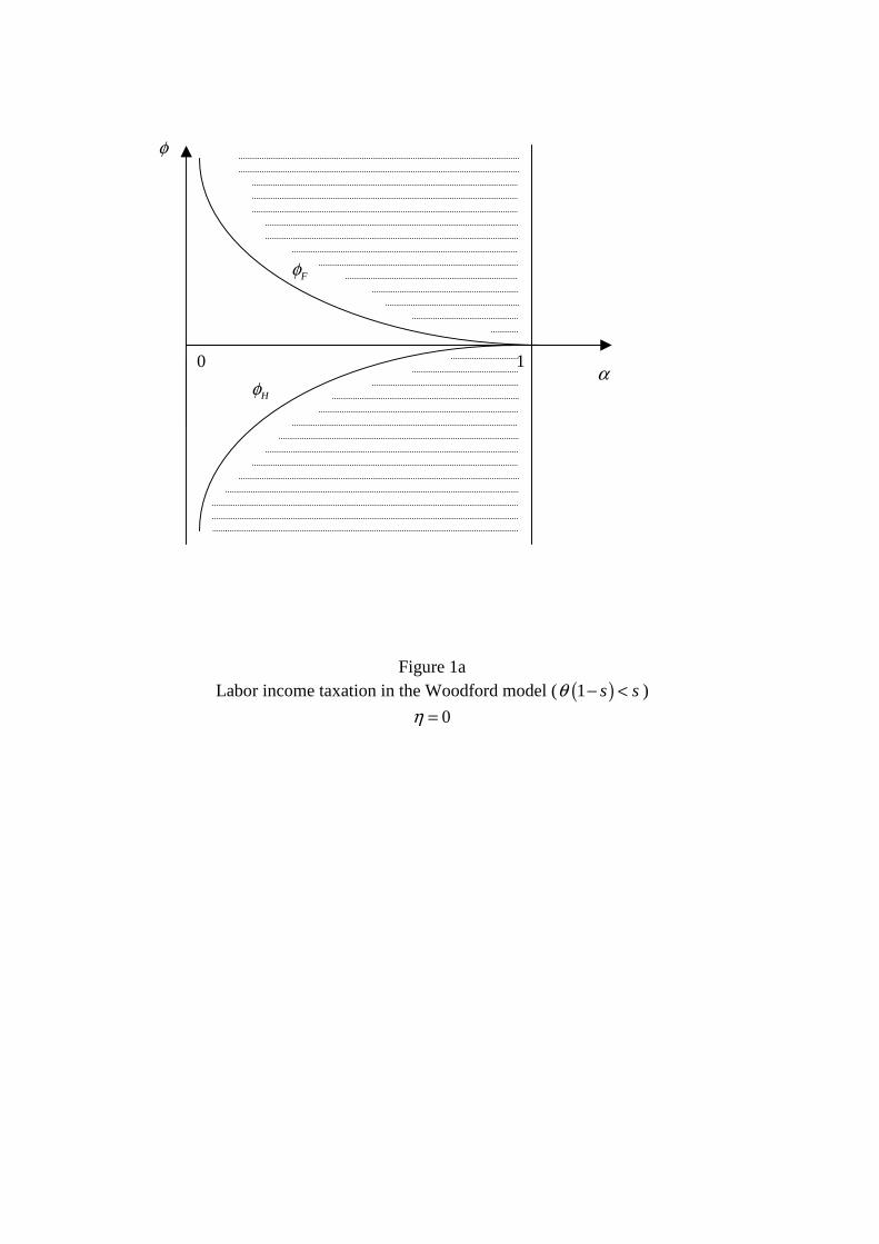
In this section we discuss and compare our indeterminacy results with pre-vious papers that have addressed the same issue. To ease the discussion wehave plotted, in figure 1, φHl and φFl as functions of 0 < αl < 1 for differentvalues of η ≥ 0, assuming that θ(1− s) < s.

(insert figures 1a, 1b and 1c here)

The case of η = 0, where public spending does not affect workers’ utility,

16

falls into case (ii) of Proposition 3 and is depicted in figure 1a. We cansee that, in this case, indeterminacy is not possible with a constant tax rate(φl = 0).12 The same result was obtained in a Ramsey model by Schmitt-Grohé and Uribe (1997) and Guo and Harrison (2004). However, for anygiven level of αl, a sufficiently (positively or negatively) elastic tax rule impliesthe existence of indeterminacy. In this respect our results are in contrast withthose obtained in Guo and Lansing (1998) or Dromel and Pintus (2004).Indeed, in the Benhabib and Farmer (1994) framework, Guo and Lansing(1998) find that saddle path stability is more likely when the tax schedulebecomes more progressive. More recently, Dromel and Pintus (2004), in aWoodford model without government spending externalities, also find that asufficiently progressive tax rate on labor income promotes determinacy. Notethat both Guo and Lansing (1998) and Dromel and Pintus (2004) restricttheir analysis to the case of weak progressivity. In fact, since in their caseagents take into account how the tax rate affects their earnings, they haveto exclude parameter configurations where after tax income decreases withincome, i.e., where ϕ < −1 or φl > (1 − αl)/αl(< φFl ) in our notation.On the contrary, in our case, since agents take the tax rate as given, theseparameter configurations are possible.From figure 1a we can also see that, for a given level of φl 6= 0, in-

determinacy requires a sufficiently high level of αl. In particular, when aconstant level of G is assumed (φl = −1), local indeterminacy emerges whenαl > [s− θ(1− s)] / [1− θ(1− s)].13 This result is in accordance with pre-vious works considering labor taxation and no public expenditures external-ities. See for instance Schmitt-Grohé and Uribe (1997), Pintus (2003) andGokan (2005) who assume a constant level of G and all find that indetermi-nacy requires a lower bound for the tax rate.We can therefore conclude that for a given value of φl, a sufficiently low

level of the tax rate stabilizes economic fluctuations, whereas for a given levelof the tax rate, αl, tax schedules sufficiently elastic destabilize the economy.This means that there is a trade-off between the values of these two para-meters, φl, the tax response to the business cycle and αl, the level of taxrate, needed for determinacy: the higher the elasticity of the tax schedule,the lower the tax rate needed to ensure determinacy of the steady state.

12Note that, when η = 0, the case of a constant tax rate is equivalent to the case whereεϕl = εϕk = 0 (see (32) to (34)), so that, as shown before, indeterminacy is not possible.13When φl = −1, we obtain this same indeterminacy condition on αl for any value of

η ≥ 0, because the effect of the public spending externality disappears when G is constant.

17

When η > 0 two different configurations are possible depending on whetherη ≷ [s− θ(1− s)] /(1 − s). In figure 1b we represent the case where η <[s− θ(1− s)] /(1 − s). We can see that, in this case, indeterminacy is stillnot possible with a constant tax rate (φl = 0). However, for low values ofαl, a new type of configuration, that reverses the trade-off between αl andφl needed for determinacy, is obtained: the higher φl, the higher the value ofαl required for determinacy.Finally the case of higher public spending externalities, η > [s− θ(1− s)]

/(1 − s), is represented in figure 1c. We can see that, in this case, inde-terminacy prevails for φl ≥ 0 and αl < η/(1 + η), and for φl ≤ 0 andαl > η/(1+ η). In particular, and in contrast to what happened in the othertwo previous cases, indeterminacy is now always obtained with a constanttax rate (φl = 0).14 Cazzavillan (1996), in an optimal growth model withpublic spending externalities on preferences and production and a constanttax rate, also found that a minimum bound for the elasticity of the publicspending externalities was required for indeterminacy to emerge.15 These re-sults suggest that public expenditures externalities on preferences constitutean important channel for the emergence of indeterminacy.The results here obtained show that fiscal policy rules may be responsible

for indeterminacy, and thereby their design should take into account theirpossible destabilizing effects through this channel. This is an issue alreadyemphasized in several other works, but our results further show that the wayφl and αl interact in order to create local indeterminacy strongly dependson the presence and strength of public spending externalities. Therefore, inorder to design the ’correct’ policy rule we must estimate the existing degreeof public spending externalities in preferences, i.e. the value of η.

4.2 Indeterminacy with Consumption Taxes

We consider now that the government only uses consumption taxes, i.e. thatαl = 0 so that τ (ωtlt) = 0 (see (12)). To simplify the analysis, we ignore

14Indeed, when φl = 0, indeterminacy requires a minimum degree for public spendingexternalities in preferences, precisely η > [s− θ(1− s)] /(1− s). See Proposition 3.15In his case this required minimum bound is higher than ours. Note, however, that the

two models are considerably different. For related results in an OLG model, see Seegmuller(2003) and Utaka (2003).

18

public spending externalities in preferences, i.e. η = 0, so that (29) becomes:

ϕ(kt+1, lt+1) =1

1 + τ (ct+1)(35)

where τ (ct) is given by (13), and using (2), (3), (24) and (26) ct satisfies thefollowing equation:

(1 + τ (ct))ct = ωtlt + (1− β)Rtkt

= kt[(1− β)(1− δ) + (1− sβ)ks−1t l1−st ]. (36)

Accordingly we have that

εϕl =−αcφc

1 + αc(1 + φc)

·(1− s)(1− βs)θ

(1− s)θ + (1− β)s

¸(37)

εϕk =−αcφc

1 + αc(1 + φc)

·1− (1− s)(1− βs)θ

(1− s)θ + (1− β)s

¸(38)

so that ϕ (see (10)) is given by:16

ϕ =−αcφc

1 + αc(1 + φc)(39)

As in the case of labour taxation ϕ summarizes the variability of the distor-tion due to fiscal policy. Since η = 0, ϕ has only a term which representsthe variability of the tax wedge.We now derive the indeterminacy conditions corresponding to the con-

sumption taxation case that we summarize in Proposition 4 below. Again,in order to make the analysis comparable to the existing literature, we haveset γ = 1.

Proposition 4 Indeterminacy under consumption taxation in theWoodford model:16Note that here ϕ represents also the elasticity of the function ϕ with respect to

income used for consumption expenditures, evaluated at the steady state. One can alsoeasily determine the elasticity of the distortion with respect to the tax base, which is equalto −αcφc/(1 + αc).

19

Assuming that θ(1 − s) < s and that γ = 1, the steady state is indeter-minate if and only if φFc < φc < φHc for φc 6= −(1 + αc)/αc where:17

φHc = − v

(1 + v)

(1 + αc)

αc

< 0

φFc = − ρ

(ρ− 1)(1 + αc)

αc< 0

ν =[s− θ(1− s)] [(1− s)θ + (1− β)s]

(1− s)(1− βs)θ> 0

ρ =2 [2− s− θ(1− s)] [(1− s)θ + (1− β)s]

θ(1− s) [2− s− (1− s)θ − βs]> 1

Proof. The model of this section is a special case of the general one pre-sented in section 2, so that Proposition 2 applies. Using expressions (37) to(39), it is easy to show that, for γ = 1, conditions (i) and (ii) of Proposition 2

become respectively ϕ > max {0, ν,−ρ} and ϕ < minn− [(1−s)θ+(1−β)s]

(1−βs)θ , 0,−ρo.

Since for θ(1−s) < s ν = max {0, ν,−ρ} and -ρ = minn− [(1−s)θ+(1−β)s]

(1−βs)θ , 0,−ρo,

those conditions become respectively ϕ > ν and ϕ < −ρ. Then, substitutingexpression (39) in these last two inequalities, it is straightforward to obtainProposition 4.

From the proof of Proposition 4 we can immediately see that, as in thecase of labour taxation, indeterminacy requires a sufficiently strong (in ab-solute value) variability of the function ϕ. Indeed, with both types of taxationthe mechanisms operating are the same, so that both the requirements andthe intuition for the emergence of indeterminacy are similar. Therefore, theeconomic intuition provided in the previous section also applies in this case.There remains however a difference worth emphasizing. In the case of labourtaxation, and ignoring for the sake of simplicity public spending external-ities, positive (negative) values for ϕ are always associated with negative(positive) values for φ, whereas in the case of consumption taxes this is nolonger true. See equation (39).18 This explains why the indeterminacy re-

17Note that for φc = −(1 + αc)/αc steady state consumption is not well defined (see(36)).18Indeed a positive ϕ implies that −(1 + αc)/αc < φc < 0, and a negative ϕ means

20

sults expressed in terms of the tax rate and its variability are so different inthe cases of labor and consumption taxes.

(insert figure 2 here)

In figure 2 we have represented the indeterminacy region (shaded area) inthe plane (αc, φc), by plotting the functions −1+αcαc

, φFc , and φHc as functionsof αc considering, as before, s > θ(1 − s). We can see that indeterminacywith consumption taxes is only possible for φc < 0, so that a consumptiontax rate that is increasing in the tax base implies local determinacy. Also,when the tax rate is constant (φc = 0) the steady state is never locallyindeterminate, as in the case of labor taxation without government spend-ing externalities.19 In the context of a Ramsey model, Giannitsarou (2005)found that indeterminacy is not possible when a fixed stream of governmentspending is financed by consumption taxes. On the contrary, in our set up,indeterminacy is possible when government spending is constant. Indeed,this case is here recovered assuming that φc = −1, and, from figure 2, we cansee that in this case, and as in the case of labour taxation, indeterminacyemerges when αc is sufficiently high (αc > ν).The sharp difference between our results and those of Giannitsarou (2005)

shows that the effects of policy rules on indeterminacy crucially depend onthe finance market imperfections existing in the economy.

5 The OLG Model with Government Spend-ing

In this section, we show that, when the technology is Cobb-Douglas, the dy-namics of an overlapping generations economy with public spending financedthrough capital or consumption taxation are still described by equations (4)and (5) with µ = 1 − s, δ = 1 and β = 1, so that our general results onindeterminacy presented in Proposition 2 apply in the particular case whereθ ≡ 1− β(1− δ) = 1.

that either φc < −(1 + αc)/αc or φc > 0. However, when φc > 0, ϕ > −1, so that ϕ isnever below −ρ < −1. Therefore indeterminacy never emerges when φc > 0. See figure 2.19Indeed when φc = 0 we have that εϕl = εϕk = 0, so that indeterminacy does not

emerge.

21

We consider an OLGmodel with two-periods lived consumers that supplylabor in the first period, save through capital, and consume only in thesecond period of their life (ct+1). As before we introduce variable publicexpenditures, now financed by capital income and/or consumption taxationaccording to the following rule:

Gt = τ(ρtkt)ρtkt + τ (ct) ct (40)

with τ (ct) given by (13,) and τ(ρtkt) given by:

τ(ρtkt) = αk

µρtktρk

¶φk

(41)

where ρk represents capital income at the steady state, αk ∈ [0, 1) is thesteady state capital income tax rate, φk > 0 (< 0) means that the tax rateincreases (decreases) with the tax base, whereas φk = 0 corresponds to aconstant tax rate.Consumers’ preferences are represented by the following utility function:

U(Gηt+1ct+1/B)− V (lt) (42)

where the functions U (x) and V (l) satisfy Assumption 1. Assuming thatcapital totally depreciates after one period of use (δ = 1), each consumer,taking the tax policy of the government, τ (ρtkt) and τ (ct), and the pub-lic good externality as given, maximizes his utility under the two budgetconstraints:

kt+1 = ωtlt (43)

(1 + τ (ct+1)) ct+1 = (1− τ(ρt+1kt+1))ρt+1kt+1 (44)

The solution to this problem is given by (43) and:

Gηt+1(1− τ (ρt+1kt+1))ρt+1kt+1

(1 + τ (ct+1))B= γ(lt) (45)

where ct+1 satisfies (44).20

20Note that the OLG model presented above is equivalent to an infinite horizon modelwhere consumption is financially constrained by capital income. Indeed if agents maximize∞Pt=1

βt−1 [U(Gηt ct/B)− βV (lt)] subject to the usual resources constraint (1 + τ (ct)) ct +

kt+1 = ωtlt + (1 − τ(ρtkt))ρtkt and additionally to the following finance constraint(1 + τ (ct)) ct ≤ (1 − τ(ρtkt))ρtkt, the solution is still given by (43) and (45), if the fi-nance constraint is binding. This provides an additional explanation for the segmentedasset markets interpretation of the OLG model. For further details see Seegmuller (2005).

22

Using (1), (2), (3), (13), (40), (41) and (44), we see that (43) and (45)describe a dynamic system which is a particular case of (4)-(5) with µ = 1−s,δ = 1, β = 1, and ϕ (kt+1, lt+1) given by:

ϕ (kt+1, lt+1) =Gηt+1(1− τ(ρt+1kt+1))

1 + τ (ct+1)(46)

As a consequence, the general conditions for indeterminacy summarized inProposition 2, considering θ ≡ 1 − β(1 − δ) = 1, apply to the overlappinggenerations model with capital and/or consumption taxation, and publicspending externalities. Recall that the same general indeterminacy condi-tions also apply in the Woodford model. The only difference concerns theparameter θ that in the Woodford framework is assumed to be sufficientlysmall, while it takes the value one in the OLG framework considered.As in the Woodford (1986) case the distortion function ϕ (see (46)) can

be decomposed in two factors: Gη the distortion due to government spendingexternalities and (1−τ(ρk))/(1+τ (c)) the tax wedge between the real rentalrates relevant to consumers and producers.Finally, note that in the absence of government intervention, i.e. when

ϕ(k, l) = 1, (43) and (45) describe the dynamics of a standard OLG modelas in Reichlin (1986) and Cazzavillan (2001).

6 Indeterminacy in OLGEconomies with Pub-lic Spending

For simplicity of exposition, we will consider separately the cases of capitaland consumption taxes.

6.1 Indeterminacy with capital taxation

In this section we discuss the case where only capital income taxation isused to finance public expenditures in an OLG economy, i.e. where αc = 0so that τ (ct) = 0. (see (13)). In this case, (46) becomes ϕ (kt+1, lt+1) =Gηt+1(1−τ(ρt+1kt+1)) so that the elasticities of ϕ (k, l) with respect to capital

23

and labor are given by:

εϕl =

·η(1 + φk)− φk

αk

1− αk

¸(1− s) (47)

εϕk =

·η(1 + φk)− φk

αk

1− αk

¸s (48)

so that ϕ (see (10)) is given by:21

ϕ ≡·η(1 + φk)− φk

αk

1− αk

¸(49)

As in the Woodford model ϕ summarizes the variability of the distortionfunction ϕ due to government intervention.22

Using Proposition 2 for θ = 1, and assuming as before that γ = 1,the conditions for local indeterminacy in the overlapping generations modelwith capital income taxation, a balanced-budget rule and public spendingexternalities can be summarized as follows:

Proposition 5 Indeterminacy under capital taxation and public ex-penditures externalities in the OLG model (θ = 1):Assuming that s < 1/2 and γ = 1, the steady state will be locally inde-

terminate if and only if:(i) for αk < η/(1 + η) either φk > φTk or φk < φFk(ii) for αl > η/(1 + η) either φk < φTk or φk > φFkwhere:

φTk =−η(1− αk)

[η − αk(1 + η)]

φFk = −(1− αk) [2 + η(1− s)]

(1− s) [η − αk(1 + η)]

21Note that here ϕ represents also the elasticity of the function ϕ with respect to thetax base (capital income), evaluated at the steady state.22Since the technology is Cobb-Douglas and all markets are competitive, using (2) and

(3), we obtain ρ(k, l)k = s1−sw(k, l)l. Therefore we have that ϕ (kt+1, lt+1) = Gη

t+1(1 −τ(ρt+1kt+1)) = Gη

t+1(1− τ( s1−swt+1lt+1)). Hence expressions (47) to (49) are identical to

expressions (32) to (34) with αl and φl replaced respectively by αk and φk.

24

Proof. Applying the results established in Proposition 2 for θ = 1 andγ = 1, and using expressions (47) to (49), we immediately have that thesteady state is locally indeterminate if one of the two following conditionsis satisfied: ϕ > max{0,−1−2s

1−s ,− 21−s} and ϕ < min{−1, 0,− 2

1−s}. Theseconditions can be rewritten as ϕ > 0 and ϕ < − 2

1−s since, when s < 1/2,

we have that 0 = max{0,−1−2s1−s ,− 2

1−s} and − 21−s = min{−1, 0,− 2

1−s}. Then,using (49) to substitute for ϕ in these two inequalities, Proposition 5 follows.

From the proof of Proposition 5 we can see that the indeterminacy mech-anism is the same as in the Woodford model, i.e. the emergence of indeter-minacy depends on the variability of the function ϕ. Therefore, a economicintuition similar to the one described in section 4.1 applies in the OLG case.However, in the Woodford framework, a sufficiently strong, either positive ornegative ϕ was required for indeterminacy. In the OLG case indeterminacystill emerges for a sufficiently negative ϕ, but now, in contrast to the Wood-ford model, it also emerges for any positive ϕ, and therefore, in particularfor arbitrarily small (positive) values for εϕk and εϕl. This difference is due tothe different values for the depreciation rate, and therefore for θ, consideredin these two frameworks. This last result constitutes a direct application ofCorollary 1.A similar difference between the Woodford and OLG economies is ob-

tained when the distortion comes from externalities in the productive process.In fact Cazzavillan (2001), shows that indeterminacy can occur in an OLGmodel with an arbitrarily small level of (capital) externalities in the produc-tive process, provided the elasticity of labor supply becomes infinite. On thecontrary, in the Woodford framework a positive minimum level of (labour)externalities is required for indeterminacy. See Barinci and Chéron (2001)and Lloyd-Braga and Modesto (2004) for more details.To ease the discussion of the results in terms of αk and φk we have rep-

resented in figure 3 the indeterminacy region, by plotting the functions φTkand φFk as functions of 0 < αk < 1, for different values of η ≥ 0, considerings < 1/2.

(insert figures 3a and 3b here)

The case where η = 0, i.e., where there are no public spending external-ities in consumption, falls into case (ii) of Proposition 5 and is represented

25

in figure 3a. We can see that, in this case indeterminacy is possible whenthe capital tax rate is increasing in the tax base, provided its elasticity issufficiently high (φk > φFk > 0). Moreover, indeterminacy always emergeswhen the tax rate decreases with the tax base (φk < 0), no matter whatthe strength of this effect. In particular, whatever the level of the tax rate,indeterminacy is possible for an arbitrarily small degree of φk < 0, i.e. foran almost constant capital tax rate.23 However, with a constant tax rate(φk = 0) indeterminacy is not possible.In the presence of public spending externalities a new result emerges: an

arbitrarily small value for η is enough to guarantee that indeterminacy be-comes pervasive with φk = 0.

24 Indeed, as soon as we allow for the presenceof positive effects of public spending on agent’s utility (η > 0) the indeter-minacy region is of the type depicted in figure 3b.Comparing figures 1 and 3, we see that the indeterminacy results here

obtained for capital taxation in a OLG model are similar to those obtainedwith labor taxation in the Woodford framework.25 The only difference is thefollowing. In the OLG economy with capital income taxes both an arbitrar-ily small (negative) φk when η is zero, and an arbitrarily small (positive) ηwhen φk is zero, are sufficient conditions for indeterminacy to emerge. Onthe contrary, in the Woodford framework with labor income taxation, inde-terminacy requires either a value of φl bounded away from zero when η = 0,or a value η > 0 bounded away from zero when φl = 0. This difference is dueto the different values of the depreciation rate assumed in the two models, δsmall in the Woodford model and δ = 1 in the OLG framework.

6.2 Indeterminacy with consumption taxes

In this section we discuss the case where only consumption taxes are usedto finance public spending in an OLG economy and, for simplicity, we donot consider public spending externalities i.e. αk = η = 0. In this case, (46)becomes ϕ (kt+1, lt+1) = 1/(1+τ (ct+1)), where ct+1 must satisfy (44), so that

23Note that, when η = 0, the condition ϕ > 0 is equivalent to φk < 0. See equation(49).24Note that, when φk = 0, the condition ϕ > 0 is equivalent to η > 0. See (49) again.25This conclusion can be related to Dromel and Pintus (2004) who also remark that cap-

ital taxation in OLG models and labor taxation in the Woodford framework have similareffects for the occurrence of indeterminacy. In fact, their remark is not so surprising since,as we have shown, both cases are particular cases of the same general unified framework.

26

the elasticities of ϕ (k, l) with respect to capital and labor are given by thefollowing expressions:

εϕl =

· −αcφc1 + αc(1 + φc)

¸(1− s) (50)

εϕk =

· −αcφc1 + αc(1 + φc)

¸s (51)

so that ϕ (see (10)) is given by:26

ϕ =−αcφc

1 + αc(1 + φc)(52)

As before ϕ summarizes the variability of the distortion due to fiscal policy.27

Assuming as before that γ = 1, and using (50)-(52) and Proposition 2,the conditions for local indeterminacy in the overlapping generations modelwith consumption taxation and a balanced-budget rule can be summarizedas follows:

Proposition 6 Indeterminacy under consumption taxation in theOLG model (θ = 1):Assuming that s < 1/2 and γ = 1, and defining φFc,olg ≡ − 2

(1+s)(1+αc)αc

,

the steady state is indeterminate if and only if φFc,olg < φc < 0 for φc 6=−(1 + αc)/αc.

28

Proof. Applying the results established in Proposition 2 for θ = 1 andγ = 1, and using expressions (50) to (52), we immediately have that thesteady state is locally indeterminate if one of the two following conditionsis satisfied: ϕ > max{0,−1−2s

1−s ,− 21−s} and ϕ < min{−1, 0,− 2

1−s}. These26Note that here ϕ represents also the elasticity of the function ϕ with respect to income

used for consumption expenditures, evaluated at the steady state.27Note that expressions (50) and (51) are identical to the ones obtained in the case

of the Woodford model with consumption taxes, (37) and (38), with β = 1 and δ = 1i.e. θ = 1. Indeed in the Woodford model, when β = 1, capitalists do not consume sothat consumption in the economy is given by (1 + τ (c)) c = ω(k, l)l (see (26)). In theOLG framework consumption is given by (1 + τ (c)) c = ρ(k, l)k (see (44)). Since we havethat ρ(k, l)k = s

1−sω(k, l)l, we can easily see that in both cases the expressions for theelasticities must be identical when θ = 1.28Note that for φc = −(1 + αc)/αc steady state consumption is not well defined (see

(44))

27

conditions can be rewritten as ϕ > 0 and ϕ < − 21−s since, when s < 1/2,

we have that 0 = max{0,−1−2s1−s ,− 2

1−s} and − 21−s = min{−1, 0,− 2

1−s}. Then,using (52) to substitute for ϕ in these two inequalities, Proposition 6 follows.

Once more, from the proof of Proposition 6, we can see that the indeter-minacy conditions can be expressed in terms of the single parameter, ϕ, sothat the same indeterminacy mechanism applies.To ease the discussion of our results in terms of the policy parameters, we

have represented in figure 4 the indeterminacy region in the plane (αc, φc),by plotting φFc,olg as a function of αc. We can see that in an OLG economywith public expenditures financed by consumption taxes, and similarly towhat we obtained in the Woodford framework, indeterminacy is not possiblewhen the elasticity of the consumption tax schedule is positive or too nega-tive. Indeed, as we have seen, the indeterminacy mechanism is the same inthe Woodford and OLG frameworks. However, in an OLG economy and incontrast to what happens in the Woodford framework, indeterminacy alwaysprevails for an almost constant consumption tax rate, provided it respondsnegatively to the tax base.29 Moreover, when in an OLG economy, a constantflow of government spending is financed by consumption taxes (φc = −1) thesteady state is always indeterminate.30 This result, together with our find-ing of section 4.2 imply that, in segmented market economies, in this case,consumption taxes promote indeterminacy, in contrast to what happens innon-segmented asset markets economies.31

(insert figure 4 here)

7 Concluding RemarksIn this paper we studied the role of public spending externalities and vari-able tax rates on local indeterminacy. As it is well-known, indeterminacyof equilibria is associated with the occurrence of fluctuations driven by self

29This constitutes a direct application of Corollary 1.30Indeed, from Proposition 6 and figure 4 we can easily see that, assuming that γ = 1

and s < 1/2, for − 2(1+s) < φc < 0, (provided φc 6= −(1+αc)/αc) the steady state is always

indeterminate.31See again Giannitsarou (2005).

28

fulfilling prophecies (sunspots). Therefore, as it has already been stressedin the literature, fiscal policy rules that promote indeterminacy may havedestabilizing effects on the economy. In this paper we contribute to thisdebate by showing that the destabilizing effects of different fiscal rules cannot be correctly assessed without taking into consideration the possible ex-istence (and degree) of public spending externalities and/or the existence offinancial markets imperfections. Indeed we have shown that the same pol-icy rule can have completely different effects on stability depending on theimpact of public spending on consumers’ welfare. Moreover, we have estab-lished that the presence of imperfect financial markets can clearly reversethe (de)stabilizing outcomes of some fiscal policy rules (see for instance ourdiscussion on consumption taxes).

References[1] Barinci, J.P. and A. Chéron (2001), ”Sunspots and the Business Cycle

in a Finance Constrained Economy”, Journal of Economic Theory, 97,30-49.

[2] Benhabib, J. and R. Farmer, (1994), ”Indeterminacy and IncreasingReturns”, Journal of Economic Theory, 63, 19-41.

[3] Cazzavillan, G. (1996), “Public Spending, Endogenous Growth, and En-dogenous Fluctuations”, Journal of Economic Theory, 71, 394-415.

[4] Cazzavillan, G. (2001), "Indeterminacy and Endogenous Fluctuationswith Arbitrarily Small Externalities", Journal of Economic Theory, 101,133-157.

[5] Cazzavillan, G., T. Lloyd-Braga and P. Pintus, (1998), ”Multiple SteadyStates and Endogenous Fluctuations with Increasing Returns to Scalein Production”, Journal of Economic Theory, 80, 60-107.

[6] Dromel, N. and P. Pintus (2004), "Progressive Income Taxes as Built-inStabilizers", Working Paper GREQAM, Aix-Marseille.

[7] Giannitsarou, C. (2005), "Balanced Budget Rules and Aggregate Insta-bility: The Role of Consumption Taxes", miméo.

29

[8] Gokan, Y. (2005), "Dynamic Effects of Government Expenditure in aFinance Constrained Economy", Journal of Economic Theory, forth-coming.

[9] Grandmont, J. M., P. Pintus and R. de Vilder (1998), ”Capital-LabourSubstitution and Competitive Nonlinear Endogenous Business Cycles”,Journal of Economic Theory, 80, 14-59.

[10] Guo, J.T. and S. G. Harrison (2004), "Balanced-Budget Rules andMacroeconomic (In)stability", Journal of Economic Theory, 119, 357-363.

[11] Guo, J.T. and K. Lansing, (1998), "Indeterminacy and StabilizationPolicy", Journal of Economic Theory, 82,481-490.

[12] Lloyd-Braga, T. and L. Modesto (2004), "Indeterminacy ina Finance Constrained Unionized Economy", CEPR, DP4679,http://www.cepr.org/pubs/dps/DP4679.asp.

[13] Pintus, P. (2003), "Aggregate Instability in the Fixed-Cost Approach toPublic Spending", mimeo, Aix-Marseille.

[14] Reichlin, P. (1986), "Equilibrium Cycles in an Overlapping GenerationsEconomy with Production", Journal of Economic Theory, 40, 89-102.

[15] Schmitt-Grohé, S. and M. Uribe (1997), "Balanced- Budget Rules, Dis-tortionary Taxes, and Aggregate Instability", Journal of Political Econ-omy, 105, 976-1000.

[16] Seegmuller, T. (2003), "Endogenous Fluctuations and Public Servicesin a Simple OLG economy", Economics Bulletin, Vol. 5, No. 10, 1-7.

[17] Seegmuller, T. (2005), "Steady State Analysis and Endogenous Fluctu-ations in a Finance Constrained Model", Cahier de la MSE, UniversitéParis 1.

[18] Utaka, A. (2003), "Income Tax and Endogenous Business Cycles", Jour-nal of Public Economic Theory, 5, 135-145.

[19] Woodford, M. (1986), ”Stationary Sunspot Equilibria in a Finance Con-strained Economy”, Journal of Economic Theory, 40, 128-137.

30

0 α

1

φ

Figure 1a Labor income taxation in the Woodford model ( ( )1 s sθ − < )

0η =

Fφ

Hφ

0 α

1

φ

Figure 1b Labor income taxation in the Woodford model ( ( )1 s sθ − < )

(1 )0

(1 )

s s

s

θη − −< <−

Fφ

Hφ Fφ

Hφ

0

α

1

φ

Figure 1c Labor income taxation in the Woodford model ( ( )1 s sθ − < )

(1 )

1

s s

s

θη − −>−

Fφ

Hφ

Fφ

Hφ

0 α Hφ

Fφ

( )1 α α− +

φ

Figure 2 Consumption taxation in the Woodford model, ( )1 s sθ − < , 0η =

0 α

1

φ

Figure 3a Capital income taxation in the OLG model, 1θ =

0η =

Fφ

Tφ

0

α

1

φ

Figure 3b Capital income taxation in the OLG model ( 1θ = )

0η >

Fφ

Tφ

Fφ

Tφ

0 α

Fφ

( )1 α α− +

φ

Figure 4 Consumption taxation in the OLG model ( 1θ = )

0η =