taxation, social welfare, and labor market frictions

UMass Lowell Economics Working Paper No. 3026

Taxation, Social Welfare, and Labor Market Frictions

Brendan Epstein

University of Massachusetts Lowell Ryan Nunn

Federal Reserve Bank of Minneapolis

Musa Orak Board of Governors of

the Federal Reserve System

Elena Patel University of Utah

July 7, 2020

Department of Economics University of Massachusetts Lowell http://www.uml.edu/economics Twitter: @uml_econ Phone: 978-934-2780

http://www.uml.edu/economics

Taxation, Social Welfare, and Labor Market Frictions

Brendan Epstein∗ Ryan Nunn† Musa Orak‡ Elena Patel §

July 7, 2020

Abstract

Taking inefficiencies from taxation as given, a well-known public finance literatureshows that the elasticity of taxable income (ETI) is a sufficient statistic for assessing thedeadweight loss (DWL) from taxing labor income in a static neoclassical framework.Using a theoretical approach, we revisit this result from the vantage point of a generalequilibrium macroeconomic model with labor search frictions. We show that, in thiscontext, and against the backdrop of inefficient taxation, DWL can be up to 38 percenthigher than the ETI under a range of reasonable parametric assumptions. Externalitiesarising from market participants not taking into account the impact of changes in theirsearch- and vacancy-posting activities on other market participants can amplify thisdivergence substantially. However, with theoretical precision, we show how the wedgebetween the ETI and DWL can be controlled for, using readily observable variables.

Keywords: elasticity of taxable income, deadweight loss from taxation, endogenous ameni-

ties, search frictions, social welfare.

JEL Classifications: H20, J32.

∗Corresponding author. Department of Economics, University of Massachusetts, Falmouth Hall, Room302, One University Avenue, Lowell, MA 01854, United States. Phone: 978-934-2789. Fax: 978-934-3071.E-mail: [email protected].†Community Development, Federal Reserve Bank of Minneapolis, 90 Hennepin Avenue, Minneapolis, MN

55401, United States. Email: [email protected].‡Division of International Finance, Board of Governors of the Federal Reserve System, Washington, D.C.

20551, United States. E-mail: [email protected].§University of Utah, David Eccles School of Business, 1731 E. Campus Center Drive, Suite 3400, Salt

Lake City, Utah 84112, United States. E-mail: [email protected].

mailto: [email protected]




1 Introduction

The personal income tax is one of the most important instruments for raising government

revenue. As a consequence, this tax is the focus of a large body of public finance research that

seeks a theoretical and empirical understanding of the associated deadweight loss (DWL).

From a theoretical perspective, taking the inefficiencies that arise from taxation as given,

Feldstein (1999) provided a key advancement to the literature by proposing a conceptual

underpinning for this research. In particular, Feldstein (1999) demonstrated that, under

very general conditions, the elasticity of taxable income (ETI) is a sufficient statistic for

evaluating DWL.

This fundamental result was developed within a microeconomic framework focusing on

partial equilibrium. However, Feldstein’s fundamental result is less understood from the

perspective of a canonical, contemporary macroeconomic model (that is, a representative

agent, dynamic, general equilibrium model) with labor search frictions.1 In such a macroe-

conomic framework, the following questions arise. Can Feldstein’s mapping between the ETI

and DWL be replicated? If not, which differences between Feldstein’s framework and the

search-inclusive canonical macro framework account for this? Finally, how significant can

these differences, if any, be quantitatively?

We address these questions using a theoretical approach and standard macroeconomic

quantitative analysis. Given the importance of labor markets for aggregate economic activity

and the well-known empirical relevance of search frictions, the answers to these questions

are critical. In particular, the answer to our third question can point to macroeconomic data

that can help inform the welfare implications of aggregate fiscal policy quickly and succinctly.

This can help expedite decisions on the implementation of aggregate fiscal policy, which is

critical in times of sudden and severe economic turmoils. In terms of broader relevance, it

is important to note that the U.S. government raised $3.46 trillion in federal tax receipts in

fiscal year 2019 in order to fund the provision of public goods, including programs like Social

1Of course, a seminal reference for the canonical macroeconomic model (with fully flexible prices) isKydland and Prescott (1982), as are Mortensen and Pissarides (1994) and Diamond (1982).

1

Security ($1.04 trillion), national defense ($688 billion), and Medicare ($651 billion).2 Most

other advanced economies raise even larger sums as a fraction of their economic output. It is

well understood that, apart from rarely employed lump-sum taxes and more-common (but

quantitatively limited) Pigouvian taxes, revenue-raising tax systems impose efficiency costs

by distorting economic outcomes relative to those that would be obtained in the absence of

taxation (Harberger (1964); Hines (1999)).

The fundamental result from Feldstein (1999) that the ETI can potentially serve as a

perfect proxy for DWL is obtained with in a partial equilibrium microeconomic framework

and recapped in Chetty (2009a). Importantly, this result is consistent with the ETI reflect-

ing all taxpayer responses to changes in marginal tax rates, including behavioral changes

(e.g., reductions in hours worked) and tax avoidance (e.g., shifting consumption toward tax-

preferred goods). Furthermore, this means that it is unnecessary to distinguish between the

underlying adjustment mechanisms in order to measure DWL. This is fortuitous because

taxable income is easily observed in tax records, whereas tax avoidance or evasion, hours

worked, and other relevant variables generally are not. Accordingly, a large empirical litera-

ture has provided estimates of the individual ETI, identified based on variation in tax rates

and bunching at kinks in the marginal tax schedule. These estimates range from 0.1 to 0.8.3

However, researchers have fairly recently come to recognize an important limitation of

the finding that the ETI is a sufficient statistic for deadweight loss: taxpayer responses to the

income tax must not generate externalities. For example, Chetty (2009a) finds that when

part of the expected cost of sheltering activity consists of transfers to other parties (e.g.,

fines paid to the tax authority), the ETI overstates the welfare consequences of changes in

income tax rates. In addition, Doerrenberg et al. (2017) derive a model that shows that the

ETI is not a sufficient statistic in the presence of tax deductions that generate externalities

and are sensitive to tax rate changes. Several earlier papers identified similar limitations of

the sufficient statistic result (Slemrod (1998); Slemrod and Yitzhaki (2002); Saez (2004)).

Turning to our research questions, we address them as follows. First, to build our results

2Final Monthly Treasury Statement, September 2019.3An interested reader should review Saez et al. (2012) for a detailed overview. More recent papers include

Weber (2014) and Kleven and Schultz (2014).

2

incrementally and in a disciplined fashion, we recap the result from Feldstein (1999) fol-

lowing Chetty (2009a). Second, we bringing the Chetty (2009a) framework to a frictionless

canonical macroeconomic environment. We show, in this environment, the Feldstein (1999)

result—–that is, that the ETI can potentially proxy perfectly for DWL—–holds under certain

reasonable conditions, with or without non-pecuniary benefits (for brevity, we refer to these

benefits as amenities). Finally, we embed labor search frictions into the canonical macroe-

conomic model. This is our benchmark model, and we show that within this framework, a

host of additional information beyond the ETI is needed to infer DWL in the presence of

search frictions. In particular, given a change in taxes, this information includes, among

other factors, levels and changes in job-finding and job-filling probabilities, the extent to

which workers and firms adjust their match-forming behavior, and changes in profits, which,

as is well known, are nonzero in typical labor-search environments.

Importantly, we show that once these empirically observable factors are controlled for,

DWL can be calculated easily and in a straightforward fashion as the sum of the ETI

and additional terms involving these factors. We also show that, given these controls, the

labor-search framework calculation of DWL does not require knowledge of non-pecuniary

benefits (amenities), just as in Feldstein (1999). This result is important given the well-

known relevance of compensating wage differentials for labor-market activity (Rosen (1986);

Epstein and Kimball (2019)), the fact that a host of studies find that non-wage compensation

(in level and variation) is empirically relevant (Pierce (2001); Becker (2011); Hall and Mueller

(2018)), and that many aspects of worker compensation are difficult to measure.4

To get a quantitative sense of the deviations that frictional labor markets can generate

for the relationship between DWL and the ETI, we operationalize a calibrated version of our

(benchmark, labor search) model using standard macroeconomic techniques. We find that

the ETI is never a good proxy for DWL once search frictions are introduced, and DWL can

be between 7 and 38 percent higher than the ETI under a reasonable calibration. Finally,

4Of note, Sullivan and To (2014) assess the relative importance of wage and non-wage job utility and, likeBecker (2011), they find non-wage utility to be substantial. Indeed, the analysis of Sullivan and To (2014)suggests that across job matches in non-wage utility is estimated to be roughly as large as variation in wagesacross matches. Moreover, Hall and Mueller (2018) find that variation in the non-wage component of joboffers is roughly 50% larger than that of the wage component.

3

we show that both “congestion externalities” and “thick market externalities,” which result

from market participants not taking into account the effect of changes in their search and

vacancy-posting activities on other market participants (in particular, how their actions

affect job-finding and job-filling probabilities in the aggregate), can substantially amplify

the difference between DWL and the ETI.

Our model contributes to several important threads of literature across macroeconomics

and public finance. Of note, our search model builds on Arseneau and Chugh (2012) and

nests all other models that we focus on. Moreover, search models have been used in a recent

literature in public finance. In this space, Kroft et al. (2020) and Landais et al. (2018a)

are the most related papers. However, as discussed further below, the overlap between

these analyses and our own is in methodological spirit. Indeed, our labor-search model and

focus are distinctly different from these two papers. This is so, in particular, because these

papers focus on optimal policy design—mirroring much of the public finance literature that

incorporates search frictions into its analysis. In contrast, our paper revisits the fundamental

Feldstein (1999) result from the perspective of a canonical macro model with labor search

frictions and, importantly, takes inefficiencies from taxation as given. For this reason, optimal

policy design is beyond the scope of our paper.

Importantly, also in general contrast to the public finance literature more broadly re-

lated to our paper, recall that our model is within the representative agent paradigm. This

assumption is critical for getting at a clear, concrete, and disciplined understanding of the

implications of the most fundamental aspects of search frictions for the macroeconomic re-

lationship between DWL and the ETI. To the best of our knowledge, this understanding

has not been arrived at by earlier literature as specifically and concretely as we do in this

paper. Moreover, for the present purposes, doing so requires us to steer away from optimal

tax formulas or sufficient statistics that are comparatively prominent in the public finance

literature and would muddle the highlights of our results as relevant for the macroeconomics

literature.

Returning to the papers mentioned earlier, Kroft et al. (2020) focus on optimal income

tax policy and adopt a sufficient-statistics approach akin to Chetty (2009b) to do so. The

4

authors conclude that, within this framework, the optimal tax is more in the spirit of a

negative income tax compared to income tax credit.5 Their analytical framework builds on

Saez (2002), who focuses on optimal income transfer programs for low incomes. In contrast

to our model, the environment in Kroft et al. (2020) involves heterogeneous workers and

firms. Therefore, their framework cannot speak directly to the fundamental result from

Feldstein (1999), nor be easily adapted to do so, as Feldstein’s result is obtained within a

representative agent environment.

Landais et al. (2018a) study optimal unemployment insurance embedding the Baily-

Chetty replacement rate (Baily (1978) and Chetty (2006)) into a static general equilibrium

search and matching model. The model builds on Michaillat and Saez (2015), who in turn

build on Barro and Grossman (1971) by embedding a matching component to both the prod-

uct market and the labor market (Michaillat and Saez (2015) broadly focus on identifying

channels of labor market fluctuations, but they do not focus on taxes). Amid this theoretical

background, Landais et al. (2018a) find that the Baily-Chetty replacement rate formula is

optimal when the level of market tightness is efficient.

It is important to note that, given the objective of their research, the framework de-

veloped by Landais et al. (2018a) departs considerably from a canonical search-inclusive

macroeconomic model.6 In addition, as is well known, in the standard matching model,

unemployment benefits enter in a way that the model with unemployment benefits is never

efficient (in contrast to the results from Landais et al. (2018a)).7 In sum, like Kroft et al.

(2020), the framework of Landais et al. (2018a) cannot get at the issue we study in this

5Also within a heterogeneous agent framework, Lavecchia (2018) examines the welfare impact of theminimum wage on low-skill workers against the backdrop of optimal taxes and unemployment.

6Among other reasons, this is because of the following. Their benchmark model is, in essence, a “one-shotstatic game” where all workers begin unemployed and thereafter there is no job destruction (in contrast, thecanonical model is dynamic). This implies that search effort is the only worker-side input in the matchingfunction (in contrast, given the ins and outs of unemployment, the worker-side input into the matching func-tion always includes the mass of searchers in the canonical model, which has different matching implicationsthan search effort). Moreover, some workers are devoted to producing while others are actively engaged inposting vacancies (in contrast, all workers are engaged only in production in the canonical model).

7In a companion paper, Landais et al. (2018b) study, within a dynamic framework, the applications ofthe theoretical framework developed by Landais et al. (2018a). Of note, also building on the Michaillat andSaez (2015) framework, Michaillat and Saez (2019) study optimal public expenditure when unemploymentis inefficient. Other examples of papers studying optimal policy in contexts with search frictions include,among others, Hungerbuhler et al. (2006), Golosov et al. (2013), Lehmann et al. (2011), Lehmann et al.(2016) and Hummel (2019).

5

paper.

All told, we contribute to the literature by adding to the growing list of departures from

the fundamental result, developed by Feldstein (1999), that the ETI is a sufficient statistic

for DWL. We highlight the importance of accounting for search frictions when focusing on

analysis from the macroeconomic perspective, and we show that the ETI can substantially

underestimate the DWL in the presence of these frictions. Moreover, we characterize the

information needed to correctly assess DWL in the presence of frictional labor markets. As

such, our results can help provide insight to policy makers and, in particular, policy decision

weighing social benefits and costs of fiscal policy.

This paper proceeds as follows. In the section 2, we build our theoretical framework—

starting from background partial equilibrium model to general equilibrium search model—

and assess the implications of a tax change for various model variables, as well as for the

relationship between the ETI and DWL. Section 3 introduces calibrated versions of the

models developed to assess the quantitative importance of channels of distortion identified

in theoretical section. Finally, section 4 concludes.

2 Theory

2.1 Background Partial Equilibrium Model

In this section, for reference, we develop a model in the spirit of the benchmark static frame-

work from Chetty (2009a), in which Chetty uses to recap the critical result from Feldstein

(1999) that the elasticity of taxable income can be a sufficient statistic for the deadweight

loss from taxing labor income. This benchmark framework is our main modeling reference.

In the next section, we extend this framework to a neoclassical dynamic general equilibrium

environment, and in the section after that, we extend the framework to a dynamic gen-

eral equilibrium framework with labor search frictions. Relative to Chetty (2009a), we add

the generalization that disutility related to labor market activities potentially depends on

variables beyond employment that may respond to changes in taxes. Incorporating this gen-

6

eralization is important, since it helps us to understand results from the models we develop

in the following two sections.

For the purposes of the present model, the price of consumption is 1 and the household’s

problem is to choose consumption c and labor n to maximize U = u (c) + h (1− n, s), where

u is increasing in c and h is increasing in leisure (1− n). We make no assumptions on how

search activity s affects h and assume that s is not a choice variable for the household. These

conditions are without loss of generality for the point we will be making and for relating the

present model to the general equilibrium models developed in the following two sections.

The household’s constraint is c ≤ (1− τ)wn + Ω, where τ is the labor income tax rate,

w is the real wage; taxable income is, therefore, wn. Finally, Ω is non-labor income, which

can potentially depend on taxes. Each of these is taken as given by the household. The first

order conditions imply that u′ = λ and h′ = (1− τ)n, where λ denotes the marginal value

of real wealth.8

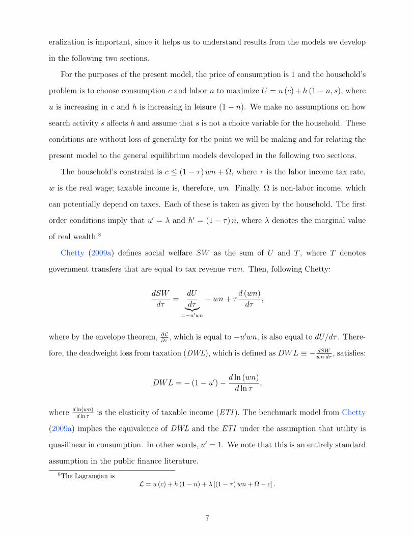
Chetty (2009a) defines social welfare SW as the sum of U and T , where T denotes

government transfers that are equal to tax revenue τwn. Then, following Chetty:

dSW

dτ=

dU

dτ︸︷︷︸=−u′wn

+ wn+ τd (wn)

dτ,

where by the envelope theorem, ∂L∂τ

, which is equal to −u′wn, is also equal to dU/dτ . There-

fore, the deadweight loss from taxation (DWL), which is defined as DWL ≡ − dSWwn·dτ , satisfies:

DWL = − (1− u′)− d ln (wn)

d ln τ,

where d ln(wn)d ln τ

is the elasticity of taxable income (ETI ). The benchmark model from Chetty

(2009a) implies the equivalence of DWL and the ETI under the assumption that utility is

quasilinear in consumption. In other words, u′ = 1. We note that this is an entirely standard

assumption in the public finance literature.

8The Lagrangian isL = u (c) + h (1− n) + λ [(1− τ)wn+ Ω− c] .

7

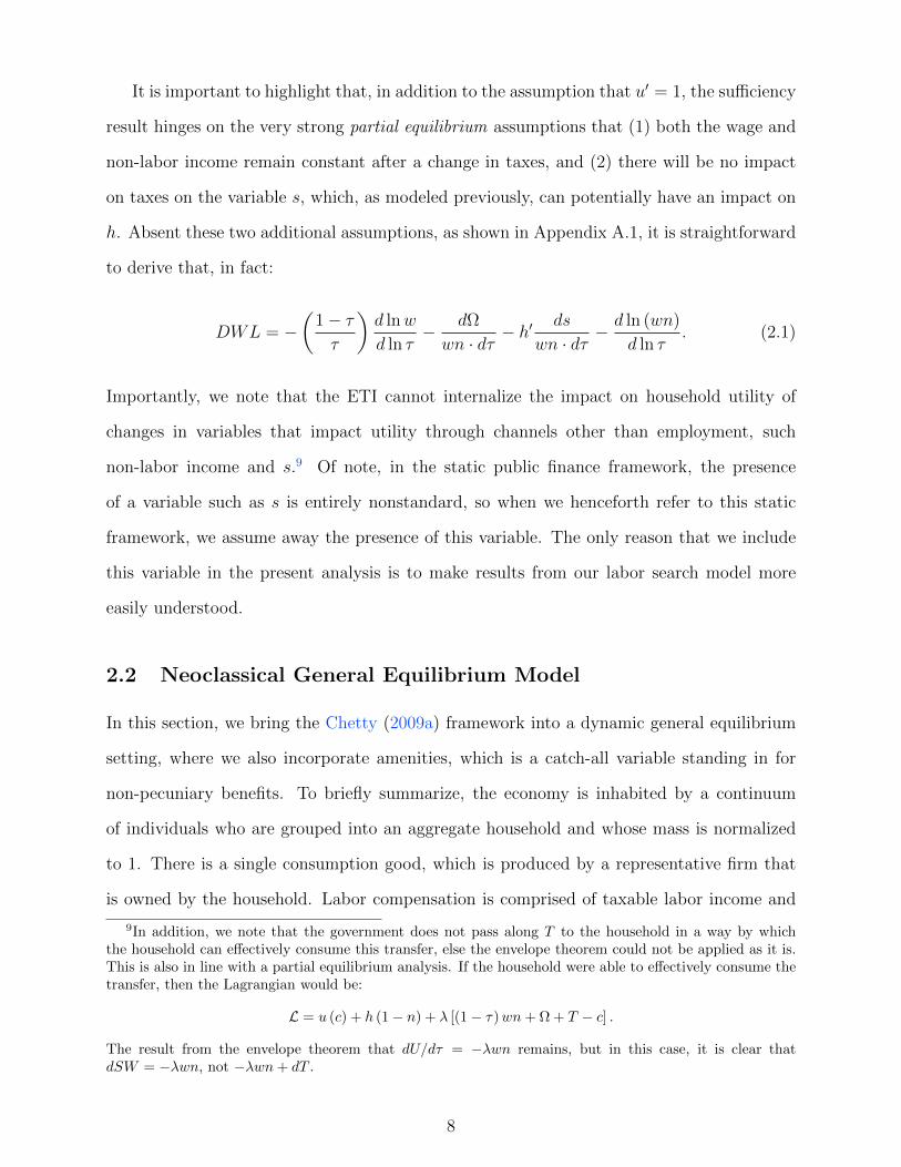
It is important to highlight that, in addition to the assumption that u′ = 1, the sufficiency

result hinges on the very strong partial equilibrium assumptions that (1) both the wage and

non-labor income remain constant after a change in taxes, and (2) there will be no impact

on taxes on the variable s, which, as modeled previously, can potentially have an impact on

h. Absent these two additional assumptions, as shown in Appendix A.1, it is straightforward

to derive that, in fact:

DWL = −(

1− ττ

)d lnw

d ln τ− dΩ

wn · dτ− h′ ds

wn · dτ− d ln (wn)

d ln τ. (2.1)

Importantly, we note that the ETI cannot internalize the impact on household utility of

changes in variables that impact utility through channels other than employment, such

non-labor income and s.9 Of note, in the static public finance framework, the presence

of a variable such as s is entirely nonstandard, so when we henceforth refer to this static

framework, we assume away the presence of this variable. The only reason that we include

this variable in the present analysis is to make results from our labor search model more

easily understood.

2.2 Neoclassical General Equilibrium Model

In this section, we bring the Chetty (2009a) framework into a dynamic general equilibrium

setting, where we also incorporate amenities, which is a catch-all variable standing in for

non-pecuniary benefits. To briefly summarize, the economy is inhabited by a continuum

of individuals who are grouped into an aggregate household and whose mass is normalized

to 1. There is a single consumption good, which is produced by a representative firm that

is owned by the household. Labor compensation is comprised of taxable labor income and

9In addition, we note that the government does not pass along T to the household in a way by whichthe household can effectively consume this transfer, else the envelope theorem could not be applied as it is.This is also in line with a partial equilibrium analysis. If the household were able to effectively consume thetransfer, then the Lagrangian would be:

L = u (c) + h (1− n) + λ [(1− τ)wn+ Ω + T − c] .

The result from the envelope theorem that dU/dτ = −λwn remains, but in this case, it is clear thatdSW = −λwn, not −λwn+ dT .

8

(non-pecuniary) amenities, and the household obtains utility from consumption, leisure, and

amenities. Amenities are produced by the firm at a cost. Finally, all markets are perfectly

competitive, and in this first pass at the general equilibrium neoclassical model and for the

purposes of generality, we assume that production takes as inputs both capital and labor.

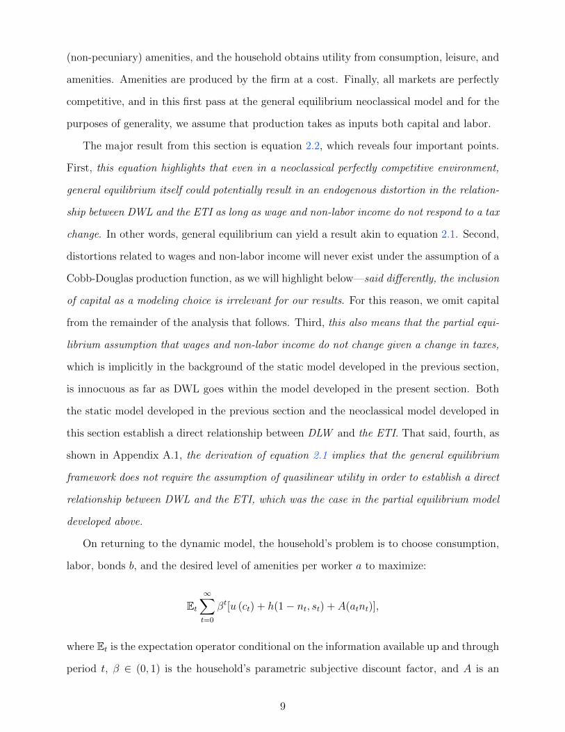
The major result from this section is equation 2.2, which reveals four important points.

First, this equation highlights that even in a neoclassical perfectly competitive environment,

general equilibrium itself could potentially result in an endogenous distortion in the relation-

ship between DWL and the ETI as long as wage and non-labor income do not respond to a tax

change. In other words, general equilibrium can yield a result akin to equation 2.1. Second,

distortions related to wages and non-labor income will never exist under the assumption of a

Cobb-Douglas production function, as we will highlight below—said differently, the inclusion

of capital as a modeling choice is irrelevant for our results. For this reason, we omit capital

from the remainder of the analysis that follows. Third, this also means that the partial equi-

librium assumption that wages and non-labor income do not change given a change in taxes,

which is implicitly in the background of the static model developed in the previous section,

is innocuous as far as DWL goes within the model developed in the present section. Both

the static model developed in the previous section and the neoclassical model developed in

this section establish a direct relationship between DLW and the ETI. That said, fourth, as

shown in Appendix A.1, the derivation of equation 2.1 implies that the general equilibrium

framework does not require the assumption of quasilinear utility in order to establish a direct

relationship between DWL and the ETI, which was the case in the partial equilibrium model

developed above.

On returning to the dynamic model, the household’s problem is to choose consumption,

labor, bonds b, and the desired level of amenities per worker a to maximize:

Et∞∑t=0

βt[u (ct) + h(1− nt, st) + A(atnt)],

where Et is the expectation operator conditional on the information available up and through

period t, β ∈ (0, 1) is the household’s parametric subjective discount factor, and A is an

9

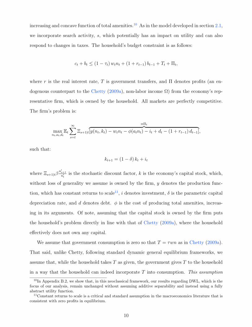
increasing and concave function of total amenities.10 As in the model developed in section 2.1,

we incorporate search activity, s, which potentially has an impact on utility and can also

respond to changes in taxes. The household’s budget constraint is as follows:

ct + bt ≤ (1− τt)wtnt + (1 + rt−1) bt−1 + Tt + Πt,

where r is the real interest rate, T is government transfers, and Π denotes profits (an en-

dogenous counterpart to the Chetty (2009a), non-labor income Ω) from the economy’s rep-

resentative firm, which is owned by the household. All markets are perfectly competitive.

The firm’s problem is:

maxnt,at,dt

Et∞∑s=t

Ξs+1|t

≡Πt︷︸︸︷[y(nt, kt)− wtnt − φ(atnt)− it + dt − (1 + rt−1) dt−1],

such that:

kt+1 = (1− δ) kt + it

where Ξs+1|tβu′s+1

u′tis the stochastic discount factor, k is the economy’s capital stock, which,

without loss of generality we assume is owned by the firm, y denotes the production func-

tion, which has constant returns to scale11, i denotes investment, δ is the parametric capital

depreciation rate, and d denotes debt. φ is the cost of producing total amenities, increas-

ing in its arguments. Of note, assuming that the capital stock is owned by the firm puts

the household’s problem directly in line with that of Chetty (2009a), where the household

effectively does not own any capital.

We assume that government consumption is zero so that T = τwn as in Chetty (2009a).

That said, unlike Chetty, following standard dynamic general equilibrium frameworks, we

assume that, while the household takes T as given, the government gives T to the household

in a way that the household can indeed incorporate T into consumption. This assumption

10In Appendix B.2, we show that, in this neoclassical framework, our results regarding DWL, which is thefocus of our analysis, remain unchanged without assuming additive separability and instead using a fullyabstract utility function.

11Constant returns to scale is a critical and standard assumption in the macroeconomics literature that isconsistent with zero profits in equilibrium.

10

does not have any first-order impact on our results—indeed, as shown in Appendix A.2, if in

the Chetty (2009a) framework we assume that T is indeed consumed by the household, then

assuming that u′ = 1 DWL is exactly the same as in equation 2.1.

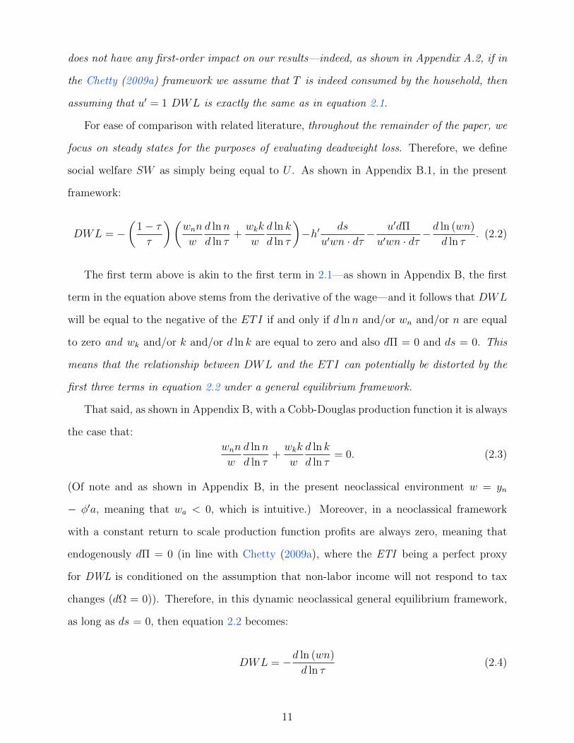
For ease of comparison with related literature, throughout the remainder of the paper, we

focus on steady states for the purposes of evaluating deadweight loss. Therefore, we define

social welfare SW as simply being equal to U . As shown in Appendix B.1, in the present

framework:

DWL = −(

1− ττ

)(wnn

w

d lnn

d ln τ+wkk

w

d ln k

d ln τ

)−h′ ds

u′wn · dτ− u′dΠ

u′wn · dτ− d ln (wn)

d ln τ. (2.2)

The first term above is akin to the first term in 2.1—as shown in Appendix B, the first

term in the equation above stems from the derivative of the wage—and it follows that DWL

will be equal to the negative of the ETI if and only if d lnn and/or wn and/or n are equal

to zero and wk and/or k and/or d ln k are equal to zero and also dΠ = 0 and ds = 0. This

means that the relationship between DWL and the ETI can potentially be distorted by the

first three terms in equation 2.2 under a general equilibrium framework.

That said, as shown in Appendix B, with a Cobb-Douglas production function it is always

the case that:

wnn

w

d lnn

d ln τ+wkk

w

d ln k

d ln τ= 0. (2.3)

(Of note and as shown in Appendix B, in the present neoclassical environment w = yn

− φ′a, meaning that wa < 0, which is intuitive.) Moreover, in a neoclassical framework

with a constant return to scale production function profits are always zero, meaning that

endogenously dΠ = 0 (in line with Chetty (2009a), where the ETI being a perfect proxy

for DWL is conditioned on the assumption that non-labor income will not respond to tax

changes (dΩ = 0)). Therefore, in this dynamic neoclassical general equilibrium framework,

as long as ds = 0, then equation 2.2 becomes:

DWL = −d ln (wn)

d ln τ(2.4)

11

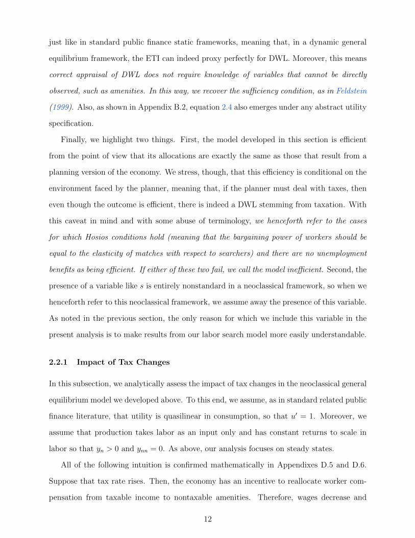
just like in standard public finance static frameworks, meaning that, in a dynamic general

equilibrium framework, the ETI can indeed proxy perfectly for DWL. Moreover, this means

correct appraisal of DWL does not require knowledge of variables that cannot be directly

observed, such as amenities. In this way, we recover the sufficiency condition, as in Feldstein

(1999). Also, as shown in Appendix B.2, equation 2.4 also emerges under any abstract utility

specification.

Finally, we highlight two things. First, the model developed in this section is efficient

from the point of view that its allocations are exactly the same as those that result from a

planning version of the economy. We stress, though, that this efficiency is conditional on the

environment faced by the planner, meaning that, if the planner must deal with taxes, then

even though the outcome is efficient, there is indeed a DWL stemming from taxation. With

this caveat in mind and with some abuse of terminology, we henceforth refer to the cases

for which Hosios conditions hold (meaning that the bargaining power of workers should be

equal to the elasticity of matches with respect to searchers) and there are no unemployment

benefits as being efficient. If either of these two fail, we call the model inefficient. Second, the

presence of a variable like s is entirely nonstandard in a neoclassical framework, so when we

henceforth refer to this neoclassical framework, we assume away the presence of this variable.

As noted in the previous section, the only reason for which we include this variable in the

present analysis is to make results from our labor search model more easily understandable.

2.2.1 Impact of Tax Changes

In this subsection, we analytically assess the impact of tax changes in the neoclassical general

equilibrium model we developed above. To this end, we assume, as in standard related public

finance literature, that utility is quasilinear in consumption, so that u′ = 1. Moreover, we

assume that production takes labor as an input only and has constant returns to scale in

labor so that yn > 0 and ynn = 0. As above, our analysis focuses on steady states.

All of the following intuition is confirmed mathematically in Appendixes D.5 and D.6.

Suppose that tax rate rises. Then, the economy has an incentive to reallocate worker com-

pensation from taxable income to nontaxable amenities. Therefore, wages decrease and

12

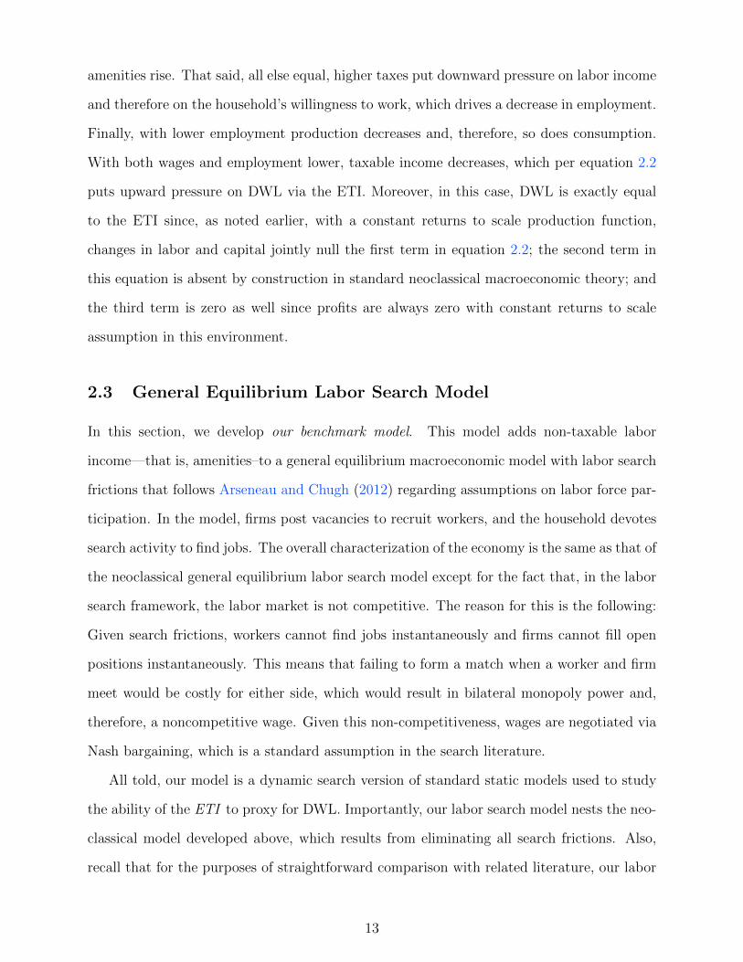
amenities rise. That said, all else equal, higher taxes put downward pressure on labor income

and therefore on the household’s willingness to work, which drives a decrease in employment.

Finally, with lower employment production decreases and, therefore, so does consumption.

With both wages and employment lower, taxable income decreases, which per equation 2.2

puts upward pressure on DWL via the ETI. Moreover, in this case, DWL is exactly equal

to the ETI since, as noted earlier, with a constant returns to scale production function,

changes in labor and capital jointly null the first term in equation 2.2; the second term in

this equation is absent by construction in standard neoclassical macroeconomic theory; and

the third term is zero as well since profits are always zero with constant returns to scale

assumption in this environment.

2.3 General Equilibrium Labor Search Model

In this section, we develop our benchmark model. This model adds non-taxable labor

income—that is, amenities–to a general equilibrium macroeconomic model with labor search

frictions that follows Arseneau and Chugh (2012) regarding assumptions on labor force par-

ticipation. In the model, firms post vacancies to recruit workers, and the household devotes

search activity to find jobs. The overall characterization of the economy is the same as that of

the neoclassical general equilibrium labor search model except for the fact that, in the labor

search framework, the labor market is not competitive. The reason for this is the following:

Given search frictions, workers cannot find jobs instantaneously and firms cannot fill open

positions instantaneously. This means that failing to form a match when a worker and firm

meet would be costly for either side, which would result in bilateral monopoly power and,

therefore, a noncompetitive wage. Given this non-competitiveness, wages are negotiated via

Nash bargaining, which is a standard assumption in the search literature.

All told, our model is a dynamic search version of standard static models used to study

the ability of the ETI to proxy for DWL. Importantly, our labor search model nests the neo-

classical model developed above, which results from eliminating all search frictions. Also,

recall that for the purposes of straightforward comparison with related literature, our labor

13

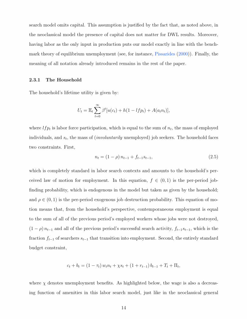
search model omits capital. This assumption is justified by the fact that, as noted above, in

the neoclassical model the presence of capital does not matter for DWL results. Moreover,

having labor as the only input in production puts our model exactly in line with the bench-

mark theory of equilibrium unemployment (see, for instance, Pissarides (2000)). Finally, the

meaning of all notation already introduced remains in the rest of the paper.

2.3.1 The Household

The household’s lifetime utility is given by:

Ut = Et∞∑t=0

βt[u(ct) + h(1− lfpt) + A(atnt)],

where lfpt is labor force participation, which is equal to the sum of nt, the mass of employed

individuals, and st, the mass of (involuntarily unemployed) job seekers. The household faces

two constraints. First,

nt = (1− ρ)nt−1 + ft−1st−1, (2.5)

which is completely standard in labor search contexts and amounts to the household’s per-

ceived law of motion for employment. In this equation, f ∈ (0, 1) is the per-period job-

finding probability, which is endogenous in the model but taken as given by the household;

and ρ ∈ (0, 1) is the per-period exogenous job destruction probability. This equation of mo-

tion means that, from the household’s perspective, contemporaneous employment is equal

to the sum of all of the previous period’s employed workers whose jobs were not destroyed,

(1− ρ)nt−1 and all of the previous period’s successful search activity, ft−1st−1, which is the

fraction ft−1 of searchers st−1 that transition into employment. Second, the entirely standard

budget constraint,

ct + bt = (1− τt)wtnt + χst + (1 + rt−1) bt−1 + Tt + Πt,

where χ denotes unemployment benefits. As highlighted below, the wage is also a decreas-

ing function of amenities in this labor search model, just like in the neoclassical general

14

equilibrium model.

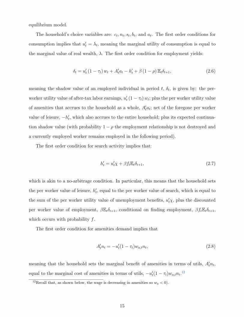
The household’s choice variables are: ct, nt, st, bt, and at. The first order conditions for

consumption implies that u′t = λt, meaning the marginal utility of consumption is equal to

the marginal value of real wealth, λ. The first order condition for employment yields:

δt = u′t (1− τt)wt + A′tat − h′t + β (1− ρ)Etδt+1, (2.6)

meaning the shadow value of an employed individual in period t, δt, is given by: the per-

worker utility value of after-tax labor earnings, u′t (1− τt)wt; plus the per worker utility value

of amenities that accrues to the household as a whole, A′tat; net of the foregone per worker

value of leisure, −h′t, which also accrues to the entire household; plus its expected continua-

tion shadow value (with probability 1− ρ the employment relationship is not destroyed and

a currently employed worker remains employed in the following period).

The first order condition for search activity implies that:

h′t = u′tχ+ βftEtδt+1, (2.7)

which is akin to a no-arbitrage condition. In particular, this means that the household sets

the per worker value of leisure, h′t, equal to the per worker value of search, which is equal to

the sum of the per worker utility value of unemployment benefits, u′tχ, plus the discounted

per worker value of employment, βEtδt+1, conditional on finding employment, βftEtδt+1,

which occurs with probability f .

The first order condition for amenities demand implies that

A′tnt = −u′t(1− τt)wa,tnt, (2.8)

meaning that the household sets the marginal benefit of amenities in terms of utils, A′tnt,

equal to the marginal cost of amenities in terms of utils, −u′t(1− τt)wa,tnt.12

12Recall that, as shown below, the wage is decreasing in amenities so wa < 0).

15

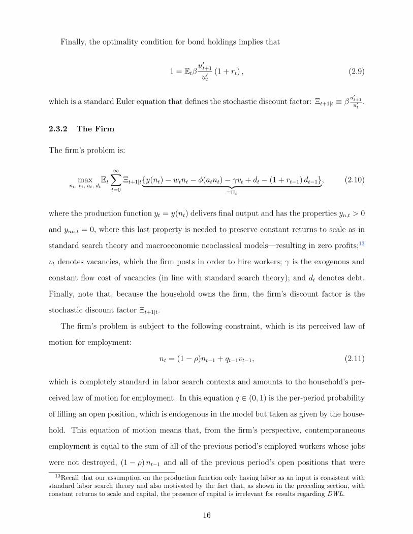
Finally, the optimality condition for bond holdings implies that

1 = Etβu′t+1

u′t(1 + rt) , (2.9)

which is a standard Euler equation that defines the stochastic discount factor: Ξt+1|t ≡ βu′t+1

u′t.

2.3.2 The Firm

The firm’s problem is:

maxnt, vt, at, dt

Et∞∑t=0

Ξt+1|ty(nt)− wtnt − φ(atnt)− γvt + dt − (1 + rt−1) dt−1︸︷︷︸≡Πt

, (2.10)

where the production function yt = y(nt) delivers final output and has the properties yn,t > 0

and ynn,t = 0, where this last property is needed to preserve constant returns to scale as in

standard search theory and macroeconomic neoclassical models—resulting in zero profits;13

vt denotes vacancies, which the firm posts in order to hire workers; γ is the exogenous and

constant flow cost of vacancies (in line with standard search theory); and dt denotes debt.

Finally, note that, because the household owns the firm, the firm’s discount factor is the

stochastic discount factor Ξt+1|t.

The firm’s problem is subject to the following constraint, which is its perceived law of

motion for employment:

nt = (1− ρ)nt−1 + qt−1vt−1, (2.11)

which is completely standard in labor search contexts and amounts to the household’s per-

ceived law of motion for employment. In this equation q ∈ (0, 1) is the per-period probability

of filling an open position, which is endogenous in the model but taken as given by the house-

hold. This equation of motion means that, from the firm’s perspective, contemporaneous

employment is equal to the sum of all of the previous period’s employed workers whose jobs

were not destroyed, (1− ρ)nt−1 and all of the previous period’s open positions that were

13Recall that our assumption on the production function only having labor as an input is consistent withstandard labor search theory and also motivated by the fact that, as shown in the preceding section, withconstant returns to scale and capital, the presence of capital is irrelevant for results regarding DWL.

16

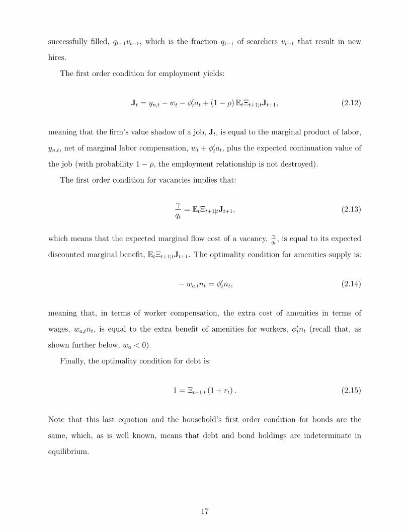
successfully filled, qt−1vt−1, which is the fraction qt−1 of searchers vt−1 that result in new

hires.

The first order condition for employment yields:

Jt = yn,t − wt − φ′tat + (1− ρ)EtΞt+1|tJt+1, (2.12)

meaning that the firm’s value shadow of a job, Jt, is equal to the marginal product of labor,

yn,t, net of marginal labor compensation, wt + φ′tat, plus the expected continuation value of

the job (with probability 1− ρ, the employment relationship is not destroyed).

The first order condition for vacancies implies that:

γ

qt= EtΞt+1|tJt+1, (2.13)

which means that the expected marginal flow cost of a vacancy, γqt

, is equal to its expected

discounted marginal benefit, EtΞt+1|tJt+1. The optimality condition for amenities supply is:

− wa,tnt = φ′tnt, (2.14)

meaning that, in terms of worker compensation, the extra cost of amenities in terms of

wages, wa,tnt, is equal to the extra benefit of amenities for workers, φ′tnt (recall that, as

shown further below, wa < 0).

Finally, the optimality condition for debt is:

1 = Ξt+1|t (1 + rt) . (2.15)

Note that this last equation and the household’s first order condition for bonds are the

same, which, as is well known, means that debt and bond holdings are indeterminate in

equilibrium.

17

2.3.3 Closing the Model

We assume that government consumption is zero so that the sum of lump sum transfers to

households and unemployment benefits equal total tax revenue:

Tt + χst = τtwtnt. (2.16)

Therefore, the aggregate resource constraint is given by

yt = ct + γvt + φ. (2.17)

Total matches in any given period, mt are increasing and concave in vacancies and

searchers in line with standard search theory. This implies that the job-finding probability

satisfies ft = mt/st and is increasing in the ratio of vacancies to searchers, vt/st (intuitively,

the more vacancies per searcher there are, the easier it is for searchers to find jobs), and that

the job-filling probability satisfies qt = mt/vt and is decreasing in the ratio of vt/st (intu-

itively, the more searchers there are, the easier it is for firms to fill open position). Moreover,

as in standard search theory, θt ≡ vt/st is market tightness. The higher this ratio is, the

easier it is for workers to find jobs.

We pause here a moment to highlight the following. The fact that f ′ (v/s) > 0 and

q′ (v/s) < 0 highlights the labor search theory congestion externality. This externality reflects

the fact that an additional searcher decreases the probability of all searchers finding a job,

and an additional vacancy decreases the probability of all vacancies being filled. Since the

firm and household take, q and f as given, respectively, then the firm and household do not

internalize the labor market impact of additional vacancies and search activity. In addition,

we note that there are “thick market externalities.” This refers to the impact of firm actions

on searchers and the impact of searcher actions on firms, which are not internalized by either

party. In particular, if search activity rises, then two countervailing outcomes are at play:

(1) congestion externalities increase for workers, and (2) thick market externalities decrease

for firms because the probability of firms filling positions rises with higher search activity.

18

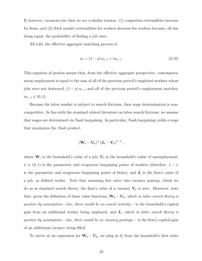
If, however, vacancies rise then we see a similar tension: (1) congestion externalities increase

for firms, and (2) thick market externalities for workers decrease for workers because, all else

being equal, the probability of finding a job rises.

All told, the effective aggregate matching process is:

nt = (1− ρ)nt−1 +mt−1. (2.18)

This equation of motion means that, from the effective aggregate perspective, contempora-

neous employment is equal to the sum of all of the previous period’s employed workers whose

jobs were not destroyed, (1− ρ)nt−1 and all of the previous period’s employment matches,

mt−1 ∈ (0, 1).

Because the labor market is subject to search frictions, then wage determination is non-

competitive. In line with the standard related literature on labor search frictions, we assume

that wages are determined via Nash bargaining. In particular, Nash bargaining yields a wage

that maximizes the Nash product,

(Wt −Ut)ψ (Jt −Vt)

1−ψ ,

where Wt is the household’s value of a job; Ut is the household’s value of unemployment;

ψ ∈ (0, 1) is the parametric and exogenous bargaining power of workers (therefore, 1 − ψ

is the parametric and exogenous bargaining power of firms); and Jt is the firm’s value of

a job, as defined earlier. Note that assuming free entry into vacancy posting, which we

do as in standard search theory, the firm’s value of a vacancy Vt is zero. Moreover, note

that, given the definition of these value functions, Wt −Ut, which in labor search theory is

positive by assumption—else, there would be no search activity— is the household’s capital

gain from an additional worker being employed, and Jt, which in labor search theory is

positive by assumption—else, there would be no vacancy postings— is the firm’s capital gain

of an additional vacancy being filled.

To arrive at an expression for Wt −Ut, we plug in h′t from the household’s first order

19

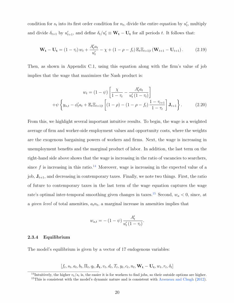
condition for st into its first order condition for nt, divide the entire equation by u′t, multiply

and divide δt+1 by u′t+1, and define δt/u′t ≡Wt −Ut for all periods t. It follows that:

Wt −Ut = (1− τt)wt +A′tatu′t− χ+ (1− ρ− ft)EtΞt+1|t (Wt+1 −Ut+1) . (2.19)

Then, as shown in Appendix C.1, using this equation along with the firm’s value of job

implies that the wage that maximizes the Nash product is:

wt = (1− ψ)

[χ

1− τt− A′tatu′t (1− τt)

]+ψ

yn,t − φ′tat + EtΞt+1|t

[(1− ρ)− (1− ρ− ft)

1− τt+1

1− τt

]Jt+1

. (2.20)

From this, we highlight several important intuitive results. To begin, the wage is a weighted

average of firm and worker-side employment values and opportunity costs, where the weights

are the exogenous bargaining powers of workers and firms. Next, the wage is increasing in

unemployment benefits and the marginal product of labor. In addition, the last term on the

right-hand side above shows that the wage is increasing in the ratio of vacancies to searchers,

since f is increasing in this ratio.14 Moreover, wage is increasing in the expected value of a

job, Jt+1, and decreasing in contemporary taxes. Finally, we note two things. First, the ratio

of future to contemporary taxes in the last term of the wage equation captures the wage

rate’s optimal inter-temporal smoothing given changes in taxes.15 Second, wa < 0, since, at

a given level of total amenities, atnt, a marginal increase in amenities implies that

wa,t = − (1− ψ)A′t

u′t (1− τt).

2.3.4 Equilibrium

The model’s equilibrium is given by a vector of 17 endogenous variables:

[ft, st, at, bt,Πt, qt,Jt, vt, dt, Tt, yt, ct, nt,Wt −Ut, wt, rt, δt]

14Intuitively, the higher vt/st is, the easier it is for workers to find jobs, so their outside options are higher.15This is consistent with the model’s dynamic nature and is consistent with Arseneau and Chugh (2012).

20

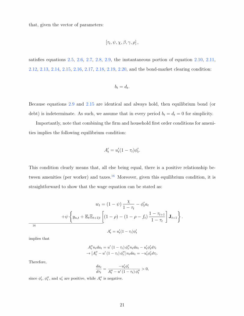
that, given the vector of parameters:

[τt, ψ, χ, β, γ, ρ] ,

satisfies equations 2.5, 2.6, 2.7, 2.8, 2.9, the instantaneous portion of equation 2.10, 2.11,

2.12, 2.13, 2.14, 2.15, 2.16, 2.17, 2.18, 2.19, 2.20, and the bond-market clearing condition:

bt = dt.

Because equations 2.9 and 2.15 are identical and always hold, then equilibrium bond (or

debt) is indeterminate. As such, we assume that in every period bt = dt = 0 for simplicity.

Importantly, note that combining the firm and household first order conditions for ameni-

ties implies the following equilibrium condition:

A′t = u′t(1− τt)φ′t.

This condition clearly means that, all else being equal, there is a positive relationship be-

tween amenities (per worker) and taxes.16 Moreover, given this equilibrium condition, it is

straightforward to show that the wage equation can be stated as:

wt = (1− ψ)χ

1− τt− φ′tat

+ψ

yn,t + EtΞt+1|t

[(1− ρ)− (1− ρ− ft)

1− τt+1

1− τt

]Jt+1

.

16

A′t = u′t(1− τt)φ′timplies that

A′′t ntdat = u′ (1− τt)φ′′t ntdat − u′tφ′tdτt→ [A′′t − u′ (1− τt)φ′′t ]ntdat = −u′tφ′tdτt.

Therefore,datdτt

=−u′tφ′t

A′′t − u′ (1− τt)φ′′t> 0,

since φ′t, φ′′t , and u′t are positive, while A′′t is negative.

21

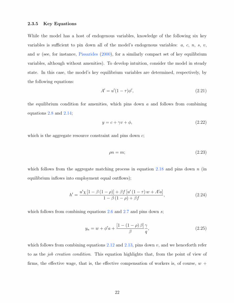
2.3.5 Key Equations

While the model has a host of endogenous variables, knowledge of the following six key

variables is sufficient to pin down all of the model’s endogenous variables: a, c, n, s, v,

and w (see, for instance, Pissarides (2000), for a similarly compact set of key equilibrium

variables, although without amenities). To develop intuition, consider the model in steady

state. In this case, the model’s key equilibrium variables are determined, respectively, by

the following equations:

A′ = u′(1− τ)φ′, (2.21)

the equilibrium condition for amenities, which pins down a and follows from combining

equations 2.8 and 2.14;

y = c+ γv + φ, (2.22)

which is the aggregate resource constraint and pins down c;

ρn = m; (2.23)

which follows from the aggregate matching process in equation 2.18 and pins down n (in

equilibrium inflows into employment equal outflows);

h′ =u′χ [1− β (1− ρ)] + βf [u′ (1− τ)w + A′a]

1− β (1− ρ) + βf, (2.24)

which follows from combining equations 2.6 and 2.7 and pins down s;

yn = w + φ′a+[1− (1− ρ) β]

β

γ

q, (2.25)

which follows from combining equations 2.12 and 2.13, pins down v, and we henceforth refer

to as the job creation condition. This equation highlights that, from the point of view of

firms, the effective wage, that is, the effective compensation of workers is, of course, w +

22

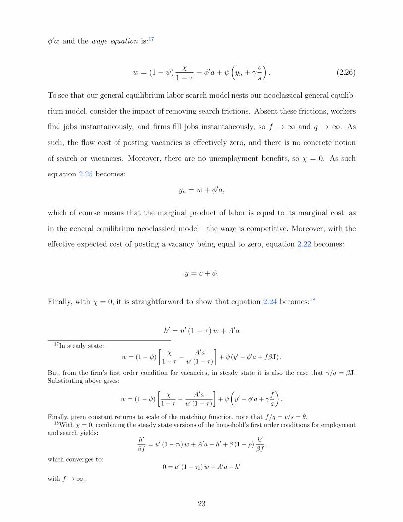
φ′a; and the wage equation is:17

w = (1− ψ)χ

1− τ− φ′a+ ψ

(yn + γ

v

s

). (2.26)

To see that our general equilibrium labor search model nests our neoclassical general equilib-

rium model, consider the impact of removing search frictions. Absent these frictions, workers

find jobs instantaneously, and firms fill jobs instantaneously, so f → ∞ and q → ∞. As

such, the flow cost of posting vacancies is effectively zero, and there is no concrete notion

of search or vacancies. Moreover, there are no unemployment benefits, so χ = 0. As such

equation 2.25 becomes:

yn = w + φ′a,

which of course means that the marginal product of labor is equal to its marginal cost, as

in the general equilibrium neoclassical model—the wage is competitive. Moreover, with the

effective expected cost of posting a vacancy being equal to zero, equation 2.22 becomes:

y = c+ φ.

Finally, with χ = 0, it is straightforward to show that equation 2.24 becomes:18

h′ = u′ (1− τ)w + A′a

17In steady state:

w = (1− ψ)

[χ

1− τ− A′a

u′ (1− τ)

]+ ψ (y′ − φ′a+ fβJ) .

But, from the firm’s first order condition for vacancies, in steady state it is also the case that γ/q = βJ.Substituting above gives:

w = (1− ψ)

[χ

1− τ− A′a

u′ (1− τ)

]+ ψ

(y′ − φ′a+ γ

f

q

).

Finally, given constant returns to scale of the matching function, note that f/q = v/s = θ.18With χ = 0, combining the steady state versions of the household’s first order conditions for employment

and search yields:h′

βf= u′ (1− τt)w +A′a− h′ + β (1− ρ)

h′

βf,

which converges to:0 = u′ (1− τt)w +A′a− h′

with f →∞.

23

and pins down employment. This, of course, is simply the general equilibrium neoclassi-

cal model’s household optimality condition for labor. All told, these last three equations,

along with equation 2.21 above, pin down the net-of-capital general equilibrium neoclassical

model’s four key variables: c, n, a, and w.

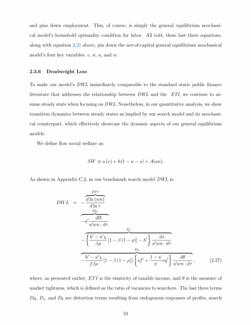
2.3.6 Deadweight Loss

To make our model’s DWL immediately comparable to the standard static public finance

literature that addresses the relationship between DWL and the ETI, we continue to as-

sume steady state when focusing on DWL. Nonetheless, in our quantitative analysis, we show

transition dynamics between steady states as implied by our search model and its neoclassi-

cal counterpart, which effectively showcase the dynamic aspects of our general equilibrium

models.

We define flow social welfare as:

SW ≡ u (c) + h(1− n− s) + A(an).

As shown in Appendix C.2, in our benchmark search model DWL is:

DWL = −

ETI︷︸︸︷d ln (wn)

d ln τDΠ︷︸︸︷

−u′ dΠ

u′wn · dτ

−

Ds︷︸︸︷h′ − u′χβρ

[1− β (1− ρ)]− h′

ds

u′wn · dτDθ︷︸︸︷

−h′ − u′χfβρ

[1− β (1− ρ)]

sf ′ +

1− ψψ

vq′

dθ

u′wn · dτ, (2.27)

where, as presented earlier, ETI is the elasticity of taxable income, and θ is the measure of

market tightness, which is defined as the ratio of vacancies to searchers. The last three terms

DΠ, Ds, and Dθ are distortion terms resulting from endogenous responses of profits, search

24

activity, and market tightness, respectively, to a tax rate change. Note that if the distortion

terms were zero, then equation 2.27 would be exactly the same as equation 2.4, meaning

that just like in the partial equilibrium public finance literature and general equilibrium

neoclassical models developed earlier, the ETI would be a perfect proxy for DWL in the

search framework.

That said, to the extent that the three distortion terms above are not all equal to zero,

then labor search introduces important distortions to the relationship between DLW and

the ETI. Clearly, all of these distortions stem from search frictions, as they owe to: changes

in search activity, which, as noted earlier, is irrelevant in a neoclassical model; changes in

profits, which are trivially zero in a neoclassical model, since profits themselves are zero in

a neoclassical model; and changes in market tightness, which as noted earlier, is irrelevant

as well in a neoclassical model. In light of the empirical importance of search frictions for

the behavior of labor markets, equation 2.27 suggests that much caution must be used when

trying to infer DWL from ETI in the presence of search frictions.

Moreover, note that the ds and dΠ terms that appear endogenously in equation 2.27

are the counterparts of the ds and dΩ or dΠ terms that had appeared in the previous two

models we developed. And, as highlighted when assessing these two models, the ETI cannot

internalize changes in social welfare that stem from non-labor income and factors other than

employment that affect the utility of households as related to labor market activity. This

result adds to the partial equilibrium evidence documenting deviations from the sufficiency

result of Feldstein (1999) driven by externalities (Chetty, 2009a; Doerrenberg et al., 2017).

In equation 2.27, the coefficient on dΠ is clearly positive, and, as shown in Appendix C.2,

the condition for the coefficient on ds being positive is δf(1−β)u′ρ

> χ, which of course holds

trivially when χ = 0. Therefore, for a given increase in taxes: if profits decrease, then this

change puts upward pressure on DWL as it means that, all else being equal, the household’s

consumption decreases. We also show in the Appendices C.2 and D.1 that the signs of ds

and its coefficient are ambiguous when χ > 0, making the impact of second distortion term

on DWL (Ds) ambiguous as well. On the other hand, when χ = 0, both ds and its coefficient

are negative, unambiguously putting upward pressure on DWL.

25

The coefficient on dθ requires further discussion as it relates directly to inefficiencies and,

in particular, to congestion externalities. As is well known, labor search models are efficient19

if two conditions hold. First, unemployment benefits χ should be equal to zero. And second,

the bargaining power of workers ψ should be equal to the elasticity of matches with respect

to searchers (this is the Hosios condition—see Hosios (1990)). If the Hosios condition holds,

then in the decentralized economy, all congestion externalities are internalized, just as they

are in a centrally planned economy.

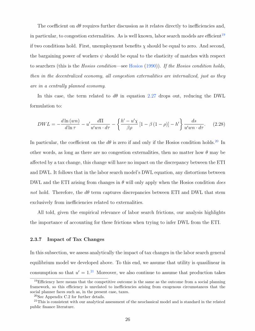
In this case, the term related to dθ in equation 2.27 drops out, reducing the DWL

formulation to:

DWL = −d ln (wn)

d ln τ− u′ dΠ

u′wn · dτ−h′ − u′χβρ

[1− β (1− ρ)]− h′

ds

u′wn · dτ. (2.28)

In particular, the coefficient on the dθ is zero if and only if the Hosios condition holds.20 In

other words, as long as there are no congestion externalities, then no matter how θ may be

affected by a tax change, this change will have no impact on the discrepancy between the ETI

and DWL. It follows that in the labor search model’s DWL equation, any distortions between

DWL and the ETI arising from changes in θ will only apply when the Hosios condition does

not hold. Therefore, the dθ term captures discrepancies between ETI and DWL that stem

exclusively from inefficiencies related to externalities.

All told, given the empirical relevance of labor search frictions, our analysis highlights

the importance of accounting for these frictions when trying to infer DWL from the ETI.

2.3.7 Impact of Tax Changes

In this subsection, we assess analytically the impact of tax changes in the labor search general

equilibrium model we developed above. To this end, we assume that utility is quasilinear in

consumption so that u′ = 1.21 Moreover, we also continue to assume that production takes

19Efficiency here means that the competitive outcome is the same as the outcome from a social planningframework, so this efficiency is unrelated to inefficiencies arising from exogenous circumstances that thesocial planner faces such as, in the present case, taxes.

20See Appendix C.2 for further details.21This is consistent with our analytical assessment of the neoclassical model and is standard in the related

public finance literature.

26

labor as an input and has constant returns to scale in labor so that yn > 0 and ynn = 0. As

above, our analysis focuses on steady states.

All of the following intuition is confirmed mathematically in Appendixes D.1 through

D.4. Suppose that taxes rise. In the efficient search framework the effective wage of the

marginal worker remains unchanged as taxable wage compensation is substituted by non-

taxable amenities.2223 As such, amenities ultimately rise and the wage decreases. In other

words, net-of-tax labor income drops because of higher taxes, and this drop results in a

decrease in search activity. With lower search activity, it becomes harder for firms to fill

jobs, so vacancies decrease, which puts downward pressure on the job finding probability.

Ultimately, these dynamics result in lower employment, which leads to lower production and

profits, both of which put downward pressure on consumption. All of these results continue

to apply in the absence of amenities too.

In the search framework with unemployment benefits, an increase in taxes puts upward

pressure on the effective wage, w + φ′a, since net-of-tax wages decline relative to non-taxed

unemployment benefits. This means that workers’ relative outside options rise for a given

increase in taxes.24 All else equal, this higher effective wage makes it more costly for firms to

produce, so vacancies ultimately drop, which is consistent with a lower job finding probability.

In terms of search incentives, there is now ambiguity. On the one hand, a higher effective

wage makes search more appealing, but on the other hand, a lower job finding probability

makes search less appealing.25 Given this ambiguity, quantitative analysis—which we turn

to in the next section—is necessary to assess which effect dominates and what ultimately

happens in this version of the model. More generally, note that, in both the cases with and

without amenities, quantitative analysis is needed to determine the ultimate effect of the

tax change on the relationship between DWL and the ETI. This is because the coefficients

in equation 2.27 have first-order impact on the extent to which changes in search activity,

22Recall, this results with no unemployment benefits χ and the Hosios condition that the bargaining powerof workers ψ being equal to the elasticity of matches with respect to searchers holds

23The effective wage is the sum of the wage and the marginal utility from amenities, w + φ′a. In the casewithout amenities, this is trivially equally to w.

24The same is true absent amenities and, again, note that absent amenities the effective wage is simplyequal to the real wage w.

25The same is true absent amenities.

27

profits, and market tightness can distort the relationship between DWL and the ETI.

3 Quantitative Analyses

In this section, we use calibrated versions of the models we developed to explore their quan-

titative implications. Importantly, recall that, in line with the literature most related to our

work, our theoretical framework is quite stylized as, for instance, it omits capital. As such,

our quantitative results should be interpreted as similarly stylized. That said, as appropri-

ate, we discuss results from six models: our benchmark labor search model with and without

amenities and, alternatively, with and without unemployment benefits, and our neoclassical

model with and without amenities.

3.1 Functional Forms

For the household, we assume a constant relative risk aversion utility function for consump-

tion, u (ct) =c1−σt

1−σ , where σ > 0 is the coefficient of relative risk aversion. This functional

form is entirely standard in the macroeconomics literature. For simplicity, as a benchmark,

we assume h (1− lfpt) = ζ ln (1− lfpt) and A (atnt) = ζa ln (atnt), where ζ > 0 and ζa > 0.

Turning to production, we assume linear production technology with yt = znt, where z is

exogenous productivity.26 We chose this functional form to preserve the constant returns

to scale property of the neoclassical model in the absence of capital. In addition, we as-

sume a general functional form for amenities production technology: in particular, let total

amenities atnt be equal to (produced by) the technology g(yatt ) = ΦyatΨt , where Φ > 0 and

Ψ > 0. Here, yatt is part of the final output allocated for amenities production. Note that

this functional form implies that the cost of total amenities is: φ(atnt) =[atnt

Φ

] 1Ψ 1

Ψ. Finally,

regarding the labor market, we assume a Cobb-Douglas matching function m = ϕvξt s1−ξt ,

where ϕ > 0 is matching efficiency and ξ ∈ (0, 1) is the elasticity of matches with respect to

vacancies. This functional form for the matching function is entirely standard in the search

26Recall that, given the irrelevance of capital for our results for the purposes of the neoclassical model, wesimply assume that output is a function of labor, so this assumption on the functional form of productionapplies to all models under consideration.

28

literature (see, for instance, Pissarides (2000), and Shimer (2005)).

3.2 Calibration

The calibration strategy described below is for the search model with amenities, though the

other variants of the model are calibrated in a similar fashion. A period is one month. This

choice is based on the fact that, given Cobb-Douglas matching functions, the probabilities f

and q are unbounded, and simulations and/or comparative static exercises frequently lead to

instances in which these probabilities exceed 1 in models calibrated at quarterly frequency. In

line with our one-month time period assumption, we set β = 0.996, which is consistent with

an average yearly interest rate of 5 percent, as is the case in the United States, on average,

in the post-war period. Continuing with the household, we choose the leisure parameter ζ so

that in equilibrium, the mass of individuals outside the labor force, 1 − lfp, is equal to 0.38.

This target is obtained using data from the Bureau of Labor Statistics (BLS) on the average

number of U.S. individuals outside of the labor force in per-population terms. We calibrate

the amenities parameter ζa by setting the amenities-to-wage ratio aw

to 0.11, following the

estimate of Hall and Mueller (2018). As a benchmark, we operationalize the model in line

with standard public finance literature by assuming utility to be quasilinear in consumption.

This assumption implies that u′ = 1, which requires setting σ = 0.

Turning to the firm, we choose the equilibrium value of exogenous productivity, z, so

that monthly output, y, equals 1. As a benchmark, we set both Ψ and Φ equal to 1, which

implies that φ (atnt) = atnt.

As related explicitly to the labor market, the wage tax τ is set to 0.189, which is the aver-

age U.S. labor tax calculated in McDaniel (2011). Moreover, implementing the methodology

from Solon et al. (2009) and Shimer (2012) and using, as they do, BLS data on unemploy-

ment and short-term unemployment, we find that the average U.S. monthly probability of

finding a job (f) in the post-war period is 0.43. The matching efficiency parameter ϕ is

chosen to hit this target. Then, ρ is chosen to set s/ (s+ n) = 0.058, which, given BLS data,

is the average U.S. unemployment rate in the post-war period.

29

Of course, the neoclassical version of the model we develop is efficient by construction. In

our benchmark calibration, our search models are also efficient in the sense that we assume

that there are no unemployment benefits, and the Hosios (1990) condition holds, meaning

that the bargaining power of workers, ψ, is set equal to the elasticity of matches with respect

to search activity, 1 − ξ. As a benchmark, we set ψ = 1 − ξ = 0.5, where the value of ξ is in

line with the empirical evidence in Pissarides and Petrongolo (2001). Moreover, we explore

the implications of efficiency as related to unemployment benefits. As such, we study the

cases with χ = 0 and χ = 0.9. The latter value is consistent with the replacement rate being

equal to 60 percent and is in line with the fact that replacement rates should target about

60 percent for the average worker under the 2015 Social Security law.

For the purposes of analysis, we recalibrate the other four models we consider where

appropriate: the search model without amenities with and without unemployment benefits

and the neoclassical model with and without amenities. However, to keep all six models

comparable, we set the levels of taxable income in each model to the level of taxable income

obtained for the calibrated benchmark search model with amenities and no unemployment

benefits instead of setting y = 1 to calibrate the productivity parameter z. As such, all

the economies we study have the same fundamentals. Table 1 summarizes our benchmark

parameter values.

As a robustness check, we calibrate all four models in the same way that we calibrated the

search model with amenities and no unemployment benefits, choosing z by setting y = 1. In

this case, the calibrated parameters are largely unchanged, leaving no visible imprint on our

quantitative findings. Hence, we do not report the results from this alternative calibration.

That said, we do present results from sensitivity analysis as related to the most critical

parameters in our calibration, and we show that our results are robust to a range of values

in these parameters. In particular, in all robustness checks, the ETI is never a perfect proxy

for the DWL and always underestimates it, though at significantly varying degrees.

30

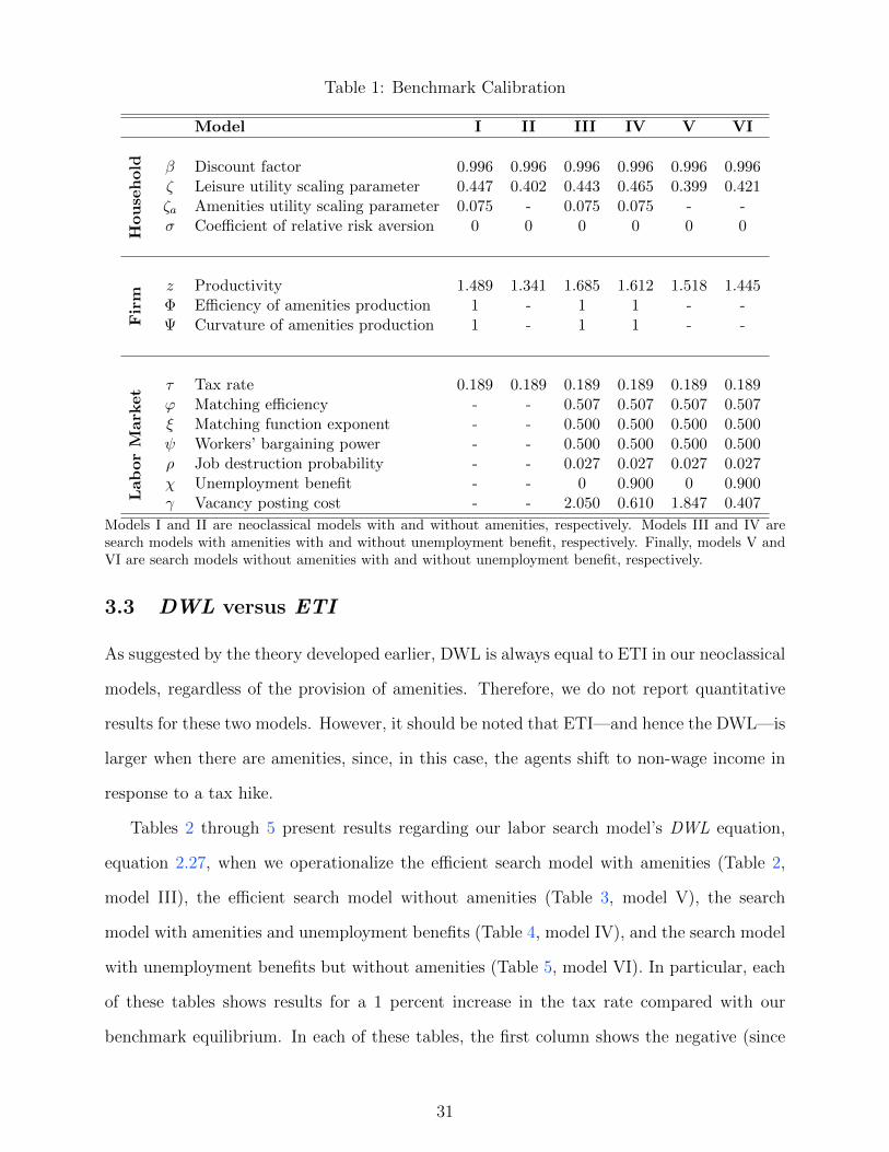
Table 1: Benchmark Calibration

Model I II III IV V VIH

ou

seh

old β Discount factor 0.996 0.996 0.996 0.996 0.996 0.996

ζ Leisure utility scaling parameter 0.447 0.402 0.443 0.465 0.399 0.421ζa Amenities utility scaling parameter 0.075 - 0.075 0.075 - -σ Coefficient of relative risk aversion 0 0 0 0 0 0

Fir

m

z Productivity 1.489 1.341 1.685 1.612 1.518 1.445Φ Efficiency of amenities production 1 - 1 1 - -Ψ Curvature of amenities production 1 - 1 1 - -

Lab

or

Mark

et τ Tax rate 0.189 0.189 0.189 0.189 0.189 0.189

ϕ Matching efficiency - - 0.507 0.507 0.507 0.507ξ Matching function exponent - - 0.500 0.500 0.500 0.500ψ Workers’ bargaining power - - 0.500 0.500 0.500 0.500ρ Job destruction probability - - 0.027 0.027 0.027 0.027χ Unemployment benefit - - 0 0.900 0 0.900γ Vacancy posting cost - - 2.050 0.610 1.847 0.407

Models I and II are neoclassical models with and without amenities, respectively. Models III and IV aresearch models with amenities with and without unemployment benefit, respectively. Finally, models V andVI are search models without amenities with and without unemployment benefit, respectively.

3.3 DWL versus ETI

As suggested by the theory developed earlier, DWL is always equal to ETI in our neoclassical

models, regardless of the provision of amenities. Therefore, we do not report quantitative

results for these two models. However, it should be noted that ETI—and hence the DWL—is

larger when there are amenities, since, in this case, the agents shift to non-wage income in

response to a tax hike.

Tables 2 through 5 present results regarding our labor search model’s DWL equation,

equation 2.27, when we operationalize the efficient search model with amenities (Table 2,

model III), the efficient search model without amenities (Table 3, model V), the search

model with amenities and unemployment benefits (Table 4, model IV), and the search model

with unemployment benefits but without amenities (Table 5, model VI). In particular, each

of these tables shows results for a 1 percent increase in the tax rate compared with our

benchmark equilibrium. In each of these tables, the first column shows the negative (since

31

that is the way in which they enter equation 2.27) of the value of the coefficients on the ETI,

dΠ/dτ , ds/dτ , and dθ/dτ (rows 1 through 4, respectively). Column 3 shows the values of

the ETI, dΠ/dτ , ds/dτ , and dθ/dτ (rows 1 through 4, respectively). Column 4 shows the

product of columns 1 and 3 (i.e., each row in column 4 corresponds to the ETI or one of

three distortion terms in equation 2.27). Finally, column 5 shows the percent of the ETI of

each value in column 4, and the last row of column 5 shows the sum of these percentages,

which corresponds to the DWL arising from the tax change. As such, these tables break

down DWL by each term on the right-hand side of equation 2.27. Note that Appendix E

complements this section by discussing the particular implications of our calibration, which

will help the reader understand the magnitudes of ETIs and distortion terms across models,

as presented in following tables.

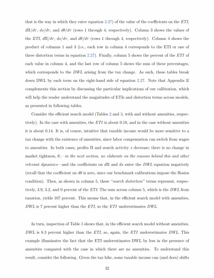
Consider the efficient search model (Tables 2 and 3, with and without amenities, respec-

tively). In the case with amenities, the ETI is about 0.18, and in the case without amenities

it is about 0.14. It is, of course, intuitive that taxable income would be more sensitive to a

tax change with the existence of amenities, since labor compensation can switch from wages

to amenities. In both cases, profits Π and search activity s decrease; there is no change in

market tightness, θ,—in the next section, we elaborate on the reasons behind this and other

relevant dynamics—and the coefficients on dΠ and ds enter the DWL equation negatively

(recall that the coefficient on dθ is zero, since our benchmark calibrations impose the Hosios

condition). Then, as shown in column 5, these “search distortion” terms represent, respec-

tively, 3.9, 3.2, and 0 percent of the ETI. The sum across column 5, which is the DWL from

taxation, yields 107 percent. This means that, in the efficient search model with amenities,

DWL is 7 percent higher than the ETI, so the ETI underestimates DWL.

In turn, inspection of Table 3 shows that, in the efficient search model without amenities,

DWL is 8.3 percent higher than the ETI, so, again, the ETI underestimates DWL. This

example illuminates the fact that the ETI underestimates DWL by less in the presence of

amenities compared with the case in which there are no amenities. To understand this

result, consider the following. Given the tax hike, some taxable income can (and does) shifts

32

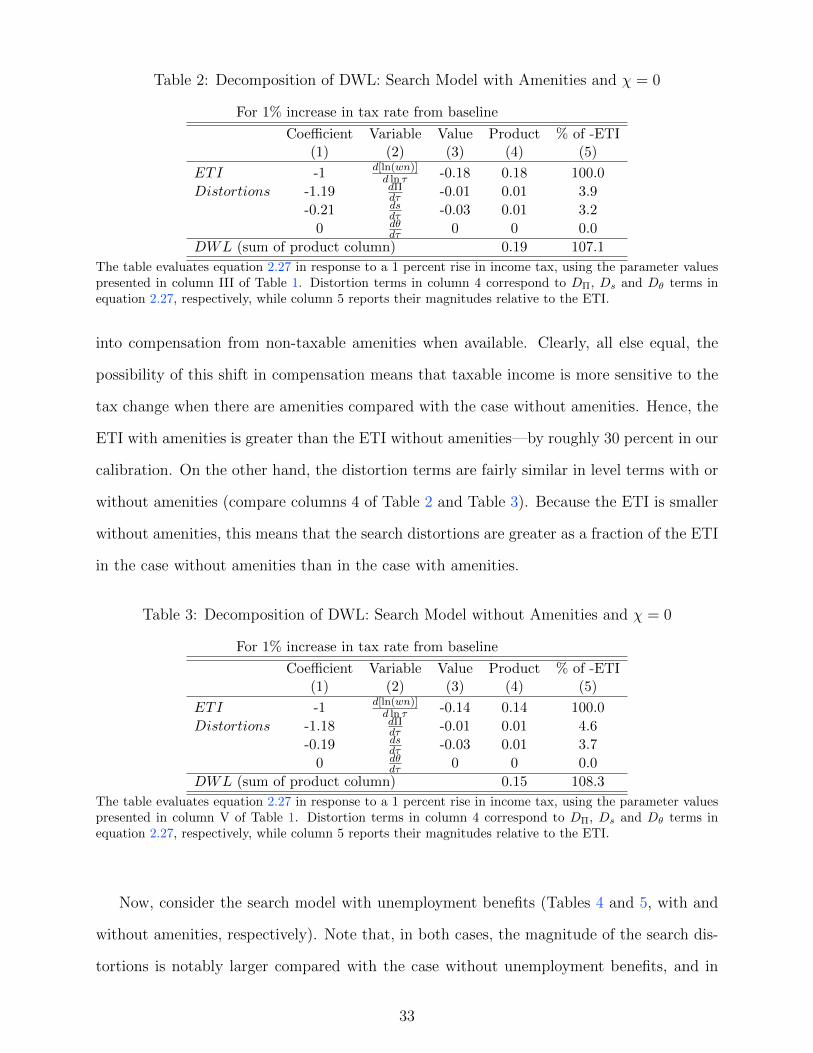
Table 2: Decomposition of DWL: Search Model with Amenities and χ = 0

For 1% increase in tax rate from baseline

Coefficient Variable Value Product % of -ETI(1) (2) (3) (4) (5)

ETI -1 d[ln(wn)]d ln τ -0.18 0.18 100.0

Distortions -1.19 dΠdτ -0.01 0.01 3.9

-0.21 dsdτ -0.03 0.01 3.2

0 dθdτ 0 0 0.0

DWL (sum of product column) 0.19 107.1

The table evaluates equation 2.27 in response to a 1 percent rise in income tax, using the parameter valuespresented in column III of Table 1. Distortion terms in column 4 correspond to DΠ, Ds and Dθ terms inequation 2.27, respectively, while column 5 reports their magnitudes relative to the ETI.

into compensation from non-taxable amenities when available. Clearly, all else equal, the

possibility of this shift in compensation means that taxable income is more sensitive to the

tax change when there are amenities compared with the case without amenities. Hence, the

ETI with amenities is greater than the ETI without amenities—by roughly 30 percent in our

calibration. On the other hand, the distortion terms are fairly similar in level terms with or

without amenities (compare columns 4 of Table 2 and Table 3). Because the ETI is smaller

without amenities, this means that the search distortions are greater as a fraction of the ETI

in the case without amenities than in the case with amenities.

Table 3: Decomposition of DWL: Search Model without Amenities and χ = 0



ETI -1 d[ln(wn)]d ln τ -0.14 0.14 100.0


-0.19 dsdτ -0.03 0.01 3.7

0 dθdτ 0 0 0.0


The table evaluates equation 2.27 in response to a 1 percent rise in income tax, using the parameter valuespresented in column V of Table 1. Distortion terms in column 4 correspond to DΠ, Ds and Dθ terms inequation 2.27, respectively, while column 5 reports their magnitudes relative to the ETI.

Now, consider the search model with unemployment benefits (Tables 4 and 5, with and

without amenities, respectively). Note that, in both cases, the magnitude of the search dis-

tortions is notably larger compared with the case without unemployment benefits, and in

33

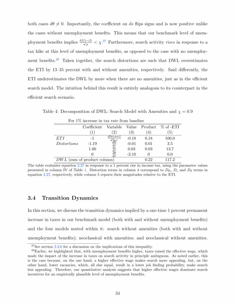
both cases dθ 6= 0. Importantly, the coefficient on ds flips signs and is now positive unlike

the cases without unemployment benefits. This means that our benchmark level of unem-

ployment benefits implies δf(1−β)u′ρ

< χ.27 Furthermore, search activity rises in response to a

tax hike at this level of unemployment benefits, as opposed to the case with no unemploy-

ment benefits.28 Taken together, the search distortions are such that DWL overestimates

the ETI by 13–35 percent with and without amenities, respectively. Said differently, the

ETI underestimates the DWL by more when there are no amenities, just as in the efficient

search model. The intuition behind this result is entirely analogous to its counterpart in the

efficient search scenario.

Table 4: Decomposition of DWL: Search Model with Amenities and χ = 0.9



ETI -1 d[ln(wn)]d ln τ -0.18 0.18 100.0


1.00 dsdτ 0.03 0.03 13.7

0 dθdτ -2.10 0 0.0


The table evaluates equation 2.27 in response to a 1 percent rise in income tax, using the parameter valuespresented in column IV of Table 1. Distortion terms in column 4 correspond to DΠ, Ds and Dθ terms inequation 2.27, respectively, while column 5 reports their magnitudes relative to the ETI.

3.4 Transition Dynamics

In this section, we discuss the transition dynamics implied by a one-time 1 percent permanent

increase in taxes in our benchmark model (both with and without unemployment benefits)

and the four models nested within it: search without amenities (both with and without

unemployment benefits); neoclassical with amenities; and neoclassical without amenities.

27See section 2.3.6 for a discussion on the implications of this inequality.28Earlier, we highlighted that, with unemployment benefits higher, taxes raised the effective wage, which

made the impact of the increase in taxes on search activity in principle ambiguous. As noted earlier, thisis the case because, on the one hand, a higher effective wage makes search more appealing, but, on theother hand, lower vacancies, which, all else equal, result in a lower job finding probability, make searchless appealing. Therefore, our quantitative analysis suggests that higher effective wages dominate searchincentives for an empirically plausible level of unemployment benefits.

34

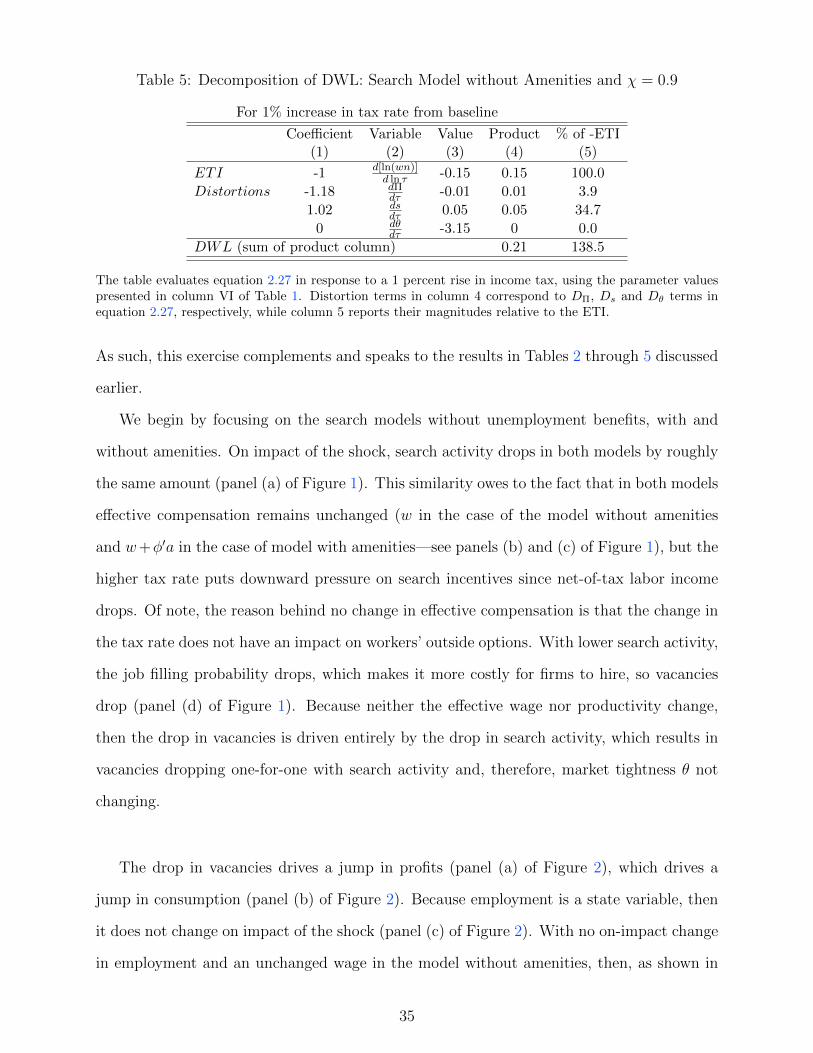
Table 5: Decomposition of DWL: Search Model without Amenities and χ = 0.9



ETI -1 d[ln(wn)]d ln τ -0.15 0.15 100.0


1.02 dsdτ 0.05 0.05 34.7

0 dθdτ -3.15 0 0.0


The table evaluates equation 2.27 in response to a 1 percent rise in income tax, using the parameter valuespresented in column VI of Table 1. Distortion terms in column 4 correspond to DΠ, Ds and Dθ terms inequation 2.27, respectively, while column 5 reports their magnitudes relative to the ETI.

As such, this exercise complements and speaks to the results in Tables 2 through 5 discussed

earlier.

We begin by focusing on the search models without unemployment benefits, with and

without amenities. On impact of the shock, search activity drops in both models by roughly

the same amount (panel (a) of Figure 1). This similarity owes to the fact that in both models

effective compensation remains unchanged (w in the case of the model without amenities

and w+φ′a in the case of model with amenities—see panels (b) and (c) of Figure 1), but the

higher tax rate puts downward pressure on search incentives since net-of-tax labor income

drops. Of note, the reason behind no change in effective compensation is that the change in

the tax rate does not have an impact on workers’ outside options. With lower search activity,

the job filling probability drops, which makes it more costly for firms to hire, so vacancies

drop (panel (d) of Figure 1). Because neither the effective wage nor productivity change,

then the drop in vacancies is driven entirely by the drop in search activity, which results in

vacancies dropping one-for-one with search activity and, therefore, market tightness θ not

changing.

The drop in vacancies drives a jump in profits (panel (a) of Figure 2), which drives a

jump in consumption (panel (b) of Figure 2). Because employment is a state variable, then

it does not change on impact of the shock (panel (c) of Figure 2). With no on-impact change

in employment and an unchanged wage in the model without amenities, then, as shown in

35

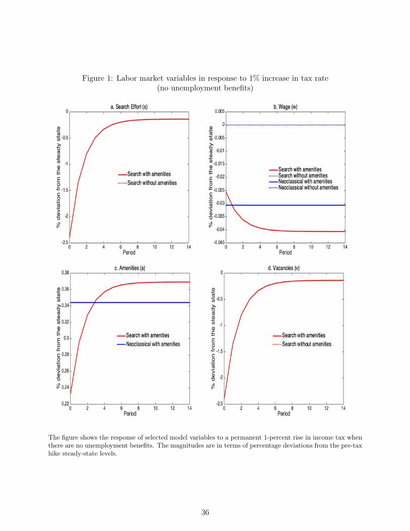
Figure 1: Labor market variables in response to 1% increase in tax rate(no unemployment benefits)

The figure shows the response of selected model variables to a permanent 1-percent rise in income tax whenthere are no unemployment benefits. The magnitudes are in terms of percentage deviations from the pre-taxhike steady-state levels.

36

panel (d) of Figure 2, taxable income in this model does not change on impact either. As

also shown in this figure, because in the model with amenities the wage indeed drops on

impact, in spite of unchanged on-impact employment, taxable income drops upon the shock.

Thereafter, lower search activity and vacancies put downward pressure on employment,

which decreases slowly and permanently. Expected lower employment implies an expected

increase in the marginal product of labor, which drives a slow-moving recovery in vacancies.

With this recovery putting upward pressure on the job finding probability, search activity

follows suit and slowly recovers as well. That said, with a permanently higher tax rate,

search activity is permanently lower as are vacancies and, therefore, employment as well.

Regarding amenities, note that, because utility from amenities and the cost of produc-

ing amenities are functions of total amenities—the product of amenities (per worker) and

employment—then amenities rise slowly, mirroring the slow-moving downward dynamic path

of employment. Of course, in terms of effective compensation, the slow-moving rise in ameni-

ties is offset by the slow-moving decline in wages as a result of the inverse relationship of

these two variables. All told, taxable income decreases slowly and permanently in both

models, owing to the slow-moving decline in employment in the model without amenities

and owing to both the slow-moving decline in employment and the slow-moving decline in

wages in the model with amenities.

With permanently lower employment, output is permanently lower as well. Given un-

changed effective wages, lower output drives profits down. Of course, in the case of the

model with amenities, in terms of profits, the decline in output outweighs the decline in

costs owing to vacancy postings. Against this backdrop, consumption declines and is ulti-

mately permanently lower given permanently lower labor income and profits. Finally, Figure

3 shows DWL and the negative of ETI for the models with and without amenities (panel (a)

and panel (b), respectively). Note that DWL is actually negative on impact of the shock,

which means that on impact of the shock there are actually welfare gains. These gains are

in line with the on-impact increase in consumption noted above29. Moreover, these gains

29This is tied to the on-impact increase in profits driven, in turn, by the on-impact decline in vacancies.

37

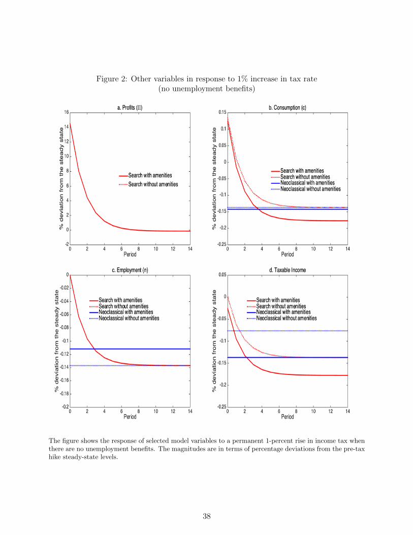
Figure 2: Other variables in response to 1% increase in tax rate(no unemployment benefits)

The figure shows the response of selected model variables to a permanent 1-percent rise in income tax whenthere are no unemployment benefits. The magnitudes are in terms of percentage deviations from the pre-taxhike steady-state levels.

38

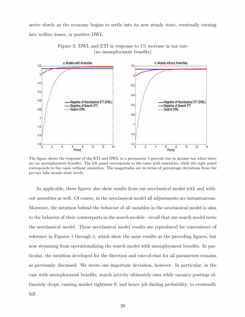
arrive slowly as the economy begins to settle into its new steady state, eventually turning

into welfare losses, or positive DWL.

Figure 3: DWL and ETI in response to 1% increase in tax rate(no unemployment benefits)

The figure shows the response of the ETI and DWL to a permanent 1-percent rise in income tax when thereare no unemployment benefits. The left panel corresponds to the cases with amenities, while the right panelcorresponds to the cases without amenities. The magnitudes are in terms of percentage deviations from thepre-tax hike steady-state levels.

As applicable, these figures also show results from our neoclassical model with and with-

out amenities as well. Of course, in the neoclassical model all adjustments are instantaneous.

Moreover, the intuition behind the behavior of all variables in the neoclassical model is akin

to the behavior of their counterparts in the search models—recall that our search model nests

the neoclassical model. These neoclassical model results are reproduced for convenience of

reference in Figures 4 through 6, which show the same results as the preceding figures, but

now stemming from operationalizing the search model with unemployment benefits. In par-

ticular, the intuition developed for the direction and rate-of-chat for all parameters remains

as previously discussed. We stress one important deviation, however. In particular, in the

case with unemployment benefits, search activity ultimately rises while vacancy postings ul-

timately drops, causing market tightness θ, and hence job finding probability, to eventually

fall.

39

3.5 Externalities

Recall that, if the Hosios condition does not hold (i.e., when the bargaining power of work-

ers is not equal to the elasticity of matches with respect to search activity— in our model’s

notation: ψ 6= 1 − ξ ), then the competitive version of search models suffers from congestion

externalities. This leads to the following two facts. First, additional searchers do not inter-

nalize that they create a greater competition for jobs by increasing the pool of searchers, and

therefore, decrease the probability of finding a job for all workers.30 Second, firms posting

additional vacancies do not internalize that they raise competition for workers by increasing

the pool of vacancies, causing the probability of filling a job to decrease for all firms. 31

While the Hosios condition is a convenient modeling assumption, there is no concrete

agreement in the search literature regarding whether or not it is empirically plausible. There-

fore, in this section, we consider the impact of relaxing the assumption that the Hosios

condition holds. Recall that, in this case, the coefficient on dθ in the search model’s DWL

equation 2.27 is no longer zero. Moreover, this coefficient is only zero if the Hosios condition

holds. As a result, changes in market tightness, θ, can be interpreted as speaking explicitly

to congestion externalities without the Hosios assumption.

Figure 7 shows results from assessing the impact of deviations from the Hosios condition

by varying the bargaining power of workers ψ while keeping the value of 1 − ξ constant.32

The left panel of this figure shows results from the search model without unemployment

benefits, and the right panel shows results with unemployment benefits. In all graphs, the

horizontal axis is ψ, which we vary between 0.4 and 0.6.33 Within these left and right panels,

at each value of ψ, the top panel shows the percentage change in search activity given a 1

percent increase in taxes; at each value of ψ, the middle panel shows the percentage change

in market tightness θ given a 1 percent increase in taxes; and at each value of ψ, the bottom

panel shows the percent difference between DWL and the ETI given a 1 percent increase in

30That said, an additional worker searching increases the probability of all firms of hiring, which is calleda thick market externality.

31That said, an additional vacancy posted increases the probability of all workers finding a job, which alsofalls into the category of a thick market externality.

32The model is recalibrated for each value of ψ.33At ψ = 0.5, which is our benchmark calibration, ψ = 1− ξ and the Hosios condition holds.

40

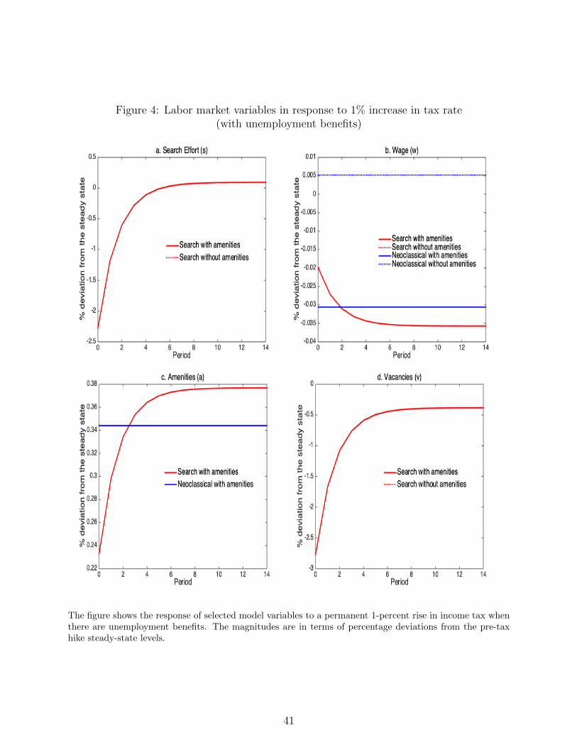
Figure 4: Labor market variables in response to 1% increase in tax rate(with unemployment benefits)

The figure shows the response of selected model variables to a permanent 1-percent rise in income tax whenthere are unemployment benefits. The magnitudes are in terms of percentage deviations from the pre-taxhike steady-state levels.

41

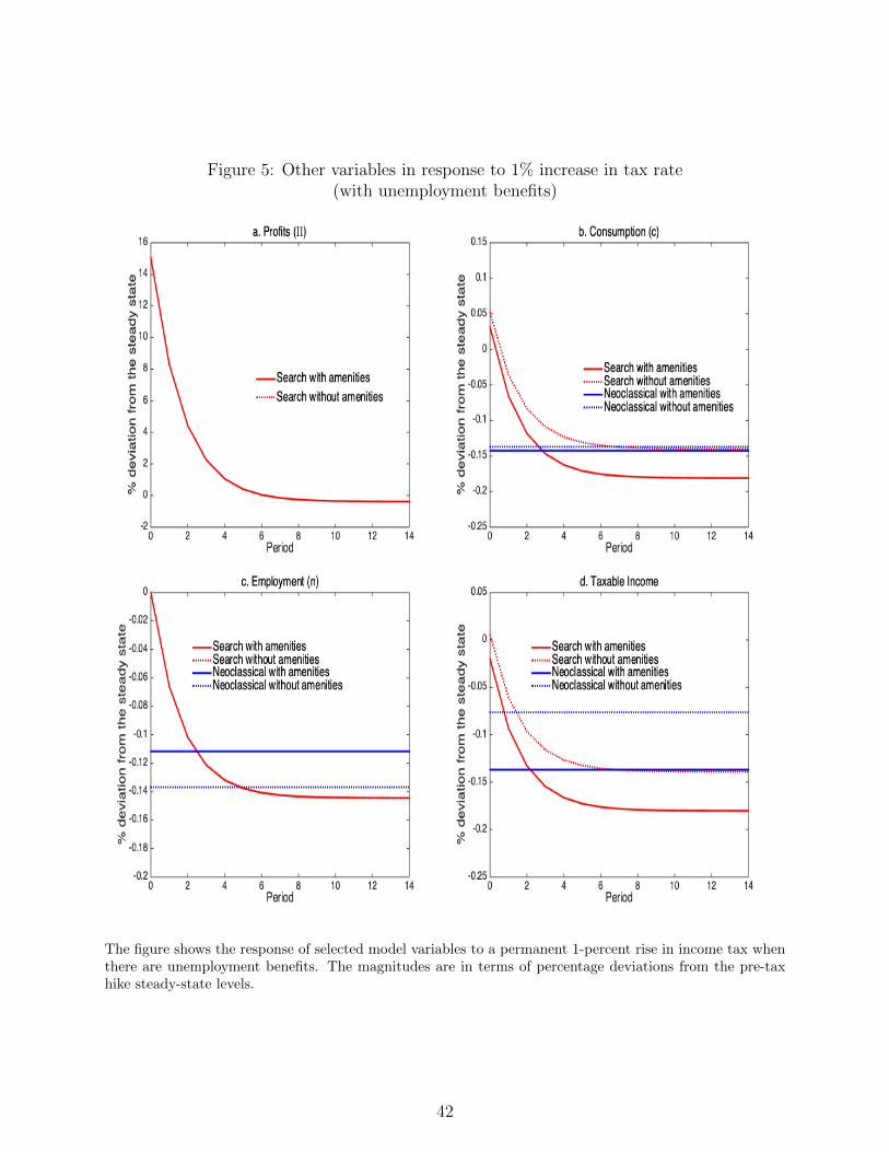
Figure 5: Other variables in response to 1% increase in tax rate(with unemployment benefits)

The figure shows the response of selected model variables to a permanent 1-percent rise in income tax whenthere are unemployment benefits. The magnitudes are in terms of percentage deviations from the pre-taxhike steady-state levels.

42

Figure 6: DWL and ETI in response to 1% increase in tax rate(with unemployment benefits)

The figure shows the response of the ETI and DWL to a permanent 1-percent rise in income tax when thereare unemployment benefits. The left panel corresponds to the cases with amenities, while the right panelcorresponds to the cases without amenities. The magnitudes are in terms of percentage deviations from thepre-tax hike steady-state levels.

taxes.

Before addressing the results, it is important to note that over the range ψ < 1−ξ = 0.5,

the coefficient on dθ is negative, and over the range ψ > 1−ξ = 0.5, it is positive.34 Moreover,

the coefficient on ds is always negative with χ = 0 and always positive with χ = 0.9, which

means that in our calibration with unemployment benefits δf(1−β)u′ρ

< χ holds. Considering

that ds > 0 when χ = 0.9, this implies that higher effective wages dominate search incentives

when there are unemployment benefits.

In Figure 7, as shown in the left panel, changes in taxes do not have an impact on market

tightness θ across ranges of ψ without unemployment benefits. This is in line with our earlier

results regarding this variable given our benchmark calibration without unemployment bene-

fits. On the other hand, throughout the range of ψ, values of search activity always decreases.

That said, in this case without unemployment benefits, as in Table 2, the effective coefficient

34Of course, at ψ = 1 − ξ = 0.5 the Hosios condition holds, so in Figure 7, our benchmark model resultsare at ψ = 0.5.

43

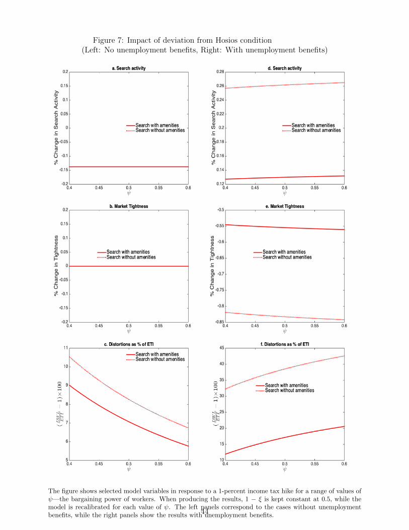
Figure 7: Impact of deviation from Hosios condition(Left: No unemployment benefits, Right: With unemployment benefits)

The figure shows selected model variables in response to a 1-percent income tax hike for a range of values ofψ—the bargaining power of workers. When producing the results, 1 − ξ is kept constant at 0.5, while themodel is recalibrated for each value of ψ. The left panels correspond to the cases without unemploymentbenefits, while the right panels show the results with unemployment benefits.44

on ds is negative, meaning that the consistent drop in s given higher taxes and across ranges

of ψ puts upward pressure on DWL.35 Of course, lower s means that congestion externalities

decrease for workers, but thick market externalities rise for firms. Therefore, lower s and

therefore upward pressure on DWL can be interpreted as suggesting that the worsening of

thick market externalities for firms outweighs the lessening of congestion externalities for

workers.

That said, the extent to which the ETI underestimates DWL decreases as ψ tends toward

1. The intuition behind this result is straightforward. As ψ tends toward 1, and with no

unemployment benefits, the search model’s outcome gets closer and closer to the neoclassical

outcome. This is because ψ = 1 implies that workers obtain all the surplus from a match,

just as they do in the neoclassical model. Therefore, with no unemployment benefits, as ψ

rises, the search model tends toward the neoclassical model, and, as shown earlier, in the

neoclassical framework, the ETI can potentially proxy perfectly for DWL. As such, with no

unemployment benefits, the ETI becomes a better proxy for DWL as ψ rises—this is also the

reason behind changes in DWL with positive unemployment benefits (panel f of the figure).

In the model with unemployment benefits, as shown in the right panels of Figure 7, search

activity always rises throughout the range of ψ values given an increase in taxes. That said,

in the case with unemployment benefits, as in Table 4, the coefficient on ds is positive.

This reflects the fact that the consistent rise in s puts upward pressure on DWL in face of

higher taxes and across ranges of ψ.36 Of course, higher s worsens congestion externalities

for workers but alleviates thick market externalities for firms. As such, the fact that changes

in s put upward pressure on DWL in this case can be interpreted as worsening in congestion

externalities for workers outweighing a lessening of congestion externalities for firms.

Also, recall from the earlier discussion that higher taxes trigger an increase in effective

wages in the case with unemployment benefits, which is what drives the increase in search

activity. However, higher effective wages ultimately result in firms posting fewer vacancies.

This, combined with the increase in search activity, means that the change in market tight-

35See equation 2.27.36See equation 2.27.

45

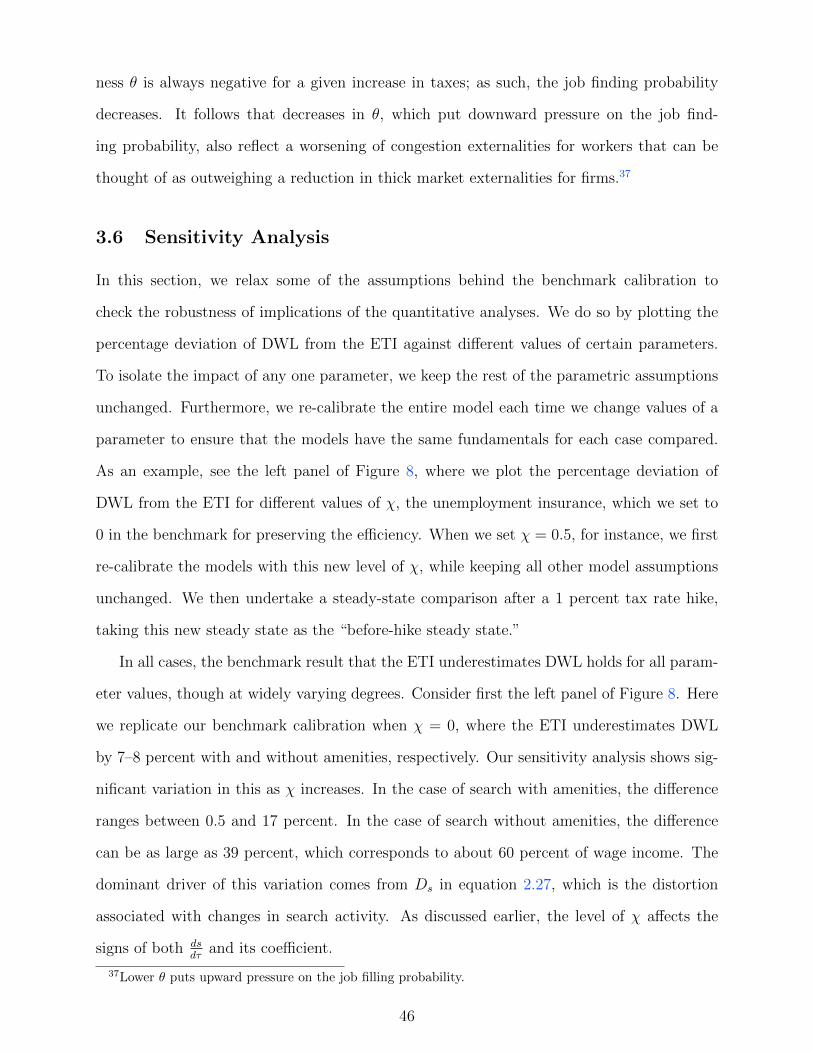
ness θ is always negative for a given increase in taxes; as such, the job finding probability

decreases. It follows that decreases in θ, which put downward pressure on the job find-

ing probability, also reflect a worsening of congestion externalities for workers that can be

thought of as outweighing a reduction in thick market externalities for firms.37

3.6 Sensitivity Analysis

In this section, we relax some of the assumptions behind the benchmark calibration to

check the robustness of implications of the quantitative analyses. We do so by plotting the

percentage deviation of DWL from the ETI against different values of certain parameters.

To isolate the impact of any one parameter, we keep the rest of the parametric assumptions

unchanged. Furthermore, we re-calibrate the entire model each time we change values of a

parameter to ensure that the models have the same fundamentals for each case compared.

As an example, see the left panel of Figure 8, where we plot the percentage deviation of

DWL from the ETI for different values of χ, the unemployment insurance, which we set to

0 in the benchmark for preserving the efficiency. When we set χ = 0.5, for instance, we first

re-calibrate the models with this new level of χ, while keeping all other model assumptions

unchanged. We then undertake a steady-state comparison after a 1 percent tax rate hike,

taking this new steady state as the “before-hike steady state.”

In all cases, the benchmark result that the ETI underestimates DWL holds for all param-

eter values, though at widely varying degrees. Consider first the left panel of Figure 8. Here

we replicate our benchmark calibration when χ = 0, where the ETI underestimates DWL

by 7–8 percent with and without amenities, respectively. Our sensitivity analysis shows sig-

nificant variation in this as χ increases. In the case of search with amenities, the difference

ranges between 0.5 and 17 percent. In the case of search without amenities, the difference

can be as large as 39 percent, which corresponds to about 60 percent of wage income. The

dominant driver of this variation comes from Ds in equation 2.27, which is the distortion

associated with changes in search activity. As discussed earlier, the level of χ affects the

signs of both dsdτ

and its coefficient.

37Lower θ puts upward pressure on the job filling probability.

46

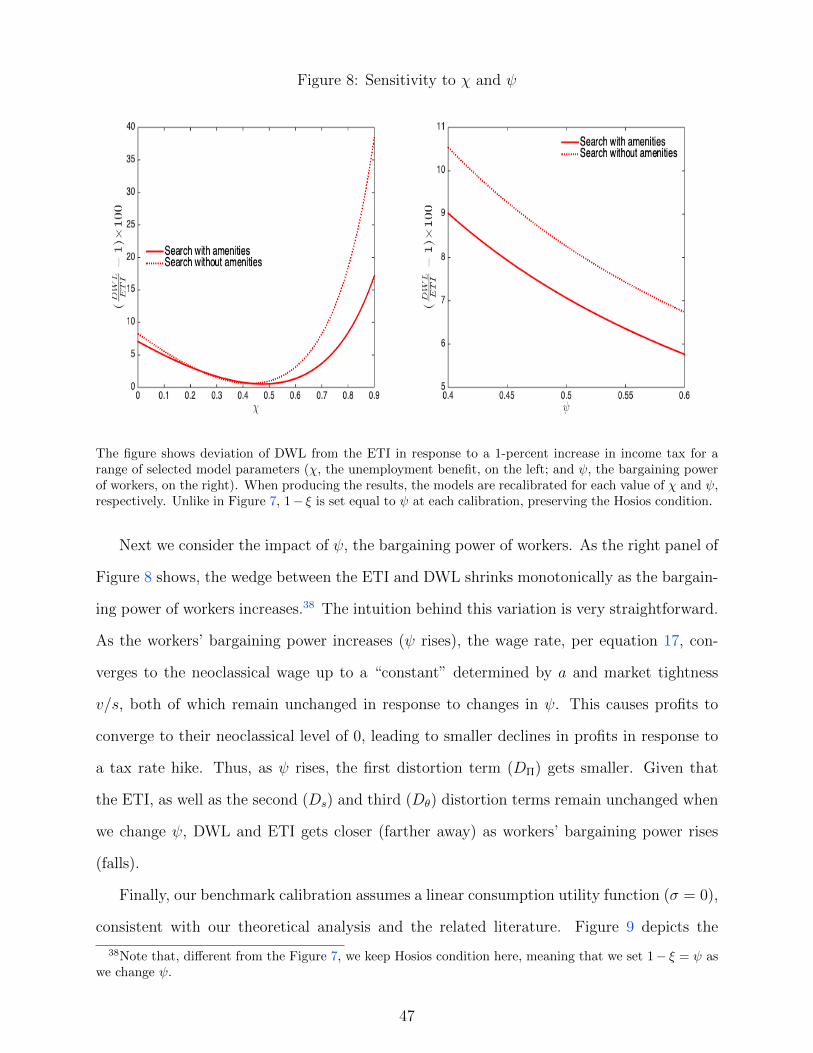
Figure 8: Sensitivity to χ and ψ

The figure shows deviation of DWL from the ETI in response to a 1-percent increase in income tax for arange of selected model parameters (χ, the unemployment benefit, on the left; and ψ, the bargaining powerof workers, on the right). When producing the results, the models are recalibrated for each value of χ and ψ,respectively. Unlike in Figure 7, 1− ξ is set equal to ψ at each calibration, preserving the Hosios condition.

Next we consider the impact of ψ, the bargaining power of workers. As the right panel of

Figure 8 shows, the wedge between the ETI and DWL shrinks monotonically as the bargain-

ing power of workers increases.38 The intuition behind this variation is very straightforward.

As the workers’ bargaining power increases (ψ rises), the wage rate, per equation 17, con-

verges to the neoclassical wage up to a “constant” determined by a and market tightness

v/s, both of which remain unchanged in response to changes in ψ. This causes profits to

converge to their neoclassical level of 0, leading to smaller declines in profits in response to

a tax rate hike. Thus, as ψ rises, the first distortion term (DΠ) gets smaller. Given that

the ETI, as well as the second (Ds) and third (Dθ) distortion terms remain unchanged when

we change ψ, DWL and ETI gets closer (farther away) as workers’ bargaining power rises

(falls).

Finally, our benchmark calibration assumes a linear consumption utility function (σ = 0),

consistent with our theoretical analysis and the related literature. Figure 9 depicts the

38Note that, different from the Figure 7, we keep Hosios condition here, meaning that we set 1− ξ = ψ aswe change ψ.

47

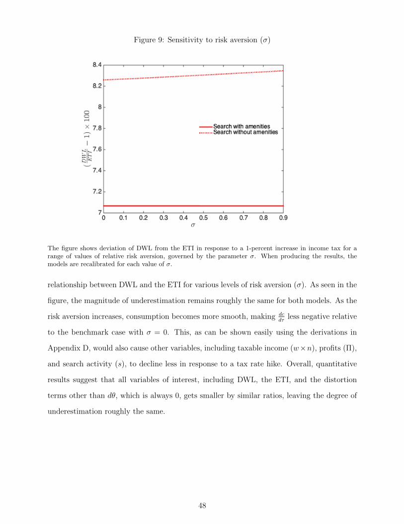
Figure 9: Sensitivity to risk aversion (σ)

The figure shows deviation of DWL from the ETI in response to a 1-percent increase in income tax for arange of values of relative risk aversion, governed by the parameter σ. When producing the results, themodels are recalibrated for each value of σ.

relationship between DWL and the ETI for various levels of risk aversion (σ). As seen in the

figure, the magnitude of underestimation remains roughly the same for both models. As the

risk aversion increases, consumption becomes more smooth, making dcdτ

less negative relative

to the benchmark case with σ = 0. This, as can be shown easily using the derivations in

Appendix D, would also cause other variables, including taxable income (w×n), profits (Π),

and search activity (s), to decline less in response to a tax rate hike. Overall, quantitative

results suggest that all variables of interest, including DWL, the ETI, and the distortion

terms other than dθ, which is always 0, gets smaller by similar ratios, leaving the degree of

underestimation roughly the same.

48

4 Conclusion

Governments almost exclusively rely on distortionary taxation for their revenue needs. These

taxes induce market participants to alter their behavior, often in substantial ways that reduce

social welfare. But just how costly is taxation? The answer is directly relevant to how much

taxation (and government spending) is optimally implemented.

Under some strong conditions in a stylized economic setting, social costs of taxation can

be inferred with knowledge of the ETI. A growing literature has characterized deviations

from this finding, emphasizing the role of externalities. Using a theoretical approach, we

revisit this result from the vantage point of a general equilibrium macroeconomic model

with labor search frictions. Employing a calibrated version of our model, we show that, in

this context, and against the backdrop of inefficient taxation, DWL can be up to 38 percent

higher than the ETI under a range of reasonable parametric assumptions. In addition, we

show that the divergence between DWL and ETI is widened in the presence of the typical

externalities that can arise in the context of frictional labor markets: congestion externalities

and thick market externalities.

That said, we characterize the information needed, in addition to the ETI, in order to

characterize DWL in the context of frictional labor markets. In particular, given a change in

taxes, this information includes, among other factors, levels and changes in job-finding and

job-filling probabilities, the extent to which workers and firms adjust their match-forming

behavior, and changes in profits, which, as is well known, are nonzero in typical labor-search

environments. Importantly, all of these factors have easily observable empirical counterparts.

Acknowledgements:

The views in this paper are solely the responsibility of the authors and should not be inter-

preted as reflecting the views of the Board of Governors of the Federal Reserve System or of

any other person associated with the Federal Reserve System.

49

References

Arseneau, D. M. and S. K. Chugh (2012): “Tax Smoothing in Frictional Labor Mar-

kets,” Journal of Political Economy, 120, 926–985.

Baily, M. N. (1978): “Some aspects of optimal unemployment insurance,” Journal of

Public Economics, 10, 379–402.

Barro, R. and H. Grossman (1971): “A General Disequilibrium Model of Income and

Employment,” American Economic Review, 61, 82–93.

Becker, D. (2011): “Non-wage job characteristics and the case of the missing margin.”

Working paper.

Chetty, R. (2006): “A general formula for the optimal level of social insurance,” Journal

of Public Economics, 90, 1879–1901.

——— (2009a): “Is the taxable income elasticity sufficient to calculate deadweight loss? The

implications of evasion and avoidance,” American Economic Journal: Economic Policy, 1

(2), 31–52.

——— (2009b): “Sufficient Statistics for Welfare Analysis: A Bridge Between Structural

and Reduced-Form Methods,” Annual Review of Economics, 1, 451–488.

Diamond, P. A. (1982): “Aggregate demand management in search equilibrium,” Journal

of Political Economy, 90 (5), 881–94.

Doerrenberg, P., A. Peichl, and S. Siegloch (2017): “The elasticity of taxable

income in the presence of deduction possibilities,” Journal of Public Economics, 151, 41–

55.

Epstein, B. and M. Kimball (2019): “The Decline of Drudgery and the Paradox of Hard

Work,” Mimeo.

Feldstein, M. (1999): “Tax avoidance and the deadweight loss of the income tax,” The

Review of Economics and Statistics, 81, 674–80.

50

Golosov, M., P. Maziero, and G. Menzio (2013): “Taxation and Redistribution of

Residual Income Inequality,” Journal of Political Economy, 121, 1160–1204.

Hall, R. E. and A. I. Mueller (2018): “Wage Dispersion and Search Behavior: The

Importance of Nonwage Job Values,” Journal of Political Economy, 126, 1594–1637.

Harberger, A. (1964): “The measurement of waste,” The American Economic Review,

54 (3), 58–76.

Hines, J. R. (1999): “Three Sides of Harberger Triangles,” Journal of Economic Perspec-

tives, 13 (2), 167–188.

Hosios, A. J. (1990): “On The Efficiency of Matching and Related Models of Search and

Unemployment,” Review of Economic Studies, 57, 279–298.

Hummel, A. J. (2019): “Unemployment and Tax Design,” Mimeo.

Hungerbuhler, M., E. Lehmann, A. Parmentier, and B. V. D. Linden (2006):

“Optimal Redistributive Taxation in a Search Equilibrium Model,” Review of Economic

Studies, 73, 743–767.

Kleven, H. J. and E. A. Schultz (2014): “Estimating taxable income responses using

Danish tax reforms,” American Economic Journal: Economic Policy, 6, 271–301.

Kroft, K., K. Kucko, E. Lehmann, and J. Schmieder (2020): “Optimal Income

Taxation with Unemployment and Wage Responses: A Sufficient Statistics Approach,”

American Economic Journal: Economic Policy, 12, 254–292.

Kydland, F. E. and E. C. Prescott (1982): “Time to Build and Aggregate Fluctua-

tions,” Econometrica, 50, 1345–1370.

Landais, C., P. Michaillat, and E. Saez (2018a): “A Macroeconomic Approach to

Optimal Unemployment Insurance: Theory,” American Economic Journal: Economic

Policy, 10, 152–181.

51

——— (2018b): “A Macroeconomic Approach to Optimal Unemployment Insurance: The-

ory,” American Economic Journal: Economic Policy, 10, 152–181.

Lavecchia, A. M. (2018): “Minimum Wage Policy with Optimal Taxes and Unemploy-

ment,” Tech. rep.

Lehmann, E., C. Lucifora, S. Moriconi, and B. Van der Linden (2016): “Beyond

the labour income tax wedge: the unemployment-reducing effect of tax progressivity,”

International Tax and Public Finance, 23, 454–489.

Lehmann, E., A. Parmentier, and B. Van der Linden (2011): “Optimal income

taxation with endogenous participation and search unemployment,” Journal of Public

Economics, 95, 1523–1537.

McDaniel, C. (2011): “Forces Shaping Hours Worked in the OECD, 1960-2004,” American

Economic Journal: Macroeconomics, 3, 27–52.

Michaillat, P. and E. Saez (2015): “Aggregate Demand, Idle Time, and Unemploy-

ment,” The Quarterly Journal of Economics, 130, 507–569.

——— (2019): “Optimal Public Expenditure with Inefficient Unemployment,” Review of

Economic Studies, 86, 1301–1331.

Mortensen, D. and C. Pissarides (1994): “Job creation and job destruction in the

theory of unemployment,” The Review of Economic Studies, 61 (3), 397–415.

Pierce, B. (2001): “Compensation Inequality,” The Quarterly Journal of Economics, 116,

1493?1525.

Pissarides, C. A. (2000): Equilibrium unemployment theory, The MIT Press.

Pissarides, C. A. and B. Petrongolo (2001): “Looking into the Black Box: A Survey

of the Matching Function,” Journal of Economic Literature, 39, 390–431.

Rosen, S. (1986): The theory of equalizing differences, Elsevier.

52

Saez, E. (2002): “Optimal Income Transfer Programs: Intensive versus Extensive Labor

Supply Responses,” The Quarterly Journal of Economics, 117, 1039–1073.

——— (2004): “The optimal treatment of tax expenditures,” Journal of Public Economics,

88, 2657–2684.

Saez, E., J. Slemrod, and S. Giertz (2012): “The elasticity of taxable income with

respect to marginal tax rates: a critical review,” Journal of Economic Literature, 50 (1),

3–50.

Shimer, R. (2005): “The Cyclical Behavior of Equilibrium Unemployment and Vacancies,”

American Economic Review, 95, 25–49.

——— (2012): “Reassessing the Ins and Outs of Unemployment,” Review of Economic

Dynamics, 15, 127–148.

Slemrod, J. (1998): “Methodological issues in measuring and interpreting taxable income

elasticities,” National Tax Journal, 773–788.

Slemrod, J. and S. Yitzhaki (2002): “Tax avoidance, evasion, and administration,” in

Handbook of public economics, Elsevier, vol. 3, 1423–1470.

Solon, G., R. Michaels, and M. W. L. Elsby (2009): “The Ins and Outs of Cyclical

Unemployment,” American Economic Journal: Macroeconomics, 1, 84–110.

Sullivan, P. and T. To (2014): “Search and nonwage job characteristics.” The Journal

of Human Resources, 49 (2), 472–507.

Weber, C. E. (2014): “Toward obtaining a consistent estimate of the elasticity of taxable

income using difference-in-differences,” Journal of Public Economics, 117, 90–103.

53

taxation, social welfare, and labor market frictions

Documents