taylor rule under financial instability · then, the “taylor rule” has become a tool of choice...
TRANSCRIPT
WP/08/18
Taylor Rule Under Financial Instability
Sofía Bauducco, Aleš Bulíř, and Martin Čihák

© 2008 International Monetary Fund WP/08/18 IMF Working Paper IMF Institute
Taylor Rule Under Financial Instability
Prepared by Sofía Bauducco, Aleš Bulíř, and Martin Čihák1
Authorized for distribution by Enrica Detragiache
January 2008
Abstract
This Working Paper should not be reported as representing the views of the IMF. The views expressed in this Working Paper are those of the author(s) and do not necessarily represent those of the IMF or IMF policy. Working Papers describe research in progress by the author(s) and are published to elicit comments and to further debate.
This paper contributes to the analysis of monetary policy in the face of financial instability. In particular, we extend the standard new Keynesian dynamic stochastic general equilibrium (DSGE) model with sticky prices to include a financial system. Our simulations suggest that if financial instability affects output and inflation with a lag and if the central bank has privileged information about credit risk, monetary policy that responds instantly to increased credit risk can trade off more output and inflation instability today for a faster return to the trend than a policy that follows the simple Taylor rule with only the contemporaneous output gap and inflation. The long-run impact on consumption from the augmented policy rule appears negligible, however. JEL Classification Numbers: E52, E58, G21 Keywords: monetary policy rule, financial instability, DSGE models Author’s E-Mail Address: [email protected]; [email protected]; [email protected]
1 Sofía Bauducco (Universitat Pompeu Fabra) visited the IMF in 2007. The paper benefited from comments by Enrica Detragiache and IMF seminar participants. All remaining errors are those of the authors.
2
Contents Page
I. Introduction ............................................................................................................................3
II. How Do Central Banks Really Determine Monetary Policy Under Financial Instability? 4 A. The Absence of the Financial Sector from Monetary Policy Models.............................. 4 B. Evidence on Financial Instability and Central Banks ...................................................... 5
III. The Model............................................................................................................................7 A. Households....................................................................................................................... 8 B. Goods Firms (“Firms That Do Not Need External Financing”) ...................................... 9 C. Innovative Firms (“Firms That Need External Financing”)............................................. 9 D. Financial Intermediaries................................................................................................. 10 E. Technology ..................................................................................................................... 11 F. The Central Bank............................................................................................................ 12
IV. Model Simulations.............................................................................................................14 A. Parameterization............................................................................................................. 14 B. Simulation Results.......................................................................................................... 15 C. Welfare Calculations ...................................................................................................... 18
V. Practical Issues and Possible Extensions ............................................................................19
VI. Conclusions........................................................................................................................21
References................................................................................................................................23
Appendix..................................................................................................................................26 Figures 1. Distribution of Returns of Innovative Firms........................................................................33 2. Shock to Exogenous Technology.........................................................................................34 3. Shock to Exogenous Technology: Response of Output, Output Gap, Inflation, and Labor .............................................................................................................35 4. Shock to Exogenous Technology: Response of Policy Rate, Real Interest Rate, Loan Rate, and Effective Deposit Rate .................................................36 5. Shock to Exogenous Technology: Response of tω , Endogenous Technology and Total Technology ......................................................................................37 6. Shock to Probability of Default ...........................................................................................38 7. Shock to Probability of Default: Response of Output, Output Gap, Inflation, and Labor .............................................................................................................39 8. Shock to Probability of Default: Response of Policy Rate, Real Interest Rate, Loan Rate, and Effective Deposit Rate .................................................40 9. Shock to Probability of Default: Response of tω , Endogenous Technology and Total Technology ......................................................................................41
3
“[A] reaction function in which the real funds rate changes by roughly equal amounts in response to deviations of inflation from a target of 2 percent and to deviations of actual from potential output describes reasonably well what this committee has done since 1986.”
Janet Yellen at the January 1995 FOMC
“[S]imple instrument rules at most explain two-thirds of the empirical variance of interest rate changes.”
Lars E.O. Svensson (2003)
I. INTRODUCTION
How should changes in financial sector soundness affect monetary policy? In this paper, we answer this question by addressing two simplifications in the standard monetary dynamic stochastic general equilibrium (DSGE) model: (i) the omission of a financial system, and (ii) the omission of forward-looking variables in the policy (Taylor) rule. In our model, the central bank has privileged information about the health of the financial system, a reasonable assumption given that many central banks are involved in financial sector supervision, and even those that are not have access to a wealth of payment system data. Our simulation results show that if the central bank responds to a deterioration in the credit risk faced by the financial system by monetary easing, using an augmented rule, such a “preemptive strike” stabilizes inflation and output better in the short run than the simple Taylor rule that is usually assumed in the DSGE model. In other words, well-informed, forward-looking discretionary policymaking, that takes into account the default rate of financial intermediaries’ lending projects and its impact on future output developments, is preferable to simple backward-looking rules.
These findings have both positive and normative implications. As regards positive implications, the findings provide model justification for the existing central bank practice of intervening against a background of financial shocks—the simple rule is an inaccurate description of central bank behavior, generally underestimating the actual policy changes. The central bank following our augmented policy rule trades off more output and inflation instability today for a faster return to the trend path tomorrow. As regards normative implications, the simulations suggest limits to the use of monetary policy instruments for such financial system stabilization, namely the size and duration of the financial shock. The central bank seems capable only of a faster reaction to the financial instability shock, keeping the nature of monetary policy unchanged and long-run consumption volatility remains practically identical under both rules. Moreover, monetary easing is unlikely to work in economies with either fixed exchange rates or a strong exchange rate channel of monetary transmission.

4
The paper is organized as follows. Section II reviews the recent literature on the link between monetary policy and financial sector instability. In Section III, we build a DSGE model with financial intermediaries and an augmented policy rule. In Section IV, we calibrate the model on U.S. data and present simulations from the model for a range of policy-relevant shocks. In Section V, we discuss possible extensions of the model. Section VI concludes.
II. HOW DO CENTRAL BANKS REALLY DETERMINE MONETARY POLICY UNDER FINANCIAL INSTABILITY?
In a widely quoted paper, Taylor (1993) suggested that monetary policy could be explained by a straightforward rule that links the central bank's policy rate to contemporaneous deviations of inflation and output from their target and potential levels, respectively. Since then, the “Taylor rule” has become a tool of choice for analysts, researchers, and central bank staff needing to model central bank responses to macroeconomic developments. However, it remains doubtful whether the simple, backward-looking rule—which can explain only up to two-thirds of the empirical variance of policy rate changes—is an accurate description of central banks’ behavior (e.g., Svensson, 2003).
A. The Absence of the Financial Sector from Monetary Policy Models
The financial system is conspicuously absent from the standard monetary dynamic stochastic general equilibrium (DSGE) model as well as from simpler models built for policy purposes. In fact, a typical model used by an inflation-targeting central bank does not consider banks at all and its policy rule ignores the health of the financial system. Such an omission seems puzzling, given that many central banks have financial stability as an explicit policy goal (Crockett, 1997) and that considerable time and energy are devoted by central bankers to discussing and analyzing the financial sector.2
Whether financial sector concerns should in fact influence monetary policy decisions has remained a controversial issue. On the one hand, economists such as Schwartz (1995) argued that by vigorously pursuing the goal of price stability, central banks would promote financial stability the best. Any information about the financial system is useful only to the extent that it can be used to improve the inflation forecast, while fine-tuning the policy rate to meet other objectives may do more harm than good. On the other hand, central bankers argued that financial systems are inherently fragile and central banks need to intervene when financial institutions are under stress. According to this view, restricting monetary policy to price stability considerations alone is incorrect and policymaking would be improved by incorporating financial sector concerns explicitly in the rule (Bernanke and Gertler, 1999,
2 Financial instability is a leading indicator of the business cycle (Borio, 2006), and output costs of financial instability are estimated to be around 1 percent of GDP annually (Henry, 2004). The increasing importance that central banks attribute to financial stability can be illustrated by the rapidly growing number of financial stability reports published by central banks (see Čihák, 2006, for a review).
5
and Cecchetti and others, 2000). These interventions can be either proactive, in the spirit of “pricking the bubbles” or “counteracting irrational exuberances” that have not yet resulted in unfavorable financial sector developments, or reactive, adjusting the monetary stance in response to observed unfavorable financial sector developments.3
Central banks may also react to financial sector problems for reasons unconnected to monetary policy. Some central banks have a role in prudential supervision of banks or other financial institutions and may be perceived to be responsible for the soundness of the supervised institutions, including ensuring the smooth functioning of the payment and settlements systems. Owing to regulatory and supervisory agencies’ lack of independence, regulatory and monetary policy objectives may become intertwined, with the latter being subordinated to the former (Quintyn, 2007).
B. Evidence on Financial Instability and Central Banks
A host of recent empirical studies have found that central banks react to financial sector instability, but that their reaction is asymmetric, nonlinear, and reflects the nature of the underlying shock. Surprisingly, empirical results and anecdotal evidence on the link between financial instability and monetary policy have been largely ignored in theoretical papers.
Borio and Lowe (2004) estimate empirically modified Taylor rule functions for Australia, Germany, Japan, and the United States, concluding that “central banks either do not respond much to financial imbalances or, to the extent that they do, they respond asymmetrically. Policy appears to be loosened in the face of the unwinding of imbalances beyond what would be suggested by the behavior of inflation and the output gap alone, but does not seem to be tightened as imbalances build up.” In other words, they find evidence of a reactive monetary policy, but no evidence of a proactive policy. The authors measure financial instability using credit and equity-price gaps, i.e., deviations from a Hodrick-Prescott filter.
Bordo and Jeanne (2002) argue that the reactive policy of injecting liquidity ex post in the event of a credit crunch may in certain circumstances be more costly in terms of lost output than a proactive policy incorporating asset prices directly into the central bank’s objective function. They support their simple model with empirical simulations for episodes such as the Great Depression or the asset-price boom in Japan. However, their stylized model limits central banks to either “pricking the bubble” or “an after-crisis cleanup.” This seems to be an unduly narrow scope for monetary policy adjustments since a forward-looking central bank would presumably adjust its stance before a crisis erupts. Moreover, the cleanup phase is not
3 For a discussion on the merits of proactive and reactive interventions see the general discussion of Borio and White (2003) at http://www.kc.frb.org/PUBLICAT/SYMPOS/2003/pdf/GD32003.pdf. The participants were split whether either extension is desirable, seeing both of these interventions as representing “second-best” policies as compared to the “first-best” policy of price stability.
6
really interesting as the scope for any change in the monetary stance during a crisis is limited (Boorman and others, 2000).
Cecchetti and Li (2005) find that policymakers react to the state of their banking system’s balance sheet, attempting to counteract or even neutralize the procyclical effect of prudential capital regulation. The resulting disintermediation has a procyclical effect and the authors conclude that ”for a given level of economic activity and inflation, the optimal policy reaction dictates setting interest rates lower the more financial stress there is in the banking system when the economic activity is in the downturn.” There are two problems with the Cecchetti and Li results: (i) central bank reaction is conditioned on the business cycle only; and (ii) the capital adequacy requirement is an unlikely candidate as a financial instability measure.
Bulíř and Čihák (2007) estimate a modified Taylor rule in a quarterly panel of 28 industrial and emerging market countries using a battery of seven alternative measures of financial instability and find that, irrespective of the definition used, instability has been associated with short-term interest rates below those implied by the simple rule. Moreover, the responsiveness of monetary policy to domestic financial sector vulnerability appears to be stronger in closed economies and in economies where banking supervision is inside the central bank. Quantitatively, in a country with a freely floating exchange rate, the contemporaneous impact of a one standard deviation increase in the “probability of crisis” variable is associated with interest rates that are about 0.2 percentage points below what they would be otherwise.
The literature on DSGE models has largely neglected the role of financial intermediaries in the economy. The most widely used models usually do not include a financial sector and, if they do, its role is solely to produce transaction services. Nevertheless, there have been some valuable attempts to introduce this element into the analysis. Williamson (1987) constructs a business cycle model in which financial intermediation is a determinant of business cycle fluctuations. In his model, banks exist because of asymmetric information and costly monitoring. Stochastic disturbances to the riskiness of investment projects produce equilibrium business cycles in the presence of monitoring costs: cycles are produced through costly intermediation rather than firms’ failures. There are two mechanisms through which real output fluctuates when there are stochastic disturbances. One is an intertemporal substitution mechanism, common to many real business cycle models. The other is a credit supply effect: a reduction in the amount of loans in the current period reduces the next period’s output. Though the general idea of the paper is close to ours, the model does not incorporate nominal rigidities (sticky prices) and fails to consider the role of monetary policy in smoothing fluctuations in the cycle.
Bernanke, Gertler and Gilchrist (1998) develop a new Keynesian model that includes a partial equilibrium model of the credit market in order to study how credit market frictions amplify real and nominal shocks to the economy. In the model, banks act as intermediaries
7
between households, which hold deposits, and entrepreneurs, which ask for loans in order to produce a homogeneous good. Their framework exhibits a “financial accelerator”, in the sense that endogenous developments in credit markets propagate and amplify shocks to the economy. As in the case of Williamson, the friction in the credit market arises due to the presence of asymmetric information and agency costs. The model does not incorporate any concept of financial instability and banks are able to diversify idiosyncratic shocks completely and, thus, the ex ante and ex post deposit rates are identical.
Finally, Brousseau and Detken (2001) exploit a sunspot equilibrium in a standard new Keynesian framework. In their model, the central bank may choose not to keep inflation at target in the short term in order to stabilize the financial system. They interpret the sunspot shock as financial instability because its variance is linked to a change in the policy rate. The larger the change in the policy rate, the higher the next period’s variance of the sunspot process and the simple monetary policy rule is no longer optimal. The authors provide neither an explicit modeling of the financial sector nor a clear description of the process by which financial instability affects the rest of the economy. In fact, the sunspot shock does not influence the vector of endogenous variables and the shock brings indeterminacy to the otherwise standard model. The model does not consider the use of a Taylor rule by the central bank but, instead, discusses the specification of the optimal policy with respect to the one arising from the standard model.
III. THE MODEL
Our model, which builds on Galí (2002), addresses two simplifications in the standard new Keynesian dynamic stochastic general equilibrium (DSGE) model: the omission of a financial system and the omission of forward-looking variables in the policy rule. We differ from a Galí-type DSGE model in two respects: (i) financial intermediaries supply external financing to some firms; and (ii) firms that are sensitive to the supply of loans and the interest rate are linked with the rest of the firms in the economy through a productivity nexus.
These innovations capture a number of well-accepted stylized facts that have been absent from the typical DSGE model used in the literature.4
• The credit channel works through a subset of firms that depend on external financing.
• Small- and medium-sized firms depend on banks for external financing much more than large firms.
• Small, start-up firms perish easily if they cannot obtain external financing.
4 Needless to say, these elements have been absent also from the earlier generations of models that preceded the class of DSGE models, including those used by most central banks. See Bernanke, Gertler, and Gilchrist (1998) and Fukač and Pagan (2006) for reviews.
8
• Large firms rely on small firms to bring about technology and productivity improvements.
• Higher lending rates make both the marginal loan and the lending portfolio of the financial system more risky.
• The central bank can observe the health of the financial system one period before the public does.
• Monetary policy actions do not result in moral-hazard behavior by banks.
The economy contains five types of agents: households; goods-producing firms that are monopolistic competitors; innovative firms that are freely competitive; financial intermediaries, which are freely competitive as well; and a central bank. While we describe them in turn below, further details of the derivations are provided in the Appendix.
A. Households
The economy is populated with a continuum of infinitely-lived and identical households that derive utility from consumption of goods and leisure, and invest their savings in a financial intermediary that pays a nominal rate tr for one-period deposits made at time t-1. Households consume a basket of all goods available according to
1 1 1
0
( )t tc c i di
εε εε− −⎡ ⎤
= ⎢ ⎥⎣ ⎦∫ ,
where c is the contemporaneous consumption of the representative household andε is the elasticity of substitution between any two given goods indexed i and i’.
The problem of the representative household can be written as
, 0max ( , )
t t
to t tc n t
E U c nβ∞
=∑ ,
subject to its period-by-period budget constraint (in nominal terms)
tttttttttttttt TPPdPrnwPdPcP +Π++=+ −− 11 ,
where td are deposits, tw is the wage rate, tn is labor, tΠ are dividends, and tT are lump sum taxes; all these variables are in real terms.
9
B. Goods Firms (“Firms That Do Not Need External Financing”)
The first segment of the corporate sector contains a continuum of infinitely-lived firms acting as monopolistic competitors. These firms produce their single perishable, differentiated good with a technology
)()( jnajy ttt = ,
where ta is a technology shifter common to all firms. The economy-wide, competitive factor market guarantees that all firms pay the same nominal wage ttt wPW = for a unit of labor employed. The key distinguishing feature of these firms is that they do not need to borrow from financial intermediaries and finance themselves through retained earnings.
Following Calvo (1983), we assume that these firms adjust their prices infrequently and that the opportunity to adjust prices follows an exogenous Poisson process. Each period there is a constant probability θ−1 that the firm will be able to adjust its price, independently of past history. Inability to adjust prices every period is the source of nominal rigidities that make inflation distortionary.
C. Innovative Firms (“Firms That Need External Financing”)
The non-financial corporate sector contains also firms that have to borrow from financial intermediaries to develop a project. These firms only live for two periods and operate under perfect competition. The key distinguishing feature of these firms is that, unlike the goods firms, they are dependent on external financing. In period t such a firm invests in a project in order to obtain a return in period t+1. The technology is such that
)()()(1 jsjjs tt χ=+ . (1)
where )( jst is the initial investment made by firm j in the project and )( jtχ is the firm-specific return of the project.
Some of these firms survive and some do not. For simplicity, we assume that a constant fraction γ of these firms born in period t survive with probability one in period t+1. Moreover, to capture the trade-off between risk and return, we assume that firms that survive with probability one, i.e., “risk-free” firms, are the least profitable firms. The remaining firms may die at the beginning of period t+1 with probability 1+tδ , where 1+tδ is stochastic. A firm that does not survive obtains a zero return for its project. Finally, 1+tδ is realized only at the beginning of period t+1, after firms have applied for and received loans.
The returns of innovative firms are nonstochastic, firm-specific, and distributed according to a log-normal distribution with parameters μ andσ . We index firms according to their
10
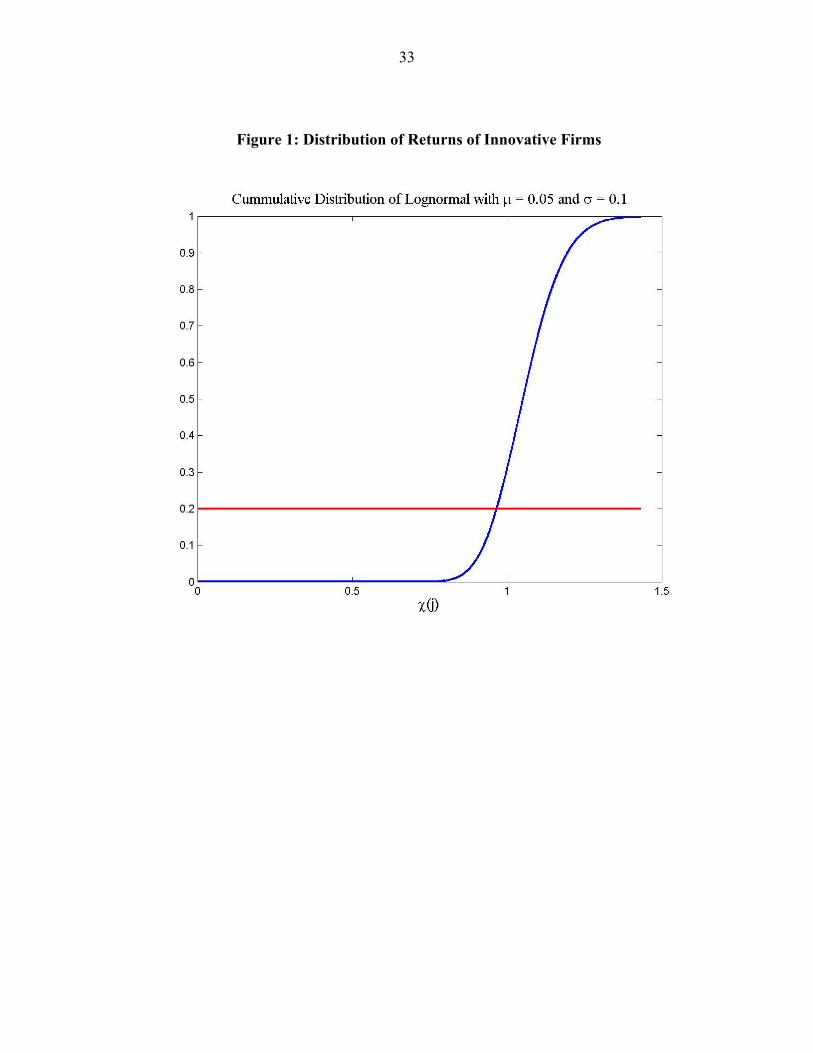
returns in the interval [0, 1], denoting with 0 the firm for which min)( χχ =j and with 1 the firm for which max)( χχ =j . We establish a one-to-one correspondence between the firm’s index and the lognormal cumulative distribution function. That is, firm j is such that a proportion j of firms obtain returns which are lower than )( jχ . Then γ is both the proportion of firms that survive with probability one next period and the most profitable non-risky firm. Figure 1 shows a stylized distribution of returns with parameters 05.0=μ ,
1.0=σ , and 2.0=γ . Firms that obtain returns higher than 9664.0)( =γχ are risky, in the sense that they may die next period with probability 1+tδ . On the contrary, firms with returns lower than 9664.0)( =γχ survive with probability one. In Section IV we will show results under different assumptions aboutγ .
D. Financial Intermediaries
The economy also contains a continuum of financial intermediaries that act as go-betweens for households and innovative firms. As there is free entry in the financial sector, banks obtain zero profits in equilibrium. These institutions receive deposits from households in period t and lend to innovative firms, charging for them a lending rate tz . At time t+1 firms that have survived repay their loans and intermediaries pay to households the return rt+1. For simplicity, we assume zero recovery on loans to failed firms. We will assume that intermediaries are able to monitor whether a firm exists or not without a cost, but cannot distinguish between firms and thus charge the same loan rate tz to all firms. However, a firm j has an incentive to ask for a loan only if its expected project return is higher than the lending rate. In other words, there is no moral hazard problem in the model.
tzj >)(χ . (2)
We assume that tzt ∀< maxχ . Therefore, the marginal firm tω to ask for a loan will be such that
tt z=)(ωχ .
In Figure 1 the marginal-firm cutoff point tω can be interpreted as the proportion of innovative firms that have returns lower than tz and, therefore, do not find it profitable to apply for a loan. Thus, due to the lack of funds, these firms will not be producing in period t+1. Conversely, the proportion of firms asking for loans will be tω−1 .
Given the technology of innovative firms, a firm for which equation (2) holds has an infinite demand for loans. Since banks cannot distinguish among firms, they will divide their loanable resources (household deposits) into equal parts and provide the same amount of
11
loans to each firm that asks for one: t
tt
dl
ω−=
1. This simple assumption has a profound
implication: the riskiness of the whole loan portfolio is increasing in the lending rate. At higher rates fewer firms apply for a loan and the lending portfolio becomes more concentrated in the high-return/high-risk segment and thus more risky overall.
Intermediaries’ opportunity cost of a loan is a central bank bill that pays a nominal interest rate equal to ti (policy rate) and that is for all practical purposes equivalent to short-term treasury bills. Then it has to be the case that the return on lending to firms is equal to the return on investing in the central bank paper and the loan rate will be determined as the rate such that the expected returns from loans are equal to the interest rate ti .5
)~( 1+= ttttt lzEdi , (3)
where 1~+tl are loans that are actually repaid in period t+1. Notice that, since banks do not
know the probability of firm survival at the moment they lend to them, they compute the loan rate based on their expectations of the shock to 1+tδ . The ex post deposit rate will be thus:
tttt dlzr /~11 ++ = .
In other words, if a smaller proportion of loans are repaid in t+1, the (ex-post) deposit rate becomes smaller, which means an increase in the spread between the deposit rate on one hand and the policy rate and the lending rate on the other hand.
E. Technology
The economy-wide total technology ta consists of two components. One component is exogenous and stochastic and follows an autoregressive process
at
st
ast aa ερ += −1
))
where atε is an independent and identically-distributed (i.i.d.) shock and s
ta) denotes log-
deviations of sta from steady state.
5 We assume that there is perfect competition and free entry in the intermediaries market, and that intermediaries are risk neutral. Therefore, no bank would charge a higher rate for loans since this would imply that some other intermediary could charge a smaller rate and capture all the demand for loans. Similarly, no bank would be willing to charge a smaller rate than ti because it could buy the central bank paper that yields a higher return. Since banks are risk neutral, they will charge a rate for loans such that their expected returns from loans equal their opportunity cost ti . Provided that there is free entry in the market, profits will be equal to zero.
12
The other, additional components of technology are the projects developed by the innovative firms that asked for loans in period t-1 and survived in period t. The production function for this type of technology is
( )11 1
*
1
)()(−−
⎥⎥⎦
⎤
⎢⎢⎣
⎡= ∫
−
ττ
ω
ττ
δ djjjsat
ttit ,
where 1)(* =jtδ if the firm survived in period t and zero otherwise, and τ is the elasticity of substitution between any two projects j and j’. Substituting (1) into the last expression and rearranging, we obtain
( )1
111 1
*
1)()(
1 −
−−−
−⎥⎥⎦
⎤
⎢⎢⎣
⎡= ∫
− t
tt
it
ddjjja
tω
δχττ
ω
ττ
,
Finally, total technology combines both the exogenous and endogenous components according to a Cobb-Douglas function
αα −=
1st
itt aaa ,
where α is the contribution of technology generated by innovative firms, ita , to total
technology. Thus, without innovative firms, productivity growth would be limited to the exogenous component only.
F. The Central Bank
The central bank seeks to stabilize the economy, which means that it responds to the productivity and survival shocks that hit the two types of firms ( s
ta and tδ , respectively). We examine two central bank response functions.
First, we look at a central bank that employs the traditional Taylor rule to set its instrument, a policy rate:
t t x ti xπφ π φ= +) ) (4)
where ti is the policy rate, tπ) is inflation in period t and tx is the output gap, defined as the
difference between actual output and natural output (that is, output in the flexible price allocation). In order to guarantee a unique equilibrium, the rule needs to be such that πφ >1.
13
Second, we look at a central bank that continually monitors financial intermediaries and their counterparts to infer the state of the economy and the impact of financial institutions’ health on the real economy. This information is likely to be collected through prudential supervision of financial intermediaries (if the central bank has prudential powers), or through the central bank’s role in the payment system. This information is confidential, i.e., exclusive to the central bank. While individual financial institutions would have detailed information about their clients, possibly better than that available to the central bank, the central bank is likely to be the only one to have such information for the financial system as a whole.
Empirical studies suggest that if central banks have recent supervisory information from on-site visits, they can achieve better predictions of financial stability than is possible based on publicly available data.6 If the central bank has this information, it can use it to improve the stabilization outcomes. In particular, if the chances of firm survival are good, the usual Taylor rule would apply. However, if the chances are not as good and the central bank has private information on tδ at the beginning of period t, it may decide to incorporate this information in the rule. This means that the central bank’s policy response function would look as follows
⎩⎨⎧
−+++<−+
=++
++
otherwise))((ˆ0)( ifˆˆ
11
11
ttttxt
ttttxtt Ex
Exi
δδνφφπφδδφπφ
δδπ
π (5)
where 0<δφ and δν is either a positive or negative shock to the sensitivity of the rule to deviations of tδ , capturing both the reporting lags in financial stability reports and the policymaker’s nonlinear and asymmetric response to deviations of tδ . Note that, if equation
(5) did not include the shock δν , knowing πφ , xφ and δφ agents would be able to infer tδ from the interest rate set by the central bank and the existence of signal extraction would defy the policymaker’s private information. One could also think that the central bank cannot perfectly foresee tδ and only receives more information to compute the conditional expectation than the rest of the agents in the economy. Nevertheless, under this specification the qualitative implications of our setup will remain unchanged.
6 For example, Berger, Davies, and Flannery (2000) find, using U.S. data, that if supervisory inspections were recent, assessments based on those inspections tended to be more accurate than equity and bond market indicators in predicting future changes in the performance of large bank holding companies. The relative predictive power of supervisory data is even higher in economies with lower public availability of data on financial soundness of banks. For instance, Bongini, Laeven, and Majnoni (2002) arrive to a similar, but stronger result for banks in East Asia during the 1996–98 crisis.
14
The timing of events will be as follows: at the beginning of every period, after tδ and sta are
realized, total technology ta is observed. Households make their decisions on consumption, saving, and labor allocations, forming their expectations based on the information they possess at the time. The central bank sets the policy rate according to the simple rule (4) in the benchmark scenario; while it employs the augmented rule (5) in the alternative scenarios, using also different values of this information in the rule ( δφ ). Therefore, in (5) the central bank uses information that the rest of agents do not possess and we want to study whether this informational advantage is relevant for the determination of the policy rate or not.
In what follows, we will calibrate the model and observe the effects of two shocks on the economy: (i) a pure technological shock; and (ii) a shock to the probability of survival of firms. We will study two different scenarios: first, the benchmark, in which the Taylor rule is defined as in (4), with the parameter values πφ =1.5 and xφ =0.5 used in Taylor (1993) and many of the subsequent papers, and second, a scenario in which the policy rule is as in (5) with 5.0−=δφ . This parameterization of δφ is somewhat arbitrary, but the results do not differ qualitatively if we use, for example 25.0−=δφ or 75.0−=δφ . What matters from a qualitative standpoint is that 0<δφ .
IV. MODEL SIMULATIONS
We calibrate the model and observe the effects of two shocks: a pure technological shock and a shock to the probability of survival of firms. The time period is one quarter.
A. Parameterization
We calibrate the model using parameter values from Bernanke, Gertler and Gilchrist (1998) and Galí (2001), both of which refer to the U.S. economy. We use the following utility function for households:
ϕσ
ϕσ
+−
−=
+−
11),(
11tt
ntnc
ncU
with 1== ϕσ . The probability of adjusting prices in a given period θ−1 is set equal to 0.25, which implies average price duration of one year, a value in line with survey evidence. The discount rate β is set to be 0.99. The serial correlation for the technology process, aρ , is assumed to be 0.95.
The process for the probability of small-firm survival is
δδ εδρδδ ttt ++= −1
15
where δε t is an i.i.d. process.
Given the average duration of post-war U.S. recessions of 11 months, we choose δρ to be 0.25 and the annual rate of business failure, δ , is equal to 0.03, approximating the data. The share of firms that survive for sure,γ , is chosen to be 0.2, which implies a quarterly steady-state spread between loan and deposit rates of 0.76 percent and an annual loan rate of 7.28 percent.
The variances of the technological shock and probability-of-survival shocks, aσ and δσ , are assumed to be 0.01 and 0.0025, respectively. The last two parameters, the participation of i
ta in the creation of technology and the elasticity of substitution between any two projects j and j’, are set to equal 05.0=α andτ = 4/3, respectively. That is, we are assigning a comparatively small role of i
ta in the creation of total technology, but—based on U.S. data—we expect sizeable effects from shocks to the probability of default.
To assess robustness of our results, we have calculated our simulations with a range of different distributions of returns to innovative firms. The general results do not vary substantially. For exposition purposes, we choose a lognormal distribution with parameters
05.0=μ and 1.0=σ .
B. Simulation Results
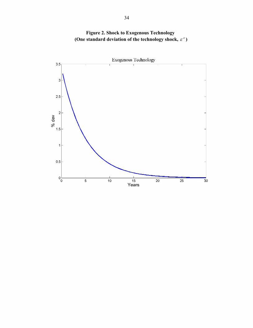
An exogenous technology shock
First, we simulate an exogenous technology shock, that is, a positive shock in sta equal to its
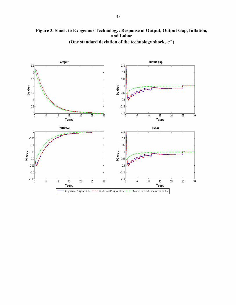
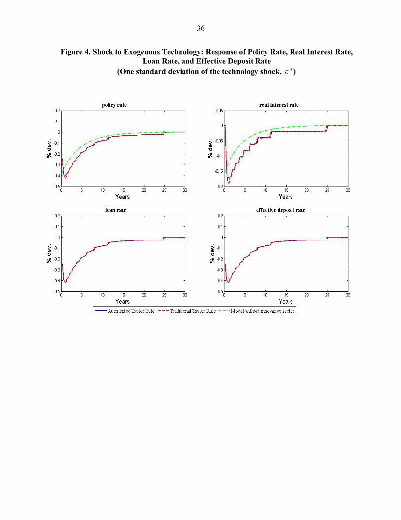
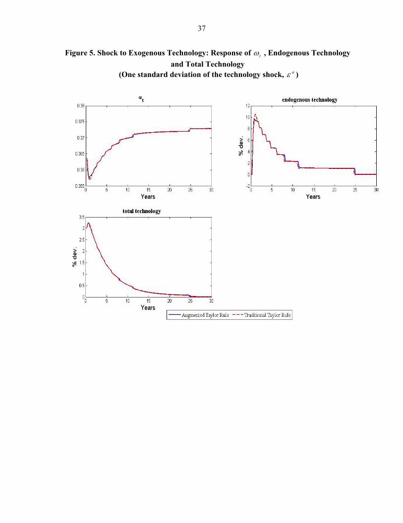
one standard deviation ( aε ). Figure 2 shows the trajectory of the shock, Figure 3 shows the response of output, output gap, inflation and labor, Figure 4 shows the evolution of the main interest rates (policy rate, deposit rate, loan rate, and effective (ex post) deposit rate) and finally Figure 5 shows the evolution of loan application ( 1−tω ) and endogenous and total technology.
Both in Figure 3 and Figure 4 we compare the results from our model (with both specifications of the Taylor rule given in equations (4) and (5)) with what is obtained in a standard model without the innovative sector. This last case has been widely studied in the literature and will serve as a benchmark for comparison purposes. In Figure 5, we do not show results for the benchmark model since the variables graphed do not appear in such a framework.
A positive exogenous technology shock in an economy with sticky prices, imperfect competition, and no innovative sector generates lower employment, higher output, and opening of the output gap, as depicted by the alternating dashed green line in Figure 3. While all firms experience a decrease in their marginal costs, not all can adjust their prices in this
16
period (Galí, 2001).Thus, the consequent changes in the aggregate price level and demand will be proportionately less than the initial increase in productivity.
In the above economy, the responses of the variables to an exogenous technology shock are both different from the simple benchmark model and more pronounced. Despite the differences explained below, from period 2 on the qualitative response of all variables is identical in all three scenarios. The response of labor and the output gap in the first period is positive, becoming negative only from the second period onwards. This result follows from the initial monetary loosening based on the central bank’s private information. The path of the variables is not as smooth as before, and for some variables such as labor and output gap the response is not even monotonic. This result follows from the impact of lending conditions on the evolution of endogenous technology.
Increased volatility results from the presence of endogenous technology and bank lending. Recall that:
( )1
111 1
*
1)()(
1 −
−−−
−⎥⎥⎦
⎤
⎢⎢⎣
⎡= ∫
− t
tt
it
ddjjja
tω
δχττ
ω
ττ
From this expression, we can observe that the creation of endogenous technology in period t depends on the proportion of firms applying for a loan 1−tω and deposits 1−td . The higher the level of deposits, the higher the amount of the loan received by each firm and, consequently, the higher the contribution of technology generated by innovative firms, i
ta . The effect of
1−tω on ita is a priori indeterminate: while a lower 1−tω implies that more firms are obtaining
loans and thus the term in brackets increases, the total amount of deposits has to be divided
over a higher number of borrowers (1
1
1 −
−
− t
tdω
decreases ).
More specifically, the decrease in the policy rate due to the negative response of inflation causes loan applications to decrease on impact, whereas deposits increase because of the better expectations on future consumption (see (A14) in the appendix). The full impact on endogenous technology is positive; nevertheless, this effect only takes place in period 2. This translates into a higher expectation of output (and consequently, consumption) for period 2, which causes period 1 consumption to increase more than what is accounted by the period 1 increase in exogenous technology. Thus, labor increases, causing the output gap to increase as well (A6). From period 2 onward the higher level of endogenous technology is added to the original effect of the exogenous technology shock, which explains the amplified response of all variables to the shock.
17
As the technology shock dies out, loan applications, tω , increase and deposits, 1−td , decrease
until they reach their steady state values. Nevertheless, the path of ita is not monotonic:
while the overall trend is downward sloping, in some periods it increases with respect to its value in the previous period. This is so because the process for i
ta has no memory (there is
no transmission from ita 1− to i
ta as innovative firms live for two periods only) and the effect
of 1−tω on ita is indeterminate a priori.
Nevertheless, the economy with the innovative sector behaves much in the same way under both rules proposed. This is due to the fact that a technology shock does not generate financial instability: ∀=− 0ttt E δδ t and thus the reaction of the central bank to the shock will be identical under all scenarios. For the case in which 0=α , our model nests the benchmark model without the innovative sector. Deviating slightly from the benchmark scenario, that is, setting 05.0=α , the model yields visible departures from the standard results. There are some differences between the dashed red and solid blue lines in Figures 3 to 5, due to a small difference in the numerical solution of the model under the two specifications. These differences are, nonetheless, of a very small magnitude and do not alter the thrust of the results.
A shock to the default probability
Second, we consider a negative shock to the probability of survival ( tδ ) of one standard
deviation ( δε ) (Figure 6). Unlike the long-lasting technology shock, this shock is assumed to be much less persistent than the previous shock, dying out in approximately 4 quarters. The economy is described in Figures 7 to 9.
Since the two specifications of the Taylor rule that we consider generate very different dynamics for the variables of interest, we will describe in the first place their evolution when the central bank sets the policy rate according to the traditional Taylor rule (4). The benchmark model does not have an innovative sector and thus no simulations for this shock can be generated.
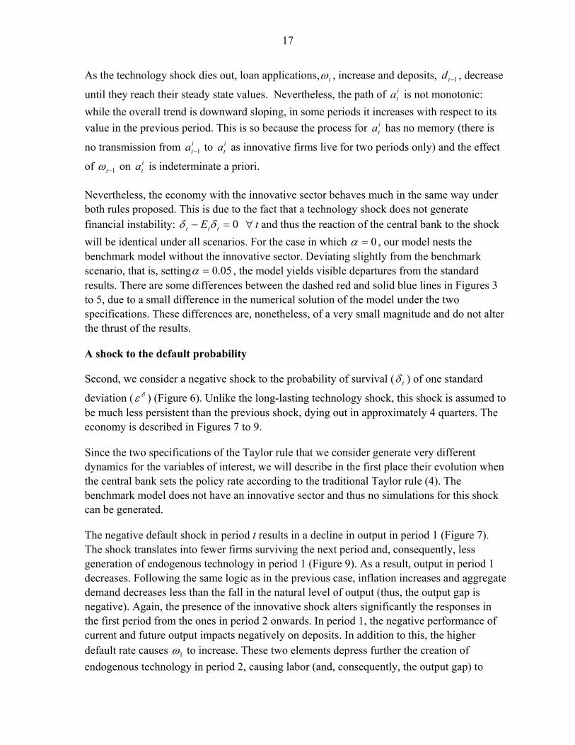
The negative default shock in period t results in a decline in output in period 1 (Figure 7). The shock translates into fewer firms surviving the next period and, consequently, less generation of endogenous technology in period 1 (Figure 9). As a result, output in period 1 decreases. Following the same logic as in the previous case, inflation increases and aggregate demand decreases less than the fall in the natural level of output (thus, the output gap is negative). Again, the presence of the innovative shock alters significantly the responses in the first period from the ones in period 2 onwards. In period 1, the negative performance of current and future output impacts negatively on deposits. In addition to this, the higher default rate causes 1ω to increase. These two elements depress further the creation of endogenous technology in period 2, causing labor (and, consequently, the output gap) to
18
increase even above its steady state level. From period 2 onwards the dynamics of the variables are similar to what is obtained in the benchmark model for a negative technology shock.
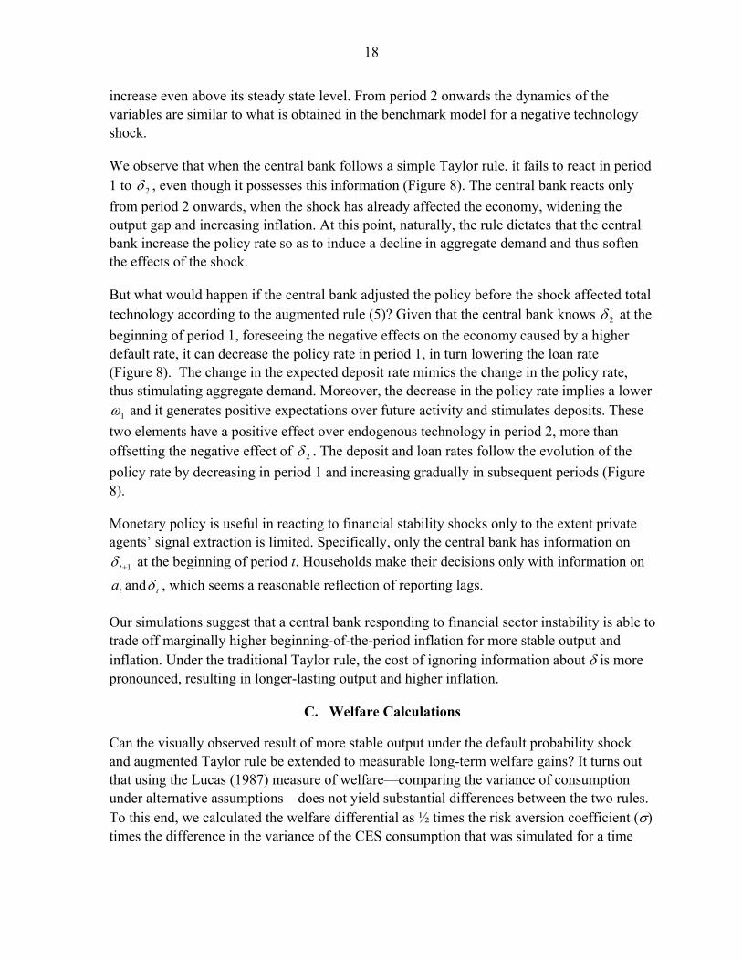
We observe that when the central bank follows a simple Taylor rule, it fails to react in period 1 to 2δ , even though it possesses this information (Figure 8). The central bank reacts only from period 2 onwards, when the shock has already affected the economy, widening the output gap and increasing inflation. At this point, naturally, the rule dictates that the central bank increase the policy rate so as to induce a decline in aggregate demand and thus soften the effects of the shock.
But what would happen if the central bank adjusted the policy before the shock affected total technology according to the augmented rule (5)? Given that the central bank knows 2δ at the beginning of period 1, foreseeing the negative effects on the economy caused by a higher default rate, it can decrease the policy rate in period 1, in turn lowering the loan rate (Figure 8). The change in the expected deposit rate mimics the change in the policy rate, thus stimulating aggregate demand. Moreover, the decrease in the policy rate implies a lower
1ω and it generates positive expectations over future activity and stimulates deposits. These two elements have a positive effect over endogenous technology in period 2, more than offsetting the negative effect of 2δ . The deposit and loan rates follow the evolution of the policy rate by decreasing in period 1 and increasing gradually in subsequent periods (Figure 8).
Monetary policy is useful in reacting to financial stability shocks only to the extent private agents’ signal extraction is limited. Specifically, only the central bank has information on
1+tδ at the beginning of period t. Households make their decisions only with information on
ta and tδ , which seems a reasonable reflection of reporting lags.
Our simulations suggest that a central bank responding to financial sector instability is able to trade off marginally higher beginning-of-the-period inflation for more stable output and inflation. Under the traditional Taylor rule, the cost of ignoring information about δ is more pronounced, resulting in longer-lasting output and higher inflation.
C. Welfare Calculations
Can the visually observed result of more stable output under the default probability shock and augmented Taylor rule be extended to measurable long-term welfare gains? It turns out that using the Lucas (1987) measure of welfare—comparing the variance of consumption under alternative assumptions—does not yield substantial differences between the two rules. To this end, we calculated the welfare differential as ½ times the risk aversion coefficient (σ) times the difference in the variance of the CES consumption that was simulated for a time

19
span of 300 periods (exposing technology and default probability to a simultaneous shock) and repeated 100 times.
The estimates of standard deviations of consumption are practically identical for both rules, and these results are robust with respect to the weight of financial instability in the policy rule ( )δφ . For example, assuming the benchmark value, δφ = –0.5, the standard deviations of consumption under the traditional and augmented rules are virtually identical at 0.05915 and 0.05947, respectively. For a less aggressive rule, δφ = –0.1, the standard deviations are 0.05899 and 0.05892, respectively. Neither of these differences is substantial, meaning that the impact of the augmented rule clearly does not extend into more stable consumption.
These results capture the fact that the economy stabilizes faster under the augmented Taylor rule, but the output and consumption paths are more volatile initially than under the traditional rule. Indeed, in Figure 7, we observe much larger initial, two-period departures from the trend in both output and output gap simulations under the augmented rule than under the traditional rule. In other words, the central bank trades off more instability today for a faster return to the trend path tomorrow. Introduction of the financial sector and shocks thereto in the DSGE model does not change the nature of monetary policy; it only accelerates policy reaction to the signs of financial instability.
V. PRACTICAL ISSUES AND POSSIBLE EXTENSIONS
We see several practical limitations for embracing financial instability as a regular part of a policy rule, namely the magnitude and nature of the initial shock, fiscal repercussions, and exchange rate stability. Finally, we discuss the assumption of central banks’ privileged information and some practical issues and suggestions for further research.
Practical limitations
In the existing model, central bank response to financial instability is linear (as is the simple Taylor rule). In practice, the response is likely to be highly nonlinear: in their reports on financial stability, central banks claim to focus much more on shocks with systemic implications than on smaller shocks with no or limited systemic implications (see, for example, the survey in Čihák, 2006). The long-term fiscal effects of neglected financial instability can be dire. By providing additional liquidity, as opposed to closing down weak financial institutions, the central bank may delay the necessary adjustment and increase the fiscal cost of the eventual cleanup operation. Also, if the financial system is faced with a credibility crisis, a lower policy rate is unlikely to calm the depositors. Monetary easing cannot be a substitute for prudential regulation of the financial system.
The model can be enhanced by introducing other sectors, such as the external sector. Introducing the external sector requires distinguishing residents and nonresidents, and it introduces a role for the exchange rate regime. The scope for monetary easing is more limited
20
in a monetary regime with an exchange rate anchor or with a strong exchange rate transmission channel of monetary policy. Even small monetary easing may cause a run on the currency and force unwinding of external positions. One can expect much less enthusiasm for monetary easing in the face of financial instability in countries with significant capital flows.
The model as presented here focuses only on monetary policy reasons for reactions to financial instability. The central bank in the model responds to financial sector instability not because financial sector developments would have a direct place in its utility function, but simply because responding this way improves developments in future inflation and output. However, there may be other reasons for real central banks to react to instability that are not modeled here. In particular, many central banks have a role in prudential supervision of banks (and sometimes also other financial institutions), and may be perceived responsible for the soundness of the supervised institutions, including ensuring the smooth functioning of the payment and settlement systems, thus putting an even higher premium on financial sector stability. This may create an additional incentive for central banks to lower interest rates to alleviate financial instability. Such central banks also have at their disposal more direct measures of a regulatory or supervisory nature (e.g., they can impose limits on various financial ratios, or demand corrective action from banks’ management). However, those tend to take a longer time and may be more difficult to implement than changes in interest rates.
Privileged information
The simulations suggest that if a central bank has privileged information about the soundness of the financial sector, the information can be used for monetary policy purposes to stabilize output in the face of financial instability shocks. The assumption that central banks have access to privileged information is realistic: central banks usually play an important role in their country’s payment and settlement systems, and many are also prudential supervisors of banks (and in some cases other financial institutions). While individual financial institutions would usually have relatively better information than anybody else (including the central bank) about their own financial health and the financial health of their clients, they would normally not have such information about the other financial institutions in the system, and therefore about the system as a whole. In contrast, the central bank’s unique role in the payment system (and often also in prudential supervision) allows it to have privileged information about financial health on the systemic level.
An interesting question not directly addressed in our model is the central bank’s policy choice regarding the extent to which this privileged information should be revealed to the public. In our model, the public can only extract parts of the central bank’s privileged information from the policy rates. However, a central bank can of course decide to forgo a part of its information superiority, and become more transparent in its assessment of the financial sector, thereby allowing better signal extraction. Indeed, a number of central banks have tried in recent years to increase the amount of information they share about their
21
assessment of financial sector soundness through financial stability reports and other avenues. Some of these central banks have argued that the purpose of these publications is to influence market participants’ decisions and ultimately increase financial stability (e.g., Čihák, 2006).
The willingness and ability of central banks to communicate privileged information to the public may be limited, for several reasons. Some of these are purely legal: banking confidentiality laws in most countries completely prohibit important types of information (e.g., on performance of individual loans) from being distributed to the public. Others are policy-related: sharing information may in some cases trigger the very crisis the central bank is trying to prevent. Whatever the reasons for limiting the amount of information made public, it needs to be stressed that, reflecting these limitations, there are substantial gaps between what some central banks publish in their financial stability reports and what can be considered “good practice” (Čihák, 2006). The central banks’ choice regarding the extent of public access to financial sector information is an interesting issue that could be investigated more in further research.
VI. CONCLUSIONS
Financial instability deserves to be taken seriously because of its macroeconomic costs, but the literature on monetary policy response functions has largely ignored its impact on the behavior of the central bank, basing the policy rule only on the contemporaneous output gap and inflation. To this end, we (i) enrich the standard new Keynesian model with a financial system and firms that require external financing, and (ii) introduce a forward-looking element into the Taylor rule. Under the augmented policy rule the central bank monitors the financial system, responding to deterioration in the financial system balance sheet with instant monetary loosening. Our paper is the first one to model the central bank response to financial instability in a general equilibrium context.
The model fits the stylized facts of modern central banking particularly well. Namely, we know that central banks spend much of their resources on monitoring the economy and financial system, collecting private information that would allow them to respond to forthcoming financial instability shocks well before these shocks are transmitted into headline inflation, output, or other macroeconomic aggregates. The underlying financial shock and its transmission mechanism are integrated into the model, rather than being ad hoc as in the earlier literature.
We find that a policy rule, whereby a central bank lowers its policy rate in response to financial sector instability, yields different short-term outcomes in terms of output and inflation than the traditional Taylor rule. Our model illustrates that as long as the financial instability shock is short-lived and of reasonable magnitude, a forward-looking central bank can prop up the banking system with monetary easing, limiting the short-term fall in the level of output and consumption as compared to the traditional Taylor rule. The central bank
22
following the augmented rule trades off more output and inflation instability today for a faster return to the trend path tomorrow. The nature of monetary policy remains unchanged under this rule, and although the reaction of the central bank to financial instability is much faster than under the Taylor rule, the long-run impact on consumption appears negligible.
23
REFERENCES
Berger, Allen, Sally Davies, and Mark Flannery, 2001, “Comparing Market and Supervisory Assessments of Bank Performance: Who Knows What and When?” Journal of Money Credit and Banking, 32, pp. 641–667.
Bernanke, Ben, and Mark Gertler, 1999, “Monetary policy and asset price volatility”, Economic Review (Kansas City: FRB of Kansas City), 4th quarter, pp. 17–51. Available via the internet: http://www.kc.frb.org/PUBLICAT/ECONREV/PDF/4q99bern.pdf.
Bernanke, Ben, Mark Gertler, and Simon Gilchrist, 1998, “The Financial Accelerator in a Quantitative Business Cycle Framework,” NBER Working Paper No. 6455 (Cambridge, Massachusetts: National Bureau of Economic Research). Available via the internet: http://www.nber.org/papers/w6455.pdf.
Bongini, Paola, Luc Laeven, and Giovanni Majnoni, 2002, “How Good Is the Market at Assessing Bank Fragility? A Horse Race between Different Indicators”, Journal of Banking and Finance, Vol. 26, No. 5 (May 2002), pp. 1011–28.
Bordo, Michael D., Olivier Jeanne, 2002, “Boom-Busts in Asset Prices, Economic Instability, and Monetary Policy,” NBER Working Paper No. 8966 (Cambridge, Massachusetts: National Bureau of Economic Research). Available via the internet: http://www.nber.org/papers/w8966.
Borio, Claudio, 2006, “Monetary and Prudential Policies at a Crossroads? New Challenges in the New Century,“ BIS Working Papers No. 216 (Basel: Bank for International Settlements). Available via the internet: http://www.bis.org/publ/work216.pdf.
Borio, Claudio, and Philip Lowe, 2004, “Securing Sustainable Price Stability: Should Credit Come Back from the Wilderness?” BIS Working Papers No. 157 (Basel: Bank for International Settlements). Available via the internet: http://www.bis.org/publ/work157.pdf.
Borio, Claudio, and William R. White, 2003, “Wither Monetary and Financial Stability? The Implications of Evolving Policy Regimes,” in Monetary Policy and Uncertainty: Adapting to a Changing Economy, A symposium sponsored by the Federal Reserve Bank of Kansas City, Jackson Hole, Wyoming, August 28-30, 2003. Available via the internet: http://www.kc.frb.org/PUBLICAT/SYMPOS/2003/pdf/Boriowhite2003.pdf.
Boorman, Jack, Timothy D. Lane, Marianne Schulze-Ghattas, Aleš Bulíř, Atish R. Ghosh, A. Javier Hamann, 2000, “Managing Financial Crises: The Experience in East Asia,” Carnegie-Rochester Conference Series on Public Policy, Vol. 53 (December), pp. 1-67.
24
Brousseau, Vincent, and Carsten Detken, 2001, “Monetary Policy and Fears of Financial Instability,” ECB Working Paper Series, No. 89 (Frankfurt: European Central Bank). Available via the internet: http://www.ecb.int/pub/pdf/scpwps/ecbwp089.pdf.
Bulíř, Aleš, and Martin Čihák, 2007, “Central Bankers’ Dilemma When Banks Are Fragile: To Tighten or not to Tighten?” International Monetary Fund, mimeo.
Calvo, Guillermo A., 1983, “Staggered Prices in a Utility-Maximizing Framework,” Journal of Monetary Economics, Vol. 12 (September), pp. 383–98.
Cecchetti, Stephen, Hans Genberg, John Lipsky, and Sushil Wadhwani, 2000, “Asset Prices and Central Bank Policy,” ICMB/CEPR Report, No. 2 (London: Centre for Economic Policy Research).
Cecchetti, Stephen, and Lianfa Li, 2005, “Do Capital Adequacy Requirements Matter for Monetary Policy?” NBER Working Paper No. 11830 (Cambridge, Massachusetts: National Bureau of Economic Research). Available via the internet: http://www.nber.org/papers/w11830.
Čihák, Martin, 2006, “How Do Central Banks Write on Financial Stability?” IMF Working Paper 06/163 (Washington: International Monetary Fund). Available via the internet: http://www.imf.org/external/pubs/ft/wp/2006/wp06163.pdf.
Crockett, Andrew, 1997, “Why is Financial Stability a Goal of Public Policy?” in Maintaining Financial Stability in a Global Economy, A symposium sponsored by the Federal Reserve Bank of Kansas City, Jackson Hole, Wyoming, August 28-30, 1997. Available via the internet: http://www.kc.frb.org/publicat/econrev/pdf/4q97croc.pdf.
Fukač, Martin, and Adrian Pagan, 2006, “Issues in Adopting DSGE Models for Use in the Policy Process,” CNB WP No. 5/2006 (Czech National Bank: Prague). Available via the internet: http://www.cnb.cz/www.cnb.cz/en/research/research_publications/cnb_wp/download/cnbwp_2006_06.pdf.
Galí, Jordi, 2002, “New Perspectives on Monetary Policy, Inflation, and the Business Cycle,” NBER Working Paper No. 8767 (Cambridge, Massachusetts: National Bureau of Economic Research). Available via the internet: http://www.nber.org/papers/w8767.
Henry, Peter Blair, 2004, “Financial Instability: Perspective Paper,” in Bjørn Lomborg, ed., Global Crises, Global Solutions (Cambridge, New York, and Melbourne: Cambridge University Press).
Lucas, Robert, 1987, Models of Business Cycles, (New York: Basil Blackwell).
25
Monacelli, Tommaso, 2004, “A Dynamic Optimizing New Keynesian Framework for Monetary Policy Analysis,” mimeo, IGIER. Available via the internet: http://www.igier.uni-bocconi.it/whos.php?vedi=1830&tbn=albero&id_doc=177.
Quintyn, Marc, Silvia Ramirez , Michael W. Taylor, 2007, “The Fear of Freedom: Politicians and the Independence and Accountability of Financial Sector Supervisors,” IMF Working Paper 07/25 (Washington: International Monetary Fund). Available via the internet: http://www.imf.org/external/pubs/ft/wp/2007/wp0725.pdf.
Schwartz, Anna, 1995, "Why Financial Stability Depends on Price Stability", Economic Affairs, Vol. 15 (Autumn), pp. 21–25.
Svensson, Lars E. O., 2003, “What Is Wrong with Taylor Rules? Using Judgment in Monetary Policy through Targeting Rules,” Journal of Economic Literature, Vol. 41 (June), pp. 426–77.
Taylor, John B., 1993, “Discretion Versus Policy Rules in Practice,” Carnegie-Rochester Conference Series on Public Policy, Vol. 39, December, pp. 195–214.
Williamson, Stephen D., 1987, “Financial Intermediation, Business Failures, and Real Business Cycles,” The Journal of Political Economy, Vol. 95 (December), pp. 1196--216.
26
APPENDIX
To derive the equations to solve the model numerically we follow Monacelli (2004).
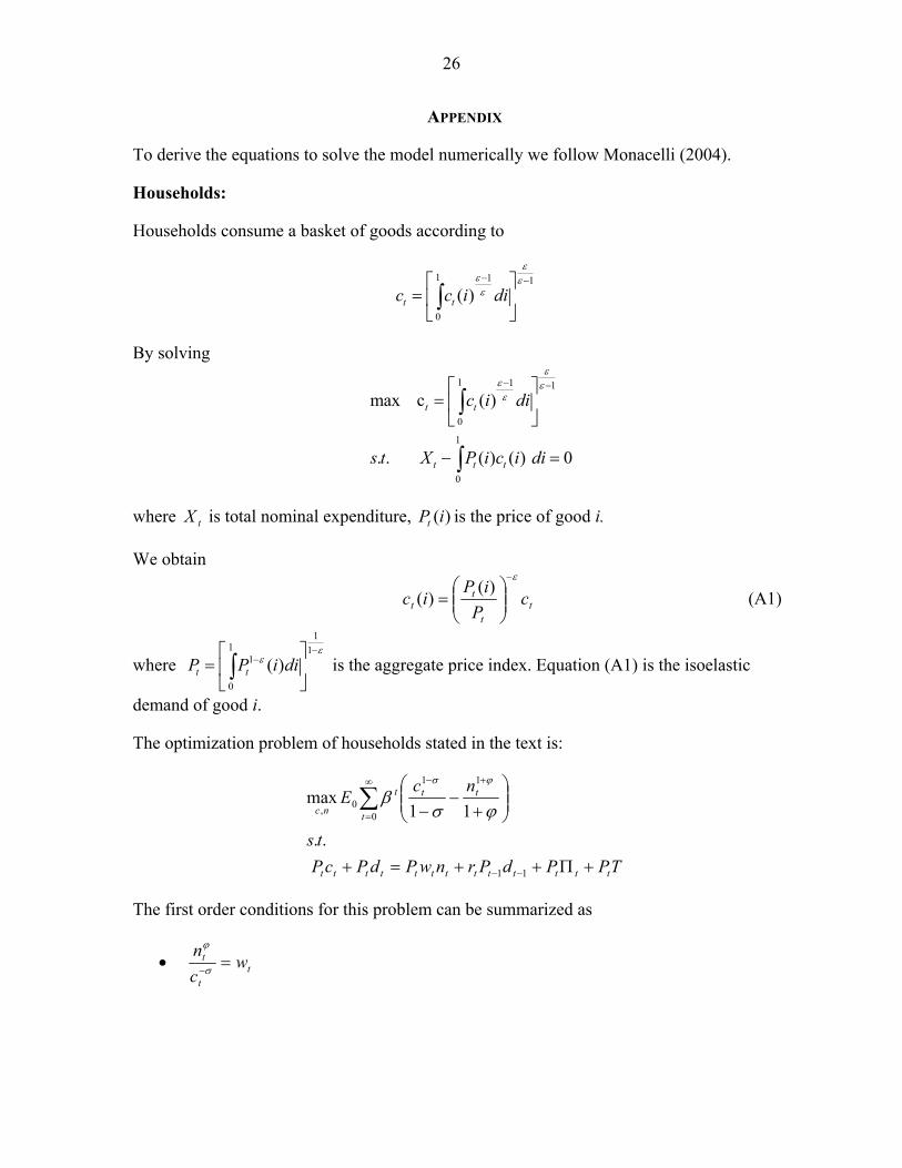
Households:
Households consume a basket of goods according to
1 1 1
0
( )t tc c i di
εε εε− −⎡ ⎤
= ⎢ ⎥⎣ ⎦∫
By solving 1 1 1
0
1
0
max c ( )
. . ( ) ( ) 0
t t
t t t
c i di
s t X P i c i di
εε εε− −⎡ ⎤
= ⎢ ⎥⎣ ⎦
− =
∫
∫
where tX is total nominal expenditure, )(iPt is the price of good i.
We obtain
tt
tt c
PiP
icε−
⎟⎟⎠
⎞⎜⎜⎝
⎛=
)()( (A1)
where
11 1
1
0
( )t tP P i diε
ε−
−⎡ ⎤= ⎢ ⎥⎣ ⎦∫ is the aggregate price index. Equation (A1) is the isoelastic
demand of good i.
The optimization problem of households stated in the text is:
TPPdPrnwPdPcPts
ncE
ttttttttttttt
t
ttt
nc
+Π++=+
⎟⎟⎠
⎞⎜⎜⎝
⎛+
−−
−−
∞
=
+−
∑
11
0
11
0,
..
11max
ϕσβ
ϕσ
The first order conditions for this problem can be summarized as
• tt
t wcn
=−σ
ϕ
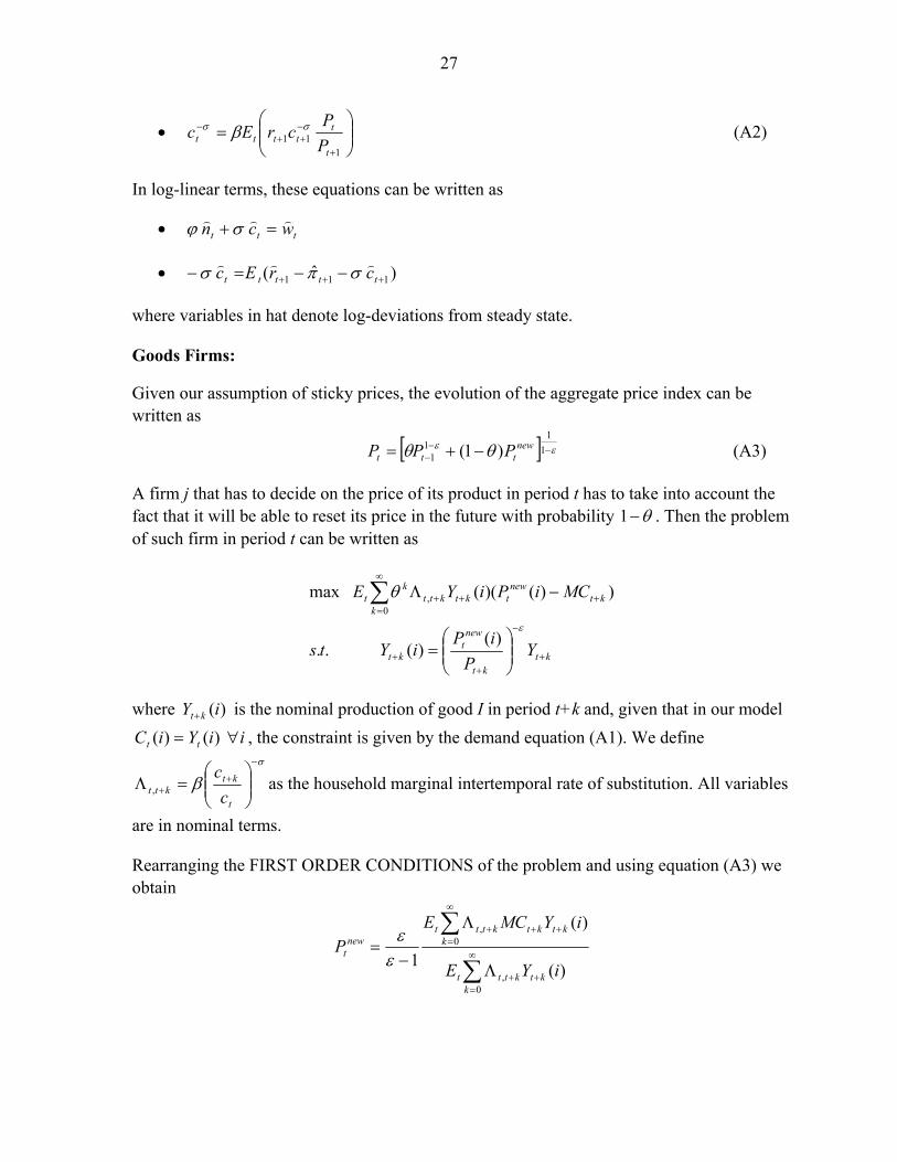
27
• ⎟⎟⎠
⎞⎜⎜⎝
⎛=
+
−++
−
111
t
ttttt P
PcrEc σσ β (A2)
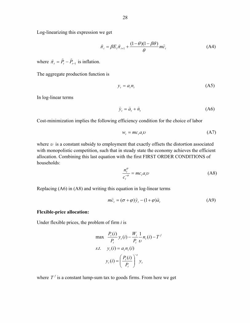
In log-linear terms, these equations can be written as
• ttt wcn ))) =+ σϕ
• ) ˆ( 111 +++ −−=− ttttt crEc ))) σπσ
where variables in hat denote log-deviations from steady state.
Goods Firms:
Given our assumption of sticky prices, the evolution of the aggregate price index can be written as
[ ] εε θθ −−− −+= 1
11
1 )1( newttt PPP (A3)
A firm j that has to decide on the price of its product in period t has to take into account the fact that it will be able to reset its price in the future with probability θ−1 . Then the problem of such firm in period t can be written as
ktkt
newt
kt
kkt
newtktktt
kt
YP
iPiYts
MCiPiYE
+
−
++
∞
=+++
⎟⎟⎠
⎞⎜⎜⎝
⎛=
−Λ∑ε
θ
)()( ..
))()(( max0
,
where )(iY kt+ is the nominal production of good I in period t+k and, given that in our model iiYiC tt ∀= )()( , the constraint is given by the demand equation (A1). We define
σ
β−
++ ⎟⎟
⎠
⎞⎜⎜⎝
⎛=Λ
t
ktktt c
c, as the household marginal intertemporal rate of substitution. All variables
are in nominal terms.
Rearranging the FIRST ORDER CONDITIONS of the problem and using equation (A3) we obtain
∑
∑∞
=++
∞
=+++
Λ
Λ
−=
0,
0,
)(
)(
1k
ktkttt
kktktkttt
newt
iYE
iYMCEP
εε
28
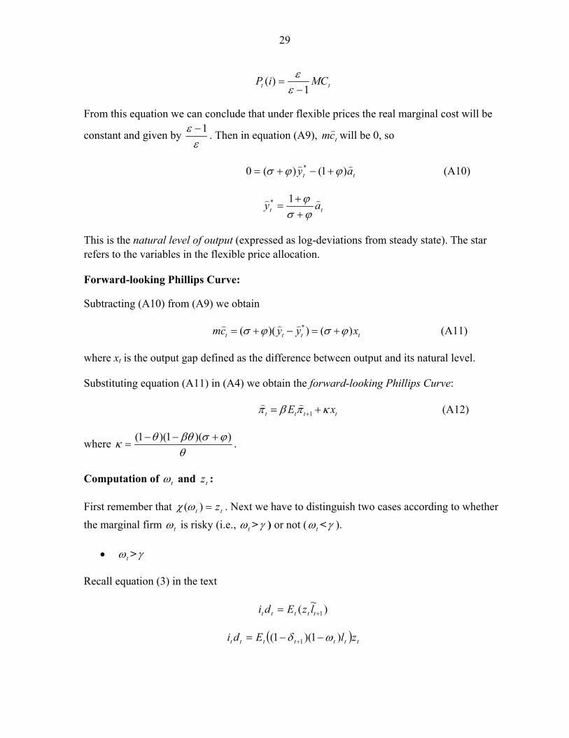
Log-linearizing this expression we get
tttt cmE )))
θβθθπβπ )1)(1(
1−−
+= + (A4)
where 1−−= ttt PP)))π is inflation.
The aggregate production function is
ttt nay = (A5)
In log-linear terms
ttt nay ))) += (A6)
Cost-minimization implies the following efficiency condition for the choice of labor
υttt amcw = (A7)
where υ is a constant subsidy to employment that exactly offsets the distortion associated with monopolistic competition, such that in steady state the economy achieves the efficient allocation. Combining this last equation with the first FIRST ORDER CONDITIONS of households:
υσ
ϕ
ttt
t amccn
=− (A8)
Replacing (A6) in (A8) and writing this equation in log-linear terms
ttt aycm ))) )1()( ϕϕσ +−+= (A9)
Flexible-price allocation:
Under flexible prices, the problem of firm i is
tt
tt
ttt
ft
t
tt
t
t
yP
iPiy
inaiyts
TinPW
iyP
iP
ε
υ
−
⎟⎟⎠
⎞⎜⎜⎝
⎛=
=
−−
)()(
)()( ..
)(1)()(
max
where fT is a constant lump-sum tax to goods firms. From here we get
29
tt MCiP1
)(−
=εε
From this equation we can conclude that under flexible prices the real marginal cost will be
constant and given by ε
ε 1− . Then in equation (A9), tcm) will be 0, so
tt ay )) )1()(0 * ϕϕσ +−+= (A10)
tt ay ))
ϕσϕ++
=1*
This is the natural level of output (expressed as log-deviations from steady state). The star refers to the variables in the flexible price allocation.
Forward-looking Phillips Curve:
Subtracting (A10) from (A9) we obtain
*( )( ) ( )t t t tmc y y xσ ϕ σ ϕ= + − = +) ) ) (A11)
where xt is the output gap defined as the difference between output and its natural level.
Substituting equation (A11) in (A4) we obtain the forward-looking Phillips Curve:
1t t t tE xπ β π κ+= +) ) (A12)
where θ
ϕσβθθκ ))(1)(1( +−−= .
Computation of tω and tz :
First remember that tt z=)(ωχ . Next we have to distinguish two cases according to whether the marginal firm tω is risky (i.e., tω >γ ) or not ( tω <γ ).
• tω >γ
Recall equation (3) in the text
)~( 1+= ttttt lzEdi
( ) ttttttt zlEdi )1)(1( 1 ωδ −−= +
30
)1()( 1+−= tttt Ei δωχ
Then tω can be computed as the cdf of a lognormal distribution with parameters μ and σ
for )1( 1+− tt
t
Eiδ
.
• tω <γ
Again, taking into account that )~( 1+= ttttt lzEdi
tttttttt zllEdi⎟⎟⎟⎟
⎠
⎞
⎜⎜⎜⎜
⎝
⎛
−−+−= + )1()1()( 1
loansfor ask thatfirmsrisky
loansfor ask that firmsrisky -non
δγωγ32143421
In this case tω needs to be computed by a numerical root-finding algorithm.
Let Atz be the loan rate that is charged when tω <γ and B
tz the one charged when tω >γ . Then for a given ti ,:
t
ttttt
tttttt
tttt
EE
EEE
ωδγωγ
δ
δγωγωδωγωγδ
−−−+−
<−⇒
−−+−<−−⇒−<−−
++
++
+
1)1()1()(
)1(
)1()1()()1)(1()())(1(
11
11
1
So it follows that Bt
At zz < .
Steady State: First notice that in steady state 11 =⇒== aaa si 7. Then ncy == .
7 In order to have ia we normalize it so that ( )11 1
*
1
)()(1 −−
⎥⎥⎦
⎤
⎢⎢⎣
⎡= ∫
−
ττ
ω
ττ
δ djjjsA
at
ttiit , where
( ) 11 1* )()(
−−
⎥⎦
⎤⎢⎣
⎡= ∫
ττ
ω
ττ
δ djjjsAi and ω and *δ are steady state values.
31
From equation (A2) we can see that in steady state
β1
=R
From the first condition of the household optimization problem, we can conclude that
wy =+σϕ . It can be shown that in order to attain the efficient allocation, 1−
=εευ . Also,
εε 1−
=mc . From equation (A7) we find then that 11 ===⇒= ncyw .
Finally, we assume 1=P , so the budget constraint of households is
TdRnwdc −Π++=+ **
First notice that in steady state
f
f
T
Tnwy
−−=Π
−−=Π
υ
υ11
*1
We will assume that fT is such that ε10 =⇒=Π fT
Given that in steady state the government has a balanced budget, we know that
)1(1)1(
1 −+−
=⇒−
=+=εε
εεεευ TTT f .
We will assume that, unlike profits Π , lump-sum taxes to households are constant every period. Then substituting in the period-by-period budget constraint of households, we find that deposits in steady state are
0)1(
1)1(1
1>
−−−
−=
εεεε
Rd because 1 ,0)1( ><− εR
Computation of deposits:
Combining the period-by-period budget constraint of households and the Euler Equation (A2) we can write
t
ttttttttt
t
t
t
ttt P
PdrTnwdr
PP
cc
Ec 111
1
1 −−+
+−
−+ =+Π−−+ σ
σ
β (A13)
32
Iterating forward and using the transversality condition 0lim 11
1
=−+++
−+−
−+
−+
∞→ jtjtjt
jt
jt
jtj
jdr
PP
ccσ
σ
β we
obtain:
( )∑∞
=+++++−
−+
−− +Π−−=
01
1
jjtjtjtjtjt
t
jtjtt
t
tt Tnwc
cc
EdP
Pr σ
σ
β (A14)
Log-linearizing equation (A13) we obtain
( )( )
11
111
ˆˆˆˆˆ
ˆˆ)ˆˆ(ˆˆ)(
ˆˆˆˆˆ
−−−−
−−−
−−
−+
−+
−−+
−
++−+−
=+ΠΠ−+−++Π−−−
++−+−
ttttt
tttttt
tttttt
dRDCrRDCpRDCpRDCcRDC
tTnwWNcCCcTWNCC
dRDCrRDCpRDCpRDCcRDCE
σσσσσ
σσ
σσσσσ
σ
σ
σβ
As we have shown before, in steady state we have that ,1=== WNC and 0=Π . Since taxes are constant, 0ˆ =tt . Finally, given our parameterization, .1=σ The latter expression becomes
( ) )ˆˆˆ(ˆ)ˆˆ(ˆ)1()ˆˆˆ(ˆ 1111 tttttttttttt drRDcRDnwcTdrRDcRDE ππβ −++−=+−−+−++− −+++
This can be re-written as
)()ˆˆ(ˆ)1()( 1+++−−= tttttt sVEnwcTsV β
where )ˆˆˆ(ˆ)( 1 ttttt drRDcRDsV π−++−= − . Imposing the transversality condition, it is easy to see that this is a contraction. Then we can solve for )( tsV by value function iteration. Now
we need to extract td̂ from this expression. Log-linearizing expression (A2) and imposing the conditions of steady state as before we obtain
)ˆˆˆ(ˆˆˆˆ 1 ttttttt drRDnwdDc π−+++=+ −
Adding and subtracting tcRD ˆ from the previous expression we obtain td̂
( ))(ˆ)1(ˆˆ1ˆttttt sVcRDnw
Dd +−++=
Equations (A6), (A7) in log-linear terms, (A11) and (A12) are, together with the two first order conditions for households, the equations corresponding to the innovative firms and financial intermediaries stated in the text and the expression for deposits, the fundamental equations of the model.
33
Figure 1: Distribution of Returns of Innovative Firms
34
Figure 2. Shock to Exogenous Technology (One standard deviation of the technology shock, aε )
35
Figure 3. Shock to Exogenous Technology: Response of Output, Output Gap, Inflation, and Labor
(One standard deviation of the technology shock, aε )
36
Figure 4. Shock to Exogenous Technology: Response of Policy Rate, Real Interest Rate, Loan Rate, and Effective Deposit Rate
(One standard deviation of the technology shock, aε )
37
Figure 5. Shock to Exogenous Technology: Response of tω , Endogenous Technology and Total Technology
(One standard deviation of the technology shock, aε )
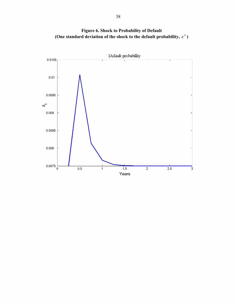
38
Figure 6. Shock to Probability of Default (One standard deviation of the shock to the default probability, δε )
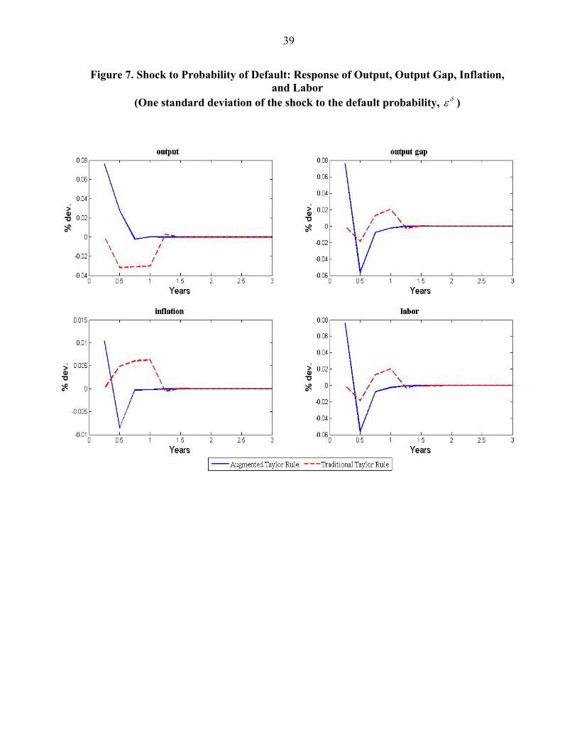
39
Figure 7. Shock to Probability of Default: Response of Output, Output Gap, Inflation, and Labor
(One standard deviation of the shock to the default probability, δε )

40
Figure 8. Shock to Probability of Default: Response of Policy Rate, Real Interest Rate, Loan Rate, and Effective Deposit Rate
(One standard deviation of the shock to the default probability, δε )
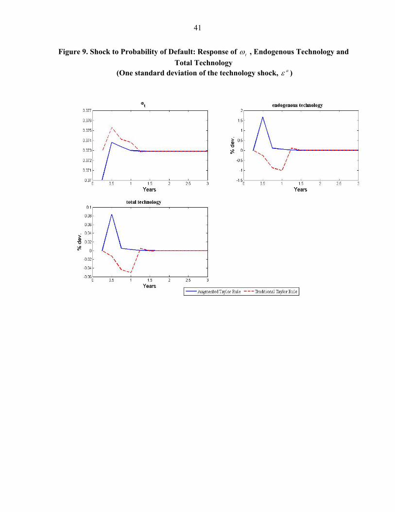
41
Figure 9. Shock to Probability of Default: Response of tω , Endogenous Technology and Total Technology
(One standard deviation of the technology shock, aε )