tcp over cdma2000 networks: a cross-layer measurement · pdf filetcp over cdma2000 networks :...

TECHNICAL REPORT BUCS-TR-2006-030. SPRINT TECHNICAL REPORT RR06-ATL-101579. 1

TCP over CDMA2000 Networks : A Cross-LayerMeasurement Study

Karim Mattar∗ Ashwin Sridharan† Hui Zang† Ibrahim Matta∗ Azer Bestavros∗

∗Computer Science Dept., Boston University, Boston, MA{kmattar, matta, best}@cs.bu.edu

†IP and Wireless Research Group, Sprint ATL, Burlingame, CA{ashwin.sridharan, hui.zang}@sprint.com

Technical Report BUCS-TR-2006-030

Sprint Technical Report RR06-ATL-101579

Abstract

Modern cellular channels in 3G networks incorporate sophisticated power control and dynamic rate adaptationwhich can have significant impact on adaptive transport layer protocols, such as TCP. Though there exists studiesthat have evaluated the performance of TCP over such networks, they are based solely on observations at thetransport layer and hence have no visibility into the impact of lower layer dynamics, which are a key characteristicof these networks. In this work, we present a detailed characterization of TCP behavior based on cross-layermeasurement of transport layer, as well as RF and MAC layer parameters. In particular, through a series of activeTCP/UDP experiments and measurement of the relevant variables at all three layers, we characterize both, thewireless scheduler and the radio link protocol in a commercial CDMA2000 network and assess their impact onTCP dynamics. Somewhat surprisingly, our findings indicate that the wireless scheduler is mostly insensitive tochannel quality and sector load over short timescales and is mainly affected by the transport layer data rate.Furthermore, with the help of a robust correlation measure, Normalized Mutual Information, we were able toquantify the impact of the wireless scheduler and the radio link protocol on various TCP parameters such as theround trip time, throughput and packet loss rate.

I. INTRODUCTION

With advances in error-correction coding, processing power and cellular technology, the wireless channelneed no longer be viewed as an error-prone channel with low bandwidth. Instead, modern 3G cellularnetworks (e.g CDMA2000 1xRTT, EV-DO[18], HSDPA/UMTS) deploy ARQ mechanisms for fast errorrecovery, as well as sophisticated wireless schedulers that can perform “on-the-fly” rate adaptation. Thelatter feature allows the network to adapt to diverse conditions such as poor channel quality, sector loadand more importantly, as we show in this work, data backlog in the user buffer.

The dynamic rate adaptation of modern cellular channels implies that a source will typically experiencevariable bandwidth and delay, which may be caused by the scheduler’s dependency on buffer backlog.Since TCP, the dominant transport protocol in the Internet, utilizes feedback from the channel to controlits transmission rate (indirectly the buffer backlog), this creates a situation where two controllers, thewireless scheduler and TCP, share a single control variable.

There are several interesting studies that have considered the performance of TCP over cellular networks([15], [5], [20]). However, they mostly rely on measurement of TCP dynamics at the transport layer andhave no visibility into the underlying MAC nor the dynamics of the radio channel. In this work, wemeasure relevant information at all three layers in a commercial CDMA2000 network to identify thedominant factors that affect TCP. To the best of our knowledge, this is the first study that looks atcross-layer measurements in a wireless network.


Our contributions can be summarized as follows:1) We conducted extensive active measurements in a commercial CDMA2000 cellular network to

characterize the behavior of the wireless scheduler, and evaluate TCP’s performance. One of ourobjectives was to identify the impact of various network factors on both the wireless scheduler andTCP. Towards this end, we develop a simple Information Theoretic framework that allows us toquantify how factors such as channel quality, sector load etc., affect the wireless scheduler, and howthe scheduler in turn affects TCP.

2) In terms of the wireless scheduler, we exposed the different mechanisms that govern its operation andidentified the characteristics that influence its performance. We concluded that over short timescales(1 second), the channel rate scheduler : a) is highly dependent on buffer backlog, b) is surprisinglyinsensitive to variations in channel quality or sector load, c) has a rate limiting mechanism tomaintain fairness by throttling connections that are being persistently greedy. Over long timescales(20 minutes), however, the scheduler reduces allocated rate in response to persistently bad channelconditions or high sector load and is unable to maintain fairness among concurrent TCP sessions,and d) performs poorly when traffic sources are more aggressive in acquiring bandwidth.

3) In terms of the radio link protocol, we show that a high frame loss (or error) rate could be due to acongested back-haul link that causes packets to get lost (or corrupted) after they are broken downinto frames by the Base Station Controller.

4) In terms of TCP, we concluded that : a) there is a tight coupling between the TCP sending rateand the wireless scheduler. This implies that rate variations, seen by TCP, on the CDMA channelare not random, b) congestion induced losses are more prevalent than wireless losses, c) the highvariability in channel rate causes frequent timeouts which can be alleviated by using the time-stampoption and d) the radio link protocol, despite employing an aggressive retransmission scheme tosignificantly reduce wireless losses, has a limited impact on TCP’s round trip time and throughput.

5) Finally, as a general observation, we found high variability in TCP throughput based on the timeand day of the experiment. We hypothesize this to be due to rapid cell dimensioning by networkoperators.

The rest of the paper is organized as follows: Section II outlines the architecture of a CDMA2000network and highlights the relevant features. Section III presents a description of the various experi-ments that we conducted. Section IV explains our empirical evaluation methodology which is based oncorrelating time series that capture the evolution of various system parameters, to better understand theinterdependence between different system components. Section V characterizes the wireless schedulerand quantifies the relative impact of various factors on it. Section VII presents an evaluation of TCP’sperformance. Section VIII presents our conclusions.

II. THE CDMA2000 1XRTT SYSTEM

In this section, we illustrate the architecture of modern cellular data networks, as well as identify salientproperties of CDMA2000 1xRTT, a 2.5G technology, which is widely used in these networks and was thetechnology available at the time we conducted our experiments. In particular, we highlight key features ofthe CDMA2000 network, that either directly or indirectly affect higher layer performance and motivate theneed to characterize their impact in realistic environments. We believe our findings may also be applicableto current 3G networks based on the 1xEV-DO technology [18] because they share some similar features.

A. Network Architecture

Figure 1 sketches the architecture of a typical cellular data network. The network consists of two maincomponents: the radio network and the data network. The data network is an all-IP network comprising ofthe PDSN (Packet Data Serving Node), the HA (Home Agent) and the AAA (Authentication, Authorizationand Accounting) server. The PDSN, residing in the data network, acts as the interface agent between thetwo networks. It establishes a PPP session for each cellular user and forwards traffic received from the


Fig. 1. Network Architecture

radio network to the HA and vice versa. The HA is responsible for IP address allocation, forwardingcellular IP traffic to (and from) the Internet and more importantly, manages user mobility via MobileIP [7]. The AAA server mainly addresses the requirements of authentication, billing etc.

The radio network, which is actually the focus of this study, comprises the air interface and two basicelements: a Base Transceiver Station (BTS) and a Base Station Controller (BSC). The BTS, or simply put,the base station, is essentially a “dumb terminal” in the CDMA2000 1xRTT network, comprising onlyof antenna arrays to efficiently radiate RF (Radio Frequency) power to mobile users, as well as receivesignals from them. Hence, it acts as the interface between the “wireline” network and the “wireless”hop. Each such base station represents a “cell”. For purposes of efficient frequency re-use, the cell istypically split into three sectors by suitable alignment of the antenna profile into three geographicallydistinct radiation beam patterns. Users in the same cell but different sectors can operate independently,but users in the same sector must share air resources.

The BSC, which is actually the main element of the radio network, is an intelligent agent that cancontrol up to 400 base stations (or cells) that are connected to it through a low latency back-haul network.The BSC is responsible for almost all the RF layer operations that are critical for the smooth operationof the CDMA network. Among other things, it manages power control operations for all mobile users tolimit interference and also controls soft-handoff [23] as users move.

From the perspective of a transport layer such as TCP, the two most critical actions controlled by theBSC that explicitly affect TCP’s performance are: a) the channel rate allocation on the wireless hop toeach user on both the downlink1 and the uplink and b) the Radio Link Protocol (RLP), which is a linklayer error and loss recovery mechanism.

While various other RF related factors like channel conditions, number of users, channel errors etc.,clearly affect higher layer performance, as explained in later sections, their impact is subsumed in thesetwo functions. In other words, they indirectly affect application performance by either affecting the channelrate or RLP behavior. Consequently, in this work, we view them as secondary factors, while the channelrate and RLP as primary factors that directly affect higher layer performance.

1The downlink is the path from the BSC to the user, while the uplink is the path from the user to the BSC.


B. Wireless Scheduler

Current and next generation cellular data networks possess the ability to dynamically vary the rate of thewireless channel assigned to a user through a combination of adaptive coding, modulation and orthogonalWalsh Codes. Clearly, variation in the assigned channel rate has a direct impact on the throughput perceivedby higher layer protocols.

In a CDMA2000 1xRTT network, this operation is performed by the BSC primarily by changing theWalsh Code. Specifically, the BSC can assign a higher (lower) rate to a mobile by assigning a shorter(longer) Walsh Code. Depending on the Radio Configuration Type [23] a CDMA2000 1xRTT network cansupport up to six different channel rates. The network utilized for our experiments supports five channelrates. The smallest assignable rate, denoted by the Fundamental Channel (FCH) is 9.6 kbps. This is thestandard channel assigned to all voice users and initially to a data user upon joining the network. If auser requires higher data rates, the BSC can assign it a Supplemental Channel (SCH) in bursts of shortdurations. The Supplemental Channel can take rates from the set {19.2,38.4,76.8,153.6} kbps.

Though a shorter Walsh Code increases the data rate, it has two drawbacks. First, the reduced codelength degrades “orthogonality”, which makes the signal more susceptible to interference from other users.To overcome this problem, the BSC employs two techniques:

1) The signal strength is boosted for users assigned a higher rate channel to overcome increasedinterference.

2) When a user is assigned a higher rate channel, fewer users are allowed to simultaneously transmitat high rates to reduce interference. The higher the rate is, the fewer the number of users that canbe assigned this rate simultaneously. In the extreme case, only one user can be assigned the highestrate, 153.6 kbps, at any point in time. Consequently, in order to provide fairness, high rate channelsare allocated only in short bursts.

The BSC may assign a supplemental channel with the appropriate rate to a user based on the followingpotential secondary factors:

• Buffer backlog: The CDMA2000 1xRTT network deploys a per-user buffer at the BSC which isroutinely monitored by the scheduler. A large data backlog is more likely to trigger assignment of ahigh rate Supplemental Channel for the user.

• Channel conditions: Each base station transmits a continuous Pilot Signal which is received by allusers in the cell. The user then determines the channel condition by computing the Pilot SINR Ec/Io,where Ec represents the strength of the Pilot Signal received and Io the interference due to otherusers and thermal noise. A low value indicates poor channel conditions (or high loss) and vice versa2.This value is fed back to the BSC which utilizes this information in deciding what rate to assign. Apoor channel may result in a reduction in the assigned rate to minimize channel losses.

• Sector load (in terms of number of users): As mentioned earlier, shorter Walsh Codes (at the samepower) experience higher interference and also cause more interference. Hence, whenever the BSCtransmits a high rate SCH burst to a user, it may prevent other users from transmitting at high rates.Consequently, the BSC must take into consideration the number of other active users in a sectorbefore determining what rate to assign.

C. Radio Link Protocol

Apart from wireless channel rate allocation, the other feature of the BSC that can directly affect higherlayer performance is the Radio Link Protocol (RLP). The RLP is a NACK-based ARQ re-transmissionmechanism developed in order to minimize the losses perceived by higher layers. The motivation for

2Typical values for good channels are around −3 to −7 dB, while values less than −11dB indicate a poor channel.


such a mechanism is the high latency on wireless links which can induce large delays before end-to-endrecovery mechanisms sense and recover from a packet loss.

The BSC maintains an RLP session with each mobile user which works as follows. The BSC breaksincoming IP packets from the PDSN into radio frames which are then transmitted to the mobile viathe BTS. The mobile, on detecting missing (or corrupted) RLP frames requests re-transmission of thecorresponding RLP frames.

D. Impact of Wireless Scheduler and Radio Link Protocol on TCP

It has been traditionally assumed that the RLP re-transmission rate is closely related to the Frame ErrorRate (FER) of the channel. In this context, the impact of the Radio Link Protocol on TCP has beenextensively researched theoretically [10], [16], [2], [4] from the perspective of trade-off between reducederror probability and increased latency to maximize throughput. The link layer increases the reliability seenby higher layers through re-transmissions or stronger error correcting codes. Both mechanisms attemptto reduce the likelihood of TCP throttling its sending rate due to packet losses. On the other hand, thesemechanisms increase latency since packets are retained longer by the link layer for successful transmission,which in turn can degrade throughput.

To the best of our knowledge, neither the RLP re-transmission rate and its dependence on the channelFER, nor the impact of the link layer on TCP dynamics have been quantified in practice on commercialnetworks. Even less research has been conducted on the impact of dynamic wireless channel rate allocationon TCP performance (see [1], [8] for models) or to which extent each of the secondary factors influencesthe channel assigned rate. The only experimental study we are aware of is the one presented in [9] whichevaluated the impact of bandwidth variation in CDMA2000 networks on the TCP timeout mechanism ina lab environment.

As discussed in Section II-B, the assigned channel rate can be affected by three secondary factors:channel conditions, application data rate and sector load. However, it is not clear in practice which factordominates. If the channel conditions play the dominant role in determining the assigned channel rate, anargument similar to that for RLP could potentially be made in that it, too, trades-off channel bandwidthto minimize channel errors, and thus should have an impact similar to that of RLP.

However, an important difference from RLP is that the data sending rate of the higher layer protocolalso affects the assigned channel rate. This is crucial because, TCP, the most widely used transport layerprotocol, is a reactive protocol which adjusts its rate based on feedback from the receiver. Hence, thesystem becomes a closed-loop system where both TCP and the BSC scheduler vary their rate based onfeedback from the other. This may result in unexpected interactions between the two control regimes,possibly leading to performance degradation.

The objective of this study is to precisely characterize these issues. Through a series of experiments, weevaluate which secondary RF layer factors affect the assigned channel rate and the Radio Link Protocolthe most. We also study the impact of both RLP and the wireless scheduler on TCP dynamics.

III. EXPERIMENTS AND DATA SETS

Our primary focus is the downlink. We therefore performed end-to-end experiments which involved datatransfer via either UDP or TCP SACK from a RedHat Linux server on the Internet to one or more laptopsrunning Windows XP that were connected to the cellular data network via CDMA2000 1xRTT air-cards.A typical experimental setup is shown in Fig. 2 to illustrate the data path3, as well as measurement points.

The experiments can be categorized into two classes. The first class consisted of sending UDP trafficto characterize the wireless scheduler. UDP was chosen to remove any transport layer feedback so thatthe wireless scheduler could be characterized in isolation. The second class comprised of downloading

3The end-to-end path had an average propagation delay of 450-550ms with a 25-35KB bottleneck buffer at the BSC and a 70KB-120KBaverage channel rate.


Fig. 2. Experimental Setup

files via TCP in order to characterize long term TCP behavior, as well as its dependency on RF factors.These experiments were conducted under different TCP-specific and wireless configurations to evaluatetheir relative impact and obtain a better understanding of the system.

Each experiment, under every configuration, was run 10 times at various times during the day to obtaina reasonably large set of samples for statistical characterization. All results reported are in the 90%confidence interval. For TCP downloads, we used a single file size of 5MB since we are interested inlong-term TCP behavior.

For each experiment, we collected data from the higher layer protocols through standard UDP/TCP logsat the client (windump) and server (tcpdump), as well as RF layer information. The RF statistics werecollected from two observation points. Messages related to instantaneous channel quality, frame errors,re-transmissions and the assigned wireless channel rate were collected at the laptops using an air-interfaceanalysis tool called CAIT [19]. These messages were aggregated to generate a time-series tracking thevalue of the above RF variables at a time-granularity of 1 second. The second source of measurementwas Per Call Measurement Data (PCMD) logs that are recorded by the BSC. These logs record statisticsregarding each call in every cell/sector thus allowing sector load (in terms of the number of users) to becomputed.

IV. EMPIRICAL EVALUATION : METHODOLOGY AND TOOLS

In this section we explain the methodology and tools we used to analyze the experiments. Recall thatour goals are two-fold: one, quantitatively characterize the impact of the various secondary RF factors onthe assigned channel rate and RLP and two, perform a similar characterization of the impact of these twoprimary factors on TCP.

In order to achieve these goals, we must be able to measure the effect of different performance metricsand parameters on one another. For some of the objectives we can rely on standard statistical metricslike the expected mean. However, a large portion of our analysis involves quantifying the correlationbetween performance metrics and parameters that come in the form of time series, capturing the evolutionof different aspects of our system. To tackle this aspect of our study, we require a robust technique toevaluate the correlation between time series.

We chose normalized mutual information as the correlation measure to accomplish this task. Sec-tion IV-A introduces the metric and motivates this choice. We were faced with some implementation-


related technicalities when applying this measure. They, as well as the relevant solutions are discussed inSections IV-B and IV-C.

A. Mutual Information as a Correlation Measure

There are numerous correlation measures that have been extensively used in the literature. The mostcommonly used ones being Pearson’s correlation coefficient and covariance. These techniques are limited,however, to only being able to measure linear dependencies. Mutual information, on the other hand, is acorrelation measure that can be generalized to all kinds of probability distributions and is able to detectnon-linear dependencies between variables. Consequently, since it was unknown whether the system underconsideration was linear or not, we use mutual information in our work to correlate between time series.

Mutual information can be thought of as the reduction in uncertainty (entropy) of one variable dueto the knowledge of the other. It is mathematically defined as follows. Let X denote a discrete randomvariable that takes a value x ∈ X with probability p(x). The entropy of X is given by the well-knowndefinition [11]:

H(X) = −∑

xi∈Xp(xi) log p(xi) (1)

The mutual information between two random variables X and Y is then given by:

I(X; Y ) = H(X) + H(Y ) − H(X, Y ) (2)

= H(X) − H(X|Y ) (3)

where H(X, Y ) represents the joint entropy of random variables X and Y , and H(X|Y ) represents theconditional entropy of X given Y .

In order to obtain a consistent interpretation of the correlation measure across different experiments,we utilize the normalized mutual information (NMI)4, defined as:

IN(X; Y ) =I(X; Y )

H(X)= 1 − H(X|Y )

H(X)(4)

To illustrate the intuition behind IN(X; Y ), assume Y completely determines X (i.e., Y captures allthe information in X), then H(X|Y ) would be close to 0 and IN(X; Y ) would be close to 1. On theother hand, if Y contains no information about X , then H(X|Y ) would be close to H(X) and IN(X; Y )would be close to 0. The closer IN(X; Y ) is to 1, the larger the amount of information that Y carriesabout X . Note that IN(X; Y ) is asymmetric. Eqn. 4 computes the relative amount of information thatY contains about X given the entropy of X . If we simply wanted to compute the normalized mutualinformation irrespective of direction, we could divide I(X; Y ) by min(H(X), H(Y )). In our work, weare more interested in the amount of information that one variable has about another and therefore choseto use Eqn. 4.

We also evaluated other variants of mutual information: 1) mutual information of state transitionswhere each sample in a time series represents a state and we are interested in capturing dependenciesin the transitions between these states as opposed to the states themselves, 2) mutual information ofmagnitude variations where we are interested in capturing dependencies in the magnitude changes betweenconsecutive samples, and 3) mutual information rate proposed by Gillblad et al. in [13], which is moresuited for correlating time series than mutual information but requires making assumptions about theprobability distributions of the variables being correlated to obtain meaningful results. The use of these

4A sample correlation example using a synthetic data model is available in Appendix E.


correlation measures only supported the conclusions we made based on normalized mutual informationand the results were therefore omitted from this paper.

Next, we address two key issues that we faced in utilizing the normalized mutual information (NMI) asour correlation measure: 1) accounting for delays between time series when performing time series corre-lation and 2) the discretization of time series to compute the joint and marginal probability distributionsnecessary for evaluating NMI.

B. Time Series Correlation and Stochastic Delays

In general, when correlating two time series capturing the evolution of two processes, one must considerpossible delays between them because of the potential time lag between when a state change in oneprocess actually affects the other. For example, if we were to correlate the instantaneous data sending rate(measured at the sender) with the instantaneous data receiving rate (measured at the receiver), we need toconsider the one-way delay between the sender and the receiver (including any possible queuing delaysin the network). To overcome this problem, we compute the normalized mutual information between eachpair of time series over a wide range of possible time shifts. The mutual information is now defined as:

I(X;Y ; d) = H(X) + H(Y ) − H(X, Yd) (5)

where H(X, Yd) denotes the joint entropy of the random variable X and a time-delayed version of Y ifd > 0 or a time-advanced version of Y if d < 0. The NMI is then defined as:

IN (X;Y ; d) =I(X;Y ; d)

H(X)(6)

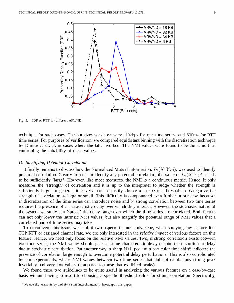
It is important to note that the time shift between two time-series being correlated could be stochasticin nature. This is true, for example, when correlating the data sending rate and the data receiving ratetime-series. In order to capture any potential correlation, one needs to account for the one-way propagationdelay in the network. If the network’s round trip time is uniformly distributed then one cannot expectto capture any correlation by considering constant time shifts between the two time series. In all ourexperiments, however, the round trip time distribution did have a dominant peak at some fixed constantvalue as shown in Fig. 3. NMI will simply capture any potential correlation between the two time seriesat that dominant time shift which is sufficient for the purposes of our study.

C. Time Series Discretization

Observe from Eqn. 3 that in order to use mutual information to quantify the correlation between twotime series, we need to estimate the marginal and joint probability distributions of both time series. Sincetime series like RTT are real-valued, they must be discretized for this purpose. Towards this end weutilized two techniques for discretization5.

The first technique we used was proposed by Dimitrova et al. [12] which seeks to ’bin’ any real-valuedtime series data into a finite number of discrete values. The algorithm assumes no knowledge about thedistribution, range or discretization thresholds of the data. It is based on the single-link clustering (SLC)algorithm and aims to minimize the information loss (measured by the entropy), which is inherent to anydiscretization. The algorithm has also been shown to maintain prior correlation between the original timeseries, which was one of our main criteria for the selection of this technique.

Although we found the technique to be quite effective, the range of time series behavior in ourexperiments is quite large and there were cases where discretization by this technique fails to captureimportant properties. This was especially significant in cases with slowly varying signals with suddenvariations. Hence, we also utilized standard binning with equidistant bin sizes as an alternate discretization

5Most of the time series we were correlating were discrete in nature thus allowing us to model them as discrete random variables.


0 1 2 3 4 50

0.05

0.1

0.15

0.2

0.25

0.3

0.35

0.4

0.45

0.5

RTT (Seconds)

Prob

abilit

y D

ensi

ty F

unct

ion

(PD

F)

ARWND = 16 KBARWND = 32 KBARWND = 64 KBARWND = 8 KB

Fig. 3. PDF of RTT for different ARWND

technique for such cases. The bin sizes we chose were: 10kbps for rate time series, and 500ms for RTTtime series. For purposes of verification, we compared equidistant binning with the discretization techniqueby Dimitrova et. al. in cases where the latter worked. The NMI values were found to be the same thusconfirming the suitability of these values.

D. Identifying Potential Correlation

It finally remains to discuss how the Normalized Mutual Information, IN(X; Y ; d), was used to identifypotential correlation. Clearly in order to identify any potential correlation, the value of IN(X, Y ; d) needsto be sufficiently ’large’. However, like most measures, the NMI is a continuous metric. Hence, it onlymeasures the ’strength’ of correlation and it is up to the interpreter to judge whether the strength issufficiently large. In general, it is very hard to justify choice of a specific threshold to categorize thestrength of correlation as large or small. This difficulty is compounded even further in our case because:a) discretization of the time series can introduce noise and b) strong correlation between two time seriesrequires the presence of a characteristic delay over which they interact. However, the stochastic nature ofthe system we study can ’spread’ the delay range over which the time series are correlated. Both factorscan not only lower the intrinsic NMI values, but also magnify the potential range of NMI values that acorrelated pair of time series may take.

To circumvent this issue, we exploit two aspects in our study. One, when studying any feature likeTCP RTT or assigned channel rate, we are only interested in the relative impact of various factors on thisfeature. Hence, we need only focus on the relative NMI values. Two, if strong correlation exists betweentwo time series, the NMI values should peak at some characteristic delay despite the distortion in delaydue to stochastic perturbation. Put another way, a sharp NMI peak at a particular time shift6 indicates thepresence of correlation large enough to overcome potential delay perturbations. This is also corroboratedby our experiments, where NMI values between two time series that did not exhibit any strong peakinvariably had very low values (compared to those that exhibited peaks).

We found these two guidelines to be quite useful in analyzing the various features on a case-by-casebasis without having to resort to choosing a specific threshold value for strong correlation. Specifically,

6We use the terms delay and time shift interchangeably throughput this paper.


when studying the impact of various factors on a given feature, as a first step the sharpness of the NMIcurves as a function of the time shifts helps narrow the potential correlations. The peak value of the NMIcurve for each factor is then used to rank the relative strength of correlation.

E. Analysis at Multiple Time Scales: Wavelets

The last aspect of evaluation that we wish to touch upon is the time scale of different events. Specifically,some RF factors like channel rate, RLP re-transmissions and channel conditions vary over a very smalltime scale7 while others like the sector load change more slowly. Similarly, TCP reacts at the time scaleof round trip times, which for wireless links, we show can be in the order of seconds.

Consequently, it is of interest to study the correlation between time series of various parameters atdifferent time scales. For example, an important case that we study is whether changes in TCP sendingrate at small time-scales are correlated to the rapid variations in the wireless channel rate.

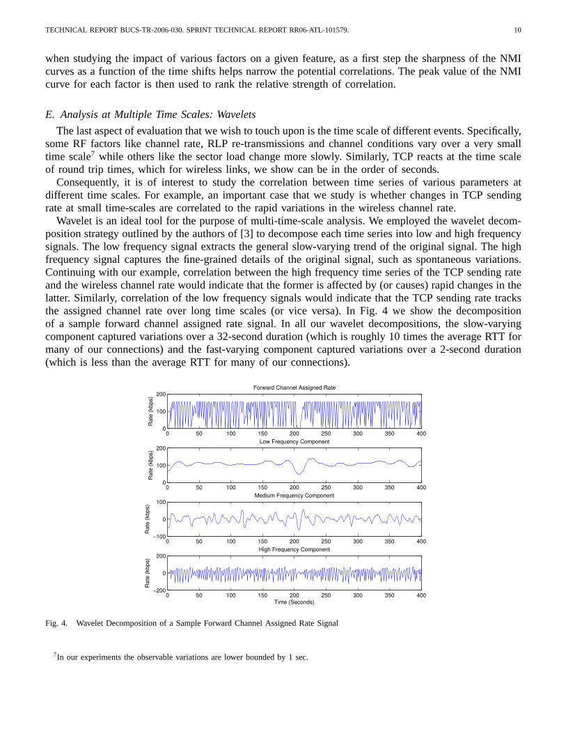
Wavelet is an ideal tool for the purpose of multi-time-scale analysis. We employed the wavelet decom-position strategy outlined by the authors of [3] to decompose each time series into low and high frequencysignals. The low frequency signal extracts the general slow-varying trend of the original signal. The highfrequency signal captures the fine-grained details of the original signal, such as spontaneous variations.Continuing with our example, correlation between the high frequency time series of the TCP sending rateand the wireless channel rate would indicate that the former is affected by (or causes) rapid changes in thelatter. Similarly, correlation of the low frequency signals would indicate that the TCP sending rate tracksthe assigned channel rate over long time scales (or vice versa). In Fig. 4 we show the decompositionof a sample forward channel assigned rate signal. In all our wavelet decompositions, the slow-varyingcomponent captured variations over a 32-second duration (which is roughly 10 times the average RTT formany of our connections) and the fast-varying component captured variations over a 2-second duration(which is less than the average RTT for many of our connections).

0 50 100 150 200 250 300 350 4000

100

200Forward Channel Assigned Rate

Rate

(kbp

s)

0 50 100 150 200 250 300 350 4000

100

200Low Frequency Component

Rate

(kbp

s)

0 50 100 150 200 250 300 350 400−100

0

100Medium Frequency Component

Rate

(kbp

s)

0 50 100 150 200 250 300 350 400−200

0

200High Frequency Component

Time (Seconds)

Rate

(kbp

s)

Fig. 4. Wavelet Decomposition of a Sample Forward Channel Assigned Rate Signal

7In our experiments the observable variations are lower bounded by 1 sec.


V. CHARACTERIZING THE WIRELESS SCHEDULER

In this section we present an empirical evaluation of the various factors that affect the behavior of thewireless scheduler. Recall from Section II-B, that the wireless scheduler’s decisions can be affected bythree factors:

• the data sending rate or buffer backlog,• the channel conditions, and• the sector loadWe quantify the impact of each of these factors in this section.

A. Impact of Data Sending Rate and Buffer Backlog

We performed numerous UDP experiments using constant bit rate (CBR), as well as on-off trafficsources where the on and off durations, as well as the peak data rate were varied. The CBR traffic sourceallows us to determine if the scheduler tracks the user’s sending rate over long time scales. An on-offtraffic source, on the other hand allows us to probe the channel with a bursty-like data source to see ifthe channel rate scheduler is able to track the data source over short time scales.

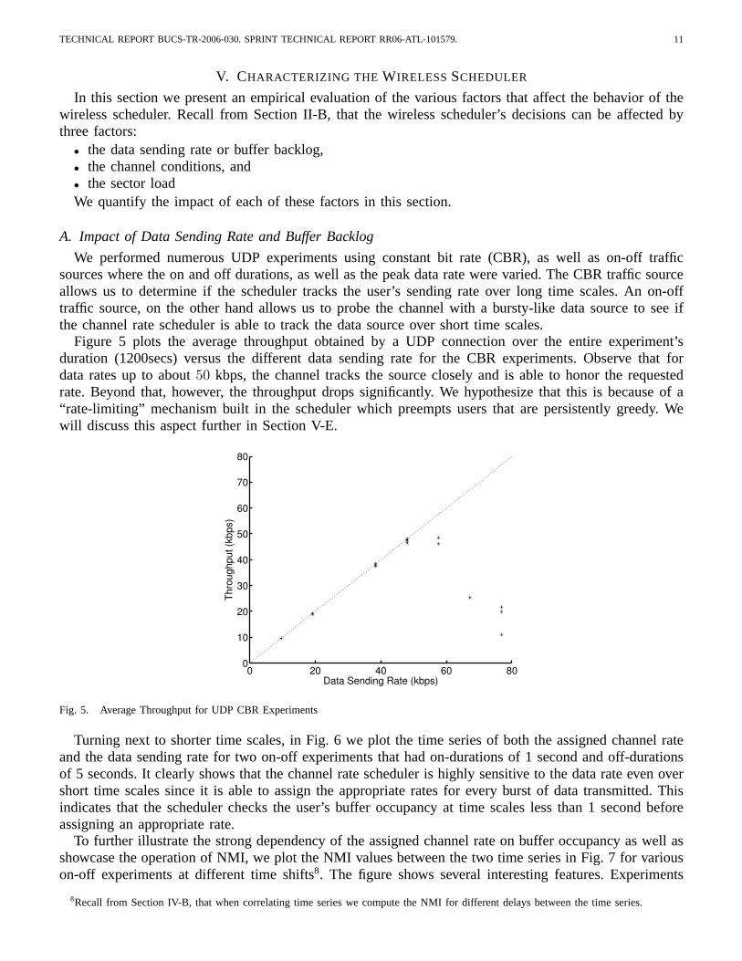
Figure 5 plots the average throughput obtained by a UDP connection over the entire experiment’sduration (1200secs) versus the different data sending rate for the CBR experiments. Observe that fordata rates up to about 50 kbps, the channel tracks the source closely and is able to honor the requestedrate. Beyond that, however, the throughput drops significantly. We hypothesize that this is because of a“rate-limiting” mechanism built in the scheduler which preempts users that are persistently greedy. Wewill discuss this aspect further in Section V-E.

0 20 40 60 800

10

20

30

40

50

60

70

80

Data Sending Rate (kbps)

Thro

ughp

ut (k

bps)

Fig. 5. Average Throughput for UDP CBR Experiments

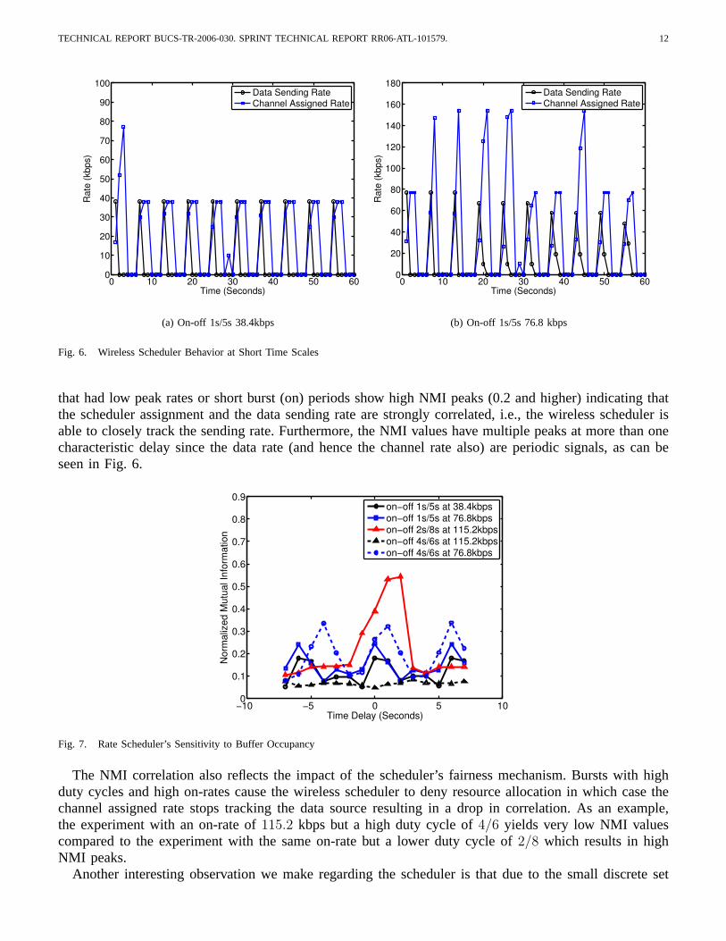
Turning next to shorter time scales, in Fig. 6 we plot the time series of both the assigned channel rateand the data sending rate for two on-off experiments that had on-durations of 1 second and off-durationsof 5 seconds. It clearly shows that the channel rate scheduler is highly sensitive to the data rate even overshort time scales since it is able to assign the appropriate rates for every burst of data transmitted. Thisindicates that the scheduler checks the user’s buffer occupancy at time scales less than 1 second beforeassigning an appropriate rate.

To further illustrate the strong dependency of the assigned channel rate on buffer occupancy as well asshowcase the operation of NMI, we plot the NMI values between the two time series in Fig. 7 for variouson-off experiments at different time shifts8. The figure shows several interesting features. Experiments

8Recall from Section IV-B, that when correlating time series we compute the NMI for different delays between the time series.


0 10 20 30 40 50 600

10

20

30

40

50

60

70

80

90

100

Time (Seconds)

Rate

(kbp

s)Data Sending RateChannel Assigned Rate

(a) On-off 1s/5s 38.4kbps

0 10 20 30 40 50 600

20

40

60

80

100

120

140

160

180

Time (Seconds)

Rate

(kbp

s)

Data Sending RateChannel Assigned Rate

(b) On-off 1s/5s 76.8 kbps

Fig. 6. Wireless Scheduler Behavior at Short Time Scales

that had low peak rates or short burst (on) periods show high NMI peaks (0.2 and higher) indicating thatthe scheduler assignment and the data sending rate are strongly correlated, i.e., the wireless scheduler isable to closely track the sending rate. Furthermore, the NMI values have multiple peaks at more than onecharacteristic delay since the data rate (and hence the channel rate also) are periodic signals, as can beseen in Fig. 6.

−10 −5 0 5 100

0.1

0.2

0.3

0.4

0.5

0.6

0.7

0.8

0.9

Time Delay (Seconds)

Nor

mal

ized

Mut

ual I

nfor

mat

ion

on−off 1s/5s at 38.4kbpson−off 1s/5s at 76.8kbpson−off 2s/8s at 115.2kbpson−off 4s/6s at 115.2kbpson−off 4s/6s at 76.8kbps

Fig. 7. Rate Scheduler’s Sensitivity to Buffer Occupancy

The NMI correlation also reflects the impact of the scheduler’s fairness mechanism. Bursts with highduty cycles and high on-rates cause the wireless scheduler to deny resource allocation in which case thechannel assigned rate stops tracking the data source resulting in a drop in correlation. As an example,the experiment with an on-rate of 115.2 kbps but a high duty cycle of 4/6 yields very low NMI valuescompared to the experiment with the same on-rate but a lower duty cycle of 2/8 which results in highNMI peaks.

Another interesting observation we make regarding the scheduler is that due to the small discrete set


of supplemental channel rates, the rate scheduler may assign a much higher rate than the one requested,as shown in Fig. 6(b), which could have implications on the stability of the system.

B. Impact of Channel Quality over Short Timescales

It is well known that channel conditions can introduce significant signal distortion. However moderntechnologies like CDMA2000 incorporate techniques like rate control (through adaptive coding, modula-tion, Walsh Code length) as well as power control that allow them to either vary the rate or increase thepower to adapt to channel conditions without sacrificing packet integrity. We wish to quantify the role ofthe former factor, i.e., adaptive changes in the channel rate assigned to the mobile in response to channelconditions, since it can directly affect higher layer protocols.

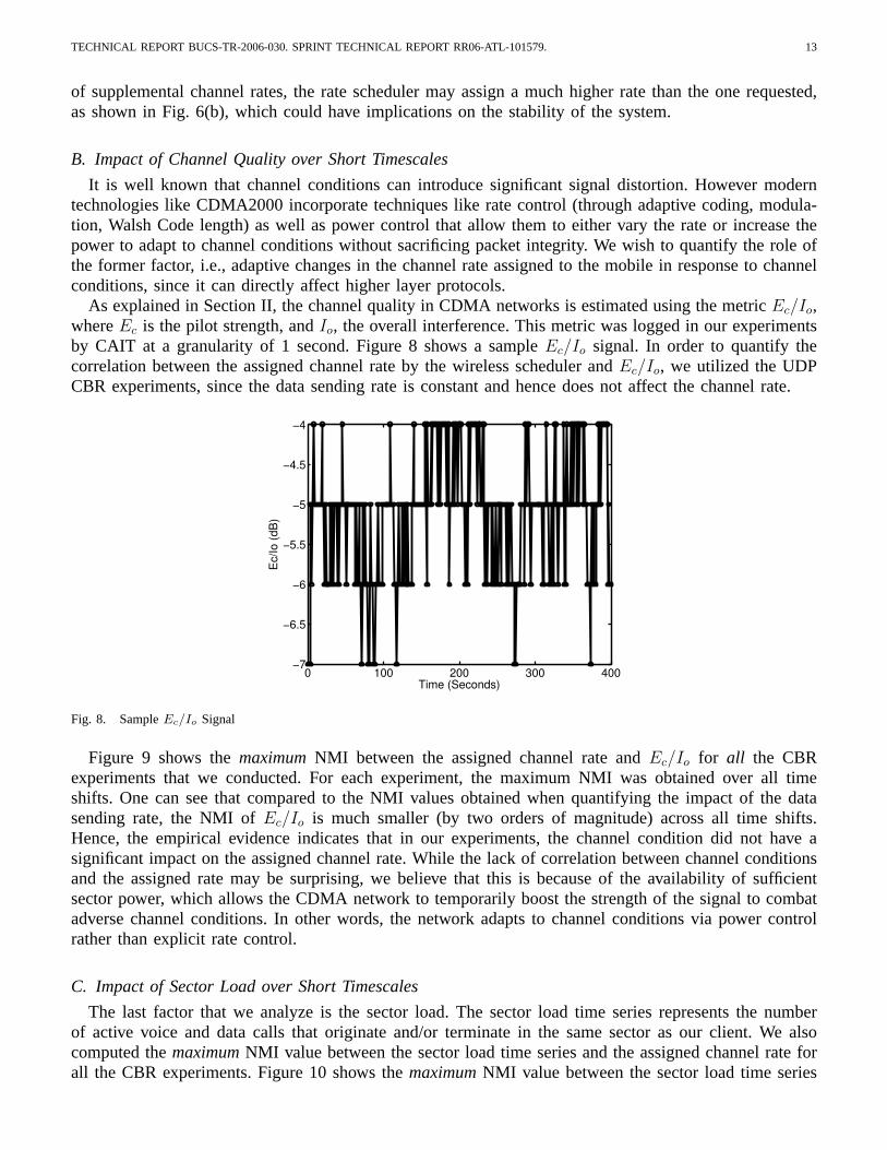
As explained in Section II, the channel quality in CDMA networks is estimated using the metric Ec/Io,where Ec is the pilot strength, and Io, the overall interference. This metric was logged in our experimentsby CAIT at a granularity of 1 second. Figure 8 shows a sample Ec/Io signal. In order to quantify thecorrelation between the assigned channel rate by the wireless scheduler and Ec/Io, we utilized the UDPCBR experiments, since the data sending rate is constant and hence does not affect the channel rate.

0 100 200 300 400−7

−6.5

−6

−5.5

−5

−4.5

−4

Time (Seconds)

Ec/Io

(dB)

Fig. 8. Sample Ec/Io Signal

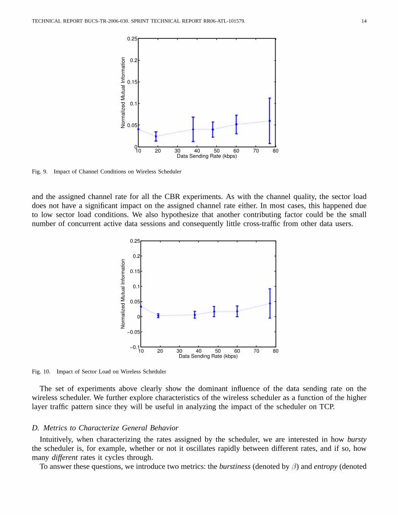
Figure 9 shows the maximum NMI between the assigned channel rate and Ec/Io for all the CBRexperiments that we conducted. For each experiment, the maximum NMI was obtained over all timeshifts. One can see that compared to the NMI values obtained when quantifying the impact of the datasending rate, the NMI of Ec/Io is much smaller (by two orders of magnitude) across all time shifts.Hence, the empirical evidence indicates that in our experiments, the channel condition did not have asignificant impact on the assigned channel rate. While the lack of correlation between channel conditionsand the assigned rate may be surprising, we believe that this is because of the availability of sufficientsector power, which allows the CDMA network to temporarily boost the strength of the signal to combatadverse channel conditions. In other words, the network adapts to channel conditions via power controlrather than explicit rate control.

C. Impact of Sector Load over Short Timescales

The last factor that we analyze is the sector load. The sector load time series represents the numberof active voice and data calls that originate and/or terminate in the same sector as our client. We alsocomputed the maximum NMI value between the sector load time series and the assigned channel rate forall the CBR experiments. Figure 10 shows the maximum NMI value between the sector load time series


10 20 30 40 50 60 70 800

0.05

0.1

0.15

0.2

0.25


Norm

alize

d M

utua

l Inf

orm

atio

n

Fig. 9. Impact of Channel Conditions on Wireless Scheduler

and the assigned channel rate for all the CBR experiments. As with the channel quality, the sector loaddoes not have a significant impact on the assigned channel rate either. In most cases, this happened dueto low sector load conditions. We also hypothesize that another contributing factor could be the smallnumber of concurrent active data sessions and consequently little cross-traffic from other data users.

10 20 30 40 50 60 70 80−0.1

−0.05

0

0.05

0.1

0.15

0.2

0.25


Norm

alize

d M

utua

l Inf

orm

atio

n

Fig. 10. Impact of Sector Load on Wireless Scheduler

The set of experiments above clearly show the dominant influence of the data sending rate on thewireless scheduler. We further explore characteristics of the wireless scheduler as a function of the higherlayer traffic pattern since they will be useful in analyzing the impact of the scheduler on TCP.

D. Metrics to Characterize General Behavior

Intuitively, when characterizing the rates assigned by the scheduler, we are interested in how burstythe scheduler is, for example, whether or not it oscillates rapidly between different rates, and if so, howmany different rates it cycles through.

To answer these questions, we introduce two metrics: the burstiness (denoted by β) and entropy (denoted


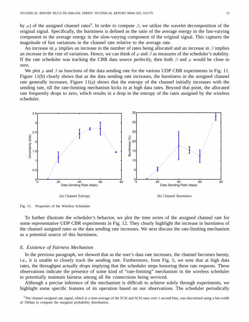
by µ) of the assigned channel rates9. In order to compute β, we utilize the wavelet decomposition of theoriginal signal. Specifically, the burstiness is defined as the ratio of the average energy in the fast-varyingcomponent to the average energy in the slow-varying component of the original signal. This captures themagnitude of fast variations in the channel rate relative to the average rate.

An increase in µ implies an increase in the number of rates being allocated and an increase in β impliesan increase in the rate of variations. Hence, we can think of µ and β as measures of the scheduler’s stability.If the rate scheduler was tracking the CBR data source perfectly, then both β and µ would be close tozero.

We plot µ and β as functions of the data sending rate for the various UDP CBR experiments in Fig. 11.Figure 11(b) clearly shows that as the data sending rate increases, the burstiness in the assigned channelrate generally increases. Figure 11(a) shows that the entropy of the channel initially increases with thesending rate, till the rate-limiting mechanism kicks in at high data rates. Beyond that point, the allocatedrate frequently drops to zero, which results in a drop in the entropy of the rates assigned by the wirelessscheduler.

0 20 40 60 800

0.5

1

1.5

2

2.5

3

3.5


Unce

rtain

ty (b

its)

(a) Channel Entropy

0 20 40 60 800

5

10

15

20

25

30

35


Burs

tines

s (%

)

(b) Channel Burstiness

Fig. 11. Properties of the Wireless Scheduler

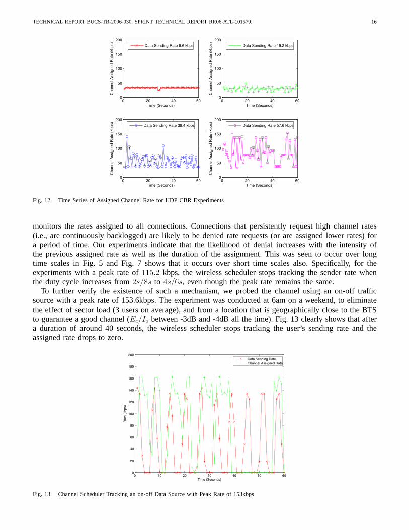
To further illustrate the scheduler’s behavior, we plot the time series of the assigned channel rate forsome representative UDP CBR experiments in Fig. 12. They clearly highlight the increase in burstiness ofthe channel assigned rates as the data sending rate increases. We next discuss the rate-limiting mechanismas a potential source of this burstiness.

E. Existence of Fairness Mechanism

In the previous paragraph, we showed that as the user’s data rate increases, the channel becomes bursty,i.e., it is unable to closely track the sending rate. Furthermore, from Fig. 5, we note that at high datarates, the throughput actually drops implying that the scheduler stops honoring these rate requests. Theseobservations indicate the presence of some kind of “rate-limiting” mechanism in the wireless schedulerto potentially maintain fairness among all the connections being serviced.

Although a precise inference of the mechanism is difficult to achieve solely through experiments, wehighlight some specific features of its operation based on our observations. The scheduler periodically

9The channel assigned rate signal, which is a time-average of the FCH and SCH rates over 1 second bins, was discretized using a bin-widthof 10kbps to compute the marginal probability distribution.


0 20 40 600

50

100

150

200

Time (Seconds)

Cha

nnel

Ass

igne

d R

ate

(kbp

s) Data Sending Rate 9.6 kbps

0 20 40 600

50

100

150

200

Time (Seconds)

Cha

nnel

Ass

igne

d R

ate

(kbp


0 20 40 600

50

100

150

200

Time (Seconds)

Cha

nnel

Ass

igne

d R

ate

(kbp


0 20 40 600

50

100

150

200

Time (Seconds)

Cha

nnel

Ass

igne

d R

ate

(kbp


Fig. 12. Time Series of Assigned Channel Rate for UDP CBR Experiments

monitors the rates assigned to all connections. Connections that persistently request high channel rates(i.e., are continuously backlogged) are likely to be denied rate requests (or are assigned lower rates) fora period of time. Our experiments indicate that the likelihood of denial increases with the intensity ofthe previous assigned rate as well as the duration of the assignment. This was seen to occur over longtime scales in Fig. 5 and Fig. 7 shows that it occurs over short time scales also. Specifically, for theexperiments with a peak rate of 115.2 kbps, the wireless scheduler stops tracking the sender rate whenthe duty cycle increases from 2s/8s to 4s/6s, even though the peak rate remains the same.

To further verify the existence of such a mechanism, we probed the channel using an on-off trafficsource with a peak rate of 153.6kbps. The experiment was conducted at 6am on a weekend, to eliminatethe effect of sector load (3 users on average), and from a location that is geographically close to the BTSto guarantee a good channel (Ec/Io between -3dB and -4dB all the time). Fig. 13 clearly shows that aftera duration of around 40 seconds, the wireless scheduler stops tracking the user’s sending rate and theassigned rate drops to zero.

0 10 20 30 40 50 600

20

40

60

80

100

120

140

160

180

200

Time (Seconds)

Rat

e (k

bps)


Fig. 13. Channel Scheduler Tracking an on-off Data Source with Peak Rate of 153kbps


VI. CHARACTERIZING THE RADIO LINK PROTOCOL

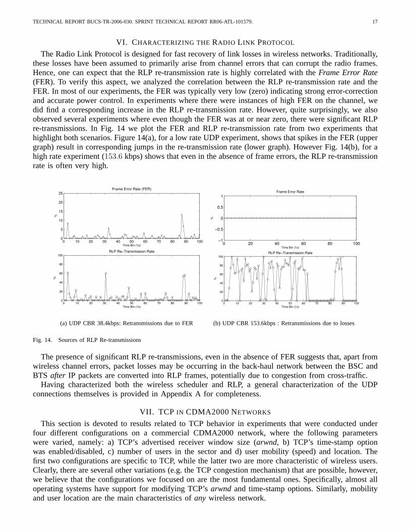
The Radio Link Protocol is designed for fast recovery of link losses in wireless networks. Traditionally,these losses have been assumed to primarily arise from channel errors that can corrupt the radio frames.Hence, one can expect that the RLP re-transmission rate is highly correlated with the Frame Error Rate(FER). To verify this aspect, we analyzed the correlation between the RLP re-transmission rate and theFER. In most of our experiments, the FER was typically very low (zero) indicating strong error-correctionand accurate power control. In experiments where there were instances of high FER on the channel, wedid find a corresponding increase in the RLP re-transmission rate. However, quite surprisingly, we alsoobserved several experiments where even though the FER was at or near zero, there were significant RLPre-transmissions. In Fig. 14 we plot the FER and RLP re-transmission rate from two experiments thathighlight both scenarios. Figure 14(a), for a low rate UDP experiment, shows that spikes in the FER (uppergraph) result in corresponding jumps in the re-transmission rate (lower graph). However Fig. 14(b), for ahigh rate experiment (153.6 kbps) shows that even in the absence of frame errors, the RLP re-transmissionrate is often very high.

0 10 20 30 40 50 60 70 80 90 1000

5

10

15

20

25

Time Bin (1s)

%

Frame Error Rate (FER)

0 10 20 30 40 50 60 70 80 90 1000

20

40

60

80

100

Time Bin (1s)

%

RLP Re−Transmission Rate

(a) UDP CBR 38.4kbps: Retransmissions due to FER

0 20 40 60 80 100−1

−0.5

0

0.5

1

Time Bin (1s)

%

Frame Error Rate

0 10 20 30 40 50 60 70 80 90 1000

20

40

60

80

100

Time Bin (1s)

%

RLP Re−Transmission Rate

(b) UDP CBR 153.6kbps : Retransmissions due to losses

Fig. 14. Sources of RLP Re-transmissions

The presence of significant RLP re-transmissions, even in the absence of FER suggests that, apart fromwireless channel errors, packet losses may be occurring in the back-haul network between the BSC andBTS after IP packets are converted into RLP frames, potentially due to congestion from cross-traffic.

Having characterized both the wireless scheduler and RLP, a general characterization of the UDPconnections themselves is provided in Appendix A for completeness.

VII. TCP IN CDMA2000 NETWORKS

This section is devoted to results related to TCP behavior in experiments that were conducted underfour different configurations on a commercial CDMA2000 network, where the following parameterswere varied, namely: a) TCP’s advertised receiver window size (arwnd, b) TCP’s time-stamp optionwas enabled/disabled, c) number of users in the sector and d) user mobility (speed) and location. Thefirst two configurations are specific to TCP, while the latter two are more characteristic of wireless users.Clearly, there are several other variations (e.g. the TCP congestion mechanism) that are possible, however,we believe that the configurations we focused on are the most fundamental ones. Specifically, almost alloperating systems have support for modifying TCP’s arwnd and time-stamp options. Similarly, mobilityand user location are the main characteristics of any wireless network.


Before discussing the experimental results, it is worthwhile making a general observation regarding ourresults. In almost all configurations, we found that the achieved throughput varied over a large range ofvalues (more than 10%), even across consecutive runs of the same experiment, depending on location andtime. Our measurements indicate that these variations in capacity were not caused by the channel qualityor sector load. Instead, we believe they may have to do with dynamic cell-dimensioning for neighboringcells by the network operator which is the focus of our future work.

A. TCP Window Size and Time-stamp Option

The first two configurations we study involve TCP’s behavior as a function of the advertised receiverwindow, both when the time-stamp option [22] was disabled/enabled. The window size was varied from8 KB to 128 KB.

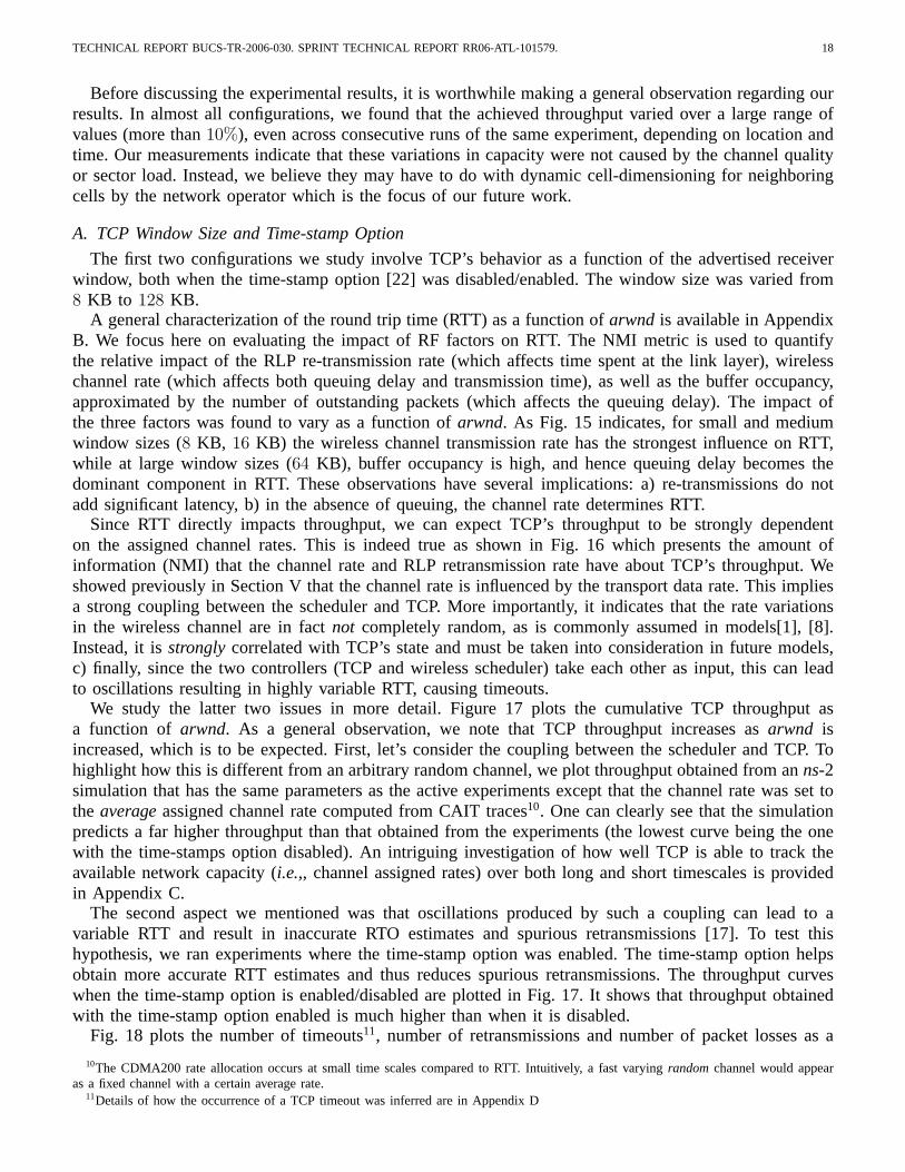
A general characterization of the round trip time (RTT) as a function of arwnd is available in AppendixB. We focus here on evaluating the impact of RF factors on RTT. The NMI metric is used to quantifythe relative impact of the RLP re-transmission rate (which affects time spent at the link layer), wirelesschannel rate (which affects both queuing delay and transmission time), as well as the buffer occupancy,approximated by the number of outstanding packets (which affects the queuing delay). The impact ofthe three factors was found to vary as a function of arwnd. As Fig. 15 indicates, for small and mediumwindow sizes (8 KB, 16 KB) the wireless channel transmission rate has the strongest influence on RTT,while at large window sizes (64 KB), buffer occupancy is high, and hence queuing delay becomes thedominant component in RTT. These observations have several implications: a) re-transmissions do notadd significant latency, b) in the absence of queuing, the channel rate determines RTT.

Since RTT directly impacts throughput, we can expect TCP’s throughput to be strongly dependenton the assigned channel rates. This is indeed true as shown in Fig. 16 which presents the amount ofinformation (NMI) that the channel rate and RLP retransmission rate have about TCP’s throughput. Weshowed previously in Section V that the channel rate is influenced by the transport data rate. This impliesa strong coupling between the scheduler and TCP. More importantly, it indicates that the rate variationsin the wireless channel are in fact not completely random, as is commonly assumed in models[1], [8].Instead, it is strongly correlated with TCP’s state and must be taken into consideration in future models,c) finally, since the two controllers (TCP and wireless scheduler) take each other as input, this can leadto oscillations resulting in highly variable RTT, causing timeouts.

We study the latter two issues in more detail. Figure 17 plots the cumulative TCP throughput asa function of arwnd. As a general observation, we note that TCP throughput increases as arwnd isincreased, which is to be expected. First, let’s consider the coupling between the scheduler and TCP. Tohighlight how this is different from an arbitrary random channel, we plot throughput obtained from an ns-2simulation that has the same parameters as the active experiments except that the channel rate was set tothe average assigned channel rate computed from CAIT traces10. One can clearly see that the simulationpredicts a far higher throughput than that obtained from the experiments (the lowest curve being the onewith the time-stamps option disabled). An intriguing investigation of how well TCP is able to track theavailable network capacity (i.e.,, channel assigned rates) over both long and short timescales is providedin Appendix C.

The second aspect we mentioned was that oscillations produced by such a coupling can lead to avariable RTT and result in inaccurate RTO estimates and spurious retransmissions [17]. To test thishypothesis, we ran experiments where the time-stamp option was enabled. The time-stamp option helpsobtain more accurate RTT estimates and thus reduces spurious retransmissions. The throughput curveswhen the time-stamp option is enabled/disabled are plotted in Fig. 17. It shows that throughput obtainedwith the time-stamp option enabled is much higher than when it is disabled.

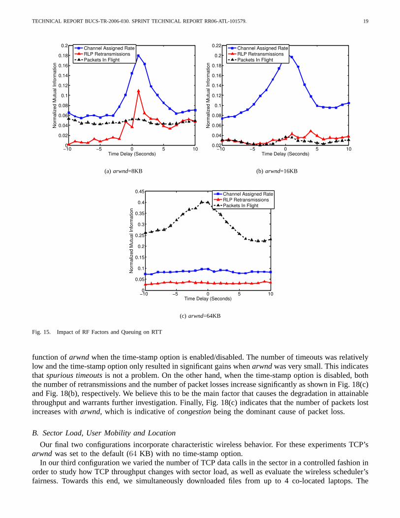
Fig. 18 plots the number of timeouts11, number of retransmissions and number of packet losses as a

10The CDMA200 rate allocation occurs at small time scales compared to RTT. Intuitively, a fast varying random channel would appearas a fixed channel with a certain average rate.

11Details of how the occurrence of a TCP timeout was inferred are in Appendix D


−10 −5 0 5 100

0.02

0.04

0.06

0.08

0.1

0.12

0.14

0.16

0.18

0.2


Nor

mal

ized

Mut

ual I

nfor

mat

ion

Channel Assigned RateRLP RetransmissionsPackets In Flight

(a) arwnd=8KB

−10 −5 0 5 100.02

0.04

0.06

0.08

0.1

0.12

0.14

0.16

0.18

0.2

0.22


Nor

mal

ized

Mut

ual I

nfor

mat

ion


(b) arwnd=16KB

−10 −5 0 5 100

0.05

0.1

0.15

0.2

0.25

0.3

0.35

0.4

0.45


Nor

mal

ized

Mut

ual I

nfor

mat

ion


(c) arwnd=64KB

Fig. 15. Impact of RF Factors and Queuing on RTT

function of arwnd when the time-stamp option is enabled/disabled. The number of timeouts was relativelylow and the time-stamp option only resulted in significant gains when arwnd was very small. This indicatesthat spurious timeouts is not a problem. On the other hand, when the time-stamp option is disabled, boththe number of retransmissions and the number of packet losses increase significantly as shown in Fig. 18(c)and Fig. 18(b), respectively. We believe this to be the main factor that causes the degradation in attainablethroughput and warrants further investigation. Finally, Fig. 18(c) indicates that the number of packets lostincreases with arwnd, which is indicative of congestion being the dominant cause of packet loss.

B. Sector Load, User Mobility and Location

Our final two configurations incorporate characteristic wireless behavior. For these experiments TCP’sarwnd was set to the default (64 KB) with no time-stamp option.

In our third configuration we varied the number of TCP data calls in the sector in a controlled fashion inorder to study how TCP throughput changes with sector load, as well as evaluate the wireless scheduler’sfairness. Towards this end, we simultaneously downloaded files from up to 4 co-located laptops. The


−15 −10 −5 0 5 10 150

0.02

0.04

0.06

0.08

0.1

0.12

0.14

0.16


Nor

mal

ized

Mut

ual I

nfor

mat

ion

Channel Assigned RateRLP Retransmissions

(a) arwnd=8KB

−15 −10 −5 0 5 10 150

0.05

0.1

0.15

0.2

0.25

0.3

0.35


Nor

mal

ized

Mut

ual I

nfor

mat

ion

Channel Assigned RateRLP Retransmissions

(b) arwnd=64KB

Fig. 16. Factors Affecting Instantaneous TCP Throughput

0 20 40 60 80 100 120 14020

40

60

80

100

120

140

160

Advertized Receiver Window (KB)

TCP

Thro

ughp

ut (k

bps)

SimulationsTCP with SACK and Timestamps EnabledTCP with SACK Enabled

Fig. 17. TCP throughput as a function of arwnd

experiments were conducted at off-peak hours to ensure that the only users in the sector were theexperiment laptops12. In Fig. 19 we plot the cumulative TCP throughput (on the left), as well as Jain’sFairness Index[14] (on the right) as a function of the number of active users. Jain’s Fairness Index liesbetween 0 and 1. A value of 1 indicates a throughput-fair allocation. For any given set of throughputs(y1, y2,...,yn), it is calculated as:

g(y1, y2, ...yn) =(∑n

i=1 yi)2

n.∑n

i=1 y2i

(7)

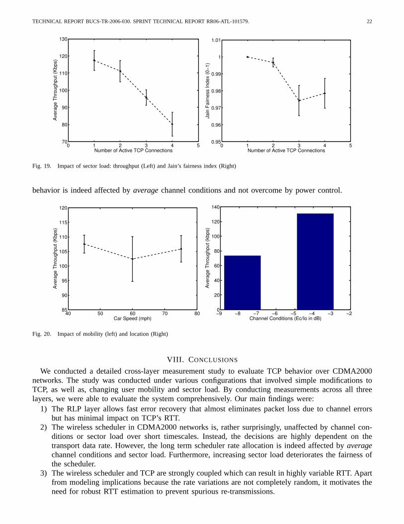
Not surprisingly, the average throughput achieved per user decreases with the number of connections.However, we note that the fairness of the scheduler degrades with number of connections, as reflected bya lower index value. Indeed, manual inspection of our experiments indicate that the throughput achievedby concurrent connections can be highly disparate with typically one user dominating.

The final configuration involved evaluating the impact of user mobility and location on performance.For our mobility experiments, we ran TCP downloads while traveling on a major highway (US-101)

12This was verified independently by logging the PCMD data.


0 20 40 60 80 100 120 140−2

0

2

4

6

8

10

12Nu

mbe

r of T

imeo

uts


Timestamp Option EnabledTimestamp Option Disabled

(a) Timeouts

0 20 40 60 80 100 120 1400

20

40

60

80

100

120

Num

ber o

f Ret

rans

miss

ions



(b) Retransmissions

0 20 40 60 80 100 120 1400

10

20

30

40

50

60

70

80

90

100

Num

ber o

f Pac

kets

Los

t



(c) Packet Loss

Fig. 18. TCP timeouts, retransmissions and packet loss

during off-peak hours. Figure 20 (Left) shows the achieved TCP throughput for three different averagespeeds of 45, 60 and 75 mph, respectively. Surprisingly, user speed had little impact on TCP throughputindicating that the cellular network is well engineered for fast hand-offs. We note that mobility is a majorconcern in 802.11 networks which are not a priori designed to handle fast transitions.

The last set of experiments were conducted to investigate the impact of average (long-term) channelconditions. In Section V we showed that the short-term scheduler behavior was unaffected by instantaneousvariations in channel conditions. However, it is unclear whether this observation carries over to channelconditions over longer timescales. To investigate this, we performed two sets of experiments, where thelaptop was placed in locations with either consistently good or bad channels13. The average throughputfor each location is plotted in Fig. 20 (Right)14. One can clearly see that the throughput at a locationwith better channel conditions (higher Ec/I0) is much higher. This indicates that the long-term scheduler

13This was verified by logging the Ec/Io with CAIT.14The RTT and general path characteristics for both locations were very similar.


0 1 2 3 4 570

80

90

100

110

120

130

Number of Active TCP Connections

Aver

age

Thro

ughp

ut (K

bps)

0 1 2 3 4 50.95

0.96

0.97

0.98

0.99

1

1.01

Number of Active TCP Connections

Jain

Fai

rnes

s In

dex

(0−1

)

Fig. 19. Impact of sector load: throughput (Left) and Jain’s fairness index (Right)

behavior is indeed affected by average channel conditions and not overcome by power control.

40 50 60 70 8085

90

95

100

105

110

115

120

Car Speed (mph)

Aver

age

Thro

ughp

ut (K

bps)

−9 −8 −7 −6 −5 −4 −3 −20

20

40

60

80

100

120

140

Channel Conditions (Ec/Io in dB)

Aver

age

Thro

ughp

ut (k

bps)

Fig. 20. Impact of mobility (left) and location (Right)

VIII. CONCLUSIONS

We conducted a detailed cross-layer measurement study to evaluate TCP behavior over CDMA2000networks. The study was conducted under various configurations that involved simple modifications toTCP, as well as, changing user mobility and sector load. By conducting measurements across all threelayers, we were able to evaluate the system comprehensively. Our main findings were:

1) The RLP layer allows fast error recovery that almost eliminates packet loss due to channel errorsbut has minimal impact on TCP’s RTT.

2) The wireless scheduler in CDMA2000 networks is, rather surprisingly, unaffected by channel con-ditions or sector load over short timescales. Instead, the decisions are highly dependent on thetransport data rate. However, the long term scheduler rate allocation is indeed affected by averagechannel conditions and sector load. Furthermore, increasing sector load deteriorates the fairness ofthe scheduler.

3) The wireless scheduler and TCP are strongly coupled which can result in highly variable RTT. Apartfrom modeling implications because the rate variations are not completely random, it motivates theneed for robust RTT estimation to prevent spurious re-transmissions.


4) Mobility in the CDMA2000 network had no major impact on TCP throughput.

APPENDIX

Appendix A: UDP Connections: RTT, Packet Loss, and ReorderingBefore analyzing the interaction between the wireless channel and TCP, here we give some preliminary

insight into higher layer metrics important for TCP performance, such as RTT, packet loss, and packetreordering that were experienced by the UDP connections. This will aid in our discussions regarding TCPin Section VII.

The client in our UDP application responded to received packets with acknowledgments (the server’stransmission rate is not influenced by this). The data packets and acknowledgments had sequence numbersthat allowed us to compute the RTT, identify the packets that were lost and infer any potential reorderingof packets.

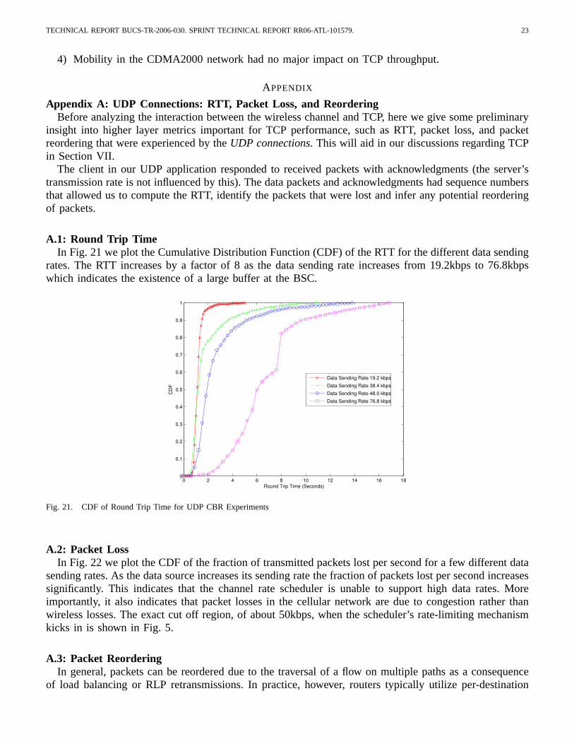
A.1: Round Trip TimeIn Fig. 21 we plot the Cumulative Distribution Function (CDF) of the RTT for the different data sending

rates. The RTT increases by a factor of 8 as the data sending rate increases from 19.2kbps to 76.8kbpswhich indicates the existence of a large buffer at the BSC.

0 2 4 6 8 10 12 14 16 180

0.1

0.2

0.3

0.4

0.5

0.6

0.7

0.8

0.9

1

Round Trip Time (Seconds)

CDF

Data Sending Rate 19.2 kbpsData Sending Rate 38.4 kbpsData Sending Rate 48.0 kbpsData Sending Rate 76.8 kbps

Fig. 21. CDF of Round Trip Time for UDP CBR Experiments

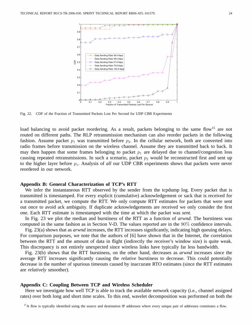
A.2: Packet LossIn Fig. 22 we plot the CDF of the fraction of transmitted packets lost per second for a few different data

sending rates. As the data source increases its sending rate the fraction of packets lost per second increasessignificantly. This indicates that the channel rate scheduler is unable to support high data rates. Moreimportantly, it also indicates that packet losses in the cellular network are due to congestion rather thanwireless losses. The exact cut off region, of about 50kbps, when the scheduler’s rate-limiting mechanismkicks in is shown in Fig. 5.

A.3: Packet ReorderingIn general, packets can be reordered due to the traversal of a flow on multiple paths as a consequence

of load balancing or RLP retransmissions. In practice, however, routers typically utilize per-destination


0 0.1 0.2 0.3 0.4 0.5 0.6 0.7 0.8 0.9 10

0.1

0.2

0.3

0.4

0.5

0.6

0.7

0.8

0.9

1

Fraction of Transmitted Packets Lost Per Second

CD

F

Data Sending Rate 38.4 kbps





Fig. 22. CDF of the Fraction of Transmitted Packets Lost Per Second for UDP CBR Experiments

load balancing to avoid packet reordering. As a result, packets belonging to the same flow15 are notrouted on different paths. The RLP retransmission mechanism can also reorder packets in the followingfashion. Assume packet p1 was transmitted before p2. In the cellular network, both are converted intoradio frames before transmission on the wireless channel. Assume they are transmitted back to back. Itmay then happen that some frames belonging to packet p1 are delayed due to channel/congestion losscausing repeated retransmissions. In such a scenario, packet p2 would be reconstructed first and sent upto the higher layer before p1. Analysis of all our UDP CBR experiments shows that packets were neverreordered in our network.

Appendix B: General Characterization of TCP’s RTTWe infer the instantaneous RTT observed by the sender from the tcpdump log. Every packet that is

transmitted is timestamped. For every explicit (cumulative) acknowledgement or sack that is received fora transmitted packet, we compute the RTT. We only compute RTT estimates for packets that were sentout once to avoid ack ambiguity. If duplicate acknowledgements are received we only consider the firstone. Each RTT estimate is timestamped with the time at which the packet was sent.

In Fig. 23 we plot the median and burstiness of the RTT as a function of arwnd. The burstiness wascomputed in the same fashion as in Section V-D. The values reported are in the 90% confidence intervals.

Fig. 23(a) shows that as arwnd increases, the RTT increases significantly, indicating high queuing delays.For comparison purposes, we note that the authors of [6] have shown that in the Internet, the correlationbetween the RTT and the amount of data in flight (indirectly the receiver’s window size) is quite weak.This discrepancy is not entirely unexpected since wireless links have typically far less bandwidth.

Fig. 23(b) shows that the RTT burstiness, on the other hand, decreases as arwnd increases since theaverage RTT increases significantly causing the relative burstiness to decrease. This could potentiallydecrease in the number of spurious timeouts caused by inaccurate RTO estimates (since the RTT estimatesare relatively smoother).

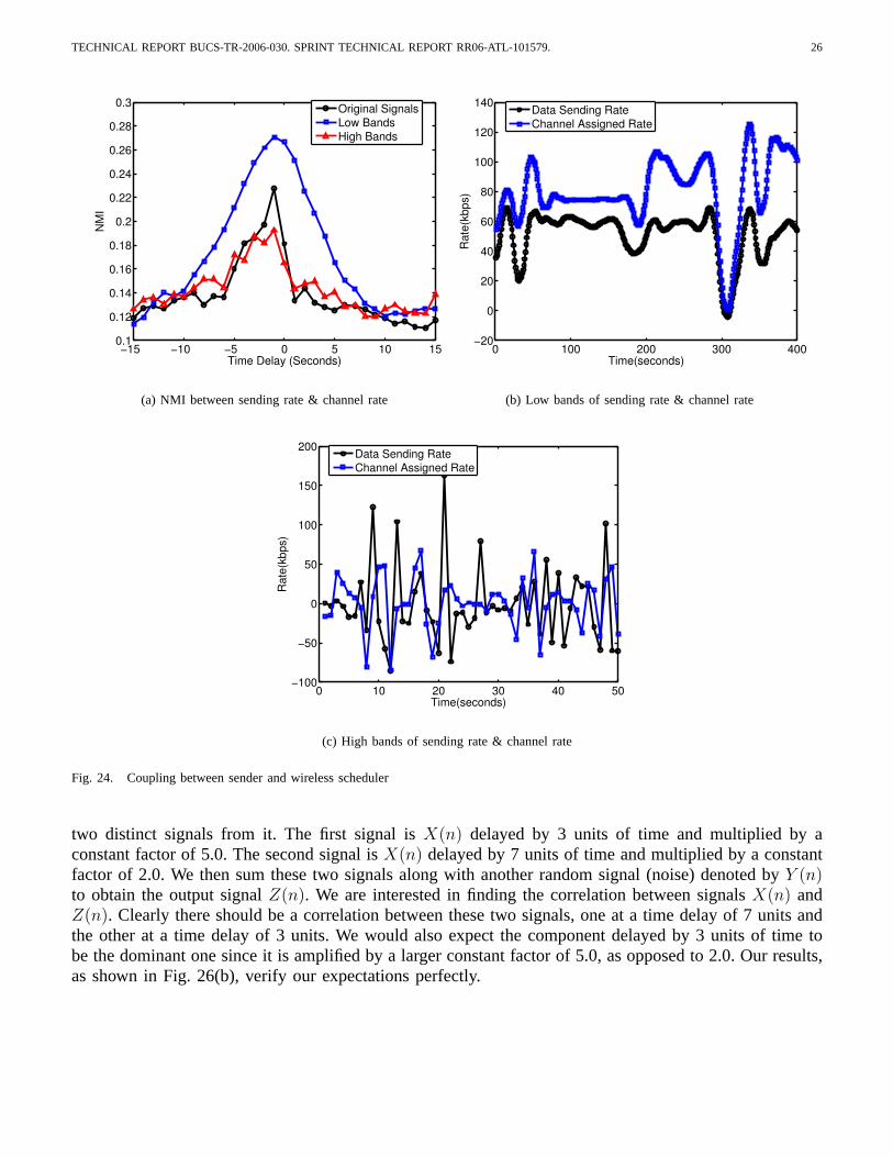
Appendix C: Coupling Between TCP and Wireless SchedulerHere we investigate how well TCP is able to track the available network capacity (i.e., channel assigned

rates) over both long and short time scales. To this end, wavelet decomposition was performed on both the

15A flow is typically identified using the source and destination IP addresses where every unique pair of addresses constitutes a flow.


0 10 20 30 40 50 60 701.5

2

2.5

3

3.5

4


Med

ian

RTT

(Sec

onds

)Median Round Trip Time Versus Advertised Receiver Window

(a) Median RTT

0 10 20 30 40 50 60 700

0.2

0.4

0.6

0.8

1

1.2

1.4

1.6

1.8


RTT

Burs

tines

s (%

)

RTT Burstiness Versus Advertised Receiver Window

(b) RTT burstiness

Fig. 23. RTT behavior as a function of ARWND

data sending rate and channel assigned rate time series to obtain their constituent low and high frequencysignals.

In Fig. 24, we plot the NMI between the high and low frequency signals and for completeness, theoriginal signals as well. We also plot the low and high frequency signals in Figures 24(b) and 24(c)respectively. From the high NMI values it is clear, that the sender and the wireless scheduler are tightlycoupled over both long and short timescales, with a stronger inter-dependence over long timescales. Inother words, the rates assigned by the wireless scheduler are highly dependent on the data sending rateover long timescales, and vice versa.

Appendix D: Inferring TCP TimeoutsIn general, a timeout can be detected when a packet is retransmitted and cwnd drops to 1 segment16

and TCP starts operating in the slow-start phase. We inferred timeouts from the tcpdump log collectedat the server. In any TCP version (including the Sack Enabled Linux TCP [21] we are using), a packetis retransmitted either due to 1) the reception of 3 duplicate acks, 2) the reception of an ack includingsacked blocks, or 3) timer expiration. In the first two cases the retransmission occurs shortly after receivingan ack from the client. In the third case, on the other hand, the retransmission does not have to occurafter receiving an ack from the client. Our timeout inference algorithm is a threshold-based separationof cases 1 and 2 from 3. In Fig. 25 we show a histogram of the time delay between the occurrence ofa retransmission and the reception of the last ack from the client across all our TCP experiments. Thetwo bars represent the total number of retransmissions that occurred within less than 10ms and more than100ms of the last ack received. There is a noticeable gap between the two bars (between 10ms and 100ms)where no retransmissions occurred. We therefore used a threshold of 100ms to distinguish between fastretransmissions and timeout-triggered retransmissions.

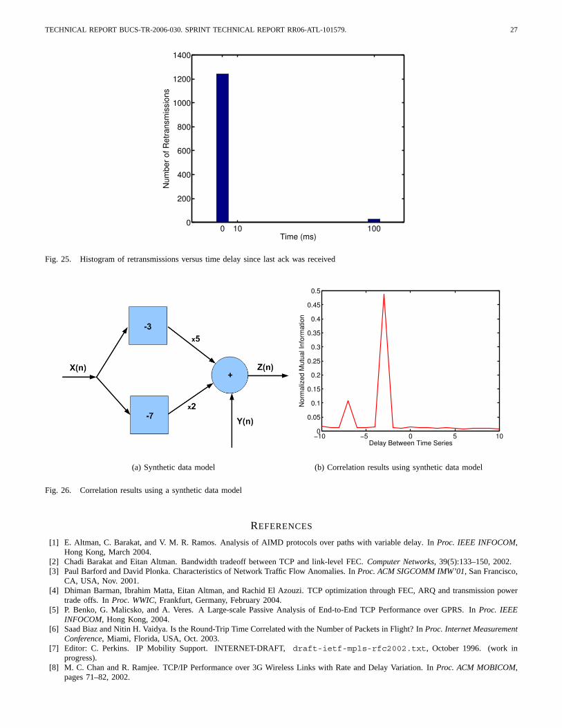
Appendix E: Synthetic Data Model and Sample Correlation ExampleIn order to test our correlation technique we used a simple synthetic data model, shown in Fig. 26(a)

that is identical to the one in [13]. In this model we take a completely random signal X(n) and create

16Some TCP implementations set the cwnd to 2 segments after a timeout is detected.


−15 −10 −5 0 5 10 150.1

0.12

0.14

0.16

0.18

0.2

0.22

0.24

0.26

0.28

0.3


NM

IOriginal SignalsLow BandsHigh Bands

(a) NMI between sending rate & channel rate

0 100 200 300 400−20

0

20

40

60

80

100

120

140

Rat

e(kb

ps)

Time(seconds)


(b) Low bands of sending rate & channel rate

0 10 20 30 40 50−100

−50

0

50

100

150

200

Rate

(kbp

s)

Time(seconds)


(c) High bands of sending rate & channel rate

Fig. 24. Coupling between sender and wireless scheduler

two distinct signals from it. The first signal is X(n) delayed by 3 units of time and multiplied by aconstant factor of 5.0. The second signal is X(n) delayed by 7 units of time and multiplied by a constantfactor of 2.0. We then sum these two signals along with another random signal (noise) denoted by Y (n)to obtain the output signal Z(n). We are interested in finding the correlation between signals X(n) andZ(n). Clearly there should be a correlation between these two signals, one at a time delay of 7 units andthe other at a time delay of 3 units. We would also expect the component delayed by 3 units of time tobe the dominant one since it is amplified by a larger constant factor of 5.0, as opposed to 2.0. Our results,as shown in Fig. 26(b), verify our expectations perfectly.


0 10 1000

200

400

600

800

1000

1200

1400

Time (ms)

Num

ber o

f Ret

rans

mis

sion

s

Fig. 25. Histogram of retransmissions versus time delay since last ack was received

(a) Synthetic data model

−10 −5 0 5 100

0.05

0.1

0.15

0.2

0.25

0.3

0.35

0.4

0.45

0.5

Delay Between Time Series

Nor

mal

ized

Mut

ual I

nfor

mat

ion

(b) Correlation results using synthetic data model

Fig. 26. Correlation results using a synthetic data model

REFERENCES

[1] E. Altman, C. Barakat, and V. M. R. Ramos. Analysis of AIMD protocols over paths with variable delay. In Proc. IEEE INFOCOM,Hong Kong, March 2004.

[2] Chadi Barakat and Eitan Altman. Bandwidth tradeoff between TCP and link-level FEC. Computer Networks, 39(5):133–150, 2002.[3] Paul Barford and David Plonka. Characteristics of Network Traffic Flow Anomalies. In Proc. ACM SIGCOMM IMW’01, San Francisco,

CA, USA, Nov. 2001.[4] Dhiman Barman, Ibrahim Matta, Eitan Altman, and Rachid El Azouzi. TCP optimization through FEC, ARQ and transmission power

trade offs. In Proc. WWIC, Frankfurt, Germany, February 2004.[5] P. Benko, G. Malicsko, and A. Veres. A Large-scale Passive Analysis of End-to-End TCP Performance over GPRS. In Proc. IEEE

INFOCOM, Hong Kong, 2004.[6] Saad Biaz and Nitin H. Vaidya. Is the Round-Trip Time Correlated with the Number of Packets in Flight? In Proc. Internet Measurement

Conference, Miami, Florida, USA, Oct. 2003.[7] Editor: C. Perkins. IP Mobility Support. INTERNET-DRAFT, draft-ietf-mpls-rfc2002.txt, October 1996. (work in

progress).[8] M. C. Chan and R. Ramjee. TCP/IP Performance over 3G Wireless Links with Rate and Delay Variation. In Proc. ACM MOBICOM,

pages 71–82, 2002.


[9] E. Chaponniere, S. Kandukuri, and W. Hamdy. Effect of physical layer bandwidth variation on TCP performance in CDMA2000. InProc. IEEE VTC Spring, volume 1, pages 336–342, April 2003.

[10] H. M. Chaskar, T. V. Lakshman, and U. Madhow. TCP over Wireless with link level error control: Analysis and design methodology.IEEE/ACM Transactions on Networking, 7:605–615, October 1999.

[11] T. M. Cover and J. A. Thomas. Elements of Information Theory. Wiley-Interscience, 1991.[12] Elena S. Dimitrova, John McGee, and Reinhard Laubenbacher. Discretization of time series data. Available at

http://polymath.vbi.vt.edu/discretization/, 2005.[13] Daniel Gillblad and Anders Holst. Dependency derivation in industrial process data. In ICDM ’01: Proceedings of the 2001 IEEE

International Conference on Data Mining, pages 599–602, Washington, DC, USA, 2001. IEEE Computer Society.[14] R. Jain. The Art of Computer Systems Performance Analysis: Techniques for Experimental Design, Measurement, Simulation, and

Modeling. Wiley, New York, 1991.[15] Y. Lee. Measured TCP Performance in CDMA 1xEV-DO Network. In PAM, Adelaide, Australia, 2006.[16] Benyuan Liu, Dennis L. Goeckel, and Don Towsley. TCP-cognizant adaptive forward error correction in wireless networks. In Proc.

IEEE Globecom, Taipei, Taiwan, November 2002.[17] R. Ludwig and R. H. Katz. The Eifel Algorithm: Making TCP Robust Against Spurious Retransmissions. SIGCOMM, 30(1):30–36,

2000.[18] QualComm. 1xEV: 1x EVolution, IS-856 TIA/EIA Standard. Available at http://www.qualcomm.com/technology/

1xev-do/whitepapers.html.[19] Qualcomm. CDMA Air Interface Tester. www.cdmatech.com/products/cait.jsp.[20] J. Ridoux, A. Nucci, and D. Veitch. Seeing the difference in IP Traffic: Wireless versus Wireline. In Proc. IEEE INFOCOM, Barcelona,

Spain, 2006.[21] P. Sarolahti and A. Kuznetsov. Congestion control in linux tcp. In Proceedings of USENIX, June 2002.[22] D. Borman V. Jacobson, R. Braden. RFC 1323: TCP Extensions for High Performance.[23] Vieri Vanghi, Aleksandar Damnjanovic, and Branimir Vojcic. The cdma2000 System for Mobile Communications. Prentice Hall, 2004.

tcp over cdma2000 networks: a cross-layer measurement · pdf filetcp over cdma2000 networks :...

Documents