Teacher Quality Policy When Supply Matters

Jesse Rothstein⇤

University of California, Berkeley and NBER

June 2014

Abstract

Recent proposals would strengthen the dependence of teacher pay and retention ondemonstrated performance. One intended effect is to attract those who will be effectiveteachers and repel those who will not. I model the teacher labor market, incorporatingability heterogeneity, dynamic self-selection, noisy performance measurement, andBayesian learning. Simulations with plausible parameter values indicate that labormarket interactions are important to the evaluation of alternative teacher contracts.Reasonable bonus policies create only modest incentives and thus have very smalleffects on selection. Tenure and firing policies can have larger effects, but must beaccompanied by substantial salary increases. Both bonus and tenure policies pass costbenefit tests, though the magnitudes of the benefits are quite sensitive to parametersabout which little is known.

1 Introduction

In a 2010 manifesto, sixteen big-city school superintendents stated confidently that “the

single most important factor determining whether students succeed in school...is the quality⇤Goldman School of Public Policy & Department of Economics, University of California, Berkeley. 2607

Hearst Avenue #7320, Berkeley, CA 94720-7320. E-mail: rothstein@berkeley.edu. I thank Sarena Goodmanfor excellent research assistance and David Card, Sean Corcoran, David Figlio, Richard Rothstein, CeciliaRouse, Todd Sorensen, Chris Taber, and numerous conference and seminar participants for helpful discus-sions. I am grateful to three anonymous referees for their suggestions and to the Institute for Research onLabor and Employment at UC Berkeley for research funding.

1

of their teacher” (Klein et al., 2010). Influential advocates promise that policies aimed at

improving teacher quality can “turn our schools around” (Gates, 2011). As Secretary of

Education Arne Duncan puts it, “[w]e have to reward excellence....We also have to make it

easier to get rid of teachers when learning isn’t happening” (Hiatt, 2009). And a California

judge recently invalidated that state’s teacher tenure law, finding that it “impose[s] a real

and appreciable impact on students’ fundamental right to equality of education” (Vergara

v. California tentative decision, June 10, 2014).1

A large recent literature focuses on the measurement of teacher effectiveness (e.g.,

Bill & Melinda Gates Foundation, 2012; Chetty et al., 2014a). Relatively little attention has

been paid to the design of policies that will use the new measures to improve educational

outcomes. This is an important omission; it is not clear what these policies should look

like nor how effective they are likely to be. What evidence exists is discouraging. Several

recent experiments have examined the short-term effects of performance bonus policies

in U.S. schools, with generally disappointing results (Goodman and Turner, 2013; Fryer,

2013; Springer et al., 2010; though see Fryer et al., 2012).2

Many observers believe that variation in teacher effectiveness primarily reflects per-

sonality traits.3 Under this view, selection is the most likely route to improved instructional

quality. A well designed contract could make the profession more attractive to effective

teachers and less attractive (or unavailable) to ineffective teachers (Lazear, 2003).

This type of effect is difficult to study empirically. Career decisions depend on ex-1Performance bonuses and firing are not the only potential routes to improved teacher effectiveness. Al-

ternatives include improved selection at hiring or more or better professional development. Researchers havenot identified characteristics observable at the time of hiring that are strongly correlated with subsequent ef-fectiveness (Hanushek and Rivkin, 2006; Clotfelter et al., 2007; Rockoff et al., 2011). However, Taylor andTyler’s (2012) examination of formative evaluations of experienced teachers found large impacts on teachers’subsequent performance.

2There is more positive evidence from other countries, mostly poorer than the U.S. See, e.g., Lavy (2002),Muralidharan and Sundararaman (2011), and Duflo et al. (2012); but also see Glewwe et al. (2010).

3Klein et al. (2010), for example, urge us to “stop pretending that everyone who goes into the classroomhas the ability and temperament” to be an effective teacher.

2

pected compensation many years in the future, and short-term experimental interventions

cannot much affect this. Even quasi-experimental approaches are not promising. Per-

formance pay programs have generally been short-lived (Murnane and Cohen, 1986), so

potential teachers are unlikely to expect that recent pilot programs will last very long.

This paper examines the selection effects of alternative teacher contracts. I develop

a stylized model of the teacher labor market that incorporates heterogeneity in teaching

ability, dynamic learning, and contracts that condition pay or retention on realized perfor-

mance. Teacher supply responses derive from a dynamic discrete choice model in which

graduates and experienced teachers choose between teaching and alternative occupations

on the basis of anticipated compensation, which in turn depends on the (potential) teacher’s

prior information about her own ability.4 Decisions to enter teaching depend on risk-

adjusted expected compensation over the whole career. Similarly, experienced teachers’

exit decisions consider the expected teaching salary over the teacher’s remaining career.

A consensus result in the recent teacher quality literature is that characteristics that

might be observed before entry into teaching are at best weakly correlated with eventual

effectiveness. Thus, I assume that teacher ability is fixed but unknown to either the em-

ployer or the teacher herself. Compensation and retention decisions can condition only on

a sequence of noisy performance signals, which might be “value added” scores or some al-

ternative. A prospective teacher starts with a private signal about about her own ability, then

updates her estimate with each performance measure. A teacher who receives positive sig-

nals raises her estimate of her own ability and thus raises her subjective expectation of the

number of performance bonuses she will receive in future years and lowers her estimate of

the likelihood that she will be fired for poor performance, while a teacher who receives neg-4Dynamic occupation choice models include Adda et al. (2013) and Keane and Wolpin (1997). Essentially

static models of teacher attrition include Murnane and Olsen (1989) and Dolton and van der Klaauw (1999).Tincani (2011) develops a static model of teacher sectoral choice under policies like those considered here.See also Wiswall (2007).

3

ative signals responds in the opposite way. These expectations drive the teacher’s dynamic

decision-making about whether to enter the profession and, having entered, to remain.

Given the extremely limited variation in extant teacher contracts, I do not attempt to

estimate the model. Instead, I simulate the impact of alternative contracts using plausible

parameters, exploring the robustness of the results through extensive sensitivity checks.

My policy analysis is closely related to the personnel economics literature on in-

centive contracts (e.g., Prendergast, 1999; Lazear, 2000) and to studies of teacher firing

policies by, e.g., Staiger and Rockoff (2010), Boyd et al. (2011), and Winters and Cowen

(2013b,a). The latter studies ignore teachers’ behavioral responses. In Staiger and Rock-

off’s (2010) simulation of tenure policies, for example, teachers can be replaced with new

hires without limit, with no consequence for the quality of applicants or the salary that must

be paid. Not surprisingly, then, it is optimal to deny tenure to most teachers – 80% or more

in the authors’ preferred specifications. My model adds a non-degenerate teacher labor

market. An increased firing rate requires higher salaries, both to compensate prospective

teachers for the increased risk and to attract the needed additional applicants.5 I find that

the required salary increase is substantial. Optimal firing rates are much lower than those

obtained by Staiger and Rockoff (2010). The resulting policies can be cost effective, but

offer much net smaller benefits than have sometimes been promised.

My framework allows me to consider a broader class of contracts than do previous

studies. I focus initially on a performance bonus based on recent outcomes and a one-

time tenure decision, but I also explore contracts that allow for ongoing retention decisions

throughout the career. I also examine possible interactions between credentialling require-

ments – which can be seen as a fixed cost to entering the profession – and contract terms.

In order to focus on the selection margin, I rule out any other effects of performance-5Although layoffs during and after the Great Recession have created considerable slack in the teacher labor

market, as recently as 2007 education policymakers worried about where they would find enough qualifiednew teachers to replace retiring teachers (Chandler, 2007; Gordon et al., 2006).

4

sensitive teacher contracts. Effort is irrelevant, all relevant outputs are measured, and teach-

ers cannot influence their actual or measured performance. This neglects the likelihood that

high-stakes accountability could lead to distortion of the performance measure (Campbell,

1979). High-stakes contracts can be counterproductive in this case Baker (1992, 2002);

Holmstrom and Milgrom (1991). I return to this topic in Section 6.

2 What are the Policies of Interest?

In a three-year random assignment study of performance bonuses, Springer et al. (2010)

found no effect on student outcomes. But a three year experiment can identify only effects

operating through teacher effort. Identifying selection effects experimentally would require

that the researcher “start by identifying a couple thousand high school students, follow them

for fifteen or twenty years, and study whether alterations to the compensation structure of

teaching impacted who entered teaching, how they fared, and how it changed their career

trajectory;” even if this could be accomplished, the study “wouldn’t tell us what to do today

[and] wouldn’t generate much in the way of findings until the 2020s” (Hess, 2010). Efforts

to evaluate selection effects via natural experiments face similar challenges.

This motivates my structural modeling strategy. A rich enough model can be used

to simulate even the long-run effects of policies that have not yet been implemented. The

simulation, of course, is conditional on the parameter values used. In principle, the pa-

rameters of a correctly specified model could be identified using data on teachers paid

under the traditional “single salary schedule” that ties salaries to education and experience

without regard to effectiveness. But results would be highly sensitive to functional form

and distributional assumptions. I rely instead on parameter values informed by the best evi-

dence from the literature, and present extensive sensitivity analyses that vary the parameters

within plausible ranges.

5

The model has two primary components, a performance measurement system and

a specification of teacher labor supply. A large recent literature examines the former topic,

usually through “value added” models that measure a teacher’s effectiveness based on her

students’ test score growth. I use estimates from this literature to calibrate the performance

measurement parameters. Nothing in the model is specific to a value-added-based system,

however: it could equally well describe contracts based on more traditional, observation-

based performance measures.

There is less guidance in the literature about the parameters governing the labor

supply portion of the model. I discuss here several aspects of the policies of interest that

bear on this portion of the model.

First, I focus on policies implemented at the state or national level rather than by

individual districts. This implies that the relevant labor supply elasticities are at the occu-

pation level, and are likely much smaller than are firm-level elasticities.6 Relatedly, I rule

out the “dance of the lemons,” in which teachers denied tenure by one district are rehired in

neighboring districts. In my model, teachers who are not retained must exit the profession.

Second, an important issue in my analysis is uncertainty about a teacher’s ability

that is gradually resolved through her demonstrated performance on the job. Accordingly, I

model both entry and retention decisions. Because uncertainty is greatest at the beginning

of the career, entry decisions are (endogenously) insensitive to the performance component

of the contract, while exit decisions become gradually more sensitive as the career goes on.

Third, occupation choices depend on the trajectory of anticipated salaries over the

career. While in my model teachers’ expectations incorporate uncertainty about their own

abilities and noise in the performance measure, I rule out uncertainty about the future di-6Lazear’s (2000) Safelite Auto Glass study examines a firm-level performance pay program; a similar pro-

gram implemented at the industry level would likely have smaller selection effects. The ongoing evaluation ofthe federal Teacher Incentive Fund will assign schools to treatments within participating districts (Glazermanet al., 2011), so at best will identify the partial equilibrium effects of locally-implemented policies.

6

rection of policy: Prospective teachers assume the contract under consideration will be in

effect throughout their careers, and I examine steady-state effects after all teachers recruited

under a prior contract have retired.

Finally, teacher quality depends on both supply and demand. I assume districts are

unable to distinguish teacher ability at the point of hiring.7 Their only options are to adjust

contract parameters to induce self selection on the part of potential teachers and/or to retain

experienced teachers selectively based on observed performance.

3 The Model

I develop the model in three parts. Section 3.1 defines the performance measure and the

Bayesian learning process, Section 3.2 introduces the on-the-job search model that governs

entry and exit decisions, and Section 3.3 describes the performance-linked contracts.

3.1 Effectiveness, Performance Measurement, and Learning

Individual i has fixed ability ti as a teacher. In the current pool of teachers ability is nor-

mally distributed with mean 0 and standard deviation st , though new contracts may change

the selection process and thereby alter that distribution.

A teacher’s output depends on her ability; her experience, t, with known return to

experience r (t); and the size of her class, c: y⇤it = ti + r (t)+ g ln(c). Each year, a noisy

productivity measure is observed by both the teacher and the employer:8

yit = ti + eit . (1)7Ballou (1996) suggests that quality is not rewarded in teacher hiring decisions. Rockoff et al. (2011)

find that information available at the time of hiring is weakly predictive of effectiveness. My assumptionimplies that across-the-board salary changes have no effect on quality (though see Figlio, 2002). This is notinconsistent with a long-run decline in teacher quality as high-ability women’s non-teaching options improved(see, e.g., Corcoran et al., 2004), as the latter trend had differential effects on relative pay by ability.

8In practice, the signal is ti + r (t)+ g ln(c)+ eit . But t, c, g , and the r () function are public information.

7

The noise component, e , is i.i.d. Gaussian with mean 0 and standard deviation se . The

performance measure is unbiased – all teachers draw their es from the same distribution,

regardless of who they teach or the methods they use.9

Prospective teachers have limited information about their tis. At entry, teacher i’s

prior is ti ⇠ N⇣

µi, s2t �s2

µ

⌘

, where µi represents the teacher’s private information and

µi ⇠ N⇣

0, s2µ

⌘

in the population of current teachers. The precision of potential teachers’

information can be summarized by h ⌘ V (E[t |µ])/V (t) = s2µ/s2

t , where h = 1 corresponds to

perfect accuracy and h = 0 to a total lack of information. The employer observes neither

µi or ti, so can base compensation and retention only on the yit sequence.

Incumbent teachers update their priors rationally as performance signals arrive. The

teacher’s posterior after t years is

t |qt ⇠ N

t�1s2e µ +(1�h)s2

t yt

t�1s2e +(1�h)s2

t,

1ts�2

e +(1�h)�1 s�2t

!

, (2)

where qt ⌘ {µ, y1, . . . , yt} and yt ⌘ t�1 Âts=1 ys is the average performance signal to date.

I denote the teacher’s posterior mean – the first term in (2) – by tit . ti0 = µi, but as t grows

the influence of the original guess shrinks and tit converges toward ti.

3.2 The Teacher Labor Market: Entry and Persistence

Prospective teachers have von Neumann-Morgenstern utility u(w), defined over annual

compensation w, and discount rate d . A prospective teacher with information µ draws a

single non-teaching job offer, providing continuation value w1, from a distribution W1. She

compares this to the utility she will obtain from a teaching career. I denote this by V1 (µ; C)

to emphasize that it may depend both on µ and on the terms of the contract C. She enters9Chetty et al. (2014a) and Kane et al. (2013) argue that real-world performance measures have this prop-

erty, though see Rothstein (2010) and Rothstein and Mathis (2013).

8

teaching if V1 (µ; C)> w1.

Each year of teaching represents a new stage of the dynamic decision game. A

teacher beginning her tth year, 1 t T , has information qt�1. In year t, she receives a

performance signal yt and is paid a salary wt . This salary may depend on past and/or current

performance. The employer then decides whether to offer her continued employment in

t +1, again considering her performance to date. Let ft = ft (y1, . . . ,yt ; C) be an indicator

for being fired after period t, and let V ft+1 be the continuation value of a teacher who is fired

after t. A teacher who is not fired updates her estimate of her own ability based on qt and

uses this to forecast her future inside earnings and retention probability. She then draws a

single outside wage offer, summarized by its continuation value wt+1 2 Wt+1, and decides

whether to remain in teaching in t +1 or to accept the outside offer.

The value of remaining in teaching in year t + 1 is Vt+1 (qt ; C). A teacher whose

outside offer wt+1 exceeds this value accepts the offer. Teachers who accept outside offers,

either initially or later, can not reenter teaching. Vt is thus defined recursively:

Vt (qt�1; C) = Eh

u(wt)+dn

ftVf

t+1 +(1� ft)max(wt+1,Vt+1 (qt ; C))o

�

�

�

qt�1

i

. (3)

The expectation is taken over the teacher’s posterior t distribution following period t � 1,

as given by (2), and over the distribution of the noise term eit . Careers end after T periods,

so VT (qT�1; C) = E [u(wT ) |qT�1].

The Wt+1 distribution (t < T ) is calibrated so that the annual exit hazard under the

base contract C0 (discussed below) is l0 and the elasticities of entry and exit with respect

to certain, permanent changes in w are h and �z , respectively.10 The Appendix discusses10As T ! • the average career length approaches 1/l0 and the elasticity of the career length with respect to

the inside wage converges to z . With the parameters used below (T = 30, l0 = 0.08, and z = 1), the averagecareer length is 11.5 years (vs. 12.5 years with T = •) and the career length elasticity is roughly 0.77z =0.77. The total labor supply elasticity is the sum of the entry and career length elasticities, approximatelyh +0.77z = 1.77.

9

the censored Pareto distribution that generates this.

wt+1 is assumed independent of qt and t . The available evidence indicates little re-

lationship between teaching effectiveness and traditional human capital measures (Rockoff

et al., 2011). Several studies find negative correlations between effectiveness and exit from

teaching (Krieg, 2006; Goldhaber et al., 2011). Given the weak or nonexistent pecuniary

returns to effectiveness in teaching, one would expect the opposite if teaching ability were

positively correlated with outside wages.11 Nevertheless, I weaken this assumption later.

An important parameter governing the effect of tenure contracts is V ft , the con-

tinuation value of a teacher who is fired. I assume V ft+1 = (1�kt)Vt+1 (qt ; C0), where

0 < kt < 1 represents the penalty for being fired after t relative to being retained under

contract C0. (Note that with my assumptions, Vt+1 (qt ; C0) is invariant to qt .) A teacher

who exits without being fired does not pay the penalty. Thus, if kt is large, teachers who

expect to be fired with high probability will instead exit voluntarily beforehand.

I evaluate Vt numerically, using an algorithm described in the Appendix. To sim-

ulate the impact of alternative contract C, I draw teachers from the {µ, t} distribution ,

then draw performance measures {y1, . . . , yT} for each. For each teacher and each year

t, I compute Vt (qt�1; C) and Vt (qt�1; C0). The ratio of these, along with the Wt distribu-

tion, determines the probability of entering the profession and, conditional on entering, of

remaining from t � 1 to t. Note that my assumption of a constant labor supply elasticity

allows me to avoid modeling explicitly the distribution of µ in the population of potential

teachers – changes in the returns to teaching induce proportional changes in the amount of

labor supplied by each µ type.11Chingos and West (2012) find that former teachers’ salaries are positively correlated with their value-

added as teachers. But they also find that value-added is uncorrelated with attrition rates (West and Chingos,2009). One potential explanation is that t is positively correlated both with outside salaries and with theindividual’s taste for teaching, leaving no correlation between t and the net desirability of a non-teachingoffer (at least among those who currently select into the profession). It is the latter that is relevant here.

10

3.3 Teacher contracts

The baseline contract C0 ties pay to experience but not to performance: w0it = w0 (1+g(t)),

with g0 ()� 0. No teachers are fired: fit ⌘ 0. Alternative contracts base either wit or reten-

tion decisions on the sequence of performance signals to date. I consider two alternatives,

performance-based bonuses and performance-based tenure decisions:

Bonus Bonuses are awarded to teachers with high measured performance, averaged across

two years to reduce the influence of noise. Thus, in year t all teachers with yit+yi,t�12 �

yB receive bonuses; first-year teachers are ineligible. Total compensation is wBit =

aBw0it (1+b⇤ eit), where eit is an indicator for bonus receipt, b indexes the size of

the bonus (as a share of base pay), and aB is an adjustment to base pay relative to the

baseline contract. The threshold yB is set to ensure that in the absence of behavioral

responses a share sB of teachers would receive bonuses each year.

Tenure Teachers are evaluated for tenure after their second years. Any teacher whose

average performance to date yi1+yi22 exceeds a threshold yF is given security of em-

ployment. Those falling short of the threshold are dismissed. yF is calibrated so that

a share sF of current entrants are tenured. As before, this threshold is fixed; if the

ability distribution of new recruits rises, so will the tenure rate. Pay is as under C0

with an adjustment aF : wFit = aFw0

it .

In my model, the optimal pay schedule would have low annual pay and a very large retire-

ment bonus that depends on performance throughout the career. This is unrealistic, but it

is not obviously unreasonable to incorporate information after year 2 into retention deci-

sions. In Section 5.2 I explore the optimal choices of sB, b, and sF under the above contract

structures, as well as alternative firing rules that better use the available information.

I consider two scenarios for the choices of aB and aF . First, I assume that demand

is inelastic; base wages are set (via aB and aF ) to yield the same number of teachers as

11

under C0. This is consistent with laws and collective bargaining contracts that commonly

specify class sizes. I use this scenario to explore the effect of alternative contracts on total

compensation costs. Second, I assume instead that the district’s budget is fixed, so that

increases in teacher salaries must be offset via reductions in the number of teachers hired

and thus via increases in class size. Here, the a parameters are set so that the resulting total

labor supply (not counting that which teachers who have been fired would like to supply)

exhausts the baseline budget at the specified salaries, perhaps with more or fewer class-

rooms than under C0. This is more consistent with a budgeting process that treats revenues

as exogenous and balances the budget via adjustments to the workforce size. I assume that

balance is achieved over the long run, so that changes in the number of teachers are matched

by equivalent savings on facilities and all other expenses.12 The fixed budget scenario al-

lows me to explore the cost effectiveness of alternative contracts relative to traditional uses

of school resources.

3.4 Parameter values

My primary simulations set parameters at what I judge to be likely values, attempting to err

on the side of optimism about the prospects for performance contracts. These parameters

are shown in Column 1 of Table 1. For parameters for which I have less evidence, I also

consider a pessimistic scenario (Column 2), in which I expect the performance contracts to

be less effective, and an optimistic scenario (Column 3).

I calibrate the productivity and performance measurement parameters using value-

added literature. The standard deviation of teacher value-added for students’ end-of-year

test scores has been widely estimated to be between 0.1 and 0.2, with 0.15 as a reasonable

central estimate (e.g., Rivkin et al., 2005; Rothstein, 2010; Chetty et al., 2014a). Many12If salary costs were the only component of the budget, my fixed budget assumption would correspond to

a unit labor demand elasticity. Non-salary costs reduce the absolute demand elasticity below one.

12

studies have found that teachers improve with experience but level off quickly; I draw r (t)

from Staiger and Rockoff’s (2010) estimates for New York City. When I allow the district

to vary class sizes to offset changes in teacher salaries, I assume a 1% increase in class size

reduces student achievement by 0.004 standard deviations. This is based on the STAR class

size experiment, in which students in small classes, averaging 15 students, outperformed

those in large classes, averaging 22, by 0.15 SDs (Krueger, 1999).

I set se = 0.183. The reliability of y (defined as V (t)V (y) =

s2t

s2t +s2

e) is then 0.4, near the

top of the range identified in Sass’ (2008) survey of value-added measurement.

The parameter h quantifies the information that prospective teachers have about

their own abilities. When Springer et al. (2010) asked experienced teachers, with several

years of performance measures under their belts, to forecast their probabilities of winning

performance awards, their forecasts were uncorrelated with actual award receipt. This is

inconsistent with a large h. Moreover, several studies find that observable teacher charac-

teristics are poor predictors of future effectiveness. The strongest correlations come from

Rockoff et al. (2011), who find that a rich vector of academic and personality characteristics

explains only 10% of the variance in value-added. This corresponds to h = 0.1.

One might expect teachers – who have self-selected into a very secure but low

paying occupation – to be unusually risk averse (Flyer and Rosen, 1997). I use linear

utility as a baseline, but also consider in my pessimistic parameters constant relative risk

aversion, with coefficient 3, over annual pay.13 I use a 3% discount rate in all scenarios.

The outside salary offer distribution is set to yield a constant 8% annual exit hazard

under contract C0. Careers end after T = 30 years. This is roughly consistent with the

observed national data, though in these data exit rates are somewhat higher in the first13To my knowledge, mine is the first dynamic occupation choice model to allow for risk aversion. A more

complete model would define u() over annual consumption and allow agents to borrow and save. This wouldmake bonus contracts more attractive but would also add considerable complexity. Rothstein (2012) presentsan alternative model of risk aversion that captures some income smoothing.

13

years of teachers’ careers; see Appendix Figure 1.

Ransom and Sims (2010) examine how teacher retention probabilities vary with the

district’s wage schedule. Their estimates imply z = 1.8. Ransom and Sims interpret their

estimates in a monopsony framework, and many of the teachers in their sample who quit

may take jobs in neighboring districts. Their estimate thus likely overstates the occupation-

level exit elasticity, though it is not clear by how much.14 I assume that z = 1 at the

occupation-level, but also consider z = 0.5 and z = 1.5. Following Manning (2005), I

assume the entry elasticity equals the exit elasticity: |h |= |z |.

k represents the permanent effect on future earnings of being fired for poor perfor-

mance. I assume that a teacher denied tenure in year 2 sees her future earnings reduced

by 2%; when I vary the date of firing decisions, in Section 5.2, a teacher fired after t years

suffers a min{t,10}% reduction. This choice of k is more likely to be too small than too

large. By my calculations, Dee and Wyckoff’s (2013) study of performance-based firing

threats under the Washington DC IMPACT program implies that k is one or more orders

of magnitude larger than this.15

I assume that base (real) teaching pay rises by 1.5% with each year of experience.16

The bonus contract provides a b = 20% bonus for teachers whose two-year moving average

performance exceeds a fixed threshold yB = +0.178, set to ensure that sB = 25% of the14Clotfelter et al. (2008) study a targeted (but not performance-dependent) bonus program and estimate a

school-level exit elasticity between 3 and 4. They do not distinguish exits from the profession, movements toother districts, and movements to other schools in the same district.

15Under IMPACT, teachers who receive two consecutive “minimally effective” (ME) ratings face dis-missal. Dee and Wyckoff (2013), using a regression discontinuity design, find that an initial ME ratingincreases the annual exit rate by over one-third. As only about 14% of teachers near the ME threshold oneyear receive an ME the next year (personal communication from Thomas Dee), the implied value of z k is2.6. Dee and Wyckoff’s (2013) parallel analysis of increases in the likelihood of future performance-linkedpay increases yields a point estimate of z = 2.6, though with a very wide confidence interval. Combiningthese implies k = 100%; lower estimates of z yield even larger k . In a quite different setting, von Wachteret al. (2009) find that displacement in mass layoffs reduces earnings by 20-30%, with effects that persist forat least 20 years. Laid off workers were often older and displaced from declining occupations and industries;on the other hand, I assume that all fired teachers must move to new occupations and industries.

16Teacher pay is often back-loaded, particularly when pension accumulations are counted. This may serveto lock in mid-career teachers, though empirical exit hazards (see Appendix Figure 1) are non-trivial at all t.

14

current teaching workforce would get bonuses. The tenure contract is calibrated to yield a

tenure rate of sF = 80% given the current ability distribution, corresponding to a threshold

of yF =�0.167. Both yB and yF are fixed – if the alternative contracts attract more high-t

teachers then more bonuses would be paid or fewer teachers would be fired.

The final parameters are aB and aF , the adjustments to base pay under the bonus

and tenure contracts. These are calibrated, given the other parameters, either to ensure the

same total number of teachers (in steady state) as are obtained under the baseline contract or

to satisfy a fixed budget constraint. In the latter calibrations, I assume that a 1% reduction

in the number of teachers (i.e., a 1% increase in class size) would produce savings equal

to 3% of the average teacher’s salary.17 Under my baseline parameters, the bonus contract

requres a 3.5% reduction in base pay under either demand scenario; the tenure contract

requires base salaries to increase by 12.6% to maintain the same number of teachers or by

10.4% to balance a fixed budget. The pessimistic parameters imply higher salaries under

each contract and demand scenario, while salaries under the tenure contract are somewhat

lower with the optimistic parameters.

4 Results

4.1 Noise, information, and incentives

The incentive faced by a teacher i with prior tit depends on the link between this prior

and her true ability, the link from ability to the performance signal, and the link from the

signal to the contract terms. Moreover, the success of a contract depends on the average

incentive perceived by teachers at each true ability level ti, among whom there may be

much variation in tit . Each of these links serves to dampen the incentives for self-selection.17Teacher salaries represent about one-third of total educational expenditures; I assume all other costs are

variable in the long term.

15

This is easiest to illustrate for the bonus contract. By iterated expectations, the aver-

age subjective probability as of year t of receiving a bonus in year t 0 � t +2 (so that year-t

performance does not enter directly) among teachers of true ability t can be expressed as:

E [E [eit 0 | tit ] |ti = t] = E⇥

E⇥

E⇥

E⇥

eit 0 |yit 0 , yi,t 0�1⇤

�

� ti⇤

�

� tit⇤

|ti = t⇤

. (4)

The outer conditioning variables can be omitted from inner expectations because the inner

variables capture all relevant information – bonus receipt is independent of ability con-

ditional on measured performance, performance depends only on true ability and not on

subjective perceptions, and these perceptions depend only on true ability only through tit .

The innermost expectation on the right side of (4) is a step function, as eit 0 ⌘

1⇣ yit0+yi,t0�1

2 � yB⌘

. But each of the three outer expectations serves to smooth this out.

First (working our way outward) consider E [eit 0 |ti] = E⇥

E⇥

eit 0 |yit 0 , yi,t 0�1⇤

�

� ti⇤

.

Using the parameters from Table 1, teachers with t at the 90th percentile win bonuses only

54% of the time, while those at the 50th percentile do so 9% of the time.18

This is smoothed out further by teachers’ uncertainty about their own abilities. At

every t, V [ti | tit ]> 0. This flattens the E [eit 0 | tit ] = E [E [eit 0 | ti] | tit ] function – even teach-

ers who think they are likely to be of low ability realize that they might in fact be of higher

ability and thus be eligible for bonuses, while those who think they are of high ability harbor

doubts about this. This is particularly true of early career teachers, for whom V [ti | tit ] is

large. Even a prospective teacher at the 90th percentile of the µ distribution thinks she has

only a 37% chance of receiving a bonus in any given year of her career, while a prospective

teacher with 10th percentile µ anticipates a 4% chance. As teachers accumulate informa-

tion, they quickly learn their places in the distribution. After one year, the teacher at the

90th percentile of the ti1 distribution thinks her chance of receiving a bonus is 42%, and18I express ability in terms of the percentile rank within the baseline t distribution. Of course, this distri-

bution would change under alternative contracts. The fixed-norm percentiles are simply a convenient scale.

16

this rises to 45% after two years and 48% after 5 years.

The E [eit 0 | tit ] curve governs the incentives faced by teachers of different tits. But it

does no good to attract low ability teachers who think they are high ability, nor to repel high

ability teachers who underestimate their own ts. The degree to which the contract attracts

teachers who are actually of high ability depends on E [E [eit 0 | tit ]|ti]. This further attenu-

ates the incentives, again more so early in the career: At entry, the average 90th percentile

teacher’s subjective expectation of her own ability puts her at only the 70th percentile.

The solid line in the left panel of Figure 1 shows the average probability of winning

a bonus by true ability percentile, E [eit 0 |ti = t]. The other series in this panel show average

subjective expectations among teachers of each true ability, E [E [eit 0 | tit ] |ti = t], at several

points in the career. On entering teaching there is relatively little differentiation except at

the extreme tails of the distribution: The average 90th percentile teacher anticipates a 30%

of earning a bonus in any given year while the average 10th percentile teacher perceives a

9% chance. But perceived incentives become much better targeted with experience – after

five years, 90th percentile teachers perceive their chances at 44%, on average, while 10th

percentile teachers see theirs as under 2%. Thus, while incentive effects of a bonus system

are weak at the recruitment stage, later attrition decisions may be more sensitive.

The right panel of Figure 1 repeats the exercise for the tenure contract. (I omit the

curve for 5th year teachers, as tenure decisions have been made by then.) Again, we see

weak incentives for low ability potential teachers to select other careers at the entry point,

but after even a single year the incentives are stronger.

There is a close, albeit imperfect, mapping from the subjective probabilities of posi-

tive and negative outcomes graphed in Figure 1 to the average values of teachers of different

abilities under the two contracts. Figure 2 shows average continuation values V of teachers

under the two contracts, by ability level and years of experience.19 Because the V scale is19Averages are computed over all teachers who enter under the baseline contract, ignoring voluntary exits.

17

not intuitive, I convert it to equivalent variations: Changes in w0 that would yield the same

values under the single salary contract. An estimate of +5% means that w0 would need

to rise by 5% under contract C0 to yield the same value as is obtained under the alterna-

tive contract. The figure shows that the bonus contract produces the equivalent of a 0.3%

salary increase for the average 90th percentile teacher at entry, and a 4.9% increase after

five years.20 These changes are not large, and suggest that any self-selection responses

to the bonus contract will be quite modest. The tenure contract achieves a much steeper

slope among first year teachers, with a range of about 10% of baseline salaries between

10th and 90th percentile teachers, but like the bonus contract does little to alter the rela-

tive incentives governing entry to teaching. After the tenure decision teachers benefit from

the increased salaries needed to attract sufficient applicants, and values reflect the 12.6%

increase in salaries across all ability levels.

4.2 Impact of incentives

I next turn to the impacts of the contracts on the teacher ability distribution. Figure 3

shows how the two contracts would change the number of entering teachers at each ability

percentile, relative to the baseline contract. The bonus contract entices more high ability

and fewer low ability entrants, but the impact is extremely small. The tenure contract, with

its sharply increased salaries, attracts more of all types, but again does little to change the

relative numbers of high and low ability teachers.

Figure 4 shows the effects of the two contracts on average career length. The bonus

contract has small effects on this margin, too, concentrated at the very top of the ability

Note that the probabilities in Figure 1 depend only on the performance measurement parameters, while thosein Figure 2 depend also on the labor supply, labor demand, and outside wage offer parameters. I use the“fixed quantity” (inelastic labor demand) a parameters in Figures 2-5.

20Recall that base salaries are adjusted by a factor aB under this contract. Th equivalent variation is thusaB �1 =�3.5% for a teacher with zero subjective probability of future bonus receipt.

18

distribution. The 1�aB = 3.5% cut to baseline salaries under this contract reduces career

lengths of below-median teachers by only about 2%.

The tenure contract has a more dramatic effect. Career lengths shorten by as much

as 80% for the weakest teachers. This primarily reflects tenure denials. Among slightly

higher ability teachers, around the 20th percentile, career lengths shorten by an average of

about 25%. This change would be less than one third as large in the absence of labor supply

responses; the bulk of it derives from voluntary exits after the first year among teachers who

have learned their tenure chances are lower than anticipated but who would nevertheless

receive tenure if they stayed. At the other end of the distribution, careers lengthen by nearly

10%, as higher salaries reduce voluntary attrition among tenured teachers.

Figure 5 presents the impact of the two contracts on the steady state number of

teachers at each ability level, combining entry and career length effects. Not surprisingly,

the bonus contract has little effect, reducing the number of low ability teachers by about 3%

and increasing the number of high ability teachers by a bit more than this. The tenure policy

is much more effective, increasing the number of classes taught by top-quartile teachers by

about 20% and reducing those taught by bottom decile teachers by 60%.

Columns 2 and 3 of Table 2 show the effects of the two contracts on teacher ability,

experience, effectiveness (combining ability and experience effects), and salaries. The

bonus contract yields only small increases in average teacher ability, around 2% of a

teacher-level standard deviation, while the tenure policy’s effect is over eight times this.

The tenure contract increases the number of first year teachers by about an eighth, but this

does has little impact on overall productivity – first year teachers are about half a standard

deviation less productive than experienced teachers, so a 0.9 percentage point increase

in inexperienced teachers reduces average productivity by less than 1/200th of a standard

deviation. Thus, net effects on teacher effectiveness shown in the lower panel – +0.004

student-level standard deviations for bonuses relative to the baseline, and +0.033 for tenure

19

– are the same to three digits as the gross effects on teacher ability. Total salary costs are

essentially unchanged under the bonus contract but rise by 15% under the tenure contract.

One way to analyze the cost-benefit tradeoff is to monetize the output improve-

ments that the contracts yield. Chetty et al. (2014b) find that one (teacher-level) stan-

dard deviation in elementary teachers’ effectiveness is associated with nearly $200,000 in

present-discounted future earnings per classroom taught.21 With an average teacher salary

of $50,000, this implies a benefit-cost ratio for the tenure contract of nearly 6 to 1.22 If

the Chetty et al. (2014b) results are correct, then, it would be worth increasing education

budgets to finance the higher salaries necessitated by alternative contracts.

Another approach to cost-benefit analysis recognizes that education budgets may

not be set optimally. If budgets are fixed, the cost effectiveness of the teacher contracts

should be compared to that of alternative uses for school funds. These alternative uses may

also have positive net benefits: Chetty et al.’s (2011) analysis of class size reduction implies

a benefit-cost ratio around 2.5 to 1 (see also Krueger, 1999).23

Columns 4 and 5 of Table 2 present fixed budget analyses of the bonus and tenure

contracts, assuming that increased per-teacher costs must be offset by reducing the number

of teachers per student. The tenure contract requires increasing class size by 3.4% to fi-

nance the higher salaries that it requires. (These are lower than in Column 3, as with larger

classes the district needs fewer teachers.) The negative effect of larger classes on student

achievement offsets a bit less than half of the benefit of improved teacher quality. The net

effect of the policy is to raise average output by 0.018 student-level standard deviations21This calculation is based on Chetty et al.’s (2014b) estimate of the present value of the average student’s

future earnings, $522,000, 1.34% in additional earnings at age 28 per SD of teacher value-added, and theaverage elementary class size in their sample, 28.2.

22The effect on output in Column 3 is 0.033 student-level standard deviations, or 0.22 teacher-level stan-dard deviations. Thus, the benefit is 0.22*$200,000, or $44,000.

23Chetty et al. (2011) find that a one-third reduction in class size, requiring 50% more teachers, raises thepresent value of students’ future earnings by $189,000 per year. As noted above, teacher salaries averagearound $50,000 and are about one-third of total education costs. Thus, a back-of-the-envelope cost estimate– ignoring effects on teacher salaries – is (0.5)(3)($50,000) = $75,000.

20

(0.12 teacher-level SDs). The bonus contract is also cost-effective relative to class size

reduction, but its impact is less than one-quarter as large.

4.3 Sensitivity to alternative parameters

Table 3 presents estimates for alternative parameter values. Here and hereafter, I focus on

the “fixed budget” demand scenario, as this allows me to summarize the impact of alter-

native contracts by the constant-budget impact on average output, incorporating class size

effects. The entries in the first row of Columns 1 and 4 repeat the estimates from Table

2. Subsequent rows vary the different parameters in turn, one at a time. To illustrate po-

tential interactions among parameters, Columns 2 and 5 show results for the “pessimistic”

parameter values from Table 1, while Columns 3 and 6 show results for the “optimistic”

parameters. (Blank cells correspond to parameter values that match those used for Row 1

of the same column.)

Working down Columns 1 and 4 we can see the impact of each parameter on the

results.The impacts of the two policies are not very sensitive to changes in the reliability

of prospective teachers’ private information (Rows 2-3), but would grow noticably if the

performance measure could be made more reliable (Row 4).

Rows 5 through 8 show the effects of varying the labor supply elasticities. Both

policies are more effective when labor supply is more elastic, particularly on the exit mar-

gin. The relative unimportance of the hiring elasticity reflects the fact that entering teachers

have too little information about their own abilities to perceive large changes in incentives.

Row 9 shows a variant in which the exit elasticity is allowed to decline with experi-

ence, starting at 1.5 and falling to 0.5 by year 10. This is meant to capture the intuition that

early career teachers may be more mobile than are later career teachers (Ransom and Sims,

2010). This has nearly as large an effect as does raising the elasticity throughout the career,

21

suggesting that it is early career attrition that most affects the impacts of the policies.

Row 10 shows an additional variant in which the entry elasticity is increasing with

µ: h = 1.01+ 0.205 µst

. In a Roy model of career choice with corr (µ, w1) > 0, entry of

higher-µ potential teachers is more sensitive to the offered wage than that of those with

lower µ . The function here is approximately what would obtain with a correlation of 0.1

and a log-normal outside wage distribution calibrated to yield an average elasticity of 1.

Allowing for this sort of heterogeneity in entry elasticities has little impact on the results.

In Row 11, I assume that agents are risk averse, with constant relative risk aversion

parameter 3, over annual incomes. This has only a minor effect. Row 12 shows estimates

for larger firing costs (k = 0.15). This reduces the benefit of the tenure policy somewhat

under the baseline parameter vector, but has a much smaller effect under optimistic parame-

ters. Finally, Row 13 uses a lower baseline exit hazard, especially for experienced teachers.

Appendix Figure 1 shows that many teachers exit the classroom to work in school admin-

istration (e.g., as principals). It is not clear that these should be treated as exits for better

offers (nor is it clear that they should not be). This change does not much affect the results.

Changes in several parameters at once can be examined by comparing across columns.

Column 5 shows that the +0.018 net benefit of the tenure policy turns slightly negative un-

der the pessimistic parameters. This largely reflects the reduced exit elasticity (z = 0.5,

vs z = 1 in the baseline). When I adjust the exit elasticity to z = 1.5, keeping all other

parameters as in the pessimistic scenario (Row 8), results are quite similar to those seen in

the baseline scenario with z = 1 but more favorable values for all other parameters.

5 Alternative policies

In this Section, I broaden the policy space beyond the simple bonus and tenure contracts

considered above. First, I consider combining these contracts with reforms designed to

22

make it easier to dip one’s toe in the profession. Second, I present estimates for quantitative

changes to the policies, aimed at identifying how the optimal design of each policy varies

with the model parameters. Third, I consider alternative retention policies that may make

better use of the available information than does a once-and-for-all tenure review.

5.1 Interactions with credential requirements

Employment as a teacher traditionally requires teaching credential. It is not clear that

credentialling programs provide useful training (Boyd et al., 2006; Kane et al., 2008), and

the requirement may prevent some potentially able teachers from entering the profession.

The barrier would loom largest for those contemplating short teaching careers, so might

interact with the tenure contract in particular.

To explore this, I augment the model by requiring prospective teachers to pay a fixed

cost, equal to a year’s salary under the baseline contract, before entering the profession.24

They demand higher salaries to offset this. I then consider eliminating the entry cost,

either alone or in combination with the adoption of a performance-based contract. I adopt

the simple but surely incorrect assumption that credentialing programs do not improve

teachers’ ability or serve a filtering function, so their elimination comes as pure gain.

Results are presented in Table 4. Column 1 repeats results for the baseline case of

no entry costs considered above. In Column 2, the first rows show the effects of introducing

performance contracts when there is a fixed cost to entry. These are identical to the baseline

results. The third row shows the effect of eliminating the entry cost under the baseline

contract. This allows salaries to be lowered, freeing up enough money to finance 1.7%

reductions in class size and thereby to improve productivity by 0.006 student-level SDs.24There are aspects of teaching other than credential requirements – e.g., the need to invest at the beginning

of the career in the development of lesson plans that may be reused later – that can also be interpreted as fixedentry costs. The discussion here applies to these costs as well, but with the important distinction that it isunclear how these costs could be reduced.

23

Finally, the last rows show the effects of simultaneously eliminating the entry cost

and introducing performance contracts. These are equal to three digits to the sum of the

separate effects of the two components in isolation. This is not what might have been ex-

pected. When compensation is backloaded, as it is with a fixed entry cost and stable growth

in post-entry earnings, tenure denials are more costly, and one might expect that teachers

– particularly low ability teachers – would demand larger compensation for accepting this

risk. Intuition comes from the information structure illustrated in Figure 1. Prospective

teachers do not have enough information to forecast their tenure probabilities accurately,

so the prospect of a tenure denial weighs nearly equally on high- and low-ability prospec-

tive teachers. Both elimination of the entry cost and introduction of the tenure policy thus

have effects on entry that are largely uniform across the ability distribution.

There are two important caveats. First, I assume risk neutrality. The policies might

interact meaningfully if teachers were risk averse.25 Second, calls for credential reform

are often motivated by the idea that many high-skilled graduates who foresee highly-paid

professional careers could be persuaded to teach for a short time if entry costs were low.26

In my model, these graduates have no higher t than do those with worse outside options,

so there is little benefit of attracting them. Allowing for a correlation between inside ability

and outside options might create an interaction between credential and contract reforms:

Short-term teachers would not be much affected by tenure decisions, so the salary increases25Above, I incorporated risk aversion over annual income. This is unsatisfactory in the presence of a fixed

entry cost, which prospective teachers presumably finance out of later earnings. Combining risk aversionwith student debt requires a more elaborate model of intertemporal decision making.

26Teach for America (TFA) is an example: TFA teachers are asked to commit to only two years of teaching,and are assigned classrooms after a 5-week training course. Clark et al. (2013) find that TFA teachers aremore productive than their more experienced peers. This could indicate a pool of high-t potential teacherswho are unwilling to pay fixed costs to enter. It could also reflect, however, a TFA screening process thatsuccessfully selects on t: Only 20% of applicants are selected. In any case, it is not clear that the poolof high-ability potential short-term teachers is large enough to scale up dramatically. After years of rapidgrowth, TFA now produces less than 0.3% of all public school teachers. And “no excuses” charter schools(Abdulkadiroglu et al., 2011) that hire from similar pools serve only a few percent of urban students but arealready importantly constrained by labor supply shortages (Wilson, 2009).

24

needed to offset the risk of tenure denial for a career teacher would make the profession

more attractive to short-term potential teachers. I defer consideration of this to future work.

5.2 Varying the bonus and tenure contracts

The bonus and tenure policies I have considered thus far are designed to resemble in both

their form and scope policies that have been implemented by states and school districts.

They are far from optimal. In the context of the model here, the optimal pay policy would

backload nearly all compensation to the teacher’s retirement, when the teacher’s ability is

known with maximal precision. This is unrealistic for reasons beyond the scope of my

stylized model: Teachers have consumption needs that make it impossible to wait many

years for their salaries, and even if credit were available the risk that one will turn out to

have low t and thus never be paid would not be easily insurable.

First-best policies are thus of little interest. I examine here quantitative variations

in the bonus and tenure contracts, while the next subsection examines non-tenure retention

policies. As above, I assume that the budget is fixed, so that changes in salaries per teacher

are offset by changes in the number of classrooms. At the end of this subsection I consider

the value of loosening the district budget constraint.

The left panel of Figure 6 shows how the impacts of the bonus contract vary with

the size of the annual bonus (expressed as a share of base pay). Not surprisingly, when

teachers are risk neutral the effectiveness of the bonus policy increases with the size of the

bonus. But the impact of the bonus policy remains small: Under baseline parameters, even

a bonus equal to 100% of base salaries would have a smaller impact than would a policy of

denying tenure to 20% of second-year teachers. When teachers are risk averse, as with the

pessimistic parameters, large bonuses are counterproductive. Here, the maximum impact

is achieved with a bonus equal to 21% of base pay.

25

The right panel of Figure 6 varies the threshold for receiving the bonus (expressed

as f B, the share of current teachers who would receive bonuses each year). Regardless of

parameter values, the impact of the bonus policy grows with the share of teachers receiving

bonuses until this share exceeds 40%.

Figure 7 turns to the tenure contract. Here, I vary both the share of teachers denied

tenure and the date at which the decision is made; different panels correspond to the differ-

ent parameter vectors. The upper left panel shows that optimal tenure denial rates under the

baseline parameters are around 40%. The tenure policy is notably less effective if tenure

decisions are made after only one year, but there is little net benefit (or cost) of waiting

more than two years: Longer tenure clocks allow more accurate tenure decisions, but this

is offset by the damage done by delaying action on teachers who have already shown them-

selves to be ineffective. The lower panels show results for the pessimistic and optimistic

parameters. Under the pessimistic parameters (lower left), a 40% denial rate is far too high;

the optimum is less than 15%, and high tenure denial rates are worse than granting tenure

to all. Later decisions are preferable here. Under optimistic parameters, by contrast, the

optimal policy denies tenure to well over half of new teachers, and benefits are not very

sensitive to the date of the decision so long as it is made in the second year or later.

The optimal bonus and tenure policies are characterized in the first and second pan-

els of Table 5. Tenure policies are uniformly more effective than bonus policies of plausible

scale, but the design and impacts of these policies depend critically on the parameters. Even

the optimistic parameter values suggest that the benefits of a tenure contract top out around

0.038 student-level standard deviations, and this requires a 30% increase in average teacher

salaries. The impact on productivity is less than half of the impact suggested by Staiger and

Rockoff’s (2010) simulation of optimal tenure policies without labor supply responses, in

large part due to the class size increases needed to pay for higher salaries. Moreover, where

Staiger and Rockoff (2010) estimate that tenure decisions should be made after just one

26

year and over 80% of new teachers should be dismissed, my results point to later decisions

and much higher tenure rates.

Figure 8 explores interactions between class size and the tenure contract. The solid

line repeats estimates for the baseline budget, while the dashed line considers a 5% budget

increase.27 In the upper left panel the dashed curve intercept is 0.017, implying that reduc-

ing class size by 5% under the baseline contract yields nearly the same benefits as the 0.018

from raising the tenure denial rate from 0% to 20% under a fixed budget. The solid and

dashed curves are very nearly parallel, indicating that there is no meaningful interaction

between class size reduction and teacher firing. This means that cost-benefit analyses of

simultaneous changes in contract terms and district budgets can be conducted by model-

ing first the impact of a fixed-budget contract change and second the impact of changing

class size to balance the new budget.28 This is not true under the pessimistic parameters,

however. Here, too high a rate of tenure denial does more damage the larger the budget.

5.3 Alternative firing policies

Once-and-for-all retention decisions make inefficient use of information: For teachers

whose initial performance places them near the retention threshold, error rates would be

reduced with a longer probationary period. It is computationally infeasible to solve for the

first-best optimal retention rule taking labor supply responses into account. Instead, I con-

sider here three alternative firing contracts that successively better approximate the optimal

decision rule in the absence of labor supply responses. The contracts vary in the way that

the retention threshold varies with teacher experience.

My first ongoing firing contract conditions retention on the teacher’s average perfor-27This could increase class size by 5% or finance a 15% increase in salaries with fixed class size. As Table

2 indicates, the latter would support a 20% tenure denial rate.28For tenure denial rates local to the optimal level indicated by Table 5 this follows from the envelope

theorem. Figure 8 indicates that effects are additive even when the tenure denial rate is far from the optimum.

27

mance to date: Any tth-year teacher for whom yt ⌘ 1t Ât

s=1 ys falls below a fixed threshold

is fired. I express the threshold in terms of the share of entering teachers who would be dis-

placed at some point before the end of a 30-year career (assuming that they stay that long,

and given the baseline ability distribution). For example, a threshold of �0.26 would lead

20% to be displaced at some point before the end of a 30-year career. If the contract were

implemented suddenly, 6.8% of teachers would be fired immediately, but many of these

would have been displaced much earlier had the contract been in place before. Moving

forward, 14% of new hires would be fired after their first years, 3.1% of those who remain

would be fired after their second years, and 1.3% after their third years. Firing rates would

be below 1%, but always positive, for t > 3.

This contract is in some ways more patient than the tenure contract – 17% of fired

teachers have more than two years of experience, compared to zero with a two-year tenure

clock. But it may not be patient enough. There is more value in retaining a first year

teacher with y1 = �0.3 than in retaining a 10th year teacher whose average performance

to date is so poor, as there is a reasonable prospect that the former was simply unlucky

but the latter’s performance more likely reflects her true ability. My second ongoing firing

contract bases retention decisions on the district’s posterior mean of the teacher’s ability,s2

tt�1s2

e +s2t

yt . When this contract’s threshold is set at a level that would lead 20% of teachers

to be displaced at some point in their careers, 3.7% of teachers (given the current abil-

ity distribution) are fired after their first years, 4.4% of those who remain are fired after

their second years, and 3.1% after their third years. Firing probabilities remain above 1%

through the 6th year.

One might wish to be even more patient than this. The option value of retaining

an inexperienced teacher with low posterior mean but high variance is higher than for an

experienced teacher with the same posterior mean (so better average performance to date)

but low variance – the inexperienced teacher may turn out to be fine, and can always be

28

fired next year if she doesn’t. My third contract uses thresholds that vary over time in a

way that is optimal from the district’s perspective, ignoring labor supply responses.29 This

contract displaces only 1.3% of first year teachers, 2.5% after their second years, and 2.1%

after their third years.

Appendix Figure A.2 shows the share of teachers at each ability level who are even-

tually fired under each of the different contracts, when each is calibrated to displace 20%

of teachers at some point over a 30 year career. The first firing contract does slightly better

than the tenure policy at identifying the teachers with the lowest true ability for firing, but

the difference is relatively small. The second and third contracts represent more dramatic

improvements, firing many more bottom quintile teachers and many fewer teachers outside

the bottom quintile. However, this comes at a cost. Appendix Figure A.3 shows the cumu-

lative firing probability for teachers in the bottom decile of the t distribution, the second

decile, the third and fourth deciles, and the upper six deciles. Although the more patient

contracts eventually fire larger shares of the lowest ability teachers, they wait longer to do

so – substantially so for 2nd decile teachers under the “optimal” decision rule.

Figure 9 presents the impacts of the alternative decision rules at different scales. It

shows that the ongoing firing contracts support higher firing rates but achieve only slightly

larger impacts than does the tenure policy. As expected, patience is most useful when the

firing rate is set to maximize output, but when the firing rate is kept below its optimal

level it can be better to make faster, more error prone decisions than to wait to optimally

distinguish among teachers just above and below the desired threshold.

Results for the optimal scale of each contract type are presented in the lower panel

of Table 5. All but one of the ongoing retention contracts outperforms the tenure contract;29The thresholds are computed as the numeric solutions to the district’s dynamic optimization problem,

assuming that the district pays a firing cost that is proportional to the number of years of labor supply foregoneand ignores labor supply responses. Note that I fix the overall firing rate by setting the firing cost; if it is setabove the district’s true shadow cost, the firing rate is suboptimally low.

29

in each case, more patience allows larger net productivity improvements than do the less

patient contracts, usually with higher firing rates but lower salaries. However, the optimal

decision rules and policy impacts are quite sensitive to the model parameters. Where under

the pessimistic parameters the firing rate never exceeds 18%, the baseline parameters yield

optimal firing rates as high as 55%, and the optimistic parameters yield firing thresholds

that would displace as many as 71% of teachers before the end of a 30-year career. The

alternative contracts would yield net productivity improvements ranging from just over

2% of a teacher-level standard deviation, for the least patient contract under pessimistic

parameters, to nearly 38%, for the most patient decision rule under optimistic parameters.

6 Discussion

The simulations presented here suggest that the effects of policies aimed at improving

teacher productivity will depend importantly on their interactions with the teacher labor

market. If prospective teachers are uncertain about their own abilities or if their labor

supply is less than perfectly elastic, both performance-based compensation and retention

policies require substantial increases in teacher salaries. These matter to the evaluation of

alternative contracts. Financing them with a fixed budget requires class size increases that

offset about half of the gross benefits of the alternative contracts.

Despite the high costs, both bonus and firing policies can be cost effective. Indeed,

recognition of the labor market effects can make these policies even more effective than

when these effects are ignored, as the accompanying salary increases help to attract and re-

tain high ability teachers. Policy design is important, however, as cost-effectiveness varies

substantially with the specifics of the contract. I find, for example, that when firing rates

are very high the option to fire experienced teachers has substantial value, but when firing

rates are lower, early, irrevocable tenure decisions are approximately optimal.

30

The gains from improved policies could be substantial. Under my baseline param-

eters, a fixed-budget increase in the tenure denial rate from 0 to 20% would raise output

by 0.12 teacher-level standard deviations (Table 2, Column 4). Chetty et al.’s (2014b)

estimates of the association between teacher value-added and students’ later earnings, dis-

cussed in Section 4.2, suggest that this would yield present-value benefits of about $24,000

per teacher per year.30 Even if the true effects are a fraction of this, a good deal is at stake.

There are several important caveats, however. First, the results depend importantly

on parameter values. Policies that are optimal under one set of parameter values can be

harmful under other plausible parameters. Under the pessimistic parameter vector, an in-

crease in the tenure denial rate from 0 to 20% would reduce output. Results are particularly

sensitive to the labor supply elasticity and the degree of foreknowledge that prospective

teachers possess, and future research should aim to uncover these parameters.

Second, the analysis relies on a best case view of the potential for teacher perfor-

mance assessment. I assume that performance measures are unbiased, cover the full range

of desired outputs, and are not subject to “influence activities” that raise measured perfor-

mance without raising true productivity. None of these is very plausible.

Consider first the case where output is multi-dimensional and the performance mea-

sure captures only one of the dimensions. For example, the performance measure might

focus on cognitive skills though teachers also teach non-cognitive skills, or it might fo-

cus only on certain subjects, or weight test-taking skills too heavily. The policies I consider

here will improve teacher ability on unmeasured dimensions in proportion to the correlation30Chetty et al.’s (2014b) results also imply that “traditional” policy changes would have large impacts. For

example, one could obtain similar benefits by increasing the school budget by 5% (or $7,500 per teacher)under a zero-firing contract, implying a benefit-cost ratio around 3. See also Chetty et al. (2011) and thediscussion in Section 4.2, above. The results in Section 5.2 imply that the effects of contract and budgetchanges are additive, so financing the tenure contract with increased spending rather than with class sizeincreases would have effects nearly twice as large as those in the text. My model can also be used to estimatethe optimal spending level (though this requires extrapolating the class size effect far beyond the STARexperiment). Under my base parameters, the optimal budget would be more than triple the status quo.

31

of ability in that dimension with that in the measured dimension. Value-added measures

are correlated only about 0.4 (after adjustment for attenuation due to sampling error) across

different tests in the same subject (see, e.g., Bill & Melinda Gates Foundation, 2010; Roth-

stein, 2011). Correlations between value-added scores and other performance measures

(e.g., classroom observations) are even lower (Bill & Melinda Gates Foundation, 2012;

Rothstein and Mathis, 2013).

Matters are even worse if teachers can affect their measured performance, either by

reallocating effort between measured and unmeasured outputs (sometimes known as “goal

distortion”) or by manipulating the performance measurement process. High-stakes evalu-

ations can be counterproductive in this case (Baker, 1992, 2002; Holmstrom and Milgrom,

1991). There is evidence that teachers can improve their measured value-added by reducing

the attention paid to non-tested topics and subjects, teaching to the test, arranging to have

the right students, or outright cheating, and that teachers faced with high-stakes incentives

will respond at least in part in these ways (e.g., Campbell, 1979; Neal and Schanzenbach,

2010; Rothstein, 2010; Carrell and West, 2010). Rothstein (2012) finds that the benefits

of performance-based contracts are quite sensitive to the potential for goal distortion and

manipulation. A high priority topic for future research must be the degree to which pro-

ductivity measures become corrupted when the stakes are raised (Rothstein, 2011).

Finally, there are many aspects of the teaching profession omitted from my stylized

model. I do not account for the possibility that teachers may be self-selected for unusual

risk aversion; for the social status of teachers relative to other professions; or for the poten-

tial for high-stakes evaluations to undermine cooperation among teachers and principals.

Moreover, I assume that new teachers recruited under alternative contracts would come

from the same general population as do current teachers and do not allow for the possibil-

ity, sometimes raised in discussions of teacher quality, that there exists a separate pool of

high ability potential teachers who would not consider teaching under current conditions.

32

These issues are not well enough understood to incorporate into my quantitative model;

extensions of the model to allow for them are left as a subject for future research.

These caveats aside, the analysis here demonstrates that clear thinking about the

impact of teacher quality policy changes requires a model of the roles of imperfect in-

formation, teacher salaries, and labor supply decisions. Even in my best case scenarios,

alternative teacher contracts have more modest impacts on student achievement than has

often been promised. None of the contracts considered here would raise average productiv-

ity by more than 40% of a standard deviation. More plausible parameters and policies yield

improvements that are generally less than half that size. These kinds of benefits would be

most welcome, but would not represent fundamental changes in our education system.

References

Abdulkadiroglu, Atila, Joshua D Angrist, Susan M Dynarski, Thomas J Kane, andParag A Pathak, “Accountability and flexibility in public schools: Evidence fromBoston’s charters and pilots,” The Quarterly Journal of Economics, 2011, 126 (2), 699–748.

Adda, Jerome, Christian Dustmann, Costas Meghir, and Jean-Marc Robin, “CareerProgression, Economic Downturns, and Skills,” Working Paper 18832, National Bureauof Economic Research, February 2013.

Baker, George P., “Incentive Contracts and Performance Measurement,” Journal of Polit-ical Economy, 1992, 100 (3), 598–614.

, “Distortion and Risk in Optimal Incentive Contracts,” The Journal of Human Re-sources, 2002, 37 (4), 728.

Ballou, Dale, “Do Public Schools Hire the Best Applicants?,” The Quarterly Journal ofEconomics, 1996, 111 (1), pp. 97–133.

Bill & Melinda Gates Foundation, “Learning About Teaching: Initial Findings from theMeasures of Effective Teaching Project,” Research Report, Bill & Melinda Gates Foun-dation, Seattle, Washington 2010.

33

, “Gathering Feedback for Teaching: Combining High-Quality Observations with Stu-dent Surveys and Achievement Gains,” Research Paper, Bill & Melinda Gates Founda-tion, Seattle, Washington 2012.

Boyd, Donald, Hamilton Lankford, Susanna Loeb, and James Wyckoff, “Teacher Lay-offs: An Empirical Illustration of Seniority Versus Measures of Effectiveness,” Educa-tion Finance and Policy, 2011, 6 (3), 439–454.

, Pamela Grossman, Hamilton Lankford, Susanna Loeb, and James Wyckoff,“How Changes in Entry Requirements Alter the Teacher Workforce and Affect StudentAchievement,” Education Finance and Policy, 2006, 1 (2), 176–216.

Campbell, Donald T., “Assessing the Impact of Planned Social Change,” Evaluation andProgram Planning, 1979, 2, 67–90.

Carrell, Scott E. and James E. West, “Does Professor Quality Matter? Evidence fromRandom Assignment of Students to Professors,” Journal of Political Economy, 2010,118 (3), 409–432.

Chandler, Michael Alison, “Schools Pinched in Hiring,” The Washington Post, June 242007.

Chetty, Raj, John N Friedman, and Jonah E Rockoff, “Measuring the Impacts of Teach-ers I: Evaluating Bias in Teacher Value-Added Estimates,” American Economic Review,2014a, forthcoming.

, , and , “Measuring the Impacts of Teachers II: Teacher Value-Added and StudentOutcomes in Adulthood,” American Economic Review, 2014b, forthcoming.

, , Nathaniel Hilger, Emmanuel Saez, Diane Whitmore Schanzenbach, and DannyYagan, “How does your kindergarten classroom affect your earnings? Evidence fromProject STAR,” The Quarterly Journal of Economics, 2011, 126 (4), 1593–1660.

Chingos, Matthew M and Martin R West, “Do More Effective Teachers Earn MoreOutside the Classroom?,” Education Finance and Policy, 2012, 7 (1), 8–43.

Clark, Melissa A., Hanley S. Chiang, Tim Silva, Sheena McConnell, Kathy Son-nenfeld, Anastasia Erbe, and Michael Puma, “The Effectiveness of Secondary MathTeachers from Teach For America and the Teaching Fellows Programs,” Technical Re-port, National Center for Education Evaluation and Regional Assistance, Institute ofEducation Sciences, U.S. Department of Education, Washington DC September 2013.

Clotfelter, Charles, Elizabeth Glennie, Helen Ladd, and Jacob Vigdor, “Would HigherSalaries Keep Teachers in High-Poverty Schools? Evidence From a Policy Interventionin North Carolina,” Journal of Public Economics, 2008, 92 (5-6), 1352 – 1370.

34

Clotfelter, Charles T., Helen F. Ladd, and Jacob L. Vigdor, “How and Why Do TeacherCredentials Matter for Student Achievement?,” Working Paper 12828, National Bureauof Economic Research, January 2007.

Corcoran, Sean P., William N. Evans, and Robert M. Schwab, “Changing Labor-MarketOpportunities for Women and the Quality of Teachers, 1957-2000,” The American Eco-nomic Review, 2004, 94 (2), pp. 230–235.

Dee, Thomas and James Wyckoff, “Incentives, Selection, and Teacher Performance: Ev-idence from IMPACT,” Working Paper 19529, National Bureau of Economic ResearchOctober 2013.

Dolton, Peter and Wilbert van der Klaauw, “The Turnover of Teachers: A CompetingRisks Explanation,” Review of Economics and Statistics, 1999, 81 (3), 543–550.

Duflo, Esther, Rema Hanna, and Stephen P. Ryan, “Incentives Work: Getting Teachersto Come to School,” American Economic Review, June 2012, 102 (4), 1241–1278.

Figlio, David, “Can Public Schools Buy Better-Qualified Teachers?,” Industrial and LaborRelations Review, 2002, 55 (4), pp. 686–699.

Flyer, Fredrick and Sherwin Rosen, “The New Economics of Teachers and Education,”Journal of Labor Economics, 1997, 15 (1), pp. S104–S139.

Fryer, Roland G, “Teacher Incentives and Student Achievement: Evidence from NewYork City Public Schools,” Journal of Labor Economics, 2013, 31 (2), 373–407.

, Steven D. Levitt, John List, and Sally Sadoff, “Enhancing the Efficacy of TeacherIncentives through Loss Aversion: A Field Experiment,” Working Paper 18237, NationalBureau of Economic Research, July 2012.

Gates, Bill, “How Teacher Development Could Revolutionize Our Schools,” The Washing-ton Post, February 28 2011.

Glazerman, Steven, Hanley Chiang, Alison Wellington, Jill Constantine, and DanPlayer, “Impacts of Performance Pay Under the Teacher Incentive Fund: Study DesignReport,” Report, Mathematica Policy Research, Washington DC 2011.

Glewwe, Paul, Nauman Ilias, and Michael Kremer, “Teacher Incentives,” AmericanEconomic Journal: Applied Economics, July 2010, 2 (3), 205–227.

Goldhaber, Dan, Betheny Gross, and Daniel Player, “Teacher Career Paths, TeacherQuality, and Persistence in the Classroom: Are Public Schools Keeping Their Best?,”Journal of Policy Analysis and Management, 2011, 30 (1), 57–87.

35

Goodman, Sarena F and Lesley J Turner, “The Design of Teacher Incentive Pay andEducational Outcomes: Evidence from the New York City Bonus Program,” Journal ofLabor Economics, 2013, 31 (2), 409–420.

Gordon, Robert, Thomas J. Kane, and Douglas O. Staiger, “Identifying EffectiveTeachers Using Performance on the Job,” Discussion Paper 2006-01, The HamiltonProject, April 2006.

Hanushek, Eric A. and Steven G. Rivkin, “Teacher Quality,” in Eric Hanushek and FinisWelch, eds., Handbook of the Economics of Education, Vol. 2, Elsevier, 2006, pp. 1051–1078.

Hess, Rick, “Missing the POINT: Tomorrow’s Big Merit Pay Study Will TellUs...Nothing,” Education Week: Rick Hess Straight Up [blog], September 2010.

Hiatt, Fred, “How Bill Gates Would Repair Our Schools,” The Washington Post, March30 2009.

Holmstrom, Bengt and Paul Milgrom, “Multitask Principal-Agent Analyses: IncentiveContracts, Asset Ownership, and Job Design,” Journal of Law, Economics and Organi-zation, January 1991, 7 (special issue), 24–52.

Kane, Thomas J., Daniel F. McCaffrey, Trey Miller, and Douglas O. Staiger, “Have WeIdentified Effective Teachers? Validating Measures of Effective Teaching Using RandomAssignment,” Research Paper, Bill & Melinda Gates Foundation, Seattle, WashingtonJanuary 2013.

Kane, Thomas J, Jonah E Rockoff, and Douglas O Staiger, “What Does CertificationTell Us About Teacher Effectiveness? Evidence from New York City,” Economics ofEducation Review, 2008, 27 (6), 615–631.

Keane, Michael P. and Kenneth I. Wolpin, “The Career Decisions of Young Men,” Jour-nal of Political Economy, June 1997, 105 (3), 473–522.

Klein, Joel, Michelle Rhee, Peter C. Gorman, Ron Huberman, Carol R. Johnson,Andres A. Alonso, Tom Boasberg, Arlene C. Ackerman, William R. Hite Jr., Jean-Claude Brizard, Jose M. Torres, J. Wm. Covington, Terry B. Grier, Paul Vallas,Eugene White, and LaVonne Sheffield, “How to Fix Our Schools: A Manifesto byJoel Klein, Michelle Rhee and Other Education Leaders,” The Washington Post, October10 2010.

Krieg, John M., “Teacher Quality and Attrition,” Economics of Education Review, 2006,25 (1), 13 – 27.

Krueger, Alan B., “Experimental Estimates of Education Production Functions,” Quar-terly Journal of Economics, 1999, 114 (2), 497–532.

36

Lavy, Victor, “Evaluating the Effect of Teachers’ Group Performance Incentives on PupilAchievement,” Journal of Political Economy, December 2002, 110 (6), 1286–1317.

Lazear, Edward P., “Performance Pay and Productivity,” American Economic Review,2000, 90 (5), 1346–1361.

, “Teacher Incentives,” Swedish Economic Policy Review, 2003, 10 (2), 179–214.

Manning, Alan, Monopsony in Motion: Imperfect Competition in Labor Markets, Prince-ton, NJ: Princeton University Press, 2005.

Muralidharan, Karthik and Venkatesh Sundararaman, “Teacher Performance Pay: Ex-perimental Evidence from India,” Journal of Political Economy, February 2011, 119 (1),39–77.

Murnane, Richard J. and David K. Cohen, “Merit Pay and the Evaluation Problem: WhyMost Merit Pay Plans Fail and a Few Survive,” Harvard Educational Review, 1986, 56(1), 1–17.

and Randall J. Olsen, “The Effect of Salaries and Opportunity Costs on Durationin Teaching: Evidence from Michigan,” The Review of Economics and Statistics, May1989, 71 (2), 347–352.

Neal, Derek and Diane Whitmore Schanzenbach, “Left Behind By Design: ProficiencyCounts and Test-Based Accountability,” The Review of Economics and Statistics, 2010,92 (2), 263–283.

Prendergast, Canice, “The Provision of Incentives in Firms,” Journal of Economic Liter-ature, 1999, 37 (1), 7–63.

Ransom, Michael R. and David P. Sims, “Estimating the Firm’s Labor Supply Curve ina ’New Monopsony’ Framework: Schoolteachers in Missouri,” Journal of Labor Eco-nomics, April 2010, 28 (2), 331–355.

Rivkin, Steven G., Eric A. Hanushek, and John F. Kain, “Teachers, Schools, and Aca-demic Achievement,” Econometrica, 2005, 73 (2), 417–458.

Rockoff, Jonah E., Brian A. Jacob, Thomas J. Kane, and Douglas O. Staiger, “CanYou Recognize an Effective Teacher When You Recruit One?,” Education Finance andPolicy, 2011, 6 (1), 43–74.

Rothstein, Jesse, “Teacher Quality in Educational Production: Tracking, Decay, and Stu-dent Achievement,” Quarterly Journal of Economics, 2010, 125 (1), 175–214.

, “Review of ’Learning About Teaching: Initial Findings from the Measures Of EffectiveTeaching Project’,” National Education Policy Center, Boulder, CO, 2011.

37

, “Teacher Quality Policy When Supply Matters,” Working Paper 18419, National Bu-reau of Economic Research, September 2012.

and William J. Mathis, “Review of Two Culminating Reports from the MET Project,”National Education Policy Center, Boulder, CO, January 2013.

Sass, Tim R., “The Stability of Value-Added Measures of Teacher Quality and Implica-tions for Teacher Compensation Policy,” Policy Brief 4, National Center for Analysis ofLongitudinal Data in Education Research, November 2008.

Springer, Matthew G., Dale Ballou, Laura Hamilton, Vi-Nhuan Le, J.R. Lockwood,Daniel F. McCaffrey, Matthew Pepper, and Brian M. Stecher, “Teacher Pay for Per-formance: Experimental Evidence from the Project On Incentives in Teaching,” NationalCenter for Performance Incentives at Vanderbilt University, 2010.

Staiger, Douglas O. and Johah E. Rockoff, “Searching for Effective Teachers with Im-perfect Information,” Journal of Economic Perspectives, 2010, 24 (3), 97–118.

Taylor, Eric S. and John H. Tyler, “The Effect of Evaluation on Teacher Performance,”American Economic Review, December 2012, 102 (7), 3628–3651.

Tincani, Michela, “Teacher Labor Markets, School Vouchers and Student CognitiveAchievement: Evidence from Chile,” December 2011. Unpublished manuscript.

von Wachter, Till, Jae Song, and Joyce Manchester, “Long-Term Earnings Losses Dueto Mass Layoffs During the 1982 Recession: An Analysis Using U.S. AdministrativeData from 1974 to 2004,” April 2009. Unpublished manuscript.

West, Martin and Matthew Chingos, “Teacher Effectiveness, Mobility, and Attrition inFlorida,” in Matthew G. Springer, ed., Performance Incentives: Their Growing Impact onAmerican K–12 Education, Brookings Institution Press Washington DC 2009, pp. 251–272.

Wilson, Steven F., “Success at Scale in Charter Schooling,” Education Outlook 3, Ameri-can Enterprise Institute March 19 2009.

Winters, Marcus A and Joshua M Cowen, “Who Would Stay, Who Would Be Dis-missed? An Empirical Consideration of Value-Added Teacher Retention Policies,” Edu-cational Researcher, 2013, 42 (6), 330–337.

and , “Would a Value-Added System of Retention Improve the Distribution ofTeacher Quality? A Simulation of Alternative Policies,” Journal of Policy Analysis andManagement, Summer 2013, 32 (3), 634–654.

Wiswall, Matthew, “Licensing and Occupational Sorting in the Market for Teachers,”2007. Unpublished manuscript.

38

Figure 1: Objective probabilities of bonus receipt and tenure denial and average subjectiveexpectations, by true ability percentile & experience

0.2

.4.6

.81

Prob

abilit

y of

bon

us re

ceip

t eac

h ye

ar

0 20 40 60 80 100

Bonus contract

0.2

.4.6

.81

Prob

abilit

y of

tenu

re d

enia

l

0 20 40 60 80 100

True probabilityAvg. subj. pr. at entryAvg. subj. pr. after 1 yearAvg. subj. pr. after 5 years

Tenure contract

Percentile of true ability

Notes: Left panel shows mean objective (solid line) and subjective (dotted and dashedlines) probability of receiving a bonus in any year two or more years in the future. Rightpanel shows objective and subjective probabilities of being denied tenure after year two.All probabilities are averaged over all teachers with true ability t , ignoring any labor sup-ply responses to the alternative contracts. Ability is rescaled to a percentile score (in thebaseline distribution), on the x-axis.

39

Figure 2: Average equivalent variation of bonus and tenure contracts, by ability and expe-rience

-50

510

15

0 20 40 60 80 100

At start of careerAfter one yearAfter five years

Annual bonuses

-50

510

15

0 20 40 60 80 100

One-time tenure decision

Equi

vale

nt v

aria

tion

in w

age

unde

r bas

e co

ntra

ct (%

)

Percentile of true ability

Notes: Series show the changes in base wage (w0) under the baseline contract that wouldbe needed to match the average value obtained by teachers at different points in the ability-experience (t � t) distribution under the performance-based contracts with wages set to fixthe number of teachers employed. Ability is rescaled to a percentile score (in the baselinedistribution), on the x-axis. For example, the point (95, +3.8) on the dashed line in theleft panel indicates that under the bonus contract the average teacher with t at the 95thpercentile of the baseline distribution and one year of experience obtains a value equivalentto what would be obtained with a 3.8% salary increase under the single salary contract.

40

Figure 3: Effect of alternative contracts on number of new entrants to teaching, by abilitypercentile

-10

010

20C

hang

e in

num

ber o

f new

hire

s (%

)

0 10 20 30 40 50 60 70 80 90 100Percentile of true ability

BonusTenure

Notes: Figure shows percentage change, relative to the single salary contract, in the numberof new hires at each ability (t) level under each of the performance-based contracts, whenwages are set to fix the number of teachers employed. Ability is rescaled to a percentilescore (in the baseline distribution), on the x-axis.

41

Figure 4: Effect of alternative contracts on average teaching career length, by ability per-centile

-80

-60

-40

-20

020

Cha

nge

in a

vg. c

aree

r len

gth

(%)

0 10 20 30 40 50 60 70 80 90 100Percentile of true ability

BonusTenure

Notes: Figure shows percentage change, relative to the single salary contract, in the averagecareer length at each ability (t) level under each of the performance-based contracts, whenwages are set to fix the number of teachers employed. Ability is rescaled to a percentilescore (in the baseline distribution), on the x-axis.

42

Figure 5: Effect of alternative contracts on total number of teachers, by ability percentile

-80

-60

-40

-20

020

Cha

nge

in n

umbe

r of t

each

ers

(%)

0 10 20 30 40 50 60 70 80 90 100Percentile of true ability

BonusTenure

Notes: Figure shows percentage change, relative to the single salary contract, in the totalnumber of teachers employed at each ability (t) level under each of the performance-basedcontracts, when wages are set to fix the overall workforce size. Ability is rescaled to apercentile score (in the baseline distribution), on the x-axis.

43

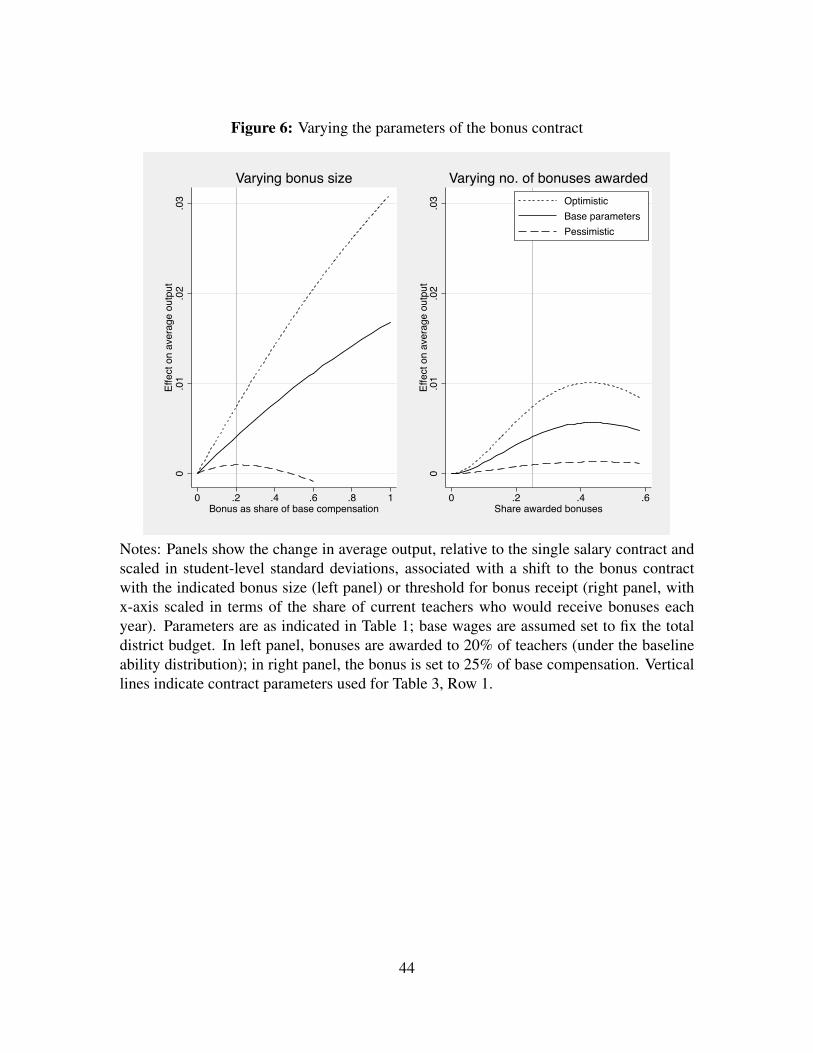
Figure 6: Varying the parameters of the bonus contract

0.0

1.0

2.0

3Ef

fect

on

aver

age

outp

ut

0 .2 .4 .6 .8 1Bonus as share of base compensation

Varying bonus size

0.0

1.0

2.0

3Ef

fect

on

aver

age

outp

ut

0 .2 .4 .6Share awarded bonuses

OptimisticBase parametersPessimistic

Varying no. of bonuses awarded

Notes: Panels show the change in average output, relative to the single salary contract andscaled in student-level standard deviations, associated with a shift to the bonus contractwith the indicated bonus size (left panel) or threshold for bonus receipt (right panel, withx-axis scaled in terms of the share of current teachers who would receive bonuses eachyear). Parameters are as indicated in Table 1; base wages are assumed set to fix the totaldistrict budget. In left panel, bonuses are awarded to 20% of teachers (under the baselineability distribution); in right panel, the bonus is set to 25% of base compensation. Verticallines indicate contract parameters used for Table 3, Row 1.

44

Figure 7: Varying the tenure rate and timing of tenure decisions

0.0

1.0

2.0

3.0

4Ef

fect

on

avg.

out

put

0 .2 .4 .6Fraction denied tenure

Base parameters

1 year2 years3 years4 years

Tenure decision after:

-.03

-.02

-.01

0.0

1Ef

fect

on

avg.

out

put

0 .2 .4 .6Fraction denied tenure

Pessimistic parameters

0.0

1.0

2.0

3.0

4Ef

fect

on

avg.

out

put

0 .2 .4 .6Fraction denied tenure

Optimistic parameters

Notes: Panels show the change in average output, relative to the single salary contract andscaled in student-level standard deviations, associated with a shift to the tenure contractwith the indicated tenure denial rate, using different decision dates and parameter values.Parameters are as indicated in Table 1; base wages are assumed set to fix the total districtbudget. Marked points indicate the contract parameters (20% denied tenure, with decisionsafter the second year) used for Table 3, Row 1.

45

Figure 8: Joint effects of tenure contracts and budget increases

0.0

1.0

2.0

3.0

4Ef

fect

on

avg.

out

put

0 .2 .4 .6Fraction denied tenure

Base parameters

Baseline budget5% budget increase

-.02

-.01

0.0

1.0

2Ef

fect

on

avg.

out

put

0 .2 .4 .6Fraction denied tenure

Pessimistic parameters

0.0

1.0

2.0

3.0

4.0

5.0

6Ef

fect

on

avg.

out

put

0 .2 .4 .6Fraction denied tenure

Optimistic parameters

Notes: Panels show changes in average output, relative to the single salary contract underthe baseline budget and scaled in student-level standard deviations, associated with alter-native tenure denial rates and/or budget allocations. Parameters are as indicated in Table 1;base wages are assumed set to fix the total district budget. Marked points indicate the con-tract parameters (20% denied tenure, with decisions after the second year) used for Table3, Row 1. Dashed line models a 5% budget increase.

46

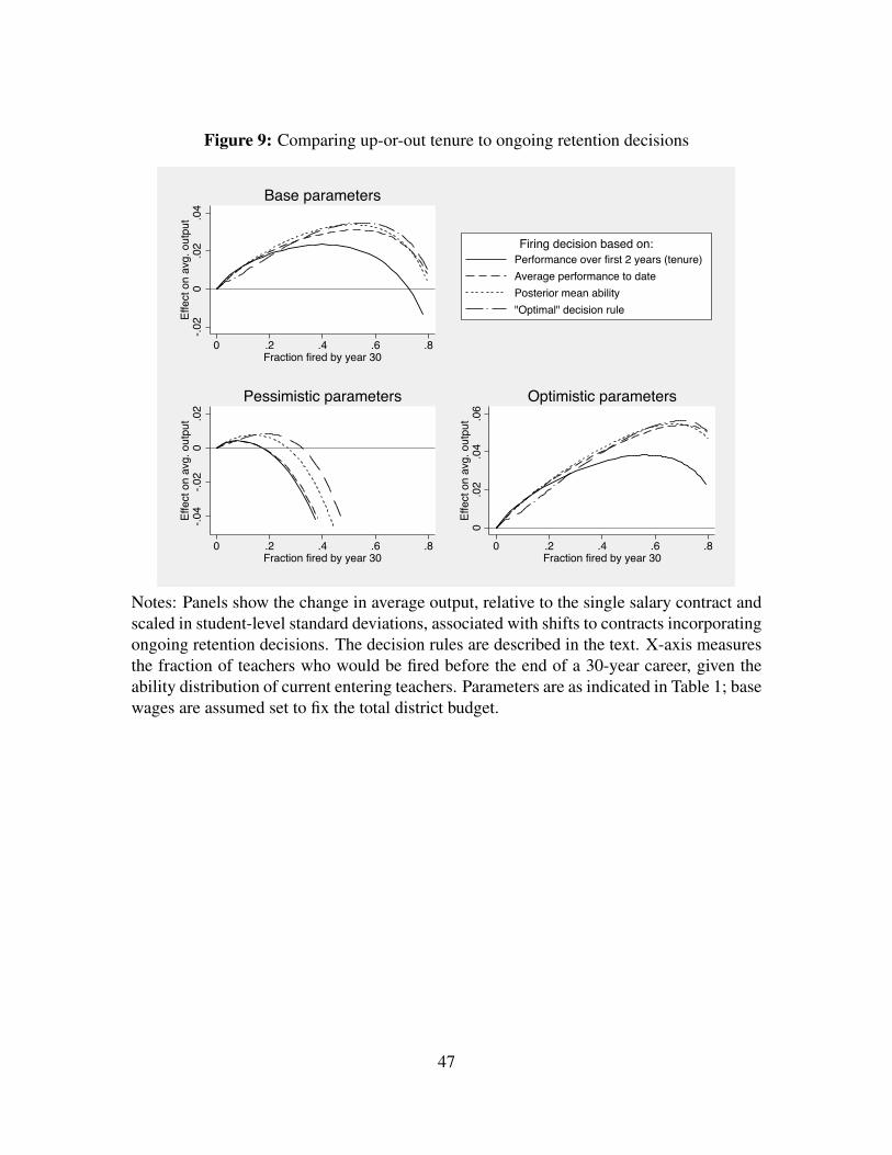
Figure 9: Comparing up-or-out tenure to ongoing retention decisions

-.02

0.0

2.0

4Ef

fect

on

avg.

out

put

0 .2 .4 .6 .8Fraction fired by year 30

Base parameters

Performance over first 2 years (tenure)Average performance to datePosterior mean ability"Optimal" decision rule

Firing decision based on:

-.04

-.02

0.0

2Ef

fect

on

avg.

out

put

0 .2 .4 .6 .8Fraction fired by year 30

Pessimistic parameters

0.0

2.0

4.0

6Ef

fect

on

avg.

out

put

0 .2 .4 .6 .8Fraction fired by year 30

Optimistic parameters

Notes: Panels show the change in average output, relative to the single salary contract andscaled in student-level standard deviations, associated with shifts to contracts incorporatingongoing retention decisions. The decision rules are described in the text. X-axis measuresthe fraction of teachers who would be fired before the end of a 30-year career, given theability distribution of current entering teachers. Parameters are as indicated in Table 1; basewages are assumed set to fix the total district budget.

47

Table 1: Values of key parameters

ParameterBaseline Pessimistic Optimistic

(1) (2) (3)Effectiveness

στ SD,of,teacher,ability

Υ Effect,of,1%,increase,in,class,size 70.004Measurement

σε SD,of,noise,in,annual,performanceTeacher,preferences,&,information

h Reliability,of,private,information 0.1 0.05 0.25δ Discount,rate 0.97u() von,Neumann7Morganstern,utility Linear CRRA,,ρ=3 Linearη Elasticity,of,entry,w.r.t.,w0 1 0.5 1.5

ζ Absolute,elasticity,of,exit,w.r.t.,w0 1 0.5 1.5

λ0 Annual,exit,hazard,,base,contract 0.08T Maximum,career,length 30κ Effect,of,being,fired 1%*,

min(t,10%)15% 1%*,

min(t,5%)Base,contract

g(t) Return,to,experienceBonus,contract

b Bonus,size,(as,share,of,base,pay)sB Share,of,teachers,receiving,bonusαB Base,pay,adjustment,(calibrated)

Fixed,quantity,scenario 73.5% 72.7% 73.5%Fixed,budget,scenario 73.5% 72.9% 73.5%

Tenure,contractsT Share,of,teachers,receiving,tenure 80%αT Base,pay,adjustment,(calibrated)

Fixed,quantity,scenario +12.6% +57.8% +8.5%Fixed,budget,scenario +10.4% +27.1% +7.4%

0,,,,,,,if,t>2

r(t)

0.18

20%25%

0.015*t

Experience,effect,on,productivity

Scenario

0.1570.07,if,t=070.04,if,t=170.02,if,t=2

48

Table 2: Impact of bonus and firing contracts on teacher effectiveness and total costs

BaselineBonuses Tenure Bonuses Tenure

(1) (2) (3) (4) (5)Outcomes)under)alternative)contracts

Number'of'teachers 1 1.00 1.00 1.00 0.97Teacher'ability'(τ)

Mean 0.000 0.004 0.033 0.004 0.033SD [0.150] [0.151] [0.135] [0.151] [0.135]

Teacher'experiencePct.'1st'year 8.0% 8.0% 8.9% 8.0% 9.0%Pct.'1st'3'years 30.9% 30.9% 31.1% 30.9% 31.6%Mean 8.82 8.83 9.09 8.83 8.99

Teacher'effectiveness'(τ+r(t))Mean L0.011 L0.007 0.021 L0.007 0.021SD [0.151] [0.153] [0.139] [0.153] [0.139]

Class'size'effect'(rel.'to'baseline) 0 0.000 0.000 0.000 L0.014Avg.'output'(teacher'effect'+'class'size) L0.011 L0.007 0.021 L0.007 0.007Salaries'(expressed'as'multiple'of'baseline'starting'salary)

Base'starting'salary 1.000 0.965 1.126 0.965 1.104Average'total'pay 1.148 1.147 1.298 1.147 1.271

Change)from)baselineNumber'of'teachers n/a n/a +0.01% L3.4%Teacher'ability'(τ)

Mean +0.004 +0.033 +0.004 +0.033SD +0.001 L0.015 +0.001 L0.015

Teacher'experiencePct.'1st'year L0.0'p.p. +0.8'p.p. L0.0'p.p. +1.0'p.p.

Pct.'1st'3'years L0.0'p.p. +0.3'p.p. L0.0'p.p. +0.7'p.p.Mean +0.009 +0.270 +0.009 +0.167

Teacher'effectiveness'(τ+r(t))Mean +0.004 +0.033 +0.004 +0.032SD +0.001 L0.012 +0.001 L0.012

Class'size'effect +0.000 L0.000 +0.000 L0.014Avg.'output'(teacher'effect'+'class'size) +0.004 +0.033 +0.004 +0.018Salaries

Base'starting'salary L3.5% +12.6% L3.5% +10.4%Average'total'pay L0.1% +15.0% L0.0% +12.3%

Inelastic:demand Fixed:budget

Notes: Simulations use baseline parameter values from Table 1, Column 1.

49

Table 3: Sensitivity of results to alternative parameters: Effects on teacher output (in stu-dent SDs)

RowBaseline Pessimistic/

AlternativeOptimistic/Alternative Baseline Pessimistic/

AlternativeOptimistic/Alternative

(1) (2) (3) (4) (5) (6)1 Baseline +0.004 +0.001 +0.007 +0.018 /0.003 +0.023Varying6private6information2 h=0.05 +0.004 +0.006 +0.018 +0.0223 h=0.25 +0.005 +0.001 +0.019 /0.000Less6noisy6performance6measure4 σε=0.12 +0.006 +0.001 +0.010 +0.023 +0.002 +0.028Varying6the6supply6elasticities5 η=0.5 +0.004 +0.006 +0.015 +0.0196 η=1.5 +0.004 +0.001 +0.020 +0.0047 ζ=0.5 +0.002 +0.004 +0.014 +0.0198 ζ=1.5 +0.006 +0.004 +0.021 +0.0159 ζ6declines6with6t +0.006 +0.004 +0.007 +0.020 +0.014 +0.02310 η6rises6with6μ +0.004 +0.001 +0.007 +0.018 +0.002 +0.022Other11 Risk6averse6(CRRA=3) +0.003 +0.005 +0.017 +0.02212 High6firing6cost6(κ6=6/0.15) +0.015 +0.02313 λ=6%6in6years61/4;63%6

thereafter +0.003 +0.000 +0.005 +0.018 /0.005 +0.023

Bonuses Tenure

Notes: Row 1 uses parameter values from Table 1. Each successive row changes oneparameter at a time, as indicated; entries where the alternative parameter matches thatused in Row 1 are suppressed. All simulations assume a fixed budget, as in Columns4-5 of Table 2. Table entries represent impacts of the alternative contracts on averageteacher productivity, in student-level standard deviations relative to the baseline contract,incorporating changes in ability, in experience, and in class size. In Row 9, z = 1.5 ⇤min(0, t). In Row 10, h = 1.01 + 0.0649(µ/sµ). This approximates the elasticity thatarises in a Roy model with corr (µ,w1) = 0.1.

50

Table 4: Effects of contracts with fixed costs of entry

No#entry#cost#in#baseline

Total#impact

Incremental#impact#of#performance#

contract(1) (2) (3)

Introduce*bonus*contract +0.004 +0.004Introduce*tenure*contract +0.018 +0.018Eliminate*entry*cost

No*other*changes +0.006and*introduce*bonus*contract +0.010 +0.004and*introduce*tenure*contract +0.025 +0.018

Entry#cost#in#baseline

Notes: All simulations assume a fixed district budget, as in Columns 4-5 of Table 2. Sim-ulations in Column 2, Rows 1-2 assume that entering teachers must pay a fixed entry costequal to w0, both under the baseline contract and under the alternatives. Table entries rep-resent impacts of the alternative contracts on average teacher productivity, in student-levelstandard deviations relative to the baseline contract (with a fixed entry cost in Column 2,but without one in Column 1), incorporating changes in ability, in experience, and in classsize.

51

Table 5: Optimal bonus and firing policies

Baseline Pessimistic Optimistic(1) (2) (3)

A.#Bonuses#based#on#two/year#moving#average#performanceVarying(bonus(size,(with(baseline(threshold

Bonus(size 100%* 21% 100%*Change(in(avg.(compensation +1.0% +0.5% +2.3%Change(in(output +0.017 +0.001 +0.031

Varying(threshold,(with(baseline(sizeFraction(awarded(bonus 43% 46% 43%Change(in(avg.(compensation +0.004% +1.0% +0.1%Change(in(output +0.006 +0.001 +0.010

B.#Tenure#policiesVarying(date(of(tenure(and(fraction(denied

Year(of(tenure(decision 3 5* 3Fraction(denied(tenure 41% 13% 57%Change(in(avg.(compensation +24% +10% +30%Change(in(output +0.024 +0.006 +0.038

Varying(fraction(denied,(fixing(decision(in(year(2Fraction(denied(tenure 40% 7% 56%Change(in(avg.(compensation +26% +8% +33%Change(in(output +0.023 +0.004 +0.038

C.#Ongoing#retention#decisionsBased(on(average(performance(to(date

Fraction(not(retained 52% 10% 71%Change(in(avg.(compensation +39% +11% +53%Change(in(output +0.031 +0.004 +0.054

Based(on(posterior(meanFraction(not(retained 52% 14% 67%Change(in(avg.(compensation +37% +11% +45%Change(in(output +0.034 +0.008 +0.055

Based(on(optimal((static)(decision(ruleFraction(not(retained 55% 18% 70%Change(in(avg.(compensation +36% +10% +47%Change(in(output +0.035 +0.008 +0.056

Notes: Asterisks represent boundary maxima – I do not consider bonuses larger than 100%of base pay or tenure decisions occurring after year 5. All simulations assume a fixeddistrict budget. Changes in average compensation include base salaries, bonuses, and ex-perience premia. Changes in output represent the net change in average productivity, instudent-level standard deviations, incorporating changes in ability, experience, and classsize. Both changes are relative to the baseline contract.

52

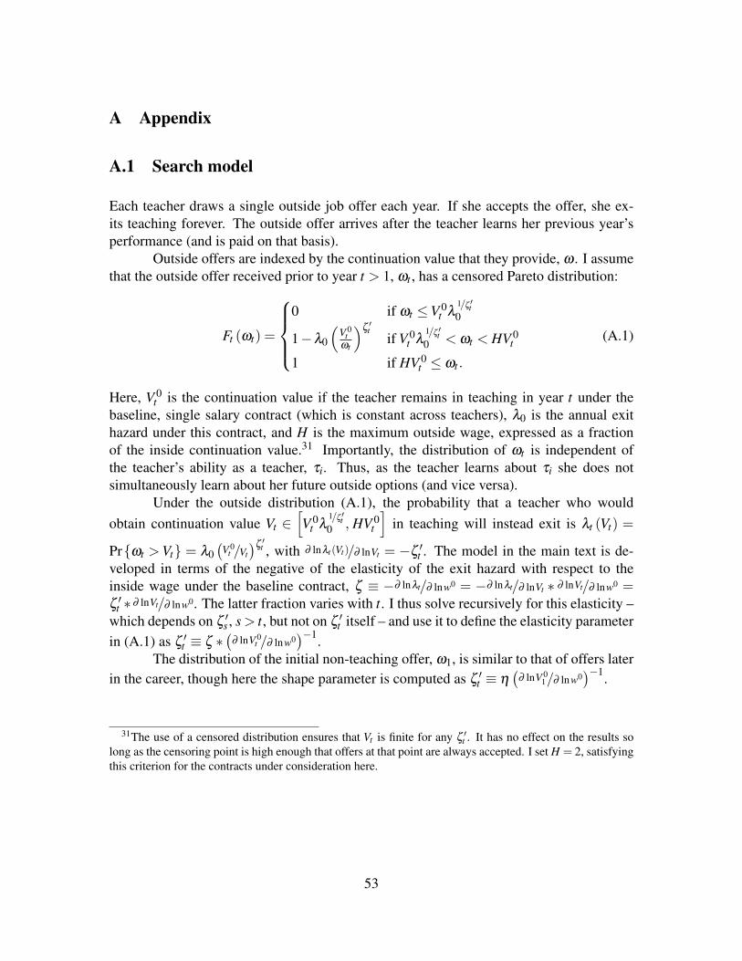
A Appendix

A.1 Search model

Each teacher draws a single outside job offer each year. If she accepts the offer, she ex-its teaching forever. The outside offer arrives after the teacher learns her previous year’sperformance (and is paid on that basis).

Outside offers are indexed by the continuation value that they provide, w . I assumethat the outside offer received prior to year t > 1, wt , has a censored Pareto distribution:

Ft (wt) =

8

>

>

<

>

>

:

0 if wt V 0t l 1/z 0t

0

1�l0

⇣

V 0t

wt

⌘z 0t

if V 0t l 1/z 0t

0 < wt < HV 0t

1 if HV 0t wt .

(A.1)

Here, V 0t is the continuation value if the teacher remains in teaching in year t under the

baseline, single salary contract (which is constant across teachers), l0 is the annual exithazard under this contract, and H is the maximum outside wage, expressed as a fractionof the inside continuation value.31 Importantly, the distribution of wt is independent ofthe teacher’s ability as a teacher, ti. Thus, as the teacher learns about ti she does notsimultaneously learn about her future outside options (and vice versa).

Under the outside distribution (A.1), the probability that a teacher who wouldobtain continuation value Vt 2

h

V 0t l 1/z 0t

0 , HV 0t

i

in teaching will instead exit is lt (Vt) =

Pr{wt >Vt} = l0�

V 0t /Vt

�z 0t , with ∂ lnlt(Vt)/∂ lnVt = �z 0

t . The model in the main text is de-veloped in terms of the negative of the elasticity of the exit hazard with respect to theinside wage under the baseline contract, z ⌘ �∂ lnlt/∂ lnw0 = �∂ lnlt/∂ lnVt ⇤ ∂ lnVt/∂ lnw0 =z 0

t ⇤ ∂ lnVt/∂ lnw0. The latter fraction varies with t. I thus solve recursively for this elasticity –which depends on z 0

s , s > t, but not on z 0t itself – and use it to define the elasticity parameter

in (A.1) as z 0t ⌘ z ⇤

�

∂ lnV 0t /∂ lnw0

��1.The distribution of the initial non-teaching offer, w1, is similar to that of offers later

in the career, though here the shape parameter is computed as z 0t ⌘ h

�

∂ lnV 01/∂ lnw0

��1.

31The use of a censored distribution ensures that Vt is finite for any z 0t . It has no effect on the results so

long as the censoring point is high enough that offers at that point are always accepted. I set H = 2, satisfyingthis criterion for the contracts under consideration here.

53

A.2 Solving the model

Equation (3) does not have a closed-form solution, but for any specified contract it can besolved recursively. Under the learning model developed above, the distribution of period-tperformance measure given qt�1 is

yt |qt�1 ⇠ N

0

@tt�1,1

1(1�h)s2

t+ t�1

s2e

+s2e

1

A . (A.2)

This is a univariate distribution that can easily be computed for any specified value of tt�1.Given tt�1 and yt , computation of tt is trivial.

The recursive solution thus has three steps. First, I compute wCT (y1, . . . , yT ), the

final period wage under contract C as a function of the performance signals to date. Second,I compute the value of remaining in teaching in period T , VT (qT�1; C), as a function ofqT�1, by integrating wC

T over the conditional distribution of yT given by (A.2). Third, foreach t < T , given estimates of Vt+1 (qt ; C) as a function of qt , I compute wC

t (y1, . . . , yt) asa function of yt and qt�1, then integrate each over the distribution of yt (and therefore ofqt) given qt�1 to obtain Vt (qt�1; C).

The state space qt is of dimension t +1, creating a dimensionality problem for ca-reers of reasonable length. Note, however, that each of the contracts considered above re-duces the state space for computation of wC

t from the t-dimensional distribution {y1, . . . , yt}to a one- or two-dimensional distribution: {yt�1, yt} for the bonus contract and {yt} forthe tenure and alternative firing contracts. Meanwhile, the teacher’s assessment of herown ability at the end of period t � 1 can be summarized either by the single variableti,t�1 or by the pair {µ, yt�1}. I can thus focus on state spaces of only two dimensions,qt�1 = {tt�1, yt�1} for the bonus contract or qt�1 = {µ, yt�1} for the tenure and firingcontracts. I approximate the joint distributions of these two-dimensional state variablesand yt with grids of 1493 points spaced to have equal probability mass.

Having computed Vt (qt�1,C) for each t, qt�1, and C, I simulate the impact of poli-cies by drawing potential teachers from the {µ, t} distribution, then drawing performancemeasures {y1, . . . , yT} for each. For each career, I compute qt�1 and Vt at each year t, anduse these to compute the effects of contract C on the probability of entering the professionand, conditional on entering, on surviving to year t. Note that I need not model the dis-tribution of {µ, t} in the population of potential teachers – under my constant elasticityassumptions, changes in the returns to teaching induce proportional changes in the amountof labor supplied to teaching by each type that do not depend on the number of people ofthat type in the population.

54

A.3 Market clearing

Alternative contracts may yield greater or lesser entry or persistence in aggregate. For ex-ample, adding performance bonuses without reducing base pay will yield more entry fromhigh-µ teachers and greater persistence of high-tt teachers, without offsetting reductionsfrom teachers with low µ or tt . Under each alternative contract, I compute the steady-statesize of the teacher workforce, assuming that the contract has been in place for at least Tyears and that the same number of entering teachers have been hired in each year.

I consider two scenarios for labor demand. First, I assume that the education systemwill require the same number of teachers under the alternative contracts as are requiredunder the baseline contract; where my computation yields a larger or smaller workforcethan in baseline, I assume that the base salary is adjusted upward or downward to yield theappropriate number of teachers. The aB and aF parameters listed for the “fixed quantity”scenaro in Table 1 are the adjustments required given the other parameters listed there;these are found via a numerical search algorithm. My second scenario assumes insteadthat the system’s total budget is fixed, so that increases in average teacher salaries must beoffset by reductions in the number of teachers (and therefore by increases in class size). The“fixed budget” scenario rows in Table 1 show the a parameters that balance the district’sbudget, given suitable changes in class size.

A.4 Optimal firing thresholds

In Section 5.2, I consider the optimal choice of thresholds (i.e., cutoff values of yt) forfiring teachers at each year t. I compute these thresholds as the solution to the district’sdynamic optimization problem, assuming that the district pays a cost of firing a teacher thatis proportional to the expected number of years remaining in the teacher’s career and thatthe district is myopic about potential labor supply responses. Specifically, let xt representthe number of years that a teacher with t years of experience can be expected to remain inteaching given an annual exit probability of l0 and certain retirement after year T . It canbe shown that

xt =1�l0

l0

⇣

1� (1�l0)T�t⌘

.

Let Wt�

yt ; c f ire� represent the value of retaining a teacher (i.e., offering her employmentfor the next year) after year t < T if her average performance to date is yt and the firing costis c f ire; let W0

�

c f ire� represent the value of hiring a new teacher from the baseline abilitydistribution; and let Zt

�

c f ire� ⌘ W0�

c f ire�� c f irext represent the value of firing a teacherafter year t. Then the continuation value of retaining a teacher after year t = T �1 is:

Wt

⇣

yt ;c f ire⌘

= l0W0

⇣

c f ire⌘

+(1�l0)⇣

ft yt + r(t +1)+dW0

⇣

c f ire⌘⌘

, (A.3)

55

where ft =s2

tt�1s2

e +stand thus E [t|yt ] = ft yt . (d is the discount rate.) The continuation

value of retaining a teacher after year t < T �1 is:

Wt

⇣

yt ;c f ire⌘

= l0W0

⇣

c f ire⌘

+(1�l0)⇣

ft yt + r(t +1) (A.4)

+dEh

maxn

Wt+1

⇣

yt+1;c f ire⌘

,Zt+1

⇣

c f ire⌘o

�

�

�

yt

i⌘

,

Thus, the value of hiring a new teacher must be

W0

⇣

c f ire⌘

= 0+ r(0)+dEh

maxn

W1

⇣

y1;c f ire⌘

,Zt

⇣

c f ire⌘oi

. (A.5)

Given a choice of c f ire and a hypothesized value for W0, one can use (A.3), (A.4),and (A.5) recursively to solve for the implied value of W0. The fixed point for this is thevalue W0

�

c f ire�. Moreover, the firing thresholds at year t are the values of yt that equateWt�

yt ;c f ire�with Zt�

c f ire�, and these can be used to compute the share of entering teacherswho will be fired at some point in their careers. The estimates in Figure 9 are obtainedby choosing a range of values for c f ire; using a numerical search algorithm to find thefixed point W0 given c f ire; computing the firing thresholds implied by these values and theresulting firing shares; and then solving the labor supply model given these thresholds forthe market-clearing wages and average productivity levels.

56

Figure A.1: Empirical one-year attrition hazards from the 1999/00 Schools and StaffingSurvey/Teacher Follow-Up Survey

0.1

.2.3

Attri

tion

rate

0 10 20 30 40Years of experience

All exits from classroomExclude family leave, administration

Notes: Solid line shows fraction of teachers at each experience level in the 1999-2000Schools and Staffing Survey who are not teaching at the time of the one-year TeacherFollow-Up Survey. Dashed line codes as non-exits (a) individuals caring for family mem-bers at the time of the follow-up who say they plan to return to teaching within a year and(b) individuals who continue to work for state & local governments in non-teaching jobs inelementary and secondary education (e.g., as principals). Vertical line corresponds to theassumed retirement date (T = 30) used in simulations here. Horizontal lines correspondto the assumed annual attrition hazards used in the main (solid line; l = 0.08) simulationsand in the alternative simulation in Table 3, Row 13 (dotted line; l = 0.06 for experience< 5 and l = 0.03 thereafter). Sample sizes average 122 teachers per year of experiencebelow 30.

57

Figure A.2: Probability of ever being fired over a 30-year career under different decisionrules, by true ability

0.2

.4.6

.81

Frac

tion

ever

fire

d

0 10 20 30 40 50 60 70 80 90 100Percentile of true ability

TenureFire - Avg. performanceFire - Posterior meanFire - Optimal decision rule

Notes: See Section 5.3 for description of the decision rules. Each rule is set so that, giventhe current ability distribution, the unconditional probability of being fired before the endof a 30 year career, equals 20%. Figure shows probabilities conditional on ability, t .

58

Figure A.3: Cumulative firing probability by true ability decile and experience under dif-ferent decision rules

0.5

10

.51

0 10 20 30 0 10 20 30

Lowest decile Second decile

Third and fourth deciles Deciles five to ten

Tenure Fire - Avg. performanceFire - Posterior mean Fire - Optimal decision rule

Cum

ulat

ive fr

actio

n fir

ed

Years of experience

Graphs by ability group

Notes: See Section 5.3 for description of the decision rules. Each rule is set so that, giventhe current ability distribution, the unconditional probability of being fired before the endof a 30 year career, equals 20%. Figure shows the probability that a teacher will be fired onor before year t under each decision rule, given ability in the indicated group and assumingno voluntary exit.

59