Teaching Economics Interactively: A Cannibal’s Dinner Party

Hillsdale College Free Market Forum

Ted Bergstrom, UCSB

What I tell my Principles Students

• “Taking this course is like being invited to dinner at a cannibal’s house. ‘’

• ``You may be a diner, you may be dinner…

• And you probably will be both’’

A Cannibal’s Feast

• Unlike astronomers, physicists, geologists,

botanists, or even biologists, we have direct experience with being the object we study.

• ``Economics is the study of mankind in the ordinary business of life.’’---Alfred Marshall

• The classroom is a natural laboratory for study of interacting human decisions…as well as a place to learn economics.

Two Interactive Devices

• Classroom Market Experiments in TA Sections.

• Radio Frequency Clickers in large lectures.

Principles class has 500+ students. Sections have 35-50.

Classroom Experiments

• Each week students participate in a market experiment in the TA section.

• Experiment illustrates economic principles studied in that week.

• Each student’s trades and profits are recorded. (Profits count slightly toward grade.)

• Data from experiment is posted on web. • Homework assignment: Process data from

experiment and compare experimental results with theoretical predictions.

Classroom lectures

• In large lecture we discuss the theory related to the experiment.

• We see how well the theory predicts experimental results.

• Important lesson: Distinguish Predictions from observations.

• We look at real world ``natural experiments’’ that illustrate the theory.

Pedagogical objectives

Persuade students that economics is not dogma to memorize, but tools for thinking about what goes on in the world.

Teach them the usefulness of simple theories and the difference between theory and observation.

Experimental topics

• Demand and Supply (and shifts in these)

• Sales tax incidence

• Price Floors and Ceilings

• Externalities

• Equilibrium with entry and exit of firms

• Monopoly and Oligopoly

• Comparative Advantage

• Adverse Selection and Lemons

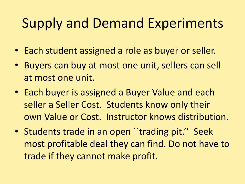
Supply and Demand Experiments

• Each student assigned a role as buyer or seller.

• Buyers can buy at most one unit, sellers can sell at most one unit.

• Each buyer is assigned a Buyer Value and each seller a Seller Cost. Students know only their own Value or Cost. Instructor knows distribution.

• Students trade in an open ``trading pit.’’ Seek most profitable deal they can find. Do not have to trade if they cannot make profit.

Theoretical Prediction

• After experiment is over, students are told the distribution of Buyer Values and Seller Costs.

• They are asked to construct a supply curve and a demand curve and to find the competitive equilibrium price.

• In homework, they compare the prices and quantities in the experimental outcome to the predictions of competitive theory.

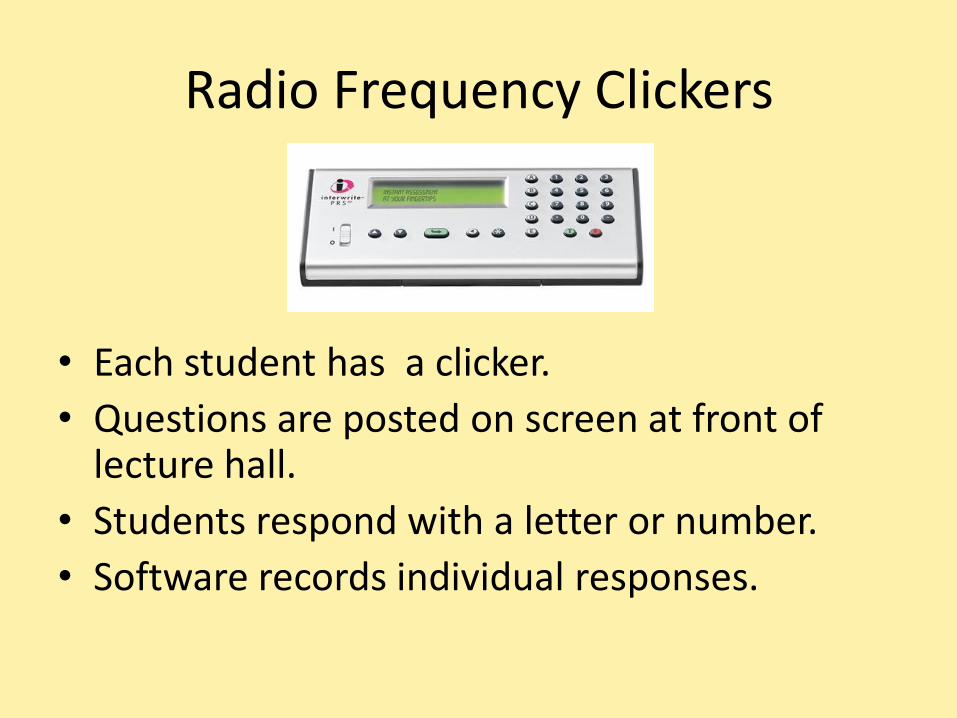
Radio Frequency Clickers

• Each student has a clicker.

• Questions are posted on screen at front of lecture hall.

• Students respond with a letter or number.

• Software records individual responses.

Clicker Applications

• Surveys of characteristics or opinions

– Develop demand and supply curves to work with as homework exercises

• Questions testing understanding of material

– Inform me of what students know

– Inform students of what I want them to know

– Inform students of what the others know.

• Classroom games and markets

Survey Questions

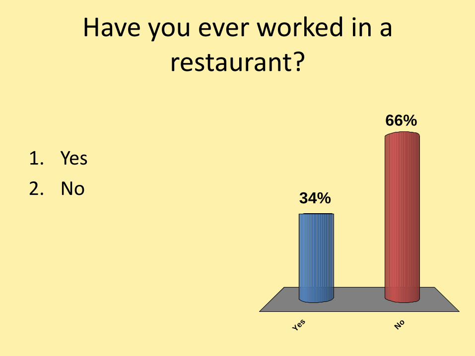
Have you ever worked in a restaurant?

Yes N

o

66%

34%

1. Yes

2. No

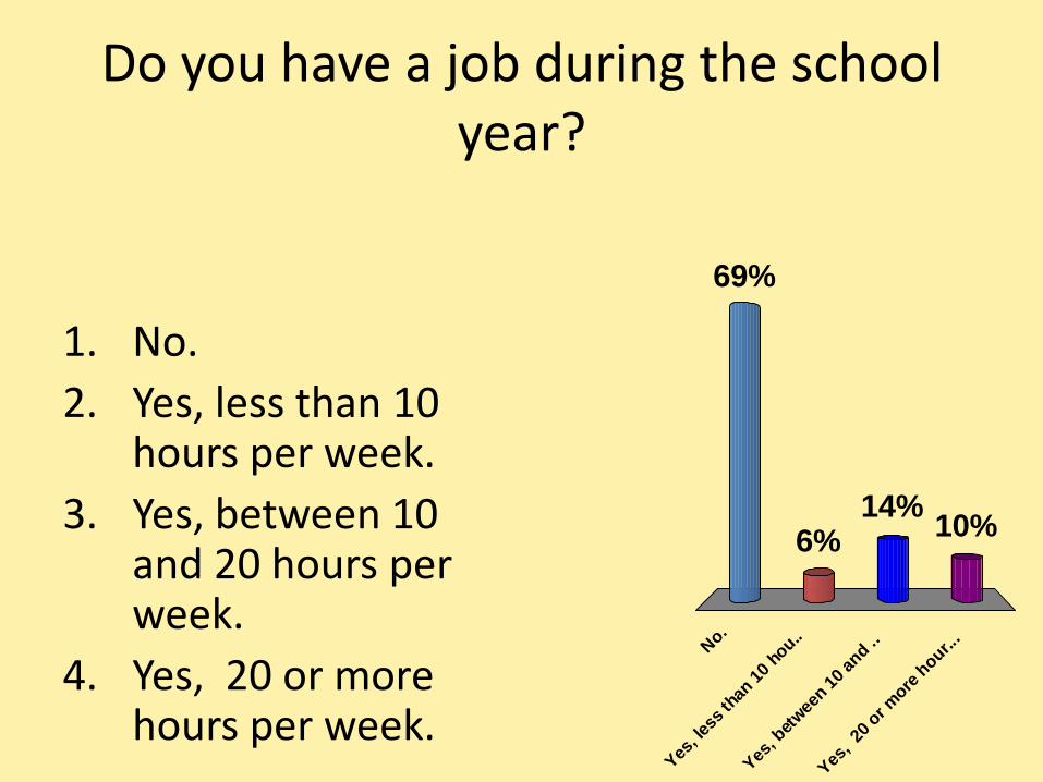
Do you have a job during the school year?

1. No.

2. Yes, less than 10 hours per week.

3. Yes, between 10 and 20 hours per week.

4. Yes, 20 or more hours per week.

No.

Yes

, les

s th

an 1

0 ho

u..

Yes

, bet

wee

n 10

and ..

Yes

, 20

or m

ore h

our...

69%

10%14%

6%

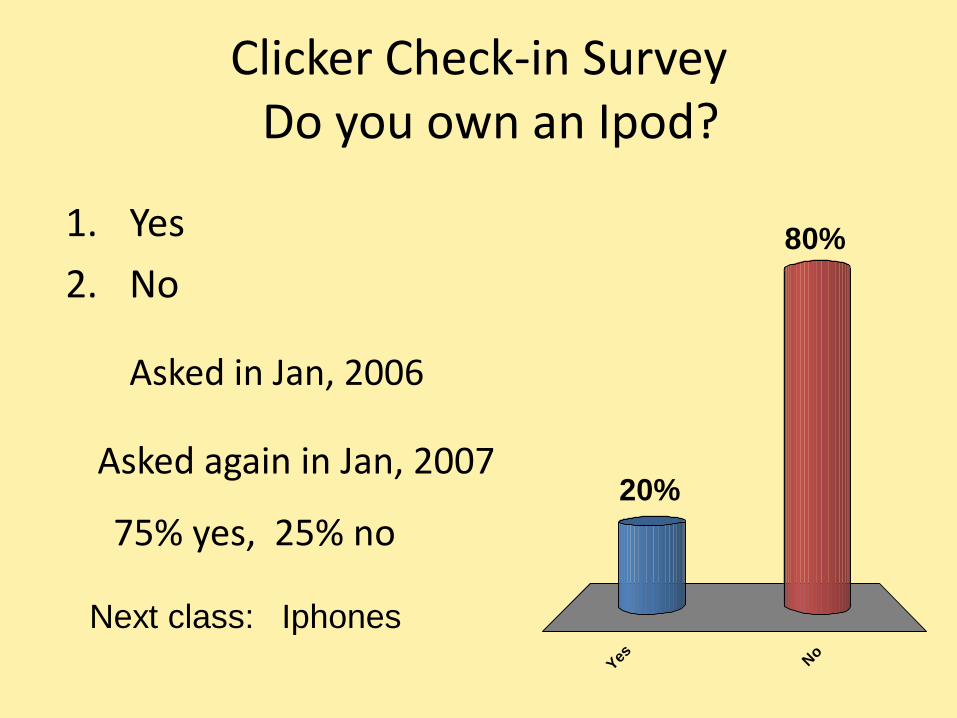
Clicker Check-in SurveyDo you own an Ipod?

Yes N

o

80%

20%

1. Yes

2. No

Asked in Jan, 2006

Asked again in Jan, 2007

75% yes, 25% no

Next class: Iphones

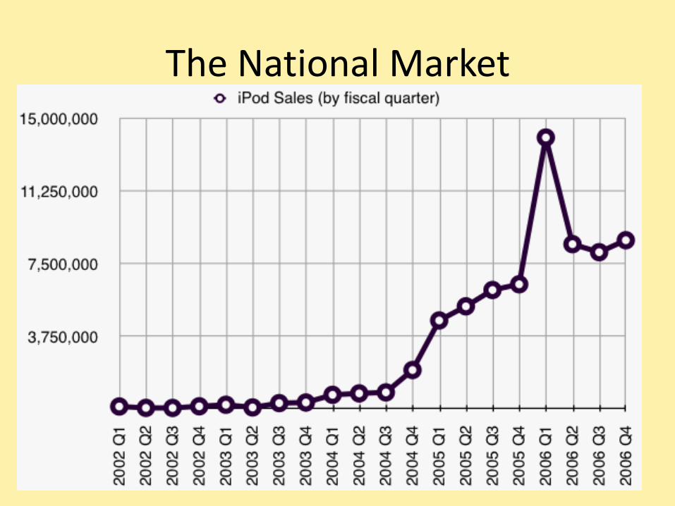
The National Market

Estimating a Demand Function

Question:

What is the most that would you be willing to pay for an IPOD if you couldn’t get it any cheaper than that?

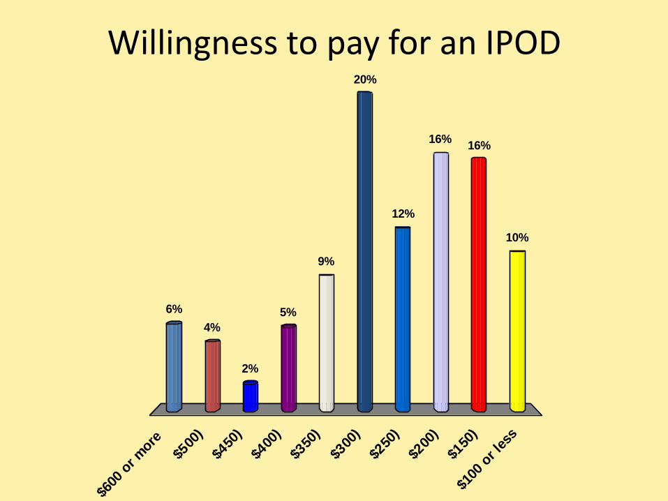
Willingness to pay for an IPOD

$60

0 or m

ore

$500

)

$450

)

$400

)

$350

)

$300

)

$250

)

$200

)

$150

)

$10

0 or le

ss

6%

4%

2%

5%

10%

16%16%

12%

20%

9%

Homework assignment

• Students were given an Excel spreadsheet with the distribution of willingnesses to pay.

• They were told that I would ask the following clicker questions in class next time.

What price maximizes revenue?

If marginal cost is $50, what price maximizes profit?

If marginal cost is $100, what price maximizes profit?

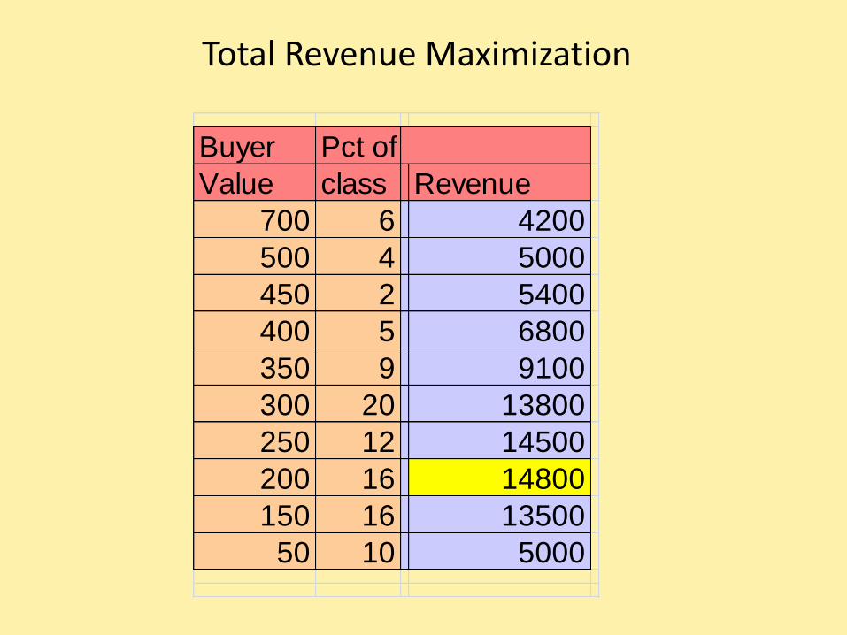
Total Revenue Maximization

Buyer Pct of

Value class Revenue

700 6 4200

500 4 5000

450 2 5400

400 5 6800

350 9 9100

300 20 13800

250 12 14500

200 16 14800

150 16 13500

50 10 5000

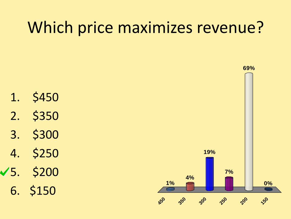
Which price maximizes revenue?

450

350

300

250

200

150

1%4%

0%

69%

7%

19%

1. $450

2. $350

3. $300

4. $250

5. $200

6. $150

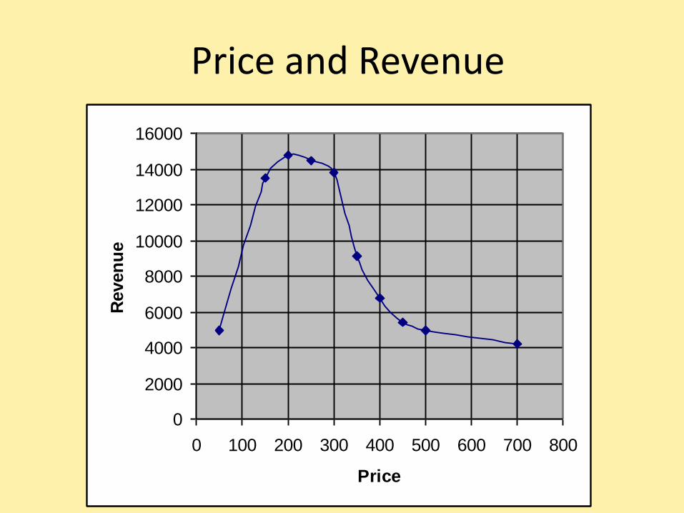
Price and Revenue

0

2000

4000

6000

8000

10000

12000

14000

16000

0 100 200 300 400 500 600 700 800

Price

Reven

ue

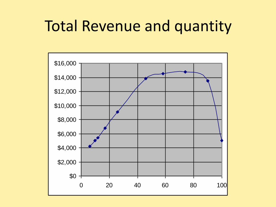
Total Revenue and quantity

$0

$2,000

$4,000

$6,000

$8,000

$10,000

$12,000

$14,000

$16,000

0 20 40 60 80 100

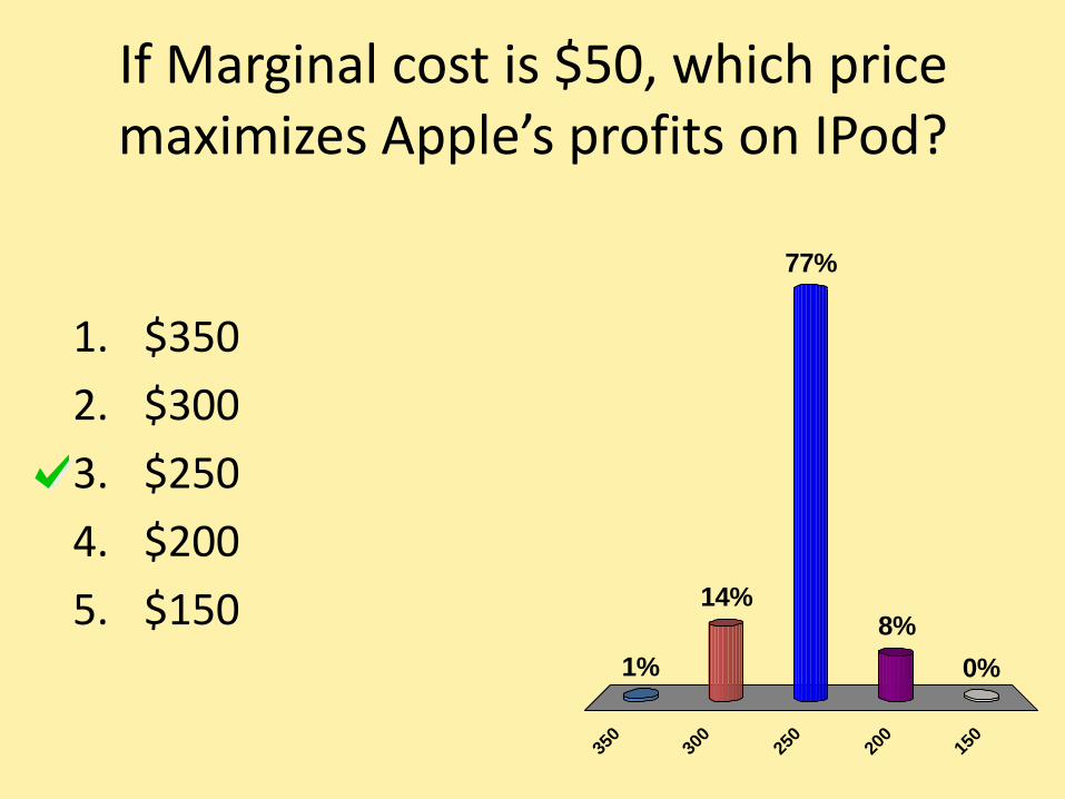
If Marginal cost is $50, which price maximizes Apple’s profits on IPod?

350

300

250

200

150

1%

14%

0%

8%

77%

1. $350

2. $300

3. $250

4. $200

5. $150

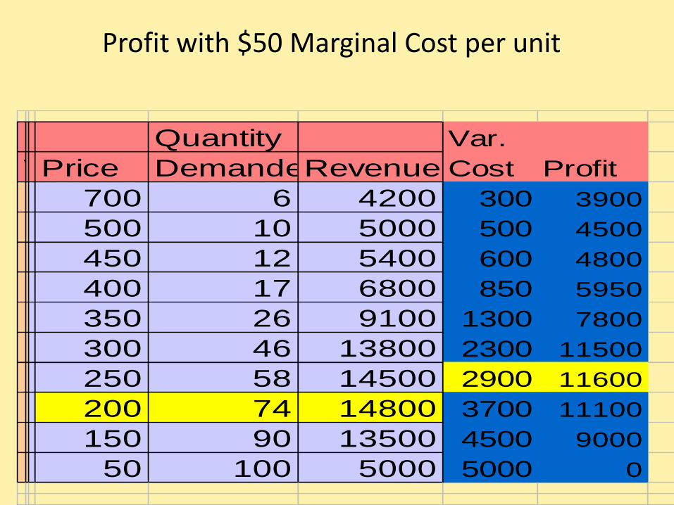
Profit with $50 Marginal Cost per unit

BuyerPct of Quantity Var.

Valueclass Price DemandedRevenue Cost Profit

700 6 4200 300 3900

500 10 5000 500 4500

450 12 5400 600 4800

400 17 6800 850 5950

350 26 9100 1300 7800

300 46 13800 2300 11500

250 58 14500 2900 11600

200 74 14800 3700 11100

150 90 13500 4500 9000

50 100 5000 5000 0

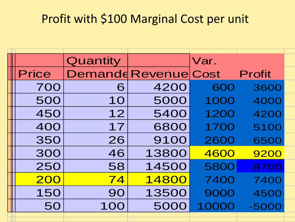
Profit with $100 Marginal Cost per unit

BuyerPct of Quantity Var.

Valueclass Price DemandedRevenue Cost Profit

700 6 4200 600 3600

500 10 5000 1000 4000

450 12 5400 1200 4200

400 17 6800 1700 5100

350 26 9100 2600 6500

300 46 13800 4600 9200

250 58 14500 5800 8700

200 74 14800 7400 7400

150 90 13500 9000 4500

50 100 5000 10000 -5000

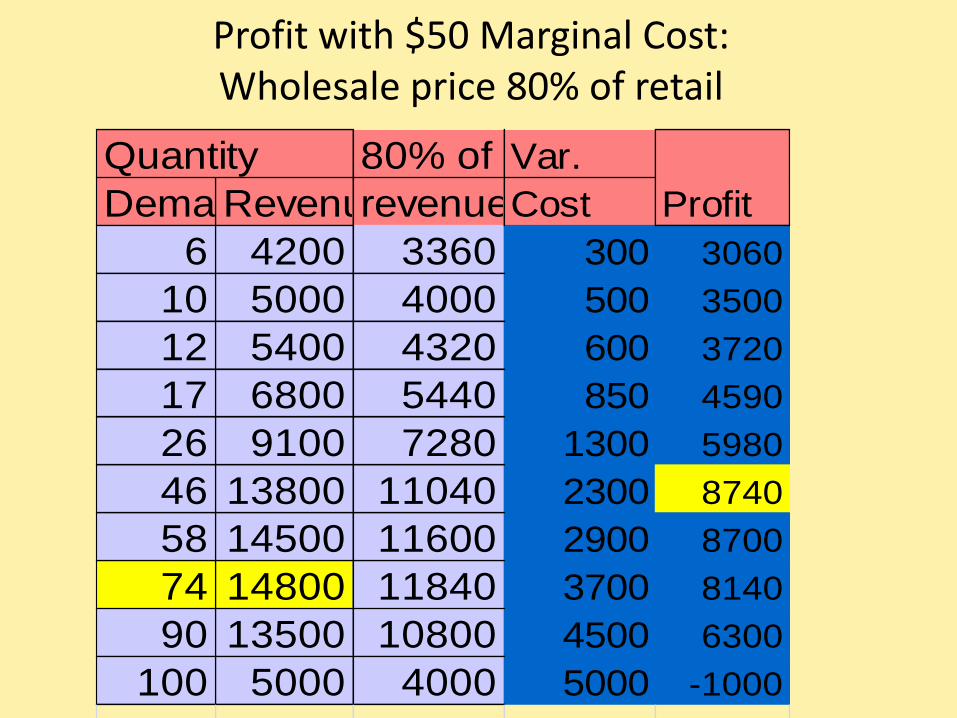
Profit with $50 Marginal Cost:Wholesale price 80% of retail

Quantity 80% of Var.

DemandedRevenuerevenueCost Profit

6 4200 3360 300 3060

10 5000 4000 500 3500

12 5400 4320 600 3720

17 6800 5440 850 4590

26 9100 7280 1300 5980

46 13800 11040 2300 8740

58 14500 11600 2900 8700

74 14800 11840 3700 8140

90 13500 10800 4500 6300

100 5000 4000 5000 -1000

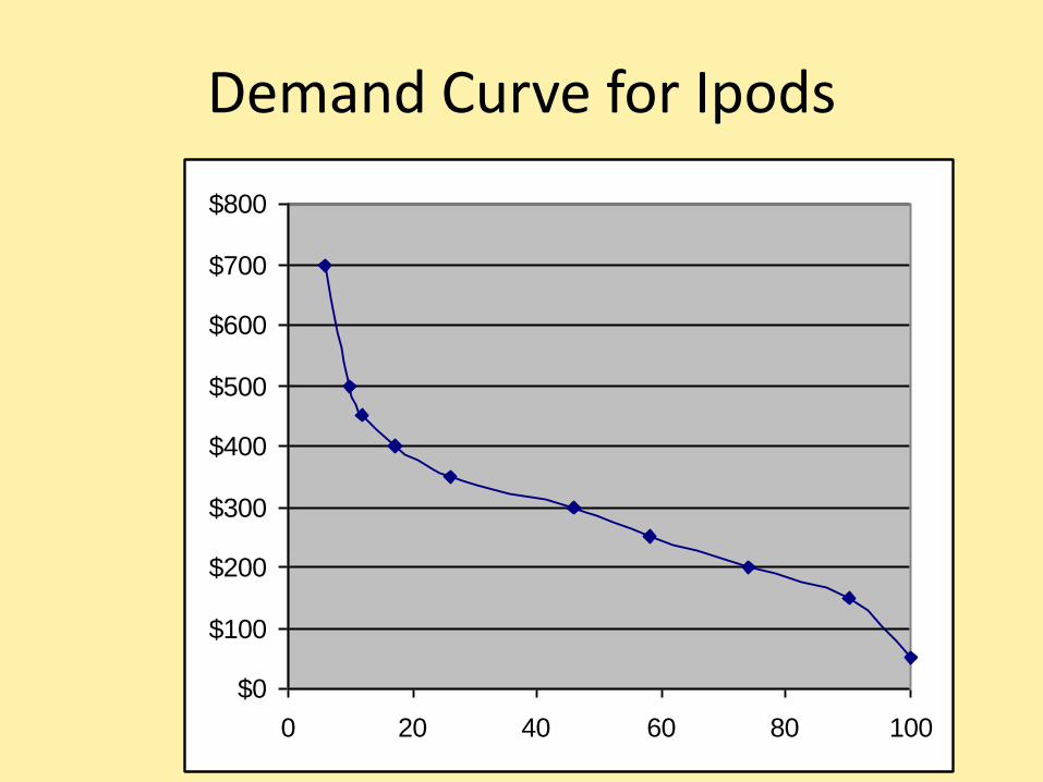
Demand Curve for Ipods

$0

$100

$200

$300

$400

$500

$600

$700

$800

0 20 40 60 80 100

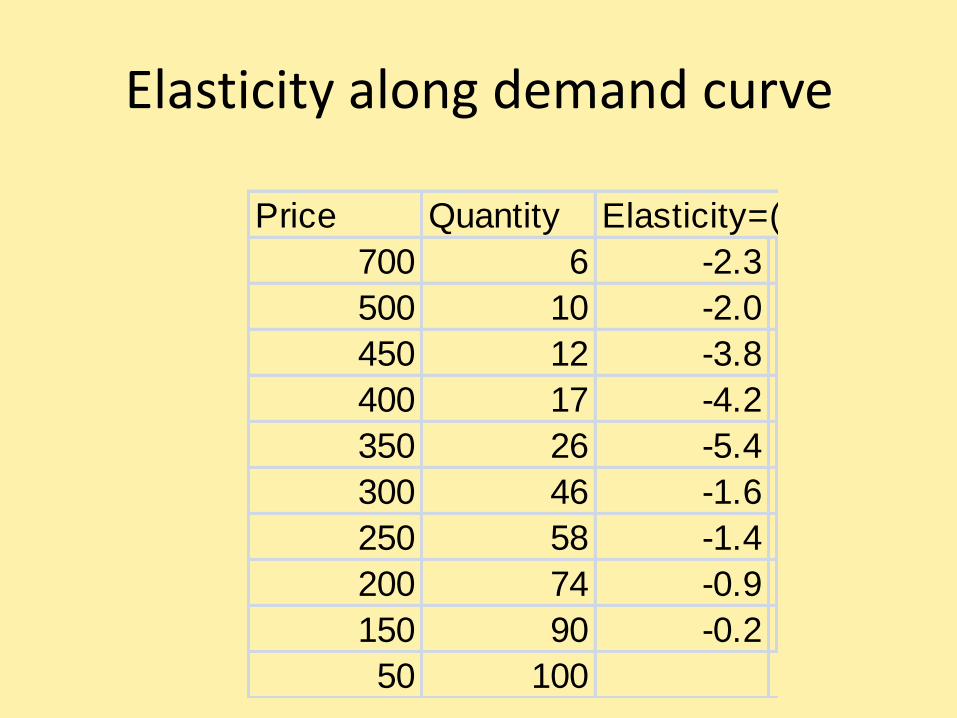
Elasticity along demand curve

Price Quantity Elasticity=(P/Q)(DQ/DP)

700 6 -2.3

500 10 -2.0

450 12 -3.8

400 17 -4.2

350 26 -5.4

300 46 -1.6

250 58 -1.4

200 74 -0.9

150 90 -0.2

50 100

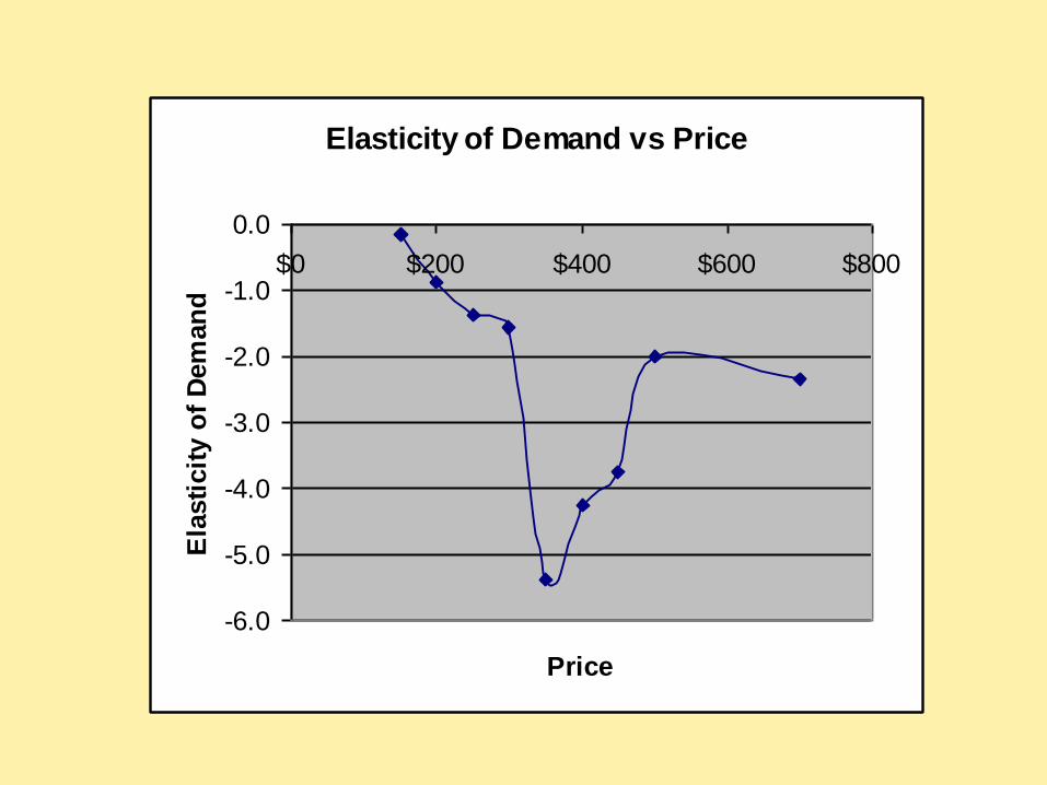
Elasticity of Demand vs Price

-6.0

-5.0

-4.0

-3.0

-2.0

-1.0

0.0

$0 $200 $400 $600 $800

Price

Ela

sti

cit

y o

f D

em

an

d

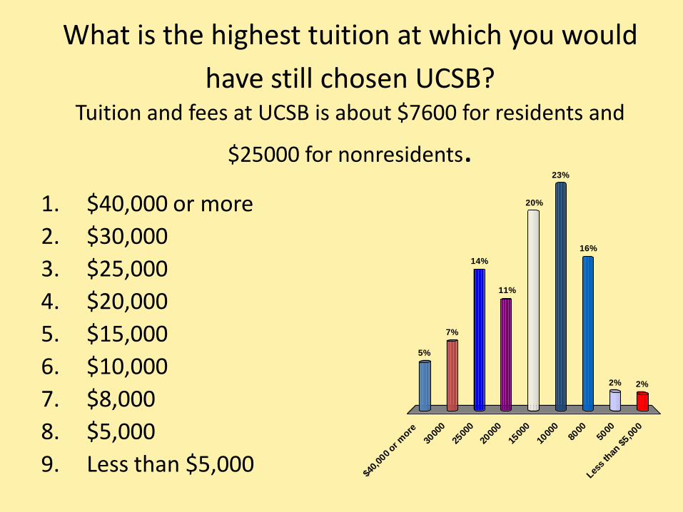
What is the highest tuition at which you would

have still chosen UCSB? Tuition and fees at UCSB is about $7600 for residents and

$25000 for nonresidents.

$40

,000

or m

ore

3000

0

2500

0

2000

0

1500

0

1000

0

8000

5000

Les

s th

an $

5,000

5%

7%

14%

11%

2%2%

16%

23%

20%1. $40,000 or more

2. $30,000

3. $25,000

4. $20,000

5. $15,000

6. $10,000

7. $8,000

8. $5,000

9. Less than $5,000

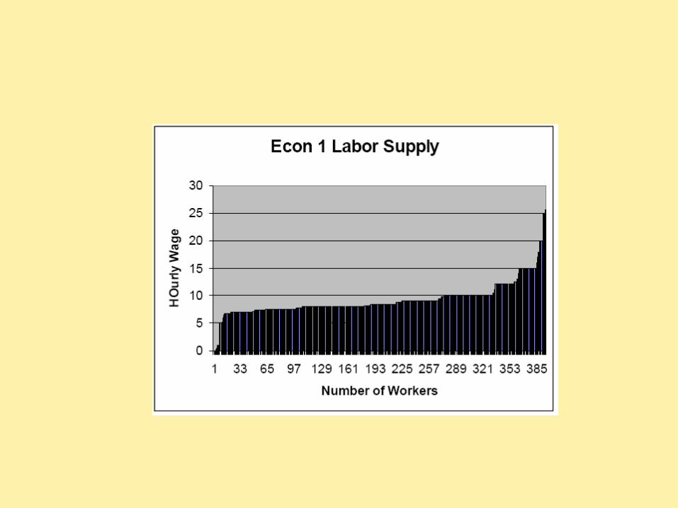
Labor Supply Question

• What is the lowest hourly wage at which you would take a 10 hour per week part time job during the school year?

Questions on Course Material

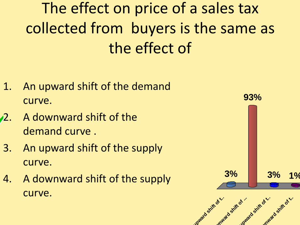
The effect on price of a sales tax collected from buyers is the same as

the effect of

1. An upward shift of the demand curve.

2. A downward shift of the demand curve .

3. An upward shift of the supply curve.

4. A downward shift of the supply curve.

An u

pwar

d shift

of t

..

A d

ownw

ard

shift

of .

..

An u

pwar

d shift

of t

..

A d

ownw

ard

shift

of t

..

3% 1%3%

93%

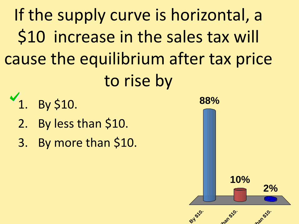
If the supply curve is horizontal, a $10 increase in the sales tax will

cause the equilibrium after tax price to rise by

By

$10.

By

less

than

$10

.

By

mor

e th

an $

10.

88%

2%10%

1. By $10.

2. By less than $10.

3. By more than $10.

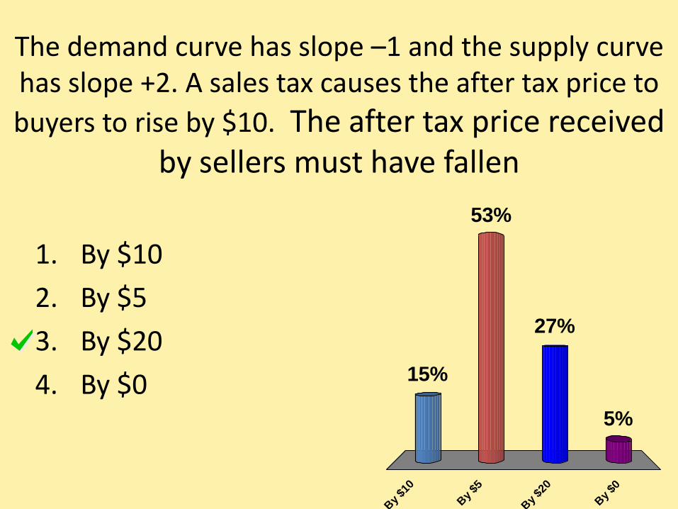
The demand curve has slope –1 and the supply curve has slope +2. A sales tax causes the after tax price to

buyers to rise by $10. The after tax price received by sellers must have fallen

1. By $10

2. By $5

3. By $20

4. By $0

By

$10

By

$5

By

$20

By

$0

15%

5%

27%

53%

Looking pretty good

• Maybe they are learning something.

• Let’s try another one.

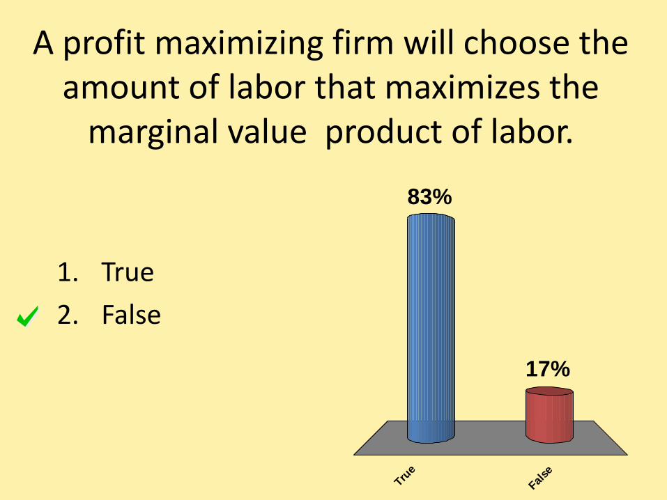
A profit maximizing firm will choose the amount of labor that maximizes the

marginal value product of labor.

Tru

e

Fal

se

17%

83%

1. True

2. False

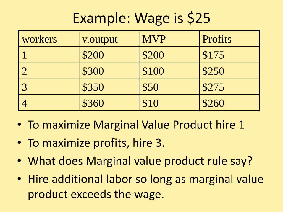
• To maximize Marginal Value Product hire 1

• To maximize profits, hire 3.

• What does Marginal value product rule say?

• Hire additional labor so long as marginal value product exceeds the wage.

workers v.output MVP Profits

1 $200 $200 $175

2 $300 $100 $250

3 $350 $50 $275

4 $360 $10 $260

Example: Wage is $25

Worse than a roomful of monkeys?

• If you want to deflate your opinion of your teaching prowess, ask your students a variant of this question.

– Monopolists seek to maximize their marginal revenue or

– Competitive firms seek to maximize the difference between price and marginal cost.

• Students are not used to careful use of language.

Classroom Games

A commuting game.

• You have two ways to commute from home to work. – The short way by narrow road

– The long way by freeway

• Commute time by freeway is always 30 minutes.

• Commute time by narrow road depends on how many others take narrow road.

Your choice

• If N people go short way, it takes 15+N/10 minutes to make the trip.

• Freeway always takes 30 minutes

• You hate commuting and want to minimize

travel time.

• Choose your route using Clickers. We’ll do this repeatedly, simulating commuter days.

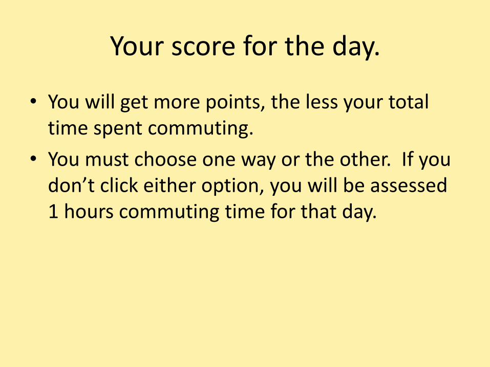
Your score for the day.

• You will get more points, the less your total time spent commuting.

• You must choose one way or the other. If you don’t click either option, you will be assessed 1 hours commuting time for that day.

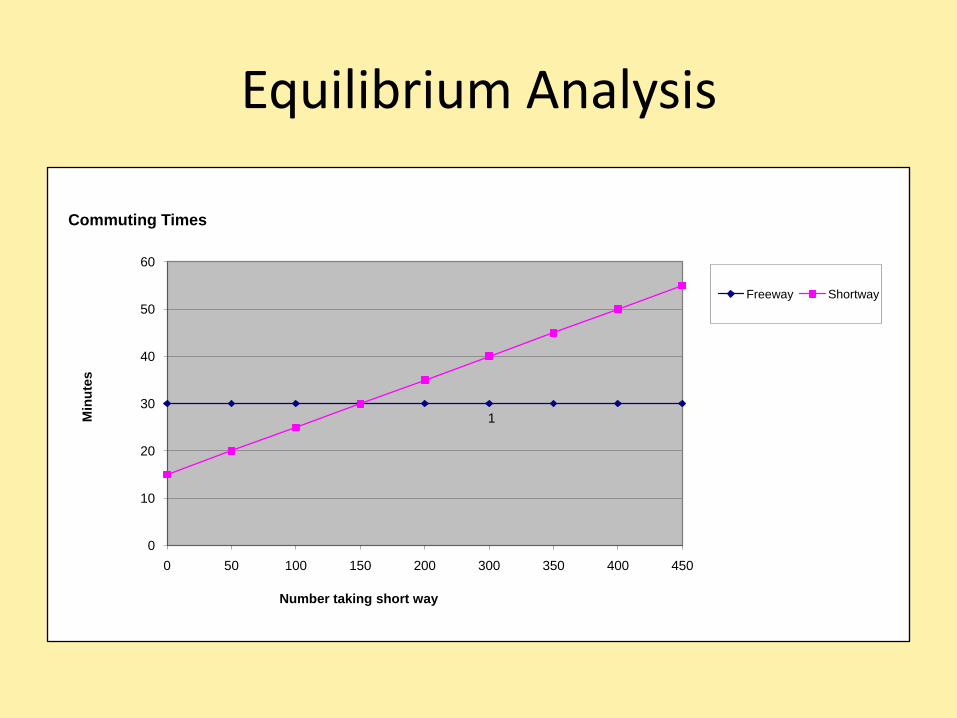
Equilibrium Analysis

0

10

20

30

40

50

60

0 50 100 150 200 300 350 400 450

Min

ute

s

Number taking short way

Commuting Times

Freeway Shortway

1

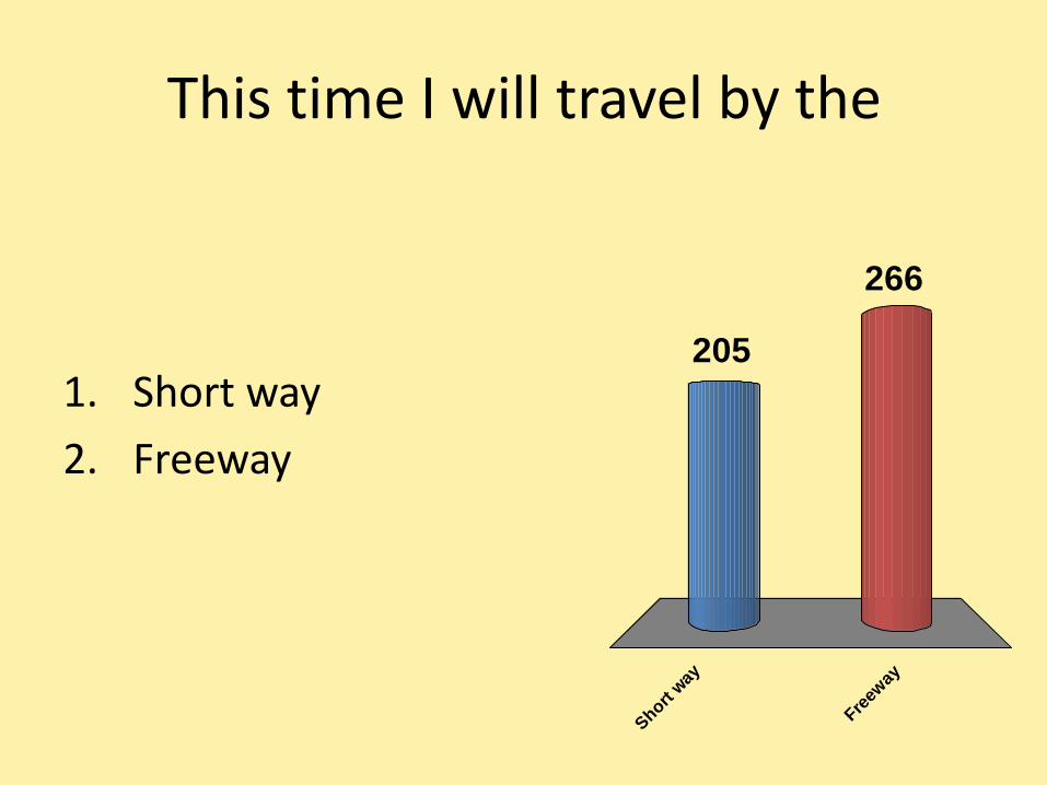
This time I will travel by the

1. Short way

2. Freeway

Short

way

Fre

eway

266

205

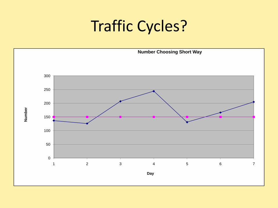
Traffic Cycles?

0

50

100

150

200

250

300

1 2 3 4 5 6 7

Nu

mb

er

Day

Number Choosing Short Way

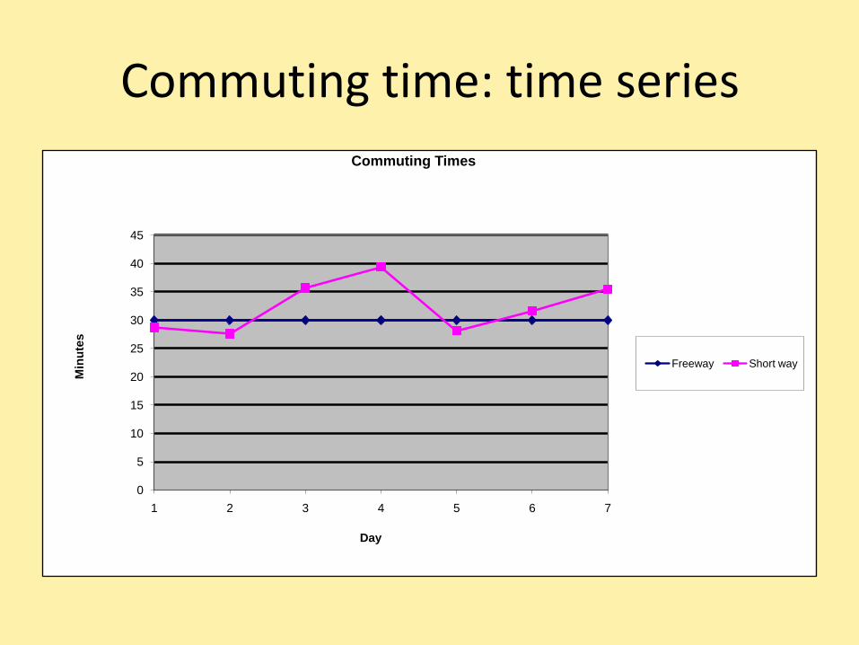
Commuting time: time series

0

5

10

15

20

25

30

35

40

45

1 2 3 4 5 6 7

Min

ute

s

Day

Commuting Times

Freeway Short way

The wisdom of Crowds?

• We can ask a question repeatedly, displaying the histogram of answers after each set of responses.

• How useful is group consensus about facts?

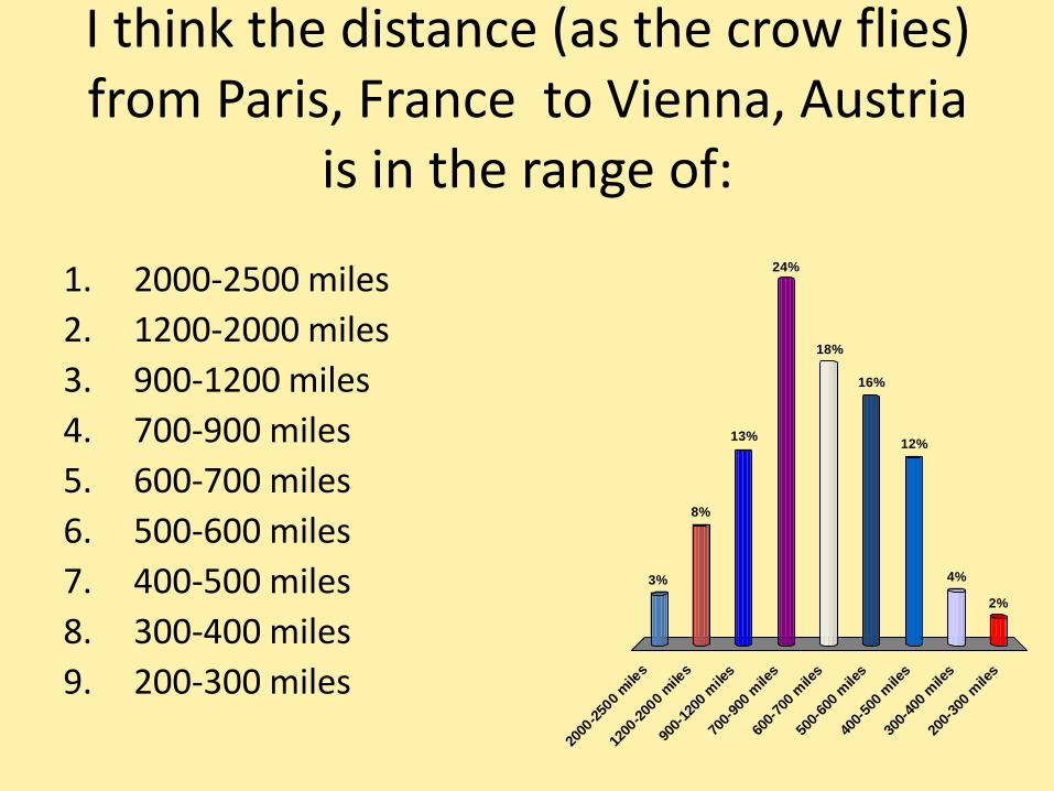
I think the distance (as the crow flies) from Paris, France to Vienna, Austria

is in the range of:

200

0-250

0 m

iles

120

0-200

0 m

iles

900

-120

0 mile

s

700

-900

mile

s

600

-700

mile

s

500

-600

mile

s

400

-500

mile

s

300

-400

mile

s

200

-300

mile

s

3%

8%

13%

24%

2%

4%

12%

16%

18%

1. 2000-2500 miles

2. 1200-2000 miles

3. 900-1200 miles

4. 700-900 miles

5. 600-700 miles

6. 500-600 miles

7. 400-500 miles

8. 300-400 miles

9. 200-300 miles

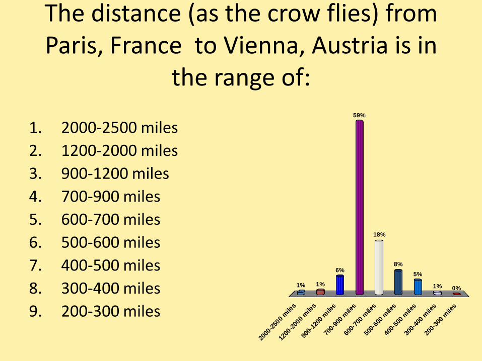
The distance (as the crow flies) from Paris, France to Vienna, Austria is in

the range of:

200

0-250

0 m

iles

120

0-200

0 m

iles

900

-120

0 mile

s

700

-900

mile

s

600

-700

mile

s

500

-600

mile

s

400

-500

mile

s

300

-400

mile

s

200

-300

mile

s

1% 1%

6%

59%

0%1%

5%

8%

18%

1. 2000-2500 miles

2. 1200-2000 miles

3. 900-1200 miles

4. 700-900 miles

5. 600-700 miles

6. 500-600 miles

7. 400-500 miles

8. 300-400 miles

9. 200-300 miles

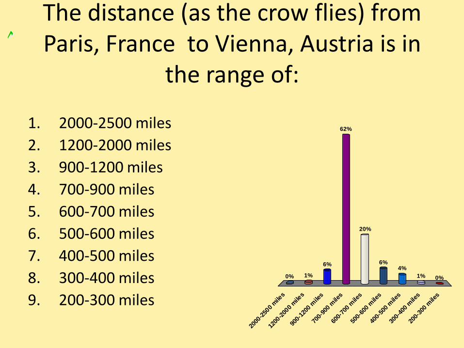
The distance (as the crow flies) from Paris, France to Vienna, Austria is in

the range of:

200

0-250

0 m

iles

120

0-200

0 m

iles

900

-120

0 mile

s

700

-900

mile

s

600

-700

mile

s

500

-600

mile

s

400

-500

mile

s

300

-400

mile

s

200

-300

mile

s

0% 1%

6%

62%

0%1%

4%6%

20%

1. 2000-2500 miles

2. 1200-2000 miles

3. 900-1200 miles

4. 700-900 miles

5. 600-700 miles

6. 500-600 miles

7. 400-500 miles

8. 300-400 miles

9. 200-300 miles

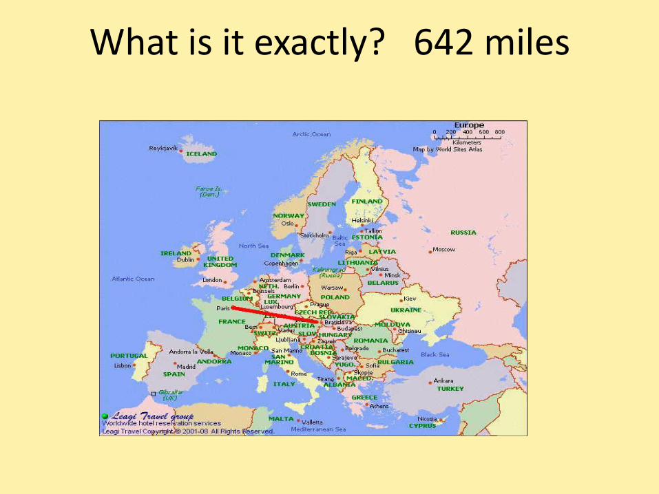
What is it exactly? 642 miles

Had enough?

• OK, I’m Done