teaching machines to understand data ... › ... › 2018-semantic-enrichment.pdfteaching machines...

TEACHING MACHINES TO UNDERSTAND DATA SCIENCE CODE BYSEMANTIC ENRICHMENT OF DATAFLOW GRAPHS

EVAN PATTERSON, IOANA BALDINI, ALEKSANDRA MOJSILOVIĆ, AND KUSH R. VARSHNEY

Abstract. Your computer is continuously executing programs, but does it really un-derstand them? Not in any meaningful sense. That burden falls upon human knowledgeworkers, who are increasingly asked to write and understand code. They deserve to haveintelligent tools that reveal the connections between code and its subject matter. Towardsthis prospect, we develop an AI system that forms semantic representations of computerprograms, using techniques from knowledge representation and program analysis. To cre-ate the representations, we introduce an algorithm for enriching dataflow graphs withsemantic information. The semantic enrichment algorithm is undergirded by a new on-tology language for modeling computer programs and a new ontology about data science,written in this language. Throughout the paper, we focus on code written by data scien-tists and we locate our work within a larger movement towards collaborative, open, andreproducible science.

1. Introduction

Your computer is continuously, efficiently, and reliably executing computer programs,but does it really understand them? Artificial intelligence researchers have taken greatstrides towards teaching machines to understand images, speech, natural text, and othermedia. The problem of understanding computer code has received far less attention overthe last two decades. Yet the growth of computing’s influence on society shows no signsof abating, with knowledge workers in all domains increasingly asked to create, maintain,and extend computer programs. For all workers, but especially those outside softwareengineering roles, programming is a means to achieve practical goals, not an end in itself.Programmers deserve intelligent tools that reveal the connections between their code, theircolleagues’ code, and the subject-matter concepts to which the code implicitly refers and towhich their real enthusiasm belongs. By teaching machines to comprehend code, we couldcreate artificial agents that empower human knowledge workers or perhaps even generateuseful programs of their own.

One computational domain undergoing particularly rapid growth is data science. Besidesthe usual problems facing the scientist-turned-programmer, the data scientist must contendwith a proliferation of programming languages (like Python, R, and Julia) and frameworks(too numerous to recount). Data science therefore presents an especially compelling targetfor machine understanding of computer code. An AI agent that simultaneously compre-hends the generic concepts of computing and the specialized concepts of data science couldprove enormously useful, by, for example, automatically visualizing machine learning work-flows or summarizing data analyses as natural text for human readers.

(Evan Patterson) Stanford Unversity, Statistics Department(Ioana Baldini, Aleksandra Mojsilović, Kush R. Varshney) IBM Research AIE-mail addresses: [email protected], [email protected], [email protected],

[email protected].

2 E. PATTERSON, I. BALDINI, A. MOJSILOVIĆ, AND K. R. VARSHNEY

Towards this prospect, we develop an AI system that forms semantic representations ofcomputer programs. Our system is fully automated, inasmuch as it expects nothing fromthe programmer besides the program itself and the ability to run it. We have designed oursystem to handle scripts written by data scientists, which tend to be shorter, more linear,and better defined semantically than the large-scale codebases written by software engineers.Our methodology is not universally applicable. Nevertheless, we think it could be fruitfullyextended to other scientific domains with a computational focus, such as bioinformatics orcomputational neuroscience, by integrating it with existing domain-specific ontologies.

We contribute several components that cohere as an AI system but also hold independentinterest. First, we define a dataflow graph representation of a computer program, calledthe raw flow graph. We extract raw flow graphs from computer programs using static anddynamic program analysis. We define another program representation, called the semanticflow graph, combining dataflow information with domain-specific information about datascience. To support the two representations, we introduce an ontology language for mod-eling computer programs, called Monocl, and an ontology written in this language, calledthe Data Science Ontology. Finally, we propose a semantic enrichment algorithm for trans-forming the raw flow graph into the semantic flow graph. The Data Science Ontology isavailable online1 and our system’s source code is available on GitHub under a permissiveopen source license (see Section 7).

Organization of paper. In the next section, we motivate our method through a pedagog-ical example (Section 2). We then explain the method itself, first informally and witha minimum of mathematics (Section 3) and then again with greater precision and rigor(Section 4). We divide the exposition in this way because the major ideas of the papercan be understood without the mathematical formalism, which may be unfamiliar to somereaders. We then take a step back from technical matters to locate our work within theongoing movement towards collaborative, open, and reproducible data science (Section 5).We also demonstrate our method on a realistic data analysis drawn from a biomedical datascience challenge. In the penultimate section, we bring out connections to existing work inartificial intelligence, program analysis, programming language theory, and category theory(Section 6). We conclude with directions for future research and development (Section 7).For a non-technical overview of our work, emphasizing motivation and examples, we suggestreading Sections 1, 2, 5 and 7.

2. First examples

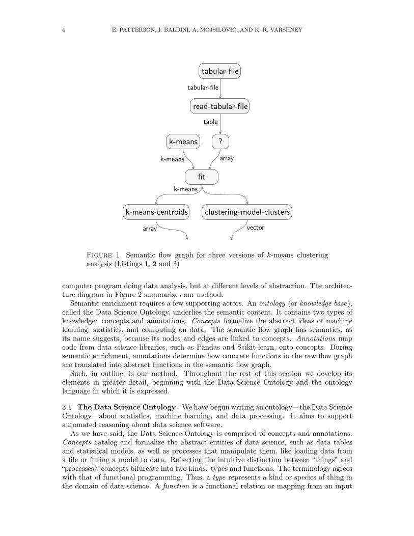
We begin with a small, pedagogical example, to be revisited and elaborated later. Threeversions of a toy data analysis are shown in Listings 1, 2 and 3. The first is written inPython using the scientific computing packages NumPy and SciPy; the second in Pythonusing the data science packages Pandas and Scikit-learn; and the third in R using the Rstandard library. The three programs perform the same analysis: they read the Iris datasetfrom a CSV file, drop the last column (labeling the flower species), fit a k-means clusteringmodel with three clusters to the remaining columns, and return the cluster assignmentsand centroids.

The programs are syntactically distinct but semantically equivalent. To be more precise,the programs are written in different programming languages—Python and R—and thetwo Python programs invoke different sets of libraries. Moreover, the programs exemplifydifferent programming paradigms. Listings 1 and 3 are written in functional style and

1To browse and search the Data Science Ontology, and to see additional documentation, please visithttps://www.datascienceontology.org.

https://www.datascienceontology.org

SEMANTIC ENRICHMENT OF DATAFLOW GRAPHS 3

import numpy as npfrom scipy.cluster.vq import kmeans2

iris = np.genfromtxt('iris.csv', dtype='f8', delimiter=',', skip_header=1)iris = np.delete(iris, 4, axis=1)

centroids, clusters = kmeans2(iris, 3)

Listing 1. k-means clustering in Python via NumPy and SciPy

import pandas as pdfrom sklearn.cluster import KMeans

iris = pd.read_csv('iris.csv')iris = iris.drop('Species', 1)

kmeans = KMeans(n_clusters=3)kmeans.fit(iris.values)centroids = kmeans.cluster_centers_clusters = kmeans.labels_

Listing 2. k-means cluster-ing in Python via Pandas andScikit-learn

iris = read.csv('iris.csv',stringsAsFactors=FALSE)

iris = iris[, names(iris) != 'Species']

km = kmeans(iris, 3)centroids = km$centersclusters = km$cluster

Listing 3. k-means clustering in R

Listing 2 is written in object-oriented style. Thus, at the syntactic level, the programsappear to be very different, and conventional program analysis tools would regard themas being very different. However, as readers fluent in Python and R will recognize, theprograms perform the same data analysis. They are semantically equivalent, up to possiblynumerical error and minor differences in the implementation of the k-means clusteringalgorithm. (Implementations differ mainly in how the iterative algorithm is initialized.)

Identifying the semantic equivalence, our system furnishes the same semantic flow graphfor all three programs, shown in Figure 1. The labeled nodes and edges refer to conceptsin the Data Science Ontology. The node tagged with a question mark refers to code withunknown semantics.

3. Ideas and techniques

We now explain our method of constructing semantic representations of computer pro-grams. At the highest level, two steps connect a computer program to its representations.First, computer program analysis distills the raw flow graph from the program. The rawflow graph is a dataflow graph that records the concrete function calls made during theexecution of the program. This graph is programming language and library dependent.In the second step, a process of semantic enrichment transforms the raw flow graph intothe semantic flow graph. The semantic flow graph describes the same program in termsof abstract concepts belonging to the Data Science Ontology. This graph is programminglanguage and library independent. Thus, both dataflow graphs capture the execution of a


clustering-model-clustersvector

?

fit

array

k-means

k-means

read-tabular-filetable

tabular-file

tabular-file

k-means-centroids

k-means

array

Figure 1. Semantic flow graph for three versions of k-means clusteringanalysis (Listings 1, 2 and 3)

computer program doing data analysis, but at different levels of abstraction. The architec-ture diagram in Figure 2 summarizes our method.

Semantic enrichment requires a few supporting actors. An ontology (or knowledge base),called the Data Science Ontology, underlies the semantic content. It contains two types ofknowledge: concepts and annotations. Concepts formalize the abstract ideas of machinelearning, statistics, and computing on data. The semantic flow graph has semantics, asits name suggests, because its nodes and edges are linked to concepts. Annotations mapcode from data science libraries, such as Pandas and Scikit-learn, onto concepts. Duringsemantic enrichment, annotations determine how concrete functions in the raw flow graphare translated into abstract functions in the semantic flow graph.

Such, in outline, is our method. Throughout the rest of this section we develop itselements in greater detail, beginning with the Data Science Ontology and the ontologylanguage in which it is expressed.

3.1. The Data Science Ontology. We have begun writing an ontology—the Data ScienceOntology—about statistics, machine learning, and data processing. It aims to supportautomated reasoning about data science software.

As we have said, the Data Science Ontology is comprised of concepts and annotations.Concepts catalog and formalize the abstract entities of data science, such as data tablesand statistical models, as well as processes that manipulate them, like loading data froma file or fitting a model to data. Reflecting the intuitive distinction between “things” and“processes,” concepts bifurcate into two kinds: types and functions. The terminology agreeswith that of functional programming. Thus, a type represents a kind or species of thing inthe domain of data science. A function is a functional relation or mapping from an input


Object values

Data science

ontology

Program executionProgram dataflow

analysis

Call stacks

Annotations

Language interpreter [Python, R, etc.]

Semantic

enrichment

User code & data

Raw flow graph

Semantic flow graph

Concepts &

annotations

Figure 2. System architecture

Table 1. Example concepts and annotations from the Data Science Ontology

Concept AnnotationType data table pandas data frame

statistical model scikit-learn estimator

Function reading a tabular data file read_csv function in pandas

fitting a statistical model todata

fit method of scikit-learn es-timators

type (the domain) to an output type (the codomain). In this terminology, the concepts ofa data table and of a statistical model are types, whereas the concept of fitting a predictivemodel is a function that maps an unfitted predictive model, together with predictors andresponse data, to a fitted predictive model.

As a modeling assumption, we suppose that software packages for data science, such asPandas and Scikit-learn, concretize the concepts. Annotations say how this concretizationoccurs by mapping types and functions in software packages onto type and function con-cepts in the ontology. To avoid confusion between levels of abstraction, we call the former“concrete” and the latter “abstract.” Thus, a type annotation maps a concrete type—a prim-itive type or user-defined class in a language like Python or R—onto an abstract type—atype concept. Likewise, a function annotation maps a concrete function onto an abstractfunction. We construe “concrete function” in the broadest possible sense to include anyprogramming language construct that “does something”: ordinary functions, methods ofclasses, attribute getters and setters, etc.

The division of the ontology into concepts and annotations on the one hand, and intotypes and functions on the other, leads to a two-way classification. Table 1 lists basicexamples of each of the four combinations, drawn from the Data Science Ontology.

Significant modeling flexibility is needed to accurately translate the diverse APIs ofstatistical software into a single set of universal concepts. Section 2 shows, for example, thatthe concept of k-means clustering can be concretized in software in many different ways.To accommodate this diversity, we allow function annotations to map a single concretefunction onto an arbitrary abstract “program” comprised of function concepts. In Figure 3,we display three function annotations relevant to the fitting of k-means clustering modelsin Listings 1, 2 and 3. By the end of this section, we will see how to interpret the three


k-means

integer

fit

array

k-means-centroidsarray

clustering-model-clustersvector

k-means

k-means

(a) Annotation: kmeans2 function in SciPy (cf. Listing 1)

fit

model data

model

(b) Annotation: fit method of BaseEstimatorclass in Scikit-learn (cf. Listing 2)

k-means

integer

fit

matrix

k-means

k-means

(c) Annotation: kmeans function in R’s builtinstats package (cf. Listing 3)

Figure 3. Example function annotations from the Data Science Ontology

annotations and how the semantic enrichment algorithm uses them to generate the semanticflow graph in Figure 1.

We have not yet said what kind of abstract “program” is allowed to appear in a func-tion annotation. Answering that question is the most important purpose of our ontologylanguage, to which we now turn.

3.2. The Monocl ontology language. The Data Science Ontology is expressed in anontology language that we call the MONoidal Ontology and Computing Language (Monocl).We find it helpful to think of Monocl as a minimalistic, typed, functional programminglanguage. The analogy usually suggests the right intuitions but is imperfect because Monoclis simpler than any commonly used programming language, being designed for knowledgerepresentation rather than actual computing.

The ontology language says how to construct new types and functions from old, for thepurposes of defining concepts and annotations. Monocl is written in a point-free textualsyntax or equivalently in a graphical syntax of interconnected boxes and wires. The twosyntaxes are parallel though not quite isomorphic. In this section, we emphasize the more


intuitive graphical syntax. We describe the constructors for types and functions and illus-trate them using the graphical syntax. A more formal development is given in Section 4.2.

Monocl has a minimalistic type system, supporting product and unit types as well asa simple form of subtyping. A basic type, sometimes called a “primitive type,” is a typethat cannot be decomposed into simpler types. Basic types must be explicitly defined. Allother types are composite. For instance, the product of two types X and Y is another typeX × Y . It has the usual meaning: an element of type X × Y is an element of type X andan element of type Y , in that order. Products of three or more types are defined similarly.Product types are similar to record types in conventional programming languages, such asstruct types in C. There is also a unit type 1 inhabited by a single element. It is analogousto the void type in C and Java, the NoneType type in Python (whose sole inhabitant isNone), and the NULL type in R.

A type can be declared a subtype of one or more other types. To a first approximation,subtyping establishes an “is-a” relationship between types. In the Data Science Ontology,matrices are a subtype of both arrays (being arrays of rank 2) and data tables (being ta-bles whose columns all have the same data type). As this example illustrates, subtypingin Monocl differs from inheritance in a typical object-oriented programming language. In-stead, subtyping should be understood through implicit conversion, also known as coercion(Reynolds 1980; Pierce 1991). The idea is that if a type X is a subtype of X ′, then thereis a canonical way to convert elements of type X into elements of type X ′. Elaboratingour example, a matrix simply is an array (of rank 2), hence can be trivially converted intoan array. A matrix is not strictly speaking a data table but can be converted into one (ofhomogeneous data type) by assigning numerical names to the columns.

In the graphical syntax, types are represented by wires. A basic type X is drawn as asingle wire labeled X. A product of n types is a bundle of n wires in parallel. The unittype is an empty bundle of wires (a blank space). This should become clearer as we discusswiring diagrams for functions.

A function f in Monocl has an input type X, its domain, and an output type Y , itscodomain. We express this in the usual mathematical notation as f : X → Y . Like types,functions are either basic or composite. Note that a basic function may have compositedomain or codomain. From the programming languages perspective, a program in theMonocl language is nothing more than a function.

Functions are represented graphically by wiring diagrams (also known as string dia-grams). A basic function f : X → Y is drawn as a box labeled f . The top of the box hasinput ports with incoming wires X and the bottom has output ports with outgoing wiresY . A wiring diagram defines a general composite function by connecting boxes with wiresaccording to certain rules. The diagram has an outer box with input ports, defining thefunction’s domain, and output ports, defining the codomain. Figures 1, 3, 5, 6, 7 and 8 areall examples of wiring diagrams.

The rules for connecting boxes within a wiring diagram correspond to ways of creatingnew functions from old. The two most fundamental ways are composing functions andtaking products of functions. The composition of a function f : X → Y with g : Y → Zis a new function f · g : X → Z, with the usual meaning. Algorithmically speaking, f · gcomputes in sequence: first f and then g. The product of functions f : X → W andg : Y → Z is another function f × g : X × Y →W ×Z. Algorithmically, f × g computes fand g in parallel, taking the inputs, and returning the outputs, of both f and g. Figures 4aand 4b show the graphical syntax for composition and products.

The graphical syntax implicitly includes a number of special functions. For any type X,the identity function 1X : X → X maps every element of type X to itself. For each pair of


f

X

g

Y

Z

(a) Composition

f

X

g

Y

W Z

(b) Product

f

X

Y Y

(c) Copying data

f

X

(d) Deleting data

Figure 4. Graphical syntax for operations on functions

types X and Y , the braiding or transposition function σX,Y : X × Y → Y ×X exchangesits two inputs. Identities and braidings are drawn as straight wires and pairs of crossedwires, respectively. Any permutation function can be expressed by taking compositionsand products of identities and braidings. Diagrammatically, this means that a bundle ofwires may be criss-crossed in arbitrarily complex ways (provided that the wires do not bendbackwards). For each type X, there is also a copying function ∆X : X → X × X, whichduplicates its input, and a deleting function ♦X : X → I, which discards its input. Inthe graphical syntax, these functions allow a single output port to have multiple or zerooutgoing wires. For instance, given a function f : X → Y , Figures 4c and 4d display thecompositions f · ∆Y : X → Y × Y and f · ♦Y : X → I. The analogous situation is notpermitted of input ports; in a well-formed wiring diagram, every input port has exactly oneincoming wire.

Besides serving as the “is-a” relation ubiquitous in knowledge representation systems,the subtype relation for objects enables ad hoc polymorphism for functions. We extendthe definition of function composition to include implicit conversion, namely, to compose afunction f : X → Y with g : Y ′ → Z, we require not necessarily that Y equals Y ′, but onlythat Y be a subtype of Y ′. Operationally, to compute f · g, we first compute f , then coercethe result from type Y to Y ′, and finally compute g. Diagrammatically, a wire connectingtwo boxes has valid types if and only if the source port’s type is a subtype of the targetport’s type. Thus implicit conversions really are implicit in the graphical syntax.

Monocl also supports “is-a” relations between functions, which we call subfunctions inanalogy to subtypes. In the Data Science Ontology, reading a table from a tabular file (callit f) is a subfunction of reading data from a generic data source (call it f ′). That soundsintuitively plausible but what does it mean? The domain of f , a tabular file, is a subtypeof the domain of f ′, a generic data source. The codomain of f , a table, is a subtype of thecodomain of f ′, generic data. Now consider two possible computational paths that take atabular file and return generic data. We could apply f , then coerce the resulting table togeneric data. Alternatively, we could coerce the tabular file to a generic data source, thenapply f ′. The subfunction relation asserts that these two computations are equivalent. Thegeneral definition of a subfunction is perfectly analogous.

3.3. Raw and semantic dataflow graphs. With this preparation, we can attain a moreexact understanding of the raw and semantic flow graphs. The two dataflow graphs areboth wiring diagrams representing a data analysis. However, they exist at different levelsof abstraction.


The raw flow graph describes the computer implementation of a data analysis. Its boxesare concrete functions or, more precisely, the function calls observed during the executionof the program. Its wires are concrete types together with their observed elements. These“elements” are either literal values or object references, depending on the type. To illustrate,Figures 5, 6 and 7 show the raw flow graphs for Listings 1, 2 and 3, respectively. Note thatthe wire elements are not shown.

The semantic flow graph describes a data analysis in terms of universal concepts, in-dependent of the particular programming language and libraries used to implement theanalysis. Its boxes are function concepts. Its wires are type concepts together with theirobserved elements. The semantic flow graph is thus an abstract function, composed of theontology’s concepts and written in the graphical syntax, but augmented with computedvalues. Figure 1 shows the semantic flow graph for Listings 1, 2 and 3. Another semanticflow graph is shown in Figure 8 below. Again, the wire elements are not shown.

3.4. Program analysis. We use computer program analysis to extract the raw flow graphfrom a data analysis. Program analysis therefore plays an essential role in our AI system.It plays an equally important role in our original publication on this topic (Patterson,McBurney, et al. 2017), reviewed below in Section 6. In the present work, we have extendedour program analysis tools to support the R language, but our basic methodology haschanged little. We review only the major points about our usage of computer programanalysis, deferring to our original paper for details.

Program analysis can be static or dynamic or both. Static analysis consumes the sourcecode but does not execute it. Much literature on program analysis is about static analysisbecause of its relevance to optimizing compilers (F. Nielson, H. R. Nielson, and Hankin 1999;Aho et al. 2006). Dynamic analysis, in contrast, executes the program without necessarilyinspecting the code.

Our program analysis is mainly dynamic, for a couple of reasons. Static analysis, espe-cially type inference, is challenging for the highly dynamic languages popular among datascientists. Moreover, we record values computed over the course of the program’s execution,such as model parameters and hyperparameters. For this dynamic analysis is indispens-able. Of course, a disadvantage of dynamic analysis is the necessity of running the program.Crucially, our system needs not just the code itself, but its input data and runtime environ-ment. These are all requirements of scientific reproducibility (see Section 5), so in principlethey ought to be satisfied. In practice they are often neglected.

To build the raw flow graph, our program analysis tools record interprocedural dataflow during program execution. We begin with the empty wiring diagram and add boxesincrementally as the program unfolds. Besides recording function calls and their argumentsand return values, the main challenge is to track the provenance of objects as they arepassed between functions. When a new box is added to the diagram, the provenance recordsays how to connect the input ports of the new box to the output ports of existing boxes.

How all this is accomplished depends on the programming language in question. InPython, we register callbacks via sys.settrace, to be invoked whenever a function iscalled or returns. A table of object provenance is maintained using weak references. Nomodification of the abstract syntax tree (AST) is necessary. In R, we add callbacks byrewriting the AST, to be invoked whenever a term is (lazily) evaluated. Care must betaken to avoid breaking functions which use nonstandard evaluation, a kind of dynamicmetaprogramming unique to R (Wickham 2014).

Our usage of program analysis involves conceptual as well as engineering difficulties,because the programming model of Monocl is simpler than that of typical programming


genfromtxt

delete

ndarray

kmeans2

ndarray

ndarray ndarray

Figure 5. Raw flow graph for k-means clustering in Python via NumPyand SciPy (Listing 1)

_make_parser_function.<locals>.parser_f

DataFrame.drop

DataFrame

values

DataFrame

KMeans

KMeans.fit

KMeans ndarray

cluster_centers_

KMeans

labels_

ndarray ndarray

Figure 6. Raw flow graphfor k-means clustering inPython via Pandas andScikit-learn (Listing 2)

centers

kmeans

kmeans

cluster

read.csv

names

data.frame

[

!=

character

logical

data.frame

Figure 7. Raw flow graphfor k-means clustering in R(Listing 3)


languages. We mention just one conceptual problem to give a sense of the issues that arise.Monocl is purely functional, whereas most practical languages allow mutation of objects.2Our program analysis tools have limited capabilities for detecting mutations. When a“function” mutates an object, the mutated object is represented in the raw flow graph as anextra output of the function. For instance, we interpret the fit method of a Scikit-learnestimator, which modifies the model in-place, as returning a new model (Figure 3b).

3.5. Semantic enrichment. The semantic enrichment algorithm transforms the raw flowgraph into the semantic flow graph. It proceeds in two independent stages, one of expan-sion and one of contraction. The expansion stage makes essential use of the ontology’sannotations.

Expansion. In the expansion stage, the annotated parts of the raw flow graph are replacedby their abstract definitions. Each annotated box—that is, each box referring to a concretefunction annotated by the ontology—is replaced by the corresponding abstract function.Likewise, the concrete type of each annotated wire is replaced by the corresponding abstracttype. This stage of the algorithm is “expansionary” because, as we have seen, a functionannotation’s definition may be an arbitrary Monocl program. In other words, a single boxin the raw flow graph may expand to an arbitrarily large subdiagram in the semantic flowgraph.

The expansion procedure is functorial, to use the jargon of category theory. Informally,this means two things. First, notice that concrete types are effectively annotated twice,explicitly by type annotations and implicitly by the domain and codomain types in functionannotations. Functorality requires that these abstract types be compatible, ensuring thelogical consistency of type and function annotations. Second, expansion preserves thestructure of the ontology language, including composition and products. Put differently,the expansion of a wiring diagram is completely determined by its action on individual boxes(basic functions). Functorality is a modeling decision that greatly simplifies the semanticenrichment algorithm, at the expense of imposing restrictions on how the raw flow graphmay be transformed.

Contraction. It is practically infeasible to annotate every reusable unit of data sciencesource code. Most real-world data analyses use concrete types and functions that are notannotated. This unannotated code has unknown semantics, so properly speaking it doesnot belong in the semantic flow graph. On the other hand, it usually cannot be deletedwithout altering the dataflow in the rest of the diagram. Semantic enrichment must notcorrupt the dataflow record.

As a compromise, in the contraction stage, the unannotated parts of the raw flow graphare simplified to the extent possible. All references to unannotated types and functions areremoved, leaving behind unlabeled wires and boxes. Semantically, the unlabeled wires areinterpreted as arbitrary “unknown” types and the unlabeled boxes as arbitrary “unknown”functions (which could have known domain and codomain types). The diagram is thensimplified by encapsulating unlabeled boxes. Specifically, every maximal connected subdi-agram of unlabeled boxes is encapsulated by a single unlabeled box. The interpretation isthat any composition of unknown functions is just another unknown function. This stageis “contractionary” because it can only decrease the number of boxes in the diagram.

2Mutation is more common in Python than in R because most R objects have copy-on-modify semantics.


Example revisited. To reprise our original example, semantic enrichment transforms the rawflow graphs of Figures 5, 6 and 7 into the same semantic flow graph, shown in Figure 1.Let us take a closer look at a few of the expansions and contractions involved.

Expansions related to k-means clustering occur in all three programs. In the Pythonprogram based on SciPy (Figure 5), the kmeans2 function expands into a program thatcreates a k-means clustering model, fits it to the data, and extracts its cluster assignmentsand centroids, as described by the annotation in Figure 3a. The abstract k-means clusteringmodel does not correspond to any concrete object in the original program. We routinelyuse this modeling pattern to cope with functions that are not object-oriented with respectto models.

By contrast, the Python program based on Scikit-learn (Figure 6) is written in object-oriented style. The KMeans class expands to an abstract k-means clustering type. The fitmethod of the KMeans class is not annotated in the Data Science Ontology. However, thefit method of the superclass BaseEstimator is annotated (Figure 3b), so the expansionis performed using that annotation. As this case illustrates, subtyping and polymorphismare indispensable when annotating object-oriented code.

The R program (Figure 7) is intermediate between these two styles. The kmeans function,annotated in Figure 3c, directly takes the data and the number of clusters, but returns anobject of class kmeans. The cluster assignments and centroids are slots of this object,annotated separately. This design pattern is typical in R, due to its informal type system.

Now consider the contractions. In the first program (Figure 5), the only unannotatedbox is NumPy’s delete function. Contracting this box does not reduce the size of thewiring diagram. A contraction involving multiple boxes occurs in the second program(Figure 6). The subdiagram consisting of the pandas NDFrame.drop method composedwith the values attribute accessor is encapsulated into a single unlabeled box. We haveleft these functions unannotated for the sake of illustration and because the section of theData Science Ontology dedicated to data manipulation has not yet been developed. Weexpect this gap to close as the ontology grows.

4. Mathematical foundations

To put the foregoing ideas on a firmer footing, we formalize the ontology and the semanticenrichment algorithm in the language of category theory. We are not professional categorytheorists and we have tried to make this section accessible to other non-category theorists.Nevertheless, readers will find it helpful to have a working knowledge of basic categorytheory, as may be found in the introductory textbooks (Spivak 2014; Awodey 2010; Leinster2014; Riehl 2016), and of monoidal category theory, as in the survey articles (Baez and Stay2010; Coecke and Paquette 2010). For readers without this background, or who simply wishto understand our method informally, this section can be skipped without loss of continuity.

Here, in outline, is our program. We take the ontology’s concepts to form a category, withtype concepts corresponding to objects and function concepts corresponding to morphisms.Defining the ontology language amounts to fixing a categorical doctrine, which will turnout to be the doctrine of cartesian categories with implicit conversion. Up to this point, weconform to the general scheme of categorical knowledge representation, according to whichontologies are simply categories in a suitable doctrine (Spivak and Kent 2012; Patterson2017). Having defined the ontology’s concepts as a category C, we then interpret theannotations as a partial functor from a category L modeling a software ecosystem to theconcept category C. Finally, we formalize the raw and semantic flow graphs as morphismsin categories of elements over L and C.


4.1. Why category theory? Because category theory does not yet belong to the basictoolbox of knowledge representation, we pause to motivate the categorical approach beforelaunching into the formal development. Why is category theory an appealing frameworkfor representing knowledge, especially about computational processes? We offer severalanswers to this question.

First, there already exist whole branches of computer science, namely type theory andprogramming language theory, dedicated to the mathematical modeling of computer pro-grams. To neglect them in knowledge representation would be unfortunate. Categorytheory serves as an algebraic bridge to these fields. Due to the close connection betweencategory theory and type theory (Crole 1993; Jacobs 1999)—most famously, the correspon-dence between cartesian closed categories and simply typed lambda theories (Lambek andScott 1988)—we may dwell in the syntactically and semantically flexible world of algebrabut still draw on the highly developed theory of programming languages. In Section 4.2, weborrow specific notions of subtyping and ad hoc polymorphism from programming languagetheory (Goguen 1978; Reynolds 1980).

Category theory is also useful in its own right, beyond its connection to programminglanguage theory. The essential innovation of category theory over the mainly syntacticaltheory of programming languages is that programs become algebraic structures, analogousto, albeit more complicated than, classical algebraic structures like groups and monoids.Like any algebraic structure, categories of programs are automatically endowed with anappropriate notion of structure-preserving map between them. In this case, the structure-preserving maps are a special kind of functor. In Section 4.3, we formulate the semanticenrichment algorithm as a functor between categories of programs. The structuralist phi-losophy underlying modern algebra is therefore central to our whole approach.

Another advantage of category theory is flexibility of syntax. Unlike the lambda calculusand other type theories, algebraic structures like categories exist independently of anyparticular system of syntax. Syntactic flexibility is mathematically convenient but alsopractically important. Monoidal categories admit a graphical syntax of wiring diagrams,also known as string diagrams (Baez and Stay 2010; Selinger 2010). We introduced thegraphical syntax informally in Section 3.2. It offers an intuitive yet rigorous alternativeto the typed lambda calculus’s textual syntax (Selinger 2013), which beginners may findimpenetrable. The family of graphical languages based on string diagrams is a jewel ofcategory theory, with applications to such diverse fields as quantum mechanics (Coeckeand Paquette 2010), control theory (Baez and Erbele 2015), and natural language semantics(Coecke, Grefenstette, and Sadrzadeh 2013).

Having arrived at the general categorical perspective, the next question to ask is: whatkind of category shall we use to model computer programs? We begin our investigationwith cartesian categories, which are perhaps the simplest possible model of typed, functionalcomputing. As we recall more carefully in Section 4.2, cartesian categories are symmetricmonoidal categories with natural operations for copying and deleting data. Morphisms ina cartesian category behave like mathematical functions.

As a model of computation, cartesian categories are very primitive. They do not allow formanipulating functions as data (via lambda abstraction) or for recursion (looping), hencethey can only express terminating computations of fixed, finite length. Extensions of thiscomputational model abound. Cartesian closed categories arise as cartesian categories witha closed structure, whereby the whole collection of morphisms X → Y is representable asan exponential object Y X . Closed categories have function types, in programming jargon.According to a famous result, cartesian closed categories are equivalent to the typed lambdacalculus (Lambek and Scott 1988). Traced symmetric monoidal categories model looping


and other forms of feedback. According to another classic result, a trace on a cartesiancategory is equivalent to a Conway fixed point operator (Hasegawa 1997; Hasegawa 2003).Fixed points are used in programming language theory to define the semantics of recursion.Combining these threads, we find in traced cartesian closed categories a Turing-completemodel of functional computing, amounting to the typed lambda calculus with a fixed pointoperator.

Relaxing the cartesian or even the monoidal structure is another way to boost modelingflexibility. Starting with the cartesian structure, we interpret morphisms that are unnaturalwith respect to copying as performing non-deterministic computation, such as randomnumber generation or Monte Carlo sampling. We interpret morphisms unnatural withrespect to deleting as partial functions, because they raise errors or are undefined on certaininputs. In a symmetric monoidal category C with diagonals (not necessarily cartesian), themorphisms that do satisfy the naturality conditions for copying and deleting data forma cartesian subcategory of C, called the cartesian center or focus of C (Selinger 1999).It is also possible to relax the monoidal product itself. Symmetric premonoidal categoriesmodel side effects and imperative programs, where evaluation order matters even for parallelstatements, such as variable access and assignment. Any premonoidal category has a centerthat is a monoidal category (Power and Robinson 1997). Thus, classical computationalprocesses form a three-level hierarchy: a symmetric premonoidal category has a center thatis symmetric monoidal, which in turn has a cartesian center (Jeffrey 1997).

This short survey hardly exhausts the categorical structures that have been used to modelcomputer programs. However, our purpose here is not to define the most general modelpossible, but rather to adopt the simplest model that still captures useful information inpractice. For us, that model is the cartesian category. The structures in this categoricaldoctrine agree with the features currently supported by our program analysis tools (Sec-tion 3.4). We expect that over time our software will acquire more features and achievebetter fidelity, whereupon we will adopt a more expressive doctrine. The survey aboveshows that this transition can happen smoothly. In general, modularity is a key advantageof categorical knowledge representation: category theory provides a toolkit of mathematicalstructures that can be assembled in more or less complex ways to meet different modelingneeds.

Notation. We compose our maps in diagrammatic (left-to-right) order. In particular, wewrite the composition of a morphism f : X → Y with another morphism g : Y → Z asf · g : X → Z or simply fg : X → Z. Small categories C,D,E, . . . are written in script fontand large categories in bold font. As standard examples of the latter, we write Set for thecategory of sets and functions and Cat for the category of (small) categories and functors.Other categories will be introduced as needed.

4.2. Concepts as category. We formalize the ontology as a category. The type and func-tion concepts in the ontology are, respectively, the objects and morphisms that generatethe category. Abstract programs expressed in terms of concepts correspond to general mor-phisms in the category, assembled from the object and morphism generators by operationslike composition and monoidal products. In this subsection, we develop the categoricaldoctrine where the ontology category will reside, by augmenting cartesian categories, moti-vated in Section 4.1, with a form of subtyping based on implicit conversion. Ultimately, wedefine a Monocl ontology to be a finite presentation of a cartesian category with implicitconversion.


The definition of diagonals in a monoidal category is fundamental (Selinger 1999). Instating it, we take for granted the definition of a symmetric monoidal category ; see thereferences at the beginning of this section for further reading.

Definition. A monoidal category with diagonals is a symmetric monoidal category (C,×, 1)together with two families of morphisms,

∆X : X → X ×X and ♦X : X → 1,

indexed by objects X ∈ C. The morphisms ∆X and ♦X , called copying and deleting,respectively, are required to make X into a cocommutative comonoid (the formal dual of acommutative monoid). Moreover, the families must be coherent, or uniform, in the sensethat ♦1 = 11 and for all objects X,Y ∈ C, the diagrams commute:

X × Y X ×X × Y × Y

X × Y ×X × Y

∆X×∆Y

∆X×Y

1X×σX,Y ×1Y

X × Y 1× 1

1

♦X×♦Y

♦X×Y

∼=

As explained in graphical terms in Section 3.2, the copying and deleting morphismsallow data to be duplicated and discarded, a basic feature of classical (but not quantum)computation. Uniformity is a technical condition ensuring that copying and deleting arecompatible with the symmetric monoidal structure. So, for example, a uniform copyingoperation has the property that copying data of type X×Y is equivalent to simultaneouslycopying data of type X and copying data of type Y , up to the ordering of the outputs.

A monoidal category with diagonals is a very general algebraic structure. Its morphismsneed not resemble computational processes in any conventional sense. However, adding justone additional axiom yields the cartesian category, a classical notion in category theory anda primitive model of functional computing.

Definition. A cartesian category is a monoidal category with diagonals whose copying anddeleting maps, ∆X and ♦X , are natural in X, meaning that for any morphism f : X → Y ,the diagrams commute:

X Y

X ×X Y × Y

f

∆X ∆Y

f×f

X Y

1

f

♦X♦Y

We denote by Cart the category of (small) cartesian categories and cartesian functors(strong monoidal functors preserving the diagonals).

Remark. Although it is not obvious, this definition of cartesian category is equivalent tothe standard definition via the universal property of finite products (Heunen and Vicary2012). We prefer the alternative definition given here because it is phrased in the languageof monoidal categories and string diagrams.

In a cartesian category, the naturality conditions on copying and deleting assert thatcomputation is deterministic and total. In more detail, naturality of copying says thatcomputing a function f , then copying the output is the same as copying the input, thencomputing f on both copies. This means that f always produces the same output on agiven input, i.e., f is deterministic. Naturality of deleting says that computing the functionf , then deleting the output is the same as simply deleting the input. This means that f is


well-defined on all its inputs, i.e., f is total. Together, the naturality conditions establishthat the category’s morphisms behave like mathematical functions.

Cartesian categories are perhaps the simplest model of typed, functional computing, aswe argued in Section 4.1. We considered there several extensions and relaxations of thecartesian structure, all centered around morphisms. One can also entertain richer construc-tions on objects. In programming jargon, this amounts to adding a more elaborate typesystem. A cartesian category has a type system with product and unit types, introducedfrom the programming languages perspective in Section 3.2.

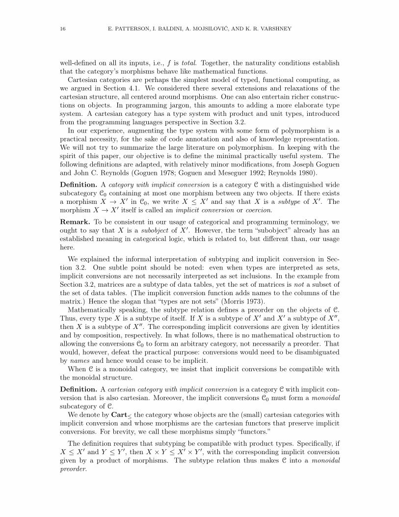
In our experience, augmenting the type system with some form of polymorphism is apractical necessity, for the sake of code annotation and also of knowledge representation.We will not try to summarize the large literature on polymorphism. In keeping with thespirit of this paper, our objective is to define the minimal practically useful system. Thefollowing definitions are adapted, with relatively minor modifications, from Joseph Goguenand John C. Reynolds (Goguen 1978; Goguen and Meseguer 1992; Reynolds 1980).

Definition. A category with implicit conversion is a category C with a distinguished widesubcategory C0 containing at most one morphism between any two objects. If there existsa morphism X → X ′ in C0, we write X ≤ X ′ and say that X is a subtype of X ′. Themorphism X → X ′ itself is called an implicit conversion or coercion.

Remark. To be consistent in our usage of categorical and programming terminology, weought to say that X is a subobject of X ′. However, the term “subobject” already has anestablished meaning in categorical logic, which is related to, but different than, our usagehere.

We explained the informal interpretation of subtyping and implicit conversion in Sec-tion 3.2. One subtle point should be noted: even when types are interpreted as sets,implicit conversions are not necessarily interpreted as set inclusions. In the example fromSection 3.2, matrices are a subtype of data tables, yet the set of matrices is not a subset ofthe set of data tables. (The implicit conversion function adds names to the columns of thematrix.) Hence the slogan that “types are not sets” (Morris 1973).

Mathematically speaking, the subtype relation defines a preorder on the objects of C.Thus, every type X is a subtype of itself. If X is a subtype of X ′ and X ′ a subtype of X ′′,then X is a subtype of X ′′. The corresponding implicit conversions are given by identitiesand by composition, respectively. In what follows, there is no mathematical obstruction toallowing the conversions C0 to form an arbitrary category, not necessarily a preorder. Thatwould, however, defeat the practical purpose: conversions would need to be disambiguatedby names and hence would cease to be implicit.

When C is a monoidal category, we insist that implicit conversions be compatible withthe monoidal structure.

Definition. A cartesian category with implicit conversion is a category C with implicit con-version that is also cartesian. Moreover, the implicit conversions C0 must form a monoidalsubcategory of C.

We denote by Cart≤ the category whose objects are the (small) cartesian categories withimplicit conversion and whose morphisms are the cartesian functors that preserve implicitconversions. For brevity, we call these morphisms simply “functors.”

The definition requires that subtyping be compatible with product types. Specifically, ifX ≤ X ′ and Y ≤ Y ′, then X × Y ≤ X ′ × Y ′, with the corresponding implicit conversiongiven by a product of morphisms. The subtype relation thus makes C into a monoidalpreorder.


Remark. Asking C0 to inherit the cartesian or even the symmetric monoidal structure leadsto undesirable consequences, such as unwanted implicit conversions and even strictificationof the original category C. Namely, if C0 is a symmetric monoidal subcategory of C, thenthe braidings σX,Y : X × Y → Y ×X in C must satisfy σX,X = 1X×X , which is false underthe intended set-theoretic interpretation.

Because our notion of subtyping is operationalized by the implicit conversions, we canextend it from objects to morphisms through naturality squares.

Definition. Let C be a category with implicit conversion. A morphism f in C is a submor-phism (or subfunction) of another morphism f ′, written f ≤ f ′, if in the arrow categoryC→ there exists a (unique) morphism f → f ′ whose components are implicit conversions.

Explicitly, if f : X → Y and f ′ : X ′ → Y ′ are morphisms in C, with X ≤ X ′ and Y ≤ Y ′,then f ≤ f ′ if and only if the diagram commutes:

X Y

X ′ Y ′

f

≤ ≤f ′

Remark. In a closed category, subtypes of basic types, X ≤ X ′ and Y ≤ Y ′, canonicallyinduce subtypes of function types, Y X′ ≤ (Y ′)X , by “restricting the domain” and “expandingthe codomain.” Be warned that this construction is not the same as a submorphism (it iscontravariant in X, while a submorphism is covariant in both X and Y ). Indeed, we donot treat cartesian closed categories at all in this paper.

Again, see Section 3.2 for informal interpretation and examples of this notion. Just assubtypes define a preorder on the objects of C, submorphisms define a preorder on themorphisms of C. Moreover, submorphisms respect the compositional structure of C. Theyare closed under identities, i.e., 1X ≤ 1X′ whenever X ≤ X ′, and under composition, i.e., iff ≤ f ′ and g ≤ g′ are composable, then fg ≤ f ′g′. All these statements are easy to prove.To illustrate, transitivity and closure under composition are proved by pasting commutativesquares vertically and horizontally:

X Y

X ′ Y ′

X ′′ Y ′′

f

≤ ≤f ′

≤ ≤f ′′

X Y Z

X ′ Y ′ Z ′

f

≤

g

≤ ≤f ′ g′

When C is a cartesian category with implicit conversion, submorphisms are also closedunder products: if f ≤ f ′ and g ≤ g′, then f × g ≤ f ′ × g′, because, by functorality,monoidal products preserve commutative diagrams.

We now define an ontology to be nothing other than a finitely presented cartesian categorywith implicit conversion. More precisely:

Definition. An ontology in the Monocl language is a cartesian category with implicit con-version, given by a finite presentation. That is, it is the cartesian category with implicitconversion generated by finite sets of:

• basic types, or object generators, X• basic functions, or morphism generators, f : X → Y , where X and Y are objects


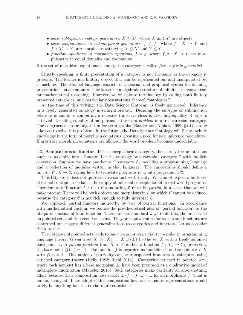
• basic subtypes, or subtype generators, X ≤ X ′, where X and X ′ are objects• basic subfunctions, or submorphism generators, f ≤ f ′, where f : X → Y andf ′ : X ′ → Y ′ are morphisms satisfying X ≤ X ′ and Y ≤ Y ′• function equations, or morphism equations, f = g, where f, g : X → Y are mor-phisms with equal domains and codomains.

If the set of morphism equations is empty, the category is called free or freely generated.

Strictly speaking, a finite presentation of a category is not the same as the category itpresents. The former is a finitary object that can be represented on, and manipulated by,a machine. The Monocl language consists of a textual and graphical syntax for definingpresentations on a computer. The latter is an algebraic structure of infinite size, convenientfor mathematical reasoning. However, we will abuse terminology by calling both finitelypresented categories, and particular presentations thereof, “ontologies.”

At the time of this writing, the Data Science Ontology is freely generated. Inferencein a freely generated ontology is straightforward. Deciding the subtype or subfunctionrelations amounts to computing a reflexive transitive closure. Deciding equality of objectsis trivial. Deciding equality of morphisms is the word problem in a free cartesian category.The congruence closure algorithm for term graphs (Baader and Nipkow 1999, §4.4) can beadapted to solve this problem. In the future, the Data Science Ontology will likely includeknowledge in the form of morphism equations, creating a need for new inference procedures.If arbitrary morphism equations are allowed, the word problem becomes undecidable.

4.3. Annotations as functor. If the concepts form a category, then surely the annotationsought to assemble into a functor. Let the ontology be a cartesian category C with implicitconversion. Suppose we have another such category L, modeling a programming languageand a collection of modules written in that language. The annotations should define afunctor F : L→ C, saying how to translate programs in L into programs in C.

This tidy story does not quite survive contact with reality. We cannot expect a finite setof formal concepts to exhaust the supply of informal concepts found in real-world programs.Therefore any “functor” F : L → C annotating L must be partial, in a sense that we willmake precise. There will be both objects and morphisms in L on which F cannot be defined,because the category C is not rich enough to fully interpret L.

We approach partial functors indirectly, by way of partial functions. In accordancewith mathematical custom, we reduce the pre-theoretical idea of “partial function” to theubiquitous notion of total function. There are two standard ways to do this, the first basedon pointed sets and the second on spans. They are equivalent as far as sets and functions areconcerned but suggest different generalizations to categories and functors. Let us considerthem in turn.

The category of pointed sets leads to one viewpoint on partiality, popular in programminglanguage theory. Given a set X, let X⊥ := X t {⊥} be the set X with a freely adjoinedbase point ⊥. A partial function from X to Y is then a function f : X⊥ → Y⊥ preservingthe base point (f(⊥) = ⊥). The function f is regarded as “undefined” on the points x ∈ Xwith f(x) = ⊥. This notion of partiality can be transported from sets to categories usingenriched category theory (Kelly 1982; Riehl 2014). Categories enriched in pointed sets,where each hom-set has a base morphism ⊥, have been proposed as a qualitative model ofincomplete information (Marsden 2016). Such categories make partiality an all-or-nothingaffair, because their composition laws satisfy ⊥·f = f ·⊥ = ⊥ for all morphisms f . That isfar too stringent. If we adopted this composition law, our semantic representations wouldrarely be anything but the trivial representation ⊥.


Alternatively, a partial function can be defined as a special kind of span of total functions.Now let us say that a partial function from X to Y is a span in Set

I

X Y

ι f

whose left leg ι : I → X is monic (injective). The partial function’s domain of definitionis I, which we regard as a subset of X. Although we shall not need it here, we note thatpartial functions, and partial morphisms in general, can be composed by taking pullbacks(Borceux 1994, §5.5).

We interpret the span above as partially defining a function f on X, via a set of equationsindexed by I:

f(xi) := yi, i ∈ I.

It is then natural to ask: what is the most general way to define a total function on Xobeying these equations? The answer is given by the pushout in Set:

I

X Y

Y∗

ι f

pf∗ ι∗

Because ι : I → X is monic, so is ι∗ : Y → Y∗, and we regard Y as a subset of Y∗. Thecommutativity of the diagram says that f∗ satisfies the set of equations indexed by I. Theuniversal property defining the pushout says that any other function f ′ : X → Y ′ satisfyingthe equations factors uniquely through f∗, meaning that there exists a unique functiong : Y∗ → Y ′ making the diagram commute:

I

X Y∗ Y

Y ′

ι f

f∗

f ′g

ι∗

ι′

The codomain of the function f∗ : X → Y∗ consists of Y plus a “formal image” f(x) foreach element x on which f is undefined. Contrast this with the codomain of a functionX → Y⊥, which consists of Y plus a single element ⊥ representing all the undefined values.

This viewpoint on partiality generalizes effortlessly from Set to any category with pushouts.We partially define the annotations as a span in Cart≤

I

L C

ι F


whose left leg ι : I→ L is monic. We then form the pushout in Cart≤:

I

L C

C∗

ι F

pF∗ ι∗

Given a morphism f in L, which represents a concrete program, its image F∗(f) in C∗ is apartial translation of the program into the language defined by the ontology’s concepts.

The universal property of the pushout in Cart≤, stated above in the case of Set, givesan appealing intuitive interpretation to program translation. The category C is not richenough to fully translate L via a functor L → C. As a modeling assumption, we supposethat C has some “completion” C for which a full translation F : L → C is possible. Wedo not know C, or at the very least we cannot feasibly write it down. However, if we takethe pushout functor F∗ : L → C∗, we can at least guarantee that, no matter what thecomplete translation F is, it will factor through F∗. Thus F∗ defines the most generalpossible translation, given the available information.

The properties of partial functions largely carry over to partial functors, with one im-portant exception: the “inclusion” functor ι∗ : C → C∗ need not be monic, even thoughι : I → L is. Closely related is the fact that Cart≤ (like its cousins Cat and Cart, butunlike Set) does not satisfy the amalgamation property (MacDonald and Scull 2009). Tosee how ι∗ can fail to be monic, suppose that the equation f1 · f2 = f3 holds in L and thatthe defining equations include F (fi) := gi for i = 1, 2, 3. Then, by the functorality of F∗,we must have g1 · g2 = g3 in C∗, even if g1 · g2 6= g3 in C. Thus the existence of F∗ can forceequations between morphisms in C∗ that do not hold in C.

When the categories in question are finitely presented, the pushout functor also admitsa finitary, equational presentation, suitable for computer algebra. Just as we define anontology to be a finitely presented category, we define an ontology with annotations to bea finitely presented functor.

Definition. An ontology with annotations in the Monocl language is a functor betweencartesian categories with implicit conversion, defined by a finite presentation. Explicitly, itis generated by:

• a finite presentation of a category C in Cart≤, the ontology category;• a finite presentation of a category L in Cart≤, the programming language category;and• a finite set of equations partially defining a functor F from L to C.

The equations partially defining the functor F may be indexed by a category I, in whichcase they take the form

F (Xi) := Yi, Xi ∈ L, Yi ∈ C,

for each i ∈ I, and

F (fk) := gk, fk ∈ L(Xi, Xj), gk ∈ C(Yi, Yj),

for each i, j ∈ I and k ∈ I(i, j). The equations present a span Lι� I

F→ C whose left legis monic and the functor generated by the equations is the pushout functor F∗ : L → C∗described above.


Remark. Our two definitions involving finite presentations are not completely rigorous, butcan be made so using generalized algebraic theories (Cartmell 1978; Cartmell 1986). Thereis a generalized algebraic theory of cartesian categories with implicit conversion, whosecategory of models is Cart≤, and a theory of functors between them, whose category ofmodels is the arrow category Cart→≤ . Cartmell gives as simpler examples the theory ofcategories, with models Cat, and the theory of functors, with models Cat→ (Cartmell1986). Any category of models of a generalized algebraic theory is cocomplete and admitsfree models defined by finite presentations.

Before closing this subsection, we should acknowledge what we have left unformalized. Inconstruing the annotations as a functor, we model programming languages like Python andR as cartesian categories with implicit conversion. We do not attempt to do so rigorously.The formal semantics of Python and R are quite intricate and exist only in fragments (Guth2013; Morandat et al. 2012). Our program analysis involves numerous simplifications,infidelities, and heuristics, as sketched in Section 3.4. Even if we could complete it, aformalization would probably be too complicated to illuminate anything about our method.We thus rest content with an informal understanding of the relationship between Monocland full-fledged programming languages like Python and R.

4.4. Flow graphs and categories of elements. To a first approximation, the raw andsemantic flow graphs are morphisms in the categories L and C∗, respectively. The expansionstage of the semantic enrichment algorithm simply applies the annotation functor F∗ : L→C∗ to a morphism in L. The contraction stage, a purely syntactic operation, groups togethermorphisms in C∗ that are not images of C under the inclusion functor ι∗ : C→ C∗.

To complete the formalization of semantic enrichment, we must account for the observedelements in the raw and semantic flow graphs. As noted in Section 3, flow graphs capturenot only the types and functions comprising a program, but also the values computed by theprogram. In category theory, values can be bundled together with objects and morphismsusing a device known as the category of elements. We formalize the raw and semantic flowgraphs as morphisms in suitable categories of elements.

The objects and morphisms in the ontology category C can be, in principle, interpreted assets and functions. A set-theoretic interpretation of C is a cartesian functor IC : C→ Set. Inprogramming language terms, IC is a denotational semantics for C. Suppose the concretelanguage L also has an interpretation IL : L → Set. Assuming the equations partiallydefining the annotation functor are true under the set-theoretic interpretations, the diagrambelow commutes:

I

L C

Set

ι F

IL IC

By the universal property of the annotation functor F∗, there exists a unique interpretationIC∗ : C∗ → Set making the diagram commute:

L C∗ C

Set

F∗

IL

IC∗

ι∗

IC


Each of these three interpretations yields a category of elements, also known as a “Grothendieckconstruction” (Barr and Wells 1990, §12.2; Riehl 2016, §2.4).

Definition. The category of elements of a cartesian functor I : C→ Set has as objects, thepairs (X,x), where X ∈ C and x ∈ I(X), and as morphisms (X,x)→ (Y, y), the morphismsf : X → Y in C satisfying I(f)(x) = y.

The category of elements of a cartesian functor I : C→ Set is itself a cartesian category.Composition and identities are inherited from C. Products are defined on objects by

(X,x)× (Y, y) := (X × Y, (x, y))

and on morphisms exactly as in C, and the unit object is (1, ∗), where ∗ is an arbitraryfixed element. The diagonals are also inherited from C, taking the form

∆(X,x) : (X,x)→ (X ×X, (x, x)), ♦(X,x) : (X,x)→ (1, ∗).We may at last define a raw flow graph to be a morphism in the category of elements

of IL. Likewise, a semantic flow graph is a morphism in the category of elements of IC∗ .Note that the interpretations of L, C, and C∗ are conceptual devices; we do not actuallyconstruct a denotational semantics for the language L or the ontology C. Instead, theprogram analysis tools observe a single computation and produce a single morphism f inthe category of elements of IL. By the definition of the interpretation IC∗ , applying theannotation functor F∗ : L→ C∗ to this morphism f yields a morphism F∗(f) belonging tothe category of elements of IC∗ .

In summary, semantic enrichment amounts to applying the annotation functor in thecategory of elements. The expansion stage simply computes the functor. As an aid tohuman interpretation, the contraction stage computes a new syntactic expression for theexpanded morphism, grouping together boxes that do not correspond to morphisms in theontology category.

5. The view from data science

Like the code it analyzes, our AI system is a means, not an end. Its impetus is thetransformation of science, currently under way, towards greater openness, transparency,reproducibility, and collaboration. As part of this transformation, data and machines willboth come to play a more prominent role in science. In this section, we describe the majorthemes of this evolution of the scientific process and how we hope our work will contributeto it. We also demonstrate our system on a realistic data analysis from the open sciencecommunity.

5.1. Towards networked science. Although the World Wide Web has already radicallychanged the dissemination of scientific research, its potential as a universal medium forrepresenting and sharing scientific knowledge is only just beginning to be realized. A vastlibrary of scientific books and papers is now available online, accessible instantaneouslyand throughout the world. That is a remarkable achievement, accomplished in only a fewdecades. However, this endorsement must be qualified in many respects. Scientific articlesare accessible—but only to certain people, due to the prevalence of academic paywalls.Even when articles are freely available, the associated datasets, data analysis code, andsupporting software may not be. These research artifacts are, moreover, often not amenableto systematic machine processing. In short, most scientific research is now on the Web, butit may not be accessible, reproducible, or readily intelligible to humans or machines.

A confluence of social and technological forces is pushing the scientific community to-wards greater openness and interconnectivity. The open access movement is gradually


eroding paywalls (Piwowar et al. 2018). The replication crisis affecting several branchesof science has prompted calls for stricter standards about research transparency, especiallywhen reporting data analysis protocols (Pashler and Wagenmakers 2012; Munafò et al.2017). A crucial standard of transparency is reproducibility : the ability of researchers toduplicate the complete data analysis of a previous study, from the raw data to the finalstatistical inferences (Goodman, Fanelli, and Ioannidis 2016). Reproducibility demandsthat all relevant datasets, analysis code, and supporting software be available—the samerequirements imposed by our system.

Another driving force is the growing size and complexity of scientific data. Traditionally,the design, data collection, data analysis, and reporting for a scientific experiment has beenconducted entirely within a single research group or laboratory. That is changing. Large-scale observational studies and high-throughput measurement devices are producing everlarger and richer datasets, making it more difficult for the people who collect the data toalso analyze it. Creating richer datasets also increases the potential gains from data sharingand reuse. The FAIR Data Principles aim to simplify data reuse by making datasets more“FAIR”: findable, accessible, interoperable, and reusable (Wilkinson et al. 2016). Organiza-tions like the Accelerated Cure Project for Multiple Sclerosis and the Parkinson ProgressionMarker Initiative are creating integrated online repositories of clinical, biological, and imag-ing data (Marek et al. 2011). In a related development, online platforms like Kaggle, DrivenData, and DREAM Challenges are crowdsourcing data analysis through data science com-petitions.

Science, then, seems to be headed towards a world where all the products of scientificresearch, from datasets to code to published papers, are fully open, online, and accessible.In the end, we think this outcome is inevitable, even if it is delayed by incumbent interestsand misaligned incentives. The consequences of this new “networked science” are difficultto predict, but they could be profound (Hey, Tansley, and Tolle 2009; Nielsen 2012). Weand others conjecture that new forms of open, collaborative science, where humans andmachines work together according to their respective strengths, will accelerate the pace ofscientific discovery.

An obstacle to realizing this vision is the lack of standardization and interoperabilityin research artifacts. Researchers cannot efficiently share knowledge, data, or code, andmachines cannot effectively process it, if it is not represented in formats that they readilyunderstand. We aim to address one aspect of this challenge by creating semantic representa-tions of data science code. We will say shortly what kind of networked science applicationswe hope our system will enable. But first we describe more concretely one particular modelof networked science, the data science challenge, and a typical example of the analysis codeit produces.

5.2. An example from networked science. As a more realistic example, in contrastto Section 2, we examine a data analysis conducted for a DREAM Challenge. DREAMChallenges address scientific questions in systems biology and translational medicine bycrowdsourcing data analysis across the biomedical research community (Stolovitzky, Mon-roe, and Califano 2007; Saez-Rodriguez et al. 2016). Under the challenge model, teamscompete to create the best statistical models according to metrics defined by the challengeorganizers. Rewards may include prize money and publication opportunities. In somechallenges, the initial competitive phase is followed by a cooperative phase where the bestperforming teams collaborate to create an improved model (see, for example, DREAMChallenges 2017; Sieberts et al. 2016).


The challenge we consider asks how well clinical and genetic covariates predict patientresponse to anti-TNF treatment for rheumatoid arthritis (Sieberts et al. 2016). Of specialinterest is whether genetic biomarkers can serve as a viable substitute for more obviouslyrelevant clinical diagnostics. To answer this question, each participant was asked to submittwo models, one using only genetic covariates and the other using any combination of clinicaland genetic covariates. After examining a wide range of models, the challenge organizersand participants jointly concluded that the genetic covariates do not meaningfully increasethe predictive power beyond what is already contained in the clinical covariates.

We use our system to analyze the two models submitted by a top-ranking team (Krameret al. 2014). The source code for the models, written in R, is shown in Listing 4. It hasbeen lightly modified for portability. The corresponding semantic flow graph is shown inFigure 8. The reader need not try to understand the code in any great detail. Indeed, wehope that the semantic flow graph will be easier to comprehend than the code and hencewill be serve as an aid to humans as well as to machines. We grant, however, that thecurrent mode of presentation is far from ideal from the human perspective.3

The analysts fit two predictive models, the first including both genetic and clinical covari-ates and the second including only clinical covariates. The models correspond, respectively,to the first and second commented code blocks and to the left and right branches of thesemantic flow graph. Both models use the Cubist regression algorithm (Kuhn and K. John-son 2013, §8.7), a variant of random forests based on M5 regression model trees (Wang andWitten 1997). Because the genetic data is high-dimensional, the first model is constructedusing a subset of the genetic covariates, as determined by a variable selection algorithmcalled VIF regression (Lin, Foster, and Ungar 2011). The linear regression model createdby VIF regression is used only for variable selection, not for prediction.

Most of the unlabeled nodes in Figure 8, including the wide node at the top, refer to codefor data preprocessing or transformation. It is a commonplace among data scientists thatsuch “data munging” is a crucial aspect of data analysis. There is no fundamental obstacleto representing its semantics; it so happens that the relevant portion of the Data ScienceOntology has not yet been developed. This situation illustrates another important point.Our system does not need or expect the ontology to contain complete information aboutthe program’s types and functions. It is designed to degrade gracefully, producing usefulpartial results even in the face of missing annotations.

5.3. Use cases and applications. Our system is a first step towards an AI assistant fornetworked, data-driven science. We hope it will enable, or bring us closer to enabling, newtechnologies that boost the efficiency of data scientists. These technologies may operate atsmall scales, involving one or a small group of data scientists, or at large scales, spanninga broader scientific community.

At the scale of individuals, we imagine an integrated development environment (IDE) fordata science that interacts with analysts at both syntactic and semantic levels. Suppose aparticipant in the rheumatoid arthritis DREAM Challenge fits a random forest regression,using the randomForest package in R. Indeed, the analysts from Section 5.2 report exper-imenting with random forests, among other popular methods (Kramer et al. 2014). By asimple inference within the Data Science Ontology, the IDE recognizes random forests asa tree-based ensemble method. It suggests the sister method Cubist and generates R codeinvoking the Cubist package. Depending on their expertise, the analysts may learn about

3We would prefer a web-based, interactive presentation, with the boxes and wires linked to descriptionsfrom the ontology. That is, regrettably, outside the scope of this paper.


library("caret")library("VIF")library("Cubist")

merge.p.with.template <- function(p){template = read.csv("RAchallenge_Q1_final_template.csv")template$row = 1:nrow(template)template = template[,c(1,3)]

ids = data.resp$IID[is.na(y)]p = data.frame(ID=ids, Response.deltaDAS=p)p = merge(template, p)p = p[order(p$row), ]p[,c(1,3)]

}

data = readRDS("pred.rds")resp = readRDS("resp.rds")

# non-clinical modeldata.resp = merge(data, resp[c("FID", "IID", "Response.deltaDAS")])y = data.resp$Response.deltaDASy.training = y[!is.na(y)]

data.resp2 = data.resp[!(names(data.resp) %in% c("Response.deltaDAS", "FID", "IID"))]dummy = predict(dummyVars(~., data=data.resp2), newdata=data.resp2)

dummy.training = dummy[!is.na(y),]dummy.testing = dummy[is.na(y),]

v = vif(y.training, dummy.training, dw=5, w0=5, trace=F)dummy.training.selected = as.data.frame(dummy.training[,v$select])dummy.testing.selected = as.data.frame(dummy.testing[,v$select])

m1 = cubist(dummy.training.selected, y.training, committees=100)p1 = predict(m1, newdata=dummy.testing.selected)

# clinical modeldummy = data.resp[c("baselineDAS", "Drug", "Age", "Gender", "Mtx")]dummy = predict(dummyVars(~., data=dummy), newdata=dummy)dummy.training = dummy[!is.na(y),]dummy.testing = dummy[is.na(y), ]

m2 = cubist(dummy.training, y.training, committees=100)p2 = predict(m2, newdata=dummy.testing)

## create csv filesp1.df = merge.p.with.template(p1)p2.df = merge.p.with.template(p2)

write.csv(p1.df, quote=F, row.names=F, file="clinical_and_genetic.csv")write.csv(p2.df, quote=F, row.names=F, file="clinical_only.csv")

Listing 4. R source code for two models from the Rheumatoid ArthritisDREAM Challenge


cubist

fit-supervised

cubist

write-tabular-file

cubist

fit-supervised

cubist

tabular-file

tabular-file

?

fit-supervised

real

??

boolean

?

boolean

transform

table

transform

table

? ?table

feature-selection-model-selected

vif-regression

vif-regression

vif-regressionmatrix

vector

predict

?

data

predict

matrix

matrix

?

data

read-filedata

filefile

dummy-codingdummy-coding

table

read-filedata

filefile

table

supervised-model

table

dummy-codingdummy-coding

write-tabular-file

tabular-file

tabular-file

supervised-model

table

table

Figure 8. Semantic flow graph for two models from the RheumatoidArthritis DREAM Challenge (Listing 4)


new statistical methods or software packages implementing them. Even expert users shouldbenefit from the possibility of more efficient experimentation.

As programmers, we are all prone to lapses of discipline in commenting our code. Poorlydocumented code is difficult to comprehend at a glance. To supplement the explanationswritten by fallible humans, an AI agent might translate our semantic flow graphs intowritten descriptions, via natural language generation (Gatt and Krahmer 2018). The playfulR package explainr does exactly that for a few R functions, in isolation (Parker et al.2015). A more comprehensive system based on our work would span multiple languagesand libraries and would document both the individual steps and the high-level design of adata analysis.

New possibilities emerge at the scale of online platforms for collaborative data science.Online platforms can host coordinated efforts to solve specific scientific problems, undervariations of the challenge model. They may also host products of independent scientificexperiments, serving as centralized repositories of papers, data, and code. In both situa-tions, statistical meta-analysis is needed to aggregate the results of individual analyses orstudies (Gurevitch et al. 2018). Today meta-analysis is a laborious and painstaking process,conducted largely by hand. We hope to lay the groundwork for more automated forms ofmeta-analysis.

Consider the challenge model again. Organizers typically want a panoramic view ofthe participants’ activity. We could straightforwardly generate a summary report, given acorpus of semantic flow graphs corresponding to the submitted analyses. In challenges ofscientific interest, organizers tend to be interested in more than simply what is the mostpredictive model. A recent DREAM Challenge, for example, aims to determine which fac-tors affect the progression of amyotrophic lateral sclerosis (ALS), a fatal neurodegenerativedisease with heterogeneous progression timelines (Kueffner et al. 2018). The organizers stip-ulate that submitted predictive models may use only a limited number of clinical features.Using consensus clustering (Monti et al. 2003), the organizers then aggregate feature setsacross the submitted models to stratify the patients into clinically meaningful subgroups.This and other forms of meta-analysis could conceivably be simplified, or even automated,given sufficiently expressive semantic representations of the models.

6. Related work

In this paper, we extend and refine our previous work on semantic representations of dataanalyses (Patterson, McBurney, et al. 2017). Compared to the original work, we designed anew ontology language for modeling computer programs, along with a new ontology aboutdata science written in this language. We also replaced our original, ad hoc procedure forcreating the semantic flow graph with the semantic enrichment algorithm, which is moreflexible and rests on a firmer mathematical foundation. We presented our current systemas a demonstration at IJCAI 2018 (Patterson, Baldini, et al. 2018).

We have been inspired by a constellation of ideas at the intersection of artificial intel-ligence, program analysis, programming language theory, and category theory. We nowposition our work in relation to these areas.

6.1. Knowledge representation and program analysis. The history of artificial intel-ligence is replete with interactions between knowledge representation and computer programanalysis. In the late 1980s and early 1990s, automated planning and ruled-based expertsystems featured in “knowledge-based program analysis” (W. L. Johnson and Soloway 1985;Harandi and Ning 1990; Biggerstaff, Mitbander, and Webster 1994). Other early systemswere based on description logic (Devanbu et al. 1991; Welty 2007) and graph parsing (Wills


1992). Such projects are supposed to help software developers maintain large codebases(exceeding, say, a million lines of code) in specialized industrial domains like telecommuni-cations.

Our research goals are less ambitious in scale but also, we hope, more tractable. Wefocus on knowledge workers who write short, semantically rich scripts, without the endlesslayers of abstraction found in large codebases. In data science, the code tends to be muchshorter, the control flow more linear, and the underlying concepts better defined, than inlarge-scale industrial software. Our methodology is accordingly quite different from that ofthe older literature.

6.2. Machine learning and program analysis. Efforts are now underway to marryprogram analysis with machine learning. Inspired by an analogy between natural languagesand programming languages, AI researchers are transporting successful techniques fromnatural language processing (NLP), such as Markov models and recurrent neural networks,to program analysis (Allamanis et al. 2018). Most program models are based on sequencesof syntactic tokens, akin to sequences of words in natural language. Some models usegraphical program representations, bringing them closer to our work. For example, a recentmethod called inst2vec (“instructions to vectors”), inspired by word2vec, fits a skip-gramembedding of program statements, using a notion of statement context which combinesdata flow and control flow (Ben-Nun, Jakobovits, and Hoefler 2018).

The logical and statistical paradigms of AI tend to exhibit different performance char-acteristics and are therefore complementary, not competitive. In the case of program anal-ysis, our method delivers rich, precise, and human-interpretable semantics, at the expenseof significant human knowledge engineering. Statistical methods scale better in terms ofhuman effort and degrade more gracefully in the face of incomplete information, but yieldsemantics that are less precise and harder to interpret. In particular, embedding meth-ods like inst2vec4 create dense vector representations of statements, whose interpretationsare defined only implicitly by their relation to other vectors. The vectors are useful fordownstream prediction tasks but are difficult to interpret directly. Moreover, logical andstatistical methods tend to understand the slippery notion of “semantics” in fundamentallydifferent ways. Vector representations capture distributional information about how con-cepts are used in practice, whereas ontologies express logical constraints on how conceptsare related to each other. Both kinds of information are useful and important. In the future,we hope to investigate ways of integrating logical and statistical information in semanticrepresentations of data science code.

6.3. Ontologies for data science. There already exist several ontologies and schemasrelated to data science, such as STATO, an OWL ontology about basic statistics (Gonzalez-Beltran and Rocca-Serra 2016); the Predictive Modeling Markup Language (PMML), anXML schema for data mining models (Guazzelli et al. 2009); and ML Schema, a schemafor data mining and machine learning workflows under development by a W3C commu-nity group (Lawrynowicz et al. 2017). What does the Data Science Ontology add to thelandscape? While we can certainly point to differences in content—STATO focuses on clas-sical statistics, especially hypothesis testing, whereas we are equally interested in machinelearning—we prefer to make a more general point, applicable to all the ontologies that weknow of.

4inst2vec also differs from our system by operating on LLVM’s intermediate representation (IR), notthe original code. This choice seems not to be viable for data science because Python and R do not havestable LLVM frontends, among other possible difficulties.


Every ontology is, implicitly or explicitly, designed for some purpose. The purpose of theData Science Ontology is to define a universal language for representing data science code.Previous ontologies were designed for different purposes, and we cannot see any straightfor-ward way to adapt them to ours. In STATO, concepts representing statistical methods canhave inputs and outputs, but they are too imprecisely specified to map onto actual code,among other difficulties. PMML is a purely static format, designed for serializing fittedmodels. To successfully model computer programs, one must pay attention to the specialstructure of programs. That is what we have tried to do with the Data Science Ontology.This aspiration also drives our choice of ontology language.

6.4. Ontology languages and programming languages. We have designed an ontol-ogy language, Monocl, to model computer programs. Although it is the medium of the DataScience Ontology, the ontology language is conceptually independent of data science or anyother computational domain. Mathematically, it is founded on category theory and pro-gramming language theory. References are given in Section 4, where we develop the theory.We hope that our project will advance an emerging paradigm of knowledge representationbased on category theory (Spivak and Kent 2012; Patterson 2017).

Due in part to the influence of the Semantic Web, the most popular paradigm for knowl-edge representation today is description logic, a family of computationally tractable subsys-tems of first-order logic (Baader, Calvanese, et al. 2007). Why have we not written the DataScience Ontology in a description logic, like the Semantic Web’s OWL? We do not claimthis would be impossible. The Basic Formal Ontology, expressible in OWL and underlyingmany biomedical ontologies, divides the world into continuants (persistent objects) and oc-currents (events and processes) (Arp, Smith, and Spear 2015). We might follow STATO inmodeling data analyses, or computational processes generally, as occurrents. This leads tosome awkward consequences, as occurrents are ascribed a spatiotemporal structure whichcomputer programs lack.

A more fundamental objection, independent of the Basic Formal Ontology, is that therealready exists a long mathematical tradition of modeling programs, beginning nearly onehundred years ago with Alonzo Church’s invention of the lambda calculus. We follow afew threads in this tradition in Section 4.1. Our work very much belongs to it. To insteadignore it, reinventing a programming model inside description logic, would be, at best, anunnecessary duplication of effort. That said, we understand the value of interoperabilitywith existing systems. We are investigating ways to encode the Data Science Ontology inOWL, possibly with some loss of fidelity.

7. Conclusion

We have introduced an algorithm, supported by the Monocl ontology language and theData Science Ontology, for creating semantic representations of data science code. Wedemonstrated the semantic enrichment algorithm on several examples, pedagogical andpractical, and we supplied it with a category-theoretic mathematical foundation. We situ-ated our project within a broader trend towards more open, networked, and machine-drivenscience. We also suggested possible applications to collaborative data science, at the smalland large scales.

In future work, we plan to build on the suggestive examples presented in this paper.We will develop methods for automated meta-analysis based on semantic flow graphs andconduct a systematic empirical evaluation on a corpus of data analyses. We also haveambitions to more faithfully represent the mathematical and statistical structure of datascience models. Our representation emphasizes computational structure, but the most


interesting applications require more. In a similar vein, scientific applications require thatstatistical models be connected with scientific concepts. Workers across the sciences, andespecially in biomedicine, are building large ontologies of scientific concepts. Interoperationwith existing domain-specific ontologies is therefore an important research direction.

Only by a concerted community effort will the vision of machine-assisted data sciencebe realized. To that end, we have released as open source software our Python and Rprogram analysis tools, written in their respective languages, and our semantic enrichmentalgorithm, written in Julia.5 We are also crowdsourcing the further development of theData Science Ontology.6 We entreat the reader to join us in the effort of bringing artificialintelligence to the practice of data science.

References

Aho, Alfred V., Monica S. Lam, Ravi Sethi, and Jeffrey D. Ullman (2006). Compilers:Principles, Techniques, and Tools. 2nd ed. Addison-Wesley.

Allamanis, Miltiadis, Earl T Barr, Premkumar Devanbu, and Charles Sutton (2018). “A sur-vey of machine learning for big code and naturalness”. ACM Computing Surveys (CSUR)51.4, p. 81.

Arp, Robert, Barry Smith, and Andrew D Spear (2015). Building ontologies with BasicFormal Ontology. MIT Press.

Awodey, Steve (2010). Category Theory. 2nd ed. Oxford University Press.Baader, Franz, Diego Calvanese, Deborah L. McGuinness, Daniele Nardi, and Peter F.

Patel-Schneider, eds. (2007). The Description Logic Handbook: Theory, Implementationand Applications. 2nd ed. Cambridge University Press.

Baader, Franz and Tobias Nipkow (1999). Term Rewriting and All That. Cambridge Uni-versity Press.

Baez, John and Jason Erbele (2015). “Categories in control”. Theory and Applications ofCategories 30.24, pp. 836–881.

Baez, John and Mike Stay (2010). “Physics, topology, logic and computation: a RosettaStone”. New Structures for Physics. Springer, pp. 95–172.

Barr, Michael and Charles Wells (1990). Category theory for computing science. PrenticeHall.

Ben-Nun, Tal, Alice Shoshana Jakobovits, and Torsten Hoefler (2018). Neural Code Com-prehension: A Learnable Representation of Code Semantics. arXiv: 1806.07336.

Biggerstaff, Ted J., Bharat G. Mitbander, and Dallas E. Webster (1994). “Program un-derstanding and the concept assignment problem”. Communications of the ACM 37.5,pp. 72–82.

Borceux, Francis (1994). Handbook of Categorical Algebra 3: Categories of Sheaves. Cam-bridge University Press.

Cartmell, John (1978). “Generalised algebraic theories and contextual categories”. PhDthesis. Oxford University.

– (1986). “Generalised algebraic theories and contextual categories”. Annals of Pure andApplied Logic 32, pp. 209–243.

5All source code is available on GitHub under the Apache 2.0 license (Patterson and contributors 2018b;Patterson and contributors 2018c; Patterson and contributors 2018d).

6The Data Science Ontology is available on GitHub under the Creative Commons Attribution 4.0 license(Patterson and contributors 2018a).

https://arxiv.org/abs/1806.07336

REFERENCES 31

Coecke, Bob, Edward Grefenstette, and Mehrnoosh Sadrzadeh (2013). “Lambek vs. Lam-bek: Functorial vector space semantics and string diagrams for Lambek calculus”. Annalsof Pure and Applied Logic 164.11, pp. 1079–1100.

Coecke, Bob and Eric Oliver Paquette (2010). “Categories for the practising physicist”. NewStructures for Physics. Springer, pp. 173–286.

Crole, Roy L. (1993). Categories for Types. Cambridge University Press.Devanbu, Prem, Ron Brachman, Peter G. Selfridge, and Bruce W. Ballard (1991). “LaSSIE:

A knowledge-based software information system”. Communications of the ACM 34.5,pp. 34–49.

DREAM Challenges (2017). The Digital Mammography DREAM Challenge. url: https://www.synapse.org/Digital_Mammography_DREAM_challenge.

Gatt, Albert and Emiel Krahmer (2018). “Survey of the State of the Art in Natural Lan-guage Generation: Core tasks, applications and evaluation”. Journal of Artificial Intelli-gence Research 61, pp. 65–170.

Goguen, Joseph (1978). Ordered sorted algebra. Tech. rep. 14, Semantics and Theory ofComputation Series. UCLA, Computer Science Department.

Goguen, Joseph and José Meseguer (1992). “Order-sorted algebra I: Equational deduc-tion for multiple inheritance, overloading, exceptions and partial operations”. TheoreticalComputer Science 105.2, pp. 217–273.

Gonzalez-Beltran, Alejandra and Philippe Rocca-Serra (2016). Statistics Ontology (STATO).[Online]. url: http://stato-ontology.org/.

Goodman, Steven N, Daniele Fanelli, and John PA Ioannidis (2016). “What does researchreproducibility mean?” Science translational medicine 8.341, 341ps12.

Guazzelli, Alex, Michael Zeller, Wen-Ching Lin, and Graham Williams (2009). “PMML:An open standard for sharing models”. The R Journal 1.1, pp. 60–65.

Gurevitch, Jessica, Julia Koricheva, Shinichi Nakagawa, and Gavin Stewart (2018). “Meta-analysis and the science of research synthesis”. Nature 555, pp. 175–182.

Guth, Dwight (2013). “A formal semantics of Python 3.3”. MA thesis. University of Illinoisat Urbana-Champaign.

Harandi, Mehdi T. and Jim Q. Ning (1990). “Knowledge-based program analysis”. IEEESoftware 7.1, pp. 74–81.

Hasegawa, Masahito (1997). “Recursion from cyclic sharing: traced monoidal categories andmodels of cyclic lambda calculi”. International Conference on Typed Lambda Calculi andApplications, pp. 196–213.

– (2003). “The uniformity principle on traced monoidal categories”. Electronic Notes inTheoretical Computer Science 69, pp. 137–155.

Heunen, Chris and Jamie Vicary (2012). Lectures on categorical quantum mechanics. Com-puter Science Department, Oxford University.

Hey, Tony, Stewart Tansley, and Kristin Tolle, eds. (2009). The fourth paradigm: Data-intensive scientific discovery. Microsoft Research.

Jacobs, Bart (1999). Categorical logic and type theory. Vol. 141. Studies in Logic and theFoundations of Mathematics. Elsevier.

Jeffrey, Alan (1997). Premonoidal categories and a graphical view of programs. Tech. rep.University of Sussex, School of Cognitive and Computing Sciences.

Johnson, W. Lewis and Elliot Soloway (1985). “PROUST: Knowledge-based program un-derstanding”. IEEE Transactions on Software Engineering 3, pp. 267–275.

Kelly, Max (1982). Basic Concepts of Enriched Category Theory. Vol. 64. Lecture Notes inMathematics. Cambridge University Press.

https://www.synapse.org/Digital_Mammography_DREAM_challenge

https://www.synapse.org/Digital_Mammography_DREAM_challenge

http://stato-ontology.org/

32 REFERENCES

Kramer, Eric, Bhuvan Molparia, Nathan Wineinger, and Ali Torkamani (2014). Rheumatoidarthritis final predictions. doi: 10.7303/syn2491171. url: https://www.synapse.org/#!Synapse:syn2491171.

Kueffner, Robert et al. (2018). “Stratification of amyotrophic lateral sclerosis patients: acrowdsourcing approach”. doi: 10.1101/294231. bioRxiv: 294231.

Kuhn, Max and Kjell Johnson (2013). Applied Predictive Modeling. Springer.Lambek, Joachim and Philip J. Scott (1988). Introduction to higher-order categorical logic.

Cambridge University Press.Lawrynowicz, Agnieszka, Joaquin Vanschoren, Diego Esteves, Panče Panov, et al. (2017).

Machine Learning Schema (ML Schema). [Online]. url: https://www.w3.org/community/ml-schema/.

Leinster, Tom (2014). Basic category theory. Vol. 143. Cambridge University Press.Lin, Dongyu, Dean P. Foster, and Lyle H. Ungar (2011). “VIF regression: a fast regres-

sion algorithm for large data”. Journal of the American Statistical Association 106.493,pp. 232–247.

MacDonald, John and Laura Scull (2009). “Amalgamations of categories”. Canadian Math-ematical Bulletin 52.2, p. 273.

Marek, Kenneth et al. (2011). “The Parkinson Progression Marker Initiative (PPMI)”.Progress in Neurobiology 95.4, pp. 629–635.

Marsden, Dan (2016). “Ambiguity and incomplete information in categorical models oflanguage”. Quantum Physics and Logic (QPL 2016), pp. 95–107.

Monti, Stefano, Pablo Tamayo, Jill Mesirov, and Todd Golub (2003). “Consensus cluster-ing: a resampling-based method for class discovery and visualization of gene expressionmicroarray data”. Machine Learning 52.1, pp. 91–118.

Morandat, Floréal, Brandon Hill, Leo Osvald, and Jan Vitek (2012). “Evaluating the designof the R language: Objects and functions for data analysis”. European Conference onObject-Oriented Programming, pp. 104–131.

Morris, James H. (1973). “Types are not sets”. Proceedings of the ACM SIGACT-SIGPLANSymposium on Principles of Programming Languages, pp. 120–124.

Munafò, Marcus R. et al. (2017). “A manifesto for reproducible science”. Nature HumanBehaviour 1.0021.

Nielsen, Michael (2012). Reinventing Discovery: The New Era of Networked Science. Prince-ton University Press.

Nielson, Flemming, Hanne R. Nielson, and Chris Hankin (1999). Principles of ProgramAnalysis. Springer-Verlag.

Parker, Hilary, David Robinson, Stephanie Hicks, and Roger Peng (2015). explainr package.GitHub. url: https://github.com/hilaryparker/explainr.

Pashler, Harold and Eric-Jan Wagenmakers (2012). “Editors’ introduction to the specialsection on replicability in psychological science: A crisis of confidence?” Perspectives onPsychological Science 7.6, pp. 528–530.

Patterson, Evan (2017). Knowledge Representation in Bicategories of Relations. arXiv:1706.00526.

Patterson, Evan, Ioana Baldini, Aleksandra Mojsilović, and Kush R. Varshney (2018). “Se-mantic representation of data science programs”. Proceedings of the Twenty-Seventh In-ternational Joint Conference on Artificial Intelligence, IJCAI-18. International JointConferences on Artificial Intelligence Organization, pp. 5847–5849. doi: 10 . 24963 /ijcai.2018/858.

Patterson, Evan and contributors (2018a). Data Science Ontology. doi: 10.5281/zenodo.1401677. url: https://github.com/ibm/datascienceontology.

https://doi.org/10.7303/syn2491171

https://www.synapse.org/#!Synapse:syn2491171

https://www.synapse.org/#!Synapse:syn2491171

https://doi.org/10.1101/294231

294231

https://www.w3.org/community/ml-schema/

https://www.w3.org/community/ml-schema/

https://github.com/hilaryparker/explainr


https://doi.org/10.24963/ijcai.2018/858

https://doi.org/10.24963/ijcai.2018/858

https://doi.org/10.5281/zenodo.1401677


https://github.com/ibm/datascienceontology

REFERENCES 33

– (2018b). Flow graphs for Python. doi: 10.5281/zenodo.1401683. url: https://github.com/ibm/pyflowgraph.

– (2018c). Flow graphs for R. doi: 10.5281/zenodo.1401685. url: https://github.com/ibm/rflowgraph.

– (2018d). Semantic flow graphs. doi: 10.5281/zenodo.1401687. url: https://github.com/ibm/semanticflowgraph.

Patterson, Evan, Robert McBurney, et al. (2017). “Dataflow representation of data anal-yses: Towards a platform for collaborative data science”. IBM Journal of Research andDevelopment 61.6, 9:1–9:13. doi: 10.1147/JRD.2017.2736278.

Pierce, Benjamin C. (1991). Basic Category Theory for Computer Scientists. MIT Press.Piwowar, Heather et al. (2018). “The State of OA: A large-scale analysis of the prevalence

and impact of Open Access articles”. PeerJ 6, e4375.Power, John and Edmund Robinson (1997). “Premonoidal categories and notions of com-

putation”. Mathematical Structures in Computer Science 7.5, pp. 453–468.Reynolds, John C. (1980). “Using category theory to design implicit conversions and generic

operators”. International Workshop on Semantics-Directed Compiler Generation, pp. 211–258.

Riehl, Emily (2014). Categorical Homotopy Theory. Cambridge University Press.– (2016). Category Theory in Context. Dover.Saez-Rodriguez, Julio et al. (2016). “Crowdsourcing biomedical research: leveraging com-

munities as innovation engines”. Nature Reviews Genetics 17.8, pp. 470–486.Selinger, Peter (1999). “Categorical structure of asynchrony”. Electronic Notes in Theoretical

Computer Science 20, pp. 158–181.– (2010). “A survey of graphical languages for monoidal categories”. New Structures for

Physics. Springer, pp. 289–355.– (2013). Lecture notes on the lambda calculus. arXiv: 0804.3434.Sieberts, Solveig K. et al. (2016). “Crowdsourced assessment of common genetic contribution

to predicting anti-TNF treatment response in rheumatoid arthritis”. Nature Communi-cations 7.

Spivak, David (2014). Category Theory for the Sciences. MIT Press.Spivak, David and Robert Kent (2012). “Ologs: a categorical framework for knowledge

representation”. PLoS One 7.1.Stolovitzky, Gustavo, Don Monroe, and Andrea Califano (2007). “Dialogue on Reverse-

Engineering Assessment and Methods”. Annals of the New York Academy of Sciences1115.1, pp. 1–22.

Wang, Yong and Ian H. Witten (1997). “Inducing model trees for continuous classes”. Pro-ceedings of the Ninth European Conference on Machine Learning, pp. 128–137.

Welty, Christopher A. (2007). “Software Engineering”. The Description Logic Handbook:Theory, Implementation and Applications. Ed. by Franz Baader, Diego Calvanese, Deb-orah L. McGuinness, Daniele Nardi, and Peter F. Patel-Schneider. 2nd ed. CambridgeUniversity Press. Chap. 11, pp. 402–416.

Wickham, Hadley (2014). Advanced R. CRC Press.Wilkinson, Mark D. et al. (2016). “The FAIR Guiding Principles for scientific data man-

agement and stewardship”. Scientific data 3.Wills, Linda M. (1992). Automated program recognition by graph parsing. Tech. rep. MIT

Artificial Intelligence Laboratory.


https://github.com/ibm/pyflowgraph

https://github.com/ibm/pyflowgraph


https://github.com/ibm/rflowgraph

https://github.com/ibm/rflowgraph


https://github.com/ibm/semanticflowgraph

https://github.com/ibm/semanticflowgraph

https://doi.org/10.1147/JRD.2017.2736278


teaching machines to understand data ... › ... › 2018-semantic-enrichment.pdfteaching machines...

Documents