teaching the two-period consumer choice model with …

Australasian Journal of Economics Education

Volume 10, Number 2, 2013, pp.24-38

TEACHING THE TWO-PERIOD CONSUMER

CHOICE MODEL WITH EXCEL-SOLVER*

Jose I. Silva

Department of Economics,

University of Kent

Departament d’Economia,

Universitat de Girona

and

Angels Xabadia

Departament d’Economia,

Universitat de Girona

ABSTRACT

This paper develops a tutorial exercise where students can solve and explore the

basic two-period consumer choice model using Excel-Solver. It shows how the

class exercise can be set up, how it can be used to teach comparative static analysis

with an interactive diagram, and how borrowing constraints can be included.

Pedagogical benefits of the approach are highlighted.

Keywords: Intertemporal consumer choice model, Excel-Solver, borrowing constraint.

JEL classifications: A22, D91, C65.

1. INTRODUCTION

Advances in information technology over the last couple of decades has

been remarkable. The presence of personal computers both in domestic

and professional environments, as well as their increased capacity of

memory and speed of calculation, has substantially altered education

capabilities. The use of computers in higher education allows part of

the time that was previously devoted to the study of specific analytical

procedures for solving particular problems to be saved. This time can

be devoted to other aspects of the curriculum and teaching can focus on

the interpretation of results rather than simply on their computation. * Correspondence: Jose I. Silva, School of Economics, Keynes College, University of

Kent, Canterbury, Kent, CT2 7NP, United Kingdom. Phone +44 (0) 1227 823 334;

E-mail: [email protected]. Thanks to two anonymous referees for comments.

ISSN 1448-448X © 2013 Australasian Journal of Economics Education

Teaching the Two-Period Consumer Model 25

In economics, students’ work in computer labs comes to largely

replace traditional laboratories in other experimental disciplines. The

basic function of applied sessions in these labs is to improve students’

skills of intuitive judgment without the inconvenience of long and

tedious calculations. The power of lab sessions can be summarized

using the words of an old Chinese proverb: I hear and I forget; I see and

I remember; I do and I understand. Within the range of available

resources, such as statistical packages, mathematics programs and more

general software, spreadsheets have become one of the more

widespread uses of personal computers in undergraduate Economics. In

particular, Microsoft’s Excel Solver has been described as a user-

friendly and flexible tool for economic optimization (MacDonald

1996). Since the introduction of computers in the classroom, several

authors have developed Excel spreadsheets to solve economics

problems (Houston 1997; Mixon & Tohamy 1999; Nævdal 2003;

Holger 2004; Strulik 2004; and Gilbert & Oladi 2011).

2. BACKGROUND AND CONTEXT

As it is well known, the economist Irving Fisher developed a model that

allows economists to analyze how rational, forward-looking consumers

make intertemporal choices. According to the model, when people

decide how much to consume and how much to save, they consider both

the present and the future. The more consumption they enjoy today, the

less they will be able to enjoy tomorrow. In making this tradeoff, a

consumer must look ahead to the income they expect to receive in the

future and to the consumption of goods they hope to be able to afford.

The two-period version of the model is generally taught at the

undergraduate level. Some macroeconomics textbooks that include this

model are Abel, Bernanke & Croushore (2010), Burda & Wyplosz

(2009) and Mankiw (2011). 1 In general, students learn how to solve this

model analytically, which in turn requires them to use some

mathematical optimization tools. In this paper we introduce a

complementary tutorial exercise where students can solve the basic

two-period consumer choice model using Excel-Solver. Moreover, in

order to improve student understanding, we include an interactive Excel

diagram alongside the Excel-Solver worksheet.

1 The two-period consumer choice model is also taught in microeconomics at the

intermediate level. See, for example, Varian (2006).

26 J. I. Silva & A. Xabadia

Our paper moves in the same direction as Barreto (2009) who also

solves the optimal consumption choice model with Excel-Solver and

provides some comparative static analysis to study the effects of a

change in the interest rate on saving. Our paper, however, makes four

main contributions. Firstly, we provide the instructions for solving the

intertemporal consumption problem starting from an empty worksheet.

Thus, once students know how to solve the benchmark model, they can

modify it and include other extensions like introducing a different

utility function or including taxes on saving. Secondly, we also include

comparative static analysis of changes in present and future income and

preferences for future consumption. The basic model assumes that the

consumer can borrow as well as save, yet for many people with limited

access to credit such borrowing is impossible. We thirdly, therefore,

add a borrowing constraint to the problem and analyze its implications.

Fourthly, we provide a worksheet that allows the student to visualize in

a graph both the benchmark model and a modified parameterization of

it.

The model can be taught to students with or without a knowledge of

calculus. In the first case, instructors can focus the teaching session

using the Excel diagram. In the second case, the exercise can provide

substantial benefits by removing long and tedious calculations and by

providing a visual representation of comparative static analysis. In both

cases, the exercise allows students to see how changes in the parameters

of the model such as income and the interest rate affect consumption,

saving and the consumer’s lifetime utility. The tutorial can be done in

about one hour. Finally, after completing the tutorial, students can use

the worksheet to do comparative static analysis on their own, improving

their learning of key concepts in a dynamic and interactive way.

3. THE TWO-PERIOD MODEL

The model is taken from the fifth edition of Mankiw’s macroeconomics

textbook (2003, chapter 16). The intertemporal choice model includes

the consumer constraints, his preferences, and how these constraints

and preferences together determine his choices about intertemporal

consumption and saving. It is assumed that the consumer lives only two

periods. He is young in period one and old in the second period. The

consumer earns income Y1 and consumes C1 in period one, and earns

income Y2 and consumes C2 in period two. Moreover, the consumer has

the opportunity to borrow or save in the first period to accomplish his


consumption purposes. Thus, consumption in one of the periods can be

either greater or less than income in that period. In the first period,

consumption equals income minus saving, that is:

𝐶1 = 𝑌1 − 𝑆 (1)

where S is saving. In the second period, consumption equals the second-

period income plus the accumulated saving, including the interest

earned on that saving. That is:

𝐶2 = 𝑌2 + (1 + 𝑟)𝑆 (2)

where r is the real interest rate. Note that the variable S can represent

either saving or borrowing and that the equations hold in both cases. If

first-period consumption is less than first-period income, the consumer

is saving, and S is greater than zero. If first-period consumption exceeds

first-period income, the consumer is borrowing, and S is less than zero.

For simplicity, we assume that the interest rate for borrowing is the

same as the interest rate for saving.

Isolating S in constraint (1) and substituting it into (2) gives the

following intertemporal budget constraint:

𝐶1 + 𝐶2 (1 + 𝑟)⁄ = 𝑌1 + 𝑌2 (1 + 𝑟)⁄ (3)

This implies that the present discounted value of consumption, that is

the sum of today’s and tomorrow’s consumption valued in terms of

goods today, must equal the present discounted value of the income

earned.

The consumer’s lifetime utility regarding consumption in the two

periods can be represented by the following equation,

𝑈(𝐶1, 𝐶2) = ln(𝐶1) + 𝛽 ln(𝐶2) (4)

where β is between zero and one and measures the consumer’s degree

of impatience for consumption during the first period. When it is close

to one, utility derived from a unit of consumption in period 2 is almost

equal to the utility derived from a unit in period one, and therefore the

degree of impatience is low. On the contrary, when it is close to zero,

the utility derived from C1 has more weight, which implies that the

consumer is more impatient.

After defining the consumer’s intertemporal budget constraint and

utility, we can consider the decision about how much he should


consume. The consumer would like to end up with the best possible

combination of consumption in the two periods—that is, on the highest

possible level of utility. To do that the consumer must choose the two

levels of consumption that maximize his utility subject to the

intertemporal budget constraint:

max𝐶1,𝐶2

𝑈(𝐶1, 𝐶2) = ln(𝐶1) + 𝛽 ln(𝐶2) (5)

subject to

𝐶1 + 𝐶2 (1 + 𝑟)⁄ = 𝑌1 + 𝑌2 (1 + 𝑟)⁄

In general, introductory macroeconomics text books discuss the optimal

condition for this problem diagrammatically as shown in Figure 1. This

indicates that the optimal allocation of consumption (C1, C2) lies on the

budget constraint at the point where it just touches the highest possible

indifference curve.

Figure 1: The Consumer’s Intertemporal Consumption Problem

In more advanced undergraduate macroeconomics courses, students

also learn to solve this problem using analytical tools such as the

Lagrange function:

Second-periodConsumption

C2

First-periodConsumption

C1

Intertemporal budget constraint

Indiference curves (IC)

Y2

Y1C1

C2


𝐿(𝐶1, 𝐶2, 𝜆) = ln(𝐶1) + 𝛽 ln(𝐶2)]

−𝜆[𝐶1 + 𝐶2 (1 + 𝑟)⁄ − 𝑌1 + 𝑌2 (1 + 𝑟)⁄ (6)

where the first order conditions for a maximum are:

𝜕𝐿 𝜕𝐶1⁄ = 1 𝐶1⁄ − 𝜆 (7)

𝜕𝐿 𝜕𝐶2⁄ = 𝛽 𝐶2⁄ − 𝜆/(1 + 𝑟) (8)

𝜕𝐿 𝜕𝜆⁄ = −𝐶1 − 𝐶2/(1 + 𝑟) + 𝑌1 + 𝑌2/(1 + 𝑟) (9)

Finally, using conditions (7) to (9), the Euler condition for optimality

can be obtained as follows:

𝐶2 𝛽𝐶1⁄ = 1 + 𝑟 (10)

This shows that the consumer chooses consumption in the two periods

so that the marginal rate of substitution (or the slope of the indifference

curve in Figure 1) equals the marginal rate of substitution plus the real

interest rate (the slope of the budget line in the same figure).

4. OPTIMIZATION WITH EXCEL-SOLVER

With the help of Excel-Solver we can introduce a complementary

classroom exercise that solves (5) for the best combination of

consumption in the two periods that the consumer can afford. To do

this, we use Solver’s Generalized Reduced Gradient Nonlinear

Optimization Method (GRG Nonlinear). We provide instructors and

students with an Excel worksheet that will be progressively modified as

the exercise develops. This worksheet contains the basic set-up for

doing comparative statics and interactive graphical analysis and is

shown in Figure 2. First, it is necessary to find the initial solution of

the two-period model which we do using Table 1 as shown in Figure 2.

We can then undertake some comparative static analysis which is

shown in Table 2 which appears in Figure 3.

(a) Initial Solution

Table 1, shown in Figure 2, sets up the initial optimization problem of

the representative consumer. Rows 5 to 8 in column C include standard

parameter values that we introduce. The rate of time preference, β, is


0.85; the interest rate is 0.25; income Y1 is 1000 and Y2 is 2000. To make

the analysis simple, we assume that all variables are real. That is, they

are adjusted for inflation. We introduce the initial values to the present

and future consumption in rows 11 to 12 of column C (we set them at

500 units but this is arbitrary). The utility function is introduced in cell

C21 while the intertemporal budget constraint and the value of saving

are included in rows 15 and 18 of column C, respectively.

Now we are ready to use Solver. Choose Solver from the Data menu

in Excel 2010.2 The Solver Parameters window will open. Set the

Objective Cell C21 to the location of the objective function value which

is the utility function in our case, select Max, and set the Changing

Variable Cells C11 and C12 to the locations of the decision variables

C1 and C2 in Table 1. Now we need to introduce the constraint (3). Go

to the Subject to Constraints box and select Add. The Add Constraint

window will appear. In this window, we tell the solver that cell C15

must be equal to 0. Then select OK since there are no more constraints

to add. You will return to the Solver Parameters window as shown in

Figure 2. Finally, introduce the value for saving in Cell C18.

At this point, we have defined all the necessary components to solve

the model. In the Solver Parameters window click Solve. A window

will appear telling us that Solver has found a solution. Select Keep

Solver Solution and click OK. We just solved the consumer

optimization problem as shown in Table 1 of Figure 3. As you can see,

the consumer has maximized his utility by consuming 1405 units when

he is young and 1493 units during his old age. Since his income is lower

than his consumption during the first period, the consumer borrows 405

units. Also notice that the value of the cell C15 is equal to zero,

implying that the consumer satisfies the intertemporal budget

constraint. There is also an Excel graph that shows the initial solution.

Both, the initial budget constraint and the initial utility curve appear in

continuous lines.

Comparative Static Analysis

Now, we can perform some comparative static analysis by modifying

the parameters of the model. To do this, we first copy the values of the

parameters as well as the initial solution of C1 and C2 in Table 2. We

2 If the Solver command does not appear in the Data menu, you can download instructions

from the following link: http://office.micros oft.com/en-us/excel-help/load-the-solver-

add-in-HP001127725.aspx.


Figure 2: Setting Up the Problem and Finding the Initial Solution

Figure 3: Setting Up the Comparative Static Analysis

also need to copy the utility function, the intertemporal restriction and

the expression of saving from Table 1 to Table 2 as it appears in

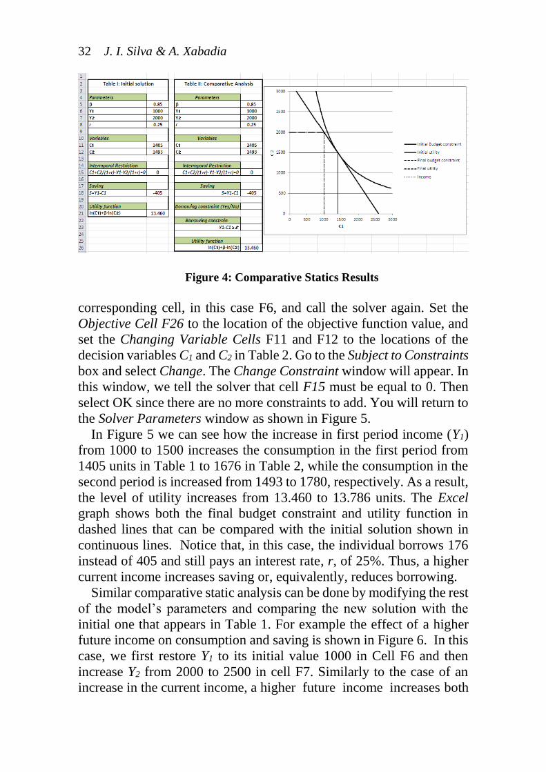
Figure 4.

Higher Present Income, Y1 , and Future Income, Y2

Now we can start by modifying present income Y1. In this case, we need

to include the new value of the present income parameter in the


Figure 4: Comparative Statics Results

corresponding cell, in this case F6, and call the solver again. Set the

Objective Cell F26 to the location of the objective function value, and

set the Changing Variable Cells F11 and F12 to the locations of the

decision variables C1 and C2 in Table 2. Go to the Subject to Constraints

box and select Change. The Change Constraint window will appear. In

this window, we tell the solver that cell F15 must be equal to 0. Then

select OK since there are no more constraints to add. You will return to

the Solver Parameters window as shown in Figure 5.

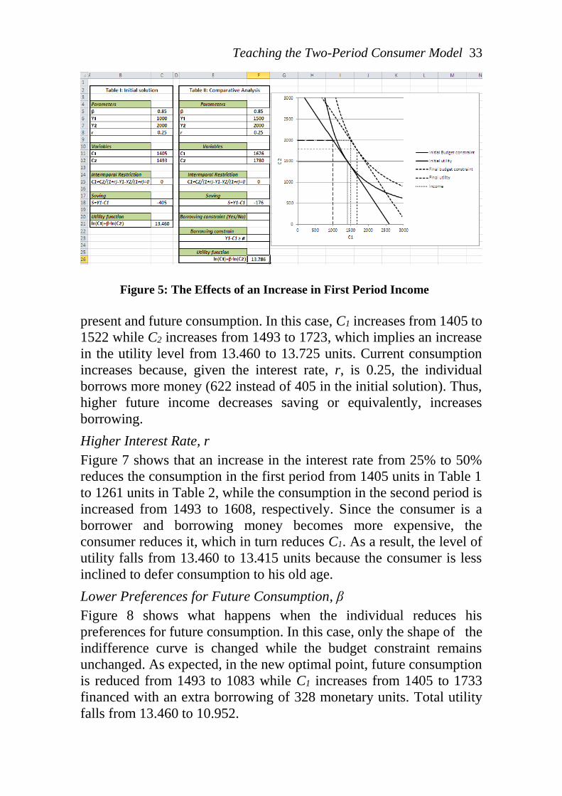
In Figure 5 we can see how the increase in first period income (Y1)

from 1000 to 1500 increases the consumption in the first period from

1405 units in Table 1 to 1676 in Table 2, while the consumption in the

second period is increased from 1493 to 1780, respectively. As a result,

the level of utility increases from 13.460 to 13.786 units. The Excel

graph shows both the final budget constraint and utility function in

dashed lines that can be compared with the initial solution shown in

continuous lines. Notice that, in this case, the individual borrows 176

instead of 405 and still pays an interest rate, r, of 25%. Thus, a higher

current income increases saving or, equivalently, reduces borrowing.

Similar comparative static analysis can be done by modifying the rest

of the model’s parameters and comparing the new solution with the

initial one that appears in Table 1. For example the effect of a higher

future income on consumption and saving is shown in Figure 6. In this

case, we first restore Y1 to its initial value 1000 in Cell F6 and then

increase Y2 from 2000 to 2500 in cell F7. Similarly to the case of an

increase in the current income, a higher future income increases both


Figure 5: The Effects of an Increase in First Period Income

present and future consumption. In this case, C1 increases from 1405 to

1522 while C2 increases from 1493 to 1723, which implies an increase

in the utility level from 13.460 to 13.725 units. Current consumption

increases because, given the interest rate, r, is 0.25, the individual

borrows more money (622 instead of 405 in the initial solution). Thus,

higher future income decreases saving or equivalently, increases

borrowing.

Higher Interest Rate, r

Figure 7 shows that an increase in the interest rate from 25% to 50%

reduces the consumption in the first period from 1405 units in Table 1

to 1261 units in Table 2, while the consumption in the second period is

increased from 1493 to 1608, respectively. Since the consumer is a

borrower and borrowing money becomes more expensive, the

consumer reduces it, which in turn reduces C1. As a result, the level of

utility falls from 13.460 to 13.415 units because the consumer is less

inclined to defer consumption to his old age.

Lower Preferences for Future Consumption, β

Figure 8 shows what happens when the individual reduces his

preferences for future consumption. In this case, only the shape of the

indifference curve is changed while the budget constraint remains

unchanged. As expected, in the new optimal point, future consumption

is reduced from 1493 to 1083 while C1 increases from 1405 to 1733

financed with an extra borrowing of 328 monetary units. Total utility

falls from 13.460 to 10.952.


Figure 6: The Effects of an Increase in Second Period Income

Figure 7: The Effects of an Increase in the Interest Rate

(b) The Borrowing Constraint

Until now we have assumed that the consumer can borrow as well as

save. The ability to borrow allows current consumption to exceed

current income. When the consumer borrows, he consumes some of his

future income today. Yet for many people such borrowing is

impossible. For example, an unemployed person wishing to buy a car

would probably be unable to finance this consumption with a bank loan.

Let’s, therefore, solve the model under a situation where the consumer

cannot borrow. The inability to borrow prevents current consumption


Figure 8: Effects of an Increase in Preference for Current Consumption

from exceeding current income. A constraint on borrowing can

therefore be expressed as:

𝑆 = 𝑌1 − 𝐶1 ≥ 0 (11)

This inequality states that consumption for the consumer must be less

than or equal to his income (period one). This additional constraint on

the consumer is called a borrowing constraint or, sometimes, a liquidity

constraint. We next introduce this constraint into the optimization

problem (5):

max𝐶1,𝐶2

𝑈(𝐶1, 𝐶2) = ln(𝐶1) + 𝛽 ln(𝐶2) (12)

subject to

𝐶1 + 𝐶2 (1 + 𝑟)⁄ = 𝑌1 + 𝑌2 (1 + 𝑟)⁄ and

𝑆 = 𝑌1 − 𝐶1 ≥ 0

Solving the model analytically under the scenario of borrowing

constraint is not straightforward as in (5). In this case, more advanced

methods may be required to solve this problem. Fortunately, Excel-

Solver can solve the problem by introducing a new restriction to the

optimal problem.

In excel, we say “Yes” to the borrowing constraint condition in cell

F20 and introduce this new restriction in cell F23 of Table 2. Then, we

add this constraint in Excel-Solver by Clicking on the Subject to


Figure 9: Setting Up the Borrowing Constraint Problem

Figure 10: Solving the Borrowing Constraint Problem

Constraints box and select Add. The Add Constraint window will

appear. In this window, we tell the solver that cell F23 must be higher

than or equal to 0 and select OK (there are no more constraints to add).

It will return to the Solver Parameters as in Figure 9. In the Solver

Parameters window click Solve. A window will appear telling us that

Solver has found a solution. Select Keep Solver Solution and click OK.


We have solved the consumer optimization problem under a borrowing

constraint as shown in Figure 10. Since the borrowing constraint is

binding in this case, first-period consumption equals first-period

income. The level of utility is reduced from 13.415 to 13.369 units

because the consumer would like to borrow to consume more in the first

period (as Table 1 shows) but he is not able to do it. Finally, the Excel

graph shows that there is a corner solution. Notice that, the final budget

constraint (dashed line) indicates that C1 cannot be higher than 1000

units.

5. CONCLUSION

The accessibility and flexibility of Excel spreadsheets gives economics

instructors a great tool to complement the traditional analysis of

economic problems. With this tool, applications that avoid long and

tedious calculations can be easily designed to enhance meaningful

learning. In this paper we have shown how to solve the basic two-period

consumer choice model using a spreadsheet and Excel-Solver and

illustrated the problem using an example from Mankiw’s

macroeconomics textbook. While completing the proposed exercise,

students can explore the main features of the model and learn key

concepts in a more dynamic and interactive way.

REFERENCES

Abel, A., Bernanke, B. and Croushore, D. (2010) Macroeconomics, Seventh

Edition, New York: Pearson Education.

Barreto, H. (2009) Intermediate Microeconomics with Excel, Cambridge:

Cambridge University Press.

Burda, M. and Wyplosz, C. (2009) Macroeconomics: A European Text, Fifth

Edition, Oxford: Oxford University Press.

Gilbert, J. and Oladi, R. (2011) “Excel Models for International Trade

Theory and Policy: An Online Resource”, Journal of Economic

Education, 42 (1), p.95.

Holger, S. (2004) “Solving Rational Expectations Models Using Excel”,

Journal of Economic Education, 35 (3), pp.269-283.

Houston, J. (1997) “Economic Optimisation using Excel's Solver: A

Macroeconomic Application and Some Comments Regarding Its

Limitations”, Computers in Higher Education Economics Review, 11 (1),

pp.2-5.

Mankiw, G. (2003) Principles of Macroeconomics, Fifth Edition, Boston,

Massachusetts: South-Western College Publishers.


Mankiw, G. (2011) Principles of Macroeconomics, Sixth Edition, Boston,

Massachusetts: South-Western College Publishers.

MacDonald, Z. (1996) “Economic Optimisation: An Excel Alternative to

Estelle et al.'s GAMS Approach”, Computers in Higher Education

Economics Review, 10 (3), pp.2-5.

Mixon, J.W. and Tohamy, S. M. (1999) “The Heckscher-Ohlin Model with

Variable Input Coefficients in Spreadsheets”, Computers in Higher

Education Economics Review, 13 (2), pp.4-6.

Nævdal, E. (2003) “Solving Continuous-Time Optimal-Control Problems

with a Spreadsheet”, Journal of Economic Education, 34 (2), pp.99-122.

Strulik, H. (2004) “Solving Rational Expectations Models Using Excel”,

Journal of Economic Education, 35 (3), pp.269-283.

Varian, H. (2006) Intermediate Microeconomic: A Modern Approach, Fifth

edition, New York: W.W Norton & Company.

teaching the two-period consumer choice model with …

Documents