team benchmarks - operafea€¦ · we use the finite element method and opera-3d elektra/ss to ......

TEAM Benchmarks

Problem 15:

Non-Destructive Evaluation

www.cobham.com/technicalservices

Problem Description1

This benchmark involves the calculation of the impedance change in a single air-cored AC coil above a thick

conducting plate due to the presence of a rectangular slot in the plate. We calculate the change in impedance as the

coil is scanned from the centre of the slot to a point far away; the direction of motion is along the long dimension of the

slot.

We simulate two cases: a low frequency drive, where the skin depth is large compared to the width of the slot, and a

high frequency case where the slot width and skin depth are comparable. The dimensions of the plate and slot are the

same in both cases. The dimensions of the coil differ between the two cases. We have ignored the specified errors on

the dimensions and used the central value.

Table 1: Dimensions of the plate and defect. These values are the same in both experiments.

The defect

Length (mm) 12.6

Depth (mm) 5.00

Width (mm) 0.28

The test specimen

Conductivity (S/m) 3.06e7

Thickness (mm) 12.22

The extent of the plate in the other two dimensions is unspecified in the benchmark description. We have chosen a

length of 150mm in each direction. This is to ensure that effects from eddy current confinement at the edge of the

plate do not impact on the results.

Figure 1: 3D model of the plate and defect.

1 This problem description is summarised from http://www.compumag.org/jsite/images/stories/TEAM/problem15.pdf

TEAM Benchmarks

Problem 15:



Experiment 1

The first experiment uses an air cored coil with dimensions:

Table 2: Dimensions for the coil in experiment 1.

The coil

Inner radius (mm) 6.15

Outer radius (mm) 12.4

Length (mm) 6.15

Number of turns 3790

Lift-off (mm) 0.88

The coil is driven by a 50V AC supply at 900Hz and connected to a 100 Ohm resistor. No resistance is imparted by

the coil itself in the simulation. The supply voltage, circuit resistance and coil current are not specified by the

benchmark problem, nor are they required to be; this configuration is used so that a circuit equation method may be

used to obtain the impedance. The precise values used are not relevant as all materials in the model have linear

properties: were any material properties nonlinear, we would need to use the same circuit configuration as the test.

Figure 2: Meshed model for experiment 1. Surrounding air volumes are hidden.

TEAM Benchmarks

Problem 15:



Experiment 2

The second experiment uses an air cored coil with dimensions:

Table 3: Dimensions for the coil in experiment 2.

The coil

Inner radius (mm) 9.34

Outer radius (mm) 18.4

Length (mm) 9.0

Number of turns 408

Lift-off (mm) 2.03

The coil circuit is configured as in Experiment 1.

Figure 3: Meshed model for experiment 2. Surrounding air volumes are hidden.

Note that the air volume surrounding the coil in this experiment has been given a larger mesh size than in experiment

1. This in turn alters the mesh size in the surface layers of the plate beneath the coil. We discuss the effect of this

later on.

TEAM Benchmarks

Problem 15:



Solution Method The description is of a steady-state AC problem. We use the finite element method and Opera-3d ELEKTRA/SS to

solve the field distributions. By connecting the coil to a circuit we make available the complex voltage and current,

which we then use to calculate the resistive and inductive impedance in each model. If we look at the phase angle

where V contains only the real component = + 0 and ignoring capacitance, we can show that2:

= − ∙ + =

+

The solution is calculated both with and without the presence of a defect in the plate, and the difference in the

inductance and resistance is determined.

We can also look at the magnitude and phase of the change in impedance:

|∆| = ∆ + ∆∆ = tan ∆∆ !

where ∆ = ∆.

Model Description We use the Opera-3d Modeller’s scripting capabilities to create the model for each experiment. The script is

parameterised so that either experiment can be created from the same script file. A control loop is used to translate

the coil to each successive position, generate the mesh and create the solution file.3

Each solution file contains two simulations: one where the defect has the same material properties as the surrounding

plate (simulating a plate with no defect), and one where the defect has the properties of air. This allows us to ensure

that both simulations are using the same mesh, and so any calculated change in the impedance is due to the

presence of the defect and not a change in the mesh itself, due either to adding the slot or moving the coil. This

technique was first suggested by Dr Larry Turner from Argonne National Laboratory – see L. R. Turner, “Solving

TEAM Problem 8 (Slot in a Plate) on a PC with ELEKTRA”, TEAM Workshop, Okayama University, Okayama, Japan,

March 21, 1996

2 See the Opera ASK, “Calculation of Inductance in Time Harmonic Solutions” 3 As the model is already parameterised a second method would be to add an additional parameter, the centre

position of the coil, and use the Opera Optimizer to perform a grid sweep over coil positions. The advantage of this is

that the model rebuild stage can then also be handed off to the batch queue system along with the solution stage and

post-processing. As the Optimizer is a separately licensed product we do not use this method here, so that this paper

is as widely applicable as possible.

TEAM Benchmarks

Problem 15:



Tetrahedral meshing is used throughout (except in the conductors, see below). Opera-3d allows surfaces to be

layered – the marked surface is copied and translated a specified distance and number of times. The mesh on each

copy is guaranteed to be identical; this permits higher aspect ratio tetrahedral elements than would normally be

considered good finite element practice as it generates a more regular mesh between the face copies.

At high frequencies the skin depth is small; this can make creating a suitable mesh difficult even with layering of

tetrahedral elements. Opera-3d can also use hexahedral elements (as well as triangular prisms and pyramids) which

can give good results even at very high aspect ratios. In this example we have decided to utilise the same model and

mesh as far as possible for both experiments. To overcome the problem of the small skin depth in Experiment 2, we

apply a Surface Impedance Boundary Condition (SIBC) to the material properties of the conducting volumes. This

formulation treats all the current as flowing on the surface of the material, and negates the need for field solutions

within the volume. There is therefore no need to capture the skin depth explicitly in the mesh.

Opera has several methods for representing coils:

1. Fixed-current coils can be modelled as being distinct from the mesh, providing only a fixed drive to the model.

Using this method does not allow the calculation of circuit parameters; inductance values can still be

determined from flux linkage or stored energy methods, but any resistance in the coil would need to be

calculated manually. (Note that, in the model, the wire resistance will be taken as zero, so the only resistive

terms in the impedance come from the resistance of the plate and the bulk resistor in the circuit.)

2. Coils may be modelled using filamentary representations. Coils modelled in this way may be connected to

circuits, and the filaments become edges within the finite element mesh. The current is treated as flowing only

in these filaments, and so the field solutions around the filaments themselves are rarely smooth. This method

is useful where coils are thin or are not themselves the region of interest.

3. The coil volume itself can be meshed. This provides several benefits: the coils become independent volumes

which can be utilised in post-processing; current is treated as being uniformly distributed throughout the coil

cross-section, so field patterns are smooth and accurate in the coil region; meshed coils can be connected to

circuits, allowing calculation of inductance and resistance from circuit parameters.

From the above descriptions, it is clear that meshed coils are the most appropriate for this solution. All Opera

conductors are defined in such a way that the generated volumes are hexahedral and can be meshed as such. We

make use of this facility in all the models simulated below.

The models have reflection symmetry (tangential magnetic) in the ZX-plane at all positions of the coil. We utilise this

symmetry in order to reduce the size of the models to be solved.

TEAM Benchmarks

Problem 15:



Model Verification The problem description also provides the isolated coil inductance for both experiments. We can use this to verify that

our initial model is sufficiently well meshed and that our post-processing method is correct. We use the same mesh as

we will use in the later stages, but with all material properties set to those of air to simulate the coil isolated in free

space. The isolated coil inductance is shown in

Coil Inductance Measured (mH) Calculated (mH) Difference (%)

Experiment 1 221.8 ± 0.04 224.1 1.04

Experiment 2 3.96 ± 0.1 3.9624 0.06

From these results, it is clear that our mesh is adequate to support the inductance calculations. Note of course that

this says nothing about the suitability of the mesh to capture the eddy currents, as the conductivity is zero in these

verification models.

Experimental Errors The results of the Opera-3d simulations are shown below and compared to measured data as provided in the

description of the TEAM problem. Experimental errors, as described in the benchmark, are:

Error in ∆L Error in ∆R

Experiment 1 0.04 mH 0.1 Ω

Experiment 2 0.02 µH 0.1 Ω

Note that the units for ∆L in Experiment 2 are listed in the paper as being mH. This is inconsistent with the error

estimate and the isolated impedance of the coil: the correct units are µH.

TEAM Benchmarks

Problem 15:



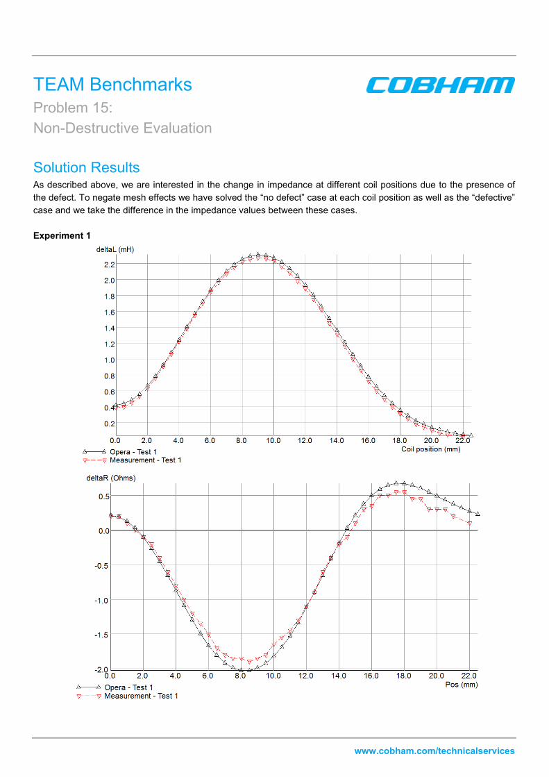
Solution Results As described above, we are interested in the change in impedance at different coil positions due to the presence of

the defect. To negate mesh effects we have solved the “no defect” case at each coil position as well as the “defective”

case and we take the difference in the impedance values between these cases.

Experiment 1

TEAM Benchmarks

Problem 15:



TEAM Benchmarks

Problem 15:



Experiment 2

TEAM Benchmarks

Problem 15:



TEAM Benchmarks

Problem 15:



Conclusions Opera performs consistently well across both experiments – deviation from the measured change in both inductance

and resistance are close to experimental error. The only major apparent difference is in the argument of the

impedance change in experiment 2; this can be explained, as the experimental error in ∆R for experiment 2 is

approximately 500% of the value of ∆R at the central position (0.0 mm) and beyond the end of the slot (30.0 mm). The

error in the argument for the experiment is therefore very large, and Opera is consistent within this range.

TEAM Benchmarks

Problem 15:



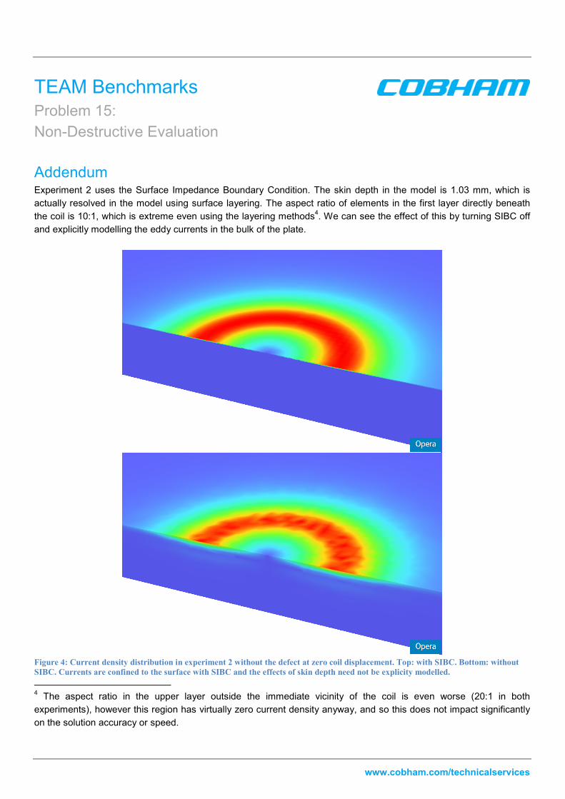
Addendum Experiment 2 uses the Surface Impedance Boundary Condition. The skin depth in the model is 1.03 mm, which is

actually resolved in the model using surface layering. The aspect ratio of elements in the first layer directly beneath

the coil is 10:1, which is extreme even using the layering methods4. We can see the effect of this by turning SIBC off

and explicitly modelling the eddy currents in the bulk of the plate.

Figure 4: Current density distribution in experiment 2 without the defect at zero coil displacement. Top: with SIBC. Bottom: without

SIBC. Currents are confined to the surface with SIBC and the effects of skin depth need not be explicity modelled.

4 The aspect ratio in the upper layer outside the immediate vicinity of the coil is even worse (20:1 in both

experiments), however this region has virtually zero current density anyway, and so this does not impact significantly

on the solution accuracy or speed.

TEAM Benchmarks

Problem 15:



Note the variation of the current density distribution on the upper surface of the plate. This is the beginning of

breakdown in the solution, and will become more pronounced as the frequency is increased. At this stage, the results

of the impedance calculations have not yet broken down, as the results below show, but they will become increasingly

inaccurate as the frequency increases. Experiment 1 uses a smaller mesh size in the air volume surrounding the coil.

This affects the mesh size in the layers of the plate; Experiment 1 has an aspect ratio of 5:1 in this region, which is

just about acceptable when using surface layering. Further refinement of the meshing would most likely improve the

results in all cases.

Using the SIBC helps to overcomes these difficulties. Although we have used the same (extreme aspect ratio) mesh,

the solution quality is already greatly improved. Current density within the volume of the plate is not explicitly

calculated. In fact, we can remove all layering in the surface and around the defect and obtain excellent results using

SIBC.

Figure 5: Experiment 2 model with all layering removed.

TEAM Benchmarks

Problem 15:



TEAM Benchmarks

Problem 15:



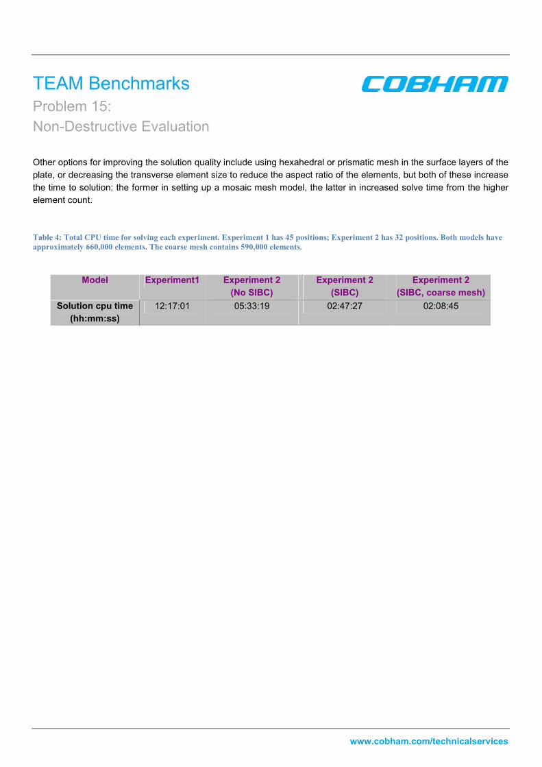
Other options for improving the solution quality include using hexahedral or prismatic mesh in the surface layers of the

plate, or decreasing the transverse element size to reduce the aspect ratio of the elements, but both of these increase

the time to solution: the former in setting up a mosaic mesh model, the latter in increased solve time from the higher

element count.

Table 4: Total CPU time for solving each experiment. Experiment 1 has 45 positions; Experiment 2 has 32 positions. Both models have

approximately 660,000 elements. The coarse mesh contains 590,000 elements.

Model Experiment1 Experiment 2

(No SIBC)

Experiment 2

(SIBC)

Experiment 2

(SIBC, coarse mesh)

Solution cpu time

(hh:mm:ss)

12:17:01 05:33:19 02:47:27 02:08:45

team benchmarks - operafea€¦ · we use the finite element method and opera-3d elektra/ss to ......

Documents