tec rep mri 54 - mri-jma.go.jp · even in this case the average 85kr activity concentration over a...

1

TECHNICAL REPORTS OF THE METEOROLOGICAL RESEARCH INSTITUTE No. 54

1. Introduction

The radioactive noble gas 85Kr is a beta emitter with a half-life of 10.76 years. Natural

85Kr is produced by nuclear reactions by cosmic radiation in the upper atmosphere and

spontaneous fission of the heavy elements in the Earth’s crust (Styra and Butkus, 1991).

However most of the 85Kr in the present atmosphere is derived from anthropogenic

sources (i.e., nuclear weapons tests, nuclear-fuel reprocessing plants and nuclear reactors).

At present, the major sources of atmospheric 85Kr are releases from the nuclear fuel

reprocessing plants in Europe (Rath, 1988, Von Hippel et al., 1986, Weiss et al., 1986 and

1992).

The relatively well-known distribution of the point like sources and the fact that the only

significant sink in the atmosphere is radioactive decay, make 85Kr an ideal tracer to assess

the characteristics of the large-scale horizontal and the interhemispheric transport, as

depicted in numerical atmospheric circulation models. For instance Jacob et al. (1987),

Zimmermann et al. (1989) and Draxler (2007) simulated the global 85Kr distribution using

a three-dimensional tropospheric model while Rath (1988) used a two-dimensional model.

The solubility of 85Kr (as with all inert gases) in water is very low (the ratio of stable

Kr to water is 1.85x 1010 g/g at equilibrium) and therefore the ocean dissolves not more

than 0.1% of the annual input of 85Kr (Izrael et al., 1982). However 85Kr is also a very

useful tracer to have better understanding of oceanic processes such as relatively short-term

(decadal) atmosphere-ocean exchanges and the determination of the age distribution of

water masses in the ocean as described by Loosli (1992). The 85Kr distribution in the

atmosphere can also be used as an indicator of clandestine separation of plutonium for

building nuclear weapons.

2


Because of its inertness, the major sink of 85Kr in the Earth’s surface is a radioactive

decay at the rate of about 6% per year. The imbalance between sinks and sources of 85Kr

causes a change in the atmospheric 85Kr global inventory. The current global inventory of

85Kr in the atmosphere is estimated to be 5000 PBq (Hirota et al., 2004). Thus, 300 PBq of

85Kr has been lost each year from the atmosphere, due to its radioactive decay. However,

the amount of released 85Kr from the nuclear-fuel reprocessing plants in Europe is now 300

to 400 PBq per year United Nations, 2000). In fact the atmospheric 85Kr activity

concentration is increasing yearly according to the differences between released 85Kr and

decayed 85Kr (Hirota et al., 2004; Igarashi et al., 2000; Pollard et al., 1997).

Owing to its long half-life and chemically inertness, 85Kr has spread all over the globe.

The activity concentration of 85Kr in ground level air of 1.3 Bq m-3 in 1999 at mid-latitudes

of the Northern Hemisphere is slowly but continuously increasing at an annual rate of 30

mBq m-3 because the annual global release rate of 85Kr to the atmosphere still exceeds the

removal rate by decay. Therefore it is important to monitor the concentration of

atmospheric 85Kr in order to evaluate potential radioecological impacts on human health

and the environment. Regarding radiation protection, based on its small effective dose

conversion factor of the order of nSv yr-1 per Bq m-3, the annual dose of 85Kr received by

the general public is insignificant compared with the annual external dose from natural

sources. In the vicinity of a nuclear-fuel reprocessing plant the 85Kr activity concentrations

sometimes reach values of some hundred thousand Bq m-3 for a short period of time

(Gurriaran et al., 2004). Even in this case the average 85Kr activity concentration over a

year would not reach the proposed ICRP dose limit (Fujitaka, 1995). From the viewpoint

of the atmospheric sciences 85Kr data can be used for validation of local, regional and

global transport models. The well-known source term and its chemically inert properties

3


make 85Kr a useful tool for atmospheric studies (Weiss et al., 1986, 1987, 1992) in which

transport and dilution processes should be considered but no complicated chemical

reactions are involved. In addition it seems possible to detect clandestine plutonium

production for nuclear weapons by monitoring 85Kr (Sittkus and Stockburger, 1976,

Kalinowski et al., 2004, World Meteorological Organization, 1996). As an environmental

effect the contribution of 85Kr to air conductivity has been discussed (Styra and Butkus,

1991; Stockburger et al., 1977), although the contribution of 85Kr at background

concentration levels is concluded to be much smaller than the natural ones and to be buried

in natural fluctuations. However, attention should be given to the fact that the background

level of the atmospheric 85Kr activity concentration at the global level is still increasing.

At the Meteorological Research Institute (MRI) in Tsukuba, Japan, atmospheric 85Kr

activity concentrations have been observed since 1995 in collaboration with the Bundesamt

für Strahlenschutz (BfS), Germany (Igarashi et al., 2000). Igarashi et al. (2001) developed

a 85Kr measuring system based on the BfS method in 2000. Details of the method and the

techniques developed and used by the BfS to monitor the activity concentrations of 85Kr

and 133Xe are described in Stockburger et al., 1977 and in Sartorius et al. 2002. It was

confirmed by intercomparison measurements between the BfS and the MRI laboratories

that the 85Kr activity concentration measured by the MRI system is traceable to the value

determined by the BfS. (Igarashi et al., 2001, Figure 8, see appendix 4)

In 2006 the MRI and the Japan Chemical Analysis Center (JCAC) conducted a

cooperative research program of 18 months to develop a practical 85Kr measuring system

based on the MRI system. The objectives of this program were to establish a monitoring

system of atmospheric 85Kr in Japan and to publish a technical document on 85Kr

measurements.

4


In this technical report we describe the 85Kr measurement system and report the results

of 10 years of observation of 85Kr in Tsukuba, Japan.

5


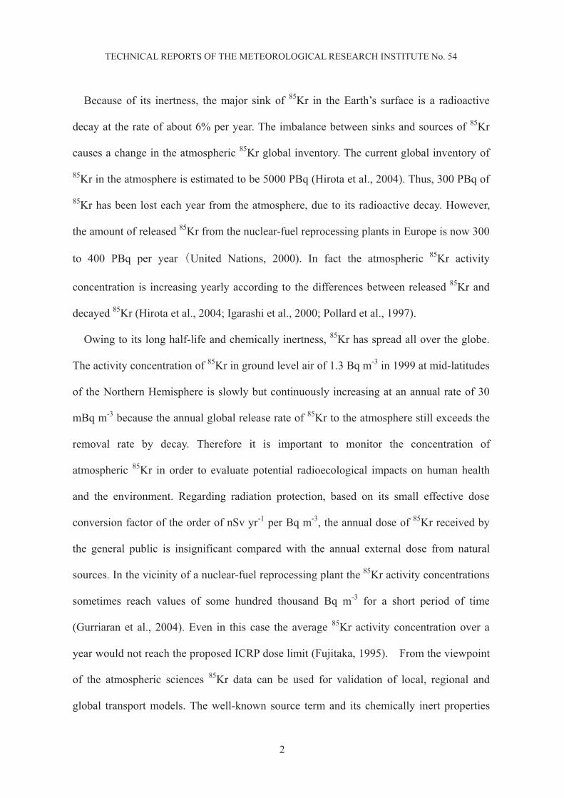
2. Instruments of cold charcoal trap - gas chromatography - gas

counting system of 85Kr

In this chapter we describe the sampling procedures, including a sampling apparatus

(cold charcoal trap), and the determination of 85Kr activity concentration by a combined

gas chromatography and gas counting system as well as the description of the

instrumentation.

Figure 2.1 Schematic diagram of the 85Kr measurement system

2.1 Sampling procedures

2.1.1 Outline

Atmospheric krypton is collected using a sampling apparatus (Fig. 2.2) that consists of

an air pump, a metal absorber, and a liquid nitrogen dewar bottle. First the air is passed

through a glass filter (Whatman GF/F 47mmØ) to remove dust, and then dehumidified with

a refrigerator or a dehumidifier. After removal of dust and water vapor the air is passed

through a metal absorber, which is immersed in a liquid nitrogen dewar using the air pump

and the atmospheric Kr is trapped on the activated charcoal that fills the lower part of the

absorber. Air sampling is continuously performed for one week at a constant flow rate of 1

6


l min-1 and about 10 m3 of the air is introduced into the absorber during the routine

sampling period. After end of collection trapped moisture is removed from the absorber,

and the absorber is heated to desorb the Kr trapped on the activated charcoal. The Kr

fraction is completely transferred by expansion into an evacuated aluminum bottle

followed by rinsing the absorber and the tubing with pressurized He gas at the end of the

desorption step.

Figure 2.2 Diagram of sampling apparatus

The sampling procedure described below is based on the techniques and methods of the

BfS, except for using refrigerator or a dehumidifier to remove moisture due to high

humidity of the air in Japan. The metal absorber (Fig. 2.3) was developed and designed at

the BfS (Sartorius et al. 2002, BfS 2004). It is cylindrical, 63cm and 6cmØ in length and in

radius, respectively. The absorber has a needle valve, a stopcock, a manometer and a safety

valve. The air flow rate through the absorber is regulated with a needle valve installed at

the entrance of the absorber. Atmospheric Kr trapped on the activated charcoal is

7


transferred to an aluminum bottle by opening the stopcock at the outlet side of the absorber.

The pressure in the absorber can be read by the manometer. When the pressure in the

absorber exceeds +0.5 MPa, the excess pressure is automatically blown off through the

safety valve. The upper part of the absorber internal volume has plenty of metal fins to

remove from the air moisture as ice and CO2 as dry ice. The lower part of the absorber

internal volume is filled with 200 g of activated charcoal (No. 1.09631.0500, 0.3-0.5 mm

(35-50 mesh), Merck, Germany). Atmospheric trace constituents with low melting points

(e.g., Kr and Xe) are adsorbed on the activated charcoal at liquid nitrogen temperature. The

absorber is kept at low pressure (about 0.5 atm) during sampling to avoid the condensation

of the main air constituents N2 and O2. The major part of the air passed through the

absorber is discharged by the air pump.

Figure 2.3 Absorber for 85Kr sampling 1: Quick connects (sample out), 2: Quick connects (sample in), 3: Needle valve, 4: Safety valve, 5: Manometer, 6: Stop cock, 7: Fin, 8: Activated charcoal.

8


After collection, the absorber is warmed to room temperature. In this step, most of the

gaseous air components (N2, O2 and CO2) and the water are discharged from the absorber.

The Kr trapped on the activated charcoal is transferred into an evacuated aluminum bottle

(minican) by heating the absorber up to 300 ºC. Last of all the transfer is completed by

sweeping the absorber and the tubings with He gas and flush the gas into the aluminium

bottle at a pressure of 0.4 MPa. The aluminum bottle has a volume of about 1 l with a

spring-type valve. Usually, this spring-type valve seals the aluminum bottle. When the

spring-type valve is pushed with a thin stick, the spring can be depressed downward and

the gas sample can be introduced into the aluminum bottle. The aluminum bottle can be

covered with a cap to protect the valve. This lightweight but strong bottle is a suitable

transportation container, and the gas sample can be preserved for a long period.

2.1.2 Start of sampling

To start sampling, fix the air inlet tube carefully to the outside wall of a building to avoid

rainwater. Fresh air should be collected to ensure that the sample represents 85Kr activity

concentration in the atmosphere. During storage the absorber is kept under He pressure at

+0.4 MPa. Before start of sampling the absorber is depressurized to atmospheric pressure

by opening the stopcock at the outlet. Afterwards the stopcock is closed and the needle

valve checked if its closed correctly. Attach the fixing rubber collar to the absorber and

cool it in the liquid nitrogen dewar. Make sure approx. 10 cm of the stainless steel part of

the absorber is above the top of the liquid nitrogen dewar. The screw bolt to exchange the

activated charcoal is fitted on the bottom of the absorber. Any shocks may affect the air

tightness of the absorber. Therefore, the handling of the absorber has to be paid care. In

order to avoid that moisture in the air sticks on the surface of the absorber as ice and to

9


control the liquid nitrogen evaporation, it is required that the absorber is covered by a

thermal insulator on the part of the fixing rubber collar. When the absorber is cooled by the

liquid nitrogen, the activated charcoal firstly acts as a cryopump, and therefore the pressure

of manometer is gradually decreased. The pressure of manometer will be constant, when

the gas adsorption on the activated charcoal will be reached saturation. Connect the tubes

to the absorber and turn on the flow meter. After the pressure of the manometer reached

-0.06 MPa open the needle valve and adjust the flow rate to 1.00 l min-1. Ten minutes later,

turn on the air pump and open the stopcock completely.

2.1.3 Routine work during sampling

During sampling check the gauges (manometer, gauge1 and gauge2), flow rate, total air

volume, and amount of remaining liquid nitrogen daily. Make sure that the pressure of the

manometer is below -0.03 MPa, that the gauge1 constantly indicates the atmospheric

pressure, and that gauge2 constantly indicates the negative pressure. It is important that the

flow rate shows 1.00 l min-1. When the flow rate is lower adjust the flow rate back to 1.00 l

min-1 by opening the needle valve. The total amount of the air volume would be 1.44 m3

per day.The consumption rate of liquid nitrogen is 3 to 5 kg per day, so refill the dewar

with liquid nitrogen every two days. Due to the large thermal capacity of the absorber, its

increase of the temperature is negligible if the absorber is taken out of liquid nitrogen

dewar during the short time of refilling. But it is better to immerse the absorber into a spare

liquid nitrogen dewar when refill the engaged dewar with liquid nitrogen.

2.1.4 Exchange of the absorber

At the end of the collection period close the stopcock and the needle valve of the

10


absorber in use and turn off the air pump. Disconnect the tubes from the absorber, take it

out of the dewar and remove the rubber collar from the absorber. Turn the absorber upside

down and hold it in a stand (refer to Fig. 2.4). When the pressure in the absorber has been

above atmospheric pressure (it takes about 5 minutes), open the stopcock completely and

leave it for 35 minutes. During this time the main air components adsorbed on the activated

charcoal are discharged. We determined that 1-2 % of Krypton had lost during a one hour

warming up. In case the stopcock has not been opened when warming up the absorber to

room temperature, the pressure in the absorber increases over +0.5 MPa, the safety valve is

automatically opened and the pressure in the absorber is immediately decreased. Exchange

a glass filter of the sample unit and refill the dewar with liquid nitrogen. Finally start the

next sampling with the other absorber as described in chapter 2.1.2 “Start of sampling”.

Figure 2.4 Removal of water from absorber

11


2.1.5 Transfer Kr to aluminum bottle

Close the stopcock of the upside down absorber and leave it stand again for one hour to

dissolve the ice trapped in the absorber. The pressure in the absorber increases to +0.2 MPa

due to the desorption of air trapped on the activated charcoal. If the pressure in the

absorber is less than +0.04 MPa, pressurize it with He gas to +0.1 MPa. Rotate the absorber,

which is turned upside down, like a top, attach the Quick-connects (Swagelok®) to the port

of the needle valve, open the needle valve and allow the water, trapped in the absorber, run

out dropwise into a beaker. Recording the amount of water can help determine whether the

moisture trap in the absorber is operating correctly or not.

After the pressure of the absorber reaches atmospheric pressure close the needle valve,

remove the Quick-connects and insert the absorber into a cylindrical heater. When the

sample gas is transferred into the aluminum bottle, use a water adsorbent tube to remove

the water vapor in the sample gas (Figures.2.5 and 2.6). Fill the inner tube of the water

adsorbent tube with the regenerated silica gels, insert it into the outer tube, and connect it

firmly to the upper cap of the water adsorbent tube with the stretching ring. The water

adsorbent tube is connected between the absorber and the aluminum bottle. When the water

adsorbent tube is assembled no silica gel should remain on the surface of the flange of the

inner tube.

12


Figure 2.5 Water adsorbent tube

Figure 2.6 Transfer of sample gas

13


Screw a closed minican valve onto an evacuated aluminum bottle (minican), and connect

it to the water adsorbent tube with Quick-connects. Connect the counter-port of the water

adsorbent tube to the absorber with the Quick-connects. Open the stopcock and the minican

valve completely ensure that the manometer indicates negative pressure (-0.03 MPa) and

then record it. Close both valves and switch on the heater. Heat the absorber for one hour at

300 ºC. Fifteen minutes after the heater was switched on check the manometer to make

sure that no sharp increase of the pressure has occurred due to the water vapor. Open the

stopcock and the minican valve completely to decrease the pressure of the system to

constant pressure. After the stabilisation of the pressure in the system close both valves.

After one hour open the stopcock and the minican valve completely and record the pressure

of the manometer. The pressure of the gases in the minican is typically +0.1 - +0.3 MPa. To

ensure a quantitative transfer of the desorbed gases from the activated charcoal to the

aluminum bottle, rinse out the absorber by slowly pressurizing the system with He gas

from the port of the needle valve side until +0.4 MPa is reached. After pressurizing at +0.4

MPa, close all the valves and remove the water adsorbent tube (including the minican

valve and the aluminum bottle) from the absorber. Remove the minican valve (including

the aluminum bottle) from the water adsorbent tube. Remove the aluminum bottle from the

minican valve. Paste a sampling label on the bottle indicating the sampling location, the

sampling period, and the sample number and then screw a cap onto the bottle.

2.1.6 Re-use of sampling instruments

a. Regeneration of the absorber

Connect a silicon tube to the outlet port of the stopcock side and open it to exhaust the

excess pressure. At this time, water drops are attached inside the silicon tube. Blow He gas

14


into the absorber from the port of the needle valve side at a low flow rate. It is easy to

adjust the flow rate by controlling the out-coming gas using a conventional flow meter with

a water tube (at several bubbles per second). Continue to heat the absorber (300 ºC) until

no condensed water is visible in the silicon tube at the outlet (about one hour).

Next, switch off the heater and leave the absorber in the heater for two hours. Continue

to flush the absorber with He gas. After two hours close all the valves of the absorber,

remove it from the heater, place it on the stand and allow it to cool. After the absorber is

cooled to room temperature, pressurize it with He gas until +0.4 MPa is reached. Check the

air tightness of the absorber by appling soapy water to the parts where leakage would occur

making sure no bubbles appear. With the next usage of the absorber, air tightness can be

ensured by maintaining the pressure (+0.4MPa).

b. Ensuring dryness of the water adsorbent tube

Open the stretching ring, remove the inner tube and move the silica gel to a beaker. Next

regenerate the silica gel by heating it in a drying oven, dismantle the water adsorbent tube

and dry the components until the next usage.

2.1.7 Maintenance

If a suitable flow rate can not be achieved during sampling, it is necessary to confirm

that the air inlet has not been blocked. If the manometer has not maintained negative

pressure, make sure that no leakage is occurring in the sampling unit and that the air pump

has normal suction. If the air pump has failed, replace it with a spare air pump. If the

exchanged air pump is repaired, it can be reused.

If the flow rate is unstable, check the connection between the tubes and the sampling

unit. The activated charcoal in the absorber will become fine during use, and part of the

15


activated charcoal may flow out with water from the needle valve. Therefore, change the

activated charcoal every one or two years.

2.2 A brief system description

The MRI 85Kr measuring system consists of two trap tubes (made of stainless steel;

Traps 1 and 2, packed with activated charcoal), three gas chromatographs (GC 1, 2 and 3)

(GC-14B, Shimadzu, Kyoto, Japan), an activity measurement unit containing a gas-flow

proportional counter (200 ml in volume) (No. 49583, LND, New York, USA) and two data

processing and control systems (Shimadzu Chromatopack C-R7A). The sample flow lines

are built mostly of using stainless-steel tubes (1/8 inch or 2 mm diameter) and connected

by appropriate stainless-steel fittings (Swagelok, Solon, OH, USA and Shimadzu). The

treatment unit (Shimazu) is composed of Trap 1 [6 mm diameter, filling: 60 ml of activated

charcoal, 30 to 45 mesh (Shimadzu)] and a thermal conductivity detector (TCD; hereafter

referred to as TCD-P). This unit is used for the crude separation of Kr from other gases.

Figs. 2.7 and 2.8 show the schematic flow chart of pre-treatment unit and the GCs,

respectively. The separation and purification conditions of the whole system were adjusted

and calibrated by using simulated standard gas, which was designed to have a composition

similar to that of the real sample gas in the aluminum bottle. The pre-treatment unit has

multiple ports to introduce the simulated gas for test and calibration and He gas for purging

the line; their amounts and flow rates are controlled by a mass flow monitor/controller

(DS-3, Stech, Kyoto, Japan).

16


Figure 2.7 Schematic flow chart of pre-treatment unit

Figure 2.8 Schematic flow chart of the GCs

17


2.3 Analytical procedures

The sample gas in the aluminum bottle is injected into the pre-treatment unit (see Fig.

2.7); in the first stage, it sequentially passes through the wet CO2 removal column and the

water removal column. The wet CO2 removal column (22 mm in diameter, 230 mm in

length) has a special design to remove a large volume of CO2; packed with Askarite II (No.

C049-H40, 8-20 mesh, 50 g, Thomas Scientific, Swedesboro, NJ, USA), on the silica gel

layer (0.35 to 2.0 mm, 7 g) (Kanto Kagaku, Tokyo, Japan), with 10 ml of pure water added

just before the analysis. The water removal column (10 mm in diameter, 145 mm in length)

is packed with Mg(ClO4)2 (No. 500-94444, 10 g) (Kishida Chemical, Osaka, Japan). The

sample gas is pushed into the pre-treatment unit by over pressure in the aluminum bottle.

The gas flow rate is set at 250 ml min-1 for the sample and at 350 ml min-1 for the

simulated sample. The sample gas then flows into Trap 1 where it is cooled to -90 ºC by

immersion in refrigerated ethanol (5 liter). The refrigerator used is a Cryocool CC-100II

(Neslab, Portsmouth, NH, USA). After most of the sample gas is released in the aluminum

bottle by over pressure, He gas is charged into the aluminum bottle to rinse it and to

complete the sample transfer. The flush of pure He completely elutes major air components

adsorbed on the activated charcoal in Trap 1 chromatographically. It usually takes 30 to 40

min to elute most of the air components from Trap 1. Fifty to 60 minutes after the start,

Trap 1 is manually removed from the cold bath and placed in the heater (ARF-80KC, Asahi

Rika, Chiba, Japan). Continuous He flow at up to 400 ºC transfers the gases retained in

Trap 1 to Trap 2 (4 mm in diameter; filled with 1 ml of activated charcoal) immersed in

liquid Ar (about 0.5 l). After adsorption of Kr in Trap 2, the trap is heated by a sheath

heater, and the gases retained in the trap are injected sequentially into GC 1 and GC 2 for

isolation of Kr (Fig. 2.8). In these processes, pure CH4 (purity 99.999%) is used as a carrier

18


gas which is also used as part of the counting gas mixture in the proportional counter to

improve the counting conditions for the 85Kr activity measurement. The analytical

conditions for the GCs are summarized in Table 1 in Igarashi et al., (2001). In addition,

Trap 2 and GC 1, 2 and 3 are operated automatically by a Shimadzu Chromatopack C-R7A

system and its BASIC program. The chromatogram output data of all GCs are

automatically recorded and analyzed by the C-R7A.

The separation system at the Bundesamt für Strahlenschutz in Freiburg is based on two

large-diameter, column and valve. It operates under normal pressure and a low gas flow

rate of several milliliters per minute (Stockburger et al., 1977). The MRI separation system

is composed of commercially available GC parts, (i.e., small-diameter tube, column and

valve). It operates at relatively high pressures up to 300 kPa and a high gas flow rate of 70

ml min-1. This caused a problem in the early version of the MRI system. Even if CO2 were

completely removed, the separation column was saturated with abundant N2 and O2

relative to Kr in the sample, resulting in insufficient isolation and purification of Kr from

major air components. In the early stages of system development, removal of O2 was

attempted by using an oxidation reaction column, but a satisfactory outcome was not

obtained. Therefore, the idea of chemical removal of O2 was later rejected. A pre-treatment

unit, which employed gas chromatographic separation at low temperature, was newly

developed and integrated. Crude separation of Kr from N2 and O2 is carried out with this

unit, to achieve the complete isolation of Kr. This unit is the most innovative part of the

MRI system. Activated charcoal, which has a high affinity to noble gases heavier than Ar

was chosen as an adsorbent in this trap-and-purge technique. Trap 1 was also intended to

have a sufficiently large capacity (60 ml) to avoid saturation problems. In order to achieve

the chromatographic separation of N2 and O2 from the noble gas fraction, the retention time

19


of Kr at low temperature was monitored. A known volume of Kr was introduced into Trap

1 immersed in a different cold medium and its elution was recorded. The retention time

was increased to a good value by decreasing the column temperare. The retention time of

Kr was long enough to completely separate Kr from other gas components at 90 ºC. It was

also confirmed that the temperature for the purge procedure should be as high as possible

so as to ensure the recovery of the noble gas fraction from the trap. In practice, the purge

temperature was set at 400 ºC.

2.4 Gas counting system

The purified Kr fraction is subsequently introduced into the loop which includes the

proportional conter (Fig. 2.9). The loop is closed off after the Kr fraction has been

introduced and the sample gases in the loop are mixed well by circulation with a newly

devised plunger-type air pump (Mac pump 40, Nitto Koatsu, Ibaraki, Japan) in order to

attain homogeneity in the loop. When homogeneity has been achieved, the excess pressure

is released by equilibration with atmospheric pressure through a four-way valve in the loop.

The beta activity of 85Kr is counted by the proportional counter. Background counting is

carried out before and after the Kr sample measurement to confirm the sample purge. The

beta-counting of 85Kr is continued until at least 10000 net counts have been obtained. The

activity counting unit is composed of a NIM bin power module (Repic RPN-011), a

four-channel high-voltage supply (Repic RPH-011), a pre-amplifier (Model 142AH, Ortec,

Tennessee, USA), an analog-to-digital converter (Model 705, Philips Scientific, Mahwah,

NJ, USA), a gate and delay generator (Model 794, Philips Scientific), logics devices

(Models 756 and 757, Philips Scientific), and a personal computer support counter system

(RPN-032, Repic). Along with activity counting, the volume of stable Kr in the loop is

20


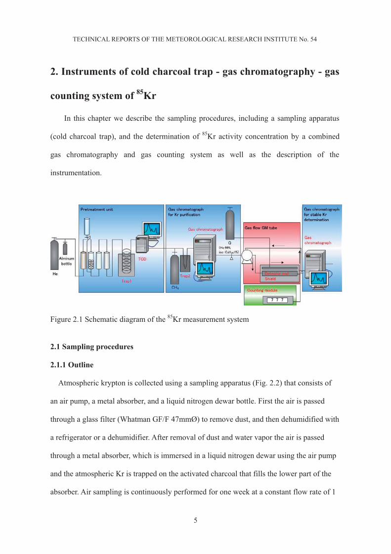
precisely determined with GC 3, the sampling loop of which is also located in the

above-mentioned recirculating loop. Thus the specific activity of 85Kr is obtained from the

activity counting and the stable Kr volume measurements.

Figure 2.9 Schematic flow chart of recirculating loop

2.4.1 Operation of the proportional counter

Figure 2.10 depicts the plateau curve of the center proportional counter that is used for

the 85Kr activity measurement. For the measurement of the plateau curve Kr gas

corresponding to 3% of the recirculating loop volume was introduced and mixed with CH4.

Since the Kr gas produced at present from air already contains 85Kr, pure Kr gas itself is a

good activity source. A counting time of 5 min was applied for each high-voltage value,

giving the counting characteristics of the counter. The signal output began at 3400 V and a

V4(Re.7)

V3( e.6)

V5( e.8)

MV2

SV6(Re.19)

(Re.23)

Flow monitor /Volume monitor

21


plateau was attained between 3600 and 4000 V. Highly stable counting was achieved with

the present proportional counter. Dependent on the counter plateau the high voltage for the

85Kr measurement was set to a value between 3600 and 3800 V to optimize the counting

performance. It should be noted that long use of proportional counters finally result in

disappearance of the plateau. This ageing effect may be caused by the deposition of

carbonaceous material on the surfaces of the detector arising from decomposition of the

measurement gas, CH4.

Figure 2.10 Plateau curve of the center proportional counter

Activity counting (u) gave a good linear response to the stable Kr volume (v) in the

recirculating loop system (in one instance, u=24.84+31.39v, r~0.999, for 0.8-8.0 ml of

stable Kr, n~5). This result indicated that the activity counting was not affected by a trivial

change of gas composition in the proportional counter accompanied by varying Kr content.

22


Table 3 in Igarashi et al., (2001) gave the activity-counting efficiency of the proportional

counter of the MRI system. It was obtained by using the reference Kr gas of which the 85Kr

activity was determined with the BfS system in Freiburg. Thus the MRI and the BfS

systems had a common calibration regarding 85Kr activity measurement. A counting

efficiency of 55 to 60% was achieved with the present system. The data were in good

accordance with the volume ratio of the proportional counter to the whole recirculating

loop suggesting that the active volume of the proportional counter was 85 to 90%.

Currently the proportional counter is shielded by 10 cm thick lead bricks and no other

background reduction procedures have been applied. The background count rate for the

proportional counter is 80 counts min-1. However 85Kr has a relatively high concentration

level of at least 1 Bq m-3, and it is fairly easy to measure 85Kr activity with high precision.

The current detection limit defined by 3.29 times one sigma of background is 0.02 Bq m-3

under the present conditions. Since the detection limit of the stable Kr measurement is of

the order of some tens ppmv at the GC 3, the major factor controlling the detection limit of

this system is the activity measurement rather than stable Kr measurement.

2.4.2 Anti-coincidence counting

We introduced an anti-coincidence technique to reduce the counting background. The

anti-coincidence system consists of a center proportional counter and an outer proportional

counter. The center proportional counter is inserted into the outer proportional counter (No.

49215, LND, USA) for anti-coincidence counting which is operated at a high voltage of

940 V using the counting gas, He 99.05% with 2-methyl-propane 0.95%. The high voltages

for both proportional counters are supplied by a four channel HV power supply unit

(RPH-012, Repic, Japan) and generated signals are amplified by preamplifier (Model

23


142AH, Ortec, USA). The signals from the preamplifier are sent to a discriminator unit

(Model 705, Phillips Scientific, USA). The functions of this unit are to set the threshold

level of the signal height and to convert the signal over the threshold level into digital

signal. The signals are then sent to a gate-delay generator unit (Model 794, Phillips

Scientific, USA). The functions of this unit are to delay the signal from the center

proportional counter and to convert the signal from the outer proportional counter into a

gate signal. Each signal is processed by logic units (Model 756&757, Phillips Scientific,

USA) and an anti-coincidence circuit is built. The signals through the anti-coincidence

circuit are output to a single channel analyzer (RPN-032, Repic, Japan) as counts. The

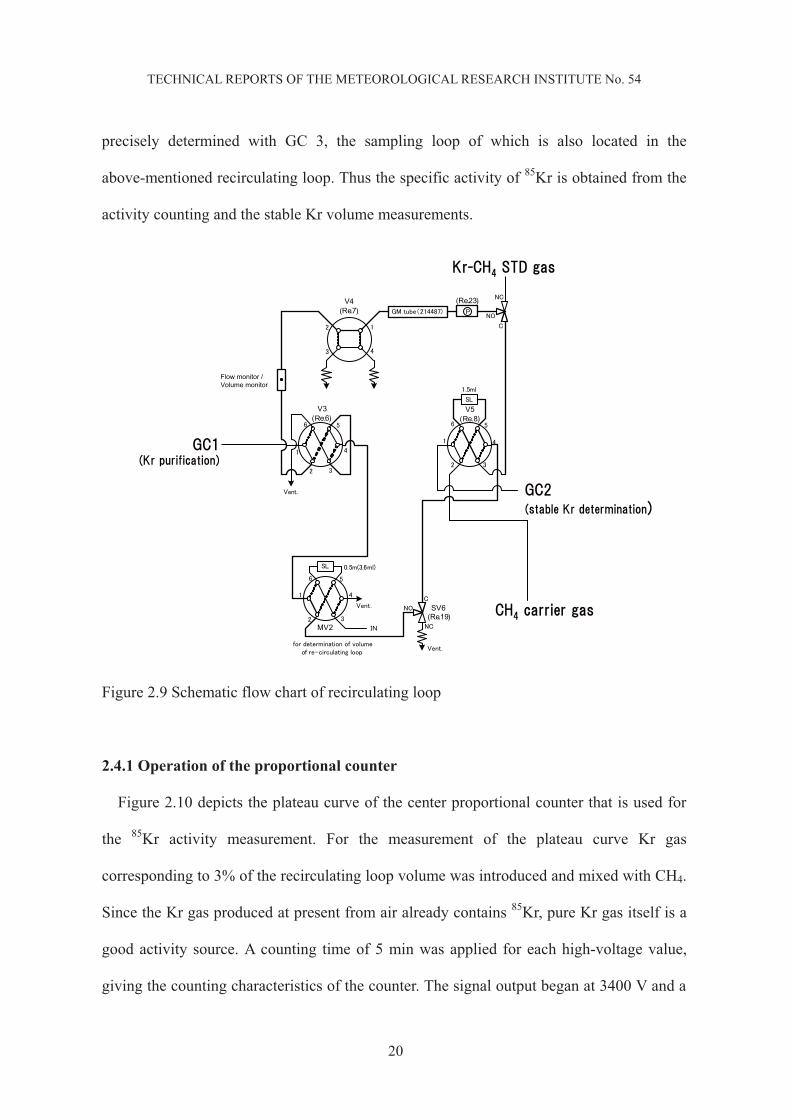
activity-counting unit is presented in Fig. 2.11. Signal cable connections are depicted in Fig.

2.12. In the MRI system, the anti-coincidence technique reduces the background by a

factor of 10 to 8 counts min-1.

24


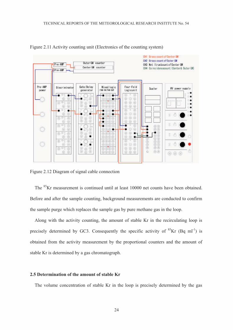
Figure 2.11 Activity counting unit (Electronics of the counting system)

Figure 2.12 Diagram of signal cable connection

The 85Kr measurement is continued until at least 10000 net counts have been obtained.

Before and after the sample counting, background measurements are conducted to confirm

the sample purge which replaces the sample gas by pure methane gas in the loop.

Along with the activity counting, the amount of stable Kr in the recirculating loop is

precisely determined by GC3. Consequently the specific activity of 85Kr (Bq ml-1) is

obtained from the activity measurement by the proportional counters and the amount of

stable Kr is determined by a gas chromatograph.

2.5 Determination of the amount of stable Kr

The volume concentration of stable Kr in the loop is precisely determined by the gas

25


chromatograph (GC2014, Shimadzu, Japan). In this gas chromatograph (GC3) pure He gas

is used as a carrier gas and its main column for separation is packed with MS-5A.

An example of a gas chromatogram is presented in Fig. 2.13. It is important to confirm

that the peaks of krypton and methane are well-separated (not overlapped) in the gas

chromatogram. When the separation of the main column is incomplete, the MS-5A column

should be regenerated or exchanged. The presence of oxygen in the proportional counter

reduces the activity count rate. Confirm that no peaks of air components (O2 and N2) are

present in the gas chromatogram. If air peaks exists in the gas chromatogram, it is

necessary to check the air tightness of each connection and six-ways valve. The Kr gas in

the sample loop in re-circulation loop is subjected to analyze stable krypton concentration.

Figure 2.13 Chromatogram of stable Kr determination

In GC3 the gas in the sample loop (2 ml) is analyzed, after the loop is opened until its

pressure becomes equilibrium with atmospheric pressure. The sample volume determined

with GC3 depends on the temperature and air pressure, Therefore, analytical results

obtained by the GC3 should be corrected to a standard condition for a fixed temperature (0

2.0

0.5

1.0

1.5

00 105 2015 25

Time / min.

Out

put v

olta

ge /

105

V

He gas carrier

Kr

CH4

26


ºC) and air pressure (1 atm), which are monitored in the measurement room. The krypton

volumes are corrected to standard temperature and pressure conditions (STP; 0 ºC, 1 atm).

The Boyle-Charle’s law is applied to the correction of the Kr volume assuming that the Kr

gas behaves as an ideal gas.

Three gravimetric-made standard Kr-CH4 mixed gases are used to calibrate GC3 prior to

and after determine the stable Kr volume in the sample. The stable Kr volume

concentrations in the standard gases using the calibration of the GC3 are determined,

taking into account the Kr amount in the sample gas. The Kr volume concentrations in the

three standard gases used are 0.5, 1 and 3 %.

2.6 Schedule of sample analysis

The time required for a sample analysis is as follows.

Calibration of the GC3 requires three hours before the sample analysis, but this

calibration is performed automatically by a basic program. It takes one hour for the

pre-treatment unit to separate the air components coarsely. It takes 30 minutes to separate

and purify the Kr gas. Two to three hours are needed to measure the activity, depending on

the Kr recovery and its activity level. It takes 30 minutes to determine the concentration of

stable Kr in the sample. Nine hours are needed to carry out all analytical processes,

including in a sample analyis. Therefore, only one sample can be analyzed per day in the

current 85Kr measurement system. The system operation for 85Kr analysis is carried out as

follows.

The pre-treatment unit is turned on just before the sample analysis and turned off after

the sample analysis. However He gas continues to flow at a low flow rate in the

pre-treatment unit to prevent moisture or other redundant components to attach to the

27


pre-treatment tube (Trap1). The GC1 and GC2 use methane gas as a carrier. In

consideration of safety the GC1 and GC2 are turned on just before the sample analysis.

After the sample analysis they are turned off and the carrier gas flow is also stopped. GC3

operates continuously to perform automatic calibration every morning. However, GC3 is

turned off and the carrier gas flow is stopped on the weekend to control the consumption of

He gas.

To ensure the 85Kr measurement system operates normally a standard gas of a known

85Kr activity concentration is analyzed once a week.

This schedule of sample analysis for a week is presented in table 2.1. Three samples can

be analyzed in a week and if the GC3 is operated continuously during a weekend, starting

of the system is unnecessary. Consequently four samples can be analyzed in a week.

Table 2.1 Schedule of sample analysis

If the 85Kr measurement system is shut down for a long time, the schedule is as follows.

For a comparatively short suspension (one week), He gas continues to flow at a rate of

10 ml min-1 through the pre-treatment unit (Trap1). GC3 is turned off and its carrier gas

flow is also stopped. For a long suspension the flow of He gas through the pre-treatment

unit is stopped, the power of this unit is shut down and all the valves are closed. The

Day of the week Operation

Monday System starting

Tuesday Standard gas analysis

Wednesday Sample analysis

Thursday Sample analysis

Friday Sample analysis

28


proportional counter counting unit (e.g., PC and logic units) and other devices, such as the

GC controller (Chromatopac C-R7A, Shimadzu, Japan), are also turned off. In the Kr

enrichment tube (Trap2), a He gas flow continues at a small flow rate. In the proportional

counter CH4 gas continues to flow at a small flow rate or it should be formed a closed loop

to avoid absorption of the air components and moisture to the proportional counter.

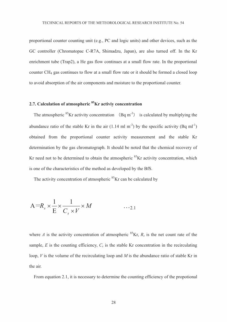
2.7. Calculation of atmospheric 85Kr activiy concentration

The atmospheric 85Kr activity concentration Bq m-3 is calculated by multiplying the

abundance ratio of the stable Kr in the air (1.14 ml m-3) by the specific activity (Bq ml-1)

obtained from the proportional counter activity measurement and the stable Kr

determination by the gas chromatograph. It should be noted that the chemical recovery of

Kr need not to be determined to obtain the atmospheric 85Kr activity concentration, which

is one of the characteristics of the method as developed by the BfS.

The activity concentration of atmospheric 85Kr can be calculated by

MVC

Rs

s1

E1A

where A is the activity concentration of atmospheric 85Kr, Rs is the net count rate of the

sample, E is the counting efficiency, Cs is the stable Kr concentration in the recirculating

loop, V is the volume of the recirculating loop and M is the abundance ratio of stable Kr in

the air.

From equation 2.1, it is necessary to determine the counting efficiency of the propotional

2.1

29


counter in advance to calculate the concentration of the atmospheric 85Kr. There are two

ways to determine the proportional counter counting efficiency. One is to determine the

absolute efficiency for beta particles in the active area by evaluating precisely the

non-active area. The other is to calculate the proportional counter counting efficiency by

using a standard gas with well known 85Kr activity concentration. The first method needs

several kinds of the same type of proportional counters which have different active

volumes with known length and diameter. The counting efficieny of the BfS system was

dertermined applying this method. However this method is not easy, so the latter using the

known concentration standard gas is adopted for the determination of the counting

efficiency of the MRI system.

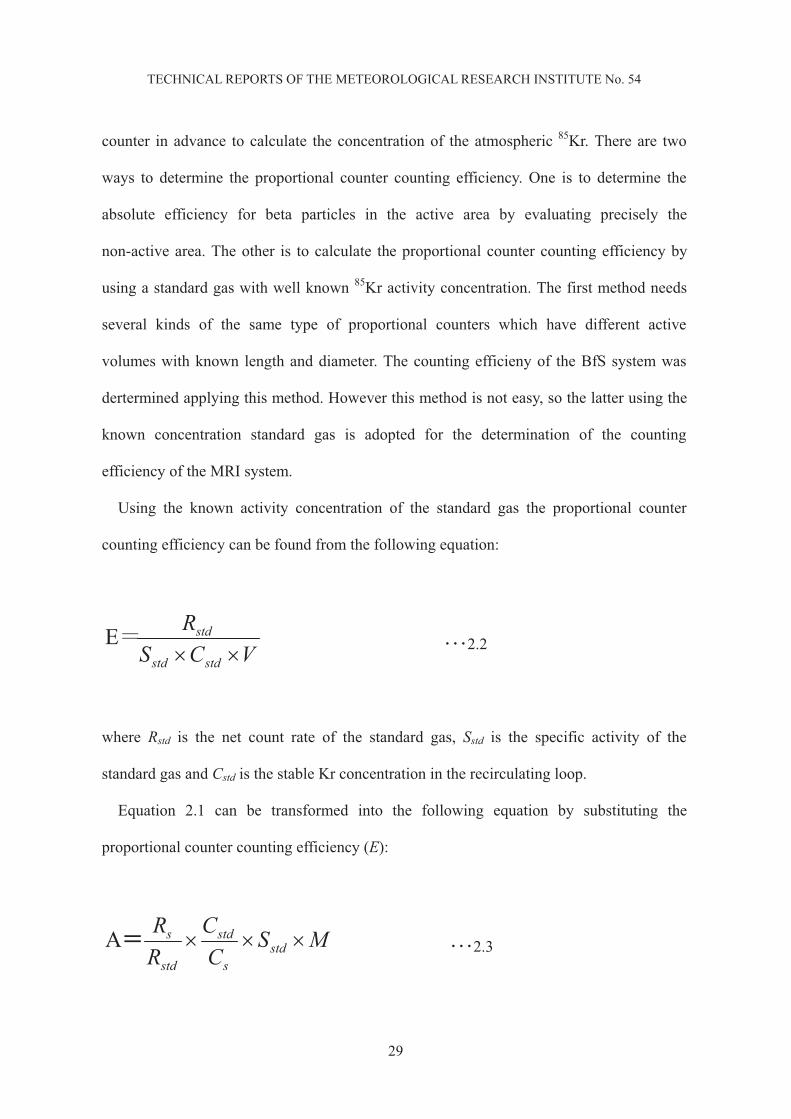
Using the known activity concentration of the standard gas the proportional counter

counting efficiency can be found from the following equation:

VCSR

stdstd

stdE

where Rstd is the net count rate of the standard gas, Sstd is the specific activity of the

standard gas and Cstd is the stable Kr concentration in the recirculating loop.

Equation 2.1 can be transformed into the following equation by substituting the

proportional counter counting efficiency (E):

MSCC

RR

stds

std

std

sA

2.2

2.3

30


2.8 Uncertainty of atmospheric 85Kr activity concentration

We consider two kinds of error terms: accuracy (systematic bias of the data) and

precision (size of the randomness of the data). Accuracy is currently interpreted as

traceability. The traceability of the data is ensured by using the Kr standard gas of which

the 85Kr activity was determined by the BfS. Therefore it is necessary to estimate the

precision of the data separately and it is necessary to estimate the uncertainty involved in

each measurement.

It is necessary to estimate the uncertainty of the proportional counter counting

efficiency and the volume of the recirculationg loop using equation 2.1. However this

equation can be transformed into equation 2.3 by using the mixed standard gas, which has

a known activity concentration of 85Kr. We therefore have to estimate only the uncertainty

involved in the radioactivity measurement, in the stable Kr analysis and of the specific

activity of the mixed standard gas for the determination of the uncertainty of the 85Kr

activity concentration.

a Radioactivity measurement

The uncertainty in the radioactivity measurement is estimated as the result of the

counting error (square root of the count). Since a net counting rate is substituted for a

background counting rate from a gross counting rate, the counting error must be calculated

according to the four rules of arithmetic with error. The uncertainty in the radioactivity

measurement is

31


2

21

212

BB

BBN tt

NNt

N

where N is the uncertainty of the sample ( Ns) and the standard ( Nstd) in the radioactivity

measurement, N is the gross count of the sample (Ns) and the standard (Nstd), NB1 and NB2

are the gross counts of the backgrounds, t is the counting time of the sample (ts) and the

standard (tstd), and tB1 and tB2 are the counting times of the backgrounds.

b Stable Kr analysis

The stable Kr concentration in the recirculationg loop is determined by the working

curve obtained by analyzing the standard gas which has a known concentration of the

stable Kr. Therefore, the concentration of the stable Kr is calculated by the regression line

aEbC 0

where C is the concentration (%) of stable Kr of the sample(Cs) and the standard(Cstd) in

the recirculationg loop. Here, E0 is the accumulated thermal conductivity under standard

conditions (0 ºC, 1atm) of the sample gas and the standard gas, a is the intercept, and b is

the slope of linear regression.

The intercept and slope in this regression curve are included the uncertainty of the Kr

standard gas analysis. This uncertainty spread to the stable Kr concentration in the sample.

When the standard deviations of the intercept and slope are introduced as the uncertainty of

the regression curve, the uncertainty in the stable Kr analysis is

2.4

2.5

32


20

2baC E

where C is the uncertainty of the stable Kr analysis of the sample gas( Cs) and the standard

gas( Cstd), a and b are the standard deviations of the intercept and slope.

The standard deviations of the intercept and slope in the regression curve are defined as

ii

ii

xya xxn

x2

2

/

ii

xyb

xx 2

/

2/12

/ 2

ˆ

n

yyi

ii

xy

where y/x is a statistical value that estimates the accidental error of the direction of a y-axis

in the regression curve and is used for calculating the standard deviations of the intercept

and the slope, xi is the accumulated thermal conductivity in each analysis, x is the

average of the accumulated thermal conductivity, n is the number of the data, yi is the

stable Kr concentration of the standard gas and iy is the stable Kr concentration

calculated by the working curve.

The mixed 85Kr standard gas used to calibrate the 85Kr measurement system was also

2.6

2.7

2.8

2.9

33


used to determine the proportional counter counting efficiency. The specific activity and

the net counting rate of the mixed standard gas are necessary to determine the

concentration of 85Kr. Therefore the 85Kr activity concentration needs not to be determined

the proportional counter counting efficiency and the volume of the recirculationg loop from

equation 2.7.3.

The specific activity determined by the BfS (Sstd ± Sstd) is 0.9781 ± 0.004 Bq ml-1.

We adopt this counting error as the uncertainty of the specific activity.

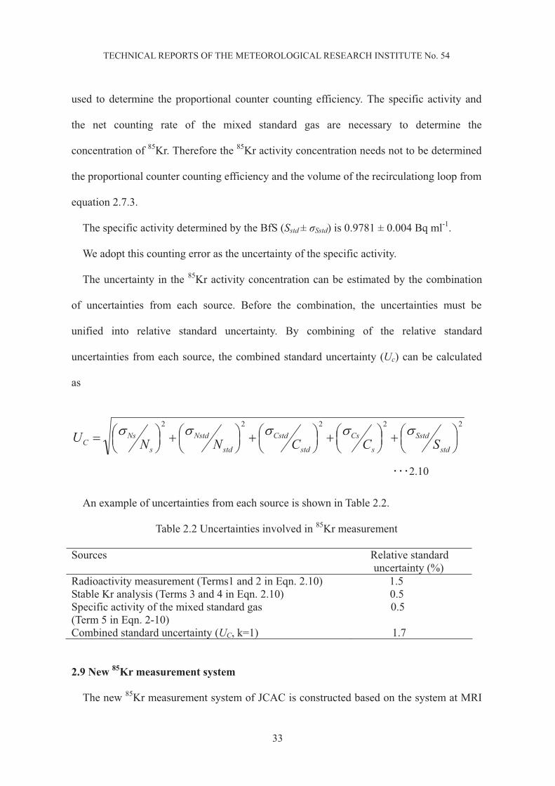
The uncertainty in the 85Kr activity concentration can be estimated by the combination

of uncertainties from each source. Before the combination, the uncertainties must be

unified into relative standard uncertainty. By combining of the relative standard

uncertainties from each source, the combined standard uncertainty (Uc) can be calculated

as

22222

std

Sstd

s

Cs

std

Cstd

std

Nstd

s

NsC SCCNNU

An example of uncertainties from each source is shown in Table 2.2.

Table 2.2 Uncertainties involved in 85Kr measurement

Sources Relative standard uncertainty (%)

Radioactivity measurement (Terms1 and 2 in Eqn. 2.10) 1.5 Stable Kr analysis (Terms 3 and 4 in Eqn. 2.10) 0.5 Specific activity of the mixed standard gas (Term 5 in Eqn. 2-10)

0.5

Combined standard uncertainty (UC, k=1) 1.7

2.9 New 85Kr measurement system

The new 85Kr measurement system of JCAC is constructed based on the system at MRI

2.10

34


along with the technical transfer of the 85Kr monitoring system from MRI to JCAC. This

new system consists of the sampling unit, the pre-treatment unit, the gas chromatographs

for the purification of Kr (GC1) and for the determination of the amount of stable Kr

(GC2) and the proportional counter. Three sampling units have been made in consideration

of the framework of 85Kr monitoring in JCAC.

The 85Kr sampling unit is almost the same as the MRI sampling unit including the metal

absorber. However the instrument for the preliminary removal of moisture has been

modified from a remodeled refrigerator to a thermoelectric dehumidifier (DH-109,

Komatsu Electronics Inc., Japan). The diagram of the sampling unit and the absorber are

presented in Fig. 2.2 and Fig. 2.3, respectively.

The new 85Kr measurement system has some improvements taking into consideration the

framework of JCAC and the convenience of the usage, although the 85Kr measurement

system was also based on the MRI system. The improvements in the system of JCAC are

as follows.

1) The number of the gas chromatographs has been changed from 3 to 2:

In the framework of the environmental radioactivity monitoring at JCAC, the target

noble gaseous radionuclide is 85Kr only, so that the GC2 for purifying Xe was not

considered.

2) In the pre-treatment unit has an additional He gas line for a pure water supply:

The pure water in a water tank can be automatically filled into a water column by

pressurizing He gas.

3) The connection of the cables for the activity measurement has been modified:

The JCAC system uses two proportional counters simultaneously for sample

35


analysis. The delay method of the center proportional counter signal by the gate/delay

generator is changed by passing through the Mixed Logic unit several times. The

signal is delayed by physical processing. The connection of the cables among the units

for the activity measurement of JCAC is illustrated in Fig. 2.12.

36


3. Standard gas for 85Kr measurement

A simulated gas with a composition similar to that of the actual sample gas in the

aluminum bottle (minican) is necessary to calibrate the 85Kr measurement system and to fix

its measurement conditions. In the early stages of development the major gas in the

aluminum bottle was considered to be He and the simulated gas was prepared with the

expected composition. However when the actual sample gas was analyzed, its composition

differed from the expected one. Table 3.1 presents the actual sample gas compositions in

the aluminum bottle along with those of the simulated gas (Takachiho Chemicals, Japan)

based on this determination.

Table 3.1 Gas composition of the sample in the aluminum bottle and the simulated gas Unit: (%)

Sample He Ar N2 O2 Kr CH4 CO2 Xe Total

110-B NA NA 21.5 9.10 0.178 0.192 61.5 NA 92.5

178-B 10.4 NA 17.9 10.5 0.208 0.194 60.3 NA 99.5

179-B 6.89 NA 12.8 16.1 0.234 0.232 63.0 NA 99.3

Average 8.65 NA 17.4 11.9 0.207 0.206 61.6 NA 97.1

Simulated gas B 8.12 0.903 20.9 9.76 1.07 0.949 57.84 0.451 99.55

NA, not analyzed This table is reproduced from Tabble 2 in Igarashi et al., 2001.

The result revealed that a major component of the sample gas in the aluminum bottle is

CO2 rather than He, N2 and O2. This result suggests that CO2 has a high affinity to the

activated charcoal. Therefore the major component in the simulated gas was changed from

He to CO2 (ca. 60%). As a result removal of CO2 became a key point for the activity

37


measurement of 85Kr. The CO2 in the air contains both natural and anthropogenic 14C and

radio carbon interferes with the activity measurement of 85Kr. The alkali-wet column,

which can react more quickly with CO2 in the sample, was therefore devised in the

pre-treatment unit. Water is essential to complete the chemical reaction of CO2 with

alkaline agents. Although water is inadequate for gas chromatographic separation, a wet

column was introduced for effective removal of a large amount of CO2 (more than a few

hundred milliliters).

Usually 4000 ml of the simulated gas was introduced into the system to adjust the whole

85Kr measurement system. Therefore about 2400 ml of CO2, about 800 ml of N2 and about

400 ml of O2 were injected into the pre-treatment unit along with about 40 ml of Kr.

38


4. Atmospheric 85Kr in Japan

4.1 85Kr activity at Tsukuba since 1995

We had observed the weekly average atmospheric 85Kr activity concentrations in ground

level air in Tsukuba during the period from May 1995 to March 2006. Monthly averaged

85Kr activity concentrations are shown in Table 4.1, and weekly atmospheric 85Kr activity

concentration are shown in Table 4.2, respectively. During the period that the nuclear fuel

reprocessing plant at Tokai was in operation (before May 1997 and after June 2000), high

85Kr activity concentrations exceeding 2 Bq m-3 were observed. On the other hand, low

85Kr activity concentrations of less than 1.6 Bq m-3 were observed when operations at the

Tokai plant were suspended. Compared with reprocessing plants in Europe, the magnitude

of the emission at the Tokai plant is less than 10% of those in Europe (United Nations,

2000).

Table 4.1 Monthly averaged atmospheric 85Kr activity concentrations in Tsukuba Unit: Bq m-3

1995 1996 1997 1998 1999 2000 2001 2002 2003 2004 2005 2006Jan 1.26 1.26 1.3 1.37 1.35 1.36 1.46 1.45 1.89 1.50 1.50 Feb 1.24 3.34 1.31 1.36 1.37 1.34 1.47 1.43 1.94 2.43 3.94 Mar 1.23 1.29 1.29 1.37 1.36 1.92 1.55 1.44 1.78 4.80 1.52 Apr 2.44 1.27 1.27 1.37 1.38 3.13 3.88 1.45 1.99 2.82 May 6.88 4.35 1.31 1.29 1.36 1.32 2.48 4.86 1.49 2.55 2.76 Jun 2.11 2.29 1.26 1.25 1.32 1.33 2.85 3.50 1.44 1.45 1.45 Jul 1.08 1.16 1.23 1.21 1.25 2.02 1.29 1.30 1.41 1.40 1.44 Aug 1.06 1.16 1.19 1.21 1.24 1.25 1.33 1.32 1.36 1.43 1.40 Sep 5.3 1.99 1.23 1.22 1.3 1.3 1.39 1.37 2.40 1.45 1.40 Oct 4.29 5.03 1.27 1.32 1.39 1.37 3.18 2.09 3.55 4.92 2.80 Nov 1.76 2.2 1.33 1.35 1.37 1.46 1.85 1.69 2.54 2.08 2.41 Dec 1.33 1.23 1.36 1.4 1.41 1.39 1.51 1.50 1.47 1.54 1.53 note: Monthly averaged atmospheric 85Kr activity concentrations during the period from 1995 to 2001 are cited from Hirota et al., 2004.

39


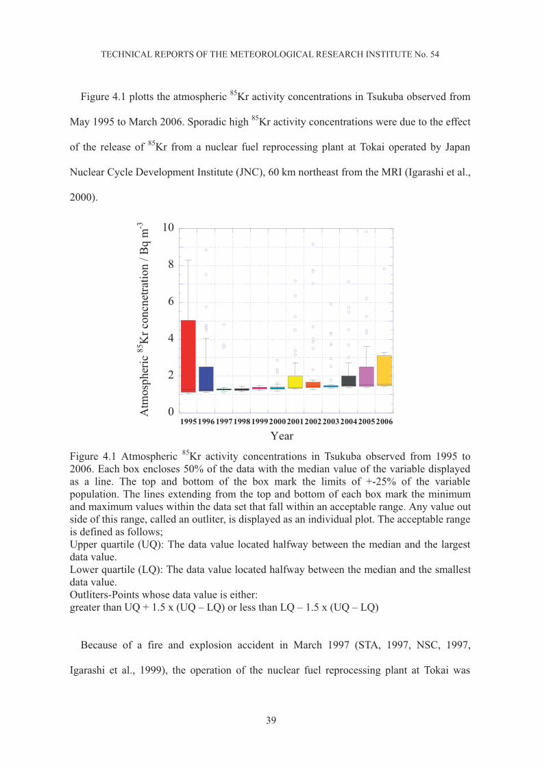
Figure 4.1 plotts the atmospheric 85Kr activity concentrations in Tsukuba observed from

May 1995 to March 2006. Sporadic high 85Kr activity concentrations were due to the effect

of the release of 85Kr from a nuclear fuel reprocessing plant at Tokai operated by Japan

Nuclear Cycle Development Institute (JNC), 60 km northeast from the MRI (Igarashi et al.,

2000).

0

2

4

6

8

10

199519961997199819992000200120022003200420052006

Atm

osph

eric

85K

r con

cnet

ratio

n / B

q m

-3

Year

Figure 4.1 Atmospheric 85Kr activity concentrations in Tsukuba observed from 1995 to 2006. Each box encloses 50% of the data with the median value of the variable displayed as a line. The top and bottom of the box mark the limits of +-25% of the variable population. The lines extending from the top and bottom of each box mark the minimum and maximum values within the data set that fall within an acceptable range. Any value out side of this range, called an outliter, is displayed as an individual plot. The acceptable range is defined as follows; Upper quartile (UQ): The data value located halfway between the median and the largest data value. Lower quartile (LQ): The data value located halfway between the median and the smallest data value. Outliters-Points whose data value is either: greater than UQ + 1.5 x (UQ – LQ) or less than LQ – 1.5 x (UQ – LQ)

Because of a fire and explosion accident in March 1997 (STA, 1997, NSC, 1997,

Igarashi et al., 1999), the operation of the nuclear fuel reprocessing plant at Tokai was

40


discontinued until the summer of 2000. During this period, no sporadic high 85Kr activity

concentrations in surface air were observed in Tsukuba. Experimental operation of the

nuclear fuel reprocessing plant in Tokai was conducted in the summer of 2000, and its

routine operation was restarted in the spring of 2001. Since that time, sporadic increases of

atmospheric 85Kr activity concentrations have occurred again in Tsukuba. For the public’s

radiation protection, it is important to know the background level of the atmospheric 85Kr

activity concentrations in Japan. For the background level of atmospheric 85Kr activity

concentrations in Tsukuba, data affected by 85Kr release from the Tokai plant should be

removed. Since the effect of 85Kr release from the Tokai plant toto the atmosphere in

Tsukuba depends on wind direction, wind speed, and daily 85Kr release rate from the Tokai

plant (Igarashi et al., 2000), all of the observed data in the sampling period including the

days when the Tokai plant has been in operation were removed regardless of the 85Kr

activity concentration measured at MRI. The background data obtained are plotted in Fig.

4.2

The background atmospheric 85Kr activity concentrations in Tsukuba have been

increasing, accompanied by seasonal variations throughout our study period. Hirota et al.

(2004) had showed that annual growth rate from 1996 to 2001 in Tsukuba was calculated

to be 0.03 Bq m-3 yr-1. This rate was at the same level as a previous estimate for the period

of 1996 - 1998 (Igarashi et al. 2000). During the period from 1995 to 2006, the linear

regression of atmospheric 85Kr activity concentration also showed similar increasing

rate of 0.03 Bq m-3 yr-1. However, it must be noted that the growth rate varied annually,

especially atmospheric 85Kr activity concentration are almost constant since 2004. The

mean annual growth rate of 0.03 Bq m-3 yr-1is independently observed at all other stations

of the global BfS noble gas network. The background values measured at the sites on the

41


Northern Hemisphere of the global BfS network are in good agreement with the one

measured during winter time at MRI in Tsukuba. Pollard et al. (1997) reported the

atmospheric 85Kr activity concentrations at Clonskeagh, Dublin, Ireland, between 1994 and

1996. Excluding the data exceeding 2.5 Bq m-3 as outliers, the mean annual 85Kr activity

concentration was 1.12 Bq m-3 during 1994 and 1.30 Bq m-3 during 1996, and an increasing

trend of approximately 0.1 Bq m-3 yr-1 was observed which is app. a factor of 3 higher than

the ones measured at other sites in Europe and Japan. The atmospheric 85Kr activity

concentrations in Dublin from 1994 to1996 were in agreement with those observed in

winter at the MRI, Tsukuba.

0.5

1.0

1.5

2.0

1996 1998 2000 2002 2004 2006

Atm

osph

eric

85K

r con

cnet

ratio

n / B

q m

-3

YearFigure 4.2 Atmospheric background 85Kr activity concentrations in Tsukuba

The background atmospheric 85Kr activity concentrations in Japan indicated a clear

seasonal variation which is characterized as low in summer and high in winter. To explain

this pattern of seasonal variation Hirota et al., (2004) had carried out the backward

42


trajectory analysis by using 85Kr data observed in Tsukuba in 1999. They used Global

Analysis Data (GANAL) compiled by the Japan Meteorological Agency for wind data

analysis. A total of 240 hours backward data (starting at an altitude of 1,500 m, about 850

hPa; 00 UTC) was calculated every 5 days. Figure 4.3(a) illustrates typical examples of the

backward trajectory in winter and Figure 4.3(b) depicts those, respectively.

Figure 4.3 Typical charts of backward trajectory in winter and in summer. The point for each category is shown on the globe. (a) the chart for 10 days from January 5, 1999. (b) the chart for 10 days from August 3, 1999. (Hirota et al, 2004, figure 5)

In their analysis the origin of air mass transported to Tsukuba was estimated. The

origins were grouped by four categories centering on Tsukuba, and they introduced the

“Trajectory Index” of air masses to reflect the relative distribution of the global

atmospheric 85Kr activity concentrations. This index is defined as a mean of the points

during the sampling period, in which the point on each day is assigned from the category of

the trajectory (Figure 4.3). Since most of the nuclear fuel reprocessing plants are located in

Europe, it is considered that the area classified as category 1 shows the highest

concentrations of 85Kr, i.e., the highest point. The areas classified as categories 3 and 4

43


show the lowest concentrations of 85Kr, i.e., the lowest point. This classification reflects a

latitudinal gradient of the atmospheric 85Kr activity concentrations, high in the northern air

mass and low in the southern air mass, which is in agreement with the observations

reported by Weiss et al. (1992). We examined the correlation between the “Trajectory

Index” and the observed atmospheric 85Kr activity concentrations and found a good

correlation between them (correlation factor 0.67) was found. Using a linear regression

obtained from this correlation, we estimated 85Kr activity concentrations in Tsukuba from

the indexes. Figure 4.4 shows the comparison between the observed 85Kr activity

concentrations and the estimated ones from the indexes in Tsukuba. The result suggests

that the seasonal variation of the atmospheric 85Kr activity concentrations in Tsukuba,

Japan, is mainly controlled by the transport of the air masses with different origins and that

the high concentrations from October to May are attributable to the transport of the

continental air mass directly affected by the European sources.

Figure 4.4 Comparison between the observed 85Kr activity concentrations and the estimated ones from the “Trajectory Indexes” in Tsukuba in 1999. (Hirota et al., 2004 Figure 6)

44


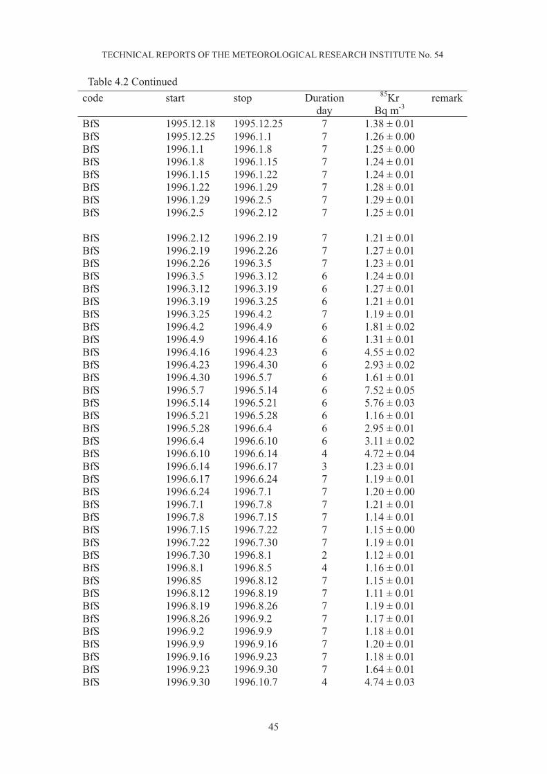
Table 4.2 Weekly atmospheric 85Kr activity concentration at Tsukuba during the period from May 1995 to March 2006.

code start stop Duration day

85KrBq m-3

remark

BfS 1995.5.1 1995.5.8 7 7.67 ± 0.06 BfS 1995.5.1 1995.5.8 7 7.78 ± 0.02 BfS 1995.5.1 1995.5.8 7 7.72 ± 0.23 * BfS 1995.5.8 1995.5.15 7 14.20 ± 0.06 BfS 1995.5.15 1995.5.22 7 3.28 ± 0.03 BfS 1995.5.22 1995.5.29 7 6.02 ± 0.03 BfS 1995.5.29 1995.6.5 6 3.16 ± 0.03 BfS 1995.6.5 1995.6.12 7 5.03 ± 0.05 BfS 1995.6.5 1995.6.12 7 5.05 ± 0.05 BfS 1995.6.5 1995.6.12 7 4.98 ± 0.03 BfS 1995.6.5 1995.6.12 7 5.02 ± 0.15 * BfS 1995.6.12 1995.6.19 6 1.19 ± 0.04 BfS 1995.6.12 1995.6.19 6 1.19 ± 0.01 BfS 1995.6.12 1995.6.19 6 1.19 ± 0.01 * BfS 1995.6.19 1995.6.26 7 1.14 ± 0.01 BfS 1995.6.26 1995.7.3 7 1.11 ± 0.01 1995.7.3 7 N.A ** BfS 1995.7.10 1995.7.14 4 1.10 ± 0.01 BfS 1995.7.14 1995.7.18 3 1.12 ± 0.01 BfS 1995.7.18 1995.7.28 6 1.08 ± 0.01 1995.7.24 4 ** BfS 1995.7.28 1995.8.1 3 1.04 ± 0.01 BfS 1995.8.1 1995.8.7 6 1.03 ± 0.01 BfS 1995.8.7 1995.8.14 5 1.08 ± 0.01 BfS 1995.8.14 1995.8.21 7 1.06 ± 0.01 BfS 1995.8.21 1995.8.28 4 1.04 ± 0.01 BfS 1995.8.28 1995.9.4 7 1.08 ± 0.01 BfS 1995.9.4 1995.9.11 7 1.16 ± 0.01 BfS 1995.9.11 1995.9.18 7 1.15 ± 0.00 1995.9.18 7 N.A ** BfS 1995.9.25 1995.9.25 5 13.60 ± 0.10 BfS 1995.9.25 1995.10.9 5 3.60 ± 0.05 BfS 1995.10.9 1995.10.16 7 6.39 ± 0.03 BfS 1995.10.16 1995.10.23 4 8.30 ± 0.03 BfS 1995.10.23 1995.10.30 7 1.21 ± 0.01 BfS 1995.10.30 1995.11.6 7 1.26 ± 0.01 BfS 1995.11.6 1995.11.13 7 1.22 ± 0.01 BfS 1995.11.13 1995.11.20 7 3.11 ± 0.02 BfS 1995.11.20 1995.11.27 7 1.41 ± 0.01 BfS 1995.11.27 1995.12.4 7 1.28 ± 0.01 BfS 1995.12.4 1995.12.11 7 1.27 ± 0.01 BfS 1995.12.11 1995.12.18 7 1.42 ± 0.00

45



85KrBq m-3

remark

BfS 1995.12.18 1995.12.25 7 1.38 ± 0.01 BfS 1995.12.25 1996.1.1 7 1.26 ± 0.00 BfS 1996.1.1 1996.1.8 7 1.25 ± 0.00 BfS 1996.1.8 1996.1.15 7 1.24 ± 0.01 BfS 1996.1.15 1996.1.22 7 1.24 ± 0.01 BfS 1996.1.22 1996.1.29 7 1.28 ± 0.01 BfS 1996.1.29 1996.2.5 7 1.29 ± 0.01 BfS 1996.2.5 1996.2.12 7 1.25 ± 0.01 BfS 1996.2.12 1996.2.19 7 1.21 ± 0.01 BfS 1996.2.19 1996.2.26 7 1.27 ± 0.01 BfS 1996.2.26 1996.3.5 7 1.23 ± 0.01 BfS 1996.3.5 1996.3.12 6 1.24 ± 0.01 BfS 1996.3.12 1996.3.19 6 1.27 ± 0.01 BfS 1996.3.19 1996.3.25 6 1.21 ± 0.01 BfS 1996.3.25 1996.4.2 7 1.19 ± 0.01 BfS 1996.4.2 1996.4.9 6 1.81 ± 0.02 BfS 1996.4.9 1996.4.16 6 1.31 ± 0.01 BfS 1996.4.16 1996.4.23 6 4.55 ± 0.02 BfS 1996.4.23 1996.4.30 6 2.93 ± 0.02 BfS 1996.4.30 1996.5.7 6 1.61 ± 0.01 BfS 1996.5.7 1996.5.14 6 7.52 ± 0.05 BfS 1996.5.14 1996.5.21 6 5.76 ± 0.03 BfS 1996.5.21 1996.5.28 6 1.16 ± 0.01 BfS 1996.5.28 1996.6.4 6 2.95 ± 0.01 BfS 1996.6.4 1996.6.10 6 3.11 ± 0.02 BfS 1996.6.10 1996.6.14 4 4.72 ± 0.04 BfS 1996.6.14 1996.6.17 3 1.23 ± 0.01 BfS 1996.6.17 1996.6.24 7 1.19 ± 0.01 BfS 1996.6.24 1996.7.1 7 1.20 ± 0.00 BfS 1996.7.1 1996.7.8 7 1.21 ± 0.01 BfS 1996.7.8 1996.7.15 7 1.14 ± 0.01 BfS 1996.7.15 1996.7.22 7 1.15 ± 0.00 BfS 1996.7.22 1996.7.30 7 1.19 ± 0.01 BfS 1996.7.30 1996.8.1 2 1.12 ± 0.01 BfS 1996.8.1 1996.8.5 4 1.16 ± 0.01 BfS 1996.85 1996.8.12 7 1.15 ± 0.01 BfS 1996.8.12 1996.8.19 7 1.11 ± 0.01 BfS 1996.8.19 1996.8.26 7 1.19 ± 0.01 BfS 1996.8.26 1996.9.2 7 1.17 ± 0.01 BfS 1996.9.2 1996.9.9 7 1.18 ± 0.01 BfS 1996.9.9 1996.9.16 7 1.20 ± 0.01 BfS 1996.9.16 1996.9.23 7 1.18 ± 0.01 BfS 1996.9.23 1996.9.30 7 1.64 ± 0.01 BfS 1996.9.30 1996.10.7 4 4.74 ± 0.03

Table 4.2 Continued

46



85KrBq m-3

remark

BfS 1996.10.7 1996.10.15 7 8.85 ± 0.05 BfS 1996.10.15 1996.10.21 3 4.50 ± 0.04 BfS 1996.10.21 1996.10.28 7 2.72 ± 0.01 BfS 1996.10.28 1996.11.5 7 4.05 ± 0.02 BfS 1996.11.5 1996.11.11 6 3.09 ± 0.02 BfS 1996.11.11 1996.11.18 7 1.65 ± 0.04 BfS 1996.11.18 1996.11.25 7 2.50 ± 0.01 BfS 1996.11.25 1996.12.2 7 1.56 ± 0.01 BfS 1996.12.2 1996.12.9 7 1.26 ± 0.01 BfS 1996.12.9 1996.12.16 7 1.25 ± 0.01 BfS 1996.12.16 1996.12.23 7 1.23 ± 0.01 BfS 1996.12.23 1996.12.25 2 1.22 ± 0.02 BfS 1996.12.25 1997.1.6 2 1.22 ± 0.00 BfS 1997.1.6 1997.1.13 7 1.24 ± 0.01 BfS 1997.1.13 1997.1.20 7 1.21 ± 0.01 BfS 1997.1.20 1997.1.27 7 1.33 ± 0.01 BfS 1997.1.27 1997.2.3 7 1.28 ± 0.01 BfS 1997.2.3 1997.2.10 7 4.82 ± 0.02 BfS 1997.2.10 1997.2.17 7 3.69 ± 0.02 BfS 1997.2.17 1997.2.24 4 1.29 ± 0.01 BfS 1997.2.24 1997.3.3 7 3.56 ± 0.04 7 N.A 7 N.A 5 N.A BfS 1997.3.15 1997.3.17 2 1.30 ± 0.01 BfS 1997.3.17 1997.3.24 7 1.30 ± 0.01 BfS 1997.3.24 1997.3.31 7 1.30 ± 0.01 BfS 1997.3.31 1997.4.7 7 1.26 ± 0.01 BfS 1997.4.7 1997.4.14 7 1.25 ± 0.01 BfS 1997.4.14 1997.4.21 7 1.29 ± 0.01 BfS 1997.4.21 1997.4.28 7 1.26 ± 0.01 BfS 1997.4.28 1997.5.5 7 1.29 ± 0.01 BfS 1997.5.5 1997.5.12 7 1.28 ± 0.01 BfS 1997.5.12 1997.5.19 7 1.26 ± 0.01 BfS 1997.5.19 1997.5.26 7 1.35 ± 0.01 BfS 1997.5.26 1997.6.3 7 1.33 ± 0.01 BfS 1997.6.3 1997.6.9 6 1.30 ± 0.01 BfS 1997.6.9 1997.6.16 7 1.29 ± 0.01 BfS 1997.6.16 1997.6.23 7 1.22 ± 0.01 BfS 1997.6.23 1997.6.30 7 1.28 ± 0.01 BfS 1997.6.30 1997.7.7 7 1.19 ± 0.01 BfS 1997.7.7 1997.7.14 7 1.21 ± 0.01 BfS 1997.7.14 1997.7.21 7 1.26 ± 0.01 BfS 1997.7.21 1997.7.28 7 1.28 ± 0.01 BfS 1997.7.28 1997.8.4 7 1.19 ± 0.01

Table 4.2 Continued

47



85KrBq m-3

remark

BfS 1997.8.4 1997.8.11 4 1.13 ± 0.01 BfS 1997.8.11 1997.8.18 7 1.18 ± 0.01 BfS 1997.8.18 1997.8.25 7 1.21 ± 0.01 BfS 1997.8.25 1997.9.1 7 1.24 ± 0.01 BfS 1997.9.1 1997.9.8 7 1.16 ± 0.01 BfS 1997.9.8 1997.9.16 4 1.21 ± 0.01 BfS 1997.9.16 1997.9.22 6 1.25 ± 0.01 BfS 1997.9.22 1997.9.29 7 1.30 ± 0.02 BfS 1997.9.29 1997.10.6 4 1.25 ± 0.01 BfS 1997.10.6 1997.10.13 3 1.25 ± 0.01 BfS 1997.10.13 1997.10.20 4 1.31 ± 0.01 BfS 1997.10.20 1997.10.27 7 1.26 ± 0.01 BfS 1997.10.27 1997.11.4 6 1.28 ± 0.01 BfS 1997.11.4 1997.11.10 6 1.31 ± 0.01 BfS 1997.11.10 1997.11.17 7 1.31 ± 0.01 BfS 1997.11.17 1997.11.25 4 1.34 ± 0.01 BfS 1997.11.25 1997.12.1 6 1.34 ± 0.01 BfS 1997.12.1 1997.12.8 7 1.39 ± 0.01 BfS 1997.12.8 1997.12.15 7 1.34 ± 0.01 BfS 1997.12.15 1997.12.22 7 1.35 ± 0.01 BfS 1997.12.22 1998.1.5 7 1.36 ± 0.01 BfS 1998.1.5 1998.1.13 6 1.32 ± 0.01 BfS 1998.1.13 1998.1.19 6 1.31 ± 0.01 BfS 1998.1.19 1998.1.26 7 1.32 ± 0.01 BfS 1998.1.26 1998.2.2 7 1.34 ± 0.01 BfS 1998.2.2 1998.2.9 7 1.33 ± 0.01 BfS 1998.2.9 1998.2.16 7 1.30 ± 0.01 BfS 1998.2.16 1998.2.23 7 1.34 ± 0.01 BfS 1998.2.23 1998.3.2 7 1.28 ± 0.01 BfS 1998.3.2 1998.3.9 7 1.29 ± 0.01 BfS 1998.3.9 1998.3.16 7 1.30 ± 0.01 BfS 1998.3.16 1998.3.23 7 1.33 ± 0.01 BfS 1998.3.23 1998.3.30 7 1.28 ± 0.01 BfS 1998.3.30 1998.4.6 7 1.28 ± 0.01 BfS 1998.4.6 1998.4.13 7 1.26 ± 0.01 BfS 1998.4.13 1998.4.20 7 1.28 ± 0.01 BfS 1998.4.20 1998.4.27 7 1.26 ± 0.01 BfS 1998.4.27 1998.5.6 5 1.29 ± 0.01 BfS 1998.5.6 1998.5.11 5 1.27 ± 0.01 BfS 1998.5.11 1998.5.14 7 1.35 ± 0.01 BfS 1998.5.14 1998.5.18 5 1.23 ± 0.01 BfS 1998.5.18 1998.5.25 7 1.25 ± 0.01 BfS 1998.5.25 1998.6.1 7 1.29 ± 0.01 BfS 1998.6.1 1998.6.2 7 1.26 ± 0.01 BfS 1998.6.2 1998.6.8 3 1.32 ± 0.01

Table 4.2 Continued

48



85KrBq m-3

remark

BfS 1998.6.8 1998.615 7 1.27 ±0.01 BfS 1998.6.15 1998.6.22 7 1.32 ±0.01 BfS 1998.6.22 1998.6.29 7 1.21 ±0.01 BfS 1998.6.29 1998.7.6 7 1.20 ±0.01 7 N.A BfS 1998.7.13 1998.7.21 4 1.27 ± 0.00 BfS 1998.7.21 1998.7.29 8 1.17 ± 0.01 BfS 1998.7.29 1998.8.3 5 1.18 ± 0.01 BfS 1998.8.3 1998.8.10 7 1.23 ± 0.01 BfS 1998.8.10 1998.8.17 7 1.23 ± 0.01 BfS 1998.8.17 1998.8.24 7 1.23 ± 0.01 BfS 1998.8.24 1998.8.31 7 1.16 ± 0.01 BfS 1998.8.31 1998.9.7 7 1.21 ± 0.01 BfS 1998.9.7 1998.9.14 7 1.29 ± 0.01 BfS 1998.9.14 1998.9.21 7 1.19 ± 0.01 BfS 1998.9.21 1998.9.28 7 1.18 ± 0.01 BfS 1998.9.28 1998.10.5 7 1.25 ± 0.01 BfS 1998.10.5 1998.10.12 5 1.34 ± 0.01 BfS 1998.10.12 1998.10.19 7 1.29 ± 0.01 BfS 1998.10.19 1998.10.26 4 1.31 ± 0.01 BfS 1998.10.26 1998.11.3 7 1.32 ± 0.01 7 N.A BfS 1998.11.9 1998.11.16 7 1.37 ± 0.01 BfS 1998.11.16 1998.11.23 7 1.32 ± 0.01 BfS 1998.11.23 1998.11.30 7 1.36 ± 0.01 BfS 1998.11.30 1998.12.7 7 1.36 ± 0.01 BfS 1998.12.7 1998.12.14 7 1.35 ± 0.01 BfS 1998.12.14 1998.12.21 7 1.36 ± 0.01 BfS 1998.12.21 1998.12.28 7 1.44 ± 0.01 BfS 1998.12.28 1999.1.4 7 1.45 ± 0.00 BfS 1999.1.4 1999.1.11 7 1.45 ± 0.01 BfS 1999.1.11 1999.1.18 7 1.41 ± 0.01 BfS 1999.1.18 1999.1.25 7 1.30 ± 0.01 BfS 1999.1.25 1999.2.1 7 1.32 ± 0.01 BfS 1999.2.1 1999.2.8 7 1.32 ± 0.01 BfS 1999.2.8 1999.2.15 7 1.34 ± 0.01 BfS 1999.2.15 1999.2.22 7 1.37 ± 0.01 BfS 1999.2.22 1999.3.1 7 1.42 ± 0.01 BfS 1999.3.1 1999.3.8 7 1.34 ± 0.01 BfS 1999.3.8 1999.3.15 7 1.40 ± 0.01 BfS 1999.3.15 1999.3.23 5 1.33 ± 0.01 BfS 1999.3.23 1999.3.29 6 1.37 ± 0.01 BfS 1999.3.29 1999.4.5 7 1.41 ± 0.01 BfS 1999.4.5 1999.4.12 7 1.36 ± 0.01 BfS 1999.4.12 1999.4.19 7 1.36 ± 0.01

Table 4.2 Continued

49



85KrBq m-3

remark

BfS 1999.4.19 1999.4.26 7 1.36 ± 0.01 BfS 1999.4.26 1999.5.3 7 1.40 ± 0.01 BfS 1999.5.3 1999.5.10 7 1.41 ± 0.01 BfS 1999.5.10 1999.5.17 7 1.39 ± 0.01 BfS 1999.5.17 1999.5.24 7 1.33 ± 0.02 BfS 1999.5.24 1999.5.31 7 1.31 ± 0.01 BfS 1999.5.31 1999.6.7 7 1.35 ± 0.01 BfS 1999.6.7 1999.6.14 7 1.34 ± 0.01 BfS 1999.6.14 1999.6.21 7 1.31 ± 0.01 BfS 1999.6.21 1999.6.28 7 1.36 ± 0.01 BfS 1999.6.28 1999.7.5 7 1.27 ± 0.01 BfS 1999.7.5 1999.7.12 7 1.31 ± 0.01 BfS 1999.7.12 1999.7.19 7 1.22 ± 0.01 BfS 1999.7.19 1999.7.26 7 1.24 ± 0.01 BfS 1999.7.26 1999.8.2 7 1.24 ± 0.01 BfS 1999.8.2 1999.8.9 7 1.23 ± 0.01 BfS 1999.8.9 1999.8.16 7 1.22 ± 0.01 7 N.A BfS 1999.8.23 1999.8.30 7 1.26 ± 0.01 BfS 1999.8.30 1999.9.6 7 1.26 ± 0.01 BfS 1999.9.6 1999.9.13 7 1.28 ± 0.00 BfS 1999.9.13 1999.9.20 7 1.24 ± 0.01 BfS 1999.9.20 1999.9.27 7 1.30 ± 0.02 BfS 1999.9.27 1999.9.30 3 1.33 ± 0.01 BfS 1999.9.30 1999.10.1 1 1.38 ± 0.07 BfS 1999.10.1 1999.10.2 1 1.36 ± 0.01 BfS 1999.10.2 1999.10.4 2 1.37 ± 0.01 BfS 1999.10.4 1999.10.12 4 1.47 ± 0.01 BfS 1999.10.12 1999.10.18 6 1.35 ± 0.01 BfS 1999.10.18 1999.10.25 4 1.38 ± 0.01 BfS 1999.10.25 1999.11.1 7 1.39 ± 0.01 BfS 1999.11.1 1999.11.8 7 1.36 ± 0.01 BfS 1999.11.8 1999.11.15 7 1.44 ± 0.01 BfS 1999.11.15 1999.11.22 7 1.38 ± 0.01 BfS 1999.11.22 1999.11.29 7 1.33 ± 0.01 BfS 1999.11.29 1999.12.6 7 1.37 ± 0.03 BfS 1999.12.6 1999.12.13 7 1.44 ± 0.00 BfS 1999.12.13 1999.12.20 7 1.42 ± 0.01 BfS 1999.12.20 1999.12.27 7 1.39 ± 0.01 BfS 1999.12.27 2000.1.3 7 1.37 ± 0.02 BfS 2000.1.3 2000.1.10 7 1.33 ± 0.01 BfS 2000.1.10 2000.1.17 7 1.40 ± 0.01 BfS 2000.1.17 2000.1.24 7 1.39 ± 0.01 BfS 2000.1.24 2000.1.31 7 1.33 ± 0.01 BfS 2000.1.31 2000.2.7 7 1.32 ± 0.01

Table 4.2 Continued

50



85KrBq m-3

remark

BfS 2000.2.7 2000.2.14 7 1.33 ± 0.01 BfS 2000.2.14 2000.2.21 7 1.35 ± 0.01 BfS 2000.2.21 2000.2.28 4 1.50 ± 0.01 BfS 2000.2.28 2000.3.6 7 1.33 ± 0.01 BfS 2000.3.6 2000.3.13 7 1.39 ± 0.05 BfS 2000.3.13 2000.3.21 4 1.34 ± 0.01 BfS 2000.3.21 2000.3.27 6 1.36 ± 0.03 BfS 2000.3.27 2000.3.31 4 1.36 ± 0.01 10 N.A MRI_non_anti 2000.4.10 2000.4.17 7 1.39 ± 0.14 MRI_non_anti 2000.4.17 2000.4.24 7 1.33 ± 0.13 MRI_non_anti 2000.4.24 2000.5.1 7 1.38 ± 0.14 MRI_non_anti 7 N.A MRI_non_anti 2000.5.8 2000.5.15 7 1.34 ± 0.08 MRI_non_anti 2000.5.15 2000.5.22 7 1.34 ± 0.12 MRI_non_anti 2000.5.22 2000.5.29 7 1.24 ± 0.06 MRI_non_anti 2000.5.29 2000.6.5 7 1.27 ± 0.06 MRI_non_anti 2000.6.5 2000.6.12 7 1.27 ± 0.06 MRI_non_anti 2000.6.12 2000.6.19 7 1.27 ± 0.18 MRI_non_anti 2000.6.19 2000.6.26 7 1.38 ± 0.09 MRI_non_anti 2000.6.26 2000.7.3 7 1.26 ± 0.05 MRI_non_anti 2000.7.3 2000.7.10 7 2.35 ± 0.09 MRI_non_anti 2000.7.10 2000.7.17 7 2.19 ± 0.08 MRI_non_anti 2000.7.17 2000.7.24 7 2.85 ± 0.12 MRI_non_anti 2000.7.24 2000.7.31 7 1.24 ± 0.04 MRI_non_anti 2000.7.31 2000.8.7 7 1.19 ± 0.05 MRI_non_anti 2000.8.7 2000.8.14 7 1.20 ± 0.06 MRI_non_anti 2000.8.14 2000.8.21 7 1.29 ± 0.04 MRI_non_anti 2000.8.21 2000.8.28 7 1.25 ± 0.04 MRI_non_anti 2000.8.28 2000.9.4 7 1.27 ± 0.04 MRI_non_anti 2000.9.4 2000.9.11 7 1.23 ± 0.04 MRI_non_anti 2000.9.11 2000.9.18 7 1.29 ± 0.04 MRI_non_anti 2000.9.18 2000.9.25 7 1.38 ± 0.06 MRI_non_anti 2000.9.25 2000.10.2 7 1.33 ± 0.04 MRI_non_anti 2000.10.2 2000.10.10 8 1.56 ± 0.05 MRI_non_anti 2000.10.10 2000.10.16 6 1.37 ± 0.06 MRI_non_anti 2000.10.16 2000.10.23 7 1.39 ± 0.04 MRI_non_anti 2000.10.23 2000.10.29 6 1.38 ± 0.05 MRI_non_anti 2000.10.30 2000.11.6 7 1.35 ± 0.07 MRI_non_anti 2000.11.6 2000.11.13 7 1.47 ± 0.03 MRI_non_anti 2000.11.13 2000.11.20 7 1.48 ± 0.03 MRI_non_anti 2000.11.20 2000.11.27 7 1.41 ± 0.02 MRI_non_anti 2000.11.27 2000.12.4 7 1.63 ± 0.03 MRI_non_anti 2000.12.4 2000.12.11 7 1.48 ± 0.03 MRI_non_anti 2000.12.11 2000.12.18 7 1.41 ± 0.03

Table 4.2 Continued

51



85KrBq m-3

remark

MRI_non_anti 2000.12.18 2000.12.25 7 1.35 ± 0.02 MRI_non_anti 2000.12.25 2001.1.1 7 1.40 ± 0.02 MRI_non_anti 8 N.A MRI_non_anti 2001.1.9 2001.1.15 6 1.36 ± 0.04 MRI_non_anti 2001.1.15 2001.1.22 7 1.39 ± 0.04 MRI_non_anti 2001.1.22 2001.1.29 7 1.39 ± 0.02 MRI_non_anti 2001.1.29 2001.2.5 7 1.36 ± 0.03 MRI_non_anti 2001.2.5 2001.2.13 8 1.35 ± 0.03 MRI_non_anti 2001.2.13 2001.2.19 6 1.34 ± 0.03 MRI_non_anti 2001.2.19 2001.2.26 7 1.38 ±0.04 MRI_non_anti 2001.2.26 2001.3.5 7 1.37 ± 0.04 MRI_non_anti 2001.3.5 2001.3.12 7 1.40 ± 0.02 MRI_non_anti 2001.3.12 2001.3.19 7 1.66 ± 0.02 MRI_non_anti 2001.3.19 2001.3.26 7 2.01 ± 0.04 MRI_non_anti 7 N.A MRI_non_anti 2001.4.2 2001.4.9 7 1.39 ± 0.03 MRI_non_anti 2001.4.9 2001.4.16 7 2.26 ± 0.05 MRI_non_anti 2001.4.16 2001.4.23 7 2.67 ± 0.04 MRI_non_anti 2001.4.23 2001.5.1 8 6.36 ± 0.09 MRI_anti 2001.5.1 2001.5.7 6 1.32 ± 0.03 MRI_anti 2001.5.7 2001.5.14 7 4.50 ± 0.09 MRI_anti 2001.5.14 2001.5.21 7 2.23 ± 0.03 MRI_anti 2001.5.21 2001.5.28 7 2.74 ± 0.04 MRI_anti 2001.5.28 2001.6.4 7 N.A MRI_anti 2001.6.4 2001.6.11 7 1.36 ± 0.01 MRI_anti 2001.6.11 2001.6.18 7 7.16 ± 0.07 MRI_anti 2001.6.18 2001.6.25 7 1.36 ± 0.02 MRI_anti 2001.6.25 2001.7.2 7 1.32 ± 0.02 MRI_anti 2001.7.2 2001.7.9 7 1.32 ± 0.02 MRI_anti 7 N.A MRI_anti 2001.7.16 2001.7.23 7 1.29 ± 0.02 MRI_anti 2001.7.23 2001.7.30 7 1.34 ± 0.02 MRI_anti 2001.7.30 2001.8.6 7 1.36 ± 0.03 MRI_anti 7 N.A MRI_anti 2001.8.13 2001.8.20 7 1.30 ± 0.03 MRI_anti 2001.8.20 2001.8.27 7 1.32 ± 0.02 MRI_anti 2001.8.27 2001.9.3 7 1.31 ± 0.02 MRI_anti 2001.9.3 2001.9.10 7 1.32 ± 0.03 MRI_anti 2001.9.10 2001.9.17 7 1.32 ± 0.03 MRI_anti 2001.9.17 2001.9.25 8 1.38 ± 0.03 MRI_anti 2001.9.25 2001.10.1 6 1.38 ± 0.01 MRI_anti 2001.10.1 2001.10.9 8 1.38 ± 0.03 MRI_anti 2001.10.9 2001.10.15 6 3.39 ± 0.06 MRI_anti 2001.10.15 2001.10.22 7 5.22 ± 0.09 MRI_anti 2001.10.22 2001.10.28 6 1.57 ± 0.03

Table 4.2 Continued

52



85KrBq m-3

remark

MRI_anti 2001.10.29 2001.11.5 7 3.16 ± 0.05 MRI_anti 2001.11.5 2001.11.12 7 1.44 ± 0.02 MRI_anti 2001.11.12 2001.11.19 7 1.76 ± 0.04 MRI_anti 2001.11.19 2001.11.26 7 1.49 ± 0.02 MRI_anti 2001.11.26 2001.12.3 7 2.42 ± 0.04 MRI_anti 2001.12.3 2001.12.10 7 1.38 ± 0.03 MRI_anti 2001.12.10 2001.12.17 7 1.40 ± 0.03 MRI_anti 7 N.A MRI_anti 2001.12.24 2001.12.31 7 1.47 ± 0.03 MRI_anti 2001.12.31 2002.1.7 7 1.46 ± 0.03 MRI_anti 2002.1.7 2002.1.14 7 1.41 ± 0.04 MRI_anti 2002.1.14 2002.1.21 7 1.45 ± 0.04 MRI_anti 2002.1.21 2002.1.28 7 1.49 ± 0.04 MRI_anti 2002.1.28 2002.2.4 7 1.48 ± 0.05 MRI_anti 2002.2.4 2002.2.12 8 1.44 ± 0.04 MRI_anti 2002.2.12 2002.2.18 6 1.48 ± 0.04 MRI_anti 2002.2.18 2002.2.24 6 1.47 ± 0.05 MRI_anti 2002.2.25 2002.3.4 7 1.48 ± 0.05 MRI_anti 2002.3.4 2002.3.11 7 1.45 ± 0.03 MRI_anti 2002.3.11 2002.3.18 7 1.46 ± 0.04 MRI_anti 2002.3.18 2002.3.25 7 1.68 ± 0.05 MRI_anti 2002.3.25 2002.4.1 7 1.60 ± 0.04 MRI_anti 2002.4.1 2002.4.8 7 4.67 ± 0.11 MRI_anti 2002.4.8 2002.4.15 7 7.75 ± 0.19 MRI_anti 2002.4.15 2002.4.22 7 1.57 ± 0.04 MRI_anti 2002.4.22 2002.4.29 7 4.01 ± 0.13 MRI_anti 2002.4.29 2002.5.6 7 1.37 ± 0.05 MRI_anti 2002.5.6 2002.5.13 7 1.47 ± 0.04 MRI_anti 2002.5.13 2002.5.20 7 9.15 ± 0.21 MRI_anti 2002.5.20 2002.5.27 7 7.04 ± 0.17 MRI_anti 2002.5.27 2002.6.3 7 1.77 ± 0.05 MRI_anti 2002.6.3 2002.6.10 7 1.42 ± 0.04 MRI_anti 2002.6.10 2002.6.17 7 7.67 ± 0.21 MRI_anti 2002.6.17 2002.6.24 7 3.49 ± 0.12 MRI_anti 2002.6.24 2002.7.1 7 1.42 ± 0.03 MRI_anti 2002.7.1 2002.7.8 7 1.33 ± 0.04 MRI_anti 2002.7.8 2002.7.15 7 1.31 ± 0.03 MRI_anti 7 N.A MRI_anti 2002.7.22 2002.7.29 7 1.30 ± 0.04 MRI_anti 2002.7.29 2002.8.5 7 1.26 ± 0.03 MRI_anti 2002.8.5 2002.8.12 7 1.29 ± 0.04 MRI_anti 2002.8.12 2002.8.19 7 1.31 ± 0.03 MRI_anti 2002.8.19 2002.8.26 7 1.36 ± 0.03 MRI_anti 2002.8.26 2002.9.2 7 1.30 ± 0.03 MRI_anti 2002.9.9 2002.9.17 7 1.33 ± 0.03

Table 4.2 Continued

53



85KrBq m-3

remark

MRI_anti 2002.9.17 2002.9.24 7 1.42 ± 0.03 MRI_anti 2002.9.24 2002.9.30 6 1.42 ± 0.04 MRI_anti 2002.9.30 2002.10.5 5 1.32 ± 0.03 MRI_anti 2002.10.7 2002.10.15 8 1.38 ± 0.04 MRI_anti 2002.10.15 2002.10.22 7 1.40 ± 0.03 MRI_anti 2002.10.22 2002.10.28 6 3.86 ± 0.10 MRI_anti 2002.10.28 2002.11.5 8 1.72 ± 0.05 MRI_anti 2002.11.5 2002.11.11 6 2.35 ± 0.06 MRI_anti 2002.11.11 2002.11.18 7 1.47 ± 0.04 MRI_anti 2002.11.18 2002.11.25 7 1.46 ± 0.04 MRI_anti 2002.11.25 2002.12.2 7 1.48 ± 0.04 MRI_anti 7 N.A MRI_anti 2002.12.9 2002.12.16 7 1.54 ± 0.04 MRI_anti 2002.12.16 2002.12.24 8 1.46 ± 0.04 MRI_anti 2002.12.24 2002.12.31 7 1.50 ± 0.04 MRI_anti 7 N.A MRI_anti 7 N.A MRI_anti 2003.1.14 2003.1.20 6 1.44 ± 0.04 MRI_anti 2003.1.20 2003.1.27 7 1.47 ± 0.04 MRI_anti 2003.1.27 2003.1.27 7 1.44 ± 0.04 MRI_anti 2003.2.3 2003.2.10 7 1.46 ± 0.04 MRI_anti 2003.2.10 2003.2.17 7 1.45 ± 0.04 MRI_anti 2003.2.17 2003.2.24 7 1.40 ± 0.03 MRI_anti 2003.2.24 2003.3.3 7 1.40 ± 0.03 MRI_anti 2003.3.3 2003.3.10 7 1.42 ± 0.04 MRI_anti 2003.3.10 2003.3.17 7 1.44 ± 0.04 MRI_anti 2003.3.17 2003.3.24 7 1.49 ± 0.04 MRI_anti 2003.3.24 2003.3.31 7 1.40 ± 0.03 MRI_anti 2003.3.31 2003.4.7 7 1.44 ± 0.04 MRI_anti 2003.4.7 2003.4.14 7 1.42 ± 0.03 MRI_anti 2003.4.14 2003.4.21 7 1.42 ± 0.03 MRI_anti 2003.4.21 2003.4.28 7 1.48 ± 0.04 MRI_anti 2003.4.28 2003.5.6 8 1.49 ± 0.04 MRI_anti 2003.5.6 2003.5.12 6 1.44 ± 0.04 MRI_anti 2003.5.12 2003.5.19 7 1.51 ± 0.04 MRI_anti 2003.5.19 2003.5.26 7 1.52 ± 0.04 MRI_anti 2003.5.26 2003.6.2 7 1.50 ± 0.05 MRI_anti 2003.6.2 2003.6.9 7 1.51 ± 0.04 MRI_anti 2003.6.9 2003.6.16 7 1.47 ± 0.03 MRI_anti 2003.6.16 2003.6.23 7 1.41 ± 0.03 MRI_anti 2003.6.23 2003.6.30 7 1.40 ± 0.02 MRI_anti 2003.6.30 2003.7.7 7 1.41 ± 0.02 MRI_anti 2003.7.7 2003.7.14 7 1.42 ± 0.03 MRI_anti 2003.7.14 2003.7.22 8 1.44 ± 0.02 MRI_anti 2003.7.22 2003.7.28 6 1.40 ± 0.02

Table 4.2 Continued

54



85KrBq m-3

remark

MRI_anti 2003.7.28 2003.8.4 7 1.39 ± 0.02 MRI_anti 2003.8.4 2003.8.11 7 1.33 ± 0.02 MRI_anti 2003.8.11 2003.818 7 1.40 ± 0.02 MRI_anti 2003.8.18 2003.8.25 7 1.37 ± 0.02 MRI_anti 2003.8.25 2003.9.1 7 1.34 ± 0.03 MRI_anti 2003.9.1 2003.9.8 7 1.39 ± 0.03 MRI_anti 2003.9.8 2003.9.16 8 1.34 ± 0.03 MRI_anti 2003.9.16 2003.9.22 6 1.79 ± 0.02 MRI_anti 2003.9.22 2003.9.29 7 3.71 ± 0.04 MRI_anti 2003.9.29 2003.10.6 7 3.75 ± 0.06 MRI_anti 2003.10.6 2003.10.14 8 4.33 ± 0.05 MRI_anti 2003.10.14 2003.10.20 6 1.44 ± 0.01 MRI_anti 2003.10.20 2003.10.27 7 5.91 ± 0.06 MRI_anti 2003.10.27 2003.11.4 8 2.53 ± 0.03 MRI_anti 2003.11.4 2003.11.10 6 2.95 ± 0.03 MRI_anti 2003.11.10 2003.11.17 7 4.28 ± 0.04 MRI_anti 2003.11.17 2003.11.25 8 1.48 ± 0.01 MRI_anti 2003.11.25 2003.12.1 6 1.44 ± 0.01 MRI_anti 2003.12.1 2003.12.8 7 1.45 ± 0.01 MRI_anti 2003.12.8 2003.12.15 7 1.46 ± 0.01 MRI_anti 2003.12.15 2003.12.22 7 1.48 ± 0.03 MRI_anti 2003.12.22 2003.12.26 4 1.48 ± 0.01 MRI_anti 10 N.A MRI_anti 2004.1.5 2004.1.13 8 1.51 ± 0.02 MRI_anti 2004.1.13 2004.1.19 6 1.49 ± 0.01 MRI_anti 2004.1.19 2004.1.25 6 1.53 ± 0.01 MRI_anti 2004.1.26 2004.2.2 7 3.01 ± 0.04 MRI_anti 2004.2.2 2004.2.9 7 1.92 ± 0.01 MRI_anti 2004.2.9 2004.2.16 7 1.69 ± 0.01 MRI_anti 2004.2.16 2004.2.21 5 1.59 ± 0.01 MRI_anti 2004.2.23 2004.3.1 7 2.58 ± 0.03 MRI_anti 2004.3.1 2004.3.8 7 1.72 ± 0.02 MRI_anti 2004.3.8 2004.3.15 7 1.66 ± 0.03 MRI_anti 2004.3.15 2004.3.22 7 2.16 ± 0.02 MRI_anti 2004.3.22 2004.3.29 7 1.51 ± 0.02 MRI_anti 2004.3.29 2004.4.5 7 1.86 ± 0.02 MRI_anti 2004.4.5 2004.4.12 7 2.01 ± 0.02 MRI_anti 2004.4.12 2004.4.19 7 2.63 ± 0.02 MRI_anti 2004.4.19 2004.4.26 7 1.49 ± 0.01 MRI_anti 2004.4.26 2004.5.3 7 1.83 ± 0.02 MRI_anti 2004.5.3 2004.5.11 8 1.47 ± 0.03 MRI_anti 2004.5.11 2004.5.17 6 2.73 ± 0.03 MRI_anti 2004.5.17 2004.5.24 7 5.45 ± 0.06 MRI_anti 2004.5.24 2004.5.31 7 1.57 ± 0.03 MRI_anti 2004.5.31 2004.6.7 7 1.54 ± 0.03

Table 4.2 Continued

55



85KrBq m-3

remark

MRI_anti 2004.6.7 2004.6.14 7 1.47 ± 0.03 MRI_anti 2004.6.14 2004.6.21 7 1.49 ± 0.01 MRI_anti 2004.6.21 2004.6.28 7 1.40 ± 0.02 MRI_anti 2004.6.28 2004.7.5 7 1.45 ± 0.02 MRI_anti 2004.7.5 2004.7.12 7 1.38 ± 0.02 MRI_anti 2004.7.12 2004.7.20 8 1.43 ± 0.01 MRI_anti 2004.7.20 2004.7.26 6 1.40 ± 0.02 MRI_anti 2004.7.26 2004.8.2 7 1.39 ± 0.01 MRI_anti 2004.8.2 2004.8.9 7 1.39 ± 0.02 MRI_anti 2004.8.9 2004.8.16 2 1.44 ± 0.01 MRI_anti 2004.8.16 2004.8.23 4 1.43 ± 0.01 MRI_anti 2004.8.23 2004.8.30 7 1.46 ± 0.01 MRI_anti 2004.8.30 2004.9.6 7 1.40 ± 0.01 MRI_anti 2004.9.6 2004.9.13 7 1.41 ± 0.01 MRI_anti 2004.9.13 2004.9.21 7 1.46 ± 0.01 MRI_anti 2004.9.21 2004.9.27 8 1.47 ± 0.01 MRI_anti 2004.9.27 2004.10.4 7 1.47 ± 0.01 MRI_anti 2004.10.4 2004.10.12 8 2.32 ± 0.02 MRI_anti 2004.10.12 2004.10.18 6 7.12 ± 0.06 MRI_anti 2004.10.18 2004.10.25 7 4.51 ± 0.03 MRI_anti 2004.10.25 2004.11.1 7 5.74 ± 0.04 MRI_anti 2004.11.1 2004.11.8 7 1.48 ± 0.01 MRI_anti 2004.11.8 2004.11.15 7 3.70 ± 0.03 MRI_anti 2004.11.15 2004.11.22 7 2.27 ± 0.02 MRI_anti 2004.11.22 2004.11.29 7 1.45 ± 0.01 MRI_anti 2004.11.29 2004.12.6 7 1.52 ± 0.01 MRI_anti 2004.12.6 2004.12.13 7 1.55 ± 0.02 MRI_anti 2004.12.13 2004.12.20 7 1.54 ± 0.01 MRI_anti 2004.12.20 2004.12.24 4 1.57 ± 0.01 MRI_anti 2004.12.24 2005.1.4 11 1.52 ± 0.01 MRI_anti 2005.1.4 2005.1.11 7 1.45 ± 0.02 MRI_anti 2005.1.11 2005.1.17 6 1.51 ± 0.02 MRI_anti 2005.1.17 2005.1.24 7 1.50 ± 0.01 MRI_anti 2005.1.24 2005.1.31 7 1.51 ± 0.01 MRI_anti 2005.1.31 2005.2.7 7 1.52 ± 0.01 MRI_anti 2005.2.7 2005.2.14 7 2.59 ± 0.03 MRI_anti 2005.2.14 2005.2.21 7 2.44 ± 0.03 MRI_anti 2005.2.21 2005.2.28 7 3.20 ± 0.03 MRI_anti 2005.2.28 2005.3.7 7 1.49 ± 0.01 MRI_anti 2005.3.7 2005.3.14 7 9.83 ± 0.08 MRI_anti 2005.3.14 2005.3.22 8 6.21 ± 0.05 MRI_anti 2005.3.22 2005.3.28 6 1.64 ± 0.01 MRI_anti 2005.3.28 2005.4.4 7 1.52 ± 0.01 MRI_anti 2005.4.4 2005.4.11 7 1.78 ± 0.02 MRI_anti 2005.4.11 2005.4.18 7 3.61 ± 0.03

Table 4.2 Continued

56



85KrBq m-3

remark

MRI_anti 2005.4.18 2005.4.25 7 4.33 ± 0.03 MRI_anti 2005.4.25 2005.5.2 7 1.55 ± 0.01 MRI_anti 2005.5.2 2005.5.9 7 1.53 ± 0.01 MRI_anti 2005.5.9 2005.5.16 7 3.42 ± 0.03 MRI_anti 2005.5.16 2005.5.23 7 2.91 ± 0.02 MRI_anti 2005.5.23 2005.5.30 7 4.47 ± 0.05 MRI_anti 2005.5.30 2005.6.6 7 1.49 ± 0.01 MRI_anti 2005.6.6 2005.6.13 7 1.49 ± 0.01 MRI_anti 2005.6.13 2005.6.20 7 1.47 ± 0.01 MRI_anti 2005.6.20 2005.6.27 7 1.45 ± 0.01 MRI_anti 2005.6.27 2005.7.4 7 1.41 ± 0.01 MRI_anti 2005.7.4 2005.7.11 7 1.44 ± 0.02 MRI_anti 2005.7.11 2005.7.19 8 1.44 ± 0.01 MRI_anti 2005.7.19 2005.7.25 6 1.47 ± 0.02 MRI_anti 2005.7.25 2005.8.1 7 1.41 ± 0.01 MRI_anti 2005.8.1 2005.8.8 7 1.37 ± 0.01 MRI_anti 2005.8.8 2005.8.15 7 1.40 ± 0.01 MRI_anti 2005.8.15 2005.8.22 7 1.40 ± 0.02 MRI_anti 2005.8.22 2005.8.29 7 1.41 ± 0.02 MRI_anti 2005.8.29 2005.9.5 7 1.43 ± 0.02 MRI_anti 2005.9.5 2005.9.12 7 1.40 ± 0.02 MRI_anti 2005.9.12 2005.9.20 18 1.40 ± 0.02 MRI_anti 2005.9.20 2005.9.26 6 1.43 ± 0.02 MRI_anti 2005.9.26 2005.10.3 7 1.51 ± 0.03 MRI_anti 2005.10.3 2005.10.7 4 1.55 ± 0.02 MRI_anti 2005.10.7 2005.10.17 10 2.42 ± 0.02 MRI_anti 2005.10.17 2005.10.24 7 2.50 ± 0.03 MRI_anti 2005.10.24 2005.10.31 7 5.11 ± 0.05 MRI_anti 2005.10.31 2005.11.7 7 2.24 ± 0.02 MRI_anti 2005.11.7 2005.11.14 7 1.57 ± 0.02 MRI_anti 2005.11.14 2005.11.21 7 3.38 ± 0.04 MRI_anti 2005.11.21 2005.11.28 7 3.03 ± 0.04 MRI_anti 2005.11.28 2005.12.5 7 1.80 ± 0.02 MRI_anti 2005.12.5 2005.12.12 7 1.58 ± 0.02 MRI_anti 2005.12.12 2005.12.19 7 1.53 ± 0.02 MRI_anti 2005.12.19 2005.12.26 7 1.52 ± 0.02 MRI_anti 2005.12.26 2006.1.4 9 1.50 ± 0.02 MRI_anti 2006.1.4 2006.1.10 6 1.46 ± 0.02 MRI_anti 2006.1.10 2006.1.16 6 1.51 ± 0.02 MRI_anti 2006.1.16 2006.1.23 7 1.52 ± 0.02 MRI_anti 2006.1.23 2006.1.0 7 1.62 ± 0.02 MRI_anti 2006.1.30 2006.2.6 7 1.51 ± 0.02 MRI_anti 2006.2.6 2006.2.13 7 1.62 ± 0.02 MRI_anti 2006.2.13 2006.2.20 7 2.99 ± 0.03 MRI_anti 2006.2.20 2006.2.27 7 8.19 ± 0.08

Table 4.2 Continued

57



85KrBq m-3

remark

MRI_anti 2006.2.27 2006.3.6 7 3.18 ± 0.03 MRI_anti 2006.3.6 2006.3.13 7 1.52 ± 0.02

*mean of two or more measurements ** minican was empty

4.2 Results in Tsukuba and Chiba during the technical transfer

The collection of the air samples in Tsukuba (MRI) and in Chiba (JCAC) from January

2006 has been started according to the technical transfer schedule. At the beginning, the air

samples were collected only in Tsukuba. On the other hand, the air sampling in Chiba has

been started at the end of February 2006 after the sampling unit was transferred to Chiba.

In order to guarantee the continuity of the data for the atmospheric 85Kr activity

concentration in Japan, the air samples both in Tsukuba and in Chiba were collected for

one month in April 2006, and the atmospheric 85Kr activity concentrations were compared

with each other. The results of to the atmospheric 85Kr activity concentration at two

sampling points are presented in Table 4.3 and Fig. 4.5.

When we compared the atmospheric 85Kr activity concentration in Tsukuba and that in

Chiba when Tokai plant was not operating, the atmospheric 85Kr activity concentration in

Tsukuba (1.48-1.41 Bq m-3 in Jan., 2006) coincided with that in Chiba (1.47-1.48 Bq m-3 in

May, 2006) within the counting error. The finding concluded that no significant difference

exiated between the atmospheric 85Kr activity concentrations in Chiba and that in Tsukuba,

although Chiba is located 60 km from Tsukuba.

Table 4.2 Continued

58


Table 4.3 Atmospheric 85Kr activity concentration in Tsukuba and in Chiba

code start stop Duration in days

85Kr activity concentration In Bq m-3

Tsukuba Chiba MRI 2006.1.5 2006.1.10 5 1.49 ± 0.01 -MRI 2006.1.18 2006.1.25 7 1.49 ± 0.01 - MRI 2006.1.25 2006.2.1 7 1.48 ± 0.01 - MRI 2006.2.1 2006.2.8 7 1.49 ± 0.01 - MRI 2006.2.8 2006.2.15 7 1.61 ± 0.01 - MRI 2006.2.28 2006.3.7 7 - 2.24 ± 0.02MRI 2006.3.7 2006.3.14 7 1.49±0.01 MRI 2006.3.14 2006.3.22 8 1.85±0.02 MRI 2006.3.22 2006.3.28 6 2.04±0.02 MRI 2006.3.28 2006.4.4 7 1.53±0.01 MRI 2006.4.4 2006.4.11 7 2.29±0.02 1.59±0.01 MRI 2006.4.11 2006.4.17 6 3.01±0.03 2.03±0.02 MRI 2006.4.17 2006.4.24 7 2.84±0.02 1.56±0.01 MRI 2006.4.24 2006.5.2 8 1.64±0.01 MRI 2006.5.2 2006.5.6 4 1.48±0.04 MRI 2006.5.11 2006.5.15 4 1.47±0.04 MRI 2006.5.15 2006.5.23 8 1.46±0.02 MRI 2006.5.23 2006.5.30 7 1.48±0.02 JCAC 2006.5.30 2006.6.6 7 1.47±0.02 JCAC 2006.6.6 2006.6.13 7 1.49±0.02 JCAC 2006.6.13 2006.6.20 7 1.42±0.02 JCAC 2006.6.20 2006.6.28 8 1.44±0.02 JCAC 2006.6.28 2006.7.3 5 1.40±0.03

59


Figure 4.5 Temporal variation of atmospheric 85Kr activity concentration in Tsukuba and in Chiba

Compared with the background level (1.5 Bq m-3) of the atmospheric 85Kr in Japan

(Tsukuba), relatively high 85Kr activity concentrations in Tsukuba and Chiba were

observed from March to April 2006. The air samples were collected both in Tsukuba and in

Chiba during three weeks from the beginning of April 2006, and the observed

concentrations of the atmospheric 85Kr in Tsukuba were generally higher than those in

Chiba. The reason why the concentration of the atmospheric 85Kr became higher than

background level is considered to be the influence of the operation of the nuclear fuel

reprocessing plant at Tokai, which is located about 60 km northeast of Tsukuba. Although

the transport of 85Kr from Tokai to sampling sites depends on the meteorological conditions

(wind direction and wind velocity), previous analysis (Igarashi et al., 2000) revealed that

the discharged 85Kr by the reprocessing of spent nuclear fuel caused temporal increase of

the atmospheric 85Kr activity concentration in Tsukuba. In addition, the reason why the

concentrations of the atmospheric 85Kr in Tsukuba were higher than those in Chiba is

60


explained by the difference of the distances of two sampling sites from the reprocessing

plant at Tokai. Since Chiba is located about 100 km away from Tokai, it was expected that

the influence on the atmospheric 85Kr activity concentrations in Chiba due to the 85Kr

release from the Tokai nuclear reprocessing plant would be less than that in Tsukuba.

4.3 Atmospheric 85Kr activity concentrations in Aomori

The operation of the large-scale nuclear fuel reprocessing plant started in April 2006 at

Rokkasho, Aomori in northern area of the Honshu Island. As a result, a significant amount

of 85Kr will be released into the atmosphere. Therefore, it is important to know the

background level of the atmospheric 85Kr activity concentration in Aomori before the

operation of the plant. We continuously collected weekly air samples at Aomori (40º 49’ N,

140º 45’ E) during the period from June 2003 to March 2006.

The temporal variation of the 85Kr activity concentration in surface air in Aomori is

showen in Fig. 4.6. The 85Kr activity concentrations in Aomori in June to December 2003

were 1.38 to 1.58 Bq m-3, those in 2004 were 1.39 to 1.66 Bq m-3, those in 2005 were 1.39

to 1.66 Bq m-3 and those in January to March 2006 were 1.50 to 1.77 Bq m-3, respectively.

The atmospheric 85Kr activity concentrations in Aomori were generally slightly higher than

those in Tsukuba. The 85Kr cactivity oncentration in Aomori showed a seasonal change

with high in winter and low in summer as observed in Tsukuba. During this period, the

85Kr activity concentration in both Aomori and Tsukuba gradually increased.

61


1.2

1.3

1.4

1.5

1.6

1.7

1.8

1.9

2A

tmos

pher

ic c

onen

tratio

n of

85K

r

(Bq/

m3 )

Year2003 2004 2005

Figure 4.6 Background 85Kr activity concentration observed at Tsukuba and Aomori during 2003 to 2005 (Geochemical Res. Dep., MRI, 2005, pages 36, Figure 2)

4.4 85Kr activity at several sites in Japan

In order to clarify the spatial distribution of the atmospheric 85Kr activity concentrations

in Japan, we collected air samples at six stations of Japan during the period from 1995 to

2001. However, the data of the atmospheric 85Kr in the six stations (Table 4.4), except

Tsukuba, are scant. Therefore we introduced normalized 85Kr activity concentrations. All

the background data observed from 1995 to 2001 at all the stations in Japan were

normalized to the concentration level of 2001 taking into account the annual growth rate of

0.03 Bq m-3 yr-1; this enabled us to obtain information about the spatial distribution of the

background atmospheric 85Kr activity concentrations regardless of the annual variations.

Figure 4.7 depicts the seasonal variations of the normalized atmospheric 85Kr activity

concentrations in Tsukuba together with those observed at the six stations over the

Japanese islands. As shown in Fig. 4.7, the atmospheric 85Kr activity concentrations from

February to March at the stations of Wak-kanai, Sapporo, Osaka and Ishigaki were at the

same levels as those in Tsukuba. On the other hand, a few data obtained in December in

62


Sapporo and Ishigaki seem to be different from those in Tsukuba, which is explained as

follows. Since Sapporo is at a higher latitude than Tsukuba, it was covered in early winter

by the continental air mass directly affected by European sources. Therefore the 85Kr

activity concentrations in Sapporo were higher than in Tsukuba in December. On the other

hand, Ishigaki, at a lower latitude than Tsukuba, was still covered by the Pacific air mass

with lower 85Kr; thus the 85Kr activity concentrations in Ishigaki were lower than in

Tsukuba. It is suggested that the atmospheric 85Kr activity concentrations in early winter in

Japan reflect global-scale latitudinal gradient (Weiss et al., 1992). On the other hand, in

winter to early spring, Japanese islands were covered by the continental air mass.

Table 4.4 Sampling locations and related information.

Station Location Sampling period Frequency of sampling Height of intake

Tsukuba 36.05°N, 140.13°E 1 week every week 40 m Sapporo 43.06°N, 141.33°E 3 days once a year 17.2 m Ishigaki 24.33°N, 124.16°E 3 days once a year 5.7 m Wakkanai 45.41°N, 141.68°E 2 hours once a year 10.6 m Sendai 38.26°N, 140.90°E 2 hours once a year 38.9 m Osaka 34.68°N, 135.52°E 2 hours once a year 92.6 m Fukuoka 33.58°N, 130.38°E 2 hours once a year 17.1 m

63


Figure 4.7 Seasonal variation of the atmospheric 85Kr activity concentrations at all stations in Japan. Data were obtained for the period from 1995 to 2001. All data were normalized to the concentration levels of 2001 on the assumption of an annual growth rate of 0.03 Bq·m-3·yr-1. (Hirota et al., 2004, Figure 7)

tec rep mri 54 - mri-jma.go.jp · even in this case the average 85kr activity concentration over a...

Documents