TECHNICALREPORT

SE9700128

96-19

Application of space geodetictechniques for the determination ofintraplate deformations and movementsin relation with the postglacial reboundof Fennoscandia

Hans-Georg Scherneck, J M Johansson,Gunnar Elgered

Chalmers University of Technology,Onsala Space Observatory, Onsala, Sweden

April 1996

SVENSK KARNBRANSLEHANTERING ABSWEDISH NUCLEAR FUEL AND WASTE MANAGEMENT CO

P.O.BOX 5864 S-102 40 STOCKHOLM SWEDENPHONE +46 8 665 28 00 * £ - l '•£FAX+46 8 661 57 19

APPLICATION OF SPACE GEODETICTECHNIQUES FOR THE DETERMINATIONOF INTRAPLATE DEFORMATIONS ANDMOVEMENTS IN RELATION WITH THEPOSTGLACIAL REBOUND OFFENNOSCANDIA

Hans-Georg Scherneck, J M Johansson, Gunnar Elgered

Chalmers University of Technology,Onsala Space Observatory, Onsala, Sweden

April 1996

This report concerns a study which was conducted for SKB. The conclusionsand viewpoints presented in the report are those of the author(s) and do notnecessarily coincide with those of the client.

Information on SKB technical reports from 1977-1978 (TR 121), 1979(TR 79-28), 1980 (TR 80-26), 1981 (TR 81-17), 1982 (TR 82-28), 1983(TR 83-77), 1984 (TR 85-01), 1985 (TR 85-20), 1986 (TR 86-31), 1987(TR 87-33), 1988 (TR 88-32), 1989 (TR 89-40), 1990 (TR 90-46), 1991(TR 91-64), 1992 (TR 92-46), 1993 (TR 93-34), 1994 (TR 94-33) and 1995(TR 95-37) is available through SKB.

VOL 2 o Is i 2

APPLICATION OFSPACE GEODETIC TECHNIQUES

FOR THE DETERMINATION OF INTRAPLATEDEFORMATIONS

AND MOVEMENTS IN RELATION WITH THEPOSTGLACIAL REBOUND OF FENNOSCANDIA

Hans-Georg Scherneck, Jan M. Johansson,

Gunnar Elgered

Chalmers University of Technology

Onsala Space Observatory, Onsala, Sweden

April 1996

Keywords: Space Geodesy, Recent Crust al Movements. Postglacial Rebound, Tec-tonics

ABSTRACT

This report introduces into space geodetic measurements of relative posi-tions over distances ranging from tens to thousands of kilometres. Suchmeasurements can routinely be carried out with repeatabilities on theorder of a few millimeters.

The basic techniques which are presented at detail are Very Long Base-line Interferometry (VLBI), employing observations of radioastronomicalobjects in the distant universe, and ranging measurements to satellitesof the GPS, the Global Positioning System.

We report that these techniques have helped to trace plate tectonic mo-tions. More recently deformation within continents, i.e. strain patternsof more regional character have been detected.

We present the SWEPOS system of permanently operating GPS stationsas one of the major geoscience investments starting in 1993. This sys-tem has been designed, devised and furnished as a joint effort betweenthe National Land Survey of Sweden and ourselves, the geoscience groupat Onsala Space Observatory, Chalmers University of Technology, us-ing funds provided by Knut and Alice Wallenberg's Foundation and theSwedish Council for Planning and Coordination of Research (FRN).

We describe the operations within SWEPOS with the main purposeto detect crustal motions in Fennoscandia. For this purpose a projectnamed BIFROST was created; BIFROST stands for Baseline Inferencesfor Fennoscandian Rebound Observations, Sea-level and Tectonics. Itcombines the efforts of a number of investigators at different sites andcontributes to a number of international research programs in geophysicsand geodesy. We foresee observing operations within BIFROST of atleast ten years if deformation rates of 0.1 mm/yr are to be concluded ata 95 percent confidence level.

First results are presented, indicating movements which generally sup-port the notion of a dominating displacement pattern due to the post-glacial rebound of Fennoscandia. However, deviations exist. In order todiscern regional movements of a presumably tectonic origin the coverageof the region must be extended, both concerning the areas that neighbourSweden and array densification within the country. Densification is indi-cated in those areas which are notable for an increased seismicity. Theseare an area of 200 km radius encircling lake Vanern and the coastland ofupper Norrland and its extension into northern Bothnia.

u

SAMMANFATTNING

Denna report ger en detaljerad beskrivning av geodetisk mätteknik medavseende på relativ positionering över långa distanser, från ett tiotal tillflera tusen kilometer. Positionernas repeterbarhet är därvid på en nivåav ett fåtal millimeter.

De tekniker som används är VLBI, Very Long Baseline Interferometry,radioastronomiska observationer av objekt i utkanten av universum, ochdistansmätning mot satelliter i GPS, Global Positioning System.

I en tillbakablick beskriver vi hur dessa metoder har bidragit till attde tektoniska plattornas rörelser kunnat bestämmas. Under de senasteåren har man även kunnat mäta förskjutningar i skorpan av mer regionalkaraktär.

Vi kommer att presentera SWEPOS, det svenska stationsnätet för satel-litbaserad precisionsgeodesi. Detta system kom till stånd 1993 som engemensam insats av Lantmäteriverket och oss på Chalmers genom enstor finansiell satsning från FRNs sida och ytterligare anslag från Knutoch Alice Wallenbergs Stiftelse.

Processering och analys av kontinuerliga observationer från SWEPOSsker i ett samarbetsprogram med namnet BIFROST, Baseline Infer-ences for Fennoscandian Rebound Observations, Sea-level and Tectonics,ung. baslinjemätningar i Fennoskandien för bestämning av den post-glaciala landhöjningen, havsytans långsiktiga variationer och tektoniskarörelser. I BIFROST deltar ett antal svenska och internationella forskar-grupper med bidrag till ett flertal internationella projekt inom geofysikoch geodesi. Den totala löptiden för observationsverksamheten i sam-band med BIFROST kommer att vara på minst tio år om relativrörelserpå en 99 % konfidensnivå av 0.1 mm/år skall skunna fastställas.

Vi presenterar första resultat från 2.5 års observationer. Ett förhärskanderörelsemönster med landhöjningens karakteristik är skönjbar, men förförsta gången kan även horisontella rörelser detekteras. Avvikelser frånteoretiska modeller finns dock. För att kunna dra säkrare slutsater iavseende på eventuella konsekvenser av regional tektonik behövs docken breddning av stationsnätet till grannländerna (är redan på gång), enförtätning i de intressanta regionerna (Vänerområdet; övre Norrlandskustland samt i dess nordliga förlängning).

m

CONTENTS

Page

ABSTRACT ii

SAMMANFATTNING iii

SPACE GEODETIC TECHNIQUES FOR THEMONITORING OF DEFORMATIONS 1

1 PRINCIPLES 31.1 DISTANCE DETERMINATION, POINT POSITIONING . . . . 5

1.2 VLBI 7

1.2.1 Correlator facilities 11

1.2.2 Analysis 11

1.2.3 VLBI networks for geodesy 12

1.2.4 VLBI centres and campaigns 13

1.3 GPS 19

1.3.1 Codes and carriers 20

1.3.2 International GPS Service for Geodynamics: IGS 23

1.3.3 Data processing tools and analysis methods 24

1.4 PERTURBATIONS AND ERROR SOURCES 26

1.4.1 Ionosphere 27

1.4.2 Neutral atmosphere 28

1.4.3 Local site displacements 32

2 GEOPHYSICAL APPLICATIONS 39

2.1 TECTONIC DEFORMATION 39

2.2 EARTH ROTATION 42

2.3 GLOBAL CHANGE 43

2.4 POSTGLACIAL ISOSTATIC ADJUSTMENT 44

2.4.1 Inferring strain 51

2.4.2 Postglacial contra tectonic movement 52

2.4.3 Potential contribution of GPS 54

2.4.4 VLBI AND GPS TOGETHER 56

3 HISTORICAL REVIEW: ONSALA 57

IV

3.1 VLBI—Technical developments at Onsala 1980-date 57

3.1.1 The telescopes and the feeds 57

3.1.2 The Mark-III data acquisition system 59

3.1.3 The water vapour radiometer (WVR) 59

3.1.4 Observations 60

3.1.5 VLBI results 64

3.2 GPS—1986 to 1993 66

3.2.1 Gravity measurements 68

3.3 FUNDING 68

4 GPS NETWORKS 704.1 TECHNICAL REQUIREMENTS FOR PERMANENT OBSERV-

ING SITES 71

4.1.1 Antenna support structures 72

4.1.2 Antennas 75

4.1.3 Receivers 76

4.1.4 Other station equipment 76

4.2 THE SWEPOS SITES 76

4.2.1 SWEPOS sites design and equipment 77

4.3 DATA FLOW, PROCESSING, ARCHIVING 86

4.3.1 Data from the satellite receivers 86

4.3.2 Data flow in SWEPOS 87

4.3.3 Solving geodetic parameters 88

4.3.4 Differential GPS 89

5 RESULTS FROM TWO YEARS OF OPERATION 90

5.1 Baselines from SWEPOS/BIFROST 90

5.1.1 Adjustment of reference frame motion 90

5.1.2 Individual baseline results Sep. 1993-Nov. 1995 92

5.2 Discussion 93

6 FUTURE 108

7 ACKNOWLEDGMENTS 109

REFERENCES 110

APPENDIX 124

A INTERNET ADDRESSES 124

SPACE GEODETIC TECHNIQUES FORTHE MONITORING OF DEFORMATIONS

Without doubt the face of the earth has been reshaped over the geologicaleras considerably. Mountain chains have formed and collapsed, oceanbasins have opened up and others closed again. The oldest part of theAtlantic ocean has been created between 120 and 60 million years, andthe Norwegian Sea, now 2000 km wide, opened only 30 million years ago.

Remarkably though, some parts of the interior of continents have beenleft intact since billion of years, like the Archaen province in the northernpart of the Fennoscandian shield. Judging from the shapes of the suturesbetween accreated masses of different but old age and contrasting it withthe rapid deformation occuring at actively spreading or converging platesthe proposition of the plate tectonic hypothesis that the interior of platesact as rigid is evident at a first glance.

We may ask ourselves to what limit this proposition is valid, and whatobservational evidence and what techniques would be needed to placea qualified specification as to the order of magnitude of deformationactually occurence in the central parts of plate units.

Claims exist, many are debatable (Muir Wood, 1993), much owing to thelack of hard data.

Over the last one million years, shield glaciers have repeatedly formedand disintegrated over the northern continents, prominently on theFennoscandian shield and in the Hudson Bay area; they have scrapedthe surface, moved and removed sediments, but also loaded the earthwith their weight, depressing the surface by as much as eight hundredmetres.

Geodesy offers techniques for the study of movements. The concept de-vises repeated remeasurement of distances and orientations (intersite vec-tors or baselines) to detect the changes and suggest a model, in the sim-plest case to fit constant rates of change. To interprete the concludedrates they may be compared with tectonic models or evidence from seis-mological studies.

One such set of comparative data which has been widely used comes froma combination of age dating methods, paleomagnetism, and geochemical •and petrological results to determine the evolution of in the first case theoceanic lithosphere. The problem is much more complex when dealingwith continental lithosphere. Clearly there are areas where movementsare conclusive and models relatively clear cut. But still it its difficult to

exclude movement in the 0.01-0.1 rara/yr range over distances of 100-200 km in the interior of plates where seismicity and other indicators ofactive tectonism (deviatoric stress, lateral variations of heat flow, coor-dinated systems of faults) are low.

If we speak in the plate tectonic picture of rigid plates that deform attheir boundaries, a certain level of deformation indicators in plate inte-riors, low as it might be, still motivates the question How rigid ?, andif indirect evidence may exclude motions that are similarly steady as inan oceanic setting, there is still the possiblity of an episodic characterto continental deformation. All in all, no evidence can match direct evi-dence, and geodesy has the capabilty to come up with qualified estimatesof movement and thus can contribute uniquely.

The reson why few such definitive results are available, and moreover,why resolving the problem of possible localization of the deformation isso much more difficult is in part related to the limited level of accuracyso far achieved.

For localization the technique must be economically efficient, makingnetworks with many observing stations feasible. Satellite observation willtherefore be the monitoring method of choice. But also the technique isrelatively young, and a certain time span, perhaps 10 yearsr, is requiredfor detectable displacement to accumulate.

PRINCIPLES

The following presentation will in a short form introduce to geodeticmeasurement techniques which have evolved during the last 20 years,and which have been used successfully in application to the precise mea-surement of long distances, the geometric position of points fixed to theearth surface, and the kinematics of the coordinate frame to which thesepoints refer. These techniques have in common that they are space-based. They have demonstrated long-term repeatabilities on the order ofmillimetres to a few centimetres for distances up to thousands of kilome-tres. Thus, methods are at hand which are capable to monitor motionas it might occur in conjunction with tectonics (millimetres per year) orother processes that deform the earth on geological time scales.

All what is needed are sufficiently stable reference marks which are rep-resentative for a geological unit and to which the measurements relate;to which the instruments are repeatedly brought or at which they arepermanently installed. Owing to in particular the development of theGlobal Positioning System (GPS), satellite observation apparatus todayis easy to transport and install despite high instrumental quality.

Terrestrial measurements using radar or laser equipment ("Geodolite")still have some potential on distances shorter than 10 to 40 km (e.g. Sav-age and Liesowski, 1995). Beyond 40 km the errors will almost inevitablyexceed one centimetre even if intensive ancillary observations of perturb-ing parameters (mostly concerning the refractivity of air) are made. Sincethe beginning of this century terrestrial optical measurements have beensufficiently accurate to obtain regional deformation rates when the olddata is combined with recent survey results, much owing to the longtime base. Regional strain estimates may be based on remeasurementsof angles in triangulation networks. An analysis of 60 years of triangu-lation involving 1 to 5 remeasurements by Donnellan et al. (1993) forthe Ventura Basin in Southern California shows comparable accuracywith strain derived from satellite observations carried out in 2 to 3 cam-paigns spanning 4 years with standard deviations of typically 0.02 to 0.2//strain/yr.

The most severe limitation that is overcome by space methods concernssite intervisibility. Terrestrial measurements can circumvent this only bycreating networks or transects involving secondary, intermediate obser-vation points. Solutions gain strength by the number of network points.Thus, trilateration or levelling campaigns develop into large projects thatrequire logistics and support to an extent that repeat surveys are onlycarried out at several decades interval.

A general source of limitation already mentioned is the refractive prop-

erty of air, especially of its water vapour ("wet") component. Whereasnitrogene and oxygene refract and delay electromagnetic waves largelyproportional to the gas density which can be inferred from pressure obser-vations ("dry" or hydrostatic component) the variation of wet componentin time and space is particularly complicated. Surface measurements ofhumidity variations with hygrometers are not useful for modelling thehigher atmospheric layers. Along long horizontal propagation paths localvariations can be severe and the modelling of the perturbations becomestoo complicated.

Space methods for positioning and baseline determination yield approxi-mately equal precision in all three spatial components. All three cartesianvector components are determined in the same reference system. (Ter-restrial methods usually determine either angles, distances, or height dif-ferences in horizontal or in height reference systems, respectively.) Alongthe vertical precision is slightly degraded in all these methods, includ-ing the terrestrial, as an inevitable consequence of the signals having topass through a refracting atmosphere. (In effect it is the observationgeometry which causes the dilution of precision, since targets are visibleabove but never below the horizon; horizontal components gain from theavailability of observations at all azimuths.) However, the repeatabilityof determinations that involve a space component is unsurpassed by ter-restrial methods at distances of more than ten kilometres, much owingto the fact that a horizontally travelling wave then passes through thesame or through a greater air mass than a vertically travelling one.

Albeit the atmospheric error perturbes both terrestrial and space tech-niques, it is in the latter that the error level saturates and becomeslargely independent of intersite distance. Considerable effort is spent to-day to reduce this error level, and several methods have become available.Chapter 1.4.2 below will resume the problem at more detail.

With space geodesy all components of a three-dimensional distance vec-tors can be determined simultaneously. This is unlike in classical geodesywhere horizontal and vertical networks are treated separately using dif-ferent types of instruments. In space geodesy, the problems relating tothe vertical and thus to the geoid (equipotential surface of the gravitypotential coinciding with mean sea level) are kept apart from the purelygeometric problems of distance determinations in three dimensions.

Sloppy speaking, the earth must be viewed from space in order to relateto the position of points on its surface by means of a global geocentriccoordinate system.

Thus we can identify a group of problems, each of which have their owntechnical approaches, for solutions in a clear setting of modern geodesyaiming to apply the respectively most adequate of space and terrestrialtechniques:

Vectorial distances up to 12,000 km, indicative of solid earth de-formations - Very Long Baseline Interferometry, Satellite Ranging(by laser, by radio frequencies; particularly: GPS)

Origin and orientation of the coordinate frames indicativeof large-scale mass flow in earth interior, oceans, and atmosphere- VLBI and satellite ranging.

Changes of sea level indicative of changes in climate, in globalwater budget.

perturbations of the gravity field, indicative of mass redistribu-tion inside and on the surface of the earth - Orbit dynamics of satel-lites, Altimetric sensing of the sea surface, gravimeters (portable,fixed site, ship-borne, air-borne), gradiometers on-board satellites.

The scope of this report will focus on deformations of the solid earth,specifically crustal motion on a regional scale. Thus, we emphasize thegeometric techniques.

1.1 DISTANCE DETERMINATION, POINTPOSITIONING

In a very general sense, the methods for relative point positioning whichare the basis for the determination of baseline vectors are so-called rang-ing methods. They determine spatial distance components from timingoperations on sending/receiving instances of electromagnetic waves. Thegeometric configuration of transmitters and receivers during an experi-ment is responsible to reduce the degrees of freedom with respect to theorientation of the baseline. Thus, ranging relates to the now classicalclock-synchronisation problem of special relativity.

Ranging/timing in space geodesy employs radio waves which are mod-ulated in one way or the other, natural or artificial. The modulatingsignals (the wave groups) serve as the timing marks. We mention

• Very Long Baseline Interferometry (VLBI), a method thathas evolved from radio astronomy, using naturally emitted radia-tion from sources far out in the universe,

• the US DoD Global Positioning System (GPS), consisting ofbroadcasting satellites for navigation,

• the french DORIS system, provided by CNES, Toulouse, on-boarda number of satellites, primarily used for precise orbit determina-tion,

• a similar Precise Range and Range Rate (PRARE) systemprovided by the German DLR, and

• Satellite Laser Ranging (SLR), where the satellites usuallycarry passive laser reflectors.

In the case of SLR, only high-orbit satellites provide the required lowsensitivity for the earth's gravity field. Ranging to low-orbit satellites isone of the techniques most sensitive to the low-degree (long-wavelength)gravity field components. However, this report will only discuss SLR inpassing since the technique depends on clear sky conditions, which makesit difficult to use in Scandinavia. Also, we have little practical experiencewith this system. The technique will be mentioned for its contributions,also potential ones.

Similarly, DORIS and PRARE are not further discussed. Both tech-niques employ actively emitting ground stations. Especially PRARE hasnot been available until recently (on-board ESA's ERS-2 and on a Rus-sian satellite), and its precision needs to be assessed. DORIS has beenavailable for several years now (Soudarin and Cazenave, 1995). Sincesatellites with DORIS capabilities have predominantly had low orbits,the precision of position determinations has been lower compared to GPS(typically several centimetres).

The space-borne component of GPS consists of high-orbit satellites.Thus, ranging techniques using GPS are only weakly dependent on thegravity field compared to low-orbit satellites. The satellite orbits do notsuffer from atmospheric drag; among dissipative processes solar radiationpressure provides the most significant breaking force.

Satellite orbits revolve around the centre of gravity of the earth. Withsome limitiation in the accuracy, satellite ranging is capable of resolvingthe degree of freedom with respect to coordinate translation inherent inVLBI. As we shall see, this notion is important in perspective of changesin the volumes of ice and water.

We notice the complementary nature of the interrelations of the tech-niques

• VLBI provides the realisation of a non-rotating origin, and

• satellite methods resolve a rigid translation of the coordinate sys-tem that ties together points on the solid earth.

When both types of techniques arrive at compatible results, being equalwithin the error limits, we may have increased confidence in each ofthem. A key method to validate compatibility is colocation of sites,

meaning that different techniques operate at closely spaced points, theties between which can safely be measured in situ.

We give here the ranging equation which is basic in these techniques(generalisation to VLBI by assuming the source at infinite distance cfbelow)

X = VMXy(x + Ax) (1-1)At ={|S-X| (1-2)

where Ax is local site motion, x a geocentric site position vector, and Xthe same vector in a quasi-inertial system, the sequence of rotation ma-trices denotes from left to right: Precession, Nutation, Rotation aroundthe conventional origin (UT1), and Polar motion. The matrix elementsrelate to the Earth Orientation Parameters (EOP). Local site motion in-cludes a wide range of processes and associated parameters (solid earthtides, deformations due to loading of the crust by tides and air pressure,postglacial rebound, plate tectonics). The source position S may for in-stance be given in terms of the celestial coordinates of a radio source(VLBI) or through the ephemerides of a satellite. In the latter case thisindirectly involves a gravity field model of the earth, planetary motionand various perturbations, including again the EOP's.

The ensemble of site position vectors and their rates together with theirindividual uncertainties constitute the International Terrerstrial Refer-ence Frame (ITRF).

1.2 VLBI

Very Long Baseline Interferometry utilizes the microwave radiation thatis emitted by distant astronomical objects. We will give a simplifieddescription of the technique. More extensive descriptions are found inShapiro (1976), Clark et al. (1985) and Rogers et al. (1993). As thesources are faint, high-gain antennas and low-noise receivers are needed.A minimum experiment configuration requires two participating radiotelescopes. At each site two frequency bands are observed, one in theX-band around 8.4 GHz and the other in the S-band at 2.3 GHz.

The radiated signal consists of noise-like fluctuations. When the samesource is simultaneously observed at two sites, the received signals corre-late with each other (c.f. Fig. 1-1). Signal features (wave-groups) arrivea site A r seconds before site B. If b denotes the vectorial distance be-tween the sites, n the direction to the radio source, and c the speed oflight, then

r = - b • n 1-3c

Figure 1-1. Baseline geometry in VLBI. Two sites A and B beinglocated b apart and observing the same radio-astronomical object at di-rection n receive the same wave phase p-p' at different times; at stationA it is delayed by At, the excess path being cAt where c is the speed oflight, thus cAt = n • b which is the basic VLBI observation equation.In geodesy, the baseline vector b is the variable to be determined. Thisvector connects the reference points of the antennas indicated by the thickdark blobs.

From a suite of observations of r in a network of sites observing a cata-logue of sources, the baseline vectors b can be solved. Observing at twofrequencies (X- and S-band) allows to cancel at first order the wavegroupdelays due to dispersion in the ionosphere.

The size of the antenna is a trade-off between mechanical stability, stiff-ness, low thermal and insolation susceptibility, and quick pointing mo-bility, all of which favour small instruments, and antenna gain to achievehigh signal-to-noise ratio, being the virtue of large-diameter dishes. Nearthe optimum are 15 to 30 m diameter dishes. The particular technicaldesign of the front-end receiver can compensate a specific antenna's gain

8

limition.

The technical realisation of the interferometric process, the determinationof r, involves separate stages as the observatories are located at largedistances. Each site records the received signals on magnetic tape. Forthat purpose the high-frequency bands are downconverted and split intoa number of channels (presently 14) of 4 MHz width each. In addition, anaccurate clock signal, usually generated with a hydrogen maser (atomicfrequency standard) at each site, is added to the signal at the input ofthe first amplifier of the receiver. From there it follows with the datastream onto the tape.

These tapes are shipped to a central facility where they are processedtogether in a correlator. The correlator determines the amount of shiftof one tape with respect to the other that is necessary to obtain maximumalignment between the waveforms. Comparison with the clock recordsyields the group delay r, the fundamental observable. (In addition, alsothe rate of the phase delay is determined in the correlation process asa secondary observable.) The timing offset between a pair of clocks canbe eliminated owing to the fact that the delay changes quickly as thesource-baseline angle (between n and b) varies due to the rotation of theearth.

The participating observatories need to comply with the technical stan-dards for compatible equipment. This is particularly critical for the tapesthat are recorded, since the tape bandwidth is limited and hence the high-frequency bands must be split and scanned in a band synthesis schemewith hard- and software components. The standards regulate the primaryfrequency allocations and signal bandwidths, the way they are split anddown-converted, first into a number of intermediate bands and finally in astage to fit the recorder bandwidth. This splitting of the basic band intonarrower bands is the essence of the bandwidth synthesis technique. Thestandards regulate further the formats for writing of the tapes, the clocksignal, etc. Different technical stages and realisations in the form of re-ceiving terminals are signified with the successive generations of Mark-I,Mark-H etc. Mark-I was replaced by Mark-Ill by the end of the 1970's.The Mark-II system is exclusively designed for astronomy VLBI.

In Mark-I the recorded bandwidth of 360 kHz was switched sequentiallyin order to span a total bandwidth of up to 300 MHz. The fundamentalimprovement of Mark-III is that instead of one window 360 kHz wide,many windows of 2 MHz can be recorded simultaneously—also using thewide bandwidth synthesis technique—from both X- and S-band (centerfrequencies at approximately 8.4 and 2.3 GHz, respectively).

Currently a shift of technical standards is taking place, from Mark-IIIto Mark-IV, as a development primarily thrusted by astrophysics users.Specifically, this is the standard for the primary new array of ten VLBI

observatories for astrophysics and geodesy in the US, NRAO's Very LongBaseline Array (VLBA; cf. Kellermann and Thompson, 1985). Theupgrade affects RF-IF converter units and the heads of the tape recorder.Mark-IV employs e.g. a doubled bandwidth (720 MHz) in the X-band,higher recording density, two bit coding of the received signals, achievinga wider tape bandwidth (up to 16 MHz) and thus an improved bandwidthcoverage of the 720 MHz spanned band.

A Mark-IIIa mode for geodetic VLBI has been defined to achieve compat-ibility with the Mark-IV tape format, providing 4 MHz recorded band-width and 720 MHz spanned X-Band, thus coverad more sparsely. Theexpected benefit is a roughly doubled precision of the delay estimates(Rogers et al., 1993). Strict conformity with the VLBA standard alsorequires the use of a standardized 25 m telescope incl. feeds and ampli-fiers. For astronomy many more frequency bands are observed (10 bandsbetween 0.3 and 45 GHz (even a 90 GHz band is discussed). But thedual-frequency observation mode in the S- and X-bands is specific forgeodesy and astrometry since correction of ionospheric wave dispersionis essential, and is stipulated in Mark-IV/VLBA.

Mark-IIIA mode can be achieved also under Mark-IV/VLBA. Currentlyand for several years in the future it is staying as a standard in geodeticVLBI. Thus, the different networks that can be discerned on the basis oftheir purposes and their technical standards (NAVNET, R&D, VLBA,EURO-VLBI, see below) have Mark-IIIA and geodetic capabilities as acommon denominator. Excluded will be those—primarily astronomical—sites which are not upgraded from Mark-II (a single-frequency system)and/or have weak receiving conditions for X- and S-bands or have un-suitable dishes.

For each observing campaign a schedule is devised which assigns obser-vation intervals (typically some minutes) for the selected radio sources.It is the art (and science) of the schedule to provide the geometricalstrength in the analysis headed for, given the geographical distributionof the participating sites. The selection of sources favours those whichcurrently have low structural anomalies and variability. These propertiescan vary from year to year. However, in general low-structure objectsare faint. Further criteria concern a reasonable elevation cutoff whilethe sources must be distributed over each observatory's sky as wide andhomogeneous as possible. Telescope movements covering wide angulardistances from one source to the other must proceed rapidly, so that thevariable atmosphere at each observatory is scanned efficiently in manydirections during as short time as possible. The purpose of the campaignwill affect the schedule; e.g. for baseline variations a larger number of siteparameters must be solved which calls for a larger set and wider spreadof sources.

For these reasons, high telescope slewing speeds and high signal to noise

10

ratios are essential in geodetic VLBI.

Provided a feasible schedule, carrying out an experiment successfullyrequires a high degree of coordination between the sites, reliable staffand equipment at each observatory.

1.2.1 Correlator facilities

Correlator facilities that can be used for geodetic VLBI exist at theHaystack Observatory of Massachussetts Institute of Technology (MIT)near Boston, MA., at the USNO (US Naval Observatory, Washington,D.C.), and at MPI, Bonn (Max-Planck-Institute for Radioastronomy).Upgrades to Mark-IV are envisaged or under way at the US sites and atMPI. A new Mark-IV correlator is under progress at Westerbork, Hol-land, operated by the Netherlands Foundation for Research in Astronomyat Dwingeloo, Netherlands, for the JIVE consortium (Joint Institute forVLBI in Europe).

1.2.2 Analysis

In the analysis of VLBI networks a large number of parameters can beestimated. Thematically they can be grouped into

• Astronomical - Source positions

• Space-time - three parameters of general relativity

• Earth rotation - precession and nutation; rotation angle (=UT1)and polar motion

• Solid earth tides - vertical and horizontal response amplitude co-efficients

• Solid earth deformation - site positions and rates

• Site environment - tropospheric zenith delay and rate

• Site equipment - clock offset and rate

to mention the most important.

We describe in short the principles behind the most common VLBI dataanalysis packages, particularly CALC-SOLVE (Ma et al., 1990; Herringet al., 1986). After correlation, CALC-SOLVE generates for every sourceobservation and for every baseline the predictions of the fundamental

11

observables, delay and delay rate, using standard values of the parame-ters. The software also generates and stores in the data base the partialderivatives of the observables with respect to the model parameters. Theobservations are formatted accordingly in order to set up the (weighted)least-squares set of normal equations. These stages are termed DBASEand CALC. The solution of the least-squares system is the subject ofthe SOLVE-phase. The CALC data base is stored on file servers (e.g.at CDDIS) from where it can be transferred to sites which are equippedwith SOLVE. Two major variants of SOLVE exist. The one at GSFC as-sumes piecewise linear sections (biases and constant rates) as a model forclocks and troposphere, whereas these parameters are modelled as ran-dom processes and determined by Kalman filtering in the SOLVE version(SOLVK) at CfA (Harvard-Smithsonian Center for Astrophysics).

SOLVE solutions spanning many years in which baseline rates and tec-tonic motion (but also long-term variations of earth rotation) can be de-termined in combined solutions using post-processing software GLOBLor GLOBK (the latter involves a Kalman filter model, conceiving the po-sition parameters etc. as a state vector undergoing stochastic evolution).

1.2.3 VLBI networks for geodesy

A VLBI network consists of a number of observatories which participatein observation campaigs on a regular basis. The association is somewhatloose, and observatories usually join in two or three of the networks.Mark-Ill capabilities are the standard of most sites. Mark-IV is intro-duced within the next couple of years. We will summarize some of themore important applicationss in the next section. Here we give examplesof the following recent networks,

• R&D - Research and Development, the NASA-coordinated networkfor the Crustal Dynamics Project and its follow-up missions in the1990's. Since the summer of 1995 these monthly experiments havebeen replaced by longer sessions of one week or more, concentratingon studies of the Earth Rotation Parameters.

• NEOS (National Earth Orientation Service) - A joint venture of theUS Naval Observatory (USNO) and the Geosciences Laboratory ofthe National Oceanic and Atmospheric Administration (NOAA).NEOS VLBI continues the core activities of IRIS (InternationalRadio Interferometric Survey) with international participation inthe NEOS-A network.

• IRIS - A subcommission of the IAG promoting the use of VLBIfor earth orientation since 1981. Several IRIS subnets continue tooperate also after the creation of NEOS.

12

• Europe - A network of European observatories for crustal defor-mations.

• NAVNET - A solely US Navy network for earth orientation.

• VLBA - As a joint effort between NASA and NRAO, facilities ofthe Very Long Baseline Array are used for crustal dynamics andearth orientation.

1.2.4 VLBI centres and campaigns

Geodetic applications of VLBI can roughly be grouped into three cate-gories. Astrometric projects deal with the location and internal structureof radio sources. These studies are needed mainly as a support for thetwo central application areas, determining deformations in the globalnetwork, and monitoring earth rotation (Feissel et al., 1993). The lattertask comprises not only the speed of rotation but also the movement ofthe axes in inertial space.

The distinction in application areas conforms with the notion of thechanges of the baseline vectors, which naturally split into a deformationmode and a rigid mode, the latter of which comprises three orthogonaltranslations (which VLBI as a stricly differencing technique cannot ob-serve) and three orthogonal rotations. Translation, orientation, and scaleare global properties to which any subnet must conform.

The International Earth Rotation Service (IERS), a distributed organisa-tion with its central bureau at Paris Observatory, has the task to providethe information necessary to define a Conventional Terrestrial ReferenceSystem and Conventional Celestial Reference System and to provide theirinterrelations as well as relations to other reference systems for the de-termination of earth orientation parameters. For this purpose, variouscoordinating centres and contributing centres submit observations, anal-ysis results, ancillary information like atmospheric angular momentum,and their work on the development of the IERS standards. VLBI pro-cessing centres contribute primarily their solutions for site positions andearth rotation parameters. The IERS then prepares weighted combinedsolutions (cf. Annual Reports, e.g. IERS 1995) and distributes bul-letines. The IERS also decides on the insertion of leap seconds betweenAtomic Time and Universal Coordinated Time.

The monitoring of crustal motion as the primary area of applicationof VLBI is conducted in coordinated, international projects of varyingconstellations of participating observatories and processing and analysiscentres. The IERS holds these projects together, stating unambiguousstandards and hence allowing intercomparison within and between tech-niques.

13

The contributing institutes are provided access to the data base and arefree to analyze the results, highlighting individual problems and specialissues.

Contributing analysis centres exist at NASA-GSFC, NASA-JPL, USNO,University of Bonn, Mizusawa Observatory (Japan), Ukraine Astronom-ical Observatory, Shanghai Observatory. Many more sites exist with fullVLBI analysis capabilities (possessing observation data bases) but notcontributing own solutions to the IERS. We mention two with which wehave a record of colaboration, the Center for Astrophysics at Harward-Smithsonian Center for Astrophysics, and the Norwegian Defence Re-search Establishment (Andersen, 1995).

The research group at Onsala has SOLVE-facilities for VLBI-analysis inthe form of both the Kalman-filter and the linear-section variants. Thisis feasible for the problems we are studying, which concern primarilyatmosphere and clocks. The associated CALC data bases are acquiredfrom GSFC and CfA over the Internet using the File Transfer Protocol.

Global crustal movements

We present first the two crustal motion surveys and the earth rotationsurvey in which 0 S 0 has been active. NASA has been the promoter ofthe Crustal Dynamics Project (CDP) throughout the 1980's (Bosworthet al., 1993; Coates et al., 1985). With redefinded goals, Dynamics ofthe Solid Earth can be seen as the on-going continuation of these ef-forts. NASA-GSFC (Goddard Space Flight Center) has been processingand analyzing the majority of global solutions, has been the processing,distribution and archiving centre for a large number of campaigns, andwill continue these activities. During 1994/95 many NASA observingfacilities, however, had to be closed and efforts be reduced in order tocope with budget restraints. Successor campaigns to CDP run under theResearch and Development (R&D) title, additional experiments focus oncircumpolar plate motion (POLAR). NASA observational activities inVLBI concentrate on the VLBA (in cooperation with NRAO). Develop-ment of the Mark-IV system continues at NASA, also using the mobileMV-3 system.

Longest possible baselines are observed in the GTRF (Global Terres-trial Reference Frame) experiments. This is a new network, starting in1995. Here, a comparatively large number of sites (10-11) join with em-phasis on consistency of the global plate tectonic model and the closureproblem of relative plate motions. Onsala has participated in two cam-paigns during 1995, together with Madrid, Medicina, Fortaleza (Brazil),Fairbanks (Alaska), Hartebeesthoek (South Africa), Hobart (Tasmania),Kokee Park (Hawaii), Santiago de Chile, Seshan (China), Westford, andYellowknife (Canada).

14

European crustal movements

European VLBI has its own user group (although CDDIS at NASA GSFCacts as a support and archiving centre). Experiments under this headinginvolve Mark-III capable observatories in Europe, which are located inItaly (Matera, Noto, Medicina), Spain (Madrid), Germany (Wettzell),Ukraine (Crimea), Norway (Ny Alesund), not to forget our own site atOnsala. The Geodetic Institute at the University of Bonn (FRG) acts asa coordinating and processing centre.

Mobile VLBI activities used the NASA MV-2 and MV-3 units. A newtransportable facility, TIGO, which integrates practically all techniques(VLBI, GPS, SLR, PRARE) is near completion at the German Institutfur angewandte Geodasie (IfAG).

The sites in southern Italy (Noto on Sicily, Matera in Apulia) cameinto operation comparatively recently (1989, 1990). Still later, in 1993,Crimea obtained Mark-III capability. Finally, the latest addition isStatens Kartverk's site in Ny Alesund, operational since 1994.

Monitoring earth rotation

The monitoring of earth rotation calls for standard networks with asmall number of sites regularly participating. These are strategicallydistributed as to obtain good geometry for the three possible rotationangles. The regularity of the campaigns concerns the set of sites as wellas the periodicity of the schedule, usually one experiment in five days.During the 1980's an experimental phase, in which the space techniquesquickly replaced the methods of optical astronomy, led over into quiteroutineous and tightly organized experiments.

As a joint effort NOAA's Geosciences Laboratory (NOAA-GL) and theUS Naval Observatory (USNO) have been responsible for a group of ex-periments focussing on earth orientation (IRIS, now NEOS). WhereasIRIS was created as a subcommission of the International Association ofGeodesy, NEOS is a program with US national support. The VLBI oper-ations of IRIS continue into NEOS as the routines and participating sitesare historically connected. However, IRIS was reorganized at the IAGGeneral Assembly 1995. It will continue to perform the IRIS intensivecampaigns for continuous daily solutions of UT1 from one-hour durationexperiments each day at Greenbank and Wettzell.

NEOS comprises more techniques in addition to VLBI. The NEOS VLBIscheduling, operation and analysis centre is now solely at USNO, im-plying that these functions have been relocated from NOAA-GL. ButNOAA's support for observational activities and active participation is

15

still granted. Sponsored projects concern e.g. most of the southern hemi-sphere sites, particularly Fortaleza in Brazil, which became operationalin April 1993.

In the history of IRIS NOAA-GL has been acting as a processing andanalysis centre, contributing the results from their POLARIS networkto the IERS. In these networks radio telecopes at sites in stable crustcooperate emphasizing site geometry with respect resolvabilty of coordi-nate frame rotations in all components, UT1, Polar Motion, and Nuta-tions. During its history starting in 1985 several extensions of the corenetwork have been devised, e.g. IRIS-S (South) to test configurationswith the southern hemisphere, IRIS-P (Pacific), and POLAR northernhigh-latitude observatories. Regular sessions at five day intervals andintensive sessions involving a smaller number of stations, were the basisof the standard VLBI analyses as the backbone of the IERS bulletin andcombined solution services.

From 1990 on, the IRIS-S southern network experiments have been coor-dinated by IfAG Frankfurt/M. and the Geodetic Institute at the Univer-sity of Bonn, more than 80 sessions, however no longer at regular interval.IRIS-P continues under the leadership of Mizusawa Observatory (Japan).

NEOS solutions, particularly regular high-rate EOP's are now based ona weighted combination of techniques (IERS Annual Report, 1994), withincreasing input from GPS especially concerning high-rate variations.VLBI remains a strong contributor to these products; the responsibilityfor all regular VLBI activities within NEOS has been moved to the USNOfrom January 1, 1995. Despite of the N in NEOS spelling National, theseactivities rely not only on the NAVNET telescopes; the NEOS-A net-work consists of the radio telescopes at Wettzell, Fortaleza, Greenbank,Kokee Park, and Gilmore Creek. The NEOS-B network with monthlyobservations has been discontinued, however. There, Onsala was joining.

Extended intensive campaigns with 14 days duration have been con-ducted in 1994 and 1995 (CONT-94, CONT-95) for the purpose of mon-itoring earth orientation at the highest attainable accuracy in an inter-comparison of the three different VLBI networks, NAVNET, VLBA, andthe Crustal Dynamics R&D network.

Other VLBI networks

The Jet Propulsion Laboratory of NASA at Pasadena, Calif., is respon-sable for the tracking of spacecraft. Primarily the operation of sensorsin deep space, like Voyager and Pioneer, requires large radio telescopes.A total of three of such instruments, located at Owens Valley (Calif.),Madrid (Spain) and Tidbinbilla (Australia), constitutes the Deep SpaceNetwork (DSN). The distribution of the instruments is sufficient for un-

16

interrupted visibility. The DSN is also used for geodetic VLBI. However,due to special technical requirements for satellite tracking the DSN hasbecome compatible with Mark-III only after 1988. Some VLBI observa-tions are made in the wide-band TEMPO format.

A group of radio telescopes in Russia/Siberia (QUASAR network) servesas the russian equivalent of the Deep Space Network. A Mark-III capabil-ity exists at Ussurisk, a 70-m-diameter antenna operated by the RussianSpace Agency in the Russian Maritime Province. Parallel facilities ex-ist under the Russian Academy of Science, however hitherto not up toMark-III cooperative standards.

Mobile VLBI

The majority of VLBI observatories use relatively large antennas. Thesestructures remain fixed at the sites. NASA has also three transportableradio telescope and accompanying instrument vans carrying a Mark-IIIterminal. The MV-2 and MV-3 instruments with their 3.6-m and 5-mdishes, respectively, have been repeatedly used at roughly 100 locations,14 of them in Europe. Also, the mobile Mark-III terminal has beenconnected to permanent dishes, like the one at Algionquin Park, Canada.The larger 9-m MV-1 telescope was permanently placed at Vandenberg,Calif, until 1990.

Results from the campaigns in California (1983-1987), substantiating thenotion of a San Andreas deformation zone and Basin-and-Range exten-sion, have been reported in Clark et al. (1987). In the Alaska campaigns(Ma et al. 1990; Sauber et al., 1993), the site offset induced in thecourse of an intervening earthquake was detected. But most importantlythis campaign probed the Alaska-Aleutian area of subduction tectonics,revealing large, steady deformation in the front zone, impying baselineshortening with respect to inland Alaska of 2-4 cm/yr.

The campaigns in Europe 1989 and 1992 were quite successful as far asthe observations with the MV's are concerned. We shortly relate thereport of Zarraoa et al. (1995). According the their analysis the ma-jor setback in the campaigns that involved Scandinavian sites was thelow level of participation of fixed sites, resulting in weak geometries. AtTrysil, Norway, the MV-2 system was semi-permanently observing in 15experiments during 1992-1993. While the majority of the 1992 experi-ments gave results fully in line with the precision that can be expectedat permanent sites, the 1993 results were seen to scatter, again probablyan effect of a weak network configuration.

In the light of a steadly increasing accuracy that GPS can provide, mobileVLBI has lost much of the attraction it had gained around the mid 1980's.The small dish implies lower gain and thus lower accuracy. Although this

17

can be compensated if at least one high-gain low-noise antenna operatesin the same survey, the advantage over GPS today is at best marginal.The instrument requires highly specialized and well-trained personell tooperate under oftentimes demanding field conditions. Frequent repetitionand long duration of site occupations as would be preferred in crustal dy-namics meets an instrumental bottle neck in the few mobile instrumentsthat are available. Davidson and Trask (1985) detail the system and thehardship.

Currently, the MV-3 system is used by NASA at Greenbelt as a Mark-IVdevelopment unit. MV-1 is at Yellow Knife, Canada.

VLBI final remarks and outlook

Within these projects repeated VLBI experiments have involved 41 fixedand 45 mobile radio telescope sites.

Due to budget constraints NASA has been forced to limit its VLBI in-volvement in observations to mainly the VLBA sites and to the DeepSpace Network at JPL. That is, crustal dynamics will predominantlyhinge on VLBA and on the international contributions. NASA GSFCcontinues to operate the coordinating, data service, and analysis work.However, both USNO NAVNET and NEOS observations can be used forcrustal motion surveys; the data is available and compatible, althoughthe campaigns are not always tailered for the purpose.

Continuing VLBI activities and combination of other techniques for earthrotation are concentrated under the roof of to the US Naval Observatory(USNO), running the NEOS and NAVNET VLBI networks.

An on-going trend sees network densification as the domain of GPS,where more and more permanent sites are being created. The role ofVLBI will primarily address the global long-term stability of the referencesystems. A network of VLBI core sites for crustal motion will operatewith a few sites on each of the important tectonic plates. Hence there areinterests to add sites in Asia, South America, and Africa. The numberof experiments will decrease somewhat, but we will also see more long-duration experiments like CONT-94, CONT-95 Sites will be selected oncriteria which emphasize the network configuration geometry and thestability of the point preferably in a well-defined geological environment.In some cases baselines with a long and lively history need to be continuedin order to maintain a benchmark experiment. Examples: Westford-Onsala which is one from the very beginning, and Wettzell-Onsala as animportant probe for intraplate deformation. In other cases, high latitudewill favour VLBI for GPS, like in the case of Ny Alesund, where GPSsatellites always remain far from the zenith. Trying to look into thefuture, the expected level of activity will probably comprise 20 to 30

18

telescopes participating in 30 to 50 sessions each year.

The European network has been expanding during 1986 to 1994. WithVLBI stations at Onsala, Wettzell, Ny Alesund, and—prospectively—Svetloe being located in the perifery of the pleistocene glaciation area andin the same tectonic plate, these stations form an observation geometrysuitable to resolve expected horizontal displacements due to postglacialrebound or eventual tectonic intraplate deformations.

1.3 GPS

Originally planned by the US Department of Defense (US DoD) alreadyin the sixties and developed by the US Air Force during 1978-95, theGlobal Positioning System has become a widely used system for naviga-tion, timing and precise positioning with a wide range of applications.The system has been officially declared Fully operational in 1995. Thecore of the GPS is the space segment, a set of 21 (+3) satellites whichrevolve around the earth on high orbits (12 h period, 20,200 km altitude,55° inclination). Provided the local horizon so permits there are alwaysat least four, at maximum 11 satellites visible at any place on the earthsimultaneously.

During the stages of building up the system, the technical specificationsof the satellites has been changing and the number of spacecrafts beenincreasing. Despite performance limitations and heterogeneity in geo-graphic coverage in the initial phase, first use of the GPS for geode-tic purposes has been announced already by Counselman and Shapiro(1979), MacDoran (1979), and Bossier et al. (1980).

The satellites broadcast coded messages on two carrier frequencies inthe L-band (1.2, 1.6 GHz) that report spacecraft position and time oftransmission. A user receives the signals and utilizes the codes in atiming/ranging operation or tracks the phase of the carrier in an inte-grated Doppler type of measurement. Ideally, the range to four satel-lites is sufficient for the determination of four parameters, three spatialparameters—the three co-ordinates of the receiver position—and one forthe receiver time.

Being primarily devised as a military system, the access to the full real-time positioning capability of the GPS is restricted. Civil users mayunrestrictedly use the Coarse Acquisition (C/A) service, which permitsinstantaneous positioning accuracy on the order of 100 m, or off-line post-process the observations from a number of receivers in order to obtainrelative positions (baseline vectors, baselines) of any precision.

In practice some of the restrictions originally intended could be set aside.

19

For instance any user may put up a stationary receiver at a positionknown to him/her. Centering on such a base station, the relative posi-tion of a roving receiver can be determined with considerable accuracy(typically 3 m) can be achieved in near-real time, and this informationmight just be as valuable as one determined directly from the GPS, ren-dering an academic notion to the precision limit intention. To achievethe improvement the stationary receiver reports the difference betweenthe predetermined and the current GPS-C/A position. This differenceapplies nearly exactly also at the roving receiver eventhough they maybe hundreds of kilometres apart. Current developments consider moresophisticated methods which probably will push the limits by two ordersof magnitude (cf. Chapter 4.3.4; see also Herring, 1996).

The following short description draws mostly from Dixon (1991) andJohansson (1992). We will keep a narrow scope with focus on precise rel-ative positioning and mention applications which emphasize on rapidity,on real-time or navigation aspects only in passing.

1.3.1 Codes and carriers

In addition to the Coarse Acquisition code, GPS satellites broadcast aPrecise Code (P) message. They phase-modulate the two carriers (LI at1.57542 GHz = 154x10.23 MHz, L2 at 1.22760 GHz = 120x10.23 MHz)to produce the following two signals

51 = APlP(t)D(t) cos wi< + Ac ACA(t)D{t) ainuit (1-4)

52 = Ap2P(t)D(t) cos u2t (1-5)

where the codes P(t) and CA(t) represent square waveforms of amplitude±1 with chip rates of 10.23 and 1.023 MHz, respectively. The actualamplitudes are denoted by A with the respective subscript, and D(t) is a50 Hz low-bitrate data message reporting about the satellite status andthe almanach of the system.

The presence of two frequencies allows a first order compensation for thepropagation delay created by the ionosphere. The total delay is inferredfrom the dispersion effect, c.f. Chapter 1.4.1.

The wavelengths corresponding with the codes are ~300 m (C/A) and~30 m (P). The wavelengths corresponding with the carriers are ~19 cm(Li) and ~24 cm (L2). (As a rule of thumb, a positioning technique witha low degree of sophistication based on codes or carriers can achieve aprecision of 1/100 of a wavelength.)

The codes are the result of an encryption process involving large primenumbers. The C/A message repeats after 1 ms, the P message only af-ter 37 days. Both are perceived by an uninitiated user as if consisting

20

of a completely random bit stream (pseudo-random number, PRN), aproperty which also makes the signal robust against interference. Eachsatellite obtains one week worth of the P-code. Together with the spread-spectrum technique used in the modulation this allows that the samefrequencies can be used on all satellites. (However, due to the relativemotion of the satellites the signals received at ground are slightly Dopplershifted with respect to each other.) The receiver will identify each satel-lite by the identifying label of the PRN.

Although originally intended to be classified, the P-code information hasalready early been made available to civil manufacturers of instruments.Thus, receivers with P-code capability have been on the market since themid eighties (e.g. Texas Instruments TI 4100). Proprietary measures forexclusively military use have instead been implemented in two ways:

• SA - Selective Availability primarily to prevent enhanced C/Atechnique to underrun the imposed 20 m accuracy threshold. Forthis purpose, the satellite oscillators are dithered and the clockepoch information is diluted.

• AS - Antispoofing a shorter, completely classified pseudo-randomencryption of the P-code (Y-code).

Measurement of distance, determination of positions

A GPS receiver correlates the received code with a locally generated one.The time difference between the transmission and reception instances,Ata and At r is converted into range p by multiplication with the speedof light. Delays Atp in the signal path and oscillator offsets in satelliteAt* and receiver Atk introduce a range bias, presenting a pseudo-rangeR

R = p + c(Atr- Ata + Atp + Atk- Atj) 1-6

A set of difference operations can be performed on the simultaneousranges: When more than one receiver observe the same satellite all butone oscillator clock offsets cancel; similarly, when one receiver observesmore than one satellites, all but one satellite clock offsets cancel. Thelatter operation, basic as it might appear, is not necessarily the optimumstrategy; a clock model for each satellite (as in GIPSY/OASIS-II, Lichtenand Border, 1987) has also proven to be useful.

The range residual will consist of that fraction of Atp of the signal delaywhich is different for each satellite-receiver pair, which is predominantlyan effect of different wave paths through the atmosphere and the iono-sphere.

21

Reconstruction of the carrier signal, in the most direct way by squaringthe signal or as a side-product of code extraction, allows to track its phaseagainst the local oscillator (the code can be used to control the oscillator,which relaxes the demand on stability). The change in distance betweensatellite and receiver can be tracked accurately by tracking the evolutionof the carrier phase

p =n\ + cf>\ (1-7)

= J(n + <f>) (1-8)

where v^ is the phase velocity (unlike code, which propagates with thegroup velocity). The integration of phase <f> starts at an initially un-known integer n, the so-called phase ambiguity. These integers can bedetermined in a (computationally intensive) process. A good starting po-sition is required. Alternatively, code observations and carrier phase canbe analysed in a simultaneous equation system. The code observationsare given relatively low weight, generally enough to fix the solution nearthe actual phase ambiguities.

The range observations, the approximate (initially predicted) satelliteand receiver positions and a large number of model parameters togetherform a set of overdetermined normal equations which can be solved inthe sense of a least-squares error criterion. Mentioning the most relevantin the present context, solved-for parameters comprise (see e.g. Soversand Border, 1990)

• improvements to either site or satellite positions

• earth orientation parameters (precession, nutation, UTl, polar mo-tion)

• earth deformation parameters (tides)

• wave propagation parameters of the troposphere

During Anti Spoofing (AS), the P-code cannot directly be observed. Useof the codes on Ll and L2 can still be made.

In the presence of AS the P-code is encrypted. This code, normallyrefered to as Y-code, is unknown but the same on both frequencies. Thisfact could be used by cross-correlation of both frequencies to get anionospheric estimate. The cross- correlation product and the C/A-codeare used for initial editing of the carrier phase data at the preproccesingstage (see e.g. Melbourne, 1985; Wvibbena, 1985; Blewitt, 1993).

The software features the possibility to enter the characteristics for eachindividual antenna into the solution.

22

1.3.2 International GPS Service for Geodynamics: IGS

In order to achieve high precision in position determination, the satellitemeasurements are processed off-line. The International Association ofGeodesy has appointed a service organisation for GPS, IGS, for the pur-pose of providing ancillary data and other services for GPS users. Theservice comprises

• keeping archives and making data available of satellite observationsat tracking sites, precise satellite orbits, earth orientation parame-ters (the latter disseminated in a technical bulletin);

• coordinating GPS tracking sites, including a set of technical andscientific standards;

• keeping a data bank with the descriptions of the sites, monuments,local ties, receiver types, technical specifications of antennas etc.

The IGS tracking network comprises currently more than 120 sites.

Under a central bureau a number of organisations contribute as eitheranalysis, data or operational centres. Typically an operational cen-tre would maintain a GPS station, continuously operate a receiver, sam-ple ancillary (e.g. weather) data and contribute these to a data centre.In order to develop the technique the IGS arranges meetings and anelectronic mail service for the exchange of ideas and experience.

Presently there exist three global data centres (NASA/CDDIS, IGN(France), SIO (San Diego)) and five regional data centres which supplytracking data from subsets of IGS sites.

The analysis centres compute site positions, EOP's and/or satellite orbit,typically from a certain subset of sites. The subset is selected on the basisof different criteria, some emphasizing global, some regional coverage.The growth of the global IGS network and the increasing number ofregional networks (the analysis which may include non-IGS sites) callsfor devising a level of regional analysis centres, which is presently inprogress.

Regular processing of the operating centre's contributed data in overlap-ping networks is important for obtaining quality indicators for the usersof the IGS data. As the number of IGS sites and the data batches arestill growing a great deal of structure and administration in conjunctionwith these tasks are necessary.

A core network of roughly 100 sites is identified for which precise con-sistent global frame parameters are maintained, and from which precise

23

orbits are computed. Membership in core network requires good obser-vation stability and rapid data delivery.

Several IGS processing centres provide after-the-fact orbit solutions.Rapid products can be obtained at a lag of only a few days over the Inter-net, e.g. from Scripps or NOAA/NGS. Final precise orbits are availableat considerably longer delay, sometimes up to two months. The differentprocessing centres use different site combinations of the IGS network andthus optimize the orbit solutions over a geographical area for which thesubnet is most representative. The EMR Geodetic Survey Division inOttawa, Canada, produces weighted combined global orbits, supplyingan official IGS orbit solution. In these solutions the satellite position isdetermined typically with a precision of 0.1 to 0.15 metres. This trans-lates to ground position errors in proportion of baseline length to satellitedistance, i.e. typically a ratio of 1:100.

Details of the IGS structure can be obtained electronically, c.f. Ap-pendix A.

1.3.3 Data processing tools and analysis methods

A number of computer program packages with two-frequency code andphase analysis and optional ambiguity resolution are available. We men-tion three, which have found wide spread: The Jet Propulsion Labora-tory's GIPSY-OASIS-II (Webb and Zumberge, 1993); Bernese Software(Beutler et al., 1987) from the Astronomical Institute at the Universityof Bern, Switzerland; GAMIT from Scripps Institute of Oceanography,La Jolla, Cal. (Dong and Bock, 1989).

Regularly the software contains modules to model satellite orbits. Theparameter estimation part is typically split up into a module that setsup the equation systems, providing partial derivatives of the target pa-rameters with respect to observations, and the solving part that actuallyprocesses ("filters") the observations. To this end a number of perturbingprocesses must be taken care of. More details follow in Chapter 1.4.

Modules for the preparation of the observation data comprise proceduresfor editing code observations, fixing cycle slips (when receivers have lostlock of the carrier phase tracking) and providing two-frequency data com-binations that are insensitive for ionospheric dispersion effects.

Orbit modelling

Precise position of a satellite in its orbit is needed in order to solvethe pseudo-range equations of station pairs or networks. The onboard

24

generated satellite message contains rough preliminary ephemerides. Theexact along-orbit position can only be inferred after correction of clockerrors. If all of these parameters are solved, and this can actually be doneto a precision of 10 cm, the position of a single receiver on the groundcan be determined at ~1 centimetre precision from observations of fouror more satellites.

Orbit modelling is time consuming, and data from a wide spread net-work of sites has to be acquired to serve as satellite tracking data. Onthe other hand, dealing with high-orbit satellites, the orbit dynamics arerather straightforward. The single largest complication in orbital dynam-ics concerns the satellite's passage through the earth shadow. The dropin radiation pressure creates a transient force and thus perturbationsin the orbital motion. Several processing modifications can be applied,ranging from rejecting the respective satellite's ground observation datato sophisticated dynamic modelling which takes the radiation reflectanceproperties and geometry of individual surface elements of the satelliteinto account.

Mathematical solution procedures for orbit integration are included inthe GIPSY/OASIS-II package of JPL (Lichten and Border, 1987; Webband Zumberge, 1993).

Earth orientation

The use of precise orbits has a profound impact on the accuracy of thenetwork solution. These orbits are given in a coordinate system thatuniformly co-rotates with the earth. Deviations from this frame rotationare described by the earth orientation parameters (EOP, cf. Chapter1.2.4). Actual data consistent with orbit solutions can be obtained fromthe IERS, available also from IGS or NASA/CDDIS.

Provided the network has sufficient global coverage, GPS based inferenceof EOP can be achieved (Dickey and Feissel, 1994). Increasing successwith especially the short-term (up to 10 days) resolution capability placesGPS at current only slightly short of VLBI.

Global reference frames

Site position solutions from GPS can be obtained in mainly three dif-ferent ways. In the extreme case where only intersite distance vectorsare required the network solutions can be retained as is. However, formost purposes requiring position estimates in a conventional referenceframe, the data from regional (global) service stations are included inthe analysis.

25

In the following description we will distinguish between the user stationsin the target area on the one hand and the service sites on the other,and suppose that the latter contribute to precise, post-processed orbitsolutions.

The confidence and stability of the solution at the sites of either type willdiffer. A gain in the over-all consistency is always achieved as the servicesites are incorporated in the orbit solutions. Thus, the orbits convey themotion of the reference system which in turn is constructed on the basisof the service sites.1

Tying together the two types of sites the ambition is now to preserve theprecision of the baselines of the target area and the long-term consistencyof the service sites.

In the so-called nonfiducial approach the network includes data from anumber of sites of the IGS network. The initial solution starts with theservice site coordinates losely constrained (Heflin et al., 1992). Usingthe internationally adopted frame of reference positions and velocities ofthese service sites (e.g. obtained from the IERS) the solution—internallykept rigid—is rotated and translated into the global frame of date. Typi-cally ten constraining sites are needed. A larger number may be requiredif the global solution shows weeknesses and/or the quality of satelliteobservations shows signs of degradation.

1.4 PERTURBATIONS AND ERROR SOURCES

In the following we review the a priori models which formulate knownsource-receiver range variations. The majority parameters of these mod-els can be subject to estimation on the basis of the observations. Wehave already covered Earth Orientation parameters in Equation 1-2. Anumber of fundamental parameters which relate to special and generalrelativity are omitted as not interesting in the present context 2.

On way to characterize perturbations (e.g. of an instantaneous site po-sition from its expected mean) is whether the process is predominantlydeterministic (e.g. tides, precession, nutation) or predominantly stochas-tic. In the latter case, the random walk may be fast or slow with respectto a typical observation window. For polar motion, e.g., it is practical to

1 More specifically, it is that part of the motion which is not included in the EarthOrientation Parameters, viz. deviations from a rigid rotation and translation of theglobal ensemble. N.B. the regional subset may very well comprise a motion componentwhich can be represented by rigid body translations-rotations.

2They are important in orbit modelling and timing/ranging because of large differ-ences between source and receiver gravity potentials, because of large distances andlarge relative velocities.

26

infer one daily average value with or without fixing the starting positionat the previous estimate. Fast innovations, on the other hand, like inthe clock behaviour or atmospheric delays, must be traced in some way.In practice there are three ways, (1) ancillary observations, (2) quasi-deterministically parametrized approximations like low-order polynomi-als, (3) stochastic processes. Option (2) in the form of linear sectionsis frequently used. Option (3) is conveniently adopted in Kalman filterversions of the parameter inversion process; software with a Kalman filterapproach has become more abundant during the recent ten years.

The nature of the perturbing processes in relation to the accuracy am-bition of space geodetic projects has favoured the creation of permanentnetworks in which observations can frequently be carried out campaign-wise or even permanently. Long time spans are needed so that perturba-tions can average out or that their temporal characteristics become evi-dent. Dense sampling increases the capability to resolve transients andepisodic evolutions. In this perspective, the regular sampling intervalsand the homogeneous observing conditions that a permanent installa-tion can achieve are highly favourable. The sacrifice is on the numberof stations that can be handled. In GPS e.g., one day worth of datafrom typically 50 stations 3 can be handled in one simultaneous equationsystem; careful subnetting techniques can increase the number of solvedstation parameters in nonsimultaneous solutions without disturbing lossof consistency.

1.4.1 Ionosphere

In the context of perturbations and parameter estimation the ionosphereis special: Although its effect on range is great it poses relatively lit-tle problems in two-frequency measurements. The temporally variableabundance of free electrons in the ionosphere causes variable dispersionof passing radio signals. The effect thus introduces a signal group delay

-t A JL

which in its leading dispersive term is inversely proportional to the squareof the frequency. Parameter A is due to the total electron content alongthe path / (e"/m2),

A = 40.3 x /

The differential delay between simultaneous measurements at two fre-quencies thus can be estimated by

h

3this figure is valid for GIPSY/OASIS-II; Bernese and GAMIT can handle up to80 stations

27

to good precision. An equivalent relation holds for carrier phase. Ex-pressed as path length variation, typical ionospheric delay variations mayamount to tens of metres. At high latitudes the ionosphere has a gen-erally lower electron content, but the variability is much greater than atlow latitudes.

An ionosphere-free phase observable Lc is obtained by

_ (ftLx-P2L2\Lc-\ n-n ) *~9where each phase range Lj relates to observed phase $ j as

L; = - c i j = l,2Jj

individually for each source-receiver pair.

In GPS the two frequencies are relatively close to each other. Yet theprecision of the ionosphere correction is equivalent with the VLBI casesince the latter has a lower signal to noise ratio.

A global system of permanent sites can be used to routinously map theionosphere. Such a ionosphere service is currently in devised under IGSfor applications in satellite orbit prediction and as a support for indepen-dent single-frequency surveys, including the precision-demanding VLBIin cases when the two-frequency option is not feasible (Sardon et al.,1994).

Presently the sunspot number is low. The ionospheric activity is going toincrease to a maximum in the year 2001. This will affect the precision ofGPS based measurements, and solving for second order dispersion termswill become actual.

1.4.2 Neutral atmosphere

An important source of measurement error in timing/ranging measure-ments (but also observations of angle) is induced in the neutral atmo-sphere, specifically effects associated with optical refraction. For theseeffects, gas density is the leading parameter, and it is in the tropospherewhere the largest part of the atmosphere's mass exists. In this section weare concerned with wave refraction and delay affecting electromagneticradiation at centimetre to decimetre wavelengths as used in VLBI andGPS. A more detailed overview is found in Elgered (1993).

The un-ionized atmospheric gasses (like the free electrons in the iono-sphere) perturb wave propagation in two ways, first by slowing downthe propagation speed, and second owing to the vertical pressure gradi-ent by offsetting and bending the ray path. Thus, the arrival time of a

28

wave group is delayed with respect to vacuum. The "path delay" signi-fies the slowness effect, whereas the bending effect is termed "geometricdelay". However, in the neutral atmosphere the delays are practicallyindependent of frequency.

Nitrogen and Oxygen remain in rather constant proportions. Thus, theireffect is largely proportional on the air density integrated along the raypath, which can be inferred from surface barometric pressure. This ratheruncomplicated effect amounts to typically 2.3 mm excess ray path perhPa surface pressure variation when observing in zenith direction.

On a plane earth with vertically homogeneous atmosphere, the excesspath inceases with a factor of l /cos(a) where a is the zenith angle("mapping function"). More realistic mapping functions contain addi-tional terms relating to the sphericity of the earth and to the verticalstructure of the atmosphere, which contains geographic as well as ther-modynamic parameters.

The variation of water vapour in the troposphere, spatial as well as tem-poral, however, implies a much more serious and complicated problem.Since water is involved, the corresponding terms are frequently called"wet" (wet delay, wet mapping function). Since no equilibrium condi-tions rule between partial water vapour pressure at the surface and theheight-integrated density the propagation effects due to water vapourcannot be inferred from pressure as in the dry case. Surface measure-ments are not representative for the bulk of the troposphere, thus di-rect observations of the water vapour content is to employ profiles usingballoon-borne radiosondes.

The relation between the water vapour partial pressure e and the wetdelay in zenith direction ALW measured in metres is

ALW = [1 + (6 ± 3) x 10-5rm](0.3754 ± 0.0030) / -^Z~l

1-10

where T is the absolute temperature, Tm an effective mean temperaturealong the path through the troposphere, and Z~l is the inverse compress-ibility factor of water vapour (the deviation from an ideal gas). Typicallyin Scandinavia ALW in zenith direction may be as large as 20 cm, chang-ing at rates of 1 to 2 cm/h. In the cold troposphere of the arctic regionswater vapour effects are generally much smaller.

Experience from comparisons of GPS-derived vertical positions and ob-servations of water vapour suggests that vertical estimation biases corre-late with periods of high water vapour variability (Dodson et al. 1994;Jarlemark, 1994).

There are basically three ways to attack the problem. We have alreadymentioned radiosondes, which are usually launched at important airports

29

at 6 or 12 h intervals. For routine observations in large networks the dataprovided by weather balloons is too sparse in time and space. Then thereis the possibility to estimate the delay parameter within the analysis ofthe geodetic data. Third, special independent measurement techniqueshave been developed to extract wave propagation parameters from mi-crowave radiometric observations.

Wet delay from geodetic data

Here one utilizes the distribution of observation angles to the sources(satellites, radiogalaxies) in order to efficiently sample the total range ofdelays. Using a realistic mapping function as a model, the zenith delay ateach site can be estimated as a linear parameter. The temporal evolutionof the water vapour content and thus the zenith delay can be describedmost adequately in statistical terms as a random walk process. Hence thedelay parameter can be estimated in a way similar to clock drift parame-ters. In a Kalman filter version of the observation equations the temporalrandom-walk like property of the process can be modelled with a gooddegree of realism. This is an approach taken in the GIPSY/OASIS-IIprogram (Webb and Zumberge, 1993; Lichten, 1990) and in the SOLV-Kversion of the VLBI analysis package (Herring, 1986).

The accuracy of the mapping function at low elevation angles is crucialsince these observations contribute most strongly in the parameter esti-mation owing to the long atmospheric path and large delay. Researchon refining their formulation while keeping the number of characterizingparameters managably low is expected to lead to major improvements inthe observation and analysis methods (Rogers et al., 1993). This must bematched with a trade-off of the elevation limit below which observationswill have to be discarded. If (and only if) the mapping function rep-resents the actual situation accurately, the gain of accuracy of positionsolutions due to low-elevation observations is significant.

The fluctuations of water vapour constitute a highly nonstationary pro-cess. Temporal characteristics must be studied carefully in order to deriverealistic Kalman filter parameters and to trim the solution parametersin order to obtain minimum bias results for geodetic positions (Elgeredet al., 1991). Additional complication arises when spatial water vapourgradients occur. These originate primarily in weather fronts, but can alsopersist, e.g. across coastlines, during stable weather conditions. Imple-mentation of gradient parameters in the geodetic solutions is currentlyconsidered (Davis et al., 1993; Jarlemark, 1994). Alternatively, separatesolutions for observations in the respective local quadrants are conceived,however suitable only for GPS as simultaneous observations at widelyseparate azimuths are required.

The development of mapping functions and the tailoring of the Kalman

30

filter parameters has been dependent on progress in microwave radiom-etry.

Microwave radiometry

Indirect estimates of the integrated water vapour content of the atmo-sphere can be obtained by observation of the microwave radiation thatthe vapour emanates. Water vapour has a week molecular resonance at22 GHz that is thermally activated. Located at ground level, measuringthe intensity of the radiation at the resonance frequency and comparingit with an unperturbed frequency gives an account of the total radia-tion emission due to water vapour and hence an indirect measure forthe altitude-integrated density. Models or other evidence for thermody-namical conditions that describe gross variations of water vapour withheight are required to compute wet delay estimates from the two- ormore-frequency sky brightness observations. The broadening of the res-onance line, which increases with atmospheric pressure, and sensing itoff-centre is exploited to enhance the sensitivity of the method in thelower troposphere.

Instrumental development of microwave radiometers for water vapourmeasurement (often called a Water Vapour Radiometer, WVR) and re-search on the algorithms needed to convert brightness temperature intowave propagation delay, has been a major area of activities and compe-tence at Onsala Space Observatory (Elgered, 1993; Jarlemark, 1994); c.f.Chap. 3.1.3.

Wet delay algorithms have been derived to cover a wide range of me-teorological conditions, including the presence of liquid water in clouds.Problems persist, however, during rain; the radiometer data will typicallyoverestimate the delay, however with a very high variance.

Typically a radiometer receives radiation from within a narrow cone ofthe field of view, defined by the design of the microwave feed horns.Narrow beam width is desirable since admittance of ground radiationmust be eliminated. The sky is scanned by means of pointing maneuvers.Thus, the sky can be mapped by laying out a regular angular pattern.Alternatively, the instrument can be pointed in parallel with a VLBIradio telescope, or successively pointed at GPS satellites. A critical partof the instrument is the reference source which must provide high long-term stability.

There are several applications. Delay estimates from WVR observationscan be used directly as corrections in the geodetic parameter solutions.The demand on accuracy is very high in this case. Deriving parametersfor water vapour variability is somewhat less crucial; they can be appliedto down-weight observations taken in unfavourable conditions, leading to

31

reduced random and systematic error in a least-suqares fit.

Operating a WVR, however, implies also a substantial amount of dataprocessing and experience with the technique. To consider WVR as aregular ancillary device at geodetic observation sites at present appearsnot really feasible. Size and delicacy of the instrument also argue againstthat prospect. Instead, a few of these instruments at fundamental sta-tions, where they can run in parallel with several geodetic techniques hasbeen and will probably also in the future be a more successful route.

Experience from comparison of wet delays from WVR with estimatesfrom GPS and VLBI data has resulted in a number of data analysisstrategies, concerning

• the length of single observations and the distribution of sources inVLBI schedules,

• lower elevation cut-off limits,

• the discrimination of systematic errors as being instrumental, geo-metric or atmospheric,

• to determine realistic confidence limits for estimated geodetic pa-rameters

• to improve data weighting in the observation equations

In short, findings based on VLBI and GPS suggest that despite tropo-spheric parameters being estimated water vapour variations affect base-line determinations at the millimetre to 1 cm level; horizontal componentsare more accurate than vertical in a 1:3 proportion and show a clear pro-portionality with length; in long-term observations a noise backgroundcan be found on all baselines, and provided they are short (below 2000km) the VLBI and GPS determinations give similar repeatability. Wefind no baselines that show outstandingly better repeatablities (whichwould be expected if ground motion, be it tectonic or monument defor-mation were the limiting factor). If we find baselines with significantlyworse repeatability, however, error sources can almost always be pointedout.

1.4.3 Local site displacements

The three-dimensional position and motion of a geodetic point in theglobal cartesian coordinate frame is conceived according to the followingterms:

X = X0 + X - t + AUr(t) + AUA(t) 1-11

32

where Xo is the reference position at a specific epoch, Xo a plate tectonicvelocity or any other small position migration rate, AUx(£) is a localdisplacement due to earth tides, and AU^(f) is the effect of loading of thecrust due to barometric pressure. These displacement terms correspondto modelling procedures in the data analysis tools. Of course, meanposition and site velocity are parameters of primary interest, and theywill in the first case be solved for. But also amplitude and admittanceparameters for the tides and loading effects are available to be solved for.The regular case is, however, that accurate parameters are supplied fromexternal models and/or the literature.

The tidal displacement is composed of a solid earth part, directly inducedby the gravity and orbital accelerations of the celestial bodies involved(earth, moon, sun), and a loading part induced by the changes of oceanbottom pressure associated with the tides in the oceans.

The tidal displacements are largely sinusoidal and confined to primarilythree frequency bands (semi-diurnal, diurnal, and long-period, the lat-ter containing semi-monthly, monthly, semi-annual, annual and slowerterms). Accounting for the response of the solid earth, the displacmentfield distinguishes between radial (vertical) and transverse (horizontal ortangential) components (u,v,w). At mid and northern latitudes, thesolid earth tide has typical amplitudes of 10 - 20 cm in the vertical and3 - 6 cm in the horizontal. The geographical variation of the solid earthtides is regular, whence these motions can be computed with relativeease.

Ocean loading tides

The loading tides depend largely on the oceanic tides in the neighbour-hood. However, an accurate account in the modelling of the effect re-quires that the global ocean tides are encompassed, and that computa-tional accuracy requires algrithmic refinement in the case of tidal loadsat short distance (Scherneck, 1983, 1991, 1993). Due to uncertaintiesin available ocean tide maps, the case of adopting an optimum loadingtide model is still not closed, although the results recently concludedfrom TOPEX/POSEIDON missions have largely improved oceanic tidesolutions particularly in the open oceans.

Figures 1-2 through 1-y show typical examples of tidal displacements andtheir amplitudes for a number of sites. The Swedish GPS sites are seento have fortitiously low loading tide effects. Largest effects at Europeangeodetic sites appear at Troms0 and Madrid.

Modelled predictions of ocean tide loading is feasible in a once-for-allscheme, accepting the notion of stationarity of at least the largest oceanicoscillations. Among computational methods one can principally distin-

33

NYALESUND TROMSO ONSALA MADRID

300-

200-

w 100 -

| 0 -

> -100 -

-200 -

-300 -

40

-300 -

•200 -

•100 -

• 0 -

•100-i

•200-

•300 -

w

-300-

-200 -

-100-

• 0 -

•100 -

•200-

•300 -

mw' ' ' ' i • • • •

-300 -

-200-

-100 -

• o -

•100 -

•200 -

•300 -

wI . . . , . 1 L .

0 50 100Horiz.[mm]

50 100 50 100 50 100

Figure 1-2. Solid earth tides at four IGS sites. Shown is vertical dis-placement versus horizontal displacement (i.e. the absolute value of theeast and north components) during 1000 hours, sampled every hour. No-tice how solid earth tides decrease with latitude.

guish between spherical harmonics methods and point load integrationwith a kernel function representing the loading solution to a point loadthat is applied sinusoidally in time (Scherneck, 1990). The latter methodis due to Farrell (1972) and has been applied in Scherneck (1991) as acontribution the IERS Standards (McCarthy, 1993).

Air pressure loading

In analogy to the loading of the oceanic tide also air pressure variationsinduce deformation of the earth. The transient, aperiodic nature of thetime evolution of the barometric field implies that predictions of theloading effects must be explicitly time-dependent and to be based onglobal pressure data.

The loading response is most efficient on continental areas. Where airpressure variations occur over water-covered areas, the water body willadjust in order to attain hydrodynamic equilibrium, meaning that thepressure along the bottom will become constant in the long-time limit.This adjustment is efficient in the deep oceans, typical relaxation timesbeing on the order of tens of hours. It is termed the inverse barometereffect, henceforth termed IB,

Pw = — 1-12

where pw is the water bottom pressure increase due to the water surfacedisplacement, pa the surface pressure of the atmosphere, and (3n, is the

34

0 10 0 10 0 10 0 10

HERSTM. KOOTWUK METSAHOVI MARTSBO

20 -

10 -

0 •

-10-

-20 -

jfjffr*m• 2 0 :

- 10 •;

• ° •

--10 -j

- - 2 0 -

da

20

- 10 -

- 0

•-10

-20

20

- 10 -

- 0

--10

-200 10 0 10 0 10 0 10

NYALESUND TROMSO WETTZELL MADRID

20 I • • i • I 20 I ' • /j • I 20 I ' ' • ' I 40 i

-2010 20

Horiz.[mm]

Figure 1-3. Ocean loading tides at selected IGS and SWEPOS sites.Shown is a tangle plot of vertical versus horizontal instantaneous dis-placement. Ocean loading tide amplitudes depend on the regional oceantide range; they decrease with the distance from the coast.

35

inverse-barometer coefficient. In the ideal case of perfect compensation,/?,(, is unity.

In shallower basins the relaxation time is first reduced roughly with thesquare root of water depth. Enclosure effects are also at work, like in theBaltic Sea, where air pressure perturbations of typical 1000 km wave-lengths must displace the water through the Danish-Swedish sounds.This process has typical relaxation times of weeks, longer than the per-sistence of most barometric perturbations.

The inverse barometer condition is not exactly fulfilled, not only becauseof the limited extent and depth of the oceans, but also because wind fieldsaccompany high- and low-pressure areas in a systematic way; earth ro-tation causes geostrophic conditions, approximately right-angle relationsbetween pressure gradients and wind vectors. This causes the inversebarometer coefficient to be less than unity by at most 10 percent. Thedeviations are greatest at high latitudes due to geostrophy.

Vertical displacements of the crust amount typically to 1 cm, but inextreme situations, particularly in the centre of large continents whereloading is not compensated by oceans, up to 3 cm. Horizontal displace-ment of the crust occurs at roughly a 1:3 ratio with respect to the verticalones. The precision ratios of space geodetic methos are typically similar,so both displacement directions are equally important.

Thus, in order to predict displacements of air pressure basically the sameloading integral applies, to carried out over the total surface of the earth.The deep oceans can be excluded assuming that the IB is perfect there.This method can predict all three spatial components of the loadingfield. A much more simple account, restricted to the vertical compo-nent, assumes that air pressure perturbations occur in a limited rangeof wavelengths. The vertical displacement of the crust in the centre ofthe pressure perturbation can be computed. The ratio between the cen-tre pressure and the loading effect can then be used as an admittancecoefficient a, giving

Aw = aApa 1-13

where -0.3 x 10~3 < a < -0.42 x 10~3 m/hPa. Figure 1-4 shows a time se-ries of predicted vertical displacement at Onsala based on Equ. 1-13 andregular pressure observations at the same site. The predictions can becompared to estimated vertical positions obtained from SWEPOS GPSsolutions, for the single site position and a vertical baseline variation,Onsala-Visby in the example. The figure shows that air pressure loadingimplies peturbations at the order of magnitude of the repeatability ofGPS determinations. Dissimilarities between the signals exist for a num-ber of reasons (simple formulation by Equ. 1-13; inhomogeneity in theGPS network, particularly different antennas and receiving conditions atthe IGS sites; the baseline case cannot be compared to pressure effects

36

known at one end only). But there is also the possibility that this localsite effect is admitted in the modelling of the wet troposphere, and thatthe GPS solutions only show residual effects, which would be strongly de-pendent on satellite geometry as the vertical crustal displacement mapsinto the satellite range as the cosine of the zenith angle, cos</', and thetropospheric delay largely as 1/ cos ip.

We plan to implement air pressure loading predictions by obtaining globalpressure fields from ECMWF on a regular basis. The data managementin conjunction with this work, however, is not negligible.

37

50-

25-

IQ.

I OH-25 :

-50 :

1000

980-

980-

Predicted loading effect Up

Air pressure Wettzell

Air pressure Onsala

1994 1995 1996Time [y]

Figure 1-4- Air pressure loading on the Onsala-Wettztll baseline pre-dicted from local barometric recordings. Uppermost frame shows predictedloading effect in the Up component. The faint curve shows the observedmotion inferred from GPS, evidently suffering from a noise level in excessof the pressure loading signal power.

38

GEOPHYSICAL APPLICATIONS

The development and the use of space techniques for studies of tectonicplate motion on a global scale was the key element of the Crustal Dy-namics Project (CDP), a coordinating and research supporting effort ofNASA during 1980 to 1990 (Bosworth et al., 1993). The results of theCDP have been able to confirm the plate tectonic model in its essentialparts—tectonic plates act to a large extent as if rigid, and deformation,accretion, and consumption is predominantly confined to plate bound-aries. Signatures for lower scale deformation in certain regions startedto become evident. Focussing on intercontinental geodetic baselines andhence transsecting many important tectonic plate boundaries, roughly200 sites were participating in the measurement campaigns. The tech-niques initially used were VLBI and SLR (Robbins et al., 1993; Ryan etal., 1993; Smith et al., 1994; Gordon and Stein, 1992), gradually intro-ducing the other satellite ranging techniques starting after around 1986,particularly GPS (Blewitt, 1993).

A summary of techniques, results and achievements has been compiledin a three volume set of publications (Smith and Turcotte, 1993a-c).

A second group of applications, which will be of lesser interest in thecontext of this report, concern earth orientation and rotation studies.As already mentioned these projects are necesary to provide scale andorientation for the deformation networks (Himwich et al., 1993).

2.1 TECTONIC DEFORMATION

Most importantly, the achievements of CDP in terms of relative platevelocities and positions of plate motion poles have provided importantbenchmarks for the drawing of the changing face of the earth. At theproject's origin, the Anderson-Minster model was the major source ofreference concerning the geological evidence. Concurrent geological andgeophysical research during the 1980's, especially where the marine areaswere probed, has been providing more and more accurate dating andmapping of geological formations and magnetic anomalies. At the end ofthe CDP epoch, NUVEL-1 (DeMets et al., 1990) presented the best andmost consistent picture of contemporary plate motion.

In successive studies a slight disagreement in the global comparison ofgeodetically determined plate motion with the NUVEL-1 model (cor-relation coefficient 0.94) was found (Robbins et al., 1993). Revision ofthe paleomagnetic time scale led to a succeeding NUVEL-1A model beingidentical with the predessesor except for a global scaling constant, 0.9562

39

(DeMets et al., 1994). The evidence was judged as convincing despite ofthe vast difference between the geological time scale, being on the orderof tens of million years, and space geodesy which is based on observationsover tens of years. The discrepancy could have been accepted as beingindicative of episodic evolution of plate tectonic also in a global mean.It should be noted that relative velocities of plates lacking an accretionalboundary (like the Caribbean plate) are difficult to determine from geo-logical data, and earthquake source mechanisms along subduction zonescan only give evidence for the direction of the motion. Here, geodesy hasfilled in unique information.

As another important outcome of the CDP it was realized that platesdo deform on a regional scale, though at one to two order of magnitudelower rates than what is engendered at plate boundaries. Most of thisdeformation appears to occur in continental crust in 100 to 200 km widezones, but not necessarily next to an active plate margin. In many areas(like southern California) deformation was found at levels sufficient tobe measured with the evolving techniques. From about 1987 on VLBIand SLR repeatabilities and campaign lengths became good enough toallow deformation rate determinations at or below the 1 mm/yr level.Even the displacement associated with single large earthquakes couldbe determined (Ma et al, 1990; Clark et al., 1990). The most frequentlyremeasured transatlantic VLBI baselines were shown to have length rateslike 17.2 ± 0.2 mm/yr (Westford-Wettzell, 6000 km length) or 17.2 ±0.5 mm/yr (Westford-Onsala, 5600 km length; Ryan et al., 1993).

In Europe, the Mediterranean area, especially the eastern part, obtainedmuch attention. As an area with a complex tectonic setting, earthquakesoccur frequently with considerable devastation, loss of life and health.The Nort and East Anatolian Fault systems could be seen as an AsiaMinor equivalent of the San Andreas Fault, i.e. as a major fault systemwhich is sufficiently concentrated and active to try to develop seismicprediction methods. In Greece, compressional regions of the Hellenic Is-land Arc and pull-apart basin tectonics e.g. in the Gulf of Korinth alsoshow considerable seismic activity causing dangerous hazard. The spacegeodetic determinations of plate motion mostly using SLR within theWEGENER-MEDLAS program (Wilson, 1987) and several GPS cam-paigns by a consortium of MIT, UNAVCO, IfAG, and ETH-Zurich helpedto clarify the tectonic deformation patterns (e.g. Oral et al., 1993; Smithet al., 1994a; Straub and Kahle, 1995), adding unique information as tothe regionally integrated total slip, seismic plus aseismic.

European VLBI network started with the array of observatories all lo-cated in the northern and western parts (Germany, Spain, Sweden,Northern Italy). The baseline between the sites north and south of theAlps and Pyrenees were found to contract at a rates of 2.1 ±1.3 mm/yr(Onsala-Medicina), 2.2 ±0.5 mm/yr (Wettzell-Medicina), and insignif-icant length changes to Madrid. With the new sites in southern Italy

40

(Noto on Sicily; Matera in Apulia), movements in the border zone be-tween the African and the European plate can be studied (Rius et al.,1992; Zarraoa et al., 1994). First findings produced by these authorsshow the Sicily site moving mostly with the velocity of the African plateand the Apulian site to at least possessing a significant component ofthis movement.

As GPS became available, an economical opportunity was created tomonitor a large number of geodetic monuments in regional networks.Towards the end of the CDP period, from approximately 1989 on, GPSstarted to contribute seriously. There were notably two projects, the firstIceland campaign in 1986 (Rothacher and Beutler, 1988) during whichimportant experience was collected, and the CASA UNO (Central Amer-ica - South America) project (Kellogg and Dixon, 1990) which concludedtectonic motion between the Nazca, Cocos and North American platesdetermined with satisfactory precision.

First evidence of plate boundary zone deformation, the importance to de-termine the associated patterns of motion and to assess its consequenceshas been identified in the objectives of the DOSE program (Dixon andBills, 1992). At this time the techniques were capable to be aimed atdeformation rates one order of magnitude lower, which widened the viewto include phenomena like vertical movement of the crust induced byvarying ice and ocean loads. The quick progress that GPS was showingprompted development of particularly this technique in order to find outits full use and capabilities.

Recently Argus and Heflin (1995) demonstrated that the dense GPS net-works start to provide comparable solutions for plate tectonic rates andpositions of the plate rotation poles. Especially in the case of the Aus-tralian plate, earlier determinations hinged on VLBI at one eastern loca-tion. Three GPS sites at large separation appear to provide the crucialgeometric stength to pin the plate rotation pole equally well in all com-ponents.

Large-scale GPS networks for tectonic motion are now operating in Cen-tral and Southern California (Bock et al., 1995) and in Japan (Sagiyaet al, 1995; Shimada and Bock, 1992). Decimetre scale ground displace-ments at the network sites have been concluded in conjunction with majorseismic events, notably 1992 at Landers and 1994 at Northridge, both onside faults of the San Andreas fault system (Bock et al., 1993; Hudnutet al., 1995), 1994 at Hokkaido (Tsuji et el., 1995), and 1995 at Kobe,Japan, (EOS, 1995; Geographical Survey Institute, 1995). In Califor-nia the scale of motion across plates is on the order of 40 mm/yr, andimportant deviations from rigid plate require precisions of better than10~7 and rate determinations of 1-5 mm/yr. The start of the projectsdates at 1982 (VLBI) and 1986 (GPS). The three Californian studies pre-sented similar confidence limits, around 5 mm, in the horizontal compo-

41

nents, and in the latter two cases could the displacement field be sampledsatisfactorily by the networks. The geodetically determined strain fieldcould provide essential information as to delineate the seismic source re-gions and mechanisms of these events. The shear movement across theSan Andreas Fault (SAF) system was already well observed in terres-trial trilateration networks. However, detection of dilatation, specificallya shortening across the southern Coastal Ranges and across the SantaBarbara Channel, required the long-range precision of VLBI and GPS(Feigl et al., 1993).

Typically, the maximum relative displacements in the areas that are stud-ied for their tectonics using GPS are on the orders of centimetres. Yearlycampaigns in projects that encompass a three to five year period obtainthus the necessary statistical strength to conclude tectonic motion anddiscrepancies from initial models at the level above at least 5 mm/yr. Atcurrent this is satisfactory, giving ample opportunity for field studies inthe active regions. The earthquake applications mentioned above showthat with this resolution coseismic and postseismic deformation associ-ated with large events can be studied at great detail. For example in theHokkaido event, 20 GPS sites in a 105 km2 area showed motions between20 and 450 mm, determined at 5 mm precision.

However, it is not clear how active the so-called inactive regions in realityare. A one millimetre per year resolution in the monitoring of motion isnot fully sufficient. We should be reminded that on geological time scaleslike 107 years and typical lithospheric length scales of 200 km (crustallength scales of 20 km), the total deformation that is equivalent to thisuncertainty may accumulate to 5 (50) percent.

2.2 EARTH ROTATION

The success of CDP drew also from efforts to monitor the orientationof the earth with an accuracy compatible with the baselines. Todaythe position of the sites and the movement of the earth-fixed coordinatesystem with respect to "inertial space" is repeatable at or below thecentimetre level. This implies standard deviations for the determinationof earth orientation parameters of 0.2 marcsec in the case of pole positionand 0.05 ms in the case of UT1, respectively.

Utilizing this precision, a large number of studies have produced a wealthof scientific results which reflect the global character of changes and dy-namics in all parts of the earth, solid and liquid core, mantle, oceansand atmosphere. For a summary we refer to Eubanks (1993) and men-tion just a few examples. Changes in the length of the day occur inresponse to the El-Nino Southern Oscillation; seasonal changes of globalwind patterns appear to be the most effective source of power for the

42

free Chandlerian wobble; length of day and polar motion also appear toshows signs of influence from seismically induced mass movements in thesolid earth (Chao and Gross, 1995). The orbits of LAGEOS and similarlaser reflector satellites are sensibly influenced by atmospheric mass re-distribution (Chao and Eanes, 1995). Specifically the secular change ofthe rate of rotation of the orbital node is closely related to the oblatenessof the earth and thus to mass flux in the course of postglacial isostaticadjustment (Rubincam, 1984); the decreasing oblateness is in turn caus-ing an acceleration of the earth rotation, placing contraints on the tidaldespinning parameters.

Neither the satellite laser ranging method nor GPS can provide a strictlynonrotating reference since satellite orbits undergo slight, slow evolutionwith time, the terms of which are not completely understood. However,as VLBI is tied to an ensemble of radiosources — quasars which belongto the most distant astronomical objects — this technique can realizesuch a quasi-inertial system. The major product of this kind of survey isa group of time series of Earth Orientation Parameters (EOP), specifyingdeviatoric angles with respect to the adopted precession-nutation model,the position of the pole of rotation and the earth rotation angle (whichtranslates to mean Universal Time, UT1).

Although the satellite techniques can provide short-range variations ofEOP's (sub-daily to weekly/monthly), the long-term changes as well asthose motions which are most prominently influenced by planetary grav-ity fields, namely precession and nutation, which also perturb the satel-lite orbits. Observations of these motions will therefore be the domainof VLBI in all forseeable future.

2.3 GLOBAL CHANGE

Regional tectonic deformation may imply risk to population, industry,and infrastructure in the course of seismic or volcanic hazard. Problemspertaining to this field have been formulated and studied already for along time, and it appears consequent to utilize the technical and scientificaccomplishments towards more refined measurement, promising not onlyaccuracy at greater detail but also greater consistency in the total picture.On the other hand, evidence converged from several geoscience disciplinesthat our environment is subject to change also on a global scale, where theearth's atmosphere rather than its mantle plays the key role. A numberof geodetic methods are already available which are capable to monitorkey parameters of global change, namely global sea level (tide gaugesin combination with GPS determined positions; satellite altimetry), theice caps (GPS; satellite altimetry), global water budget (gravity fieldmodelling in conjunction with low-flying satellite orbits). The DOSEprogram promotes studies to focus on these global change issues, among

43

others motions in relation with the rebound of glaciated areas, and inparticular changes of mean sea level.

The International Association for the Physical Science of the Ocean(IAPSO) promotes a global project to determine the positions of tidegauges with GPS (Carter, 1994). As long-term changes of the grav-ity field will affect the sea surface absolute gravity measurements arealso carried out at existing tide gauge sites. Given the current accuracy,3 fiGal (1 jizGal = 10~8 ms"2), this is useful in areas which undergo move-ments at 3 mm/yr or more. Considering the global coverage of mean sealevel observation that satellite altimetry can provide (Nerem, 1995), con-sidering further the long-term record of tide gauges that exists and will(must) continue, and realizing that it is a change in relative sea level thatimplies the environmental threat, GPS is seen as a necessary componentto obtaining the evidence.

In the context of global change, basic research in the field of geophysicsand geodesy may have an important bearing on the development of civil-isation and culture in the broadest sense, in particular through contribu-tions to resolve questions of regional stability and safety, and the formu-lation of methods for sustainable development.

2.4 POSTGLACIAL ISOSTATIC ADJUSTMENT

One important phenomenon that is prominently seen in vertical motionis the isostatic rebound of the earth to a history of loading events, pri-marily glacial loading in the course of climatic change during the recent100,000 yr. Together with response to the corresponding loading historyof oceanic counterpart of the total water mass involved in the glacial cy-cle, the rebound effects entail practically the entire surface of the earthin movement. The motion is supposed predemonantly vertical, but alsohorizontal components exist. The motion is upward at the order of onecentimetre per year in the central uplift areas, those that were glaciatedduring the holocene. It is downward at rates of some millimetre per yearin the so-called forebulge zone, which is peripheral to the glaciated areas,and upward again in the far field beyond 2000 km distance.

As a consequence, relative sea level is falling not only in the centreof Fennoscandia, but also at equatorial latitudes. The question as towhether increasing greenhouse warming prevails and will cause the vol-ume of water in the oceans to grow via a net mass influx from e.g. meltingice caps and thermal expansion cannot be resolved without monitoringthe vertical movement of each of the tide gauges.

Earlier evidence for vertical movement is based on primarily tide gauge(mareograph) records and strand line dating. The precision of the for-

44

mer is roughly one millimetre per year using records of more than 50(in the case of Stockholm 220) years length (Ekman, 1995; Balling andBanda, 1992; Kakkuri 1986), despite individual readings are affected byair pressure, wind, temperature and salinity. The influence of these per-turbations is efficiently supressed when monthly and annual averages arecomputed. However, the number of tide gauges with histories exceeding50 or even 100 years is limited and their geographic distribution is nothomogeneous. Regionally, differential effects of the uplift pattern, morespecifically the decrease of the tilt of the land surface, can be seen in theshoreline history of lakes.

The uplift can also be determined with precise levelling. Here one com-pares successive epochs of relevelling of the country, which is now beingcarried out in Sweden, Norway and Finland for the third time since theavailability of the technique at the turn of the century (Ekman, 1995;Bakkelid, 1986; Kakkuri and Vermeer, 1985).

In Figure 2-1 we show an isoline map of the uplift field using kriging ofonly the available numerical data (precise levelling, mareographs, lakeshorelines) yielding rugged isolines in areas of data scarcety. (The maprenderings in Ekman, 1995, have been admitting older drawings by Us-sisso and in other ways been drawing from human expertise; Ekman,1995, pers.comm.)

Vertical motion components

All terrestrial techniques observe with respect to a reference surface, thesea level, w or its geodetic abstraction, the geoid N. A mareograph sensesrelative sea level u at the same location r, levelling senses relative upliftdifferences Aw between pairs of locations,

u = r(t0 + t) - r(t0)- [w(tQ + t) — w(to)] (Mareograph)

Au = r(x,to + t)-r{x,to) 2-1- [N(x,to + t)-N(x,to)]- {r(xo,to + t) -r(xoJo)

o,to + t)-N(xo,to)]} (Levelling)

Here, N(t) emphasizes a time dependent geoid, expected to have rates onthe order of 1:20 with respect to the vertical movement in the centre ofthe region1. In levelling we notice the need of a reference station or—atleast—a regional verification of a unique relative vertical position, i.e. aunified geodetic height system. With the mean sea surface as a reference,these measurements determine apparent land uplift, sometimes alsocalled land emergence.

1 off-centre the ratio tends to increase

45

0 30*20 km

Figure 2-1. Uplift map based on the available tide gauge and preciselevelling data (sites marked by crosses). Observe the large areas whereinference of vertical motion is only weakly supported by measurement.

In contrast, satellite orbit modelling techniques are capable to determinethe geopotential separately from height changes at the earth surface.GPS, VLBI and the other space based positioning techniques are inde-pendent from the sea surface. One obtains vectorial baseline changesAu

Au = r(x,to + t) - r ( z ,< 0 ) 2_2- [r(xo,to + t) - r(xo,to)] (GPS)

(Some techniques may directly provide single point positions with respectto the geocentre, however usually with much less precision.) To obtainsingle point position solutions the baseline results are translated androtated into the global reference system.

The dependence on a geoid or any other vertical reference is only one

46

disparity between terrestrial and space geodetic data, the latter appear-ing to have one less problem. However, the situation is more compli-cated. Even a limited size space geodetic network must be monitored ina global reference system, and the reference positions are allowed to haverates to account for e.g. tectonic plate motion. The translations andnet rotations of the coordinate system are relatively weakly determinedparameters. Considering translation, one centimetre of geocenter offsetmay induce a tilt of a 2000 km diameter network of up to 4 mm, but thecurvature effects will be less than 0.15 mm. Due to the sphericity of theearth, horizontal plate motion implies a change of baseline orientation inboth up and transverse directions; thus, inaccurately known plate mo-tion will affect GPS and VLBI determinations of vertical rates. Along abaseline of length /, mismodelled plate motion Sv affects the vertical rateas Iv/R where R is the radius of the earth; i.e. 10 mm/yr due to netplate rotation with respect to the reference frame can offset true verti-cal motion by 1.3 mm/yr along a baseline from Hassleholm to Skelleftea.We will return to this problem in Chapter 5.1.1.

Still the situation is considerably improved compared to having the near-est tide gauge as the only reference, and having to rely on hydrodynamicmodels to account for changes of sea surface topography in the upliftregion.

But if one is to combining all efforts, the objective must be to adopta feasible definition of the geoid, including its time dependence, and tomonitor changes of the water level with respect to the geoid (Nerem,1995, BIFROST project members, 1996).

Observables in spherical harmonics

Most approaches of modelling postglacial rebound treat the problem fora spherically symmetric earth model (Peltier, 1974). Spheroidal surfacedisplacement developed in spherical harmonic base functions (Y™, degreen order m) is then

The relation of the motion components u to the load history \&nm(*) isformulated with the so-called Love-number functions

Unm = h'n{t) * Vnm(t)/g

Vnm = l'n(t) * qn

The *-symbol signifies the convolution of the response functions h'n, k'nwith the load history.

47

The perturbation of the gravity potential that accompanies the deforma-tion and causes the geoid change is similarly given by

*'nm = k'n(t) * *Bm(<)

and is a consequence of redistribution of mass in the earth's interior.

Rebound gravity

A consequence of rebound motions are changes in gravity at the sur-face. Due to the vertical motion u gravity changes by 8g = —2g/Ru.Redistribution of mass in the earth's interior adds a secondary term.

Sgnm = [nS(t) + 2h'n(t) - (n + l)k'n(t)] * 9nm(t) 2-3

Two subsequent epochs of free air gravity campaigns will relate theirresults to the two corresponding epochs of the geoid, therefore

&9(LA) = [(* " 2)^(0 + 2h'n(t) - (n - l))k'n(t)] * ¥nm(*) 2-4

According to equation 2-3 5g is gravity measured at the same surfacepoint at two separate times without corrections for height changes neces-sary. Determination of the interior mass redistribution parameter, how-ever, requires that the vertical motion is known. The free air problem,equation 2-4 has no advantage in that respect, but requires an accuratedetermination of the geoid.

The project of the land uplift gravity profiles, which has been startedaround 1966 (Makinen et al., 1986), takes advantage of surface gravitymeasurements and observed vertical movement to determine changes ofthe geoid and infer mass flow in the asthenosphere (Ekman and Makinen,1995). The amplitude of the geoid anomaly associated with the uplifttogether with uplift rate estimates can serve as a rough estimate of thetotal uplift that is remaining.

Within the WEGENER project, absolute gravimeters are used to de-termine 8g at a number of locations in Fennoscandia (Onsala, Martsbo(Gavle), Skelleftea, Helsinki, Vaasa, Trysil, Troms0).

Modelling approches

Equations of motions that compute the response functions from radi-ally structured earth models have been solved by a number of authorsThe literature resulting from the roughly fifteen groups that have pro-duced detailed models with realistic results during the recent fifty yearsin geophysical journals is extensive. We refer only to some of the latestpublications—interested readers may use the mention as an entry (Lam-beck, 1993, 1993a; Mitrovica et al., 1994; Peltier, 1995; Spada et al.,1992; more references follow below).

48

Elastic structure and density profiles are usually adopted from a seismo-logical model (e.g. PREM, Dziewonski and Anderson, 1981), and theseparameters are relatively well constrained. The long time-scales whichare encompassed in the glacial loading problem, however, admit motiondue to the rheological properties of primarily the earth's mantle. Thegenerally adopted view considers a set of exponentially decaying modeswith time scales between 103 and 105 years, the dominating modes near8000 yr. The exponential decay is intimately related with linear vis-coelasticity (Mitrovica and Peltier, 1993; Mitrovica and Davis, 1995).

Thus, the major issue is the determination of mantle viscosity from modelcomputations and parameter inversion from comparison of predictionsand observations (mostly historical heights of mean sea level and present-day rates of change; in some cases gravity anomalies; rarely rates ofgravity change).

Many of the theoretical models have been adjusted with respect to therelative uplift history in Angermanland where a long geological record isavailable. Present day rates of relative uplift (Ekman, 1995) are largelycompatible with the total relative uplift, given the uncertainty of sea levelchanges in the early stages of the rebound, 8000 to 10,000 yr BP. A slightnorthward migration of the uplift center can be discerned (Ekman, 1995).A general trait in model inversion results is that additional observationsfrom the periphery of the glaciated regions would help constrain viscosityprofiles and other rheological parameters, lithospheric thickness etc.

The role of the lithosphere in these models is generally a modification ofthe forces which drive the system back to isostatic equilibrium. The fiex-ural rigidity of the lithosphere prevents predominantly short wavelengthloads to excite large motion. Systematic searches for parameter sensi-tivity in inverse solutions show that there is a trade-off between uppermantle viscosity, lithospheric thickness and lithospheric flexural rigidity(Mitrovica et al., 1994). In other words the impact of the lithospherecan be attributed to a few key parameters, detailed structure cannot beresolved.

Additional issues that have been discussed by modellers are

• Spherical models contra half-space models (Wolf, 1985);

• Effect of compressibility (Wolf, 1991);

• Radial symmetry contra lateral heterogeneity (mainly concerningviscosity) (Gasperini et al., 1990; Breuer and Wolf, 1995);

• Rheology - transient (Burgers body, generalized Maxwell) contrasteady-state (Mueller, 1986; Yuen et al, 1986; Riimpker and Wolf,1996);

49

• The effect of oceanic mass redistribution as a secondary isostaticrebound process (Mitrovica and Peltier, 1991)

• Adiabaticity in the mantle (Fjeldskaar and Cathles, 1984).

Inferred mantle parameters are discussed in the light of models for thegeneration of gravity anomalies due to mantle convection and plate tec-tonics, seismic tomography and implications of mantle viscosity and litho-sphere elasticity on the geological timescale.

Rarely found are computations of stress at depth levels where—at leastindirect—evidence exists, namely near the surface or in the brittle partof crust. The problem is whether analysis of stress measurement coulddiscriminate the pattern in a background of tectonic origin, of ambientsources and localisation effects.

Much of the discussion reflects the uncertainty of individual tide gauges,markers of sea level history, age dating methods, assumed glacial massloading histories. Construction of the ice load history (the spatial distri-bution during the succession of stages) fits practically the same data set,sea level curves, as the rebound process.

This beds for an inherent problem in self-consistency, circular argument.The history and spatial features of recent ice load models (ICE-4G,Peltier, 1995; ICE-3G, Tushingham and Peltier, 1991) have been re-constructed at high detail. They have been inferred using the same,comparitively simple earth models that are also used in the inversion forviscosity structure. By simplicity we mean specifically that the earthmodels assume laterally homogeneous steady-state rheology. Contem-plating that laterally heterogenous viscosity and/or transient viscositymay play a significant role, the spatial and temporal evolution of theload will tend to absorb those transients and irregularities. A virtualself-consistency which operates on a grantedly large but limited data setcan only be falsified by presenting new, reliable observations, preferablyof a new kind.

We hope that determinations of horizontal movement from GPS willplay this role. First attempts to monitor the movement using VLBI havealready been started (James and Lambert, 1993; Mitrovica et al., 1994;Peltier, 1995) but the network is somewhat sparse and misses details.Especially in the uplift centres stations do not exist.

A case study for lateral heterogeneity has recently been published byBreuer and Wolf (1995). At least in the case of the large ice-coveredregions, attempts to resolve laterally heterogeneities in mantle and litho-sphere parameters or nonlinear viscosity appear still to be premature.Breuer and Wolf (1995) have considered the regionally more confined iceloading problem in Spetsbergen. It appears to provide clearer clues as to

50

the importance of lateral variations at the continental shelf edge. Hori-zontal motion is seen to be sensitive to the viscosity of the upper mantleand thus discriminate the trade-off of lithosphere thickness against vis-cosity.

2.4.1 Inferring strain

A conceptually clear separation of deformation and rigid-plate orientationeffects can only be obtained if the field of displacement rates is analyzedin terms of strain and rotation. The basis of this is the fundamentalseparation of velocity fields into strain-rates and infinitesimal rotationparts

or in vector-tensor notation

Au = (E + n) Ax 2-6•

where the target quantities are the elements of the strain rate tensor Eand the rotation matrix fl. The former requires regional parametrizationsince measurements will generally be sparse and since the derivatives canbe approximated by finite differences only in a very crude sense.

A parametrization U n , n < N of u together with a minimum strainenergy condition can be formulated in general as

U = EE^m(x)

where dij denotes the differential operator that yields the strain compo-nent ij from displacements as in Equation 2-5, CtJ are apparent viscosityparameters, A<StJ + 2fx for bulk and shear deformation, and the integral isto be performed over the region It.

The 3 x (N + 1) parameters £>„, and ux, u>y, UJZ are to be solved e.g. byleast-squares

b ( p 9 ) - [u(x(9)) - u(x<">)]}2 + Et = min

51

from the baseline rate observations Wpq\ the fit of which is weighted inas a Lagrange multiplier w.

There is a certain degree of subjectivity in such an analysis, especiallyconcerning the type of base functions Un and the outline of the region.We expect that strain rate analysis becomes meaningful only after severalyears of network operation, leading to improved separability of seasonalcycles from steady deformation rates, more homogeneous data coveragewith respect to time, and damping the effect of perturbations at the sitesand receiving conditions during the first phases of the experiment untilthe system is totally settled.

2.4.2 Postglacial contra tectonic movement

Debates exist as to the importance of postglacial rebound for stress andstability in the Fennoscandian shield. Generally the rate of seismic energyrelease in Fennoscandia is low compared with e.g. the centre of Europe(Ahos and Uski, 1992). Several authors note that stress measured inboreholes (e.g. Stephansson et al, 1991) or seismically inferred stress(e.g. Gregersen, 1992) in Scandinavia shows little resemblance with stresspatterns expected from postglacial rebound (Miiller et al., 1992). Instead,the stress field in Fennoscandia like the one on the opposite side of theNorth Atlantic spreading zone appear largely to be aligned with respectto the plate tectonic setting (Adams, 1989).

Turning to seismological evidence the presence of earthquakes in the in-terior of a craton undergoing isostatic rebound requires a plausible mech-anism for the generation of sufficient deviatoric stress. This is difficult ineither case since tectonic stresses are imposed at distant boundaries, andpostglacial rebound in simple crustal structure generates a specific stresspattern which is difficult to reconcile with actually observed events andinferred source mechanisms, notably reverse faulting events (Wahlstrom,1989). Modifying effects like topography or weak zones must be invoked(e.g. Hasegawa, 1991; Hasegawa and Basham, 1989; Talwani, 1989).

Away from the continental margin, stress levels due to ridge push orpostglacial flexure appear comparable at a level of 10 MPa (Stein et al.,1989), but advocates for the prevalence of either source of stress gen-eration exist, proposing additional sources stress in either one of thesettings. Notably Muir Wood (1993) argues in favour of predominantlypost-glacially induced seismicity in Fennoscandia. Stein et al. (1989) aredoubtful as according to their models sediment loading would generatestresses along the continental margins at a 100 MPa level, yet little corre-lation is found between seismicity and locations of heavy sedimentation.

If the Mid Atlantic Ridge and the collision zones between the European,African and Arabian plates are considered to be the nearest regions with

52

prevailing tectonic activity, then experience from CDP and similar spacegeodesy projects suggest that a shield area like Fennoscandia being neara passive continental margin will only show low levels of tectonic defor-mation. On the other hand, detailed models have been presented (Talbotand Slunga, 1989) that picture the shield as being squeezed in a vice. Thejaws of this vice have complicated shapes, for instance along the Mediter-ranean boundaries, but also in the complicated system of ridge segmentsand transform faults to the north of Iceland. Iceland itself is situatedon the top of a crustal productivity anomaly. As an effect major shearzones are predicted to develop in the continent. However, quantitativeupper limits for the movements are not stated while the maximum ageof the features hints at rates of 0.1 mm/yr or less.

An interesting prediction of horizontal shear rates has been made bySlunga (1991) based on moments, mechanisms and recurrence of earth-quakes in southern Sweden. It appears that during one year more than500 km of fault length may move by one 1 mm. Along the fault, onthe average 25 km long segments would be associated with one largerearthquake. On the average twenty such events occur per year, howeverentangling only minor namely the locked sections of the fault. The co-seismic slip during one event is on the order of 1 mm. The argument forhaving the total fault length move is closed by asserting a rate of aseismicto seismic slip of 20,000:1. An indication that a value this high is yet notunreasonable refers to the seismicity of Finland and to the deformationof terrestrial networks in Finland (e.g. Kakkuri, 1988). This work hasmore recently been reevaluated (Kakkuri and Chen, 1992).

In this latter work millimetre to centimetre per year relative movementbetween tectonic subunits is inferred. However, the Finnish data consistsof heterogeneous observations, triangulation in the first-order skeletonnetwork proceeding during 40 years, and three to four remeasurementsby trilateration using different instrument types with different accuraciesinside the triangulation loops. The analysis of the combined data wasdifficult; it had to be separated into individual adjustments from whichrates were concluded, rather than determining positions and rates to-gether for a unique epoch in a single stage of network adjustment. Eventhe largest baseline rates given in Kakkuri and Chen (1991) are signif-icant only at the one sigma level. If one of the concluded strain rates,0.15 ± 0.07 ppm/yr, had been persistent over the last 2 Myr, a time pe-riod during which alpine collision and North Atlantic spreading occurredat roughly uniform conditions, distortion at the 40 percent level wouldresult. The rates of movement between the blocks which Kakkuri andChen (1991) discern reach 20 mm/yr, a level usually found only acrossmayor tectonic boundaries.

Active processes at the boundary of the shield have been suggested, likeonset of subduction along the Norwegian continental margin, but also lessdramatic ones like sediment loading on the shelf which activates weakness

53

zones and fault complexes (Bungum, 1989). This work also reports ofseismicity in conjunction with the Senja and Jan Mayen fracture zones,zones which may be seen as continuing into the shield where they widento form shear lenses and duplex structures (Talbot and Slunga, 1989).

Tertiary uplift along the Norwegian coast, extending into the CaledonianMountain belt has been concluded from studies of sediments and topog-raphy using a model that incorporates crust and mantle rheology anddeep crustal rock phase change (Riis and Fjeldskaar, 1992).

On-going motion has been claimed as evident in regionally limited areaslike in the Lappijarvi area of mid western Finland. Referring to thetheory of elasticity, specifically the principle of Saint Venant, one mightexpect that structures having a typical horizontal extent of x km wouldrequire a source region at a depth < x.

Considering the effective thickness of the lithosphere for processes on thetime scale of 104 yr at low strain rates (< 10~16 s"1) to be at least 200 km(cf. Cloetingh and Banda, 1992), a network with 200 km mesh widthis adequate to sample the gross lithospheric deformation. This is cer-tainly applicable to the vertical motion field associated with postglacialrebound, with a reservation concerning the 0.1 to 0.5 mm/yr deviatoricfeatures on scales less than 100 km which can be seen in Ekman (1995).Assuming these to be real or at least representative, it appears reason-able to consider separate geodetic networks depending on the scale size,200 km being a starting point relevant for the lithosphere.

Spatially more concentrated features like weakness zones, subsidencelenses, visible faults that extend to the surface require concentrated ef-forts in dedicated local studies. Several of such projects are under wayat KTH Stockholm and at Uppala University.

2.4.3 Potential contribution of GPS

To consider the use of GPS for the vertical and horizontal motion,prospectively connecting the international tide gauge network, appearsin its prospect fully in line with the aims of DOSE. It combines tectonics,postglacial dynamics and applications to mean sea level. Starting withbaselines of at least 200 km, a network diameter extending to some thou-sand kilometres would require less than 50 stations. Considering a time-frame of say ten years, however, one finds that this demands extremelyhigh precision, in fact at levels which currently cannot be garanteed inregular field campaign experiments, referring to the repeatabilities of sim-ilar studies for tectonics. Using the estimate of Coates et al. (1985) of

54

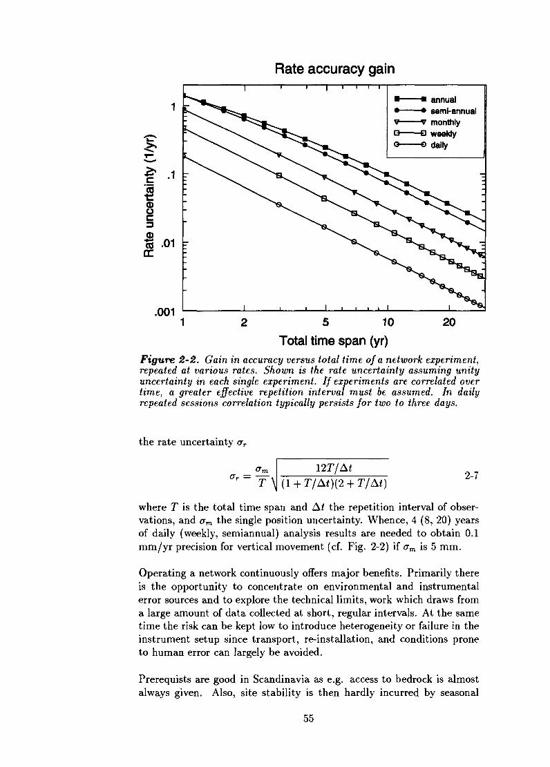
Rate accuracy gain

t8

IS -01DC

.001

annualsemi-annualmonthlyweeklydaily

10 20

Total time span (yr)Figure 2-2. Gain in accuracy versus total time of a network experiment,repeated at various rates. Shown is the rate uncertainty assuming unityuncertainty in each single experiment. If experiments are correlated overtime, a greater effective repetition interval must be assumed. In dailyrepeated sessions correlation typically persists for two to three days.

the rate uncertainty oy

ar = T\1271/A*

(1 + T/At)(2 + T/At)2-7

where T is the total time span and At the repetition interval of obser-vations, and <7m the single position uncertainty. Whence, 4 (8, 20) yearsof daily (weekly, semiannual) analysis results are needed to obtain 0.1mra/yr precision for vertical movement (cf. Fig. 2-2) if crm is 5 mm.

Operating a network continuously offers major benefits. Primarily thereis the opportunity to concentrate on environmental and instrumentalerror sources and to explore the technical limits, work which draws froma large amount of data collected at short, regular intervals. At the sametime the risk can be kept low to introduce heterogeneity or failure in theinstrument setup since transport, re-installation, and conditions proneto human error can largely be avoided.

Prerequists are good in Scandinavia as e.g. access to bedrock is almostalways given. Also, site stability is then hardly incurred by seasonal

55

ground water fluctuations or other problems typical for thick, diageneti-cally unsolidified sediment layers.

2.4.4 VLBI AND GPS TOGETHER

GPS observation points have been established in close colocation with allgeodetic VLBI observatories. The European VLBI baselines now includeNy Alesund, Spetsbergen. Spetsbergen contains another postglacial re-bound centre within the European plate. Horizontal motion within thesubnet of colocated VLBI and GPS sites is prospectively sensitive toFennoscandian rebound owing greatly to the existence of the sites at On-sala and Ny Alesund. However, long records entirely in the same platewith no major tectonic zone intervening exist only for the baseline Onsalato Wettzell.

The colocated sites define an outer network and provides constraints onthe large spatial scale, actually in two ways: (1) colocated techniques ata number of sites will mutually strengthen parameter solutions; (2) infer-ence of motion in post-analysis interpretation will also obtain contraintsfrom the large-scale network.

56

HISTORICAL REVIEW: ONSALA

Geodetic research at the Onsala Space Observatory was introduced byVery-Long-Baseline Interferometry (VLBI). It has been the main compo-nent of the space geodesy research program for more than two decades.The first geodetic VLBI experiment to Onsala, using the Mark-I dataacquisition system at the 25.6 m antenna, was carried out in April 1968(Whitney, 1974). This was actually the first experiment using the band-width synthesis technique (Rogers, 1970). The results from the Mark-Iexperiments have been summarized by Ryan et al. (1986).

The first experiment using the Mark-III system at Onsala was carriedout in November 1979. This experiment had only two channels recordedat S-band (and five at X-band) and it turned out that it was impossi-ble to obtain accurate ionospheric delay corrections. In July 1980 thismistake was corrected (three channels were used at S-band and four at X-band) and the precision of the estimated intercontinental baseline lengthsreached the cm-level. In this first experiment and in many to follow dur-ing the next seven years the X-band was received at the new radome-enclosed 20 m antenna, whereas S-band reception stayed at the larger,old telescope 600 m west of the new one.

Thereafter, many improvements have been added to the geodesy VLBItechnique. Below we will discuss the most important ones, and whenthey were implemented at Onsala. We will also summarize the VLBIobservations so far carried out at Onsala during the Mark-III era and givea couple of examples of the geodetic results from the these experiments.

In this chapter we will also review in short the GPS activities until thebuilding-up of SWEPOS. This latter phase will instead be covered inchapters 4 and 5 of this report.

Towards the end of this chapter we report on recent occupations byabsolute and relative gravimeters at the Onsala site. These independentmeasurements are important for the interpretation of the variations ofthe local vertical position inferred from the space geodesy techniques ofVLBI and GPS.

3.1 VLBI—Technical developments at Onsala 1980-date

3.1.1 The telescopes and the feeds

The original Mark-III setup was to use the 25.6 m antenna for receptionof the S-band signals and the 20 m, radome enclosed, antenna for the X-

57

band signals (Lundqvist, 1984). Because the 25.6 m antenna could notoperate during wind speeds >13 m/s a significant part of many experi-ments was lost at Onsala. Therefore, the S-band operation was moved tothe radome enclosed 20 meter telescope in March 1987 using a dichroicsurface design to allow for the two (S- and X-band) beams to be pointedin the same direction. A couple of years later, the feed system was im-proved using a new design of the dichroic surface (Jaldehag, 1992).

A large upgrade of the 20 m antenna performance started in 1991 whichincluded a new drive system allowing for faster slewing rates and newpanels of higher surface accuracy. The new steering system, includingnumerically controlled motors, resulted in slewing speeds of 2.4 °/s inthe azimuth coordinate and 1.0 °/s in the elevation coordinate comparedto the previous 0.83 °/s in both coordinates. The actual maximum speedsare significantly higher but the new values take into account part of theacceleration and retardation cycle. The rest of this effect is taken careof by the "setup" times in the scheduling program. The improvement ofthe rms surface accuracy from approximately 0.23 mm to 0.13 mm haslittle impact on the S/X-band aperture efficiency (« 0.5% improvementat 9 GHz). The first experiment using the new drive system was carriedout in January 1992.

A second part of the antenna upgrade is still in the design phase. Thismay result in two new subreflectors—one smaller for high frequency radioastronomical observations and one larger for S/X-band observations—and the goal is to significantly improve the aperture efficiency of theantenna at both S- and X-band. The present design has been evaluatedin detail by Jaldehag (1992) and Jaldehag et al. (1993).

In 1980 parametric amplifiers were used at both X- and S-band, withtotal system temperatures, including a typical atmospheric contribution,of 180-200 K and 80-90 K, respectively. Cooled FET amplifiers wereinstalled in the 20 m telescope in September 1986 reducing the totalsystem temperatures to 80-100 K and 50-65 K, respectively. At first,only the X-band part was used but after the move of the S-band to thistelescope in March 1987 (mentioned above) also the S-band part of thereceiver could be used.

Cooled HEMT (High electron mobility transistor) amplifiers were in-stalled in the fall of 1991. The total system temperatures in the zenithdirection and for fair weather are now approximately 70-90 K at X-bandand 45-60 K at S-band. The major contributions to these temperaturesare from losses and ground noise pick-up caused by the feed system andthe radome. The HEMT receiver was first used in January 1992.

Concern about the deformation of the concrete foundation of the an-tenna was raised recently. This pillar is 12 m tall and supports the 20 mtelescope. Inside the radome it is exposed to the daily and seasonal tem-

58

perature cycles, which might introduce height variations and tilts on theorder of millimeters and thus introduce bias in diurnal and annual pa-rameters. In December 1994 temperature sensors were placed at strategicpoints in the pillar. The observations are recorded in a small computer.The analysis of one year of data shows yearly variations of 4 mm peak-to-peak. Tilts and daily variations are on the sub-mm level (Carlsson,1996).

3.1.2 The Mark—III data acquisition system

Compared to the first Mark-III setup at Onsala in November 1979, an-other 7 channels (video converters) were added to the previously incom-plete system before a VLBI campaign in June 1982. Since then thestandard setup has been to record 8 channels at X-band and 6 channelsat S-band.

A high density tape drive was installed in September 1990. The result ofthis improvement was that the number of tapes needed for an experimentwas reduced with a factor of twelve.

The maximum possible spanned bandwidth was increased when theHEMT amplifiers started to be used in January 1992. This upgrade alsorequired an additional IF distribution unit (often referred to as IF3). Thewide band recording mode at X-band presently spans 720 MHz whereasthe standard setup is 360 MHz wide.

3.1.3 The water vapour radiometer (WVR)

Microwave radiometry has been used continuously during VLBI experi-ments since the first successful Mark-III campaign in July 1980 in orderto provide independent estimates of the excess propagation path causedby atmospheric water vapour (Elgered, 1993). Instrumental comparisonshave been carried out at the Onsala site with the NASA owned J03 WVRin the summer of 1988 (Kuehn et al., 1993) and with two WVRs fromETH, Zurich, during October 1992 (Biirki and Elgered, 1993).

The impact of using WVR data for correction of the wet propagationdelay has been studied for the experiments carried out during the pe-riod 1980-1990 (Elgered and Davis, 1993). A couple of examples fromthis study will be presented below in the section on VLBI observations(Figures 3-1 and 3-2).

The WVR was upgraded during the time from October 1990 to Febru-ary 1992. Instead of controlling the data acquisition from the Mark-III"Field System" computer a more flexible, PC based, system was built

59

which allow faster slewing and more frequent data sampling. This is anadvantage in general but especially it will imply improved estimates ofspatial gradients in the wet delay (see, e.g., Davis et al., 1993).

3.1.4 Observations

We will give a brief summary of the geodetic Mark-III VLBI experimentscarried out at the Onsala Space Observatory from 1980 through Novem-ber 1995. Table 3-1 lists the baselines observed to the Onsala site and,thereafter, we comment on the different networks with Onsala participa-tion. We have included experiments with data of acceptable quality frommore than half of a 24-hour session. Another twenty or so experimentswere planned, or only partly carried out, during this period. Most ofthese were lost due to strong winds before March 1987 when the S-bandoperation was moved to the radome enclosed 20 m telescope. After thatdate it has mainly been problems with the antenna drive system or thehydrogen maser that have forced us to cancel observations.

Individual campaigns

We detail a subset of campaigns with a primary focus on geodesy. Thefirst group is devoted primarily to plate tectonics and the second group(MERIT ff) to earth orientation.

US—Onsala, 15 experiments, 1980-1983, was the first network observedusing the Mark-III system including Haystack, Fort Davis, Owens Val-ley, and NRAO in the US and Onsala in Sweden. These were the firstmeasurements of contemporary motion between the North-American andthe Eurasian plates (see, e.g., the early paper by Herring et al. (1986a).From 1983 to 1987, 27 experiments continued on this baseline under theTRANS-ATLANTIC title with emphasis on monthly experiments indifference to the earlier long-duration campaigns once to twice per year.Wettzell was added in January 1985 and Westford replaced Haystack inMay 1985. The 11 NORTH-ATLANTIC 1984-1987 sessions extendedTRANS-ATLANTIC with the addition of Fort Davis, Owens Valley, andlater on Mojave. Here, a deformation transect of the North Americancontinent was obtained. Successor projects along this line were EAST-ATLANTIC, 7 experiments 1988-1989 (Westford, Onsala, Wettzell,Richmond (Fl.), Medicina (Italy)), and WEST-ATLANTIC, 3 exper-iments 1988, (Wettzell, Onsala, Westford, Mojave, and Fort Davis).

Between 1985-1995, 14 POLAR-N have been carried out approxi-mately twice per year, involving Fairbanks, Westford, Kashima, Mojave,Wettzell, and Onsala. The network configuration has slowly changedover the years and in 1993 the sites were: Fairbanks, Westford, Kashima,

60

Table 3-1. VLBI baselines including Onsala measured at least three times during1980-1995 using the Mark-IH system.

Onsala to

Haystack, MA, USA

MRAO WV USA

Owens Valley, CA, USA

Fort Davis, TX, USA

Effelsberg, Germany

Chilbolton, England

Westford, MA, USA

Mojave/DSS15, CA, USA

Wettzell, Germany

Richmond, FL, USA

Fairbanks, AL, USA

Kashima, Japan

Medicina, Italy

Madrid, Spain

Noto, Italy

Troms0, Norway

Metsahovi, Finland

La Silla, Chile

Matera, ItalyL' L . . D . . I , U l I TO A

Fort Davis (VLBA), TX

Los Alamos (VLBA), CA

Mauna Kea (VLBA), HI

Algonquin Park, Canada

Ny Alesund, Spetsb

Hartebeesthoek

Crimea, Ukraine

Total"

80

19

17

16

7

-

-

-

-

-

-

-

-

-

-

-

-

66

81

8

4

9

-

5

-

-

-

-

-

-

-

-

-

-

-

-

-

30

Number

82

8

10

11

-

12

-

-

-

-

-

-

-

-

-

-

-

-

-

45

83

7

-

11

1

11

-

4

1

-

-

-

-

-

-

-

-

-

-

35

84

7

2

10

-

10

1

9

5

-

-

-

-

-

-

-

-

-

-

44

of baseline

85

3

3

11

-

19

5

21

8

2

2

-

-

-

-

-

-

-

-

74

86

1

3

13

-

23

5

23

10

2

2

-

-

-

-

-

-

-

2

84

87

_

3

14

-

23

5

21

11

2

2

-

-

-

-

-

-

-

2

83

measurements

88

15

-

21

5

20

16

2

2

5

-

-

-

-

-

-

1

87

89

_

-

13

-

16

-

23

13

1

1

1

2

1

3

4

-

-

-

78

90

1

-

12

-

14

1

15

12

2

2

3

3

3

-

-

3

2

1

74

91

2

-

-

-

8

8

11

8

2

1

4

3

1

-

-

-

2

-

50

per

92

2

-

1

10

10

25

1

2

2

7

5

2

4

-

-

5

-

76

year

93

1

-

-

1

15

1

24

-

21

1

4

3

1

-

-

-

9

11

11

6

-

-

120

94

_

-

-

2

12

2

15

-

12

2

8

4

2

-

-

-

5

i n

i n

10

9

4

-

6

106

95

_

-

-

1

11

1

13

-

12

1

6

9

4

-

-

-

4

in

g

g

i

7

2

4

98

Total

59

g

42

135

13

7

210

44

224

85

60

18

38

29

14

7

4

3

27

9 7

27o

6

11

8

10

1150

The low number of baselines measured during 1991 was caused by extensive upgrade work on the 20 m telescope(making it impossible to operate the antenna for long periods during September, 1991 — March, 1992). Becauseof the European mobile VLBI campaign during the summer of 1992 there was still a relatively large number ofbaselines observed this year.

61

Medicina, and Onsala. The purpose of these experiments is to tie sites to-gether around the pole and thereby also different VLBI networks whichtogether include sites that have poor common visibility of the extra-galactic sources.

The dedicated EUROPE network—including Noto, Matera, Medicina,Madrid, Wettzell, and Onsala—started to observe in 1990 and has beenscheduled 3-6 times per year, currently with a record of 23 experiments.Additionally, the Effelsberg antenna has been used occasionally duringthe last couple of years. The geodetic results from these experimentshave been proven to be of high quality (see, e.g., Rius et al., 1992).

An effort of EUROPE MOBILE experiments proceeded 1989, 1992,and 1993 with 22 sessions. During the summers of 1989 and 1992 Onsalaparticipated as a base station to support the MV-3 and MV-2 occupa-tions at different European sites. Metsahovi and Troms0 was observedby MV-3 in 1989 and Kirchberg, Karlsburg, H0fn, and Troms0 by MV-2in 1992. Furthermore, in May 1992, one 24-hour experiment was madewhen MV-2 was located at the Onsala site, approximately 20 m from thepermanent GPS tracking station. The vector estimated from the VLBIdata has formal one-sigma errors of 2 mm in the horizontal componentsand 4 mm in the vertical component (Potash, 1992). The disagreementswith conventional surveys and GPS measurements are 2-3 times as large.In January 1992 and in March 1993 Onsala also participated in IRIS-Aexperiments which included the mobile station MV-2 at Trysil, Norway.

A geodetic baseline between Onsala and the SEST antenna on La Silla inChile was measured a few times during April and May 1990 (Jaldehag,1992).

MERIT, 14 experiments, 1980 (Monitor Earth-Rotation and Intercom-pare the Techniques) "short campaign", during two weeks in Septemberand October 1980, used the US-Onsala network and alternatingly Ef-felsberg in Germany and Chilbolton, England, as additional stations inEurope.

The 29 POLARIS (POLar-motion Analysis by Radio InterferometricSurveying) experiments 1980-1984 had the major goal of study earthorientation monitoring. In the beginning an experiment was carried outevery second week. Originally only the Haystack and the Fort Davissites were regularly available and it was only when a third station joinedthe network that it was possible to estimate all three earth rotationparameters (the x- and y-components of the pole and the rotation rate).Onsala participated approximately once per month. Westford replacedHaystack in 1981 and then the experiments were scheduled once a week.The Richmond site in Florida was added to the network and participatedon a regular basis starting in 1984.

62

The IRIS-A experiments, 90 in number during 1984-1993 continuedPOLARIS, scheduled at every fifth or seventh day. As in the PO-LARIS network Onsala has participated in these experiments regu-larly (approximately once per month). The stations in the networkhave varied but most often they were: Westford, Richmond, and FortDavis/Mojave/Fairbanks, in the US, and Wettzell in Germany. The FortDavis antenna in Texas was closed in 1989 and replaced by Mojave inCalifornia. Mojave in turn was closed in 1992 and replaced by Fairbanks,Alaska.

Starting in May 1993 the IRIS-A experiments were replaced by NEOS-A and NEOS-B experiments, 15 sessions 1993-1994 (NEOS = NationalEarth Orientation Service). The NEOS-A observes once per week usingan identical network each time which makes it impossible for stationssuch as Matera and Onsala to participate on a monthly basis. Instead aseparate network, NEOS-B, has been defined which observes at approx-imately one month intervals. The stations used have been: AlgonquinPark, Fairbanks, Green Bank, Matera, Onsala, and Wettzell. As a side-effect of NOAA passing responsibility for NEOS to USNO, NEOS-B hasbeen discontinued at the beginning of 1995.

As plate tectonics studies shifted towards regionally more refined projectsVLBI obtained the role of a large-scale network stability custodian. Thisthe border between earth orientation and plate tectonics appliciationsstarted to disappear. In this context NASA's R&D Network has beenoperating, comprising 27 monthly experiments since 1993. The 1995R&D network consisted of Fairbanks, Fort Davis (VLBA), Kokee Park,Los Alamos (VLBA), Onsala, Westford, and Wettzell, i.e. an exceedinglyglobal network, striving for pushing the limits of parameter estimation ofboth baseline vectors and reference system orientation. By coordinationwith NEOS, NAVEX and VLBA, two week-long CONT sessions havebeen performed in 1994 and 1995, in which Onsala was observing duringthe whole time span. The purpose of the CONT sessions is to assess theconsistency individual VLBI-networks as regards short-term variationsprimarily in earth rotation. Discussions on the demonstrated repeatabil-ities using different networks have been presented by, e.g., Rogers et al.(1993) and MacMillan and Ma (1994).

Onsala participation currently

By the beginning of 1996 Onsala participates in the CONT, EUROPE,and GTRF networks. The typical precision of estimated baseline lengthsis now well below 1 cm and the typical repeatability of estimated trans-atlantic baselines is at the 1 cm level over time periods of many months.

63

3.1.5 VLBI results

Results from the two most frequently observed baselines to Onsala areshown in Figure 3-1 (Onsala-Wettzell) and Figure 3-2 (Onsala-Westford)together with NUVEL-1 predicted rates for the time period 1982-1995.

Results are presented for the baseline to Westford in Figure 3-3, demon-strating the difference in the analysis between the use of WVR data andestimating a Markov process for the wet propagation delay at the Onsalasite (Elgered and Davis, 1993). Here we have used only that subset ofthe solutions which were analyzed with roughly the same methods (untilthe hardware change in WVR October 1990).

In each method an optimum elevation cut-off angle is determined bythe criterion to minimize the weighted RMS of the fit. These cut-offangles are wastly different. Using WVR data, the inferred wet delay isaccurate primarily at high elevations, giving an optimum cut-off between17 and 20°. Estimation of the tropospheric delay from the observationsthemselves, on the other hand, requires low elevations down to 5° as thesecarry the effect most strongly.

In general we conclude that the formal one-sigma uncertainty of theestimated baseline lengths as well as the repeatability improve with timeregardless of which method is used for the atmospheric corrections atOnsala. It is seen that the short time repeatability is much better thanthat over longer time scales. The impact of using WVR data is a loweringof the error level mostly during the later periods, presumably in thecourse of other critical error sources having been brought under control.

In the case of the baseline to Wettzell we note that the estimated rates are-0.2±0.2 (la) mm/yrfor the WVR solution and -0.7±0.2 (1<T) mm/yrfor the Markov solution. The expected change in the baseline length dueto the postglacial rebound is of the order of —1 mm/yr (Onsala towardsWettzell) (Mitrovica et al., 1994). Clearly systematic errors prevent usfrom claiming to have detected such a motion today.

The Onsala-Westford baseline is more than six times longer than thatto Wettzell and is, therefore, more affected by atmospheric errors as thelocal verticals at the endpoints project more into the baseline's lengthcomponent (Herring, 1986)). Systematic effects in the estimated baselinelengths are clearly seen in the WVR solution, c.f. Figure 3-3. The esti-mated rates are 17.6±0.3 {la) mm/yrfor the WVR solution and 14.8±0.3(la) mm/yr for the Markov solution. If we, however, only use the 1988—1990 data both rate estimates are consistent («20±2 (la) mm/yr) andin reasonable agreement with the geological estimate from the NUVEL-1 model («18 mm/yr) (DeMets et al., 1990). The solution using theMarkov process and elevations larger than 5° gives a weighted rms of theresiduals of 13.7 mm for the whole data set (133 exp.) and 11.8 mm for

64

VLBI Onsala Wettzell

1980 1985 1990Time [yr]

1995

Figure 3-1. Estimated baseline lengths Onsala-Wettzell in the threeorthogonal baseline components, Length, Transverse, and Up. (The planespanned by Length and Up contains the geocentre.) This is the GSFCstandard solution, not using Water Vapour Radiometer (WVR) data norusing a Markov process to estimate wet tropospheric delays from the data.The weighted rms of fit for each component is 3.6, 3.3, and 13.7 mm,respectively. Using WVR data, the estimated Length rate changes from0.6 ±0.1 mm/yr (dotted line) to 0.25 ±0.1 mm/yr. Shown are also therates predicted from NUVEL-la plate motion (dash-dotted lines)

65

VLBI Onsala Westford300

-1001980 1985 1990 1995

Time [yr]

Figure 3-2. Estimated baseline lengths Onsala-Westford. This is theGSFC standard solution. Shown is also the rate predicted from NUVEL-la plate motion (dash-dotted line) and the mean observed rate (dottedline), 16.9 ±0.2 mm/yr.

the last three years (42 exp.). When the WVR data are used a largerelevation cutoff is adopted (20°). In this case we obtain a weighted rmsof the residuals of 13.8 mm for the whole data set and 10.4 mm for thelast three years.

3.2 GPS—1986 to 1993

Operations with receiver equipment for the Global Positioning Systemstarted at Onsala in conjunction with the Iceland campaign summer 1986(Rothacher and Beutler, 1988). At this occasion Onsala was selected asa fiducial site. Since colocation with a well-established VLBI point wasfeasible, the observations with a TI4100 receiver at Onsala would tiethe Iceland network into the International Terrestrial Reference Frame(ITRF). Similar high-latitude fiducial sites were maintained at AlgonquinPark and at Westford. The deployment of satellites was by far incom-plete, and the network suffered from a low number of simultaneouslyvisible space-craft.

The fiducial site concept was developed further, converging into the es-tablishment of a world-wide infrastructure of today, the Internations GPSService (IGS). A major stage leading there was CIGNET (CooperativeInternational GPS Network), a network of permanently observing GPSreceivers colocated at VLBI or SLR sites and thus tied into the ITRF.The CIGNET station at Onsala was put into service in December 1987.After a couple of monument changes and relocations of the antenna, aconcrete 1 m high pillar has been the permanent place for the CIGNET

66

I1-6!

§

8_j 1.4 ^

1.3

I 1 6

O 1 0

oCO

Jj 1.4

1.3

VLBl bnsala Westford, Markov

VLBl Onsala Westford, WVR

1980 1985Time [yr]

1990

Figure 3-3. Estimated baseline lengths Onsala-Westford, using astochastic filter (Markov method) or Water Vapour Radiometer obser-vations (WVR) to reduce the propagation delay due to variations in at-mospheric water vapour. Wastly different elevation cut-off limits arerequired in each case to obtain minimum rms of the residuals (WVR 20°,Markov 5°). The observed baseline rate turns out to be sensitive to themethod, 15.0 mm/yr resp. 17.6 mm/yr, more details see text. Using theWVR the residual shows less rms and systematic signatures, which mayar may not be of atmospheric origin. The Markov-modelled troposphereis suspected to falsely pick up such systematics.

67

point. Today it is used as the primary antenna point for the permanentoperations in both SWEPOS and IGS.

A number of support points have been founded, and local ties have beenmeasured to establish and maintain the coordinate ties to the differentreference systems (Swedish national RT, Nordic NORDREF, EuropeanEUREF, World WGS) and between the VLBI and GPS ground referencepoints (Johansson et al., 1992).

Today, Onsala is a core station of the IGS network. The satellite obser-vations have also been used in research and development projects carriedout by various companies for the purpose of navigation and rapid differ-ential positioning.

Recent developments concern providing estimates for the wet propaga-tion delays from GPS measurements, comparing these results with thosesimilarly derived from VLBI, and with independent WVR observations ofthe thermal emission from atmospheric water vapour. Research on GPSantenna design, radiation fields and scattering effects will be mentionedbelow in the SWEPOS context.

The photograph in Figure 3-4 shows the VLBI-facility, the GPS monu-ment, and the water vapour radiometer.

3.2.1 Gravity measurements

The GPS observation cabin at Onsala is built around a concrete groundplate furnished for gravimeter observations. Several occupations by ab-solute gravimeters have occurred during 1992-1994. The first visit wasby the Swedish National Land Survey in November, 1992. The next ob-servation period used the absolute gravimeter of the Finnish GeodeticInstitute in March 21-23, 1993. Two absolute gravimeters from NO A A(FG5 102) and IfAG (FG5 101) [Klopping et al., 1991] occupied the siteduring August 7-10, 1993. A remeasurement with the NOAA instru-ment was carried out September 28-29, 1995. Gravity gradients alongthe gravimeter bed have been surveyed by Jakko Makinen of FGI Helsinkiin April 1995. Another visit occurred on May 16, 1994, from "Kort ogMatrikelstyrelsen", Denmark.

3.3 FUNDING

Geoscience and related research at Onsala Space Observatory is to thelargest extent basic research. Support for the establishment of the tech-nical facilities and the localities has been granted by Knut and AliceWallenberg's Foundation and the Swedish Council for Planning and Co-

68

Figure 3-4- Facilities at Onsala Space Observatories include the 20 m radio tele-scope for \ LBI (covered with the large radome), the water vapour radiometer (lefthand side, foreground), and the GPS antenna monument on thf square pillar to theright. Another 20 m to It ft outside thi picture is the hut housing the GPS receiverequipment and the measurement platform and reference points for gravity. Located athalf this distance is a reference point for large mobile geodetic instruments like \ LBIor satellite laser ranging equipment. (The device in the foreground is a test assemblyof em ESRANGE rocket element on which a GPS antenna has been mounted.)

ordination of Research (FRN). Projects have been funded by the SwedishNatural Science Research Council (NFR) and the Swedish ResearchCouncil for Engineering Sciences (TFR). Together two European Com-munity and European Union (EU-S(TENCE) projects have been sup-porting specific projects in conjunction with VLBI. GPS, and WVR.

Thanks to long-term loans by and unbureaucratic exchange with NASA,VLBI equipment has been kept operating in healthy conditions duringmore than fifteen years.

The radio telescope itself is supported by the government as the SwedishNational Facility for Radio Astronomy.

69

GPS NETWORKS

In the following discussion of GPS networks we will consider only thosethe aim of which is to monitor movement at the centimetre to millimetrelevel. This has become feasibe technically. In comparison to VLBI asthe still most precise technique, the precision gap to GPS is less than anorder of magnitude, but the costs involved in creating and operating anequivalent VLBI network would be more than two orders of magnitudegreater.

Among different concepts to operate GPS networks we may distinguishaccording to the degree of activity

• field campaigns, re-occupation at monuments, mobile instrumen-tation incl. antenna support (e.g. tripods);

• permanent installations, but data retrieval and analysis sparsein time;

• continuously operating, retrieving and analyzing as much dataas can possibly be observed.

The first type requires a high level of manpower and runs risks of technicalproblems in the course of the field work, which will put limits on thenumber of network nodes. The second set can avoid these problems; alarge number of sites may be included in simultaneous network solutionssince long periods of time can be expended in the data processing phase.In the third type the number of network sites is traded off against thegain in precision offered by producing dense time series of solutions. Alsothe cost per data point is minimized.

Analyzing daily sections of GPS data each 30 h long, we find that indi-vidual position determinations decorrelate statistically already after twoto three days. Thus, 24 h to 48 h solution intervals already contribute toimproving the stability of estimated mean positions and rates of change.The search for transient perturbations can be extended to these shorttime scales.

Once the decision converges towards establishment of a permanent net-work, a large number of organisational details need to be resolved. Thenumber of sites to be included will have a lower limit imposed by theapplication. The required data throughput will determine the data fa-cilities for acquisition, processing and archiving, and some trade-off canbe achieved by simplifying or sacrificing certain phases of the computingprocess (like obtaining satellite orbits from a central service) while theamount of data would facilitate the attenuation of errors.

70

Ultimately the success of the system as a whole will depend upon anassemblage of individual features and technical/logistical/infrastructuraldetails. A large number of decisions is needed to optimally tailor andfine-tune the system, cf. Chapter 6.

The detailed technical specifications for SWEPOS sites are given in thefollowing sections. We estimate the additional cost for adding one stationto be 0.5 MSEK (that station would include one receiver and no RTCMservice, but else have the same quality as a standard SWEPOS station).

4.1 TECHNICAL REQUIREMENTS FORPERMANENT OBSERVING SITES

Permanent operation of observing sites causes a number of consequencesconcerning the installation of the basic equipment, supporting equip-ment, and infrastructure.

The minimum equipment required to carry out observations within a lim-ited period of time, say from some hours to a couple of days, would consistof an antenna, a receiver, data recording media, and battery power. At aminimum the site would be established by installing a permanent geode-tic marker (brass bolt) in a large outcropping boulder or an accessiblebedrock surface. The antenna could be placed on a tripode and the ec-centricity between the antenna's reference point and the geodetic markerbe measured to within one millimetre.

Many surveys have been carried out using this minimum setup. Ad-ditionally, observations of air temperature, pressure and humidity haveoftentimes been made as processing software containing options to modelthe signal delay in the troposphere may accept such data. The usefulnessand representing power of near-surface meteorological data, however, ishighly debatable.

Permanent installations raise concern about the inherent stability of thesystem. The reference point of an antenna, the point to which the geode-tic determinations are effectively been made, will in general differ fromthe reference marker by the site tie. The site tie (and the monument it-self) will not be ultimately stable and thus will affect the position of theantenna reference point. But seen from the electrical point of view theantenna reference point is an abstraction; it is an effective position giventhe actual distribution of angles of the incident waves and the actualeffect of wave scattering and other signal perturbations in the antennaassembly and its environment. Thus, in both the aspects of mechani-cal and electrical reference point stability, possible routes of attack mayconsider to (i) avoid or at least suppress, (ii) to compensate and (iii) tosurvey and model the pertubations.

71

Permanent sites necessitate stable structures to support the antenna, acabin to house the receiving equipment and peripherals, and infrastruc-ture to provide electrical power and to off-load the recorded data. Thissection will present general points of view considering critical propertiesand trade-offs to be resolved in the planning of observing stations. Fur-ther down we will present the SWEPOS solution, its benefits and itslimitations.

4.1.1 Antenna support structures

Satellite observing sites are preferably located in areas remote from cities,industry, mines, electrical power lines, roads, and railways for a numberof reasons. Tall standing structures may not obscure the antenna horizon.Metal surfaces in the antenna environment may not reflect the incomingwaves causing nonstationary multipath or scattering conditions. Inflici-tions on ground stability must be avoided. The permanence of the sitemay not be limited for a forseeable future due to infrastructural devel-opment, land-fills or exploitation for e.g. ground water.

For the purpose of

• staying clear from a ground snow cover,

• standing out of reach of animals and humans

• extending the horizon mask

the antenna is preferably mounted on a standing structure, e.g. a con-crete (rock, ceramic ...) pillar or a metal framework tower. Typicallysuch a structure will have to be between one and several metre tall. Ex-posed to the seasonal thermal cycle and exposed to the daily insolationand thermal cycles, the structure will undergo deformations which — inthe present context — may be considerable. Also, concrete will expandin reponse to increasing humidity, but tailered composition and surfacetreatment can limit these effects.

• A minimum of perturbing objects in the field of view ofthe antenna.

Preventive measures are required to keep the antenna itself clean fromsnow and other objects that may settle on its top or accumulate at placeswhere they perturb the antenna radiation field. The required protectionis usually accomplished with a plastic or glassfiber radome. The radomeshould shield off the antenna to all sides. Its material must be chosen

72

with care, i.e. the refractive index in the 1.2 to 1.6 GHz frequency intervalshould be low. The shape and a low surface roughness of the radome isto be designed to counteract raindrop and snow adhesion and snow andice pile-up. Birds should be discouraged from perching, which can beaccomplished attaching a sharp spike on top.

• The structure must be stable.

The antenna support must be resistive to wind loads, preventing defor-mation beyond the one millimetre level. It must withstand frost. Ad-ditional stabilization (temperature control, thermal compensation) mustbe considered in order to maintain a sub-millimetre limit on tempera-ture induced movements within the mount assembly. Firm mechanicalcoupling of the monument within the bedrock environment is required.Means and measures for monitoring eventual movement of the antennawith respect to the ground are required in order to assess the long-termstability.

• A standard structure should be adopted.

Analysis has shown that monuments at a height of at least two metresimply an effective averaging of multipath perturbations due to the re-flections from the ground as the satellites move over the daily range ofelevations (Elosegui et al., 1995; Jaldehag et al., 1995; Jaldehag andYing, 1995). The phase variations induced in the received signals is anoscillating function of satellite elevation, the number of zero-crossings inan elevation interval being largely proportional to the monument height(for details cf. Chapter 4.1.2).

However, the antenna mount, the design of the top of the pillar, andthe structures at decimetre distances from the antenna may cause largemultipath perturbations with much fewer zero-crossings over the satel-lite elevation interval, causing considerable systematic error in the dataanalysis. The studies suggest that identical structures (monuments andmounts) inflict the smallest systematic errors, and thus that the monu-ments can favourably be produced in a series. This goes hand-in-handwith the economy of the project.

A wide range of solutions exist in the precision networks, from tripode-like leg supports (the UCLA Piniion Flat model) via metal framework(FGI, Finland) to concrete and stainless steel pillars (GSI Japan). As allof these projects are new, evaluation of monument and mount stabilityand determination of the optimum design at this point of time would bepremature.

73

The Working Group on Permanent Networks of the Nordic GeodeticCommission is on the way to define such a standard in order to facilitatehomogeneous network solutions when sites within the different subnetsare combined.

• Horizon mask must permit visibility above 10° elevation.

Satellites need to be tracked to elevation angles typically down to 15°above the horizon. In network analysis, common visibility from all sta-tions will strengthen the results, but at least one pair is required. Ob-servations at low elevation angles are required to increase the resolutionpower of site height and the troposphere parameters. Considering thecarrier frequencies of the GPS signal, practically all kind of buildings(wooden, stone, ...) and all kinds of conducting material will block orseverly attenuate the signal. Even thin layers of metal will block thesignal, and thin sheets of plastics or other dielectric material (plant'sleaves) will perturb the signal or at least introduce undesired delays andscattering patterns.

Thus, material from which antenna covers can be made must be chosenwith care.

Considering the preference for a remote location of sites, this impliesthat sufficiently open areas must be found or trees and other vegetationaround the antenna monument must be clipped. Raising tens of metrestall structures, however, is less feasible as these would be even moresusceptable to thermal variation and wind loads.

The cabin will generally not inflict on the horizon mask if the monu-ment has a height of three metres or more. However, near-by locationof the cabin may imply reflection of the GPS signals from the roof andintroduce a multipath problem. For countermeasures the gable of thecabin should face the monument, and the distance to the monumentshould be sufficient, e.g. 10 m (most sites) appears better than 1 m (atFuruogrund).

The solution preferred in Finland (Vermeer, 1994) devises a steel frame-work tower 3.0 m tall. At Metsahovi the tower is 8 m tall and is compen-sated for thermal expansion by an Invar-steel rod. This rod effectivelyclamps the antenna mount to the monument base very near the geodeticground reference marker, while the steel tower provides the horizontalsupport.

74

4.1.2 Antennas

Using antennas of different designs within the same network can intro-duce serious site-to-site heterogeneities in receiving conditions. Schuplerand Clark (1991) and Schupler et al. (1994) specify correction methodsfor experiments which mix different antenna types. The major conclusionof the recent work of Jaldehag (1995) is to use antennas of identical typethroughout the network. Reducing the errors due to different antennasby using a model to describe the sensitivity patterns is considered as a toouncertain method. Still, the particular antenna type which introduces anacceptably low level of perturbations needs careful consideration.

The sensitive antenna element consists usually of two dipoles, arrangedcrosswise in the horizontal plane. The dipoles are electrically coupled forcircular polarization. This arrangement obtains omnidirectional sensitiv-ity in azimuth and approximately cosine sensitivity with respect to thezenith angle. The main lobe of a simple dipole at finite distance abovea finite ground plate extends to angles below the horizon. At still largerangles perturbations are admitted through the sidelobes of the radiationpattern.

Owing to the design of the antenna assembly, particularly enhancedground plane models, scattered or reflected waves impinging on the an-tenna dipoles at sub-horizon angles can be attenuated with high ratios.

One of these antenna types, the choke ring design, obtains an enhancedground plane by virtue of deep, concentric metallic corrugations. Theirattenuating effect must be tailored to fit the particular frequencies. Themethod works strictly only at one frequency. Already with two frequen-cies modelling criteria and trade-offs become considerably complex, yield-ing many different design options (number of choke rings, vertical profile,horizontal spacing). A number of technical solutions have been realizedand are available from antenna manufacturers.

A widely used GPS antenna is based on the cross-dipole assembly orig-inally designed by JPL and manufactured by Dome & Margolin, N.Y.Suppliers of GPS equipment add a choke ring and preamplifier assem-bly. Chocke ring antennas have become the standard choice for AllenOsborne's TurboRogue and recently also Ashtech receivers. The follow-ing variants exist: Original DM-T, a DM-TA type, and an older DM-Bmodel. They are practically identical. The DM-TB has a different bot-tom plane housing the pre-amplifier assembly, which has no demonstrat-able effects on the radiation pattern.

The original Ashtech antenna that came with the Ashtech Z-12 or P-12receiver and is similar to the Trimble antenna has been used in SWEPOSonly temporarily.

75

4.1.3 Receivers

For high-precision purposes, receivers must be capable to acquire andprocess both phase and P-code measurements simultaneously for the twofrequencies and for as many satellites as can be visible, which is morethan eight but less than twelve. This restricts the candidate receivermodels to the product palette of about five manufacturers

During Anti-Spoofing, P-code measurements require a sophisticated pro-cedure to derive an equivalent P-code variable from the Y-encrypted sig-nal, which is accomplished by real-time cross-correlation in TurboRogueand Ashtech receivers. Satellite clock dithering under Selective Avail-ability favours the use of receivers with stabilized oscillators, or the useof external Rubidium or Caesium oscillators as an alternative.

An extensive list of receivers and their specifications for a wide range ofapplications is found in GPS World (1996).

4.1.4 Other station equipment

At remotely located sites the following equipment may be considered:Backed-up uninterrupted power supplies; data communication modemsor other connectors to data networks; air heating and/or cooling devices.The use of frequency standards (Rb or Cs time standards) may in thefirst case be indicated in connection with the Ashtech Z12 receiver andits drifting oscillator. Evaluation is under progress.

4.2 THE SWEPOS SITES

Here we describe the actual realisation in SWEPOS of the antenna, itsmonumentation and other site facilities in conjunction with the instru-ment cabin, supposedly meeting the demands above. We will discuss thecases where problems have been detected, the solutions we devised andproblems that might still persist.

A map of the network is shown in Figure 4-3. Figure 4-1 shows SWE-POS along with similar networks in Finland (FinnNet) and Norway(SATREF).

Geodetic positioning solutions in the SWEPOS network with the non-fiducial strategy (c.f. \ref{sec:NONFID}) utilize IGS data observed atseveral sites within Europe, all being located on the same tectonic plateand well separated from active margins. Thus, the regional solutions canbe postfit to the GPS subset of the ITRF which is maintained by theseIGS sites. The small deformations known to exist across the Alps and

76

Pyrenees do not inflict on this strategy. The IGS sites used in the Onsalasolutions together with the SWEPOS sites are shown in Figure 4-3.

4.2.1 SWEPOS sites design and equipment

The SWEPOS pillar

The SWEPOS network is furnished with a standard 3 m tall concretesteel-inforced pillar of circular cross-section. The standard pillar designis due to the National Land Survey (cf. Figure 4-4). The Division ofStructural Mechanics (Doc Ola Dahlblom) at Lund Technical Universityhas assisted in its development with studies on the thermally induceddeformations. The foot of the pillar consists of a 0.75 x 0.75 m concreteplate. The pillar's steel inforcement continues through the bottom plateinto holes drilled into the bedrock. The concrete of the foot plate is castinto a shallow bowl-shaped mould hammered out of the bedrock.

Under an insulating outer cover that extends over the height of the pillarand consists of a helically wound corrugated plastic sheet, rockwool insu-lating material aids in attaining a homogenous temperature field through-out the pillar. The temperature level is controlled attaching a heatingwire to the pillar, helically wound. A temperature sensor is fit into asmall cavity inside the pillar and connects to a thermostat unit in theinstrument cabin (on-off regulator, powered with AC from the mains).

The pillar set temperature is 15 °C. Present temperatures exceeding thislimit may deform the pillar. At 40 °C the length change is still belowone millimetre. Figure 4-5 shows a photograph of the Vanersborg site,which is furnished in the standard design.

Exceptions are as follows: The Jonkoping pillar is a 1 m lowered versionof the standard pillar (for air traffic safety); actual coupling to bedrock isunclear and confirmation would be desirable. Lov6 and Martsbo monu-ments rest on pre-existing pillars with a rectangular cross-section. Onsalacontinues to use the CIGNET monument on a 1 m tall pillar with a squarecross-section (cf. Fig. 4-2).

Local control network

At ten to twenty metres distance from the monument, geodetic markers(stainless steel studs) are driven into the surface of the bedrock. Usu-ally six such markers, as regularly distributed as possible with regard tohealthy bedrock accessibility, form a local network within which eventualdeformations of the top of the antenna monument can be detected.

77

?0

SWEPOS*FinnNet

SATREF*

Figure 4-1. SWEPOS. the Permanent Swedish GPS Network and itsNorwegian (SATREF) and Finnish (FimiNel) neighbours.

78

Figure J^-2. SWEPOS monumtni at Onsala. old radome. Eccosorbmaterial in-line with the antenna bottom plate has been removed for thephoto.

79

SWEPOS^; JIGS°

v ' JGS(n.u.)

I M L ' , 1 1 Mar 8 16:41 | xxx.p»

Figure 4-3. The SWEPOS Permanent Swedish GPS Network and theEuropean IGS sites regularly included ("n.u."—not included) in the so-lutions derived for the DIFROST project.

80

3 _

2. »

s a_ITS a

o -*

Stainless steelplate for antenna

Thermostat andelectrical heatconductor

Circular concretepillar, 0 - 30 cm

Insulatingmaterial

Outer wall

Concrete plate

4 Iron Rods

Side ViewGPS Monument

ConcretePillar

Steelbolt

6 +

1

1

5 +

A

7T

/ V

' \

\

• — **" ^ * "

s.J

- -r "" "• '^0

4

1

**"'•*- « ^ 2

\

\

+ 3

18 m

s

The Local Control Network at Esrange

Top ViewGPS Site

Figure 4-5. The SWEPOS station at Vantrsborg. SWEPOS standardpillar and new radonx

In a control survey, the antenna is removed and replaced with a theodo-lite. The horizontal and vertical angles to the steel studs are observed.The detection level for horizontal and vertical movement of the pillarwithin the control network is 0.1 mm.

The National Land Survey carries out the control measurements. Lek-sand has been used as a control site where the local network has beenobserved twelve times with at minimum one-month intervals during 1993-1995. In general the monuments have been measured and remeasuredonce in two years. Preliminarily, in some cases the surveys seem to indi-cate movements of one to two millimetres.

Independent evidence that helps discriminate interannual and seasonalsignatures from secular trends is considered extremely important. Thestrategies for the local control measurements must suit these needs interms of how regular and how frequent they are carried out. Recovery ofan annual cycle requires that measurements repeat from year to year ona calender basis. On the other hand, the circumstance that the antennamust be removed and an optical observing device be installed in its placeintroduces a source for systematic errors (the remounted antenna mustreturn to the previous position and the parts and pieces must not changeelectrical environment of the antenna). At present we need to developthe strategies for the control surveys further to obtain greater significancewhile simultaenously reducing systematic perturbations.

82

The SWEPOS antennas

All sites are now equipped with Dome-Margolin choke ring antennas.Where stations are furnished with the standard pillar a profoundly ho-mogeneous geometry in the aspect of EM propagation, diffraction andscattering has been achieved.

The shorter pillar and the special antenna mount at Onsala has causedsome concern as to the wave scattering conditions in its near field. Also,the site is just outside our laboratories so that testing alternate arrange-ments is less time consuming. Our experiments have converged to thefollowing solution: Scattering perturbations originating from the mountand backplate structure has been attenuated with the help of EM waveabsorbing material (Eccosorb AN-W). A 61x61x5.7 cm square piece hasbeen put directly above the metallic back plate, yielding satisfactory pre-formance (Jaldehag et. al. 1995b).

Extended antenna choke ring designs have been considered using com-puter modelling, and some have actually been manufactured (Jaldehagand Ying, 1995). The extension concerns the number of choke rings aswell as their thickness profile and spacing.

The SWEPOS radome

After a first winter of experience with a fiberglass radome manufacturedby Delft University, a new design was developped by our group in orderto avoid snow/ice accumulation. Large (40 mm) vertical variations inthe vertical component determinations were observed primarily at theinland sites of northern Sweden. Jaldehag et al. (1995) found correlationwith precipitation and the local temperature at ground-level. The studysuggested that snow was accumulating around the top of the pillar andthe mounting elements of the Delft radome which together present manysurfaces for snow and ice to attach and settle on. The OSO model wasdeveloped from this experience and eliminates edges due to its straightinverted icecream cone design with an aperture wide enough to extendover the top surface of the pillar with an overhang (cf. Fig. 4-5).

Owing to the electrical properties of the radomes, the transition from theDelft to the OSO model induces a detectable, virtual change in the siteposition, generally less than 20 mm in the vertical and smaller than thatin the horizontal. It was found that this change in position is differentat each site and therefore must be determined individually. The variabil-ity is probably related to surface inhomogeneities in the plastic moldingprocess.

83

The SWEPOS receivers

At present all SWEPOS sites house two receivers. Employed models areeight channel TurboRogue and/or twelve channel Ashtech Z-12. Table4-1 shows the currently deployed receiver/antenna combinations at allsites. At stations that house two receivers a power splitter connects bothreceivers to the same antenna. The remainder of this chapter gives ashort historic review.

In the first phase (1993-94) 15 sites were equipped with TurboRogue re-ceivers, all of which connected to DM antennas. At the time AS wasswitched on by the US DoD, the TurboRogue was the only receivermodel capabable of full wavelength L2-measurements. Some stationswere equipped with Ashtech P-12 receivers of which the larger part wasconnected to Ashtech antennas. In order to achieve homogeneity in re-ceiving conditions, which was a primary concern, DM antennas replacedthe Ashtech ones in 1995. From July 1, 1995, all 20 (21) stations couldbe included in the BIFROST data analysis.

Sites that are used for Differential GPS require the full RTCM capabilityand Doppler measurements (for terms cf. Chapter 4.3.4 below). Also,the sampling rates preferred in this application are high. The receivermatching this purpose is the Ashtech Z-12. Presently, 13 of the DGPSreference sites house an additional TurboRogue receiver. A 15 s sam-pling rate is the standard for the data used in the BIFROST analysis.The preference for this receiver, however, has been due largely to its os-cillator being more stable and being controlled in a more suitable way,but recently the increased number of simultaneously visible satellites hasmotivated to favour the Ashtech model.

In order to control the Ashtech oscillator, an external frequency refer-ence is supplied by precision quartz oscillators or Rb clocks installed atLovo and Martsbo. Onsala uses the observatory's hydrogen frequencystandard. On the other hand, the uncontrolled oscillator has not causednoticeable problems.

Instrument cabin

The standard SWEPOS instrument cabin has a size of 3x2 m and houses

• one or two satellite receivers,

• optionally one precision quartz frequency standard,

• one data collecting computer for each receiver (486 PC, typically aLaptop model),

84

• one telecommunication modem for each receiver,

• one modem for remote control of electrical power supply to allinstruments,

• Uninterrupted Power Supply (UPS) including batteries,

• heater control of the antenna pillar

(cf. Fig. 4-6) Thermal insulation helps to maintain the ambient temper-ature range of the equipment, and ventilation safeguards for lead-acidrechargable batteries. Considering an outdoor temperature range be-tween -40 °C and +35 °C, the additional heating effect due to insolationon the cabin's surfaces, and the power dissipation of the apparatus (15W/receiver; 40 W/PC; 40 W/LapTop; 50 W/modem) necessary heatingand cooling devices have been installed.

Power mains and telephone installation must be properly protectedagainst transients, primarily those induced by lightning strikes.

Attendance or visual inspection is done on the average four times peryear.

Table 4-1 Summary of site equipment

site"

Arjeplog (ARJE)Boras (BORA)Hassleholm (HASS)Jonkoping (JONK)Karlstad (KARL)Kiruna (KIRU)Leksand (LEKS)LovS (LOVO)Martsbo (MART)Norrkoping (NORR)Onsala (ONSA)Oskarshamn (OSKA)Ostersund (OSTE)Overkalix (OVER)Skelleftea (SKEL)Sundsvall (SUND)Sveg (SVEG)Umea (UMEA)Vanersborg (VANE)Vilhelmina (VILH)Visby (VISB)

Latitude6

[°]

66.3157.7156.0957.7559.4467.8860.7259.3460.6058.5957.4057.0763.4466.3264.8862.2362.0263.5858.6964.7057.65

Longitude6

H

18.1212.8913.7214.0613.5121.0614.8817,8317.2616.2511.9316.0014.8622.7721.0417.6614.7019.5112.0316.5618.37

Height6

M

489219114260114498478807541461504902238131

4915417045080

receiver(s)c

2 AA + TRA + TRA + TRA + TRA + TR

2 A2 A

A + TR2 A

A + TR2 A2 A2 A

A + TRA + TRA + TRA + TRA + TRA + TRA + TR

pillarc

3-mCC3-m CC3-m CC1-m CC3-m CC3-m CC3-m CC3-mRA3-mRA3-m CC1-m SQ3-m CC3-m CC3-m CC3-m CC3-m CC3-m CC3-m CC3-m CC3-m CC3-m CC

cablee

H

15601222171520102526204210187181020151912

antenna-'

DM-TDM-TADM-TDM-TDM-TDM-TDM-T

DM-TADM-T

DM-TADM-B

DM-TADM-T

DM-TADM-TDM-TDM-TDM-TDM-TDM-TDM-T

remark

DGPS

DGPSDGPS

DGPSDGPSDGPSDGPS

DGPSDGPSDGPS

DGPSDGPS

" Four-letter abbreviations.6 Approximate WGS-84 coordinates.c A - Ashtech-Zl2 and TR - SNR-8000 TurboRogue.d Height and cross-section of pillar; CC - circular; RA - rectangular; SQ - square'- Antenna cable length.f Type of antenna mount is shown in annotated figure.

85

ChotoringOPS antenna

Cwitar

SWEPOS QP8 Station

On—laSpaoObaarvtory

tap.* IMC

Figure J^-6. SWEPOS site equipment in the instrument cabin

4.3 DATA FLOW, PROCESSING, ARCHIVING

The data flow in conjunction with daily solutions is described. In additionto the data produced by each receiver, ancillary data is acquired fromservices in order to concentrate efforts, utilizing the available serviceproducts as far as these are compatible with our demands on quality.

4.3.1 Data from the satellite receivers

The data that are produced by a GPS receiver may consist of individualmeasurements of phase, of pseudorange derived from codes, and possiblymeasurements of Doppler frequency shift. Each of the receiver channelslocks to one satellite during its time of visibility. For each acquired satel-lite, space-craft identification, time, and status indicators are recorded.The receiver adds manufacturer-supplied respectively user-supplied in-formation as to its identification, location, operator etc. Additionaldata sections record the broadcast navigation messages (satellite orbitephemerides, UTC parameters, ionosphere parameters, satellite clockparameters). The observation data is read out and moved into a lo-cal memory at specific sampling instances while the receiver keeps (triesto keep) continuous track of the signal phase.

In order to facilitate data exchange, a specific Receiver Independent Ex-change Format (RINEX) data format has been agreed upon. Its second

86

version accomodates data taken under anti-spoofing (Gurtner and Mader,1990). Interfacing software accomplishes the RINEX conversion of datafrom a specific receiver. These programs are usually available from themanufacturers. Compliance with the RINEX standards definition cannotalways taken as granted. Our experience suggests that thorough testingby users is indicated in the succession of new hard-, firm- or softwarereleases. We don't mention any name.

The RINEX format definitions concern observation data, navigation mes-sage, and site meteorological data.

There are a number of ways with which the quality of the observed andarchived data can be characterized. A quality indicator is valuable forprospective users of the data e.g. in connection with regional GPS net-works and campaigns. Quality indicators are obtained from the numberof samples available, signal to noise ratio, the RMS of the code mea-surements, satellite health, the L1/L2 cross-correlation parameter. Amedium-level quality factor is derived from the number of samples pass-ing the automated editing process prior to subjecting the data to param-eter inference. At this stage cycle slips are detected; low numbers areindicative of good data. A high-level quality indicator is derived fromthe daily analysis, reflecting the consistency of parameter estimates. Lowvalues for the variance of the position parameters, of the atmospheric pa-rameter (zenith wet delay) or local clock terms, are indicative of gooddata. So are low post-fit variance/covariance matrix elements of the siteposition parameters.

The particular sampling rate at which the phase and code measurementsare taken, can be set within wide limits. It is determined from themain purpose of the data. The storing of high-rate data storage maybe preferred as decimation to lower sampling rates is always possible,but size constraints on data to be archived might be critical.

In application to daily solutions from 30 hour observation windows withemphasis on site positions regarded fixed during each session, the variabil-ity of critical parameters is a determinant for the sampling rate. Clockdither during SA calls for synchronous sampling. Clock parameters es-pecially under SA conditions are the fastest varying quantities. Basedon our experience data decimation to a sampling rate of 240 to 300 s isstill uncritical for the network solutions.

4.3.2 Data flow in SWEPOS

Since November 1, 1994 the National Land Survey (NLS) hosts the op-erational centre of SWEPOS, responsible for the downloading, RINEX-conversion, and archiving of data from the SWEPOS sites. Data sam-pling rate is 15 s and the elevation cutoff level is 4 ° or 10 ° in the Tur-

87

boRogue or Ashtech case, respectively. The PC which connects to theTurboRogue (Ashtech) receivers' RS232 port serves as a backup storagewith a capacity of 180 (500) Mbyte of disk memory. Storage operationsto the PC's are performed several times per day. A total of four weeksworth of data will fit on the disk. In the case of the TurboRogue, fourdays worth of data is kept in the internal memory.

To offload the data the site is dialed up from the control centre in anautomated process. One day's load of data is transferred at a time (2.5Mbyte in compressed form) through a 19,200 baud high-speed modem,consisting of the following data types: Pseudorange measurements fromC/A-code and from the P-code on both LI and L2 frequencies; carrierphase observations on LI and L2; Doppler frequency observations; andsatellite broadcast ephemeris.

The Onsala Space Observatory keeps an independent archive, obtainingthe data mostly from the NLS operational center via the INTERNET.Prior to this date, and eventually in the case of problems, data have beendownloaded to OSO from the SWEPOS stations directly.

Data from the IGS of satellite observations incorporated into the stan-dard solution concerns the following sites: Tromso and Ny Alesund (Nor-way), Metsahovi (Finland), Herstmonceux (UK), Kootwijk (Holland),Madrid (Spain), Matera (Italy), Wettzell (Germany). This data is ac-quired regularly via Internet.

Ancillary data bases specifying the reference sites setup, local ties bew-teen monuments etc. are also provided in the IGS archives.

4.3.3 Solving geodetic parameters

Standard data analysis uses in the first case the GIPSY/OASIS-II soft-ware from JPL. Occasionally the Bernese Software is used mainly toassess various analysis problems along independent routes.

The parameters estimated in the standard analysis are:

• stations clocks (white noise parameter)

• satellite clocks (white noise parameter)

• phase ambiguities (white noise parameter)

• stations coordinates (constant bias)

• tropospheric delay (random walk parameter)

• ionospheric delay (calculated from dual frequency observations)

Tides, earth orientation parameters and satellite positions are acquiredfrom the IGS network and not further estimated. However, at the post-processing stage also these parameters are investigated.

4.3.4 Differential GPS

In passing we shortly mention the Differential GPS service based on theSWEPOS network, which is a joint venture of NLS, OSO and TeracomSwedish Radio Broadcasting. The latter organisation is the commercialprovider of the service, which is termed Epos. Those SWEPOS stationsthat serve as DGPS reference points transfer their data derived fromC/A-code measurements continuously over dedicated telephone lines tothe central TV tower in Stockholm for further distribution by Teracomas part of the RDS signal of the P3 program on the public FM band.This data consists of pseudorange corrections according to the RTCM-104industry standard (Radio Technical Commission for Maritime Services)at a rate of about 0.5 Hz for all satellites with elevations above 5 °. SpecialFM receivers and subscription to the service are required to perform theRDS decoding. Relative positions of roving surveyors can be obtained inreal-time regularly at 2 m accruacy level.

More advanced developments make use of the carrier frequency, whichcan provide accuracies below 1 m, optimistically as good as 0.1 m. For thepart of Sweden, a service in this context is currently under development.

89

RESULTS FROM TWO YEARS OFOPERATION

As of current, more than two years of SWEPOS operation and dailyanalyses within the BIFROST project have resulted in a large numberof repeated independent determinations of positions and baseline varia-tions. BIFROST stands for Baseline Inferences for Fennoscandian Re-bound Observations, Sea-level and Tectonics. The main final productsfrom the analyses are

• estimates of site positions and variance/covariance between the es-timates in the ITRF geocentric reference frame;

• estimates of baseline components between the sites andvariance/covariance between the estimates.

• estimates of the tropospheric delay parameters for each site.

For item 2 a reference solution is selected. The differences of succes-sive baseline determinations are then displayed in e.g. local coordinatesNorth, East, Vertical (NEV) or baseline natural coordinates (Length,Transverse, and Up (LTU). Refer to Figure 5-1 for these systems.

5.1 Baselines from SWEPOS/BIFROST

The LTU representation has the advantage that one obtains a set of threecomponents with each a characteristic error level, generally being lowestin L, intermediate in T and greatest in U. On the other hand, NEVcomponents are more practical since the results can directly be drawn onmaps.

In both cases, however, one has to keep in mind that baseline vectorincrements contain an orientation part. In the LTU representation thelength (L) component is invariable under rotation.

5.1.1 Adjustment of reference frame motion

For the sake of the argument let us assume a perfectly rigid tectonic plate.Global plate motion affects the orientation of an intraplate baseline. Ifthe plate motion has a nonvanishing component along the baseline, theUp component is affected, and the motion across the baseline directionaffects the Transverse component.

90

a

AR2

Figure 5-1. Local coordinate systems for the display of variations ofbaseline components. LTU = Length, Transverse, Up, oriented at thebaseline itself. NEV = North, East, Vertical conventional geodetic coor-dinates. Top view (a) cuts earth through baseline and geocentre. Mid view(b) shows the same situation from "above". Bottom (c) shows that theresult of movement at each end point gives the baseline variation vectorAb. Forthcoming figures show GPS estimated baseline variation vectorsas a function of time.

As GPS baseline determinations are given in the global ITRF system,plate motion is manifest in the station coordinates (cf. Equation 2-2).Thus, global (intercontinental) displacement rates in LTU are obtainedfrom repeated baseline determinations in the global ITRF. Rates rela-tive to known plate motion is obtained after subtracting a suitable platemotion model. One possible choice is the GPS-independent NUVEL la(Pacific plate fixed) or NUVEL la-NNR (no-net-rotation), see DeMetset al. (1990, 1994). Alternatively one might consider to monitor thechanges with respect to a regional subnet of ITRF sites.

In general, regional deformation implies an orientation component. Thedeformation component can only be resolved if the motion of an equiva-lent rigid plate is subtracted. This is principally possible with a tectonic

91

model like NUVEL la-NNR. However, at the required level of sensitiv-ity the different net motions between the ITRF-NAR (the no-average-rotation variant of ITRF) and NUVEL la-NNR are a problem.

One reason is that the ITRF site motion consists of a seven-parameteraffine transformation, including translation and scale in addition to rota-tion. The tectonic motion in NUVEL, however, is described in terms ofrotations only. Inspecting the site catalogues (ITRF93 and ITRF94, forthe former cf. Boucher et al., 1994) we find in the case of the EuropeanIGS stations (GPS monuments included in the ITRF, and particularlythose that are included in our SWEPOS analysis) that the motions inthe Up component appear closely tied to Wettzell while Wettzell ap-pears to have a vertical rate between -3 to -4 mm/yr (common to allmonuments there, including VLBI, GPS, and SLR). The Italian stationswhich contribute to the IGS frame also have predominently downwardmovement; we don't consider these to be related to Fennoscandian ver-tical movement. We find more convincing Up-rates for Onsala-Wettzellif the regional motion model is reduced to pure rotation but other-wise follows the SWEPOS analysis subset of ITRF93 in a least-squaressense. The results of the analysis shown below are derived after removingthese three parameter rotations (which is the designation of the subtitle"IGS/SWEPOS 3 p R" in Figures 5-3 to 5-12).

5.1.2 Individual baseline results Sep. 1993-Nov. 1995

In the following we show baseline rate results in Figures 5-3 to 5-12 andmore completely in Table 5-2. The ingredients in the signal reductionmodel are indicated in this table. Choosing the most plausible of parallelsolutions, Figure 5-2 compares our GPS results for the baseline up com-ponents with the vertical motion obtained from interpolating the tidegauge and levelling data (c.f. Fig. 2-1). Hassleholm has been used asthe pivot for this analysis for the practical reason of this site having thesmallest expected uplift rate.

Baseline rates are estimated relative to site anomaly models. These areleast-squares fits using a tidal analysis procedure. The signals which arefitted to reduce the long-term site position offsets are

• time-limited biases; anomalous jumps are allowed to occur forknown reasons, e.g. at times where antennas were refitted or theirradomes were replaced. These time intervals are taken from thesite service books.

• time-limited anomalous rates in a few special cases.

• seasonal cycles; for the least-squares fit the solar radiation tide(Cartwright and Tayler, 1971) was demodulated at the 24 h daily

92

solution interval and the resulting annual, semi-, ter- and quarter-annual cycles are admitted into the baseline variations with a sep-arate admittance coefficient each.

• local barometer observations where available at both end pointsof a baseline; at the present—in lieu of meteorological recorders atthe SWEPOS sites—this reduction can anly be made with Onsala-Wettzell. The effect is supposed to account for crustal loading de-formations induced by the time-varying atmospheric load, at leastas a first-order approximation.

Removal of processes that correlate with the solar radiation tide is usefulduring the first 2.5 years of operation since the seasonal cycles are notfully completed. Candidates are ambient temperature of the antenna,snow and frost deposition. The estimated rate can be significantly offsetif an annual signature is present. When longer data series are available,discrimination of rates in a background of noise and annual cycles willprobably operate better. Where data records were shorter, like in the caseof Skelleftea, alternate solutions with and without the seasonal cycle fithave been prepared.

5.2 Discussion

Results for air pressure loading effects (Onsala Wettzell) are discourag-ingly weak. Only the Up component was modelled as the horizontaleffects are expected much smaller still, and also they are at first orderproportional to the horizontal gradient of the local pressure, which is notrecorded at the sites. The admittance coefficient is barely significant andone order of magnitude smaller than expected. Obviously other param-eters that are estimated, presumably the tropospheric delay, have thecapability to mimic air pressure induced vertical motion quite well.

The seasonal signatures which we try to resolve are supposed to removepossible climatic or insolation effects. In those cases where we obtainstrong effects in the Up components we attribute these primarily to snowand ice covering the antenna radomes. After the radome changes we areto expect different (hopefully more modest) behaviour. Reliable resultscan only be expected after several repetitions of the annual cycles sincewe need to discriminate periodic from nonperiodic behaviour.

Long time series straddling the ~ 800 days of SWEPOS analysis presentlyavailable obtain relatively stable determinations of the baseline rate pa-rameters. However, the rate of the Onsala-Wettzell baseline, which canbe compared to independent VLBI results, is correlated with both theestimation of a horizontal offset after refitting the Onsala antenna inSeptember 1994 and to the seasonal parameters. In addition, also the

93

annual cycle is highly correlated with this antenna offset as it unfortu-itously took place in autumn. Depending on the modelling setup, lengthrates can be obtained which are different on a two-sigma level (-0.16 ±0.4;+0.97 ±0.4 mm/yr). The VLBI determinations were nonunique depend-ing on whether the data were processed with observed or stochasticallymodelled wet troposphere. We recall the results from Chapter 3.1.5, -0.2(-0.7; -0.4) ±0.2 mm/yr for the WVR (Markov wet delay; GSFC stan-dard) solutions. We note that the GPS rate uncertainty is at the level ofthe VLBI-inferred rates, suggesting that more data needs to be collected.

The sites showing anomalous horizontal rates are Vanersborg, Leksand,and Skelleftea (at Norrkoping, Oskarshamn, Lovo and Overkalix conclu-sions have to await processed results of Ashtech data). At Leksand thelocal monument surveys introduced perturbations; at the other sites thelengths of the data series are somewhat shorter. Thus, we hesitate to cor-relate the anomalous rates with ground instability indicators, increasedlocal seismicity (Ahjos and Uski, 1992), presence of long, connected faultzones and fault duplex structures (Henkel, pers. comm.). Later this yearwe will have sufficient time coverage to decide on whether additional sitesin these areas are needed. The level of seismicity in the area will be akey factor; thus we will concentrate on densification of the network in acircular area of 250 km radius around lake Vanern and in a strip in theNorrland area between Umea and Kiruna.

The prospect of analyzing strain from BIFROST displacements arguesfor a widening of the network. At present we resolve the shield onlybe two rows of sites in the north, implying a weakness on derivativestaken along NW-SE directions, and the influence of the IGS stationsat Tromso and Metsahovi becomes undesirably large (unless—or better:until their observing conditions resemble those in SWEPOS). Additionof sites in Norway and Finland, four or five stations each, and one in eachof the Baltic states as a segment in the cooperation under NKG for thepurpose of maintaining EUREF geodetic system is already on the way.It will provide valuable data for the strain determination problem.

94

Table 5-1.

Sitecode

ARJEHASSJONKKARLKIRULEKS

LOVO

MART

NORRONSA

OSKAOSTEOVERSAARSKELSUNDSVEGUMEAVANEVILHVISB

SWEPOS sites,

National RT90x [m]

7359601

6220164

6403644

6593758

7540983

6734262

6581414

6720630

6496477

6369962

6326607

7037462

7375050

7538409

7207532

6903590

6878736

7057523

6514005

7177238

6394988

y N

1604007

1370095

1396053

1369556

1720732

1449346

1615165

1579635

1525659

1266801

1511622

1452746

1811940

1717072

1748254

1596440

1442132

1683924

1281454

1536018

1652943

codes and

coord.a

h[m]b

466

84

229

83

479

447

49

45

10

14

119

462

201

371

56

3

461

27

138

423

49

approximate locations

Expl.location

25 km northeast Arjeplog

Goinge Asen 7 km south Hassleholm

Jonkoping airport

7 km north Karlstad

2 km southwest ESRANGE, Kiruna

Top of Granberget 20 km northwestLeksand

RITC geodetic observatory Lovo,Stockholm

NLS geodetic observatory Martsbo,10 km south Gavle

Norrkoping airport

Onsala space observatory 30 km southGoteborg

35 km southwest Oskarshamn

32 km nne Ostersund

3 km west Overkalix

Saarijarvi ESA Kiruna

13 km north Skelleftea

Lorudden, 25 km southeast Sundsvall

17 km east Sveg

Nordmaling, Umea

40 km west Mellerud, Vanersborg

10 km northwest Vilhelmina

Visby airport

aB G Reit, NLS, pers.comm.bAntenna height above Bessel's ellipsoid.cRoyal Institute of Technology, Stockholm.

95

Table 5-2 Baseline rate results, values in mm/yr. Rates are relative toa three parameter plate motion model following with the European IGSsites. Least-squares reduction model is indicated in rightmost column,designating: s-southern, n-northern sites radome change; o-Onsala an-tenna re-orient in Length and Transv.; c-seasonal cycles; r-anomalousrate (Up only); t-truncated (Up only); pU-pressure loading, Up only.

Baseline

ARJE HASSHASS JONKHASS KARLHASS KIRUHASS LEKS

HASS MARTHASS ONSAHASS ONSA

HASS OSTEHASS OSTEHASS OSTE

HASS SKELHASS SKELHASS SKEL

HASS SUNDHASS SVEGHASS UMEAHASS VANEHASS VANE

HASS VILHHASS VISBHASS WETB

JONK ONSAKARL ONSAKARL VANEONSA VANEONSA VANE

ONSA TROMONSA WETBONSA WETBTROM WETB

Length

1.480.080.811.72

-1.86

-0.780.24

-0.77

0.891.01

-

6.142.86

-

0.650.650.956.123.07

1.64-1.41-0.56

1.380.586.62

-2.69-2.71

2.170.97

-0.162.44

0.690.280.480.570.50

0.330.280.31

0.640.67

-

0.770.78

-

0.400.350.500.620.63

0.490.310.37

0.510.401.110.470.49

0.570.400.410.57

Transv.

3.342.550.41

-0.506.52

0.781.32

-0.10

2.151.80

-

1.410.48

-

1.602.410.459.414.16

1.780.03

-2.99

-0.031.08

-1.342.642.60

-0.503.821.340.82

Of

0.640.430.560.480.86

0.370.310.35

0.580.62

-

0.630.67

-

0.380.330.420.630.70

0.430.280.44

0.200.441.080.620.64

0.570.440.490.61

Up

-10.603.507.014.876.35

8.036.056.57

-0.261.401.24

-6.0315.35

-10.53

8.515.84

10.30-15.63

0.94

6.840.302.54

2.45-0.15-5.28

-13.08-11.36

0.35-2.34-2.29-2.46

1.780.861.381.441.66

0.910.680.80

1.852.203.07

1.451.571.45

0.910.891.001.291.35

1.010.700.92

0.761.233.091.491.68

1.120.880.911.24

model

s n cs cs n cs n cs n c

s cs o cs o

s n cs ns n t

s n cs ns n r

s n cs cs n cs cs

s n cs cs c

s o cH O C

s ns o cs o

o co c pUo

c

96

Table 5-3 Length of the baselines of Table 5-2 and repeata-bilities around the modelled biases and seasonal signatures.

Baseline Length [m] Repeatability [mm]Length Transv. Up

ARJE HASSHASS JONKHASS KARLHASS KIRUHASS LEKSHASS LOVOHASS MARTHASS NORRHASS ONSAHASS OSKAHASS OSTEHASS OVERHASS SAARHASS SKELHASS SUNDHASS UMEAHASS VANEHASS VILHHASS VISBJONK ONSAKARL ONSAKARL VANEONSA TROMONSA VANEONSA WETBTROM WETB

1161 572.521185 273.635373468.736

1363816.076519992.488436424.542542 375.545317045.385181879.34317 7073.496820849.977

1234 248.1551360406.9441055 912.292

719 515.506893415.010306 778.785970 397.822332452.747133519.317246 142.448118 792.921

1406186.550144693.992919697.274

2296365.672

3.61.92.34.72.5

2.6

2.5

3.4

4.13.13.72.83.92.74.42.22.24.72.03.65.0

3.33.02.73.94.4

2.9

2.9

3.1

3.63.13.23.13.42.41.62.42.24.82.74.05.3

9.26.06.7

11.88.4

7.1

6.1

9.8

8.37.27.55.98.06.16.46.86.29.36.58.0

10.3

97

6 B 10 12

Figure 5-2. Rates of the GPS baseline up component versus levellingand tide gauge results interpolated using the field shown in Fig. 2-1.

98

100

GPS-Baseline HASS VILHL= 970397.822 m, ITRF IGS-ONSA-WETB 3p R

Rate 1.78 +- 0.42 [mm/yr]

Rate 1.64 +- 0.49 [mm/yr]

1994 1995 1996Time [yr]

Figure 5-3. Baseline Ildssleholm-Vilheluiina, 970 km, variationsaround a 199\ mean solution, projected into LTV components and re-duced for the global plate motion model NUVEL-la-NNR (black curve,centre). Model fit: One rate but different biasses at antenna radomechanges (Ildssleholm: May 1995, Vilhelmina: Feb. 1995), seasonal solarradiation (thin smooth line). Sliding-inlerval slopes of doubling lengthsbelow the observations intend to highlight breaks in levels and rates.

99

GPS-Baseline HASS SKELL= 1055912.292 m, ITRF IGS-ONSA-WETB 3p R

100

50^

-50-

-10030

Up Rate -6.03 +-1.45 [mm/yr]

- i i • • | i i r -

i . . .

Transverse Rate 1.41 +- 0.63 [mm/yr]

1994 1995 1996Time [yr]

Figure 5-4- Baseline Hasslchohn-Skellefted, 1056 km, like Fig. 5-3.

100

GPS-Baseline HASS SKELL= 1055912.292 m, ITRF IGS-ONSA-WETB 3p R

100Rate -10.53 +-1.45 [mm/yr]

-1001994 1995 1996

Time [yr]

Figure 5-5. Baseline Hdssleholm-Skellefted, 1056 km, like Fig. 5-/,. Inthe Up component an anomalous rate is allowed between radome changes(determined: 6.5 ± 5.5 mm/yr). The rale for the entire period assumingno breaks is 1.5 ± 1.1 mm/yr.

GPS-Baseline HASS SKELL= 1055912.292 m, ITRF IGS-ONSA-WETB 3p R

100

-1001994 1995 1996

Time [yr]

Figure 5-6. Baseline Ildssleholm-Skellefted, 1056 km, like Fig. 5-{. inthe Up component no climatic cycles have been fitted though.

101

GPS-Baseline HASS UMEAL= 893415.010 m, ITRF IGS-ONSA-WETB 3p R

100

50 i

E 0

-50 -

-10030

Up Rate 10.30 +-1.00 [mm/yr]

Transverse Rate 0.45 +- 0.42 [mm/yr]

20

10-

0-

-10^

-20 J

Length Rate 0.95 +- 0.50 [mm/yr]

-301994 1995 1996

Time [yr]

Figure 5-7. Baseline Ilasskholm-Umed, 893 km, like Fig. o-S.

102

GPS-Baseline HASS SUNDL= 719515.506 m, ITRF IGS-ONSA-WETB 3p R

Rate 8.51 +- 0.91 [mm/yr]

Rate 1.59 +- 0.38 [mm/yr]

Rate 0.65 +- 0.40 [mm/yr]

1994 1995 1996Time [yr]

Figure 5-8. Dust line Ilasskholm-Sundsvall, 730 km, like Fuj. 5-3.

103

GPS-Baseline HASS MARTL= 542375.545 m, ITRF IGS-ONSA-WETB 3p R

100

50-

04

-50 -

Rate 8.04 +- 0.91 [mm/yr]

-10030

Transverse

1994

Rate 0.78 +- 0.37 [mm/yr]

Rate -0.78 +- 0.33 [mm/yr]

1995 1996Time [yr]

Figure 5-9. Dusdint IIusdcholm-Mdrisbo, 1:10 km, like Fig. o-S.

101

G PS-Baseline ONSA WETBL= 919697.274 m, ITRF IGS/SWEPOS 3p R

100

50 i

"E1

E

-50-

I

Up Rate -2.40 +- 0.89 [mm/yr]

E

-10030

20

10

0

-10

-20^

\ ,Transverse Rate 3.82 +- 0.44 [mm/vr]

-3030

20 -Length Rate 0.97 +- 0.40 [mm/yr]

-10-

-20 -

-301994 1995 1996

Time [yr]

Figure 5-10. Baseline Onsala-WdtzdL 920 km, like Fig. 5-3. Noradomv changes occurred. A horizontal bias term allows for a re-orienialion of the Onsala antenna in Sep. l99/f. The top curve of theUp-component includes an admittance for baromdric pressure loading ateach end point.

105

GPS-Baseline HASS VANEL= 306778.785 m, ITRF IGS-ONSA-WETB 3p R

100

50

E

-50

-10030

Up Rate -15.62 +-1.29 [mm/yr]

Tf

T

20-

E

-20 -i

-30

Transverse Rate 9.41 +- 0.63 [mm/yr]

Rate 6.12 +- 0.62 [mm/yr]

-301994 1995 1996

Time [yr]

Figure 5-11. Baseline Ildssleholm-Vmiersborg, 307 km. like Fig. 5-3. Radome changes occurred at both sites around the same date. Thisanalysis includes seasonal cycles, yielding unrealistically high Up rate dueto the limited length of data.

106

GPS-Baseline HASS VANEL= 306778.785 m, ITRF IGS-ONSA-WETB 3p R

100

50^

<H

-50^

-10030

Up

Transverse

1994

Rate 0.94+-1.35 [mm/yr]

Rate 4.16 +- 0.70 [mm/yr]

Rate 3.07 +- 0.64 [mm/yr]

1995 1996Time [yr]

Figure 5-12. Baseline Hassleholm-Vancrsborg, like Fig. 5-11. Thisanalysis does not admit seasonal cycles.

6 FUTURE

We expect the number of available systems for precise geodetic posi-tioning to increase and the availability of the individual components toimprove during the years to come. GPS will continue to be available atleast until 2010. The European Space Agency plans to deploy a position-ing system for wide civil use with capabilities and performance equivalentor exceeding the GPS but without some of the limitations (free avail-ability of codes and no artificial degradation). This system is actuallya development of the Russian (former Soviet Union GLONASS) systemwhich was a late cold-war answer of the Eastern Block to GPS.

Experience from VLBI as the first high-precision global method suggeststhat after five years of network operation results start to become safeand statistically robust, and problems which are inevitable in the initialphases of such complex systems have come under control. A similarconjecture applies to the building-out of the European VLBI network,which occurred when the method already had gained maturity. Still, fiveyears of observation were needed to separate individual perturbationsand conclude motions that extended prior knowledge.

We will be careful to maintain SWEPOS. replacing equipment aftercareful consideration. Experience shows that too frequently occurringreplacements and rearrangements can render segments of recorded dataand processed results quite useless. However, many types of replacementsare needed, especially those that make the system more homogeneous.The balance is delicate.

Currently BIFROST daily analysis with the GIPSY/OASIS-II softwarecan process ~45 sites within reasonable time. As data processing poweris developing, utilizing distributed processing and subnetting techniques,the processing of ~100 stations in one merged solution appears feasible.We prioritize new stations in Sweden in areas where crustal stabilityappears to be lower. Data from new stations outside Sweden will beincluded, commencing this year, in the course of cooperating projects,goaded to within the Nordic Geodetic Commission and including thethree Baltic states.

Data processing parameters and options are converging. After more thanthree years of operation it will be difficult for reasons of computation workload to reprocess. Thus, the studies on which optimum elevation cutoff,sampling rate, editing procedures etc. were decided, occurred in the firstoperational phase. The future will see studies rather on the interpretingside, for which homogeneity of the analysis is a major prerequisite Beingable after 2.5 years to conclude baseline rates at the 0.3 to 1.0 mm/yrlevel suggests a promising future.

108

ACKNOWLEDGMENTS

Without the help and advice of great number of persons this reportwould not have been possible. We thank our doctorands Ragne Carls-son and Per Jarlemark, and the recent PhD Kenneth Jaldehag for theircommitment to the progress of the geogroup as a basis for knowledge, de-velopment and experience. We also thank our group advisor Prof BerntRonnang for his efforts in coordinating our projects and encouraging usto seek for new routes and solutions.

We thank Jim Davis and Jerry Mitrovica for their tough discussions. Weare also obliged to Herbert Henkel and Detlef Wolf for their inspiringseminar lectures on tectonics and isostatic rebound. Herbert Henkel hasalso originally suggested to establish a contact SKB.

We are grateful to Biorn Nilsson who maintains our computer systemshealthy and in a Sysiphos role sees to that there is always enough diskspace. Roger Hammargren has spent some of his free time to fix twonasty postscript pages so that finally all pages could be handled withonly virtual scissors and glue.

We have used GMT graphics software due to Wessel and Smith (1995).Air pressure data from Wettzell was kindly provided by Dr. R. Dassingat IfAG.

109

REFERENCES

Adams J, 1989. Crustal stresses in eastern Canada, in Gregersen S,Basham P W (eds): Earthquakes at North-Atlantic Passive Margins:Neotectonics and Postglacial Rebound, pp. 289-297. Kluwer, Dordrecht.

Ahjos T, Uski M, 1992. Earthquakes in northern Europe in 1375-1989, Tectonophysics, Vol 207, 1-23.

Bakkelid S, 1986. The determination of the rate of land uplift inNorway, Tectonophysics, Vol 130, 307-326.

Balling N, Banda E, 1992. Europe's lithosphere - recent activity, inBlundell D, Freeman R, Mueller S (eds): A Continent Revealed. TheEuropean Geotraverse, pp. 111-137. Cambridge University Press, Cam-bridge.

Beutler G, Gurtner W, Bauersima I, Rothacher M, 1986. Effi-cient computation of the inverse of the covariance matrix of simultaneousGPS carrier phase difference observations, manuscripta geodaetica, Vol11, 249-255.

Beutler G, Bauersima I, Gurtner W, Rothacher M, Schild-knecht T, 1987. Evaluation of the 1984 Alaska Global PositioningSystem campaign with the Bearnese GPS software, J. Geophys. Res.,Vol 92, 1295-1303.

BIFROST project members1 , 1996. First results from a continu-ously operation GPS network in Fennoscandia, EOS Trans. Am. Geo-phys. Union, (subm.)

Blewitt G, 1993. Advances in Global Positioning System technologyfor geodynamics investigations: 1978-1992. In: Smith D E, Turcotte D L(eds), Contributions of Space Geodesy to Geodynamics: Techniques, pp

1 BIFROST project members:T. R. Carlsson, T. M. Carlsson, G. Elgered, R. T. K. Jaldehag, P. O. J. Jarlemark,

J. M. Johansson, B. I. Nilsson, B. O. Ronnang, H.-G. Scherneck—Onsala Space Ob-servatory, Chalmers University of Technology, Goteborg, Sweden.

J. L. Davis, P. Elosegui, I. I. Shapiro—Harvard-Smithsonian Center for Astro-physics, Cambridge, MA, USA.

M. Ekman, G. Hedling, B. Jonsson—National Land Survey, Division of GeodeticResearch, Gavle, Sweden.

G. A. Milne, J. X. Mitrovica, R. N. Pysklywec—Department of Physics, Universityof Toronto, Ontario, Canada.

R Chen, J. Kakkuri, H. Koivula, M. Ollikainen, M. Pounonen, M. Poutanen, M.Vermeer—Finnish Geodetic Institute, Helsinki, Finland.

110

195-213. Crustal Dynamics Series, Vol 25, American Geophysical Union,Washington.

Bock Y, Agnew D C, Fang P, Genrich J F, Hager B H, HerringT A, Hudnut K W, King R W, Larsen S, Minster J-B, StarkK, Wdowinski S, Wyatt F K, 1993. Detection of crustal deforma-tion from the Landers earthquake sequence using continuous geodeticmeasurements, Nature, Vol 361, 327-340.

Bock Y, et al. 1995. Permanent GPS Geodetic Array in SouthernCalifornia: Continuous Monitoring of the Crustal Deformation Cycle, J.Geophys. Res., in preparation, 1995.

Bossier J D, Goad C C, Bender P L, 1980. Using the GlobalPositioning System (GPS) for geodetic positioning, Bull. Geodesique,Vol 54, 553-563.

Bosworth J M, Coates R J, Fischetti T L, 1993. The developmentof NASA's Crustal Dynamics Project. In: Smith D E, Turcotte D L(eds), Contributions of Space Geodesy to Geodynamics: Techniques, pp1-20. Crustal Dynamics Series, Vol 25, American Geophysical Union,Washington.

Boucher, C, Altamimi Z, Duhem L, 1994. Results and analysis ofthe ITRF93. IERS Technical Note 18, Observatoire de Paris, 313 pp.

Breuer D, Wolf D, 1995. Deglacial land emergence and lateral upper-mantle heterogeneity in the Svalbard archipelago—I. First results forsimple load models, Geophys. J. Int., Vol 121, 775-788.

Bungum H, 1989. Earthquake occurrence and seismotectonic in Nor-way and surrounding areas, in Gregersen S, Basham P W (eds): Earth-quakes at North-Atlantic Passive Margins: Neotectonics and PostglacialRebound, pp. 501-519. Kluwer, Dordrecht.

Burki B, Elgered G, 1993. A Study of Wet Path Delay VariationsUsing Three Microwave Radiometers, Trans. AGU Eos Suppl., Vol 74,105.

Carlsson T R, 1996. Site dependent error sources in geodetic Very-Long-Baseline Interferometry, Techn. Rep. No. 224L, School of Elec-trical and Computer Engineering, Chalmers University of Technology,Goteborg, Sweden, 52 pp.

Carter W (ed.), 1994. Report of the Surrey Workshop of the IAPSOTide Gauge Bench Mark Fixing Committee, NOAA Techn. Rep., NOSOES0006, NOAA Geosciences Laboratory, Silver Spring, MD, 81 pp.

I l l

Cartwright D E, Tayler R J, 1971. New Computations of the Tide-Generating Potential, Geophys. J. R. Astron. Soc, Vol 23, 45-74.

Chao B F, Eanes R, 1995. Global gravitational changes due to at-mospheric mass redistribution as observed by the Lageos nodal residual,Geophys. J. Int, Vol 122, 755-764.

Chao B F, Gross R S, 1995. Changes in the Earth's rotational energyinduced by earthquakes, Geophys. J. Int, Vol 122, 776-783.

Clark T A, Corey B E, Davis J L, Elgered G, Herring T A,Hinteregger H F, Knight C A, Levine J I, Lundqvist G, Ma C,Nesman E F, Phillips R B, Rogers A E E, Ronnang B O, RyanJ W, Schupler B R, Shaffer D B, Shapiro I I, Vandenberg NR, Webber J C, Whitney A R, 1985. Precision geodesy using theMark-Ill very-long-baseline interferometer system. IEEE Trans. Geosci.Remote Sens., Vol GE-23, 438-449.

Clark T A, Gordon D, Himwich W E, Ma C, Mallama A, RyanJ W, 1987. Determination of relative site motions in the western UnitedStates using Marklll VLBI, J. Geophys. Res., Vol 92, 12,741-12,750.

Clark T A, Ma C, Sauber J M, Ryan J W, Gordon D, ShafferD B, Carprette D S, Vandenberg N, 1990. Geodetic measurementsin the Loma Prieta, California earthquake with Very Long Baseline In-terferometry, Geophys. Res. Lett., Vol 17, 1215-1218.

Cloetingh S, Banda E, 1992. Mechanical Structure, in Blundell D,Freeman R, Mueller S (eds): A Continent Revealed. The EuropeanGeotraverse, pp. 80-91. Cambridge University Press, Cambridge.

Coates R J, Frey H, Mead G D, Bosworth J M, 1985. Space agegeodesy: The NASA Crustal Dynamics Project, IEEE Trans. Geosci.Remote Sens, Vol GE-23, 360-368.

Counselman C C, Shapiro I I, 1979. Miniature interferometer ter-minals for earth surveying, Bull. Geodesique, Vol 53, 139-163.

Davidson J M, Trask D W, 1985. Utilization of mobile VLBI forgeodetic measurements, IEEE Trans. Geosci. Remote Sens., Vol GE-23,426-437.

Davis J L, Elgered G, Niell A E, Kuehn C E, 1993. Ground-based measurement of gradients in the "wet" radio refractive index ofair, Radio Sci., Vol 28, 1003-1018.

DeMets C, Gordon G G, Argus D F, Stein S, 1990. Current platemotions. Geophys. J. Int., Vol 101, 425-478

112

DeMets C, Gordon G G, Argus D F, Stein S, 1994. Effect ofrecent revisions to the geomagnetic reversal time scale on estimates ofcurrent plate motions. Geophys. Res. Lett., Vol 21, 2191-2194.

Dickey J O, Feissel M (eds.), 1994. Results from the SEARCH'92Campaign, IERS Technical Note 16, Observatoire de Paris, 187 pp.

Dixon T H, 1991. An introduction to the Global Positioning Systemand some geological applications, Rev. Geophys., Vol 29, 249-276.

Dixon T H, Bills B, 1992. What is DOSE ? EOS Trans. AmericanGeophysical Society, Vol 73, 276-277.

Dong D, Bock Y, 1989. Global Positioning System network analysiswith phase ambiguity resolution applied to crustal deformation studiesin California, J. Geophys. Res., Vol 94, 3949-3966.

Donnellan A, Hager B H, King R W, Herring, T A, 1993. Geode-tic measurements of deformation in the Ventura Basin region, SouthernCalifornia. J. Geophys. Res., Vol 98, No B12, 21,727-21,739.

Dziewonski A, Anderson D L, 1981. Preliminary reference earthmodel, Phys. Earth Planet. Int., Vol. 25, 297-356.

Ekman M, 1995. A consistent map of the postglacial uplift of Fennoscan-dia, submitted, preprint available.

Ekman M, Makinen J 1995. Recent postglacial rebound, gravitychange and mantle flow in Fennoscandia, Geophys. J. Int., submitted,preprint avail.

Elgered G, 1993. Tropospheric Radio Path Delay from Ground-BasedMicrowave Radiometry, in Janssen M (ed.): Atmospheric Remote Sens-ing by Microwave Radiometry, 215-258, Wiley & Sons, New York.

Elgered G, Davis J L, Herring T A, Shapiro I I, 1991. Geodesyby radio interferometry: Water vapour radiometry for the estimation ofthe wet delay, J. Geophys. Res., Vol 96, 6541-6555.

Elgered G, Davis J L, 1993. Microwave Radiometry for Correctionof Atmospheric Path-Length Variations in VLBI: Recent Results. In:Campbell J, Nothnagel A (eds.): Proc. of the 9th Working Meetingon European VLBI for Geodesy and Astrometry, 98-108. MitteilungenGeodetische Institute, Univ. Bonn, No. 81, Bonn, FRG.

Elosegui P, Davis J L, Jaldehag R T K, Johansson J M, Neill AE, Shapiro I I, 1995. Geodesy using the Global Positioning System:The effects of signal scattering on estimates of site position, J. Geophys.

113

Res., Vol 100, No B7, 9921-9934.

EOS, 1995. Kobe earthquake: An urban disaster. (Editorial) EOSTrans. American Geophysical Union, Vol 76, No 6, 49-51.

Eubanks T M, 1993. Variations in the orientation of the Earth. In:Smith D E, Turcotte D L (eds), Contributions of Space Geodesy to Geo-dynamics: Earth Dynamics, pp 1-54. Crustal Dynamics Series, Vol 24,American Geophysical Union, Washington.

Farrell W E, 1972. Deformation of the Earth by Surface Loads, Rev.Geophys. Space Phys., Vol 10, pp. 761-797.

Feigl K L, Agnew D C, Bock Y, Dong D, Donnellan A, Hager BH, Herring T A, Jackson D D, Jordan T H, King R W, LarsenS, Larson K M, Murray M H, Shen Z, Webb F H, 1993. Spacegeodetic measurements of crustal deformation in Central and SouthernCalifornia, J. Geophys. Res., Vol 98, 21,677-21,712.

Feissel M, Bourquard D, Chariot P, Eisop E, Essaifi N, LestradeJ-F, Arias E F, Boucher C, Altamimi Z, 1993. Earth orientationand related reference frames. In: Smith D E, Turcotte D L (eds), Contri-butions of Space Geodesy to Geodynamics: Earth Dynamics, pp 99-112.Crustal Dynamics Series, Vol 24, American Geophysical Union, Wash-ington.

GPS World (n.n.), 1996. GPS World Receiver Survey. GPS World,Vol 7, No 1, 32-54.

Gasperini P, Yuen D A, Sabadini R, 1990. Effects of lateral vis-cosity variations on postglacial rebound: implications for recent sea-leveltrends, Geophys. Res. Lett., Vol 17, 5-8.

Geographical Survey Institute, 1995. Investigation of the SouthHyogo Earthquake, Quick Review (update 9. Mar),http: //graph. gsi-mc.go. jp: 2000/www/kobe/inf o-e. html WWW In-ternet.

Gordon R G, Stein S, 1992. Global tectonics and space geodesy.Science, Vol 256, 333-342.

Gregersen S, 1992. Crustal stress regime in Fennoscandia from focalmechanisms, J. Geophys. Res., Vol 97, 11,821-11,827.

Hasegawa H S, 1991. Four seismogenic environments in easternCanada, Tectonophysics, Vol 186, 3-17.

Hasegawa H S, Basham P W, 1989. Spatial correlation between

114

seismicity and postglacial rebound in eastern Canada, in Gregersen S,Basham P W (eds): Earthquakes at North-Atlantic Passive Margins:Neotectonics and Postglacial Rebound, pp. 483-500. Kluwer, Dordrecht.

Heflin M, Bertiger W, Blewitt G, Freedman A, Hurst K, LichtenS, Lindqwister U, Vigue Y, Webb F, Yunck T, Zumberge J,1992. Global geodesy using GPS without fiducial sites, Geophys. Res.Lett., Vol 19, 131-134.

Herring T A, 1986. Precision of vertical position estimates from verylong baseline interferometry, J. Geophys. Res., Vol 91, 9177-9182.

Herring T A, 1996. The Global Positioning System, Scientific Ameri-can, Vol 274, No 2, 32-38.

Herring T A, Gwinn C R, Shapiro I I, 1986. Geodesy by radiointerferometry: Studies of the forced nutations of the earth, part I: Dataanalysis, J. Geophys. Res., Vol 91, 4745-4755; Q ibid. Vol 91, 14,165.

Herring T A, Shapiro 11, Clark T A, Ma C, Ryan J W, SchuplerB R, Knight C A, Schaffer D B, Vandenberg N R, Hintereg-ger H F, Rogers A E E, Webber J C, Whitney A R, ElgeredG, Lundqvist G, Ronnang B O, Corey B E, and Davis J L,1986a. Geodesy by Radio Interferometry: Evidence for ContemporaryPlate Motion, J. Geophys. Res., Vol 91, 8341-8347.

Himwich W E, Watkins M M, Ma C, MacMillan D S, Clark TA, Eanes R J, Ryan J W, Schutz B E, Tapley B D, 1993. Theconsistency and scale of the terrestrial reference frames estimated fromSLR and VLBI data. In: Smith D E, Turcotte D L (eds), Contributions ofSpace Geodesy to Geodynamics: Earth Dynamics, pp 113-120. CrustalDynamics Series, Vol 24, American Geophysical Union, Washington.

Hudnut K, Shen Z, Murray M, McClusky S, King R, HerringT, Hager B, Feng Y, Fang P, Donnellan A, Bock Y, 1995. Co-seismic displacements of the 1994 Northridge, California, earthquake, Inpress, Bulletin of the Seismological Society of America (Special Issue onthe Northridge Earthquake).

IERS, 1995. 1994 IERS Annual Report. Observatoire de Paris, 146 pp.

Jaldehag R T K, 1992. Studies of Reflector Antenna Systems forGeodetic Very-Long-Baseline Interferometry, Tech. Rept. No. 120L,School of Electrical and Computer Engineering, Chalmers Univ. Tech.

Jaldehag R T K, Johansson J M, Ronnang B O, Elosegui P,Davis J L, Shapiro I I, Neill A E, 1995. Geodesy using the SwedishPermanent GPS Network: Effects of signal scattering on estimates of rel-

115

ative site positions, J. Geophys. Res. (in print). Also in: Space GeodesyTechniques: An Experimental and Theoretical Study of Antenna Re-lated Error Sources, PhD Thesis, Paper D, 43 pp, Chalmers Universityof Technology, School of Electrical and Computer Engineering, Techn.Rep. No. 276, Goteborg, 127 pp.

Jaldehag R T K, Kildal P-S, Ronnang B O, 1993. Dual BandReflector Feed Systems for Classical Cassegrain Radio Telescopes, IEEETrans. Ant. Propagat., Vol AP-41, 325-332.

Jaldehag R T K, Ying Z, 1995. A preliminary study of GPS choke-ring antennas optimized for low side- and back-lobe scatter, in: JaldehagK, Space Geodesy Techniques: An Experimental and Theoretical Studyof Antenna Related Error Sources, PhD Thesis, Paper E, 16 pp, ChalmersUniversity of Technology, School of Electrical and Computer Engineering,Techn. Rep. No. 276, Goteborg, 127 pp.

Jarlemark P O J, 1994. Microwave radiometry for studies of varia-tions in atmospheric water vapor and cloud liquid content, Techn. Rep.No. 181L, School of Electrical and Computer Engineering, ChalmersUniversity of Technology, Goteborg, Sweden, 99 pp.

Johansson J M, 1992. A Study of Precise Position Measurements Us-ing Space Geodetic Systems, PhD Thesis, Chalmers University of Tech-nology, School of Electrical and Computer Engineering, Techn. Rep. No.229, Goteborg, 145 pp.

Johansson J M, Elgered G, Ronnang B O, 1992. The space geode-tic laboratory at the Onsala Observatory: Site information, in: Johans-son J M, A Study of Precise Position Measurements Using Space GeodeticSystems, PhD Thesis, Paper A, 16 pp, Chalmers University of Technol-ogy, School of Electrical and Computer Engineering, Techn. Rep. No.229, Goteborg, 145 pp.

Kakkuri J, 1986. Newest results obtained in studying the Fennoscan-dian land uplift phenomenon, Tectonophysics, Vol 130, 327-331.

Kakkuri J, 1988., Neotectonic movements in Finland, in Morner N-A(ed): Present Processes and Properties of the Lithosphere, Proc. Lejon-dal Symp. on Neotectonics, Stockholm.

Kakkuri J, Chen R, 1992. On horizonal crustal strain in Finland,Bull. Geodesique, Vol 66, 12-20.

Kakkuri J, Vermeer M, 1985. The study of land uplift using thethird levelling of Finland, Rep. Finn. Geod. Inst., Vol 85:1, Helsinki.

Kellermann K I, Thompson A R, 1985. The very long baseline

116

array, Science, Vol 229, 123-130.

Kellogg J N, Dixon T H, 1990. Central and South America GPSgeodesy— CASA UNO, Geophys. Res. Lett., Vol. 17, 195-198.

Kuehn C E, Elgered G, Johansson J M, Clark T A, RonnangB O, 1993. A Microwave Radiometer Comparison and Its Implicationfor the Accuracy of Wet Delays, In: Smith D E, Turcotte D L (eds),Contributions of Space Geodesy to Geodynamics: Technology, pp 99-114. Crustal Dynamics Series, Vol 23, American Geophysical Union,Washington.

Lambeck K, 1993. Glacial rebound of the British Isles—I: Preliminarymodel results, Geophys. J. Int., Vol 115, 941-959.

Lambeck K, 1993a. Glacial rebound of the British Isles—II: A high-resolution high-precision model, Geophys. J. Int., Vol 115, 960-990.

Lichten S M, 1990. Estimation and filtering for high-precision GPSpositioning applications, manuscripta geodaetica, 159-176.

Lichten S M, Border J S, 1987. Strategies for high precisionGlobal Positioning System orbit determination, J. Geophys. Res., Vol92, 12,751-12,762.

Lundqvist G, 1984. Radio interferometry as a probe of tectonic platemotion, PhD Thesis, Chalmers University of Technology, School of Elec-trical and Computer Engineering, Techn. Rep. No. 150, Goteborg,83pp.

Ma C, Sauber C M, Bell L J, Clark T A, Gordon D, HimwichW E, Ryan J W, 1990. Measurement of horizontal motions in Alaskausing VLBI, J. Geophys. Res., Vol 95, 21,991-22,011.

MacDoran P, 1979. Satellite emission radio interferometric Earth sur-veying: SERIES GPS geodetic systems, Bull. Geodesique, Vol. 53,117-138.

MacMillan D S, Ma C, 1994. Evaluation of very long baseline inter-ferometry atmospheric modeling improvements, J. Geophys. Res., Vol99, 637-651.

Makinen J, Ekman M, Mitsundstad A, Remmer O, 1986. TheFennoscandian Land Uplift Gravity Lines 1966-1984, Rep. Finn. Geod.Inst., Vol 85:4, 238 pp.

McCarthy, D. D. (ed), 1992. IERS Technical Note 13, IERS Stan-dards (1992). Observatoire de Paris.

117

Melbourne, W G, 1985. The case for ranging in GSP based geodeticsystems. In: Proceedings of the First Symposium on Precise Positioningwith the Global Positioning System, pp 373-386, US Dept. of Commerce,Rockville, MD.

Mitrovica J X, Davis J L, Shapiro I I, 1994. A spectral formalismfor computingthree-dimensional deformations due to surface loads, 2. Present-dayglacial isostatic adjustment, J. Geophys. Res., Vol 99, 7075-7101.

Mitrovica J X, Davis J L, 1995. Some comments on the 3-D impulseresponse of a Maxwell earth. Geophys. J. Int., Vol 120, 227-234.

Mitrovica J X, Peltier W R, 1991. On postglacial geoid relaxationover the equatorial oceans, J. Geophys. Res., Vol 96, 20,053-20,071.

Mitrovica J X, Peltier W R, 1993. The inference of mantle viscosityfrom an inversion of the Fennsoscandian relaxation spectrum. Geophys.J. Int., Vol 114, 45-62.

Muir Wood R, 1993. A review of the seismotectonics of Sweden, SKBTechn. Rep. 93-13, Swedish Nuclear Fuel and Waste Management Co.,Stockholm, 225 pp.

Muller G, 1986. Generalized Maxwell bodies and estimates of mantleviscosity, Geophys. J. R. Astr. Soc, Vol 87, 1113-1141.

Muller B, Zoback M L, Fuchs K, Mastin L, Gregersen S, PavoniN, Stephansson O, Ljunggren C, 1992. Regionl patterns of tectonicstress in Europe, J. Geophys. Res., Vol 92, 11,783-11,803.

Nerem R S, 1995. Measuring global mean sea level variations usingTOPEX/POSEIDON altimeter data, J. Geophys. Res., Vol 100, 25,135-25,151.

Oral M B, Reilinger R E, Toksoz M N, Barka A A, Kinik I,1993. Preliminary results of 1988 and 1990 GPS measurements in West-ern Turkey and their tectonic implications. In: Smith D E, Turcotte D L(eds), Contributions of Space Geodesy to Geodynamics: Crustal Dynam-ics, pp 407-416. Crustal Dynamics Series, Vol 23, American GeophysicalUnion, Washington.

Peltier W R, 1974. The impuls response of a Maxwell earth, Rev.Geophys., Vol 12, 649-669.

Peltier W R, 1995. VLBI baseline variations from the ICE-4G modelof postglacial rebound, Geophys. Res. Lett., Vol 22, 465-468.

118

Potash R, 1992. Accurate VLBI Geodetic Tie from Onsala VLBI Ref-erence Point to Ground, Report, Interferometrics/GSFC Nov. 31.

Riis F, Fjeldskaar W, 1992. On the magnitude of the late tertiaryand quaternary erosion and its significance of the uplift of Scandinaviaand the Barents Sea., in Larsen R M, Brekke H, Larsen B T, Taller-aas E (eds): Structural and Tectonic Modelling and its Application toPetroleum Geology. NPF Special Publication 1, pp. 163-185, Elsevier,Amsterdam.

Rius A, Zarraoa N, Sardon E, Ma C, 1992. Centimeter repeata-bilities of the VLBI estimates of European baselines, Bull. Geodesique,Vol 66, 21-26.

Robbins J W, Smith D E, Ma C, 1993. Horizontal crustal deforma-tion and large scale plate motions inferred from space geodetic technique.In: Smith D E, Turcotte D L (eds), Contributions of Space Geodesy toGeodynamics: Crustal Dynamics, pp 21-36. Crustal Dynamics Series,Vol 23, American Geophysical Union, Washington.

Rogers A E E. 1970. Very-long-baseline interferometry with largebandwidth for phase-delay measurements, Radio Sci., Vol 5, 1239-1248.

Rogers A E E, Cappallo R J, Corey B E, Hinteregger H F, NeillA E, Phillips R B, Smythe D L, Whitney A R, Herring T A,Bosworth J M, Clark T A, Ma C, Ryan J W, Davis J L, ShapiroI I, Elgered G E, Jaldehag K, Johansson J M, Ronnang B O,Carter W E, Ray J R, Robertson D S, Eubanks T M, KinghamK A, Walker R C, Himwich W E, Kuehn C E, MacMillan D S,Potash R I, Shaffer D B, Vandenberg N A, Webber J C, All-shouse R L, Shupler B R, Gordon D, 1993. Improvements in theaccuracy of geodetic VLBI. In: Smith D E, Turcotte D L (eds), Contribu-tions of Space Geodesy to Geodynamics: Techniques, pp 47-63. CrustalDynamics Series, Vol 25, American Geophysical Union, Washington.

Rothacher M, Beutler G, 1988. Iceland 1986 GPS campaign: Acomplete network solution with fixed ambiguities (abstr), EOS Trans.American Geophysical Union, Vol 69, 1151.

Riimpker G, Wolf D, 1996. Vicoelastic relaxation of a Burgers half-space: implications for the interpretation of the Fennoscandian uplift,Geophys. J. Int., Vol 124, 541-555.

Ryan J W, Ma C, Caprette D S, 1993. NASA Space GeodesyProgram, GSFC data analysis—1992. NASA Technical Memorandum104572, Greenbelt, MD.

Ryan J W, Clark T A, Coates R J, Ma C, Wildes W T, Gwinn

119

C R, Herring T A, Shapiro I I, Corey B E, Counselman C C,Hinteregger H F, Rogers A E E, Whitney A R, Knight C A,Vandenberg N R, Pigg J C, Schupler B R, Robertson D S,and Ronnang B O, 1986. Geodesy by Radio Interferometry: De-terminations of Baseline-Vector, Earth-Rotation, and Solid-Earth-TideParameters With the Mark I Very Long Baseline Radio InterferometrySystem, J. Geophys. Res., Vol 91, 1935-1946.

Sardon E, Rius A, Zarraoa N, 1994. Ionospheric calibration ofsingle frequency VLBI and GPS observations using dual GPS data, Bull.Geodesique, Vol 68, 230-235.

Sauber J M, Clark T A, Bell L J, Lisowski M, Ma C, CarpretteD S, 1993. Geodetic measurement of static displacement associatedwith the 1987-1988 Gulf of Alaska earthquakes. In: Smith D E, TurcotteD L (eds), Contributions of Space Geodesy to Geodynamics: CrustalDynamics, pp 233-248. Crustal Dynamics Series, Vol 25, American Geo-physical Union, Washington.

Sagiya T, Yoshimura A, Iwata E, Abe K, Kimura I, UemuraK, Tada T, 1995. Establishment of Permanent GPS ObservationNetwork and Crustal Deformation Monitoring in the Southern Kantoand Tokai Areas, Bull. Geographical Survey Institute, Vol 41, andhttp://www.gsi-mc.go.jp/BULLETIN/vol-41/gps.html WWW Inter-net.

Savage J C, Lisowski M, 1995. Geodetic monitoring of the southernSan Andreas fault, California, 1980-1991. J. Geophys. Res., Vol 100,No. B5, 8185-8192.

Scherneck H-G, 1983. Crustal Loading Affecting VLBI Sites, Univer-sity of Uppsala, Institute of Geophysics, Dept. of Geodesy, Report No.20, Uppsala, Sweden.

Scherneck H-G, 1990. Loading Green's functions for a continentalshield with a Q-structure for the mantle and density constraints fromthe geoid, Bull. d'Inform. Marees Terr., Vol 108, pp. 7757-7792.

Scherneck H-G, 1991. A Parameterized Solid Earth Tide Model andOcean Tide Loading Effects for Global Geodetic Baseline Measurements,Geophys. J. Int., Vol 106, pp. 677-694.

Scherneck H-G, 1993. Ocean Tide Loading: Propagation of Errorsfrom the Ocean Tide into Loading Coefficients, Manuscripta Geodetica,Vol 18, pp. 59-71.

Schupler B R, Clark T A, 1991. How different antennas affect theGPS observable, GPS World, Nov/Dec 1991, 32-36.

120

Schupler B R, Allshouse R L, Clark T A, 1994. Signal character-istics of GPS user antennas, Navigation, Vol 41, 277-295.

Shapiro I I, 1976. Estimation of astrometric and geodetic parametersfrom VLBI observations. In: Meeks M L (ed.) Methods of ExperimentalPhysics, pp 261-276, Academic Press, New York.

Shimada S, Bock Y, 1992. Crustal deformation measurements incentral Japan determined by a Global Positioning System fixed-pointnetwork. J. Geophys. Res., Vol 97, 12,437-12,455.

Slunga R, 1991. The Baltic shield earthquakes, Tectonophysics, Vol189, 323-331.

Smith D E, Turcotte D L, 1993a. Contributions of Space Geodesyto Geodynamics: Crustal Dynamics. Crustal Dynamics Series, Vol 23,American Geophysical Union, Washington, 429 pp.

Smith D E, Turcotte D L, 1993b. Contributions of Space Geodesyto Geodynamics: Earth Dynamics. Crustal Dynamics Series, Vol 24,American Geophysical Union, Washington, 219 pp.

Smith D E, Turcotte D L, 1993c. Contributions of Space Geodesy toGeodynamics: Techniques. Crustal Dynamics Series, Vol 25, AmericanGeophysical Union, Washington, 213 pp.

Smith D E, Kolenkiewicz R, Nerem R S, Dunn P J, TorrenceM H, Robbins J W, Klosko S M, Williamson R G, Pavlis E C,1994. Contemporary global horizontal crustal motion. Geophys. J. Int.,Vol 119, 511-520.

Smith D E, Kolenkiewicz R, Robbins J W, Dunn P J, Tor-rence M H, 1994a. Horizontal crustal motion in the Central and East-ern Mediterranean inferred from Satellite Laser Ranging measurements.Geophys. Res. Lett., Vol 21, 1979-1982.

Soudarin L, Cazenave A, 1995. Large-scale tectonic plate motionsmeasured with the DORIS space geodesy system, Geophys. Res. Lett.,Vol 22, 469-472.

Sovers O J, Border J, 1990. Observation model and parameterspartials for the JPL GPS geodetic modeling software "GPSOMC", JPLPublic. No. 87-21 Rev. 2, Jet Propulsion Laboratory, Pasadena, Cal.,37pp.

Stein S, Cloetingh S, S, Sleep N H, Wortel R, 1989. Passivemargin earthquakes, stresses and rheology, in Gregersen S, Basham P W(eds): Earthquakes at North-Atlantic Passive Margins: Neotectonics and

121

Postglacial Rebound, pp. 231-259. Kluwer, Dordrecht.

Spada G, Sabadini R, Yuen D A, Ricard Y, 1992. Effects on post-glacial rebound from the hard rheology in the transition zone, Geophys.J. Int., Vol 109, 683-700.

Stephansson O, Ljunggren C, Jing L, 1991. Stress measurementsand tectonic implications for Fennoscandia, Tectonophysics, Vol 189,317-322.

Straub C, Kahle H-G, 1995. Active crustal deformation in the Mar-mara Sea region, NW Anatolia, inferred from GPS measurements, Geo-phys. Res. Lett., Vol 22, 2534-2536.

Talbot C J, Slunga R, 1989. Patterns of active shear in Fennoscan-dia, in Gregersen S, Basham P W (eds): Earthquakes at North-AtlanticPassive Margins: Neotectonics and Postglacial Rebound, pp. 441-466.Kluwer, Dordrecht.

Talwani P, 1989. Characteristic features of intraplate earthquakes andthe models proposed to explain them, in Gregersen S, Basham P W(eds): Earthquakes at North-Atlantic Passive Margins: Neotectonics andPostglacial Rebound, pp. 563-579. Kluwer, Dordrecht.

Tsuji H, Hatanaka Y, Sagiya T, Hashimoto M, 1995. Coseismiccrustal deformation from the 1994 Hokkaido-Toho-Oki earthquake mon-itored by a nationwide continuous GPS array in Japan, Geophys. Res.Lett., Vol 22, 1669-1672.

Tushingham A M, Peltier W R, 1991. ICE-3G: A new global modelof late Pleistocene deglaciation based upon geophysical predictions ofpostglacial relative sea level change. J. Geophys. Res., Vol 96, 4497-4523.

Vermeer M, 1994. The Finnish National Permanent GPS Network:Current status. In: Proc. 12"1 NKG General Assembly, Ullensvang.Nordic Geodetic Commission. Statens Kartverk, Honefoss, Norway. Inprint.

Wahlstrom, R, 1989. Seismodynamics and postglacial faulting in theBaltic Shield, in Gregersen S, Basham P W (eds): Earthquakes at North-Atlantic Passive Margins: Neotectonics and Postglacial Rebound, pp.467-482. Kluwer, Dordrecht.

Webb F H, Zumberge J F, 1993. An Introduction to GIPSY/OASIS-II Precision Software for the Analysis of Data from the Global PositioningSystem, JPL Publ. No. D-11088, Jet Propulsion Laboratory, Pasadena,Cal.

122

Wessel P, Smith W H F, 1995. New version of the Generic MappingTools released, EOS Trans. AGU, Vol 76, 329.

Wolf D, 1991. Viscoelastodynamics of a stratified, compressible planet:incremental field equations and short- and long-time asymptotes, Geo-phys. J. Int., Vol 104, 401-417.

Whitney A R, 1974. Precision Geodesy and Astrometry via Very LongBaseline Interferometry, Ph.D. thesis, Dept. of Electrical Engineering,MIT, Cambridge, MA.

Wilson P, 1987. Kinematics of the Eastern Mediterranean region andthe WEGENER-MEDLAS project. Geojournal, Vol 14, 143-161.

Wiibbena G, 1985. Software developments for geodetic positioningwith GPS using TI-4100 code and carrier measurements. In: Proceed-ings of the First Symposium on Precise Positioning with the Global Po-sitioning System, pp 403-412, US Dept. of Commerce, Rockville, MD.

Zarraoa N, Rius A, Sardon E, Ryan J W, 1994. Relative motionsin Europe studied with a geodetic VLBI network, Geophys. J. Int., Vol117, 763-768.

Zarraoa N, Rekkedal S, Kristiansen O, Engen B, 1995. Themobile VLBI campaigns in Norway (1989-1993), Bull. Geodesique, Vol69, 274-282.

123

APPENDIX

INTERNET ADDRESSES

Maintenance of precedures and fundamental units, and data services areprovided under the superintendence of a number of international organ-isations, notably the IAG (International Association of Geodesy), theIAU (International Astronomical Union), and the IERS (InternationalEarth Rotation Service). Many universities and governmental or publicservice institutes cooperate in joint efforts. The following list shows loca-tions where valuable information is available for computer access throughInternet.

• IGS - International GPS Service - contains site descriptions ("log"files), coordinates, tracking site data (RINEX files), precise orbits,electronic mail archive. The central bureau is located at NASA JetPropulsion Laboratory.http://igscb.jpl.nasa.gov/cbis.html provides access to thecentral information system.Documents describing the contributing centres (analysis, data, op-erating) can be received underhttp://igscb.jpl.nasa.gov/igscb/center/. The collection ofelectronic mail correspondence can be accessed underhttp://igscb.jpl.nasa.gov/igscb/mail/igsmail.

• CDDIS - Crustal Dynamics Data Information System - containsa wealth of documentation, results, and processing data archivesfor all space geodetic techniques. The site is maintained by NASAGoddard Space Flight Center, Greenbelt, Md. Glossy home pagesinform about the programs (including CDP and DOSE) and guidethrough the archives, withhttp://cddis.gsfc.nasa.gov/cddis.html at the front end.The NASA publication series can be searched on-line throughhttp://techreports.larc.nasa.gov/cgi-bin/NTRS, the NASATechnical Report Server.

• IGN - Institut Geographique National, Saint-Mande, France, main-tains the International Terrestrial Reference Frame. It provides theofficial ITRF coordinates and transformation parameters for differ-ent epochs inftp://schubert.ign.fr/pub/itrf/

• Computational procedures in Astronomy.

The STARLINK library, astronomical procedures in SLALIB pre-

124

sented by Rutherford Appleton Laboratory UK,http://star-www.rl.ac.uk/software.html

• Earth rotation bulletins and services provided by the U.S. NavalObservatory, National Earth Orientation Service (NEOS)http://maia.usno.navy.mil/including the IERS Standards.

• Canadian Space Science Forum, CANSPACE keeps an archive forgeophysics, geodesy, and astronomy, containing working group cir-culars, resolutions, and memorandums; GPS information; meetingprograms incl. AGU (Americal Geophycal Union), located at theuniversity of New Brunswick, Fredericton, Canadahttp://degaulle.hil.unb.ca/Geodesy/CANSPACE.htmlgopher: //unbmvsl. csd. unb. ca: 1570/lEXEC*/.3aCANSPACEThe site contains also the Circulars of the IAU Working Groupon Astronomical Constants, ended Dec. 1994 (Toshio Fukuskima,Chairman). Subgroup reports contain informative documents, e.g.Circular 90 on issues of time, Circular 93 on definitions of timescales (IAU resolution C7, 1994), Circular 94 on current best esti-mates of important astronomical constants.

• SLR, DORIS, and PRARE informationhttp://cddis.gsfc.nasa.gov/920_l/sgapo.htmlat NASA GSFC,http://192.134.216.41/English/T0PEX_P0SEID0N/More_0n_

Payload.html at CNES (French Space Agency) accessibleviahttp://www.cnes.fr, andhttp://www.gfz-potsdam.de/pbl/PRARE/PRARE-2way.html atGeoForschungsZentrum Potsdam.

• Onsala Space Observatoryhttp://www.oso.chalmers.se Links to general pages on spacegeodesy exist. Appearing soon: SWEPOS information service.

125

List of SKB reportsAnnual Reports

1977-78TR121KBS Technical Reports 1-120SummariesStockholm, May 1979

1979TR 79-28The KBS Annual Report 1979KBS Technical Reports 79-01 - 79-27SummariesStockholm, March 1980

1980TR 80-26The KBS Annual Report 1980KBS Technical Reports 80-01 - 80-25SummariesStockholm, March 1981

1981TR 81-17The KBS Annual Report 1981KBS Technical Reports 81-01 - 81-16SummariesStockholm, April 1982

1982TR 82-28The KBS Annual Report 1982KBS Technical Reports 82-01 - 82-27SummariesStockholm, July 1983

1983TR 83-77The KBS Annual Report 1983KBS Technical Reports 83-01 - 83-76SummariesStockholm, June 1984

1984TR 85-01Annual Research and DevelopmentReport 1984Including Summaries of Technical Reports Issuedduring 1984. (Technical Reports 84-01 -84-19)Stockholm, June 1985

1985TR 85-20Annual Research and DevelopmentReport 1985Including Summaries of Technical Reports Issuedduring 1985. (Technical Reports 85-01 - 85-19)Stockholm, May 1986

1986TR 86-31SKB Annual Report 1986Including Summaries of Technical Reports Issuedduring 1986Stockholm, May 1987

1987TR 87-33SKB Annual Report 1987Including Summaries of Technical Reports Issuedduring 1987Stockholm, May 1988

1988TR 88-32SKB Annual Report 1988Including Summaries of Technical Reports Issuedduring 1988Stockholm, May 1989

1989TR 89-40SKB Annual Report 1989Including Summaries of Technical Reports Issuedduring 1989Stockholm, May 1990

1990TR 90-46SKB Annual Report 1990Including Summaries of Technical Reports Issuedduring 1990Stockholm, May 1991

1991TR 91-64SKB Annual Report 1991Including Summaries of Technical Reports Issuedduring 1991Stockholm, April 1992

1992TR 92-46SKB Annual Report 1992Including Summaries of Technical Reports Issuedduring 1992Stockholm, May 1993

1993TR 93-34SKB Annual Report 1993Including Summaries of Technical Reports Issuedduring 1993Stockholm, May 1994

1994TR 94-33SKB Annual Report 1994Including Summaries of Technical Reports Issuedduring 1994.Stockholm, May 1995

1995TR 95-37SKB Annual Report 1995Including Summaries of Technical Reports Issuedduring 1995.Stockholm, May 1996

List of SKB Technical Reports 1996

TR 96-01Bacteria, colloids and organic carbon ingroundwater at the Bangomte site in theOklo areaKarsten Pedersen (editor)Department of General and Marine Microbiology,The Lundberg Institute, Gflteborg University,Gftteborg, SwedenFebruary 1996

TR 96-02Microbial analysis of the buffer/contai-ner experiment at AECL's UndergroundResearch LaboratoryS Stroes-Gascoyne1, K Pedersen2, S Daumas3,C J Hamon1, S A Haveman1, T L Delaney1,S Ekendahl2, N JahromP, J Arlinger2, L Hallbeck2,K Dekeyser3

1AECL, Whiteshell Laboratories, Pinawa, Manitoba,Canada

2 University of GOteborg, Department of Generaland Marine Microbiology, Gflteborg, Sweden

3 Guigues Recherche Appliquee en Microbiologie(GRAM), Aix-en-Provence, France

1996

TR 96-03Reduction of Tc (VII) and Np (V) in solu-tion by ferrous iron. A laboratory studyof homogeneous and heterogeneousredox processesDaqing Cui, Trygve E EriksenDepartment of Chemistry, Nuclear Chemistry,Royal Institute of Technology, Stockholm, SwedenMarch 1996

TR 96-04Revisiting Pocos de Caldas.Application of the co-precipitationapproach to establish realistic solubil-ity limits for performance assessmentJordi Bruno, Lara Duro, Salvador Jordana,Esther CeraQuantiSci, Barcelona, SpainFebruary 1996

TR 96-05SR95Template for safety reports with descriptiveexampleSKBDecember 1995

TR 96-06Asp6 Hard Rock LaboratoryAnnual Report 1995SKBApril 1996

TR 96-07Criticality in a high level wasterepository. A review of some importantfactors and an assessment of thelessons that can be learned from theOklo reactorsVirginia M OversbyVMO KonsultJune 1996

TR 96-08A reappraisal of some Cigar Lakeissues of importance to performanceassessmentJohn Smellie1, Fred Karlsson2

'ConterraAB2 SKBJuly 1996

TR 96-09The long-term stability of cementLeaching testsIngemar Engkvist, Yngve Albinsson,Wanda Johansson EngkvistChalmers University of Technology,GOteborg, SwedenJune 1996

TR 96-10Lake-tilting Investigationsin southern SwedenTore PasseSveriges geologiska undersdkning,Gdteborg, SwedenApril 1996

TR 96-11Thermoelastlc stress due to aninstantaneous finite line heatsource in an infinite mediumJohan Claesson, Gdran HellstrdmDepts. of Building Physics and MathematicalPhysics, Lund University, Lund, SwedenSeptember 1995

TR 96-12Temperature field due to time-dependent heat sources in a largerectangular grid- Derivation of analytical solutionJohan Claesson, Thomas ProbertDepts. of Building Physics and MathematicalPhysics, Lund University, Lund, SwedenJanuary 1996

TR 96-13Thermoelastic stress due to arectangular heat source in a semi-infinite medium- Derivation of an analytical solutionJohan Claesson, Thomas ProbertDepts. of Building Physics and MathematicalPhysics, Lund University, Lund, SwedenMay 1996

TR 96-14Oklo: Des reacteurs nucleaires fossiles(Oklo:The fossil nuclear reactors).Physics study (R Naudet, CEA)- Translation of chapters 6,13, and

conclusionsV O OversbyVMO KonsultSeptember 1996

TR 96-15PLAN 96Costs for management of the radio-active waste from nuclear powerproductionSwedish Nuclear Fuel and Waste Management CoJune 1996

TR 96-16Diffusion of l~, Cs+ and Sr2* incompacted bentonite- Anion exclusion and surface

diffusionTrygve E Eriksen, Mats JanssonRoyal Institute of Technology, Department ofChemistry, Nuclear Chemistry, StockholmNovember 1996

TR96-17Hydrophilic actinide complexationstudied by solvent extraction radio-tracer techniqueJan RydbergDepartment of Nuclear Chemistry, ChalmersUniversity of Technology, Gothenburg, Swedenand Radiochemistry Consultant Group AB,V. FrSlunda, SwedenOctober 1996

TR 96-18information, conservation and retrievalTorsten Eng1, Erik Norberg2, Jari Torbacke3,Mikael Jensen4

1 Swedish Nuclear Fuel andWaste Management Co (SKB)

2 National Swedish Archives3 Department of History, Stockholm University4 Swedish Radiation Protection Institute (SSI)December 1996