technical appendix irecap: technical appendix i greenhouse gas inventories, projections, and target...

sandag.org/climate

P R E P A R E D B Y P R E P A R E D F O R

TECHNICAL APPENDIX I

GHG Inventories, Projections, and Target Selection M A Y 2 0 1 8

REGIONAL CLIMATE ACTION PLANNING FRAMEWORK

http://www.sandag.org/climate

ReCAP: Technical Appendix I

G r e e n ho u se Ga s I nv e n t o r i e s , P r o j ec t i o ns , a n d T a r ge t S e l e c t i on

Prepared in partnership with the San Diego Association of Governments (SANDAG) and the Energy Roadmap Program. This Program is primarily funded by California utility customers and administered

by San Diego Gas & Electric Company under the auspices of the California Public Utilities Commission.


G r e e n ho u se Ga s I nv e n t o r i e s , P r o j ec t i o ns , a n d T a r ge t S e l e c t i on | i

TABLE OF CONTENTS 1. Introduction ........................................................................................................................ 1

1.1 Guiding principles .......................................................................................................................... 1

2. Developing greenhouse gas emissions inventories ....................................................... 1 2.1 Purpose of developing GHG emissions inventories ...................................................................... 1 2.2 GHG emissions inventory methodology approaches and protocols ............................................. 2

2.2.1 Community-scale emissions accounting approaches and protocols ............................... 2 2.2.2 GHG emissions inventory categories .............................................................................. 3

3. Methods to estimate GHG emissions ............................................................................... 6 3.1 Greenhouse gas and global warming potential ............................................................................. 6 3.2 Overview of methods to estimate GHG emissions ........................................................................ 7 3.3 GHG emissions from the electricity category ................................................................................ 8

3.3.1 Activity – electricity use .................................................................................................... 8 3.3.2 Electricity emission factor .............................................................................................. 10 3.3.3 Emission calculation for the electricity category ............................................................ 11 3.3.4 Method to avoid double-counting emissions related to the water category .................. 11 3.3.5 Limitations of method used to calculate emissions from the electricity category .......... 11

3.4 GHG emissions from the natural gas category ........................................................................... 13 3.4.1 Activity – natural gas use ............................................................................................... 13 3.4.2 Natural gas emission factor ........................................................................................... 14 3.4.3 Emissions calculation for natural gas category ............................................................. 15 3.4.4 Limitations of method used to calculate emissions from the natural gas category ....... 16

3.5 GHG emissions from the on-road transportation category.......................................................... 16 3.5.1 Activity – vehicle miles traveled ..................................................................................... 16 3.5.2 Average vehicle emission rate ....................................................................................... 19 3.5.3 Emissions calculation for on-road transportation category ............................................ 21 3.5.4 Limitations of method used to calculate emissions from on-road transportation .......... 22

3.6 GHG emissions from the water category .................................................................................... 22 3.6.1 Overview of the water system in the San Diego region ................................................. 23 3.6.2 Activity – water use ........................................................................................................ 24 3.6.3 Energy intensity of water ............................................................................................... 26 3.6.4 Electricity emission factor associated with water energy intensity ................................ 28 3.6.5 Emission calculation for water category ........................................................................ 28 3.6.6 Method to avoid double-counting emissions related to electricity category .................. 29 3.6.7 Limitations of method used to calculate emissions from water ..................................... 30

3.7 GHG emissions from the wastewater category ........................................................................... 31 3.7.1 Overview of the wastewater collection system in the San Diego region ....................... 31 3.7.2 Activity – wastewater generation ................................................................................... 33 3.7.3 Wastewater emission factor ........................................................................................... 33 3.7.4 Emissions calculation for wastewater category ............................................................. 35 3.7.5 Limitations of method used to calculate emissions from wastewater ............................ 36

3.8 GHG emissions from the solid waste category ........................................................................... 36 3.8.1 Activity – waste disposal ................................................................................................ 37 3.8.2 Solid waste emission factor ........................................................................................... 37 3.8.3 Landfill gas capture rate ................................................................................................ 39 3.8.4 Emissions calculation for solid waste category ............................................................. 39 3.8.5 Limitations of method used to calculate emissions from solid waste ............................ 39


G r e e n ho u se Ga s I nv e n t o r i e s , P r o j ec t i o ns , a n d T a r ge t S e l e c t i on | i i

4. Challenges of developing GHG inventories ................................................................... 40 4.1 Boundary issue ............................................................................................................................ 40 4.2 Methods comparison with other GHG reporting protocols .......................................................... 41

4.2.1 Comparison with 2009 ICLEI GHG reporting protocol................................................... 41 4.2.2 Comparison with global protocol for community-scale greenhouse gas emission

inventories ...................................................................................................................... 42 4.3 Revising and updating inventories .............................................................................................. 43

4.3.1 Change of GHG emissions method: on-road transportation ......................................... 43 4.3.2 Change of source data: 2005 SDG&E emission factor ................................................. 44

5. Projecting greenhouse gas emissions ........................................................................... 44 5.1 Role of projecting emissions ....................................................................................................... 44 5.2 Business-as-usual projection ...................................................................................................... 44 5.3 Method to project emissions ........................................................................................................ 45

5.3.1 Estimating future activity levels ...................................................................................... 45 5.3.2 Estimating future emission factors ................................................................................. 46

6. Selecting emission targets for Climate Action Plans .................................................... 46 6.1 Overview of California statewide GHG reduction targets ............................................................ 46 6.2 Overview of CARB guidance for target selection for local governments ....................................... 47

6.2.1 2008 Initial Scoping Plan and 2014 first update to Scoping Plan .................................. 47 6.2.2 CARB’s 2017 Climate Change Scoping Plan ................................................................ 48

7. Conclusion ....................................................................................................................... 51

8. References........................................................................................................................ 52


G r e e n ho u se Ga s I nv e n t o r i e s , P r o j ec t i o ns , a n d T a r ge t S e l e c t i on | 1

1. Introduction

This document is Appendix I to the SANDAG Regional Climate Action Planning Framework (ReCAP). The document is divided into the following five sections. Section 1 is the introduction. Section 2 discusses the purpose of developing greenhouse gas (GHG) emissions inventories in the climate action planning process and the reporting approaches and protocols for GHG inventories. Section 3 provides an overview and methodology to estimate GHG emissions from the main emission-generating activities. Section 4 discusses the challenges in developing, updating, and revising GHG inventories specifically for the local jurisdictions in the San Diego region. Section 5 provides the purpose of developing emissions projections, as well as the process and method to project GHG emissions into the future. Section 6 provides an overview of California’s GHG reduction targets and the State’s guidance and recommendations for local governments selecting targets, with examples from climate action plans (CAPs) in the San Diego region.

Local jurisdictions in the San Diego region refer to the 18 incorporated cities in the San Diego region and the unincorporated County of San Diego. The GHG emissions inventory, projections, and target selection methods discussed in this Appendix are intended for community-wide climate action planning by local jurisdictions as well for the region-wide inventory. However, other local entities, such as the San Diego Unified Port District, San Diego County Regional Airport Authority, etc., may also benefit from some technical inputs, processes and methods provided in this Appendix, to create methodological and procedural consistency across the region.

1.1 Guiding principles

This Appendix is developed under the following guiding principles:

• Transparency – calculation and data collection methods are transparent to readers;

• Accepted methods – methods are based on widely-recognized protocols;

• Local relevance – methods are relevant to the San Diego region and the local jurisdictions in the San Diego region;

• Activity-based – the GHG emissions inventory is calculated based on emissions-causing activities within jurisdictions;

• Regional consistency – methods maintain consistency across jurisdictions within the San Diego region; and

• Flexibility and adaptiveness – methods are regularly updated to be consistent with current best practices.

2. Developing greenhouse gas emissions inventories

2.1 Purpose of developing GHG emissions inventories

A GHG emissions inventory is a snapshot of the GHG emissions associated with a community’s activity in a given year. The purpose of an inventory is to:

• Establish a baseline against which future emissions levels and future reduction targets can be measured;

• Understand the categories of GHG emissions and their relative contribution to total emissions; and

• Monitor progress towards achievement of GHG reduction targets.



2.2 GHG emissions inventory methodology approaches and protocols

Nations, states, local jurisdictions, public agencies, and corporations estimate GHG emissions for different purposes. Several general approaches exist to quantify GHG emissions. The Association of Environmental Professionals (AEP)’s white paper Production, Consumption and Lifecycle Greenhouse Gas Inventories, provides a comparison of the following three different GHG emissions inventory approaches:

• Production-based – This approach is similar to the methodology presented in the Intergovernmental Panel on Climate Change (IPCC) guidelines for national GHG reporting, and includes GHG emissions produced within a specific geographical boundary.

• Consumption-based – A full consumption-based inventory includes the life-cycle GHG emissions from the production, shipping, use, and disposal of goods and services consumed by a jurisdiction’s residents, regardless of where production occurred. For example, in the transportation category, this approach would include the emissions embedded in motor vehicle production, emissions from shipping the vehicle to the jurisdiction, emissions from production and refining of fuel used in the vehicle, the combustion of the fuel in the vehicle, and the emissions from the ultimate disposal of the vehicle.

• Activity-based – This approach is a hybrid of the production-based and consumption-based approaches that includes emissions from production and consumption of fuel, plus selected indirect emissions associated with the consumption. For example, the emissions from electricity are a combination of emissions from electricity consumed by the end users, regardless of where the emissions are actually produced, and losses in delivering electricity to the end user (AEP, 2017).

Because of these differences, it can be difficult to compare total GHG emissions from cities and regions across the globe if different approaches are used. In California, the activity-based approach is the standard practice for local jurisdictions’ community-wide inventories. This document focuses on the activity-based approach to estimate GHG emissions.

2.2.1 Community-scale emissions accounting approaches and protocols The 2013 U.S Community Protocol for Accounting and Reporting Greenhouse Gas Emissions (U.S. Community Protocol) developed by ICLEI – Local Governments for Sustainability (referred to as ICLEI) is the mostly widely-followed protocol in the U.S. based on the activity-based approach. In California’s 2017 Climate Change Scoping Plan (2017 Scoping Plan), the California Air Resources Board (CARB) recommends local governments refer to the U.S. Community Protocol to complete a GHG emissions inventory at the community scale.

The Global Protocol for Community-Scale Greenhouse Gas Emission Inventories (GPC) uses the concept of “scope,” which categorizes emissions by direct (in-boundary) or indirect (out-of-boundary) emissions. The U.S. Community Protocol does not use the “scope” concept. The “scope” concept, as described in the U.S. Community Protocol “do[es] not translate to the community scale in a manner that is clear and consistently applicable as an accounting framework” (ICLEI 2013, p.13).

The method for local jurisdictions to quantify GHG emissions described in this Appendix is based on the U.S. Community Protocol, with regional or jurisdiction-specific data sources developed or refined by the Energy Policy Initiatives Center (EPIC). Even though only one protocol is used, there can be differences between jurisdictions based on the number of U.S. Community Protocol emissions categories evaluated (see Section 2.2.2.2), the application of methods, and data availability at the jurisdictional level.



California Air Resources Board statewide inventory methods The California statewide inventory developed annually by CARB follows IPCC guidelines for national reporting, which is a production-based approach. Because CARB follows this approach, there are only some similarities between California’s statewide inventory and community-wide inventories. For example, because California imports some of its electricity from out-of-state facilities, the GHG emissions from electricity generated (produced) out-of-state and consumed in-state are included in the statewide inventory (CARB, 2017); this approach is consistent with the U.S. Community Protocol. Other categories are not easily comparable due to different methodology or data availability. For example, CARB estimates emissions from the on-road transportation category based on fuel sales data (in gallons) obtained from the Board of Equalization, while emissions at the local level are based on modeled vehicle-miles-traveled (VMT) data. Because of the data availability, CARB’s method of estimating GHG emissions from the on-road transportation category is not replicative at the local jurisdiction level.

Other GHG reporting protocols There are several other protocols and frameworks for community-scale GHG reporting shown in Table 1 in order of familiarity.

Table 1 Examples of community-scale GHG repor t ing protocols and f rameworks

Protocol or framework Released year Author(s) Comparison

International Local Government GHG Emissions Analysis Protocol (IEAP) 2009

ICLEI Previous version of the U.S. Community Protocol. See Section 4.2.1 for detailed method and data source comparison.

Global Protocol for Community-Scale Greenhouse Gas Emission Inventories (GPC)

2014

ICLEI, World Resources Institute (WRI), C40

Developed in parallel with the U.S. Community Protocol and intended for Communities worldwide; “scope” based.

U.S. Environmental Protection Agency (EPA) Local Greenhouse Gas Inventory Tool

2015

U.S. EPA Based on GPC with default data embedded.

Organization-wide (e.g., corporations) GHG emissions reporting protocols, such as the GHG Protocol Corporation Standard (World Resources Institute [WRI] and World Business Council for Sustainable Development [WBCSD], 2015), also use the concept of “scope,” which categorizes emissions by direct (in-boundary) or indirect (out-of-boundary) emissions. Protocols and guidance for reporting GHG emissions for government operations (or the public sector) are different from those for the community-scale and corporation-scale and include the General Reporting Protocol for the Voluntary Reporting Program (The Climate Registry, 2016), and the Local Government Operations Protocol (CARB, ICLEI & The Climate Registry, 2010). These protocols are not discussed in this document.

2.2.2 GHG emissions inventory categories The following section discusses the categorization of GHG emissions in the CARB statewide inventory, to demonstrate the similarities and differences with the U.S Community Protocol-compliant emissions categories for community-scale inventories. Due to the differences in categorization, and the categories that may be part of each community, it may not be possible to compare community-scale inventory categories with the CARB statewide inventory categories or to compare community-scale inventories with each other.



GHG emissions categorization in CARB statewide inventory CARB categorizes the statewide GHG inventory in the following ways.

• By Scoping Plan category, as defined in the CARB 2008 Initial Scoping Plan

• By economic sector and activity

• By IPCC process-oriented category

• By GHG

These four categorizations are shown in Table 2.

Table 2 CARB statewide inventory categor izat ion

By Scoping Plan category

By economic sector and activity

By IPCC process-oriented

category By GHG

• Transportation

• Industrial

• Electric power

• Commercial and residential

• Agriculture

• High Global Warming Potential (GWP)

• Recycling and waste

• Electricity generation (in State)

• Electricity generation (imports)

• Transportation

• Industrial

• Commercial

• Residential

• Agricultural and forestry

• Not Specified

• Energy

• Industrial processes and product use

• Agriculture, forestry and other land use

• Waste

• Carbon dioxide (CO2)

• Methane (CH4)

• Nitrous oxide (N2O)

• High GWP gases

• Sulfur hexafluoride (SF6)

High GWP gases: greenhouse gases with high Global Warming Potential (GWP) Only Level 1 sectors are included here, there are also sub-categories (Level 2 and 3) not included here. Source: CARB 2017 https://www.arb.ca.gov/cc/inventory/data/data.htm

Emissions sources are classified differently within each category shown in Table 2. For example, emissions from waste disposed at landfills are classified as “waste” and “recycling and waste” in the IPCC and Scoping Plan categories respectively, but as “industrial” in the economic sector category. Similarly, “industrial” in the Scoping Plan categories includes energy use for industrial processes and cogeneration heat output, while “industrial” in the economic sector also includes emissions from solid waste treatment and landfills.

https://www.arb.ca.gov/cc/inventory/data/data.htm



GHG emissions categorization in the U.S. community protocol The U.S. Community Protocol provides guidance to help local governments select GHG emissions activities to be included in an inventory. To be protocol-compliant, a minimum of five basic emissions-generating activities must be included, with the option to include additional activities. The five basic emissions-generating activities are described below in Figure 1.

Figure 1 Five required basic emissions-generat ing act iv i t ies in U.S. Community Protocol ( ICLEI 2013, EPIC 2017)

The detailed methods to estimate the emissions for these categories are described in Section 3 and are the primary focus of this Appendix. Jurisdictions may include additional emissions categories as they are appropriate for their community. The following are common additional emissions categories from community-wide GHG inventories in the San Diego region (Figure 2). These methods are not currently included in this Appendix, but will be included in a future update of the document.

Figure 2 Addi t ional emissions categor ies for community-scale GHG inventor ies



Table 3 describes the categories included in a typical city inventory, the unincorporated County of San Diego inventory, and the regional inventory.

Table 3 Examples of emiss ions categor ies inc luded in the San Diego region jur isd ic t ion ’s GHG inventory

Emission categories Typical city Unincorporated

County of San Diego

San Diego region

Electricity

Natural gas

On-road transportation

Solid waste

Wastewater

Water

Off-road transportation

Landfills

Agriculture

Other fuels

Industrial processes

Land use/wildfire

Rail

Civil aviation

Marine vessel

Blue fill represents the categories included in the jurisdiction’s GHG inventory The typical city inventory includes the recommended five basic categories, while the County of San Diego also includes agriculture, other fuels (propane), and off-road transportation in their inventory to capture the specific conditions in the unincorporated County. For CAPs that provides California Environmental Quality Act (CEQA) coverage for a specified emissions category (i.e. construction equipment in the off-road transportation category), the category must be included in the inventory. The San Diego regional inventory captures even more categories, including industrial processes, land use and wildfire, rail, civil aviation, and marine vessel activities, making it more comparable with the CARB statewide inventory.

3. Methods to estimate GHG emissions

The methods to estimate GHG emissions from the five basic emissions-generating activities are presented in this section.

3.1 Greenhouse gas and global warming potential

The primary GHGs included in emissions inventories are carbon dioxide (CO2), methane (CH4), and nitrous oxide (N2O). Each GHG has a different capacity to trap heat in the atmosphere, known as its global warming potential (GWP), which is normalized relative to CO2 and expressed in carbon dioxide equivalent (CO2e). In general, the 100-year GWPs reported by the IPCC are used to estimate GHG emissions. Community-wide emissions in the San Diego region are based on the IPCC Fourth



Assessment Report (AR4), to be consistent with the CARB statewide inventory and current international and national GHG inventory practices, given in Table 4 (IPCC, 2007).

Table 4 Greenhouse gases and g lobal warming potent ia ls

GHG GWP Carbon dioxide (CO2) 1 Methane (CH4) 25 Nitrous oxide (N2O) 298

3.2 Overview of methods to estimate GHG emissions

To calculate GHG emissions, activity data (i.e., kilowatt-hours of electricity, tons of solid waste) are multiplied by an emission factor (i.e., pounds of CO2e per unit of electricity) for each of the five basic emission-generating categories, as described in Figure 3 below.

Figure 3 Overview of methods to est imate GHG emiss ions

An overview of activity data collection and data for the development of emission factors for each category is given in Table 5. Detailed methods are described in the following sections.

Table 5 Data sources for est imat ing act iv i t y and emissions factors

Category Category detail Data source for estimating activity and emission factor

Electricity

Activity Data from San Diego Gas & Electric (SDG&E) based on customer class and customer type, rate schedule and service provider

Emission factor Weighted average emission factor based on SDG&E procurement from each fuel type at each facility and emission factor of electricity generation at each facility

Natural gas Activity Data from SDG&E based on customer class and customer type, rate schedule and service provider



Category Category detail Data source for estimating activity and emission factor

Emission factor Natural gas emission factor in California from CARB statewide inventory

Transportation

Activity Disaggregated VMT using the origin-destination method provided by SANDAG using Activity Based Model (currently Series 13)

Emission factor San Diego region emission factor by vehicle class from latest approved CARB EMFAC model converted to average vehicle emission factor using VMT distribution by vehicle class

Water Activity Jurisdiction-specific water use and energy intensity from the supply

agency and/or jurisdiction Emission factor

Wastewater Activity Jurisdiction-specific wastewater generation and emission factor

based on treatment process from agency and/or jurisdiction Emission factor

Solid waste Activity Waste disposal from CalRecycle and/or jurisdiction

Emission factor Based on regional or local waste composition study and methane recovery factor at landfills obtained from the landfill

3.3 GHG emissions from the electricity category

GHG emissions from the electricity category are calculated based on method ‘BE.2 Built Environment’ of the U.S. Community Protocol. While the activity data used in this category is based on the metered electricity used at customer premises and sold by the local utility, SDG&E, and other electric service providers (ESPs), the emissions occur at the electricity generation facilities (e.g., power plants).

3.3.1 Activity – electricity use Electricity use categories Electricity use can be defined in many ways such as net or gross, or based on the inclusion or exclusion of distributed generation and/or transmission and distribution losses. This Appendix uses the definitions in the California Energy Demand Forecast (CED Forecast). The CED Forecast is produced every two years by the California Energy Commission (CEC) to support the analysis and recommendations in the Integrated Energy Policy Report (IEPR). The CED Forecast provides a 10-year forecast for electricity consumption, retail sales, and peak demand for the State and each of its five-major electricity planning areas, including the SDG&E planning area. Four different electricity use categories are defined in the CED Forecast as follows:

• Sales – This is the total quantity of electricity sold to customers, the annual quantity of electricity registered on the electric meter each year. Any private generation and supply on the customer side of the meter would be reflected (i.e., is already subtracted) in this amount.

• Net energy for load – This is electricity sales plus the losses incurred in providing that quantity of electricity and represents the total amount of electricity needed to serve the customer.

• Consumption – This is the total amount of electricity, including both sales and private generation and supply, used by the customer. The private supply includes self-serve photovoltaic (PV) and self-serve non-PV.

• Gross generation – This is the total amount of electricity generated for consumption, including losses.



F igure 4 Elec tr ic i t y use categor ies as def ined by Cal i forn ia Energy Commission (CEC, EPIC 2017)

The CEC electricity use categories help to more clearly associate electricity use at the customer site with generation-related emissions at the facility. Electricity sales data from SDG&E, as well as transmission and distribution losses, are combined to obtain the net energy for load—this process is often called “grossing up” the electricity sales. The net energy for load is the amount of electricity that generation facilities must produce to meet customer demand, and is the basic quantity used as activity data in the calculation of GHG emissions. Self-serve electricity generation from customer-owned behind-the-meter PV is assumed to have zero emissions and is therefore not included in the emissions calculation. Emissions from small-scale fossil fuel (natural-gas)-based electricity generation used to serve on-site load only, not for utility-scale electricity generation, is captured in the natural gas emissions category.

Electricity sales data SDG&E provides sales data for electricity consumed within the jurisdictional boundary through its Privacy GreenLight Energy Data Request Program. In general, the electricity data are classified as follows:

• Customer class – Customers are divided into Residential, Commercial, Industrial, Lighting, and Agricultural and Pumping.

• Rate schedule – Each electric customer receives electricity under a specific rate schedule, often associated with the customer class. Some rate schedules close and are no longer available to customers, therefore including current and closed rate schedules helps capture all electricity use.

• Provider – Electricity can be provided by SDG&E (often referred to as a ‘bundled customer’) or through another ESP through Direct Access (DA). The SDG&E bundled power includes the electricity from SDG&E-owned power plants and its net electricity procurements. DA refers to the electricity provided by other ESPs using the SDG&E distribution and transmission system.

Due to data privacy rules, the activity data must be aggregated to at least one customer class level to be publicly shared in a GHG inventory report. The annual electricity sales for the previous calendar year are available and can be requested in March of the current calendar year.

Transmission and distribution losses Transmission and distribution losses refer to the system losses experienced during the process of transporting power from generation facilities to end-use customers. Different terms are used to describe transmission and distribution losses. The CEC Staff Paper, A Review of Transmission Losses in Planning Studies, discusses the difference in terms. Percent losses are reported as a percentage of net energy for


G r e e n ho u se Ga s I nv e n t o r i e s , P r o j ec t i o ns , a n d T a r ge t S e l e c t i on | 1 0

load (i.e., the amount of generation needed to serve the end-use electricity demand) that is attributed to losses. The loss factor is the factor used to scale end-use demand or retail sales to produce net energy for load (Wong, 2011). The GHG emissions from the electricity transmission and distribution losses are included in the electricity emissions calculation.

The transmission and distribution loss factor used for inventories in the ReCAP is consistent with the loss factor used in the CED Forecast. The loss factor is calculated by dividing the net energy for load by sales. On average, the transmission and distribution loss factor for SDG&E service area is 1.07 based on the ratio of the net energy for load to electricity sales in the latest CED Forecast (CEC, 2018).

3.3.2 Electricity emission factor Electricity provided by SDG&E to its bundled customers, and by ESPs to DA customers, is generated by different sources (e.g., wind, solar, natural gas) and therefore has different emission factors. EPIC (2016) has developed a technical working paper “Estimating Annual Average Greenhouse Gas Emission Factors for the Electricity Sector: A Method for Inventories,” which provides a detailed method to estimate SDG&E’s bundled emission factor and the DA emission factor. A brief discussion of the methods and results are given in the following section.

SDG&E bundled electricity emission factor EPIC calculates the SDG&E bundled emission factor using Federal Energy Regulatory Commission (FERC) Form 1, the CEC Power Source Disclosure Program for SDG&E-owned generating facilities and purchased power, and the EPA Emissions and Generating Resource Integrated Database (eGRID) for specific power plant emissions. The renewable content used in the calculation of SDG&E’s bundled electricity emission factors for 2010 to 2016 is given in Table 6.

Table 6 SDG&E bundled e lectr ic i t y emiss ion factors (2010-2016)

Year Renewable content in

SDG&E bundled electricity (%)

SDG&E bundled electricity emission factor (lbs CO2e/MWh)

2010 10% 664 2011 16% 616

2012* 19% 750 2013 24% 729 2014 32% 622 2015 35% 584 2016 43% 525

Renewable contents are from CEC Power Source Disclosure Program SDG&E 2010–2016 Power Content Label. *The spike in the 2012 emission factor is due to the closure of San Onofre Nuclear Plant and replacement by natural gas-powered electricity. Emission factors updated by EPIC in July 2017 may differ from the previous versions due to updates of the source data.

The data for calculating the bundled emission factor for the previous calendar year are available by summer of the current calendar year.



Direct access electricity emission factor The DA electricity emission factor is adopted from California Public Utilities Commission (CPUC) Decision D.14-12-037, which provides GHG allowance revenue allocation formulas and distribution methodologies for emission-intensive and trade-exposed (EITE) customers. The CPUC Decision (2014, pp. 28–29) assigns an emission factor of 0.379 MT CO2e/MWh (836 lbs CO2e/MWh) for EITE electricity purchase from all Investor Owned Utilities (IOUs) for the purpose of allocating allowance revenue.

3.3.3 Emission calculation for the electricity category Combining electricity use and emission factor, total emissions from the electricity category are calculated using Equation 1 below.

Equat ion 1 Emission calculat ion for the e lectr ic i t y category

𝐺𝐺𝐺𝐺𝐺𝐺 𝐸𝐸𝐸𝐸𝐸𝐸𝐸𝐸𝐸𝐸𝐸𝐸𝐸𝐸𝐸𝐸𝐸𝐸𝑒𝑒𝑒𝑒𝑒𝑒𝑒𝑒𝑒𝑒𝑒𝑒𝑒𝑒𝑒𝑒𝑒𝑒𝑒𝑒𝑒𝑒 = � (𝐸𝐸𝑠𝑠𝑠𝑠𝑠𝑠𝑠𝑠𝑒𝑒𝑒𝑒 ∗ 𝐸𝐸𝐸𝐸𝑠𝑠𝑠𝑠𝑠𝑠𝑠𝑠𝑒𝑒𝑒𝑒)𝑠𝑠𝑠𝑠𝑠𝑠𝑠𝑠𝑒𝑒𝑒𝑒

∗ 1.07 ∗ 0.000453

Where, 𝐺𝐺𝐺𝐺𝐺𝐺 𝐸𝐸𝐸𝐸𝐸𝐸𝐸𝐸𝐸𝐸𝐸𝐸𝐸𝐸𝐸𝐸𝐸𝐸𝑒𝑒𝑒𝑒𝑒𝑒𝑒𝑒𝑒𝑒𝑒𝑒𝑒𝑒𝑒𝑒𝑒𝑒𝑒𝑒𝑒𝑒 = emissions from the electricity category in a given year (MT CO2e) 𝐸𝐸𝑠𝑠𝑠𝑠𝑠𝑠𝑠𝑠𝑒𝑒𝑒𝑒 = electricity use (sales) from a given supplier for a given year (MWh) 𝐸𝐸𝐸𝐸𝑠𝑠𝑠𝑠𝑠𝑠𝑠𝑠𝑒𝑒𝑒𝑒 = emission factor of a given supply for a given year (lbs CO2e/MWh) 1.07 = transmission and distribution loss factor in SDG&E service area (CEC) 0.000453 = conversion factor, MT CO2e in a pound With supply = [SDG&E bundled, ESPs for DA customers]

3.3.4 Method to avoid double-counting emissions related to the water category The electricity associated with water within a jurisdiction’s boundary—such as groundwater extraction, water treatment and distribution—is part of the electricity sales data provided by SDG&E. As emissions associated with the energy to move and treat water from regional origin to end-use customers are included in the water category, electricity and emissions associated with water must be subtracted from this electricity category to avoid counting these emissions twice in an inventory, known as double-counting. More details on the method to calculate electricity and emissions associated with water are provided in Section 3.6.

3.3.5 Limitations of method used to calculate emissions from the electricity category

On-site generation For electricity end-users with on-site generation, only the net electricity delivered by SDG&E or ESPs is included in the activity data collected through SDG&E’s data request. For non-PV self-serve electricity, such as on-site electricity generated with natural gas, it is difficult to determine the amount of fuel used, especially if only one meter is used to record natural gas use. Emissions from on-site natural gas use are included the natural gas category (Section 3.4).



Out-of-boundary jurisdiction-owned facilities The electricity sales data are limited to the customer addresses located within the jurisdiction’s boundary. The data do not include electricity at out-of-boundary jurisdiction-owned facilities. For example, the County of San Diego has several government operations facilities located within the City of San Diego, the electricity at those facilities are captured through the data request for the City of San Diego’s community-wide inventory, not the County of San Diego’s community-wide inventory, unless they have been identified and specifically added to the energy data request.

Community choice aggregation and SDG&E EcoChoice program At the end of 2017, there were no Community Choice Aggregation (CCA) or Community Choice Energy (CCE) programs serving jurisdictions in the San Diego region. Sales information for SDG&E’s EcoChoice program, which provides electricity with higher renewable content at a customer’s discretion, is not publicly available. If CCAs or CCEs were operating in the region, or programs like SDG&E’ S EcoChoice program were expanded, it would be necessary to request the electricity sales from those suppliers separately to develop a separate emission factor.

SDG&E bundled emission factor updates EPIC updates the emission factors annually based on best available sources. The SDG&E bundled electricity emission factors are calculated based on a variety of sources, namely the CEC Power Disclosure Program, EPA eGRID, and CARB. The accuracy and consistency of the emission factors depend on how frequently the sources are updated, the consistency of the source data, and the methods used in each source update. Some sources are not updated as frequently as others. Because of the method updates by EPIC or the sources, comparison across different updates ay be challenging or not possible. For example, EPIC developed the 2012 SDG&E bundled electricity emission factor in 2014 based on eGRID2010 (the version available in 2014) and used it in inventory calculations for several jurisdictions. With the updated eGRID2012 in 2015, EPIC updated the 2012 emission factor accordingly. Therefore, a direct comparison of these two 2012 emission factors is not useful.

In addition, SDG&E reports historical GHG emission factors in its Application for Approval of its forecast of the Energy Recovery Account (ERRA) revenue requirement, in compliance with CPUC decisions. The latest application was filed in April 2017 for the 2018 forecast. The historical GHG emission factors are 2013 to 2015 emission factors. However, the methodology or the emissions by energy type (e.g., PV, wind, natural gas) are not available in the public version.

Table 7 is a comparison table of emission factors based on different data sources.

Table 7 Compar ison of SDG&E bundled emission fac tors by data source

SDG&E bundled emission factor (lbs CO2e/MWh)

2010 2011 2012 2013 2014 2015 2016 Data source 622 584 525 CEC, EPA eGRID2014 v2, CARB;

calculated by EPIC in 2017 750 729 630 593 CEC, EPA eGRID2012, CARB,

calculated by EPIC in 2016

664 616 740 720 619 CEC, EPA eGRID2010, CARB; calculated by EPIC in 2015

717 624 SDG&E 2016 ERRA Forecast, submitted by SDG&E in 2015

710 626 SDG&E 2017 ERRA Forecast, submitted by SDG&E in 2016

710 626 593 SDG&E 2018 ERRA Forecast, submitted by SDG&E in 2017

Emission factors in bold are based on the most recent data sources. Emission factors from SDG&E’s ERRA Forecast are converted from MT/MWh to lbs/MWh.



Direct access emission factor The DA emission factor (836 lbs CO2e/MWh) was developed in 2014 based on CARB’s 2008 Initial Scoping Plan and original Renewable Portfolio Standard assumptions (20% renewables) and has not been updated since then. The emission factor is assumed to be out of date and likely does not reflect the power mix and renewable content currently in the ESPs’ power mixes. However, this is the only DA emission factor currently available. EPIC can only request the aggregated electricity sales data provided by all ESPs, not the sales from individual ESPs. Until the data are available, EPIC will not be able to calculate the DA emission factor that reflects the current power mix and renewable content of ESPs. However, special districts, public agencies, or corporations in the San Diego region who are DA customers and know their electricity suppliers can apply the method EPIC uses to calculate the SDG&E bundled electricity emission factor to calculate the emission factors for the suppliers within their organization.

3.4 GHG emissions from the natural gas category

GHG emissions from the natural gas category are based on method ‘BE.2 Built Environment’ from the U.S. Community Protocol. The emissions are from end-use natural gas burning and do not include emissions from natural gas used for electricity generation. The methods to collect activity data and develop the emission factor are described in the following sections.

3.4.1 Activity – natural gas use Like electricity use data, the natural gas sales data within the jurisdictional boundary is requested from SDG&E through its Privacy GreenLight Energy Data Request Program. In general, requested data can be classified as follows:

• Customer class – Customers are divided into Residential, Commercial, and Industrial classes.

• Rate schedule – Each natural gas customer receives natural gas under a rate schedule, often associated with the customer class. Some rate schedules close and are no longer available to customers, therefore requesting current and closed rate schedule data helps capture all natural gas use.

• Provider – Natural gas can be provided by SDG&E (often referred to as a “bundled customer”) or another supplier (referred to as “transport only” customers). In the case of “transport only” natural gas suppliers, the data are for natural gas transported across SDG&E’s infrastructure.

Unlike electricity sales, SDG&E does not have a specific natural gas rate schedule for agricultural customers; therefore, the agricultural natural gas use is part of the commercial and/or industrial customer use. The customers with natural gas provided by suppliers other than SDG&E but transported by SDG&E are classified “Transport Only,” like the DA customers under the electricity category.

For power plants and co-generation plants in the San Diego region that primarily supply electricity to the grid, natural gas use is not included in the inventory of the jurisdiction where the plants are located. Rather, the emissions associated with this are captured in the electricity emissions allocated to jurisdictions based on the quantity of electricity used. For example, emissions from natural gas use at NRG’s Encina Power Station located in Carlsbad are not included in this category when calculating the emissions from natural gas use in Carlsbad. This is because the emissions at the power plants are already accounted for in the electricity category for individual jurisdictions. Working with an SDG&E account representative to identify the power generation facilities can be helpful when making calculations for an inventory. For some industrial and large commercial customers who have on-site electricity generation using natural gas for self-serve only, emissions from natural gas use are included in the natural gas category. Like the electricity category (Section 3.3), it is difficult to separate out the natural gas used for electricity generation or for heating/cooling purposes at customer premises; therefore, emissions from on-site natural gas burning are included in this category.

Similar to the electricity category, due to data privacy rules, the data must be aggregated to at least the customer class level in order to be shared publicly in the GHG inventory report.



3.4.2 Natural gas emission factor The natural gas emission factor is based on the heat content of the fuel and the fuel’s CO2, CH4, and N2O emissions.

Heat content of natural gas The natural gas heat content value used in this Appendix is from the CARB 2000-2013 statewide inventory with the original source from the EPA’s Mandatory Reporting of Greenhouse Gas Regulation (CARB, 2017). The heat content values for the last four years from the 2010-2015 statewide inventories are given in Table 8. Changes in the reported heat content from year to year are not significant, less than 1%.

Table 8 Heat content of natura l gas del iver ies to consumers – Cal i forn ia (2010-2015)

Year Heat content (Btu/scf)*

2010 1,026 2011 1,022 2012 1,025 2013 1,029 2014 1,028 2015 1,028 *scf=standard cubic feet Source: CARB 2017

Natural gas greenhouse gas emissions Natural gas emissions from CO2, CH4, and N2O (grams/British thermal unit [g/btu]) used in this Appendix derive from the CARB statewide inventory, which is also consistent with the EPA GHG inventory (Table 9).

Table 9 Natura l gas CO2, CH4 and N2O emissions

Fuel CO2 Emissions 0.053 g/btu Fuel CH4 Emissions 1.0E-6 g/btu Fuel N2O Emissions 1.0E-7 g/btu

Source: CARB 2017



Calculation of the natural gas emission factor The emission factor for natural gas is obtained by multiplying the fuel’s CO2, CH4 and N2O emissions by its heat content as shown in Equation 1.

Equat ion 1 Natura l gas emission factor ca lculat ion

𝐸𝐸𝐸𝐸𝑁𝑁𝑁𝑁 = �(𝑓𝑓𝑓𝑓𝑓𝑓𝑓𝑓 𝐸𝐸𝐸𝐸𝑁𝑁𝐺𝐺𝑁𝑁 ∗ 𝐺𝐺𝐺𝐺𝐺𝐺𝑁𝑁𝐺𝐺𝑁𝑁)𝑁𝑁𝐺𝐺𝑁𝑁

∗ 𝐺𝐺𝐻𝐻 ∗ 100 ∗ 10−6

Where, 𝐸𝐸𝐸𝐸𝑁𝑁𝑁𝑁 = natural gas emission factor in metric tons CO2e per therm in a given year 𝑓𝑓𝑓𝑓𝑓𝑓𝑓𝑓 𝐸𝐸𝐸𝐸𝑁𝑁𝐺𝐺𝑁𝑁 = emission factor of a given GHG for natural gas (grams per btu) 𝐺𝐺𝐺𝐺𝐺𝐺𝑁𝑁𝐺𝐺𝑁𝑁 = Global Warming Potential of a given GHG (unitless) HC = heat content of natural gas in a given year (btu per standard cubic foot) 100 = conversion factor, standard cubic foot to therms 10−6 = conversion factor, metric tons CO2e to grams With, GHG = [CO2, CH4 and N2O]

For example, the natural gas emission factor in 2012 was 0.0054 MT CO2e/therm, as calculated in Equation 2.

Equat ion 2 Example of 2012 natura l gas emission fac tor ca lculat ion

2012 𝑁𝑁𝑁𝑁𝑁𝑁𝑓𝑓𝑁𝑁𝑁𝑁𝑓𝑓 𝐺𝐺𝑁𝑁𝐸𝐸 𝐸𝐸𝐸𝐸𝐸𝐸𝐸𝐸𝐸𝐸𝐸𝐸𝐸𝐸𝐸𝐸 𝐸𝐸𝑁𝑁𝐹𝐹𝑁𝑁𝐸𝐸𝑁𝑁 �𝑀𝑀𝑀𝑀 𝐻𝐻𝑂𝑂2𝑓𝑓𝑁𝑁ℎ𝑓𝑓𝑁𝑁𝐸𝐸

�

= �0.053 𝑔𝑔 𝐻𝐻𝑂𝑂2

𝑏𝑏𝑁𝑁𝑓𝑓+

1𝐸𝐸 − 6 𝐻𝐻𝐺𝐺4 𝑔𝑔𝑏𝑏𝑁𝑁𝑓𝑓

∗ 25 +1𝐸𝐸 − 7 𝑁𝑁2𝑂𝑂 𝑔𝑔

𝑏𝑏𝑁𝑁𝑓𝑓∗ 298� ∗ �

1,025 𝑏𝑏𝑁𝑁𝑓𝑓𝐸𝐸𝐹𝐹𝑓𝑓

� ∗ �100 𝐸𝐸𝐹𝐹𝑓𝑓𝑁𝑁ℎ𝑓𝑓𝑁𝑁𝐸𝐸

�

∗ �𝑀𝑀𝑀𝑀 𝐻𝐻𝑂𝑂2𝑓𝑓

106 𝑔𝑔 𝐻𝐻𝑂𝑂2𝑓𝑓� = 0.0054

𝑀𝑀𝑀𝑀 𝐻𝐻𝑂𝑂2𝑓𝑓𝑁𝑁ℎ𝑓𝑓𝑁𝑁𝐸𝐸

3.4.3 Emissions calculation for natural gas category Total emissions from end-use natural gas use in a given year are estimated by multiplying natural gas consumption in each customer class with the natural gas emission factor (Equation 3). The sum of emissions from each customer class is the total emissions from natural gas category in the jurisdiction.

Equat ion 3 Emission calculat ion for natural gas category

𝐺𝐺𝐺𝐺𝐺𝐺 𝐸𝐸𝐸𝐸𝐸𝐸𝐸𝐸𝐸𝐸𝐸𝐸𝐸𝐸𝐸𝐸𝐸𝐸𝑁𝑁𝑁𝑁 = � 𝑁𝑁𝐺𝐺 𝑒𝑒𝑠𝑠𝑠𝑠𝑒𝑒𝑐𝑐𝑐𝑐𝑒𝑒𝑒𝑒 𝑒𝑒𝑒𝑒𝑐𝑐𝑠𝑠𝑠𝑠𝑒𝑒𝑠𝑠𝑠𝑠𝑒𝑒𝑐𝑐𝑐𝑐𝑒𝑒𝑒𝑒 𝑒𝑒𝑒𝑒𝑐𝑐𝑠𝑠𝑠𝑠

∗ 𝐸𝐸𝐸𝐸𝑁𝑁𝑁𝑁

Where, 𝐺𝐺𝐺𝐺𝐺𝐺 𝐸𝐸𝐸𝐸𝐸𝐸𝐸𝐸𝐸𝐸𝐸𝐸𝐸𝐸𝐸𝐸𝐸𝐸𝑁𝑁𝑁𝑁 = emissions from natural gas category in a given year (MT CO2e) 𝑁𝑁𝐺𝐺𝑒𝑒𝑠𝑠𝑠𝑠𝑒𝑒𝑐𝑐𝑐𝑐𝑒𝑒𝑒𝑒 𝑒𝑒𝑒𝑒𝑐𝑐𝑠𝑠𝑠𝑠 = natural gas use of a customer class in a given year (therms) 𝐸𝐸𝐸𝐸𝑁𝑁𝑁𝑁 = natural gas emission factor in a given year (metric tons CO2e per therm) With, customer class = [residential, commercial, industrial]



3.4.4 Limitations of method used to calculate emissions from the natural gas category

Natural gas for electricity generation As discussed in the activity data collection section, the natural gas delivered to power plants and co-generation plants primarily used for grid electricity supply is not included in this category. However, the co-generation plants may use or sell the excess heat output (the by-product of electricity generation) or use the electricity generated for other on-site facilities. Limited information is available to determine how much natural gas or excess heat output are consumed on-site. Some of the co-generation plants in the San Diego region are subject to the EPA or CARB mandatory GHG reporting program, but only the total GHG emissions at the facility-level are available. More detailed analysis is needed to develop a more accurate assessment of the emissions from these facilities.

Out-of-boundary jurisdiction-owned facilities Similar to the limitations in collecting electricity use data, the natural gas data are limited to the customer addresses located within the jurisdiction’s boundary. The data do not include natural gas at out-of-boundary jurisdiction-owned facilities, unless they have been identified and specially added to the energy data request.

Emission factor updates The natural gas heat content is based on the characteristics of natural gas delivered to California customers. U.S. Energy Information Administration (EIA) updates the heat content monthly, including the historic value. The historic value used may not match the latest update of historic value or the latest updates of the CARB statewide inventory. The latest natural gas heat content from CARB statewide inventory is used for the emission factor calculation.

3.5 GHG emissions from the on-road transportation category

The GHG emissions from on-road transportation include the tailpipe emissions associated with VMT in the San Diego region from all vehicles, including passenger cars, light-duty trucks, heavy-duty trucks, buses, motorcycles, etc. The emissions calculation method is based on ‘TR.1 Emissions from Passenger Vehicles’ and ‘TR.2 Emissions from Freight and Service Trucks’ of the U.S Community Protocol using activity data (VMT) from SANDAG’s travel demand model and an emission factor (grams CO2e/VMT) based on the CARB mobile source emissions factor model (EMFAC).

3.5.1 Activity – vehicle miles traveled In contrast with the activity data used for electricity and natural gas categories, activity data for the transportation category is modeled (not measured) based on the best available information regarding travel demand. The U.S. Community Protocol recommends jurisdictions use a regional travel demand model to capture trips that start (origin) or end (destination) within the boundary of the jurisdiction, as it recognizes that “local government cannot influence all passenger vehicle’s GHG emissions within city boundaries. As such, the recommended origin-destination method (using an assignment-based travel demand model) better captures a local government’s ability to affect passenger vehicles emissions” (ICLEI 2013, Appx. D p.8).

In the San Diego region, SANDAG uses an activity-based model (ABM) to support development of the Regional Transportation Plan (RTP) and generate outputs related to the transportation system performance. Every three to five years, SANDAG produces the Regional Growth Forecast, a long-range forecast of population, housing, and employment growth for the San Diego region. SANDAG updates the ABM with inputs from the Regional Growth Forecast and performs various model calibrations with updated model inputs, parameters and software updates in between the model update years (SANDAG, 2016). Each Regional Growth Forecast is named a new Series. The most recent forecast is the Series 13, 2050 Regional Growth Forecast with a base year of 2012.



SANDAG’s estimated Origin-Destination VMT (O-D VMT) are further separated into three types: Internal-Internal (trips starting and ending in the jurisdiction boundary), Internal-External or External-Internal (trips either starting or ending in the jurisdiction boundary), and External-External (trips neither starting nor ending in the jurisdiction boundary). The method to allocate total VMT to each type is described in the SANDAG technical white paper, Vehicle Miles Traveled Calculations Using the SANDAG Regional Travel Demand Model, vetted and published by the Institute of Transportation Engineers. The method to allocate VMT described in the SANDAG technical white paper is consistent with the ICLEI-recommended method and is the recommended method for allocating VMT from SB375 Regional Target Advisory Committee (RTAC) to CARB (SANDAG, 2013).

To determine VMT for inventories and projections, SANDAG provides jurisdiction-specific O-D VMT data for the base year and requested horizon year(s) depending upon the jurisdiction’s planning milestone years. In addition to the 2012 base year, the current forecast includes the horizon years of 2014, 2020, 2025, 2030, 2035, 2040, 2045, and 2050. The base year VMT data most closely represent actual conditions. An example of the data provided by SANDAG for a jurisdiction is provided in Table 10. The VMT are provided in miles per weekday and captures all vehicle types.

Table 10 Example of a jur isd ict ion ’s VMT by O-D

SANDAG series 13 O-D VMT (mile/weekday)

Trip type 2012 2014 2020 Internal-Internal 241,151 249,320 241,621 Internal-External/External-Internal 3,056,636 3,151,243 3,171,670 External-External 596,264 627,807 620,610

For Internal-Internal trips, all VMT are within the jurisdictional boundary. For Internal-External/External-Internal trips, fifty (50) percent of the total VMT associated with the full trip lengths is allocated to a jurisdiction. All VMT associated with External-External trips are excluded as they represent the miles of pass-through trips. The trip types and VMT allocation method are provided Table 11 and illustrated in Figure 5.

Table 11 O-D VMT al locat ion method



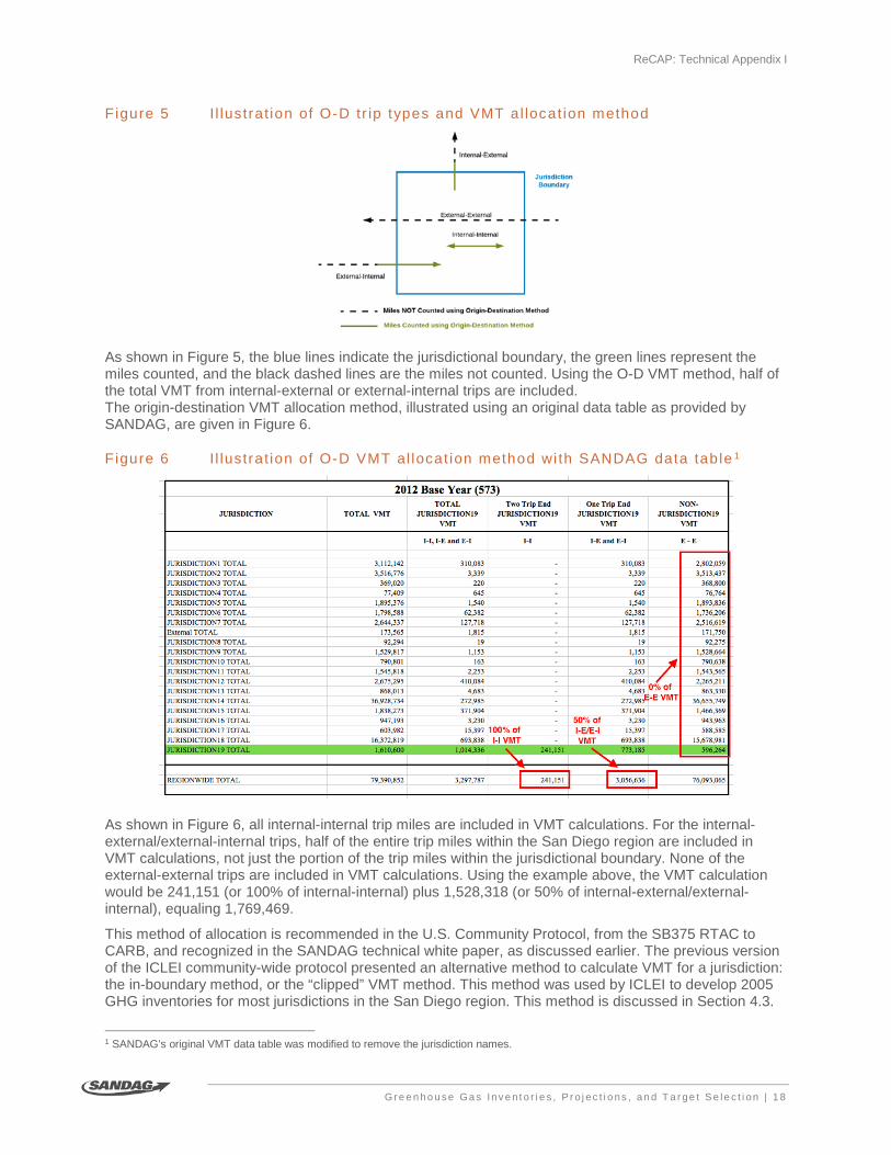
F igure 5 I l lustrat ion of O-D tr ip types and VMT al locat ion method

As shown in Figure 5, the blue lines indicate the jurisdictional boundary, the green lines represent the miles counted, and the black dashed lines are the miles not counted. Using the O-D VMT method, half of the total VMT from internal-external or external-internal trips are included. The origin-destination VMT allocation method, illustrated using an original data table as provided by SANDAG, are given in Figure 6.

Figure 6 I l lustrat ion of O-D VMT al locat ion method wi th SANDAG data table 1

As shown in Figure 6, all internal-internal trip miles are included in VMT calculations. For the internal-external/external-internal trips, half of the entire trip miles within the San Diego region are included in VMT calculations, not just the portion of the trip miles within the jurisdictional boundary. None of the external-external trips are included in VMT calculations. Using the example above, the VMT calculation would be 241,151 (or 100% of internal-internal) plus 1,528,318 (or 50% of internal-external/external-internal), equaling 1,769,469.

This method of allocation is recommended in the U.S. Community Protocol, from the SB375 RTAC to CARB, and recognized in the SANDAG technical white paper, as discussed earlier. The previous version of the ICLEI community-wide protocol presented an alternative method to calculate VMT for a jurisdiction: the in-boundary method, or the “clipped” VMT method. This method was used by ICLEI to develop 2005 GHG inventories for most jurisdictions in the San Diego region. This method is discussed in Section 4.3.

1 SANDAG’s original VMT data table was modified to remove the jurisdiction names.



The SANDAG VMT data are provided in miles per weekday, and the last steps to calculate total VMT for a community are to convert average weekday VMT to average daily VMT, then calculate annual VMT. The weekday to annual conversion factor is based on the conversion factor from average weekday to annual (347 weekdays to 365 days per year) described in the CARB statewide inventory technical support document (CARB, 2016).

The annual VMT is calculated using Equation 4.

Equat ion 4 Annual VMT calculat ion

𝐴𝐴𝐸𝐸𝐸𝐸𝑓𝑓𝑁𝑁𝑓𝑓 𝑉𝑉𝑀𝑀𝑀𝑀 = � (𝑉𝑉𝑀𝑀𝑀𝑀𝑒𝑒𝑒𝑒𝑒𝑒𝑠𝑠 𝑒𝑒𝑒𝑒𝑠𝑠𝑒𝑒 ∗ 𝐴𝐴𝑓𝑓𝑓𝑓𝐸𝐸𝐹𝐹𝑁𝑁𝑁𝑁𝐸𝐸𝐸𝐸𝐸𝐸 𝐸𝐸𝑁𝑁𝐹𝐹𝑁𝑁𝐸𝐸𝑁𝑁𝑒𝑒𝑒𝑒𝑒𝑒𝑠𝑠 𝑒𝑒𝑒𝑒𝑠𝑠𝑒𝑒)𝑒𝑒𝑒𝑒𝑒𝑒𝑠𝑠 𝑒𝑒𝑒𝑒𝑠𝑠𝑒𝑒

∗ 347

Where, Annual VMT = annual VMT of a jurisdiction (miles/year) 𝑉𝑉𝑀𝑀𝑀𝑀𝑒𝑒𝑒𝑒𝑒𝑒𝑠𝑠 𝑒𝑒𝑒𝑒𝑠𝑠𝑒𝑒 = VMT for a given trip type (miles/weekday) 𝐴𝐴𝑓𝑓𝑓𝑓𝐸𝐸𝐹𝐹𝑁𝑁𝑁𝑁𝐸𝐸𝐸𝐸𝐸𝐸 𝐸𝐸𝑁𝑁𝐹𝐹𝑁𝑁𝐸𝐸𝑁𝑁𝑒𝑒𝑒𝑒𝑒𝑒𝑠𝑠 𝑒𝑒𝑒𝑒𝑠𝑠𝑒𝑒 = allocation factor using O-D Method of a given trip type (%) 347 = conversion factor, weekday to annual With, trip type = [Internal-Internal, Internal-External/External-Internal, External-External]

For example, using the VMT by trip type given in Table 10, the 2012 annual VMT for a sample jurisdiction are 614,005,743 miles, as calculated in Equation 5.

Equat ion 5 Example of a jur isd ict ion ’s annual VMT calculat ion

𝐴𝐴𝐸𝐸𝐸𝐸𝑓𝑓𝑁𝑁𝑓𝑓 𝑉𝑉𝑀𝑀𝑀𝑀 = � (𝑉𝑉𝑀𝑀𝑀𝑀𝑒𝑒𝑒𝑒𝑒𝑒𝑠𝑠 𝑒𝑒𝑒𝑒𝑠𝑠𝑒𝑒 ∗ 𝐴𝐴𝑓𝑓𝑓𝑓𝐸𝐸𝐹𝐹𝑁𝑁𝑁𝑁𝐸𝐸𝐸𝐸𝐸𝐸 𝐸𝐸𝑁𝑁𝐹𝐹𝑁𝑁𝐸𝐸𝑁𝑁𝑒𝑒𝑒𝑒𝑒𝑒𝑠𝑠 𝑒𝑒𝑒𝑒𝑠𝑠𝑒𝑒)𝑒𝑒𝑒𝑒𝑒𝑒𝑠𝑠 𝑒𝑒𝑒𝑒𝑠𝑠𝑒𝑒

∗ 347

= �241,151𝐸𝐸𝐸𝐸𝑓𝑓𝑓𝑓𝐸𝐸

𝑤𝑤𝑓𝑓𝑓𝑓𝑤𝑤𝑤𝑤𝑁𝑁𝑤𝑤∗ 100% + 3,056,636

𝐸𝐸𝐸𝐸𝑓𝑓𝑓𝑓𝐸𝐸𝑤𝑤𝑓𝑓𝑓𝑓𝑤𝑤𝑤𝑤𝑁𝑁𝑤𝑤

∗ 50% + 594,264𝐸𝐸𝐸𝐸𝑓𝑓𝑓𝑓𝐸𝐸

𝑤𝑤𝑓𝑓𝑓𝑓𝑤𝑤𝑤𝑤𝑁𝑁𝑤𝑤∗ 0%� ∗ 347

= 614,005,743𝐸𝐸𝐸𝐸𝑓𝑓𝑓𝑓𝐸𝐸𝑤𝑤𝑓𝑓𝑁𝑁𝑁𝑁

3.5.2 Average vehicle emission rate The average vehicle CO2 emission rate is derived from the statewide EMFAC mobile source emissions model developed by CARB and converted to CO2e using a conversion rate derived from the EPA.

EMFAC CO2 emission rate The current version of EMFAC is EMFAC2014, adopted by CARB in 2015. The EMFAC model has undergone methodology and data source updates since its previous versions, EMFAC2007 and EMFAC2011. EMFAC2007 and EMFC2011 are the vehicle emission rate sources for most of the existing GHG inventories used by jurisdictions in the San Diego region.

Table 12 represents the selections used to download emission rates output files from the EMFAC2014 web database. The smallest geographic area selection in the database is the Metropolitan Planning Organization (MPO) or county level; therefore, EPIC uses the emission rate in the San Diego region for all jurisdictions in the region.



Table 12 EMFAC2014 web database (v1.0.7) defaul t mode select ion for emission rate output

Category Selection Data type Emission rates

Region MPO: SANDAG County: San Diego

Calendar year Inventory year Season Annual Vehicle category EMFAC2011 categories (All) Model year Aggregated or all model years Speed Aggregated Fuel All (gas, diesel, electric)

The EMFAC2014 emissions rate output file includes running, start, and idling exhaust emissions rates for the criteria pollutants and CO2. To calculate the average vehicle CO2 emission rate, it is necessary to use the VMT distribution (also provided in the EMFAC output file) and the CO2 running exhaust emission rate (emissions from vehicle tailpipe while traveling on roads) for each type of vehicle category with each fuel type.

CARB released the next model version, EMFAC2017, in December 2017 and is expected to get approval from EPA in 2018. EMFAC2017 includes a GHG module that provides GHG emission estimates directly, including CO2, CH4 and N2O, assuming complete combustion of the fuel (all carbon content of the fuel is converted to CO2) and CH4 and N2O emission rates based on CARB vehicle testing data. No off-model CO2 to CO2e conversion (discussed in the following Section 3.5.2.2) will be needed once EMFAC2017 is approved and used for estimating emissions from on-road transportation.

EPIC is developing a Technical Working Paper, “Estimating a Greenhouse Gas Emission Rate for Miles Driven: A Method for Climate Action Planning,” which will include comparisons of the model versions and more details on estimating the average vehicle emission rate for GHG inventories and projections.

EPA CO2 to CO2e conversion factor On-road transportation also produces CH4 and N2O emissions. EMFAC2014 does not provide CH4 and N2O exhaust emissions. Therefore, the CO2 emission rate is converted to a CO2e emission rate that includes both CH4 and N2O emissions. The conversion factor is based on the EPA GHG Emissions Inventory. The latest EPA GHG Inventory provides CH4 and N2O emissions for fossil fuel combustion in on-road vehicles and off-road equipment. Only the on-road CH4 and N2O emissions are used, and all fuel types (gasoline, diesel, and alternative fuels) are included. The CH4 and N2O emissions are converted to CO2e using the associated GWPs given in Table 4. Sources and methods are updated in each iteration of the U.S. GHG Emission Inventory. The CO2, CH4, and N2O emissions of the same year vary slightly in each updated version. EPIC uses an average of the CO2e to CO2 emissions ratio from the most recent three years as the conversion factor. This conversion factor is currently 1.01.

Table 13 CO2, CH4, and N2O emiss ions f rom on-road mobi le combust ion in U.S. (2012-2014)

Calendar year CO2 emissions (MMT CO2e)

CH4 emissions

(MMT CO2e)

N2O emissions

(MMT CO2e)

Total emissions

(MMT CO2e) CO2e to

CO2 ratio

2012 1,613 1.6 14.5 1,629 1.01 2013 1,628 1.6 14.5 1,645 1.01 2014 1,656 1.4 12.6 1,671 1.01

Average 1.01 MMT – million metric tons Source: EPA 2016



Average vehicle CO2e emission rate for the San Diego region The average vehicle GHG emissions rate, or the combination of the conversion factor and the average vehicle CO2 emission rate, can be calculated in terms of CO2e according to Equation 6.

Equat ion 6 Average vehic le CO2e emission rate calculat ion (San Diego region)

𝐻𝐻𝑂𝑂2𝑓𝑓 𝐸𝐸𝑅𝑅𝑐𝑐𝑎𝑎𝑒𝑒 = � (𝑉𝑉𝑀𝑀𝑀𝑀 𝐷𝐷𝐸𝐸𝐸𝐸𝑁𝑁𝑁𝑁𝑒𝑒𝑐𝑐𝑒𝑒𝑒𝑒𝑐𝑐𝑐𝑐𝑒𝑒𝑒𝑒,𝑓𝑓𝑠𝑠𝑒𝑒𝑒𝑒 ∗ 𝐻𝐻𝑂𝑂2 𝑅𝑅𝑅𝑅𝑁𝑁𝐸𝐸𝑅𝑅𝑒𝑒𝑐𝑐𝑒𝑒𝑒𝑒𝑐𝑐𝑐𝑐𝑒𝑒𝑒𝑒,𝑓𝑓𝑠𝑠𝑒𝑒𝑒𝑒𝑒𝑒𝑒𝑒𝑐𝑐𝑠𝑠𝑠𝑠,𝑓𝑓𝑠𝑠𝑒𝑒𝑒𝑒

) ∗ 1.01

Where,

𝐻𝐻𝑂𝑂2 𝑓𝑓𝐸𝐸𝑅𝑅𝑐𝑐𝑎𝑎𝑒𝑒 = average vehicle CO2 emission rate of all vehicle classes and fuel types in the region (grams CO2e per mile)

𝑉𝑉𝑀𝑀𝑀𝑀 𝐷𝐷𝐸𝐸𝐸𝐸𝑁𝑁𝑁𝑁𝑒𝑒𝑐𝑐𝑒𝑒𝑒𝑒𝑐𝑐𝑐𝑐𝑒𝑒𝑒𝑒 𝑓𝑓𝑠𝑠𝑒𝑒𝑒𝑒 =VMT of a given vehicle class with a given fuel out of total VMT in the San Diego region (%)

𝐻𝐻𝑂𝑂2 𝑅𝑅𝑅𝑅𝑁𝑁𝐸𝐸𝑅𝑅𝑒𝑒𝑐𝑐𝑒𝑒𝑒𝑒𝑐𝑐𝑐𝑐𝑒𝑒𝑒𝑒 𝑓𝑓𝑠𝑠𝑒𝑒𝑒𝑒 = CO2 running exhaust emissions of a given vehicle with a given fuel (grams CO2 per mile)

1.01 = Conversion factor from CO2 to CO2e

With,

𝐻𝐻𝑓𝑓𝑁𝑁𝐸𝐸𝐸𝐸 = [EMFAC2011 Categories, EMFAC2014 Technical Documentation Table 6.1]

𝐸𝐸𝑓𝑓𝑓𝑓𝑓𝑓 = [Gas, Diesel, Electric] Using Equation 6 above, the San Diego region’s average vehicle emission rates from 2012 to 2015 are given in Table 14.

Table 14 Average vehic le emiss ion rate (2012-2015) for the San Diego region

Year Average vehicle emission factor (gram CO2e/mile)

2012 483 2013 476 2014 468 2015 457

Source: CARB, EPIC 2016

3.5.3 Emissions calculation for on-road transportation category Total emissions from the on-road transportation category are estimated by multiplying the average vehicle emission rate in the San Diego region with the jurisdiction’s annual VMT in a given year, as shown in Equation 7.

Equat ion 7 Emission calculat ion for on-road transportat ion category

𝐺𝐺𝐺𝐺𝐺𝐺 𝐸𝐸𝐸𝐸𝐸𝐸𝐸𝐸𝐸𝐸𝐸𝐸𝐸𝐸𝐸𝐸𝐸𝐸𝑒𝑒𝑒𝑒𝑐𝑐𝑡𝑡𝑠𝑠𝑠𝑠 = 𝑁𝑁𝐸𝐸𝐸𝐸𝑓𝑓𝑁𝑁𝑓𝑓 𝑉𝑉𝑀𝑀𝑀𝑀 ∗ 𝐻𝐻𝑂𝑂2𝑓𝑓 𝐸𝐸𝑅𝑅𝑐𝑐𝑎𝑎𝑒𝑒 ∗ 10−6 Where, 𝐺𝐺𝐺𝐺𝐺𝐺 𝐸𝐸𝐸𝐸𝐸𝐸𝐸𝐸𝐸𝐸𝐸𝐸𝐸𝐸𝐸𝐸𝐸𝐸𝑒𝑒𝑒𝑒𝑐𝑐𝑡𝑡𝑠𝑠𝑠𝑠 = emissions from on-road transportation category in a given year

(MT CO2e) 𝑁𝑁𝐸𝐸𝐸𝐸𝑓𝑓𝑁𝑁𝑓𝑓 𝑉𝑉𝑀𝑀𝑀𝑀 = annual VMT of a jurisdiction (miles/year) 𝐻𝐻𝑂𝑂2𝑓𝑓 𝐸𝐸𝑅𝑅𝑐𝑐𝑎𝑎𝑒𝑒 = average vehicle CO2e emission rate of all vehicle classes and fuel

types in the region (grams CO2e per mile) 10−6 = conversion factor, MT per gram CO2e

Using the example of the annual VMT from Equation 5, the annual on-road transportation emissions are 260,127 MT CO2e as calculated in Equation 8.



Equat ion 8 Example of annual on- road transpor tat ion emiss ion calculat ion

𝐺𝐺𝐺𝐺𝐺𝐺 𝐸𝐸𝐸𝐸𝐸𝐸𝐸𝐸𝐸𝐸𝐸𝐸𝐸𝐸𝐸𝐸𝐸𝐸𝑒𝑒𝑒𝑒𝑐𝑐𝑡𝑡𝑠𝑠𝑠𝑠 = 𝑁𝑁𝐸𝐸𝐸𝐸𝑓𝑓𝑁𝑁𝑓𝑓 𝑉𝑉𝑀𝑀𝑀𝑀 ∗ 𝐻𝐻𝑂𝑂2𝑓𝑓 𝐸𝐸𝑅𝑅𝑐𝑐𝑎𝑎𝑒𝑒 ∗ 10−6

= 614,005,743𝐸𝐸𝐸𝐸𝑓𝑓𝑓𝑓𝐸𝐸𝑤𝑤𝑓𝑓𝑁𝑁𝑁𝑁

∗ 483𝑔𝑔 𝐻𝐻𝑂𝑂2𝑓𝑓𝐸𝐸𝐸𝐸𝑓𝑓𝑓𝑓

∗ 10−6𝑀𝑀𝑀𝑀 𝐻𝐻𝑂𝑂2𝑓𝑓𝑔𝑔 𝐻𝐻𝑂𝑂2𝑓𝑓

= 296,565 𝑀𝑀𝑀𝑀 𝐻𝐻𝑂𝑂2𝑓𝑓

3.5.4 Limitations of method used to calculate emissions from on-road transportation

Travel demand model updates As discussed in the activity data collection (Section 3.5.1), SANDAG updates the regional travel demand model for each RTP update approximately every four years.

Due to the model and data sources updates, it is not feasible to re-calibrate VMT data for years prior to a newer version’s base year. For example, for jurisdictions in the region using 2005 or 2010 as the CAP baseline year, the VMT data for the CAP baseline years are from previous versions of the travel demand model. Additionally, due to the model and data sources updates, VMT data cannot be compared across versions for the same year. SANDAG has switched from four-step transportation model to activity-based model starting with Series 13. The projected 2012 VMT data from Series 12 cannot be compared with the 2012 VMT data from Series 13. More discussion on VMT comparison is in Section 4.3.

Use of state model for the San Diego region While the VMT data are specifically tailored to each jurisdiction in the San Diego region, the average vehicle emission rate for the San Diego region is used for all jurisdictions. This value includes the embedded assumptions in the EMFAC model, such as the regional VMT distribution of each vehicle class and alternative-fueled vehicle (AFV) sales in the region. The assumptions in EMFAC may not match the actual conditions in the region or in a particular jurisdiction. For example, if a jurisdiction has more AFV sales, including electric vehicle sales, than the EMFAC model assumptions for the whole region, the regional emission factor may be an overestimate for the jurisdiction.

Additionally, the average vehicle emission rate used in this Appendix is based on the VMT distribution of each vehicle category in the EMFAC model for the San Diego region and the emission factor for each vehicle category. In the EMFAC2011 model, the VMT inputs for the San Diego region were provided by SANDAG to CARB, so that the original source of VMT and emission factor were consistent. In EMFAC2014, the VMT inputs were estimates by CARB based on fuel sale data from the State Board of Equalization, vehicle populations, and odometer data from the Department of Motor Vehicles. Depending on the difference between the models and inputs, the VMT distribution in the EMFAC model may not be consistent with the VMT data in SANDAG’s travel demand model. In addition, VMT data for the San Diego region from versions of the EMFAC model also show differences.

3.6 GHG emissions from the water category

Emissions from water use in a jurisdiction arise from the energy required to move water from origin sources to end-use customers, including upstream supply and conveyance, water treatment, and water distribution, as shown in Figure 7. The energy required to move water is primarily electricity but may include natural gas or other fuels.



F igure 7 Segments of the water cyc le (CEC, 2005)

Method ‘WW.14 Energy-related Emissions Associated with Water Delivery and Treatment’ of the U.S Community Protocol is used to estimate the GHG emissions from water use, with regional or jurisdictionally-specific data sources described in the following sections. Emissions from water end-use, including water heating and cooling at homes and businesses, are included in the electricity and natural gas categories rather than in the water category.

3.6.1 Overview of the water system in the San Diego region The San Diego County Water Authority (SDCWA) is the water wholesaler for the San Diego region. It serves 95% of the population in the San Diego region through its 24 member agencies. Each member agency purchases treated and/or untreated water from SDCWA. The rest of the water supply is from local sources, including surface water, ground water, and recycled water. The service area of a SDCWA member agency may cover part of a jurisdiction, a single jurisdiction, or parts of several jurisdictions in the San Diego region, as shown in Figure 8.



F igure 8 Service area map of SDCW A member agenc ies (SanGIS, EPIC 2015)

Not all SDCWA member agencies have their own water treatment plants (WTPs). Member agencies that do not have WTPs purchase treated water from other member agencies or from SDCWA. For example, both the Cities of San Diego and Del Mar are member agencies of the SDCWA, but the City of San Diego provides water treatment service for the City of Del Mar.

For jurisdictions (or parts of jurisdictions) not covered by SDCWA member agencies, such as the City of Imperial Beach, the City of Coronado, or eastern parts of the unincorporated County of San Diego, water services are provided by private water companies and/or small community water systems. For example, the California American Water Company (CalAM) serves the Cities of Imperial Beach and Coronado with water purchases from the City of San Diego. Eastern parts of the unincorporated County of San Diego are primarily covered by small community water systems and private groundwater wells at residents’ premises.

3.6.2 Activity – water use Potable water Potable water use data for a jurisdiction are provided by a jurisdiction’s public utility department, or by SDCWA member agencies that supply the water for the jurisdiction, upon request. The source of water and where the water is treated are two key factors in the GHG emission calculation for the water category. Therefore, in addition to the water delivered, the water production information for the water agency’s entire service area (amount of water purchased by the member agency from each source) is also requested and collected. Water use data are collected in the following format (Table 15) for the inventory year, with the blank cells to be filled by the jurisdiction or water agency. The frequency and timing of data availability can be different for different water agencies.



Table 15 Example of water use data requests ( for a jur isd ict ion, f rom a SDCW A member agency)

Annual potable water delivery to jurisdiction

Jurisdiction 1 million gallons or acre feet Total water delivered

Annual potable water production of entire service area

Water source million gallons or acre feet SDCWA treated water SDCWA untreated water Local surface water Local ground water

One water agency serving multiple jurisdictions may indicate that it is not possible to separate out customers or water meter locations by jurisdiction in its entire service area. It is also possible that a water agency may not track water delivery data by jurisdiction. In this case, the water production in the entire service area is allocated by the population of each jurisdiction served by the agency.

Recycled water Recycled water or reclaimed water that does not meet drinking water standards can still be used for some agriculture, landscape and golf course irrigation use, or power plant cooling use. Recycled water reduces the demand for potable water. Recycled water is treated at wastewater treatment plants (WWTPs) and/or Water Reclamation Facilities (WRFs) with tertiary or advanced treatment. Examples of these plants in the region are the San Elijo Water Reclamation Facility, which provides recycled water in North San Diego County, and the North City Water Reclamation Plant in City of San Diego. Like potable water data, the recycled water use data are collected in the format shown in Table 16 for the inventory year, with the blank cells to be filled by the jurisdiction or water agency.

Table 16 Example of recycled water use data

Annual recycled water delivery to jurisdiction

Total water delivered (million gallon or acre foot) Recycled water production facility



3.6.3 Energy intensity of water One component of the water emission factor is the energy intensity, or energy needed to move one unit of water through each segment of the water system, expressed in kWh per acre foot (kWh/AF) or kWh/million gallons. Each of the water sources described in the activity data section above goes through different segments of the water system, as shown in Figure 9 below. Therefore, different energy intensities are applied to each water source.

Figure 9 W ater sources and assoc iated segments of the water supply sys tem

The total energy intensity used to calculate GHG emissions from the water category comprises an upstream energy intensity value and a local energy intensity value.

Upstream energy intensity The upstream energy use in Figure 9 refers to the energy needed to move water from the original sources to the SDCWA member agency’s service area, or the first delivery point in the service area. For example, untreated water could be sent to the SDCWA member agency’s reservoir, or treated water could be sent directly to the member agency’s distribution system pipelines.

Water suppliers have begun to voluntarily report the energy intensity in their service areas in an Urban Water Management Plan (UWMP). SDCWA’s and Metropolitan Water District’s (MWD’s) 2015 UWMP voluntary energy intensity reporting is used to calculate the upstream supply energy intensity for SDCWA’s member agencies. The energy intensity based on the average of fiscal years 2013 and 2014 is shown in Table 17.



Table 17 Components of average upstream energy intens i ty for SDCW A member agenc ies

Water system segment FY 2013 and 2014 average energy

intensity (kWh/AF) Data source

MWD delivered untreated* 1,817 MWD UWMP 2015 Appendix 9 SDCWA conveyance** -62 SDCWA UWMP 2015 Appendix K SDCWA untreated subtotal 1,755 SDCWA treatment 60 SDCWA UWMP 2015 Appendix K SDCWA distribution*** 1.1 SDCWA UWMP 2015 Appendix K SDCWA treated total 1,816 *Includes conveyance from the State Water Project & Colorado River water to MWD’s distribution system, and distribution from MWD to MWD’s member agencies **Conveyance of raw water supplies to the water treatment plants or to member agency connections (negative value means hydro-electric generation by SDCWA) *** Distribution of treated water from SDCWA’s Twin Oaks water treatment plant to SDCWA’s member agencies “Upstream” refers to moving water from the original source to SDCWA’s member agency’s service area or first connection point

Local energy intensity Local energy intensity refers to the energy needed to treat and move (or distribute) water within the water agency’s service area. Local energy intensity depends on the water sources, the treatment level, capacity, and efficiency of the associated water treatment plant. For example, brackish groundwater requires advanced treatment, such as reverse osmosis, to remove the salinity in the water, so its treatment has higher energy use than treating surface water with conventional treatment methods. Local distribution energy intensity depends on the service area’s geological conditions, such as the elevation the water is pumped to/from and the pump station’s energy efficiency. For some agencies, the water delivered to the service area is already under pressure and the distribution system is gravity-fed; therefore, no energy is required for local distribution.

Each water agency’s service area conditions are different and limited data are available on local energy intensity. Funded by a grant from The San Diego Foundation, EPIC is currently working with SDCWA member agencies to develop local energy intensity values for up to nine jurisdictions in the San Diego region. The results are expected to be released in mid 2018. The following is an example of a local energy intensity calculation using the City of San Diego’s 2015 UWMP voluntary energy intensity data. The local energy intensity for other agencies in the San Diego region may be considerably different from the City of San Diego’s.

The City of San Diego’s Public Utility Department (SDPUD) manages the City’s water system. In its 2015 UWMP, detailed energy intensities for fiscal year 2015 are reported for each segment of the water system. A local energy intensity value for each water source is determined by combining these energy intensity values with the water source descriptions in Figure 9. Table 18 shows the reported local energy intensities for potable water and Table 19 shows the reported local energy intensities for recycled water.



Table 18 Example of potable water local energy intens i ty (City of San Diego, 2015)

Segment of water system

Energy intensity (KWh/AF, FY 2015)

SDCWA treated

SDCWA untreated

Local surface

Local ground

SDPUD groundwater extraction 279.4

SDPUD placed into storage 55.9

SDPUD conveyance 2.5

SDPUD treatment 24.4

SDPUD distribution 42.8

Total local intensity for each source 43 67 126 349 SDPUD = City of San Diego Public Utilities Department Only the electricity purchased from SDG&E (net energy) is included, on-site renewable generation at water treatment plants is not included. Source: SDPUD Urban Water Management Plan 2015

Table 19 Example of recycled water energy in tens ity (Ci ty of San Diego, 2015)

Segment of water system Energy intensity (kWh/AF, FY 2015)

SDPUD recycled water treatment 0.2 SDPUD recycled water distribution 37.7 Recycled water total 38 SDPUD = City of San Diego Public Utilities Department Recycled water treatment energy intensity (tertiary treatment) is in addition to wastewater treatment. Source: SDPUD Urban Water Management Plan 2015

3.6.4 Electricity emission factor associated with water energy intensity To convert the energy intensity of water (kWh/AF or kWh/million gallons) to GHG emissions per unit of water, the electricity emission factor associated with the energy use is applied. For upstream energy use, a California-wide average emission factor from EPA eGRID is applied. For local energy use, either the SDG&E electricity emission factor or the DA emission factor is applied. The methods to estimate the emission factors are described in Section 3.3.

3.6.5 Emission calculation for water category Based on the water sources, energy intensities, and electricity emission factors, the emissions from the water category are calculated using Equation 9 below.



Equat ion 9 Emission calculat ion for water category

𝐺𝐺𝐺𝐺𝐺𝐺 𝐸𝐸𝐸𝐸𝐸𝐸𝐸𝐸𝐸𝐸𝐸𝐸𝐸𝐸𝐸𝐸𝐸𝐸𝑤𝑤𝑐𝑐𝑒𝑒𝑒𝑒𝑒𝑒 = � (𝐺𝐺𝑠𝑠𝑐𝑐𝑠𝑠𝑒𝑒𝑒𝑒𝑒𝑒 ∗ 𝐸𝐸𝐸𝐸𝑠𝑠𝑐𝑐𝑠𝑠𝑒𝑒𝑒𝑒𝑒𝑒,𝑠𝑠𝑒𝑒𝑐𝑐𝑐𝑐𝑒𝑒𝑡𝑡𝑒𝑒 ∗ 𝐸𝐸𝐸𝐸𝑠𝑠𝑐𝑐𝑠𝑠𝑒𝑒𝑒𝑒𝑒𝑒,𝑠𝑠𝑒𝑒𝑐𝑐𝑐𝑐𝑒𝑒𝑡𝑡𝑒𝑒 ∗ 10−3) ∗ 0.000453𝑠𝑠𝑐𝑐𝑠𝑠𝑒𝑒𝑒𝑒𝑒𝑒,𝑠𝑠𝑒𝑒𝑐𝑐𝑐𝑐𝑒𝑒𝑡𝑡𝑒𝑒

Where, 𝐺𝐺𝐺𝐺𝐺𝐺 𝐸𝐸𝐸𝐸𝐸𝐸𝐸𝐸𝐸𝐸𝐸𝐸𝐸𝐸𝐸𝐸𝐸𝐸𝑤𝑤𝑐𝑐𝑒𝑒𝑒𝑒𝑒𝑒 = emissions from water category in a given year (MT CO2e) 𝐺𝐺𝑠𝑠𝑐𝑐𝑠𝑠𝑒𝑒𝑒𝑒𝑒𝑒 = annual water delivered to a jurisdiction in a given year (acre foot or gallon) 𝐸𝐸𝐸𝐸𝑠𝑠𝑐𝑐𝑠𝑠𝑒𝑒𝑒𝑒𝑒𝑒,𝑠𝑠𝑒𝑒𝑐𝑐𝑐𝑐𝑒𝑒𝑡𝑡𝑒𝑒 = energy intensity of a water source at a segment of the water system

(kWh/acre foot or kWh/gallon) 𝐸𝐸𝐸𝐸𝑠𝑠𝑐𝑐𝑠𝑠𝑒𝑒𝑒𝑒𝑒𝑒,𝑠𝑠𝑒𝑒𝑐𝑐𝑐𝑐𝑒𝑒𝑡𝑡𝑒𝑒 = electricity emission factor of a water source at a segment of the water

system (lbs CO2e/MWh) 10−3 = conversion factor, kWh to MWh 0.000453 = conversion factor, metric tons CO2e in a pound With, source = [SDCWA treated, SDCWA untreated, local surface water, local

groundwater, recycled water] segment = [upstream supply, local conveyance, local treatment, local distribution,

local recycled water treatment, local recycled water distribution]

3.6.6 Method to avoid double-counting emissions related to electricity category For some jurisdictions, the water treatment plants, groundwater extraction wells, and/or recycled water reclamation facilities are within the jurisdictional boundary; therefore, the electricity and emissions associated with those facilities are already included in the electricity category. For example, the Escondido-Vista Water Treatment Plant (WTP) that treats purchased raw water from SDCWA for the City of Escondido and Vista Irrigation District is located in the City of Escondido. The electricity used at this plant is part of the electricity use in Escondido. To avoid double counting, the electricity use and associated emissions at the Escondido–Vista WTP to treat potable water for the City of Escondido is removed from the electricity category. For example, if half of the water treated at the Escondido-Vista WTP were for the City of Escondido’s customers, 50% of the electricity use at the plant would be removed from Escondido’s GHG inventory electricity category.

Similarly, all local distribution electricity use and emissions are captured in the electricity category. As these emissions are included in the water category they must be subtracted from the electricity category.

The following process (Table 20) is used to determine the amount of electricity and associated emissions that must be subtracted from the electricity category. This process describes each water source, segment, and facility that is considered.



Table 20 Process to avoid double-count ing water- re lated emissions assoc iated wi th the e lectr ic i t y category

Potable water

Is the water treatment plant within the jurisdictional boundary? Y/N Is SDCWA raw water treated in-boundary? Y/N % SDCWA raw water treated in-boundary 0-100% Is the surface water treated in-boundary? Y/N % surface water treated in-boundary 0-100% Is the groundwater extracted in-boundary? Y/N % groundwater extracted in-boundary 0-100% Is the groundwater treated? Y/N % groundwater undergoing treatment? 0-100% Is the groundwater treated in-boundary? Y/N % groundwater treated in-boundary? 0-100%

Recycled water

Is the recycled water treated at WWTPs in-boundary? Y/N % recycled water from WWTP in-boundary? 0-100%

3.6.7 Limitations of method used to calculate emissions from water One water agency serving multiple jurisdictions As discussed in the data collection section, it can be difficult to determine water delivery by jurisdiction if one water agency serves several jurisdictions. Agencies may track water pumping energy use at different pressure zones that serve different jurisdictions, and they may use the percentage of energy allocated for this purpose to assign water delivery amounts. Sometimes, one water agency serving multiple jurisdictions may not be able to separate out customers or water meter locations by jurisdiction for its entire service area. They may also not track water delivery data by jurisdiction. In this case, water production in the entire service area may be allocated by population for each jurisdiction served by the agency. However, allocating water use by population may not be representative for certain jurisdictions. This is because per capita water use can vary considerably. For example, if the jurisdiction is agriculture-heavy, using a per capita value may under-represent the jurisdiction’s water use.

Emission factor calculation Unlike the energy or on-road transportation category, limited data are available on energy intensity for the water category. In the past, the CEC’s embedded energy in water studies were used to estimate upstream water emissions. These studies included an estimate for Southern California upstream supply and conveyance energy intensity of 3,169 kWh/AF or 9,727 kWh/million gallons (CEC, 2005) much higher than the 2013-2014 data from SDCWA and MWD UWMPs (see Table 17 above). The energy intensity factor depends on the water source mix (the percentage of water production from each source), which varies widely depending on weather and climate conditions. The average of 2013 and 2014 energy intensities may not be representative for other years. Additionally, at the end of 2015, the Carlsbad Desalination Plant began providing water as part of SDCWA’s treated water supply. Desalination is an energy-intensive water treatment process and not included in the 2013 and 2014 average energy intensity in SDCWA’S UWMP. This may result in higher energy intensity and emissions from the water category in inventories for 2015 and beyond.



3.7 GHG emissions from the wastewater category

Unlike the water category, in which the GHG emissions are from the energy used to move and treat water, the wastewater-related GHG emissions include “process, stationary and fugitive GHG emissions,” as described in U.S Community Protocol ‘WW.1 – WW.14.’

The following sections provide an overview of the wastewater collection system in the San Diego region and describes the methods used to collect wastewater generation data and calculate GHG emissions from wastewater.

3.7.1 Overview of the wastewater collection system in the San Diego region In the San Diego region, most wastewater from end-use is collected by different agencies, conveyed to centralized wastewater treatment plants (WWTPs) or water reclamation facilities (WRFs), and discharged as shown in Figure 10.

Figure 10 W ater and wastewater sys tem (CEC, 2005)

The following are examples of the collecting agencies in the San Diego region that manage the wastewater collection system, including pipelines and pump stations (Figure 11).

Figure 11 Types of wastewater col lec t ion agenc ies in the San Diego region



The Program Environmental Impact Report (PEIR) for San Diego Forward: The Regional Plan (Regional Plan EIR) includes a list of wastewater collection agencies and their collection systems (SANDAG, 2015). Similar to the relationship between jurisdictions and water delivery agencies, one wastewater collection agency may cover all or part of one, or more than one jurisdiction. For the SDCWA member agencies that provide both water and wastewater services, the service areas may be different. For example, Vallecito Water District’s wastewater service area is smaller than its water service area.

Some collecting agencies own and operate one or multiple WWTPs or WRFs, as do most of the collecting agencies in the eastern San Diego region. For example, Valley Center Municipal Water District (Valley Center MWD) collects wastewater in the Hidden Meadows and Valley Center communities of the unincorporated County of San Diego. The wastewater collected is treated at the Valley Center MWD-owned Lower Canyon Moosa WRF and Woods Valley Ranch WRF (Valley Center MWD, 2016). The Regional Plan EIR also includes a list of wastewater agencies that have wastewater treatment facilities. There are a total of 32 existing and planned wastewater treatment facilities, including those with recycled water treatment capability (SANDAG, 2015).

Agencies that do not have treatment facilities convey the wastewater to other centralized WWTPs or WRFs. For example, the City of San Diego operates the Metropolitan Sewerage System, which includes one WWTP (Point Loma WWTP) and two WRFs (North City WRF and South Bay WRF) that provide wastewater treatment, discharge, and recycled water services for the City of San Diego and 15 other cities and collecting agencies. Similarly, the Encina Wastewater Authority and San Elijo Joint Powers Authority provide wastewater treatment, discharge, and recycling water services for the jurisdictions and collecting agencies in the northern San Diego region. The service areas covered by the Metropolitan Sewerage System and Encina Wastewater Authority are shown in Figure 12 as examples.

Figure 12 Service area of San Diego Metropol i tan Sewerage System and Enc ina Wastewater Author i ty

Not all areas in the San Diego region are covered by a centralized wastewater collection and treatment system. In some rural areas in the San Diego region, wastewater treatment occurs through on-site septic systems.



3.7.2 Activity – wastewater generation Wastewater generation for a specific jurisdiction is requested from the collecting agency to identify wastewater amount collected, treatment facility type, and treatment process for each of the wastewater collection facilities. Table 21 is an example data request form for a collecting agency on behalf of a jurisdiction, with the blank cells to be filled by the agency.

Table 21 Example of wastewater data request ( for a jur isd ic t ion, f rom a col lec t ing agency)

Collecting agency 1

Total wastewater collected from Jurisdiction 1 (average MGD – million gallons per day, or million gallon/year) Total population served in Jurisdiction 1: Name of wastewater treatment facility: Treatment process (primary, secondary, tertiary): Does the facility have Anaerobic Digester?

3.7.3 Wastewater emission factor The wastewater emission factor depends on the treatment processes. Treatment levels and processes vary by WWTP. A centralized, conventional WWTP or WRF includes aerobic systems to degrade dissolved organics. Additional treatment includes nitrification/denitrification to oxidize or remove nitrogenous waste, anaerobic digestion to degrade organics to produce digester gas, and combustion of digester gas. A decentralized wastewater treatment system, such as a septic system, only includes physical settling and biological activities without other processes typically used at a centralized WWTP or WRF.

Wastewater emission factor at conventional WWTP or WRF with anaerobic digestion This section describes the stationary emissions from the combustion of digester gas, following method ‘WW.1 – WW.3 Stationary CH4, N2O and CO2 Emissions from Combustion of Digester Gas’ of the U.S Community Protocol. In general, conventional WWTPs have secondary treatment, while some WRFs have tertiary treatment that treats wastewater to recycled water level standards. Point Loma WWTP, the largest WWTP in the San Diego region with a capacity of 240 million gallons per day (MGD), has only primary treatment. It is operated by City of San Diego but treats wastewater from ten jurisdictions and three wastewater agencies in the San Diego region. Point Loma WWTP has anaerobic digesters that capture digester gas to run an on-site co-generation system to produce renewable electricity for the facility and send excess electricity to the grid. The emission factor at Point Loma WWTP is calculated using Equation 10 below.

Equat ion 10 Emission fac tor ca lculat ion for Point Loma WWTP

𝐸𝐸𝐸𝐸𝑠𝑠𝑐𝑐𝑒𝑒𝑡𝑡𝑒𝑒 𝑒𝑒𝑐𝑐𝑐𝑐𝑐𝑐 𝑊𝑊𝑊𝑊𝑊𝑊𝑊𝑊 =𝐺𝐺𝐺𝐺𝐺𝐺 𝐸𝐸𝐸𝐸𝐸𝐸𝐸𝐸𝐸𝐸𝐸𝐸𝐸𝐸𝐸𝐸𝐸𝐸𝑠𝑠𝑐𝑐𝑒𝑒𝑡𝑡𝑒𝑒 𝑒𝑒𝑐𝑐𝑐𝑐𝑐𝑐 𝑊𝑊𝑊𝑊𝑊𝑊𝑊𝑊

𝐺𝐺𝑁𝑁𝐸𝐸𝑁𝑁𝑓𝑓𝑤𝑤𝑁𝑁𝑁𝑁𝑓𝑓𝑁𝑁 𝐸𝐸𝑓𝑓𝐸𝐸𝑤𝑤𝑠𝑠𝑐𝑐𝑒𝑒𝑡𝑡𝑒𝑒 𝑒𝑒𝑐𝑐𝑐𝑐𝑐𝑐 𝑊𝑊𝑊𝑊𝑊𝑊𝑊𝑊

Where 𝐸𝐸𝐸𝐸𝑠𝑠𝑐𝑐𝑒𝑒𝑡𝑡𝑒𝑒 𝑒𝑒𝑐𝑐𝑐𝑐𝑐𝑐 𝑊𝑊𝑊𝑊𝑊𝑊𝑊𝑊 = emission factor at Point Loma WWTP in a given year

(MT CO2e/million gallon) 𝐺𝐺𝐺𝐺𝐺𝐺 𝐸𝐸𝐸𝐸𝐸𝐸𝐸𝐸𝐸𝐸𝐸𝐸𝐸𝐸𝐸𝐸𝐸𝐸𝑠𝑠𝑐𝑐𝑒𝑒𝑡𝑡𝑒𝑒 𝑒𝑒𝑐𝑐𝑐𝑐𝑐𝑐 𝑊𝑊𝑊𝑊𝑊𝑊𝑊𝑊 = Total GHG emissions from Point Loma WWTP, in MT CO2e,

based on facility’s annual CARB mandatory GHG reporting 𝐺𝐺𝑁𝑁𝐸𝐸𝑁𝑁𝑓𝑓𝑤𝑤𝑁𝑁𝑁𝑁𝑓𝑓𝑁𝑁 𝐸𝐸𝑓𝑓𝐸𝐸𝑤𝑤𝑠𝑠𝑐𝑐𝑒𝑒𝑡𝑡𝑒𝑒 𝑒𝑒𝑐𝑐𝑐𝑐𝑐𝑐 𝑊𝑊𝑊𝑊𝑊𝑊𝑊𝑊 = Total wastewater treated at Point Loma WWTP, in million

gallons, based on facility’s annual report



The Point Loma WWTP emission factor comprises the following three emissions components:

• Direct CO2 from combustion of anaerobic digester gas

• CH4 and N2O emissions from digester gas combustion

• Operational fossil fuel emissions from complete combustion

The direct CO2 from combustion of anaerobic digester gas is considered biogenic, while the other two components of CO2 emissions are considered non-biogenic emissions. In 2015, 99% of the GHG emissions from the Point Loma WWTP were biogenic based on its CARB Regulation for the Mandatory Reporting of GHG Emissions (MRR). Biogenic CO2 is part of the short-term carbon cycle and reported separately from the GHG inventory in the statewide inventory. Using Equation 10, the emission factors from 2010 to 2015 are given in Table 22.

Table 22 W astewater emiss ion factors at Point Loma WWTP (2010-2015)

Year Flow

(million gallons/year)

Total emissions (metric tons CO2e – non-biogenic and

biogenic)

Emission factor (MT CO2e/million

gallon)

2010 57,165 75,083 1.31 2011 56,852 21,360 0.38 2012 54,157 22,178 0.41 2013 52,470 20,045 0.38 2014 50,815 22,888 0.45 2015 48,034 21,092 0.44

The MRR reporting method changed after 2010, which is the reason for the lower emission factors after 2010. The change is not due to technology changes at the facility Source: CARB, City of San Diego, EPIC 2017

For other WWTPs or WRFs that have secondary treatment with anaerobic digestion, limited data are available on the emissions from digester gas combustion. The 2013 emission factor for the Encina Wastewater Pollution Control Facility (Encina WPCF) of 1.37 MT CO2e/million gallons (with 11,359 MT CO2e from 8,317 million gallons wastewater treated) is used as a proxy for other WWTPs with similar treatment processes (Encina WPCF, personal communication, 2015).

Wastewater emission factor at conventional WWTP or WRF without anaerobic digestion For centralized WWTPs or WRFs with no anaerobic digesters and only aerobic processes, process emissions are estimated based on ‘WW.7 Process N2O Emission with Nitrification/Denitrification’ or ‘WW.8 Process N2O Emission without Nitrification/Denitrification,’ fugitive emissions are estimated based on ‘WW.12 N2O emissions from effluent discharge’ from the U.S. Community Protocol. Population served by the treatment facilities and the average nitrogen per person (grams N2O/person equivalent) are needed to estimate the emissions. The calculation methods are described in Equation 12.

Many of the WWTPs or WRFs without anaerobic digestion are located in and serving communities in the unincorporated County of San Diego. Limited information is available on the specific treatment processes of these wastewater treatment facilities. One source of this information is from the facilities’ inspection reports that are submitted to the California Regional Water Quality Control Board (CRWQCB). The reports can be requested from the CRWQCB.



Wastewater emission factor from septic systems For emissions from septic systems, the emission factor is based on ‘WW.11 Methane Emissions from Septic Systems’ from the U.S. Community Protocol using a septic system CH4 emission factor (10.7 g CH4/person/day).

Septic systems are primarily in remote areas of the San Diego region, including parts of the unincorporated County of San Diego and cities of Poway, Vista, and San Marcos. The number of people or households that are on septic systems (not connected to municipal wastewater collection systems) are requested from and provided by jurisdiction staff.

3.7.4 Emissions calculation for wastewater category Emissions from the wastewater category are estimated using Equation 11 below, if the emission factor at the wastewater treatment facility is known (as is for Point Loma WWTP and Encina WPCF); if not, Equation 12 is used.

Equat ion 11 Emission calculat ion for wastewater category (where the emission fac tor at the wastewater treatment faci l i t y is known)

𝐺𝐺𝐺𝐺𝐺𝐺 𝐸𝐸𝐸𝐸𝐸𝐸𝐸𝐸𝐸𝐸𝐸𝐸𝐸𝐸𝐸𝐸𝐸𝐸𝑤𝑤𝑐𝑐𝑠𝑠𝑒𝑒𝑒𝑒𝑐𝑐𝑒𝑒𝑒𝑒𝑒𝑒 = � (𝐺𝐺𝐺𝐺𝑐𝑐𝑐𝑐𝑒𝑒𝑡𝑡𝑒𝑒𝑒𝑒 ∗ 𝐸𝐸𝐸𝐸𝑐𝑐𝑐𝑐𝑒𝑒𝑡𝑡𝑒𝑒𝑒𝑒,𝑓𝑓𝑐𝑐𝑒𝑒𝑒𝑒𝑒𝑒𝑒𝑒𝑒𝑒𝑒𝑒)𝑐𝑐𝑐𝑐𝑒𝑒𝑡𝑡𝑒𝑒𝑒𝑒,𝑓𝑓𝑐𝑐𝑒𝑒𝑒𝑒𝑒𝑒𝑒𝑒𝑒𝑒𝑒𝑒

Where, 𝐺𝐺𝐺𝐺𝐺𝐺 𝐸𝐸𝐸𝐸𝐸𝐸𝐸𝐸𝐸𝐸𝐸𝐸𝐸𝐸𝐸𝐸𝐸𝐸𝑤𝑤𝑐𝑐𝑠𝑠𝑒𝑒𝑒𝑒𝑤𝑤𝑐𝑐𝑒𝑒𝑒𝑒𝑒𝑒 = emissions from wastewater category in a given year (MT CO2e) 𝐺𝐺𝐺𝐺𝑐𝑐𝑐𝑐𝑒𝑒𝑡𝑡𝑒𝑒𝑒𝑒 = wastewater collected by a collecting agency from a jurisdiction (gallons

per year, million gallons per year, average million gallons per day) 𝐸𝐸𝐸𝐸𝑐𝑐𝑐𝑐𝑒𝑒𝑡𝑡𝑒𝑒𝑒𝑒,𝑓𝑓𝑐𝑐𝑒𝑒𝑒𝑒𝑒𝑒𝑒𝑒𝑒𝑒𝑒𝑒 = wastewater emission factor at treatment facility (MT CO2e/million gallons) With, agency = each of the wastewater collection agencies facility = [Point Loma WWTP, Encina WPCF], Encina WPCF as proxy for other

wastewater treatment facilities with secondary treatment process and anaerobic digestion

Equat ion 12 Emission calculat ion for wastewater category (where the emission fac tor at the wastewater treatment faci l i t y is unknown)

𝐺𝐺𝐺𝐺𝐺𝐺 𝐸𝐸𝐸𝐸𝐸𝐸𝐸𝐸𝐸𝐸𝐸𝐸𝐸𝐸𝐸𝐸𝐸𝐸𝑤𝑤𝑐𝑐𝑠𝑠𝑒𝑒𝑒𝑒𝑐𝑐𝑒𝑒𝑒𝑒𝑒𝑒 = � (𝐺𝐺𝑠𝑠𝑒𝑒𝑐𝑐𝑒𝑒𝑒𝑒𝑠𝑠𝑠𝑠 ∗ 𝐸𝐸𝐸𝐸𝑁𝑁𝐺𝐺𝑁𝑁,𝑠𝑠𝑒𝑒𝑐𝑐𝑒𝑒𝑒𝑒𝑠𝑠𝑠𝑠 ∗ 𝐺𝐺𝐺𝐺𝐺𝐺𝑁𝑁𝐺𝐺𝑁𝑁)𝑁𝑁𝐺𝐺𝑁𝑁,𝑠𝑠𝑒𝑒𝑐𝑐𝑒𝑒𝑒𝑒𝑠𝑠𝑠𝑠

∗ 10−6

Where, 𝐺𝐺𝐺𝐺𝐺𝐺 𝐸𝐸𝐸𝐸𝐸𝐸𝐸𝐸𝐸𝐸𝐸𝐸𝐸𝐸𝐸𝐸𝐸𝐸𝑤𝑤𝑐𝑐𝑠𝑠𝑒𝑒𝑒𝑒𝑤𝑤𝑐𝑐𝑒𝑒𝑒𝑒𝑒𝑒 = emissions from wastewater category in a given year (MT CO2e) 𝐺𝐺𝑠𝑠𝑒𝑒𝑐𝑐𝑒𝑒𝑒𝑒𝑠𝑠𝑠𝑠 = population served with each of the wastewater treatment process

𝐸𝐸𝐸𝐸𝑁𝑁𝐺𝐺𝑁𝑁,𝑠𝑠𝑒𝑒𝑐𝑐𝑒𝑒𝑒𝑒𝑠𝑠𝑠𝑠 = process emissions per person equivalent (average per person) of a given GHG (grams/person equivalent/year)

𝐺𝐺𝐺𝐺𝐺𝐺𝑁𝑁𝐺𝐺𝑁𝑁 = Global Warming Potential of a given GHG (no units) 10−6 = conversion factor, metric tons CO2e in a gram With, process = [with nitrification/denitrification, without nitrification/denitrification, septic

system] GHG = [CH4, N2O]



3.7.5 Limitations of method used to calculate emissions from wastewater One collecting agency serving multiple jurisdictions If one or more collecting agencies serve several jurisdictions, it is difficult to break out wastewater generation by jurisdiction. If wastewater data cannot be separated, EPIC allocates the wastewater generated in the entire service area by population in each jurisdiction served by the agency. Allocating emissions by population may not be representative in certain jurisdictions. For example, within a collecting agency’s service area, one jurisdiction may have higher outdoor water use than the other jurisdiction, and allocation by per capita may result in over-estimating wastewater generation in one jurisdiction, as outdoor water use does not undergo wastewater treatment.

Emission factor calculation To date, detailed process data is available only for the Encina WPRF. Such data are currently not available for the other wastewater treatment plants in the region, several wastewater agencies have similar processes as Encina and until facility-specific data is available, the emission factor for the Encina WPRF is used as a substitute for all WWTPs or WRFs with anaerobic digestion other than Point Loma WWTP. Because the same treatment processes may have different GHG emissions due to different facility capacities, years of operation, or equipment, the emission factor from the Encina WPRF may not be representative for other facilities in the region. Additionally, this category does not include the emissions associated with energy use at wastewater pump stations and at wastewater treatment facilities. Similar energy intensity calculations for wastewater treatment and collection can be made in this category and separated from the electricity category; however, limited data are available and WWTPs using digester gas as an on-site generation fuel source adds another layer of complexity in this calculation.

3.8 GHG emissions from the solid waste category

GHG emissions from the decomposition of organic material in waste disposed at landfills are broken down into two parts in the U.S. Community Protocol: 1) Method SW.4: methane emissions from community-generated mixed waste in inventory year (waste generated); and 2) Method SW.1: methane emissions from biodegradable waste that has been in place at landfills located within the community boundary (waste in place) (Figure 13).

Figure 13 Types of GHG emissions f rom sol id waste

Only the community-generated waste in the inventory year is accounted for as one of the five basic emission-generating activities, which is the focus of this Appendix. The methodology estimates emissions from all waste disposed by a jurisdiction, regardless of whether the landfills accepting the waste are located inside or outside the jurisdiction boundary. The emissions from waste-in-place at in-boundary landfills are included in the 2012 regional inventory and in the unincorporated County of San Diego CAP baseline inventory.



3.8.1 Activity – waste disposal The California Department of Resources Recycling and Recovery (CalRecycle) Disposal Reporting System (DRS) provides annual waste data. This report includes waste disposed by a jurisdiction, as reported by county and regional agency disposal reporting coordinators. The annual report gives a snapshot of the total amount of waste disposed and where the waste was disposed for a jurisdiction in a given year. Table 23 gives an example of waste disposal by facility for a jurisdiction in the San Diego region. In this example, almost all the waste generated in the jurisdiction was disposed in Otay Landfill and Sycamore Landfill, neither of which are within this jurisdiction’s boundary.

Table 23 Example of a jur isd ict ion ’s waste d isposal by fac i l i t y

Destination facility Waste (tons)

Azusa Land Reclamation Co. Landfill 64 El Sobrante Landfill 49 Otay Landfill 31,033 Sycamore Landfill 33,403 West Miramar Sanitary Landfill 215

Total 67,764

Source: CalRecycle 2017

The amount of waste disposed provided by CalRecycle is verified with the jurisdiction to ensure that no modifications or revisions were made after the jurisdiction submitted the data.

The waste disposal data for the previous calendar year are available in June of the current calendar year.

3.8.2 Solid waste emission factor In previous years, regional inventories have used the default mixed waste emission factor from the U.S Community Protocol Table SW.5, of 0.06 MT CH4/short ton of waste disposed. In recent years, some jurisdictions in the San Diego region have conducted waste characterization studies which provide better data to determine an appropriate and locally-relevant waste emission factor.

A waste characterization study shows the percentage of each waste type in a waste stream disposed in landfills. The study can be for a jurisdiction, such as the City of San Diego’s 2012-2013 Waste Characterization Study, or for a business group or a customer sector, such as CalReycle’s 2014 Statewide Disposal-Facility-Based Characterization. Results of such studies generally classify disposed waste streams into commercial, residential, and self-hauled sectors.

For a jurisdiction with a recent waste characterization study, the jurisdiction-specific mixed waste emission factor may be used. For others, the statewide waste characterization is available. Using a waste characterization study, the mixed waste emission factor can be estimated using the emission rate (MT CH4/short ton or MT CO2e/short ton) of each waste component from the EPA Waste Reduction Model (WARM) and the percentage of the waste component in the waste stream.

EPA WARM is a life-cycle GHG model to assess and compare waste management options (e.g., landfilling, recycling, source reduction, composting), through the life-cycle of waste materials (from material extraction to disposal). However, the GHG inventory method described here does not use a life-cycle approach. In the solid waste category, only emissions from the disposal and associated degradation of waste is included. Therefore, only the landfill emission factors in EPA WARM are used in the calculation. The U.S. Community Protocol recommends using emission factors for each solid waste component from the 2006 (Version 8) of EPA WARM; however, several updates to WARM have been completed since 2006. The methodology described in this Appendix uses the landfill emission factor from the most recent WARM Version 14 (March 2016).



WARM Version 14 reports the landfill CH4 emission factor of each waste material in MT CO2e/short ton, with and without Landfill Gas (LFG) recovery. Because the LFG recovery systems at landfills are different, the emission factor without LFG recovery is used and the default LFG capture rate is incorporated later in the total emission calculation. The mixed waste emission factor is calculated using Equation 13, based on U.S. Community Protocol Equation SW.4.1.

Equat ion 13 Mixed waste emission factor calculat ion

𝐸𝐸𝐸𝐸𝑐𝑐𝑠𝑠𝑤𝑤 = � 𝐺𝐺𝑒𝑒𝑐𝑐𝑐𝑐𝑠𝑠𝑐𝑐𝑡𝑡𝑒𝑒𝑡𝑡𝑒𝑒 ∗ 𝐸𝐸𝐸𝐸𝑒𝑒𝑐𝑐𝑐𝑐𝑠𝑠𝑐𝑐𝑡𝑡𝑒𝑒𝑡𝑡𝑒𝑒𝑒𝑒𝑐𝑐𝑐𝑐𝑠𝑠𝑐𝑐𝑡𝑡𝑒𝑒𝑡𝑡𝑒𝑒

Where: 𝐸𝐸𝐸𝐸𝑐𝑐𝑠𝑠𝑤𝑤 = mixed waste emission factor (MT CO2e/short ton) 𝐺𝐺𝑒𝑒 = distribution of waste components in the mixed waste stream (%) 𝐸𝐸𝐸𝐸𝑒𝑒 = landfill CH4 emission factor without LFG recovery of each waste component from EPA WARM

(MT CO2e/short ton) With,

𝐹𝐹𝐸𝐸𝐸𝐸𝑐𝑐𝐸𝐸𝐸𝐸𝑓𝑓𝐸𝐸𝑁𝑁 = waste component [Paper, Organics, Mixed Residue, etc.] An example of the mixed waste emission factor calculation is given in Table 24, using the City of San Diego’s 2012-2013 Waste Characterization Study. The mixed waste emission factor for the waste disposed by City of San Diego during the study period was 0.744 MT CO2e/short ton.

Table 24 Example of mixed waste emiss ion factor ca lcu lat ion (Ci ty of San Diego, 2012-2013)

Waste component Waste

distribution (%)

Landfill CH4 without LFG Recovery

(MT CO2e/short ton) Paper 16.8% -

Corrugated containers/cardboard 5.0% 2.36 Newspaper 0.8% 0.95

Magazine 0.6% 1.08 Mixed paper (general) 10.4% 2.14

Plastic 8.9% - Glass 1.7% - Metal 3.5% - Organics 38.9% -

Food 15% 1.57 Tree 5.3% 0.77

Leaves and grass 6.8% 0.59 Trimmings 3.5% 0.59

Mixed organics 8.3% 0.53 Electronics 0.6% - C&D 24.6% - Household hazardous waste 0.2% - Special waste 3.1% - Mixed residue 1.6% 0.53 Mixed waste emission factor 0.744 Source: City of San Diego 2014, EPA WARM 2016, EPIC 2016



3.8.3 Landfill gas capture rate EPA WARM assesses three types of landfills: 1) landfills that do not recover LFG, 2) landfills that collect the LFG and flare it without recovering the flare energy, and 3) landfills that collect LFG and combust it for energy recovery by generating electricity. The waste generated by jurisdictions in the San Diego region is disposed at different landfills, and each landfill has a different LFG recovery system. To account for this, the method described here applies the default LFG Collection Efficiency of 75% to all waste disposed, as recommended in the U.S Community Protocol, if no other data is available. However, collection efficiency data should be collected from facility operators if possible. Table 25 shows the estimated LFG collection system efficiencies at the major active landfills in the San Diego region.

Table 25 Major ac t ive landf i l ls in the San Diego region

Landfill name Open/potential close year

Landfill owner/operator

Estimated gas collection system

efficiency Location

Las Pulgas Landfill 1972/2058 Camp Pendleton No collection system Camp Pendleton

Otay Landfill 1963/2033 Republic Services 75% Unincorporated County of San Diego

Sycamore Landfill 1962/2023 Republic Services 75% Santee West Miramar Sanitary Landfill 1983/2022 City of San Diego 69% (provided

by the City) San Diego

Source: EPA MRR Reporting, 2016. EPA SD Landfill Database. EPIC 2017

3.8.4 Emissions calculation for solid waste category Total emissions from the waste disposed in landfills by a jurisdiction is estimated using Equation 14, based on U.S. Community Protocol Equation SW.4.1.

Equat ion 14 Emission calculat ion for so l id waste

𝐺𝐺𝐺𝐺𝐺𝐺 𝐸𝐸𝐸𝐸𝐸𝐸𝐸𝐸𝐸𝐸𝐸𝐸𝐸𝐸𝐸𝐸𝐸𝐸𝑤𝑤𝑐𝑐𝑠𝑠𝑒𝑒𝑒𝑒 = 𝑆𝑆𝐺𝐺 ∗ 𝐸𝐸𝐸𝐸𝑐𝑐𝑠𝑠𝑤𝑤 ∗ (1 − 0.75) ∗ (1 − 0.1) Where: 𝐺𝐺𝐺𝐺𝐺𝐺 𝐸𝐸𝐸𝐸𝐸𝐸𝐸𝐸𝐸𝐸𝐸𝐸𝐸𝐸𝐸𝐸𝐸𝐸𝑤𝑤𝑐𝑐𝑠𝑠𝑒𝑒𝑒𝑒 = emissions from solid waste category in a given year (MT CO2e) 𝑆𝑆𝐺𝐺 = total waste disposal from a jurisdiction (short tons) 𝐸𝐸𝐸𝐸𝑐𝑐𝑠𝑠𝑤𝑤 = mixed waste emission factor (MT CO2e/short ton) 0.75 = default landfill gas capture rate, U.S. Community Protocol, unless otherwise

known 0.1 = default oxidation rate, U.S. Community Protocol

3.8.5 Limitations of method used to calculate emissions from solid waste The delayed release of solid waste emissions The solid waste emissions category is unique because the emissions do not represent the direct emissions in the inventory year, but represent the lifetime emissions from the waste disposed in the inventory year. Unlike other categories discussed in this Appendix, such as burning fuel to produce electricity or operate vehicles, decomposition of organic waste is not an immediate release of emissions.



Recycling and composting The impacts of recycling and composting diversion programs on emissions are partially captured in the inventory. Recycling and diversion programs reduce the amount of community-generated waste sent to the landfills, and this impact is reflected in the waste disposal data. However, the whole life-cycle impact of recycling and composting diversion programs, such as reduction of upstream raw material use and reduced energy use for material processes, are not included in the GHG emissions inventory.

Waste characterization studies The solid waste composition is different in each jurisdiction. Differences exist between residential or commercial sectors, or even between single-family and multi-family buildings. The City of San Diego’s 2012-2013 waste composition study is the most recent and comprehensive study at a jurisdictional level in the region. While this study may represent a more locally-relevant option than statewide data, it may not be representative of all jurisdictions. Nonetheless, it is used to estimate emissions from the solid waste category. As more studies are completed in the region, a more representative regional value can be developed. For example, the City of Oceanside is currently conducting a waste characterization study.

4. Challenges of developing GHG inventories

This section discusses the challenges of developing a communitywide GHG inventory at the jurisdictional level in the San Diego region, including boundary issues, comparability of the activity-based approach with other GHG reporting protocols, and revising and updating previous GHG inventories.

4.1 Boundary issue

A general premise of GHG accounting is to include all emissions within the authority and jurisdiction of a local government. The CARB’s 2017 Climate Change Scoping Plan (2017 Scoping Plan, more discussion in Section 6.2.2) recommends that “plans should disclose all emissions within the defined geographical boundary, even those over which the local government has no regulatory authority to control, and then focus (on) the strategies on those emissions that the jurisdiction controls” (CARB, 2017a, p.100).

However, jurisdictions may not be able to control emissions from some entities within their geographical boundaries. In this case, CAP strategies may or may not affect the activities at these entities that result in GHG emissions. In the San Diego region, the following are examples of such entities:

• Military land – The military has a significant presence in the San Diego region. Military land can span more than one local jurisdiction boundary. For example, Camp Pendleton, adjacent to the City of Oceanside, is located in the unincorporated County of San Diego, and there are Naval bases in the Cities of Coronado and San Diego.

• Native American reservations – San Diego County has 19 tribal reservations within its boundaries. Like military land, these reservations are not subject to local land use and other authority.

• Other agencies – The Port of San Diego and the San Diego County Regional Airport Authority are examples of other agencies that are not subject to the land use authority of the jurisdictions in which they are located.

• Other exceptions – The University of California, San Diego is example of an entity that may not be subject to certain types of local control, such as land use.

Local jurisdictions may choose not to include the activities from these entities or to account for the activities separately. The following methods have been used to separate out these activities (Figure 14).



F igure 14 Ident i f y act iv i t ies at ent i t ies over which the jur isd ic t ion has no author i ty

Identifying activity levels from these entities can be challenging for the main agencies (SDG&E and SANDAG) from whom the data are requested. In addition, without a centralized agency, it is difficult to identify the water use, wastewater generation, and solid waste generation at these entities. A substitute method to attribute the activity level is to use the population ratio; however, this may not be suitable for entities like the Port of San Diego and the San Diego County Regional Airport Authority, which have limited or no residential activity. While separating these emissions is an option for community-wide inventories, regional inventories include all emissions to the extent that data are available. Emissions from the entities mentioned in this Appendix may be separated and listed separately.

4.2 Methods comparison with other GHG reporting protocols

The following sections discuss the main differences in methodology between the current U.S. Community Protocol and other reporting protocols.

4.2.1 Comparison with 2009 ICLEI GHG reporting protocol In 2011, ICLEI developed 2005 GHG Inventories for jurisdictions in the San Diego region using the 2009 ICLEI GHG Reporting Protocol – International Local Government GHG Emissions Analysis Protocol (IEAP). ICLEI updated the protocols in 2013 and better data collection methods have been developed since completion of the 2005 inventories. Table 26 shows the differences in data sources and methods between these two versions of the inventory protocols.

Table 26 Methods and data source d if ferences between the 2005 inventory and current method in the ReCAP

Category Category detail

GHG inventory methodology based on 2009 IEAP

Current GHG inventory methodology based on 2013

U.S. community protocol

Electricity

Activity Data from SDG&E based on customer class and service provider

Data from SDG&E based on customer class and customer type, rate schedule and service provider

Emission factor

SDG&E Bundled: 546.6 lbs CO2/MWh (From California Climate Action Registry, ICLEI's CACP model) Direct Access: 724.12 lbs CO2e/MWh (EPA eGRID WECC California)

Weighted average emission factor based on SDG&E kWh procurement from each fuel type at each facility/power plant and emission factor of electricity generation at each facility/power plant



Category Category detail

GHG inventory methodology based on 2009 IEAP

Current GHG inventory methodology based on 2013

U.S. community protocol

Natural gas

Activity Data from SDG&E based on customer class and service provider

Data from SDG&E based on customer class and customer type, rate tariff and service provider

Emission factor

53.06 kg/mmbtu – CACP model Default based on Local Government Operation Protocol

Natural gas emission factor in California based on California Air Resources Board statewide inventory

Transportation

Activity

Local roadway VMT - from Caltrans HPMS I-5 VMT – from SANDAG regional GIS files and clipped to city limits, and converted from weekday to average daily using 0.94 conversion factor

VMT disaggregated using origin-destination method provided by SANDAG using Series 13 Activity Based Model

Emission factor

EMFAC2007 CO2 and CH4 output

San Diego region emission factor by vehicle class from EMFAC2014, converted to average vehicle emission factor using VMT distribution by vehicle class

Water Activity

Not included Jurisdiction specific water use and energy intensity Emission

factor

Wastewater Activity 2005 County-wide wastewater

emission allocated to City based on population ratio

Jurisdiction specific wastewater generation and emission factor based on treatment process Emission

factor

Solid Waste

Activity Waste disposal from CalRecycle Waste disposal from CalRecycle

Emission factor (MT CH4/tons)

2004 California Waste Characterization Study, 75% methane recovery factor at landfills

Based on Waste Composition Study, 75% methane recovery factor at landfills

As described in Table 26, the inventories prepared using the 2009 IEAP and inventories prepared using the methodologies described in this Appendix cannot be compared due to the significant changes in data availability and emission factor calculations. However, some activity-level data, such as energy use and solid waste generation, can be compared.

4.2.2 Comparison with global protocol for community-scale GHG emission inventories

Some jurisdictions in the San Diego region are participating in global voluntary GHG reporting programs, including the Carbon Disclosure Program (CDP) that uses the Global Protocol for Community-Scale Greenhouse Gas Emission Inventories (GPC). The GPC was developed by ICLEI (in collaboration with WRI and C40) in parallel with the U.S. Community Protocol. However, the emissions reported under GPC are “scope”—based and separated by in-boundary direct emissions and out-boundary indirect emissions. Even with the same reporting categories, the emissions calculated using methods based on the U.S. Community Protocol are classified differently under GPC reporting, so emissions results from both protocols cannot be directly compared.



4.3 Revising and updating inventories

Some jurisdictions that used a 2005 baseline year to develop CAPs are considering revising or updating their inventories and/or CAPs to incorporate updated methods and data. The following factors should be considered when deciding whether to revise and update a 2005 inventory.

4.3.1 Change of GHG emissions method: on-road transportation A change from the previous protocol used in the 2005 inventories and the current protocol is the method to estimate VMT. The previous method considered an in-boundary, or “clipped,” method that accounts for all VMT on the roads within the jurisdictional boundary, regardless of the origin and destination of the trip. Using the trip types described in Section 3.5.1 and Figure 5, this method is illustrated in Figure 15.

Figure 15 I l lustrat ion of t r ips and VMT al locat ion us ing in-boundary (c l ipped) method

As shown in Figure 15, the blue lines represent the jurisdiction’s boundaries, the purple lines are the miles counted, and the black dashed lines are the miles not counted using the In-Boundary method.

One significant difference between the In-Boundary and Origin-Destination methods is the VMT allocation of external-external trips. The current Origin-Destination method excludes all miles from external-external trips, while the In-Boundary method includes the portion of external-external trips that is inside the jurisdictional boundary. A good example to illustrate the difference is the pass-through miles (external-external) on Interstate 5 in the City of Solana Beach. Using the Origin-Destination method, the pass-through miles are not included in the total VMT for the City of Del Mar, because the trips neither start nor end in the city. Using the In-Boundary method, the pass-through miles on Interstate 5 within the City of Del Mar’s boundary are included in the City’s VMT, regardless of where the trips start or end.

The allocation method for external-internal/internal-external trips is also different. The Origin-Destination method formats the VMT for analysts to equitably allocate the VMT based on jurisdictional boundaries, while the In-Boundary method allocates miles to each of the jurisdictions through which the trip passes. Figure 16 uses a trip that starts in Oceanside and ends in Solana Beach Station to illustrate the differences in VMT allocation between the two methods.



F igure 16 Dif ference in VMT al locat ion of in ternal-ex ternal /ex ternal- internal t r ips

The difference between calculating total VMT for a jurisdiction using these two methods may vary significantly, depending on the jurisdiction’s size and the traffic volume.

Because of these fundamental differences, the U.S. Community Protocol recognizes that neither VMT nor emissions calculated using these two methods can be compared directly.

4.3.2 Change of source data: 2005 SDG&E emission factor As shown in Table 26 (page 41), the data source difference between the methods, the 2005 SDG&E bundled electricity emission factor was 546.6 lbs CO2/MWh, as reported from SDG&E to the California Climate Action Registry and ICLEI's CACP model. This number is close to the 2015 SDG&E bundled electricity emission factor, which includes 35% renewable content and no coal; however, the 2005 SDG&E power content label shows that in 2005, SDG&E had 7% renewable and 15% coal in its power mix (SDG&E). Neither the method to estimate 2005 SDG&E emissions factor nor its 2005 power mix are consistent with current methods.

5. Projecting greenhouse gas emissions

5.1 Role of projecting emissions

Projecting GHG emissions estimates future levels of emissions and determines the emissions reductions needed to reach the identified reduction targets. The following sections summarize the methods to project GHG emissions for jurisdictions in the San Diego region.

5.2 Business-as-usual projection

There are two scenarios to show GHG emissions projections based on the inclusion or exclusion of federal and State policies that aim to reduce GHG emissions, such as federal vehicle standards and State renewable electricity mandates. These two scenarios are often known as the Business-As-Usual (BAU) projection and the Legislatively-adjusted BAU, which are defined as:



• BAU – The BAU projection accounts for the growth in population, employment, and housing, and assumes no policy changes after the latest CAP inventory year or the CAP baseline year

• Legislatively-adjusted BAU – Legislatively-adjusted BAU accounts for growth in population, employment, and housing, and accounts for the future impact of adopted federal and State policies that affect GHG emissions at the time of CAP development

The following Figure 17 illustrates these two projection scenarios.

Figure 17 I l lustrat ion of BAU and legis lat ive ly-adjusted BAU emissions project ions

In Figure 17, the dashed black line is the BAU projection and the dashed blue line below is the legislatively-adjusted BAU projection. One example to show the difference between these two types of projections is if a jurisdiction has 25% renewables in electricity in its latest inventory year, the renewables will be fixed at 25% for all future years in the BAU projection, while the renewables will be at the State-mandated level (33% by 2020 and 50% by 2030) in the legislatively-adjusted BAU. Presentation of both scenarios is illustrative in determining the portion of reductions that would need to be achieved through local action or the “local gap.”

Both BAU and Legislatively-adjusted BAU are essential projection scenarios, but it should be clear to those reading a CAP or inventory report what the effects of federal and State policies are on overall emissions. The following section describes the method to project BAU emissions without further policy changes from the baseline or projection year. The method to project legislatively-adjusted BAU emissions or calculate the reduction impact from federal and State policies is discussed in the Technical Appendix II: GHG Reduction Calculation Methods for CAP Measures.

5.3 Method to project emissions

Future GHG emissions are based on estimates for future activity levels and emission factors for each category.

5.3.1 Estimating future activity levels The basic method to project activity level relies on the SANDAG Regional Growth Forecast, which incorporates the latest regional demographic, economic, and land use policies from each jurisdiction. The current SANDAG growth forecast, Series 13 2050 Regional Growth Forecast, was adopted in 2013.It



provides population, housing units, and jobs data forecasted to 2050 using a 2012 baseline year. These data are used to estimate future activity levels for each emissions category using per capita, per job, or per household values. The SANDAG travel demand model provide the O-D VMT estimates for the 2012 baseline as well as horizon years.

5.3.2 Estimating future emission factors The emissions factor from the most recent year with data available is fixed for all future years, except for the on-road transportation category. For the on-road transportation category, the EMFAC model output incorporates the effects of federal and State legislative changes, such as the more stringent vehicle efficiency standards; therefore, to produce a BAU emissions forecast, the EMFAC output must be adjusted to assume that future new vehicles will have the same efficiency as the new vehicles in the baseline year (model year of the vehicle is the baseline year). EPIC is developing a Technical Working Paper, Estimating a Greenhouse Gas Emission Rate for Miles Driven: A Method for Climate Action Planning,” which will include detailed methods on the EMFAC output adjustment.

A summary of the emissions projection method for each category is shown in the following Figure 18.

Figure 18 Method to projec t ion emissions in each category

6. Selecting emission targets for Climate Action Plans

The following sections present an overview of the California statewide GHG reduction targets, associated legislation, and CARB’s evolving guidance and recommendations for local governments when selecting targets, using examples from the CAPs in the San Diego region.

6.1 Overview of California statewide GHG reduction targets

California (or the State) has the following statewide GHG reduction targets and goals, grounded in legislation or Executive Orders, respectively:

• AB 32 (2006): Reduce Statewide GHG emissions to 1990 levels by 2020

• SB 32 (2016): Reduce Statewide GHG emissions to 40% below 1990 levels by 2030



• Executive Order S-3-05: Reduce Statewide GHG emissions to 80% below 1990 levels by 2050

Figure 19 below illustrates the statewide emissions trend based on the most recent CARB statewide GHG Inventory, updated in 2017, and an illustrative forward to the meet the 2020 and 2030 targets, and 2050 long-term goal (CARB 2017a, 2017b).

Figure 19 Cal i forn ia statewide GHG inventory trend and targets (CARB 2017a, 2017b; EPIC, 2017)

6.2 Overview of CARB guidance for target selection for local governments

Since the 2008 Initial Scoping Plan, the State has recognized local governments as essential partners in achieving the statewide goal to reduce GHG emissions. The progression of CARB’s guidance for local climate planning-level GHG emissions reduction targets and goals is described in this section.

6.2.1 2008 Initial Scoping Plan and 2014 first update to Scoping Plan In recognizing the critical role local governments will play in implementing AB 32, CARB recommended “a greenhouse gas reduction goal for local governments of 15 percent below today’s levels by 2020 to ensure that their municipal and community-wide emissions match the State’s reduction target” in the 2008 Initial Scoping Plan (CARB 2008, p. ES-5 [emphasis added]). This was re-stated in the 2014 First Update to Scoping Plan by stating “the initial Scoping Plan called for local governments to set municipal and community-wide GHG reduction targets of 15 percent below then-current levels by 2020, to coincide with the statewide limit” (CARB 2014, p. 113 [emphasis added]). Additionally, the 2014 First Update to

-

100

200

300

400

500

600

2005 2010 2015 2020 2025 2030 2035 2040 2045 2050

Annu

al G

HG E

miss

ions

(MM

T CO

2e)

2012 GHG Emission= 448 MMT CO2e

2030 Target = 260 MMT CO2e

2050 Goal = 86 MMT CO2e

81% below 2012 by 2050

42% below 2012 By 2030

2020 Target = 431 MMT CO2e(4% below 2012)

Figure adapted from California's 2017 Climate Change Scoping Plan Figure 6 that shows a linear, straight-line path to the 2030 target. The 2050 goal is calculated based on 80% below 1990 level (80% below 431 MMT CO2e).Source: CARB California Greenhouse Gas Emission Inventory - 2017 Edition and 2017 Climate Change Scoping Plan



Scoping Plan provided guidance for local governments to develop post-2020 GHG reduction targets. It stated that “there is a need for local government climate action planning to adopt mid-term and long-term reduction targets that are consistent with ... the statewide goal of reducing emissions 80 percent below 1990 levels by 2050” (CARB 2014, p. 113).

Mass reduction targets approach for local government selecting targets As recommended by CARB, an emission reduction target of a percentage decrease below a baseline year is sometimes referred to as a “mass reduction target”; that is, the total reduction is based on the quantity (or mass) of total emissions, generally measured in MT CO2e. Based on the CARB guidance above, local jurisdictions in the San Diego region that adopted CAPs between 2010 and 2016 used this approach. Table 27 summarizes the mass reduction or mass-based targets for 2020, 2030, or 2035. Nearly all jurisdictions selected the 15% target as recommended by CARB but used varying baseline years. Three jurisdictions (Carlsbad, Del Mar, and City of San Diego) selected 2035 reduction targets based on an approximate 50% reduction below baseline levels. This value generally represents the midpoint between 2020 targets and the long-term reductions of 80% below baseline included in Executive Order S-3-05.

A mass reduction target calculated as a percent reduction from a baseline year, ties the reduction targets to a single year. It is likely that data and methods will continue to change over time, so there are some risks in linking targets to a single baseline year.

Table 27 Cl imate Act ion Plans in San Diego region and GHG reduct ion targets

Jurisdiction CAP baseline year

2020 reduction target

2035 reduction target

% below baseline year emissions

Carlsbad 2005 15% 49% Del Mar 2012 15% 50% Escondido 2005 15% - National City 2005 15% - City of San Diego 2010 15% 50%

San Marcos 2010 15% 28% (by 2030)

Vista 2005 15% -

Source: Carlsbad 2015, Del Mar 2016, Escondido 2012, National City 2011, San Diego 2015, San Marcos 2013, Vista 2012

6.2.2 CARB’s 2017 Climate Change Scoping Plan CARB’s 2017 Climate Change Scoping Plan (2017 Scoping Plan) outlines the proposed strategies to meet the 2030 statewide reduction target adopted through SB 32.

Continuing to recognize the important role of local governments, the 2017 Scoping Plan provides guidance on local plan-level GHG reduction goals for 2030 and 2050: “CARB recommends that local governments evaluate and adopt robust and quantitative locally-appropriate goals that align with the statewide per capita targets and the State’s sustainable development objectives and develop plans to achieve the local goals” (CARB 2017a, pp. 99–100 [emphasis added]). The statewide per capita targets recommended by CARB are “no more than six metric tons CO2e per capita by 2030 and no more than two metric tons CO2e per capita by 2050” (CARB 2017a, p. 101).

The statewide 2030 per capita target of six MT CO2e per capita is derived from the SB 32 target (40% below 1990 levels by 2030), by dividing the statewide 2030 target level (260 million MT CO2e) by the



projected statewide population in 2030 (44 million). The statewide 2050 per capita target of two MT CO2e per capita is based on the longer-term State emissions reduction goal (EO S-3-05, 80% below 1990 level by 2050) and projected statewide population in 2050, and consistent with the Under 2 MOU and the Paris Agreement (CARB, 2017a).

CARB advises “local governments also develop community-wide GHG emissions reduction goals necessary to reach 2030 and 2050 climate goals…it is appropriate for local jurisdictions to derive evidence-based local per capita goals ([o]r some other metric that the local jurisdiction deems appropriate (e.g., mass emission, per service population))” (CARB 2017a, p. 100 [emphasis added]). Service population is the sum of the population and employment of the jurisdiction. The State per capita targets are based on statewide GHG emissions that include all emissions sectors in California, as described in Section 2.2.2.1 (emission categories in statewide inventory). The statewide inventory includes more emissions categories than a typical community-wide inventory (certain industrial processes, civil aviation, marine vessels, etc.). According to the 2017 Scoping Plan, local jurisdictions should derive reduction goals “based on local emissions sectors and population projections that are consistent with the framework used to develop statewide per capita targets” (CARB 2017a, p. 100 [emphasis added]). The population projections used to develop the State targets are calibrated using countywide population forecasts (Sharygin, 2018). As such, SANDAG’s Series projections should be the basis of local targets.

The 2017 Scoping Plan was adopted at the December 2017 CARB Board Hearing. With the additional recommendations, jurisdictions in the San Diego region that are creating new CAPs or updating existing CAPs may consider the following approach to incorporate a 2030 reduction target and 2050 reduction goal. Targets for interim years (e.g., 2035) may also be derived using this approach.

Deriving community-wide reduction goals that align with statewide targets Statewide per capita targets are based on the statewide mass reduction targets of 40% below 1990 levels by 2030 and 80% below 1990 levels by 2050, where the 1990 level was 431 MMT CO2e (CARB 2017a). Because the State has GHG inventories each year from 2000 through 2015 a percentage reduction can be derived from any inventory year and for any target year. These same percentage reductions can then be applied to local inventories to derive reduction targets that would be consistent with the statewide approach.

Figure 20 below shows the statewide emissions for each year from 2005 to 2014. If, for example, 2014 were used as the baseline year, the State would need to reduce emissions 40% below 2014 by 2030 and 80% below 2014 by 2050 to achieve the statewide reduction target equivalent to 40% below 1990 by 2030 and reduction goal equivalent to 80% below 1990 by 2050.

Figure 20 Mass reduct ion target wi th respect to a recent basel ine year (2014) appl ied to the state level (CARB 2017a, CARB 2017b)

-

100

200

300

400

500

600

2005 2010 2015 2020 2025 2030 2035 2040 2045 2050

Annu

al G

HG E

miss

ions

(MM

T CO

2e)

2014 GHG Emission= 442 MMT CO2e

2030 Target = 260 MMT CO2e

2050 Goal = 86 MMT CO2e

80% below 2014 by 2050

41% below 2014 By 2030

2020 Target = 431 MMT CO2e(2% below 2014)

Figure adapted from California's 2017 Climate Change Scoping Plan Figure 6 that shows a linear, straight-line path The 2050 goal is calculated based on 80% below 1990 level (80% below 431 MMT CO2e).



These same State mass reduction (%) targets can be applied to any local jurisdiction. Table 28 shows an example of percentage reductions for a range of baseline years that would be needed to reach targets in 2020, 2030, and 2035.

Table 28 Mass reduct ion targets a l igned wi th s tate targets for range of example CAP basel ine years

Percent reduction from baseline year Potential CAP baseline year 2010 2012 2014

% reduction to reach 2020 target 3% 4% 2%

% reduction to reach 2030 target 42% 42% 41%

% reduction to reach 2035 Linear interpolation between 2030 and 2050 51% 52% 51%

% reduction to reach S-3-15 2050 goal 81% 81% 80%

Developing community-wide mass reduction goals using this approach is consistent with CARB (2017a, pp. 100–101) recommendations to determine the targets “based on local emissions sectors” and to “develop community-wide GHG emissions reduction goals necessary to reach 2030 and 2050 climate goals.” Using this approach, a target can be calculated independent of a baseline year. If methodologies change over time, this method could be used to update CAP emissions targets while not being tied to a previous baseline year. State is very close to meeting its 2020 reduction targets (which is 431 MMT CO2e and its 2014 emissions were 442 MMT CO2e, representing a reduction of 2% from 2014 to reach the 1990 level), CAPs using recent baseline years will need relatively small reduction goals to meet 2020 targets. However, with the information currently known, it is challenging for local jurisdictions to meet 2050 GHG reduction goal.

Limitations of the current methods to determine community-wide reduction goals CARB recommends local jurisdictions to develop community-wide goals expressed in per capita goals or some other metric that the local jurisdiction deems appropriate (e.g., mass emissions, per service population). The SANDAG Framework for Climate Planning uses the mass emissions approach as consistent with both CARB’s recommendations, as well familiarity with mass targets in past CAPs. However, there may be limitations with the mass emissions reduction approach. For example, it may not be suitable for jurisdictions with already low overall emissions in the CAP baseline year. Regardless of how the reduction goals are expressed, the “emissions trajectory should show a downward trend consistent with the statewide objectives,” as recommended in the 2017 Scoping Plan (CARB 2017a, p.100).



7. Conclusion

This Appendix I to the SANDAG ReCAP discussed:

• The purpose of developing GHG emissions inventories in climate action planning;

• Methods to estimate GHG emissions from the major emission-generating activities;

• The challenges to develop, update, and revise GHG inventories for jurisdictions in the San Diego region;

• The purpose for, and method to, developing emissions projections in the climate action planning process; and

• California guidance and associated methods for local governments regarding selection of GHG reduction targets.

This document is for community-wide climate action planning under the ReCAP only, and inventory calculation and data collection methods may not be suitable for organization-wide climate action planning in the San Diego region. This document will be expanded to include calculation and data collection methods for more emissions categories when the San Diego regional GHG inventory is underway. The next San Diego regional inventory is anticipated to be completed by mid-2019 with a 2016 inventory year.



8. References

AEP. 2018. Production, Consumption and Lifecycle Greenhouse Gas Inventories: Implications for CEQA and Climate Action Plans. Association of Environmental Professionals, California Chapter, Climate Change Committee. https://www.califaep.org/images/climate-change/Draft_AEP_White_Paper_Lifecycle_CEQA_CAPs_082017.pdf Accessed April 25, 2018

CARB. 2008. Climate Change Scoping Plan. Pursuant to AB 32 the California Global Warming Solutions Act of 2006. California Air Resources Board. https://www.arb.ca.gov/cc/scopingplan/document/adopted_scoping_plan.pdf Accessed August 30, 2017 2014. First Update to the Climate Change Scoping Plan. Building on the framework pursuant to AB 32 the California Global Warming Solutions Act of 2006. California Air Resources Board. https://www.arb.ca.gov/cc/scopingplan/2013_update/first_update_climate_change_scoping_plan.pdf Accessed August 30, 2017 2016. California’s 2000–2014 Greenhouse Gas Emission Inventory. 2016 Edition. Technical Support Document. https://www.arb.ca.gov/cc/inventory/pubs/reports/2000_2014/ghg_inventory_00-14_technical_support_document.pdf Accessed April 25, 2018 2017a. California’s 2017 Climate Change Scoping Plan. The strategy for achieving California’s 2030 greenhouse gas target. California Air Resources Board. https://www.arb.ca.gov/cc/scopingplan/scoping_plan_2017.pdf Accessed December 4, 2017 2017b. California Greenhouse Gas Emissions Inventory – 2017 Edition. https://www.arb.ca.gov/cc/inventory/data/data.htm Accessed July 20, 2017

CEC. 2016. Mid-Case Final Baseline Demand Forecast (Jan 27, 2016). California Energy Commission. http://www.energy.ca.gov/2015_energypolicy/documents/2016-01-27_mid_case_final_baseline_demand_forecast.php Accessed March 01, 2016. 2018. California Energy Demand 2018–2030 Revised Forecast. California Energy Commission. Electricity Assessments Division. Publication Number: CEC-200-2018-002-CMF. http://docketpublic.energy.ca.gov/PublicDocuments/17-IEPR-03/TN223244_20180419T154213_California_Energy_Demand_20182030_Revised_Forecast.pdf Accessed April 25, 2018

California Department of Resources Recycling and Recovery (CalRecycle). Disposal Reporting System (DRS): Jurisdiction Disposal and Alternative Daily Cover (ADC) tons by Facility, 2015. http://www.calrecycle.ca.gov/LGCentral/Reports/DRS/Destination/JurDspFa.aspx Accessed March 07, 2017

City of Carlsbad. 2015. Climate Action Plan. http://www.carlsbadca.gov/services/depts/pw/environment/cap.asp Accessed August 30, 2017

City of Chula Vista. 2017. Draft Climate Action Plan. Sustainability Commission August 14, 2017 Meeting Agenda Packet. Accessed August 30, 2017

City of Del Mar. 2016. Climate Action Plan. http://www.delmar.ca.us/537/Climate-Action-Plan Accessed August 30, 2017

City of Encinitas. 2011. Climate Action Plan. https://www.encinitasca.gov/Portals/0/City%20Documents/Documents/Engineering/Encinitas%20Environment/CAP%203_20_12%20Final.pdf Accessed August 30, 2017 2017. Draft Climate Action Plan. https://www.encinitasca.gov/Climate Accessed August 30, 2017

City of Escondido. 2012. Climate Action Plan. https://www.escondido.org/Data/Sites/1/media/PDFs/Planning/ClimateActionPlan/AdoptedClimateActionPlan.pdf Accessed August 30, 2017

City of National City. 2011. Climate Action Plan. http://www.nationalcityca.gov/home/showdocument?id=6785 Accessed August 30, 2017

City of San Diego. 2014. Waste characterization study 2012-2013 Final Report. https://www.sandiego.gov/environmental-services/recycling Accessed March 09, 2016

2015. Climate Action Plan. https://www.sandiego.gov/sites/default/files/final_july_2016_cap.pdf Accessed August 30, 2017

https://www.califaep.org/images/climate-change/Draft_AEP_White_Paper_Lifecycle_CEQA_CAPs_082017.pdf

https://www.califaep.org/images/climate-change/Draft_AEP_White_Paper_Lifecycle_CEQA_CAPs_082017.pdf

https://www.arb.ca.gov/cc/scopingplan/document/adopted_scoping_plan.pdf

https://www.arb.ca.gov/cc/scopingplan/2013_update/first_update_climate_change_scoping_plan.pdf

https://www.arb.ca.gov/cc/scopingplan/2013_update/first_update_climate_change_scoping_plan.pdf

https://www.arb.ca.gov/cc/inventory/pubs/reports/2000_2014/ghg_inventory_00-14_technical_support_document.pdf

https://www.arb.ca.gov/cc/inventory/pubs/reports/2000_2014/ghg_inventory_00-14_technical_support_document.pdf

https://www.arb.ca.gov/cc/scopingplan/scoping_plan_2017.pdf

https://www.arb.ca.gov/cc/inventory/data/data.htm

http://www.energy.ca.gov/2015_energypolicy/documents/2016-01-27_mid_case_final_baseline_demand_forecast.php

http://www.energy.ca.gov/2015_energypolicy/documents/2016-01-27_mid_case_final_baseline_demand_forecast.php

http://docketpublic.energy.ca.gov/PublicDocuments/17-IEPR-03/TN223244_20180419T154213_California_Energy_Demand_20182030_Revised_Forecast.pdf

http://docketpublic.energy.ca.gov/PublicDocuments/17-IEPR-03/TN223244_20180419T154213_California_Energy_Demand_20182030_Revised_Forecast.pdf

http://www.calrecycle.ca.gov/LGCentral/Reports/DRS/Destination/JurDspFa.aspx

http://www.carlsbadca.gov/services/depts/pw/environment/cap.asp

http://www.delmar.ca.us/537/Climate-Action-Plan

https://www.encinitasca.gov/Portals/0/City%20Documents/Documents/Engineering/Encinitas%20Environment/CAP%203_20_12%20Final.pdf

https://www.encinitasca.gov/Portals/0/City%20Documents/Documents/Engineering/Encinitas%20Environment/CAP%203_20_12%20Final.pdf

https://www.encinitasca.gov/Climate

https://www.escondido.org/Data/Sites/1/media/PDFs/Planning/ClimateActionPlan/AdoptedClimateActionPlan.pdf

https://www.escondido.org/Data/Sites/1/media/PDFs/Planning/ClimateActionPlan/AdoptedClimateActionPlan.pdf

http://www.nationalcityca.gov/home/showdocument?id=6785

https://www.sandiego.gov/environmental-services/recycling

https://www.sandiego.gov/sites/default/files/final_july_2016_cap.pdf



2016. Urban Water Management Plan 2015. https://www.sandiego.gov/sites/default/files/2015_uwmp_report.pdf Accessed July 15, 2016

City of San Marcos. 2013. Climate Action Plan. http://www.san-marcos.net/departments/development-services/planning/climate-action-plan Accessed August 30, 2017

City of Vista. 2012. Climate Action Plan. http://www.cityofvista.com/home/showdocument?id=84 Accessed August 30, 2017

CPUC. 2014. Page 28-29. Decision adopting greenhouse gas allowance revenue allocation formulas and distribution methodologies for emissions-intensive and trade-exposed customers. Decision 14-12-037 December 18, 2014. California Public Utilities Commission http://docs.cpuc.ca.gov/PublishedDocs/Published/G000/M144/K130/144130487.pdf Accessed February 09, 2016

Encina WPCF. 2015. Personal Communication between EPIC and Encina Water Pollution Control Facility staff.

EPIC. 2016. Estimating annual average greenhouse gas emission factors for the electric sector: a method for inventories. An EPIC Technical Working Paper. Energy Policy Initiatives Center. https://www.sandiego.edu/law/documents/centers/epic/1-Electric%20Emissions%20Factor%20Method_061716.pdf Accessed August 31, 2017

ICLEI. 2009. International Local Government GHG Emission Analysis Protocol (IEAP) Version 1.0 Accessed March 09, 2016. ICLEI – Local Government for Sustainability. 2013. U.S Community Protocol for Accounting and Reporting of Greenhouse Gas Emissions. http://icleiusa.org/publications/us-community-protocol/ Accessed March 09, 2016 2014. in partnership with World Resources Institute and C40 Cities. Global Protocol for Community-Scale Greenhouse Gas Emission Inventory (GPC). http://www.iclei.org/activities/agendas/low-carbon-city/gpc.html Accessed March 09, 2016

Intergovernmental Panel on Climate Change (IPCC). Fourth Assessment Report: Climate Change 2007. Direct Global Warming Potentials. https://www.ipcc.ch/publications_and_data/ar4/wg1/en/ch2s2-10-2.html Accessed March 09, 2016

Kavalec el al. 2016. California Energy Demand 2016-2026, Revised Electricity Forecast. California Energy Commission. Publication Number: CEC-200-2016-001-V1. http://docketpublic.energy.ca.gov/PublicDocuments/15-IEPR-03/TN207439_20160115T152221_California_Energy_Demand_20162026_Revised_Electricity_Forecast.pdf Accessed February 29, 2016

Metropolitan Water District of Southern California (MWD). 2016. Urban Water Management Plan 2015. http://www.mwdh2o.com/PDF_About_Your_Water/2015_UWMP.pdf Accessed July 15, 2016

SDG&E. Direct Access. San Diego Gas and Electric. https://www.sdge.com/direct-access Accessed April 26, 2018. Power Content Label 2005. https://www.sdge.com/sites/default/files/1005_power_label.pdf Accessed November 07, 2017 Service Area https://www.sdge.com/more-information/our-company/about-us Accessed April 25, 2018 2017. Application of San Diego Gas & Electric Company (U 902-E) For Approval of Its 2018 Electric Procurement Revenue Requirement Forecasts and GHG-Related Forecasts. https://www.sdge.com/sites/default/files/SDGE%2520Application.pdf Accessed April 25, 2018

SANDAG. 2013. Vehicle Miles Traveled Calculations Using the SANDAG Regional Travel Demand Model. http://www.sandag.org/uploads/publicationid/publicationid_1795_16802.pdf Accessed April 25, 2018 2015. Final Environmental Impact Report San Diego Forward: The Regional Plan. Section 4.14.1.2 Wastewater Collection and Treatment Facilities. San Diego Association of Governments. http://www.sdforward.com/pdfs/EIR_Final/FinalEnvironmentalImpactReport-completedocument.pdf Accessed November 11, 2017

San Diego County Water Authority. 2016. Urban Water Management Plan 2015. http://www.sdcwa.org/sites/default/files/UWMP2015.pdf Accessed July 15, 2016

SEEC ClearPath California http://californiaseec.org/seec-clearpath/ Accessed February 02, 2016 Sharygin. 2018. Modeling Methodology for the 2016 Baseline California Population Projections.

Demographic Research Unit, California State Department of Finance.

https://www.sandiego.gov/sites/default/files/2015_uwmp_report.pdf

http://www.san-marcos.net/departments/development-services/planning/climate-action-plan

http://www.san-marcos.net/departments/development-services/planning/climate-action-plan

http://www.cityofvista.com/home/showdocument?id=84

http://docs.cpuc.ca.gov/PublishedDocs/Published/G000/M144/K130/144130487.pdf

https://www.sandiego.edu/law/documents/centers/epic/1-Electric%20Emissions%20Factor%20Method_061716.pdf

https://www.sandiego.edu/law/documents/centers/epic/1-Electric%20Emissions%20Factor%20Method_061716.pdf

http://icleiusa.org/publications/us-community-protocol/

http://www.iclei.org/activities/agendas/low-carbon-city/gpc.html

https://www.ipcc.ch/publications_and_data/ar4/wg1/en/ch2s2-10-2.html

https://www.ipcc.ch/publications_and_data/ar4/wg1/en/ch2s2-10-2.html

http://docketpublic.energy.ca.gov/PublicDocuments/15-IEPR-03/TN207439_20160115T152221_California_Energy_Demand_20162026_Revised_Electricity_Forecast.pdf



http://www.mwdh2o.com/PDF_About_Your_Water/2015_UWMP.pdf

https://www.sdge.com/direct-access

https://www.sdge.com/sites/default/files/1005_power_label.pdf

https://www.sdge.com/sites/default/files/SDGE%2520Application.pdf

http://www.sandag.org/uploads/publicationid/publicationid_1795_16802.pdf

http://www.sdforward.com/pdfs/EIR_Final/FinalEnvironmentalImpactReport-completedocument.pdf

http://www.sdforward.com/pdfs/EIR_Final/FinalEnvironmentalImpactReport-completedocument.pdf

http://www.sdcwa.org/sites/default/files/UWMP2015.pdf

http://californiaseec.org/seec-clearpath/



http://www.dof.ca.gov/Forecasting/Demographics/Projections/documents/Methods_01_Report_v14.pdf Accessed April 27, 2018

Subnational Global Climate Leadership Memorandum of Understanding (Under 2 MOU). http://under2mou.org/the-road-through-paris/ Accessed September 10, 2017

Valley Center MWD. 2016. Urban Water Management Plan. Valley Center Municipal Water District. http://www.vcmwd.org/Portals/0/PDF/UWMP/UWMP_2015_Update_FINAL_wErratta.pdf Accessed November 10, 2017

Wong, 2011. A Review of Transmission Losses in Planning Studies. California Energy Commission. Staff Paper. http://www.energy.ca.gov/2011publications/CEC-200-2011-009/CEC-200-2011-009.pdf Accessed February 09, 2016

United Nations Framework Convention on Climate Change. Paris Agreement. http://unfccc.int/paris_agreement/items/9485.php Accessed September 10, 2017

U.S Environmental Protection Agency (EPA). 2015. Version 13 Waste Reduction Model (WARM) https://www.epa.gov/warm/versions-waste-reduction-model-warm#13 2016. U.S Greenhouse Gas Emissions and Sinks: 1990-2014, April 2016. https://www.epa.gov/sites/production/files/2016-04/documents/us-ghg-inventory-2016-main-text.pdf Accessed August 18, 2016

http://www.dof.ca.gov/Forecasting/Demographics/Projections/documents/Methods_01_Report_v14.pdf

http://www.dof.ca.gov/Forecasting/Demographics/Projections/documents/Methods_01_Report_v14.pdf

http://under2mou.org/the-road-through-paris/

http://www.vcmwd.org/Portals/0/PDF/UWMP/UWMP_2015_Update_FINAL_wErratta.pdf

http://www.energy.ca.gov/2011publications/CEC-200-2011-009/CEC-200-2011-009.pdf

http://unfccc.int/paris_agreement/items/9485.php

https://www.epa.gov/warm/versions-waste-reduction-model-warm#13

https://www.epa.gov/sites/production/files/2016-04/documents/us-ghg-inventory-2016-main-text.pdf

https://www.epa.gov/sites/production/files/2016-04/documents/us-ghg-inventory-2016-main-text.pdf