Regional Science and Urban Economics 15 (1985) 459475. North-Holland

TECHNICAL EFFICIENCY AND REGION

The U.S. Manufacturing Sector 1972-1977

Martin WILLIAMS* Northern Illinois University, De Kalb, IL 60115, USA

Received July 1983, final version received December 1984

In this paper we estimate the extent of technological bias in an interregional context for U.S. manufacturing during the period 1972-1977 using a factor augmenting production function approach. We present estimates of the elasticity of factor substitution for each of the 48 states in the sample using a variable elasticity of substitution production function. Next, we use these estimates to generate estimates of the rates of change in the efficiencies of capital and labor inputs and compare these estimates across states and census regions. We also examine and compare estimates of total factor productivity across states and regions. We ,fmd that the average annual rates of growth of capital efficiency during the period are 5.5 percent in the Northeast, 5.3 percent in the Northcentral, 5.6 percent in the West and 3.1 percent in the South. The rates of change of the efficiencies of labor are found to be negative across all regions except the South. The rates of change of total factor productivity are found to be 1.7 percent in the Northeast, 2.3 percent in the Northcentral, 2.4 percent in the West and 1.7 percent in the South. We also find that between 33 percent and 56 percent of the growth of output across regions is due to technical progress.

1. Introduction

The interregional growth of output in the U.S. manufacturing sector over time may be due largely to increases in the level of the typical factor inputs, capital and labor, that enter the production process, or it may be due to improved efficiency in the use of these factor inputs. The growth of output which is not explained by the growth of factor inputs is attributed to technical progress. The causal forces of differences in technical progress across states or regions may be due to (1) different rates of improvement of both the quality and quantity of education and training of the labor force; (2) different rates of improvement of medical care, and the health and safety of workers; (3) differences in the sex and age composition of the labor force; and (4) differences in the quality of capital used.

Numerous studies have been undertaken to assess the contribution of

*An earlier version of this paper was presented at the thirteenth North American meetings of the Regional Science Association, Chicago, November, 1983. I am indebted to V. Kerry Smith, Ronald Moomaw, Paul Graeser, Edward Malecki and a perceptive referee for many constructive comments and suggestions. Any errors which remain, are, undoubtedly, my own.

01660462/85/$3.30 0 1985, Elsevier Science Publishers B.V. (North-Holland)

460 M. Williams, Technical efficiency and region

technical progress to increased output using aggregate production functions.’ The conventional approach taken to measure the effects of technical progress has been to quantify the causal factors and assess directly their independent contribution to growth of output. The sum of the individual effects reflects the total technical change [Denison (1962)].

However, there is an alternative approach to estimating technical progress without directly dealing with the problems of quantifying the factors of technical progress. This method assumes that there exists an aggregate production function relating production inputs, capital and labor, to output and that there is capital and labor augmenting technical progress.’ The factors contributing to technical change are not incorporated directly, but indirectly as influencing the efficiency of the inputs that enter the production function. There are inherent advantages to using this approach. Among these is the information it provides concerning distinctive features of technical progress, such as the extent of capital or labor intensity in production and the ease with which factors are substituted for one another.

The purpose of this paper is to estimate the extent of technological bias in an interregional context for U.S. manufacturing during the period 1972-1977 using the factor augmenting production function approach. The first problem is to generate estimates of the elasticity of factor substitution for each of the 48 states in the sample. To generate these we use a variable elasticity of substitution production function. The second problem is to use these estimates, and the transformation of the data on the wage rate, rate of return on capital, the output-capital ratio, and the output-labor ratio for each state during the period 1972-1977 to generate estimates of the rate of change in the efficiency of capital and labor inputs and carry out a comparative evaluation of these estimates across states and census regions. We also provide estimates of total factor productivity across states.

The theoretical model and the relationship between the efficiencies of capital and labor and the elasticity of substitution are given in section 2. The third section describes the data and the form of production function used to estimate the elasticity of substitution for each state in the sample. In section 4, we present the estimates of the efficiencies of capital and labor. We discuss and compare the results across states and census regions. After discussing the observed patterns, it is concluded that technological progress in U.S. manufacturing between 1972-1977 is capital-using in the Hicksian sense across all states and census regions. The average annual rate of growth of capital efficiency during this period, by census region, was found to be 5.5

‘See Nadiri’s (1970) review of the theory and measurement of factor productivity and his discussion of the aggregate production function.

‘See Sato (1970) for a detailed formulation of a factor augmenting production function. A discussion and application of Sato’s model has been carried out by Batavia (1979) and Lianos (1976).

M. Williams, Technical efjciency and region 461

percent in the Northeast, 5.3 percent in the Northcentral, 5.6 percent in the West and 3.1 percent in the South. The rate of change of total factor productivity was found to be, on the average, 1.7 in the Northeast, 2.3 percent in the Northcentral, 2.4 percent in the West and 1.7 percent in the South. The efficiency of labor was found to be negative across all census regions except the South. Sato (1970) also reported negative estimates using national data. Section 5 summarizes our findings.

2. The model

In this section we summarize the framework for comparing the rates of increase in the efficiencies of labor and capital across regions during the period 1972-1977. Suppose the production process in region i, which allows the efficiencies of capital and labor to rise over time is represented by

Yt = G(A(t)Kit, B(t)LA (1)

where x, is the output level, Kit, Li, are capital and labor at time t, A(t) and B(t) are factor augmenting parameters which express capital and labor inputs into efficiency units. Our major concern is the estimation of the rates of growth of the efficiency parameters A and B across regions over the time period. These are expressed as (dA/dt)/A=k/A and (dB/dt)/B=&B respec- tively. Assume that the production function is homogeneous of degree one in inputs, with positive but declining marginal products, and both factor and output markets are competitive, and therefore, the factors are paid their marginal products.

In what follows, we proceed to derive expressions for k/A and B/B from the production function.3 Totally differentiating (1) with respect to time (t) yields

dY dG a(AK) dK aG a(AK) dA _-.- dt- a(AK) aK ‘dt+@AK)

.- aA -dt

dG a(BL) dL dG a(BL) dB +a(BL)‘dL’dt+a(BL)

.-- aB dt’

The following side relations hold:

dG aG a(m) aG a(AK) ‘K

dG dG a(BL) aG -=-.-= -=- dA a(AK) dA aB a(BL) aB .--=ww .L.

3The derivations of these expressions are developed by Sato (1970).

,

462 M. Wlliams, Technical efficiency and region

Note also that

aG dG Jz=B(AK) Ay

dG dG z=a(BL)* *,

thus aG aG K aG aG L

-=-.- and -=-.- dA aK A a* aL B'

Making use of these side relations, we can rewrite (2) as (3),

dY dG A dK aG KdA aG BdL i3G L dB -~-.-.-+-.--+-.--+-.-.-* dt aA K dt aK A dt aB L dt aL B dt (3)

Now we multiply each of the four terms of the right-hand side of expression (3) by Y/Y, to give (4),

dY aG Y AdK aG K YdA aG B YdL dt=.aA’K’Ydt+aK’Y’Adt+aB’Y’Zdt

Setting

aG L Y dB +z’Y’gdt. (4)

dG K dG L --'-=-& -*-= aKY ’ aL Y

p,

dL-f, !&.-A and e&j ht-’ dt dt ’

First, substituting for aG/aA and aG/aB, eq. (4) may be rewritten as (5)

(5)

Making further use of our side relations for a and /I, eq. (5) becomes4

(6)

4Note that LX and fi as defined are the shares of capital and labor respectively. Since the production function is linearly homogeneous j? = 1 - CI.

M. Wlliams, Technical efjiciency and region 463

Dividing both sides of (6) by Y yields

Eq. (7) states that the rate of growth of output is influenced not only by the rates of increase of the factor inputs but also by the rates of increase of the efficiencies of capital and labor weighted by their respective shares.

If the output-labor ratio Y/L =Z, the labor-capital ratio L/K = x, and the capital-labor ratio K/L= l/x, then eq. (7) is written as5

Letting the ofitput-capital ratio Y/K = y, eq. (1) can be written as

Y = &(4, (9)

where c = B/A, g(cx) = G( 1, (GL/AK)). Let w stand for the wage rate under perfectly competitive labor market

conditions then the marginal product of labor using (9) is

B, x and w are related to time, thus differentiating eq. (10) with respect to time and dividing the expression obtained throughout by w yields6

5Expression (8) is derived in more detail as follows: Let Z% Y/L, then Li+iZ = P; dividing by ZL gives P/Y =~/Z+i/L; now substituting for F/Y we have

2iiiiAAiiA -= - L+aK+PL+PB+,A=,K-aL+BB+aA z but given. that x= L/K, then (K/L)i+x(K/L)=i/L, and substituting for i/L, we have z//z= a(A/A) + B/B-&t/x).

6From eq. (lo), w=Bg’(cx), c= B/A. Then i=g’(cx)B+ Bg”(cx) [B3+x& Bx(A/A)]; dividing by w gives

-

Now multiplying the terms in brackets by x/x gives

1 ,

464 M. Williams, Technical efficiency and region

(11)

The second term on the right-hand side of eq. (11) can be written in terms of the elasticity of factor substitution. Define the elasticity of factor substitution (s) using (1) as

aY dY

1

a2Y S=S(AK)‘a(BL) y* a(A

Let r stand for the return on capital. Then,

ay dL = w = Bg’( cx) and g = r = - Bxg’(cx) + Ag(cx).

But

aw -B2 a2Y.AB K=AKxg”(cx)=-

d(AK) d(BL)’

and

Y. a9

a( K A2 xyg”(cx) . A.

But from (10) &+3x =(B2/A)g”(cx); SO,

2 2.&.,~y,)-.,~=,. a2Y

a(AK) a(BL)’

The elasticity of factor substitution (s) may be written as

wr

‘= -xy(aw/ax)’

(124

(12’4

Now we want to establish the relationship between the effkiencies of capital and labor and the elasticity of substitution (s). Since aw/dx= B2g”(cx)/A, then g”(cx) =(aw/ax) . (A/B2) and cx = (B/A)x; it follows that cxg”(cx) = (x/B) .(aw/ax) and g’(cx) = w/B. Then the term cxg”(cx)/g’(cx) of (11) becomes x(awjaxyw.

Further, recall that in (6) the share of capital (dG/dK) .(K/N) =a. Since dG/dK = r and K/Y = l/y, then a = r/y, and afs = x(dw/x)/w = cxg”(cx)/g’(cx). We can now rewrite eq. (11) as

M. Williams, Technical eflciency and region 465

(13)

Expression (13) shows the rate of change of the wage rate in terms of the rates of change of the efficiency parameters. In a similar fashion the rates of change of the return to capital can be expressed as

(14)

Using eqs. (8), (13) and (14) we can express the rates of growth of the efficiency of labor as

and

k -= s.;-f A ( >I

(s-11).

(15)

(16)

In eqs. (15) and (16), there are three unknowns - s, A, and B (Y, y, w, Z are measured directly from the original data) - and two independent equations. s would have to be estimated independently in order to generate estimates of A/A and b/B.7 Observe that when s equals unity, as in the case of the Cobb- Douglas production function, the growth rates of the efficiencies of capital and labor cannot be separated out.

From the standpoint of the empirical analysis, our first concern is to obtain estimates of the elasticity of factor substitution for each state. The estimates of s are obtained by considering a translog production function [Berndt and Christensen (1973)] which is homogeneous of degree one in inputs with variable elasticity. It is an appropriate method for summarizing the salient features of the production technology for each state in the sample. The properties of this production function are discussed in more detail later.

3. The data

The data required for the estimation of the rates of growth of the

‘An anonymous referee has suggested an alternative approach to derive eqs. (15) and (16). Consider y= F(k(t), L(t)) = F(A(r), K”(t), B(t), L”(t)). Let Z= Y/L, k=K/L, then z/Z= x(k/k), where a=rK/Y =P,.(K/Y). Let s be the elasticity of substitution, then G/w =(X/S) (k/k); given g/Z, g/w =(1/$(2/z). Let y= Y/k, then by symmetry, t/r =( l/s)(j/y). But w, r, Z and y are in effr- ciency units. In order to convert to actual units, we see that w,=Bw,Z,=BZ. Using these in the expression for G/w gives B/B= l/(s- l)(s(~u/wu) -&/Zu). Similarly, using the expression for i/r gives A/A= l/(s - l)(s(iu/ra) - @/~a).

466 M. Williams, Technical efficiency and region

efficiencies of capital and labor across 48 of the United States for the period 1972-1977 are drawn from the U.S. Census of Manufacturing 1972 and 1977. We need measures on capital stock, employed labor, output, wage rates and rate of return on capital. The data refer to establishments with twenty or more employees. The measure of output, (Y), value added in manufacturing is expressed in million dollars. The labor input (L) is measured in manhours of work supplied by production and non-production workers. To compute the hours worked by non-production workers, we assume that they work on average of 2,000 hours a year.* The capital input (K) is the value of the capital stock in millions of dollars. The development of the capital data using the perpetual inventory method is described in Browne, Mieszkowski and Syron (1980); the data were provided by the Federal Reserve Bank of Boston. Moomaw (1983) extended the series to 1977. The capital stock data are adjusted to 1972 dollars. The 1977 output is equal to value added deflated by the 1972 Wholesale Price Index. The wage rate (w) is obtained by dividing the wage bill by the number of manhours of employed workers. The rate of return to capital (r) is obtained as the difference between value added and the total wage bill divided by the capital stock.

As mentioned above, the calculation of the rate of growth of the efficiency of capital (k/A) and of labor (B/B) across regions over the time period requires knowledge of the elasticity of factor substitution, s.

Regional economists have been limited in their empirical analyses of the spatial effects of interregional growth and/or production technology by their choice of production functions. More importantly, all the existing studies lack regional capital stock data. Aberg (1973), Nicholson (1972) and Moomaw (1981) all used the more restrictive functions in their analyses of the interregional characteristics of the production technology. A more flexible functional form can yield richer results. Thus, in this paper, we illustrate how a variable elasticity of substitution production function allows substitution elasticities to differ among states. In this case, we can obtain estimates of s for each sample point. Traditional production functions - CD, CES - are inappropriate for our purposes because they impose arbitrary restrictions, such as a constant elasticity of substitution on each state.

We can derive estimates of s by means of regressions using factor shares equations, a procedure suggested by Sato (1970). To obtain estimable equations, the two-input (K,L) translog function can be written:

In Y=lna,+/?,lnL+/?~ln~+~Ba(ln~)2

++PJln K)’ + B5 In L. In K. (17)

‘Non-production workers include supervisory personnel, etc. Excluding non-production workers from the measure of labor input would be to disregard a vital component of labor cost which is crucial in obtaining a reasonable measure of non-labor income.

M. Williams, Technical eficiency and region 467

Y is output in manufacturing by state, L and K are labor and capital inputs respectively.

If we have constant returns to scale, then

In Y(IL, AK) = In 1-t In Y(L, K). (18)

Then (17) implies

+/3,(ln~+lnL)(ln1+lnK) (19)

= In Y(L, K) + In A@, + p2)

+WJ2. (+)A +% +A) +ln 1lnL(P, +A)

+InAlnK(j?,+~5). (19’)

Clearly, from (18) the terms on the right-hand side of (19’) other than In Y(L, K) must equal In A. Thus, we have the following:

/%+82=1 (20)

and3P3+3P4+B5=83+84=/j4+85=0, or

P3=P4= -A (21)

Then using (20) and (21) we can rewrite (17) as

lnY=lna,+/311nL+(1-~p,)lnK+&?,[(lnL)-(lnK)]2. (22)

Recall that we assume perfectly competitive factor and product markets. Then the necessary conditions assert that factors are paid the value of their marginal products. Taking the partial derivatives of (22) with respect to the factor inputs and noting that /3 and a are the factor shares of labor and capital respectively (see footnote 4), we derive the following set of equations:

dlnY f3Y L -=---====P1+831n(L/K), dlnL i?L Y

alnY aY K -=---=~=(1-/11)-/?31n(L/K). alnK dK Y

(23)

(24)

468 M. Williams, Technical eflciency and region

We know that the assumption of constant returns to scale implies that the factor shares /I, a sum to unity. Eqs. (23) and (24) imply that

aY/aK a L aYjaL p K’

(25)

The elasticity of substitution between L and K is hereafter denoted by sLk.

a In (x) kK = a In ( YK/ YJ (26)

where Y, = a Y/aK, YL = a Y/aL and x = LfK. [To show how eq. (26) is related to eq. (12a), see appendix.] Using eqs. (23) and (24) we have

Y, a L -=-.- r, PK’

or

YK ax -=-* YL B

Thus

ln(Y,/Y,)=lna+lnx-In/?,

and

aWk/Y,) 1 a(lna+lnx-In/?) dlnx =g= dlnx ’

Using (23) through (28),

Since a+p= 1,

(27)

(28)

(29)

Thus from (30) it is clear that sLK is not restricted to any constant value but varies with a and /L Using cross-section data for 48 states in 1977 we

M. ~lliams, Technical efficiency and region 469

estimated sLK using the labor-share equation (23).9 The estimation of the elasticity of substitution does not require explicit consideration of technical change.

4. Empirical estimates

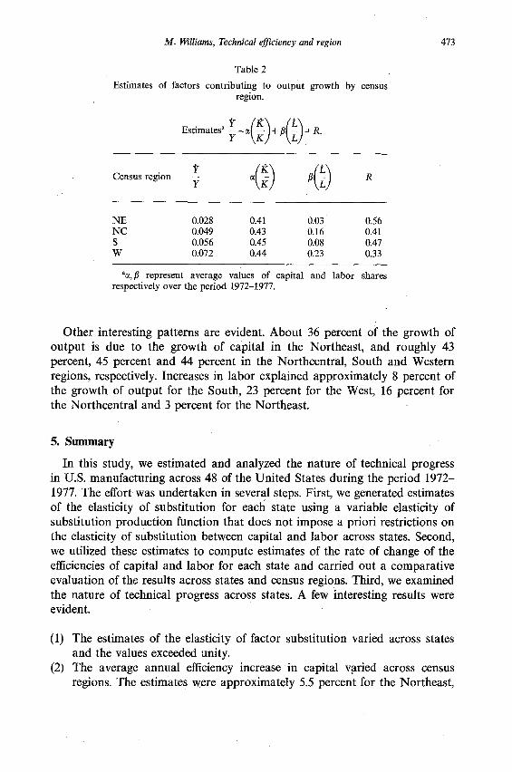
Table 1 reports estimates of the elasticity of substitution (s&, total factor productivity, (R,J, and the rates of change of the efficiency of capital (.@A) and labor (B/B) by region over the period 1972-1977. As found in many two- input (capital-labor) studies, capital and labor are substitutes.i’ Berndt and Wood (1975) reported estimates, using national data of 1.41.

Recall that the estimates of k/A and h/B are obtained by using eqs. (15) and (16). We examined and compared the results across the 48 states and found that the efticiency increase in capital is generally greater than the efficiency increase in labor. By census region, the average efficiency increase in capital was found to be approximately 5.5 percent in the Northeast, 5.3 percent in the Northcentral, 3.1 percent in the South and 5.6 percent in the West. The rates of change in the efficiencies of capital in the states of Mississippi, Texas, Oklahoma, Louisiana, Wyoming, Nevada, California, New York, New Hampshire, Vermont, Pennsylvania, Connecticut, Illinois, Wisconsin, and North Dakota are considerably higher than their regional averages. The estimated percent changes in the efficiency of labor are positive for some states and negative for others. The negative results may be due to difficulties in adjusting the level of employment to changes in economic conditions in these states. It may also be due to the nature of the data. Furthermore, the elasticity of substitution is positive, and the rate of change of wages is positive, thus the negative increase in the efficiency of labor in any state (B/B) may be due to changes in the ratio of output to labor. Negative technological augmentation for labor in a national study is also reported by Sato (1970).

The third and fourth columns R, and R, in table 1 show the percentage change in output not attributed to percent changes in inputs. The estimates of R, for each state are obtained directly from the data on output, capital, and labor. The measure R, is considered a measure of technical change

‘As noted in other studies that have used the translog functional form, the adding up constraint placed on the factor shares require that one equation be deleted.

“The parameter estimates used to compute sKL were obtained by using the 1977 cross-section data. The Zellner (1962) iterative estimation procedure was employed. This procedure assures that the estimates will be invariant to which share equation is deleted. Iteration and convergence yield the following maximum likelihood estimates:

ah Y ~ = 0.7558 +0.0828 In (L/K), alnL (11.04) (3.47)

Log of likelihood function = 75.268.

Estimates of sKL were also computed across states for 1972. The results were qualitatively similar. We choose to report those for 1977.

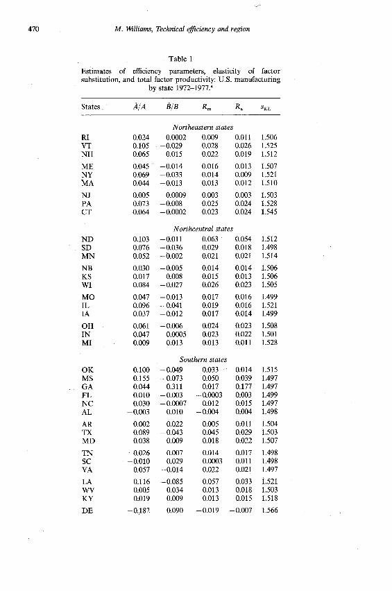
470 M. Williams, Technical eficiency and region

Table 1

Estimates of efficiency parameters, elasticity of factor substitution, and total factor productivity: U.S. manufacturing

by state 1972-1977.”

States

RI VT NH

ME

K

0.045 0.069 0.044

NJ 0.005 PA 0.073 CT 0.064

ND SD MN

NB KS WI

MO IL IA

0.047 0.096 0.037

OH 0.061 IN 0.047 MI 0.009

OK MS GA FL NC AL

AR TX MD

TN SC VA

LA WV KY

DE

0.024 0.105 0.065

0.103 0.076 0.052

0.030 0.017 0.084

0.100 0.155 0.044 0.010 0.030

-0.003

0.002 0.089 0.038

0.026 -0.010

0.057

0.116 0.005 0.019

-0.182

Northeastern states 0.0002 0.009 0.011

-0.029 0.028 0.026 -0.015 0.022 0.019

-0.014 0.016 0.013 -0.033 0.014 0.009 -0.013 0.013 0.012

0.0009 0.003 0.003 -0.008 0.025 0.024 -0.0002 0.023 0.024

zentral states -0.011 0.063 0.054 -0.036 0.029 0.018 -0.002 0.021 0.021

-0.005 0.014 0.014 0.008 0.015 0.013

-0.027 0.026 0.023

-0.013 0.017 0.016 -0.041 0.019 0.016 -0.012 0.017 0.014

-0.006 0.024 0.023 0.0005 0.023 0.022 0.013 0.013 0.011

1.506 1.525 1.512

1.507 1.521 1.510

1.503 1.528 1.545

1.512 1.498 1.514

1.506 1.506 1.505

1.499 1.521 1.499

1.508 1.501 1.528

Southern states -0.049 0.033 -0.073 0.050

0.311 0.017 -0.003 -0.0003 -0.0007 0.012

0.010 -0.004

0.022 0.005 -0.043 0.045

0.009 0.018

0.007 0.014

0.014 0.039 0.177 0.003 0.015 0.004

0.011 0.029 0.022

0.017 0.029 0.0003 0.011

-0.014 0.022 0.021

-0.085 0.057 0.033 0.034 0.013 0.018 0.009 0.013 0.015

0.090 -0.019 -0.007

1.515 1.497 1.497 1.499 1.497 1.498

1.504 1.503 1.507

1.498 1.498 1.497

1.521 1.503 1.518

1.566

M. Williams, Technical efficiency and region 471

Table 1 (continued)

States A/A B/B Rm Re SKL

NM WY NV

MT ID OR

UT CA co

AZ WA

-0.025 0.306 0.123

0.029 - 0.029

0.030

-0.003 0.079 0.034

0.002 0.073

Western states

-0.005 -0.134 -0.101 0.134 -0.039 0.055

0.016 0.025 0.042 0.002 0.012 0.020

-0.0001 -0.004 -0.033 0.024 -0.016 0.007

0.0001 0.0009 -0.007 0.034

-0.015 1.498 0.129 1.510 0.044 1.498

0.023 1.508 0.004 1.503 0.021 1.498

-0.002 1.497 0.018 1.503 0.006 1.512

0.001 1.497 0.030 1.501

NE NC S W

Regional average? 0.055 -0.012 0.017 0.016 1.517 0.053 -0.011 0.023 0.020 1.508 0.031 0.016 0.017 0.026 1.507 0.056 -0.012 0.024 0.024 1.502

‘Entries in columns 2 through 4 are average annual estimates over the time period. Estimates of sKL are derived from a cross-section of states using 1977 data.

“Note that NE, NC, S, and W denote Northeastern, Northcentral, Southern, and Western census regions respectively.

obtained as a residual. The other measure, R,, is obtained by using the estimates of k/A and l?/B.ll It can be seen that the measured R, is relatively close to the estimated R,. The estimated percentage rate of growth of total factor productivity is 1.7 percent per annum in the Northeastern region, 2.3 percent per year in the Northcentral and 2.4 in the Western regions, and around 1.7 percent in the Southern region. Since the estimates of R, are not dramatically different from those of R, across states and census regions, we may conclude that the estimates obtained for k/A and B/B are reasonable.

We now turn to the question of whether technical progress is labor-saving or capital-using over the time ,period across regions. We adopt the Hicksian definition of technical change, that is, technical change is labor-saving (capital-using) if at a constant capital-labor ratio, its effect is to increase the ratio of the marginal product of capital to labor so that capital is substituted for labor. Similarly, technical change is capital-saving (labor-using) if it

‘iconsider eq. (7). Y/Y= a(@K) + a(kl.4) + /?(t/L) + a(@B). This can be reformulated as follows: Y/Y-GI(&/K)-/J(.@!,) =a(k/A)+P(@B). The values on the left-hand side of this latter expression are provided in the original data. The values on the right-hand side are estimated.

412 M. Williams, Technical efficiency and region

lowers the ratio of the ,marginal product of capital to labor so that labor is substituted for capital. Let h denote the interest-wage rate ratio. Then h/h denotes the rate of change of that ratio over the period. From the foregoing analysis, consider eqs. (13) and (14). Subtracting (13) from (14) gives us an expression of h/h in terms of Z, k/A, B/B and i/x, that is

(31)

when x is constant, i/x is zero and h/h depends on estimates of k/A, BIB and sKL. Recall that sKL assumes different values. When sKL= 1, the second term on the right-hand side of (31) is zero and h/h=O; thus technical progress is neutral. When s,,> 1, the second term in the expression is greater than zero, and if the rate of change of the efficiency of capital (A/A) is greater than the rate of change of the efficiency of labor (B/B), then h/h>O, and technical change is labor-saving. Similarly, if the B/B >klA, technical change is capital saving. Finally, if sKL< 1, the second term in the expression is less than zero, and if B/B <k/A, then h/h<0 and technical change is capital-saving. But if BIB>k/A, then technical change is labor-saving.

The results in table 1 show that sKL is greater than unity for each state across census regions. Generally, k/A > BIB across states. Therefore, technical change across states within census regions over the period (1972-1977) tend to be capital-using.

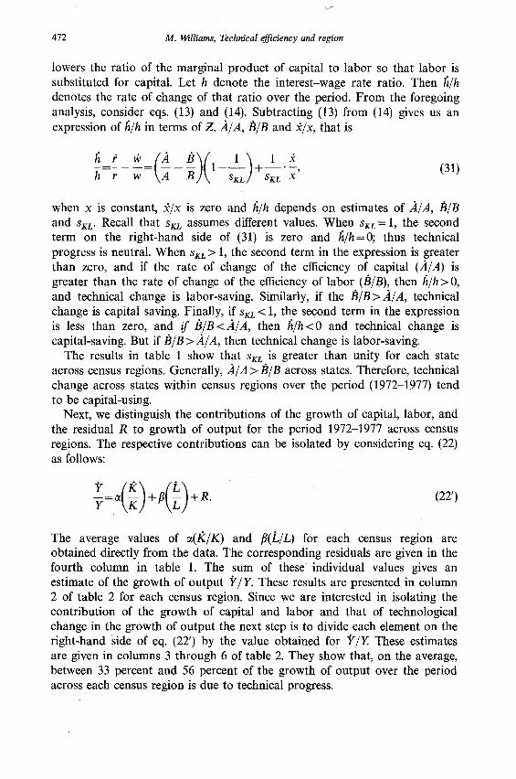
Next, we distinguish the contributions of the growth of capital, labor, and the residual R to growth of output for the period 1972-1977 across census regions. The respective contributions can be isolated by considering eq. (22) as follows:

$=.(;)+P(;)+R. GY

The average values of c&K) and /@&) for each census region are obtained directly from the data. The corresponding residuals are given in the fourth column in table 1. The sum of these individual values gives an estimate of the growth of output Y/Y. These results are presented in column 2 of table 2 for each census region. Since we are interested in isolating the contribution of the growth of capital and labor and that of technological change in the growth of output the next step is to divide each element on the right-hand side of eq. (22’) by the value obtained for Y/Y These estimates are given in columns 3 through 6 of table 2. They show that, on the average, between 33 percent and 56 percent of the growth of output over the period across each census region is due to technical progress.

M. WUliams, Technical efficiency and region 473

Table 2 Estimates of factors contributing to output growth by census

region.

Census region P 7 a(;) If;) R

NE 0.028 0.41 0.03 0.56 NC 0.049 0.43 0.16 0.41 S 0.056 0.45 0.08 0.47 W 0.072 0.44 0.23 0.33

‘G(,B represent average values of capital and labor shares respectively over the period 1972-1977.

Other interesting patterns are evident. About 36 percent of the growth of output is due to the growth of capital in the Northeast, and roughly 43 percent, 45 percent and 44 percent in the Northcentral, South and Western regions, respectively. Increases in labor explained approximately 8 percent of the growth of output for the South, 23 percent for the West, 16 percent for the Northcentral and 3 percent for the Northeast.

5. Summary

In this study, we estimated and analyzed the nature of technical progress in U.S. manufacturing across 48 of the United States during the period 1972- 1977. The effort was undertaken in several steps. First, we generated estimates of the elasticity of substitution for each state using a variable elasticity of substitution production function that does not impose a priori restrictions on the elasticity of substitution between capital and labor across states. Second, we utilized these estimates to compute estimates of the rate of change of the efficiencies of capital and labor for each state and carried out a comparative evaluation of the results across states and census regions. Third, we examined the nature of technical progress across states. A few interesting results were evident.

(1) The estimates of the elasticity of factor substitution varied across states and the values exceeded unity.

(2) The average annual efficiency increase in capital varied across census regions. The estimates were approximately 5.5 percent for the Northeast,

414 M. Williams, Technical efficiency and region

5.3 percent in the Northcentral, 3.1 percent in the South and 5.6 percent in the West. Generally, the efficiency increases in labor across regions tend to be smaller.

(3) The rates of change of total factor productivity were approximately 1.7 percent, on the average, in the Northeast, 2.3 percent in the North- central, 2.4 percent in the West, and 1.7 percent in the South.

(4) Increases in the labor explain approximately 8 percent of the growth of output in the South, 23 percent in the West, 16 percent in the Northcentral and 3 percent in the Northeast. Increases in capital explained between 41 and 45 percent of the growth of output across census regions. Finally, between 33 and 56 percent of the growth of output across census regions is due to technical progress.

This research does suggest that there is a way to separate out the efficiencies of capital and labor and the sources of output growth in an interregional context. The results can then be compared across states and census regions. Although we have used aggregated data we have observed some reasonable trends. However, the results may be sensitive to changes in the data. Additional research is needed using time series data for each state in order to provide more comparative evidence on interregional productive efficiencies.

Appendix: Derivation of elasticity of factor substitution

d In L/K WY, d(-VK) YL Wl~YdL SLK=dln(YJYK) =-LK’d(YL/YK)=-LK’d(YLIYK)/dL (A-1)

but

d(L/K)/dL = y --+KL+ W-0 lK K’

and

d(Y,/Y,)/dL= -d2YK/dY$(Y;Y,,-2Y,y,y,,+ Y;Y,,).

Combining these expressions gives

r, r,( Y,L + TICK) ‘““=L.K(Y;r,,-zr,r,Y,,+ YiY,,) (-4.2)

Since the production function is linearly homogeneous the numerator of

M. Williams, Technical eficiency and region 41.5

(A.2) becomes Y,Y,Y using Euler’s Theorem. For the denominator since Y(L,K) is homogeneous of degree 1, YL and Y, are homogeneous of degree zero. Applying Euler’s theorem to YL and Y, we have

and

y,,L + Y,,K E 0, (A.3)

Y,,K + Y,,L = 0. (A.4)

With the appropriate substitutions for YLL and Y,, using (A.3) and (A.4) the denominator becomes

LK( r; Y,, - 2 YL YK YLK = Y; Y,,) = Y,,( Y,L + Y,K)2 = - YLK Y2.

Therefore for a linear homogeneous production function

S - YLYXY YLYK

=K= - yLK y2 =Y.> (A.5)

which is a simplification of (A.l) and is equivalent to (12a).

References

Aberg, Reginald, Y., 1973, Productivity differences in Swedish manufacturing, Regional and Urban Economics 3, 131-156.

Batavia, Bala, 1979, The estimation of biased technical efficiency in the U.S. textile industry, 1949-1974, Southern Economic Journal 45, 1091-1100.

Berndt, Ernst R. and Laurits R. Christensen, 1973, The translog functions and the substitution of equipment, structures and labor in U.S. manufacturing: 1929-1968, Journal of Econometrics 1, 81-114.

Berndt, Ernst R. and David 0. Wood, 1975, Technology, prices and the derived demand for energy, Review of Economics and Statistics 57, 259-268.

Browne, Lynne, Peter Mieszkowski, and Richard F. Syron, 1980, Regional investment patterns, New England Economic Review, July-Aug., 5-23.

Denison, Edward F., 1962, The sources of economic growth in the United States and the alternatives before U.S., Supplementary paper no. 13 (Committee for Economic Development, Washington, DC).

Lianos, Theodore P., 1976, Factor augmentation in Greek maufacturing, 1958-1969, European Economic Review 8, 15-3 1.

Moomaw, Ronald L., 1981, Productive efficiency and region, Southern Economic Journal 48, 344-357.

Moomaw, Ronald L., 1983, Nonlabor income measures of capital intensity versus capital stock measures in estimating the determinants of regional labor productivity differentials: The manufacturing sector, Annals of Regional Science 17, 79-93.

Nadiri, Ishaq, 1970, Some approaches to the theory and measurement of total factor productivity: A survey, Journal of Economic Literature 4, 1137-l 177.

Nicholson, Norman, 1978, Differences in industrial production efficiency between urban and rural markets, Urban Studies 15, 91-95

Sato, Ryuzo, 1970, The estimation of biased technical progress and the production function, International Economic Review 11, 179-208.

Zellner, Arnold, 1962, An efficient model of estimating seemingly unrelated regressions and tests of aggregation bias, Journal of American Statistical Association 57, 977-992