technical efficiency of onion production in pakistan

University of Nebraska - Lincoln University of Nebraska - Lincoln

DigitalCommons@University of Nebraska - Lincoln DigitalCommons@University of Nebraska - Lincoln

Journal for the Advancement of Developing Economies Economics Department

2015

Technical Efficiency of Onion Production in Pakistan, Khyber Technical Efficiency of Onion Production in Pakistan, Khyber

Pakhtunkhwa Province, District Malakand Pakhtunkhwa Province, District Malakand

Abid Khan University of Agriculture, Peshawar–Pakistan

Follow this and additional works at: https://digitalcommons.unl.edu/jade

Part of the Econometrics Commons, Growth and Development Commons, International Economics

Commons, Political Economy Commons, Public Economics Commons, and the Regional Economics

Commons

Khan, Abid, "Technical Efficiency of Onion Production in Pakistan, Khyber Pakhtunkhwa Province, District Malakand" (2015). Journal for the Advancement of Developing Economies. 27. https://digitalcommons.unl.edu/jade/27

This Article is brought to you for free and open access by the Economics Department at DigitalCommons@University of Nebraska - Lincoln. It has been accepted for inclusion in Journal for the Advancement of Developing Economies by an authorized administrator of DigitalCommons@University of Nebraska - Lincoln.

https://digitalcommons.unl.edu/

https://digitalcommons.unl.edu/jade

https://digitalcommons.unl.edu/jade

https://digitalcommons.unl.edu/economicsdept

https://digitalcommons.unl.edu/jade?utm_source=digitalcommons.unl.edu%2Fjade%2F27&utm_medium=PDF&utm_campaign=PDFCoverPages

http://network.bepress.com/hgg/discipline/342?utm_source=digitalcommons.unl.edu%2Fjade%2F27&utm_medium=PDF&utm_campaign=PDFCoverPages








https://digitalcommons.unl.edu/jade/27?utm_source=digitalcommons.unl.edu%2Fjade%2F27&utm_medium=PDF&utm_campaign=PDFCoverPages

Journal for the Advancement of Developing Economies 2015 Volume 4 Issue 1 ISSN:2161-8216

4 Institute for the Advancement of Developing Economies 2015

Technical Efficiency of Onion Production in Pakistan, Khyber Pakhtunkhwa Province, District Malakand

Abid Khan

University of Agriculture, Peshawar–Pakistan ABSTRACT This research was conducted to estimate the technical efficiency and determinants of onion production, by using the Cobb-Douglas stochastic frontier production function with the inefficiency effects model. A multistage sampling technique was used to collect data, randomly, from 93 respondents. The empirical results showed that urea, farm yard manure (FYM), irrigation, and pesticides were the major factors that influence changes in onion production. Farm-specific variables such as education and area were found to have significant effects on the technical inefficiency among the onion producers. The technical efficiency of farmers varied from 0.7478 to 0.9851 with a mean technical efficiency of 0.9425. The implication of the study is that efficiency in onion production among the farmers could be increased by 6% through better use of urea, FYM, irrigation, and pesticides in the short term given the existing state of technology. The estimated gamma (γ) value was found to be 0.93, which shows that 93% variation in production of onions was due to inefficiency factors. In order to increase the production of onions by taking advantage of a high-efficiency level of the farmers, they should be motivated to adopt new techniques of farming and improved hybrid technology, by providing either formal or informal education Keywords: Cobb Douglas, gamma, Khyber Pakhtunkhwa, Malakand, multistage sampling, onion, stochastic frontier, technical efficiency. 1 INTRODUCTION Onions (Allium cepa L) are a vegetable largely produced and is used in all traditional cooking and gastronomic preparations in Pakistan and also across the whole world. It is also an important kitchen item for daily use (Hussain, 2001). It is consumed with a variety of dishes as a vegetable and also used for salads. It helps to act as a guard for many chronic diseases. It also helps in lowering blood pressure and cholesterol levels because they contain naturally-occurring chemicals known as organosulfur compounds. Hussain (2001) also reported that there are no fats and cholesterol in onions and they contain those vitamins and chemicals which help the free radicals of the human body to be figured. According to the Food and Agriculture Organization of the United Nations (FAO) estimation, about 140 countries grow storage-dry onions and 55 countries grow green onions (including shallots). In 2010, the global production of storage-dry onions totaled 74.3 million tons and green onions (including shallots) totaled 3.6 million tons. China was a leading producing country in 2010 with a total production of 20.5 million tons of storage-dry onions, followed by India, USA, Egypt, Iran,

proyster2

Typewritten Text

doi:10.13014/K2PZ5715

Journal for the Advancement of Developing Economies 2015 Volume 4 Issue 1

Page 25 Institute for the Advancement of Developing Economies 2015

Turkey, Pakistan, Brazil, the Russian Federation, and the Republic of Korea (Food and Agriculture Organization of the United Nations, 2010). The production of onions in Asian countries is more than 50% (14.6 million tons) of the total world production, including shallots. So that’s why the Asian countries have a contribution of about one fourth (2.3 million tons) to the total global trading of onions. Pakistan not only stands with the top onion-producing countries of the world but also placed among the countries having higher consumption levels per capita. On the average, about 47.7 billion kg’s of onion is consumed each year around the world, leading to an approximate value of 6.5 kg’s per capita each year. In Pakistan the consumption of onion per capita was reported to be about 11 kg’s s per year. But the highest level of onion consumption per capita was reported for Turkey and Libya with an approximate value of 36.6 kg and 32 kg, respectively, per year (Food and Agriculture Organization of the United Nations, 2010). Sindh province contributed 39% to the total onion production of Pakistan while the contribution of Balochistan, Punjab, and Khyber Pakhtunkhwa is 35%, 18%, and 8% respectively. As far as the increase in area and production of onions is concerned, Saqib (2012) reported over 127.8 thousand hectares and 1.7 million tons, respectively, with 13.8 tons per hectare yield. For most Pakistani farmers, onions are valuable commodities for trading, so for the fulfillment of domestic demand onions needs to be imported. But the availability is not even the fourth part of an onion per head for a day (Hussain, 2001). The availability of onions will not only increase but the income level of the farmers will also be raised, if productivity of onion is enhanced, by applying modern practices of farming. As onion production needs more laborers, unemployment levels will decrease (Abedullah & Farooq 2002, Barron & Rello, 2000). Analysis of the efficiency of agricultural production is a key problem in third world countries. In order to achieve higher domestic production of onion crops, productivity of onion needs to be increased; productivity can be promoted by adopting new techniques or by improving efficiency or both. Most of the farmers in Pakistan are reluctant to adopt modern technology. Therefore, to increase the productivity of agricultural crops in the short run, the level of efficiency must be improved (Javed, Adil, Javed, & Hassan. 2008). Increase in productivity and growth in production of the agricultural sector leads to an effective strategy for economic development (Bravo-Ureta & Pinheiro, 1997). Efficiency analyses trace back to Knight (1933), Debreu (1951), and Koopmans (1951). A definition of technical efficiency was provided by Koopmans (1951) while its first measure of the “coefficient or resource utilization” was introduced by Debreu (1951). Farrell (1957) in a seminal paper, following Debreu (1951), provided a definition of frontier production functions, which embodied the idea of maximization (Shuwu, 2006). Farrell (1957) also introduced efficiency for the first time and found that economic efficiency is the measure of technical and allocative efficiency. The ability of a firm to produce the maximum possible output from the given set of inputs and technology is called technical efficiency, while the ability of a firm to remain on the same production possibility curve by using the least cost combination of inputs and available technology is called allocative efficiency.



The objective of this research study is to identify those factors which affect the technical efficiency of onion growers and providing them the opportunity to increase their output. The results of this research will also provide help for policy makers to initiate programs related to the effective expansion of onion production. Therefore, the aim of this research is to analyze the technical efficiency of different resources used in the production mechanism of onions in Khyber Pakhtunkhwa. 2 DATA COLLECTION AND SAMPLE SIZE This study was carried out in the District Malakand of Khyber Pakhtunkhwa province, Pakistan. The multistage sampling technique was used for the selection of sample size. In the first stage, district Malakand was purposively selected because it is one of the major onion-producing districts of Khyber Pakhtunkhwa (GoP, 2012). In the second stage, one Tehsil was randomly selected. Then in the third stage, one union council was randomly selected. In stage four, three villages, namely Zormandi, Palonow and Naray Oba, which have the same geographical, economical, and social impact on onion production, were randomly selected. Ninety-three onion growers were selected through the proportional allocation sampling technique as follows (Cochran, 1977): n" = n/NxN( (1) Where, ni = number of onion growers in the ith village, n = total sample size, N" = total number of onion growers in the ith village, and N = total number of onion growers. Primary data for this study were collected through well-structured questionnaires during 2012 and 2013, while secondary data were collected from official sources, e.g. the government of Pakistan’s economic survey (2012) and the Food and Agriculture Organization (2010). An interview schedule was prepared in the light of study objectives. The primary data regarding onion yield, inputs used in the production process (i.e. seed rate, tractor hours, labor man days, urea, farm yard manure, and pesticides), and other factors involved in the production process i.e. age, education, farming experience, and area under onion, were collected from 93 onion growers. In order to measure the relationship between output of onion and input used in onion production, and the mean technical efficiency and technical inefficiency of onion production, the ML estimates of the stochastic frontier model were used for the analysis of data. 3 MODEL SPECIFICATION The functions for the average production have been estimated by econometricians for a long time. To link theory with empirical work, considerations have been given to the possibility of estimating the frontier production function after the pioneer work of Farrell (1957) (Aigner, Lovell, & Schmidt 1977). Aigner et al. (1977) and Meeusen & Van den Broeck (1977) independently suggested the stochastic frontier production function. The function for the stochastic production is given below:



Y" = f(X";β") + e" i = 1, 2, 3,………., n (2) Where, Y" represents output level of onions for the ith farm in Kgs/ha, f(X; ß) is a suitable CobbDouglas production function of vector, X", of inputs used in production of onion in units/ha for the ith farm, β" are the unknown parameters which is to be estimated, e" is an error term composed of two components: v" is a random error either associated with measurement error in the production of onions reported or the effects of those variables which are excluded from the production function. The u" is assumed to be a non-negative truncated half normal, N(0,σ²u) is a random variable associated with farm-specific factors, which shows that ith farm is hardly attaining the maximum efficiency of onion production, so, the u" is associated with the technical inefficiency and has a value between zero and one. Therefore, the specified empirical model of the Cobb-Douglas production function for onion production is given as follows: ln Yld = β6 +β7 ln 𝑆𝑑𝑟 +β;lnTtrctrHrs +βBlnTLbr +βElnUr +βGlnFYM +βJlnIrri + βMlnPest + e" (3)

Where, ln = natural logarithm, Yld = yield of onion in kg per hectare, Sdr = seed rate used in kg per hectare, TtrctrHrs = total tractor hours used per hectare, TLbr = total labor man days per hectare, Ur= urea used in kg per hectare, FYM = farm yard manure used in kg per hectare, Irri = number of irrigations per season, Pest = volume of pesticides and weedicides used for one hectare, β" = unknown parameters to be estimated, and e" = composed error term. According to Battese and Coelli (1995) the inefficiency model was specified as follows: µ" = g(Z" ∶ δ") (4) µ" = δ6 +δ7AGE +δ;EXPE +δBEDUC +δEAREA +ω" (5) Where, µ"= the error term of technical inefficiency, δ" = coefficients to be estimated, AGE = age of the onion growers in years, EXP = farming experience of the onion growers in years, EDU = education of the onion growers in years, AREA = area under onion crop in hectare, and ω" = random error term. Technical efficiency for the ith farmer may be defined as, the ratio of observed production to the corresponding frontier production, and can be expressed as follows: TE" = Y[\/Y]\ = [f(β, X) +(Vi + Ui)]/[f(β, X) + (Vi)] (6) Where, Y[\ is the observed production of the individual farmer, and Y]\ is the frontier production, the maximum production that a farmer can obtain from the given resources. The value of TE lies between 0 and 1. 4 LOG LIKELIHOOD RATIO TESTS FOR HYPOTHESES TESTING The formula for the LR test statistic is as under:



LR statistic (λ)= 2[lnH6/lnH7] = -2[lnH6-lnH7] (7)

Where, lnH0 is the null hypothesis which denotes the value of the log likelihood function, when it is assumed that inefficiency is not present and, lnH1 is the alternative hypothesis which denotes the value of the log likelihood function, when it is assumed that inefficiency is present in the model. LR statistic (λ) follows a chi-square distribution with degrees of freedom equal to the number of restrictions imposed on the model. If the value of the LR statistic (λ) is significant, then we will reject the null hypothesis that inefficiency is not present in favor of the presence of inefficiency. 5 MODEL ADEQUACY TESTS HETEROSCEDASTICITY The assumption of the homoscedasticity of the classical linear regression model is that the variance of each disturbance term µi for the chosen values of the dependent variables is a constant number equal to σ². Symbolically it can be written as: E(µ"²) = σ² i = 1,2,…..,n (8) If the above-mentioned assumption is violated then it will lead to a problem of heteroscedasticity, which means that variance of the error term will no longer remain constant. The consequence of heteroscedasticity is an unbiased but inefficient estimate of the coefficients. The results of the variances which may be small or large, lead to type I or type II error in the presence of heteroscedasticity, meaning that OLS is not BLUE (Best Linear Unbiased Estimator). Heteroscedasticity is mainly present in cross sectional data, as ours, then it is in time series data (Gujarati & Porter, 2009). To detect the heteroscedasticity, in our data, the Goldfeld Quandt test and Breusch-PaganGodfrey tests were used. Goldfeld Quandt Test for Heteroscedasticity The procedure of the Goldfeld Quandt test is as follows:

1. Data was arranged in ascending order according to explanatory variables. 2. The data was divided into two groups each of (n – c)/2 observations, after omitting the central

values c (c = 17) 3. Regression was run for each of the (n – c)/2 observations and the residual sum of squares

(RSS) for each regression was obtained i.e. RSSde for smaller values and RSSfe for larger values. Each RSS has (n – c – 2k)/2 df, where k is the number of parameters including the intercept.

4. Considering the assumption of normal distribution of “µ"” and homoscedasticity, the value of

“λ” was calculated as: λ = RSSfe/df ÷ RSSde/df, which follow the F-distribution with (n – c – 2k)/2 df for numerator and denominator respectively. If the value of F- calculated (λ) is greater than the value of F-tabulated at the suggested level of significance, then we will reject the hypothesis of homoscedasticity otherwise not (Gujarati & Porter, 2009).



i

Breusch-Pagan-Godfrey Test for Heteroscedasticity To explain this test, the following method was adopted, by considering the regression model (3) as given above: 1. The regression for model (3) was run by OLS and the error terms µ7, µ; ……………. µg were

obtained. 2. σ² was calculated as: σ² = Σµ"²/n (9) 3. “v"” variable was constructed as: v" =µ"²/ σ² 4. 5. Then the regression “v"” was run on B’s as fallows.

(10)

v" = α6 +α7B7 +α;B; +αBBB +αEBE +αGBG +αJBJ +αMBM + p" (11) Where pi is the error term for the above regression. 6. The explained sum of square (ESS) was obtained from the regression of eq. (11) and θ was

calculated as: θ = 1/2(ESS). If the normal distribution of µi is considered, there is no heteroscedasticity, and the sample size n increases, then θ~X²m-1, which shows that θ follows the chi-square distribution with m-1 df. Now, if the calculated chi-square value (=θ) exceeds the critical chi-square value (=X²) at the chosen level of significance, then one must reject the hypothesis of homoscedasticity. (Gujarati & Porter, 2009).

Multicollinearity One of the assumptions of the classical linear regression model (CLRM) is that the explanatory variables (X,s) should not be collinear. If this assumption is violated, then we are facing a problem of multicollinearity. In order to detect such problem, tests like correlation matrix and auxiliary regression were used (Gujarati & Porter, 2009). Correlation matrix Correlation means the positive (direct) or negative (inverse) interrelationships between the explanatory variables in a model. To draw the correlation matrix for our data, k(k-1)/2 (k = number of variables), zero order correlation coefficients were estimated and then put into a matrix called correlation matrix “M” as follows: M = From the above matrix we can estimate the correlation coefficients of the explanatory variables. r7; indicates the correlation coefficient between X7 and X; and so on (Gujarati & Porter, 2009). Auxiliary regression Multicollinearity is a result from the exact or approximate linear combination of one or more explanatory variables. To find this combination, each explanatory variable (X") was regressed on the remaining explanatory variables, and the corresponding R; was found, written as R(;; each of these regressions were termed as auxiliary regression.



Now, the relationship between F and R2 can be established as: Fi = R2x1,x2….x7/(k-2) ÷ (1- R2x1,x2….x7)/(n-k+1) (12) It follows the F distribution with k-2 and n-k+1 df. In the above model “n” is the sample size and “k” is the number of regressors including the intercept and Rk7k;…kM; is the coefficient of determination for each auxiliary regression. From the above model, if the calculated Fi value exceeds the critical F value at the chosen level of significance, then a particular regressor will be collinear with other regressors and, if not, then we will retain that particular variable (Gujarati & Porter, 2009). 6 RESULTS AND DISCUSSION Result of Goldfeld Quandt test for heteroscedasticity Following the method of the test, the result of λ (F-calculated), at 5% level of significance, is 2.048 with 30df. The critical F value at 5% level of significance with 30 df in the numerator and denominator is 2.390, so our calculated result is insignificant, therefore we accept the hypothesis of homoscedasticity for our data. Result of Breusch-Pagan-Godfrey (BPG) test for heteroscedasticity Following the method of the test, the calculated chi-square value (=θ) is 12.302. Now the 5% critical chi-square value (=X²) with 7 df is 14.0671. So, we accept the hypothesis of homoscedasticity (Table 1). Table 1: Result of Breusch-Pagan-Godfrey (BPG) test for heteroscedasticity

Variables Parameters Co-eff. Std. error t-ratios Constant β0 6.258 0.331 18.904 lnSdr β1 -0.066 0.085 -0.775 lnTtrctrHrs β2 0.070 0.059 1.187 lnTLbr β3 0.022 0.028 0.770 lnUr β4 0.016 0.011 1.385 FYM β5 0.099 0.043 2.290 lnIrri β6 0.772 0.112 6.898 lnPest β7 0.120 0.104 1.151 N 93 Df 7 RSS (Σ µi²) .613 σ2(Σ µi²/n) .007 Estimation of Theta (θ) Constant β0 2.256 6.907 0.327 lnSdr β1 3.801 1.780 2.135 lnTtrctrHrs β2 -0.902 1.242 -0.726 lnTLbr β3 -0.442 0.591 -0.749



lnUr β4 0.269 0.237 1.132 FYM β5 0.165 0.900 0.184 lnIrri β6 -2.357 2.333 -1.010 lnPest β7 -0.323 2.174 -0.149 ESS 24.604 Df 7 θ (ESS/2) 12.302

Source: Estimated from Survey Data, 2012-13 Result of correlation matrix The result of correlation matrix revealed that, out of seven variables, four variables had values greater than 0.80 and showed a correlation with other variables as given in Table 2. Table 2: Result of correlation matrix lnSdr lnTtrctrHrs lnTLbr lnUr lnFYM lnIrri lnPest lnSdr 1.0000 - - - - - - lnTtrctrHrs 0.8339 1.0000 - - - - - lnTLbr 0.3003 0.2507 1.0000 - - - - lnUr 0.1188 0.0921 0.0743 1.0000 - - - lnFYM 0.5426 0.4075 0.3860 0.1321 1.0000 - - lnIrri 0.8285 0.6793 0.3548 0.1265 0.5908 1.0000 - lnPest 0.8328 0.6666 0.3096 0.1490 0.5982 0.9479 1.0000

Source: Estimated from Survey Data, 2012-13. Result of auxiliary regression The results in Table 3 shows that the computed F" values are greater than the F-tabulated at 5% level of significance with 6 and 86 df in the numerator and denominator, respectively, with the exception of only one F value that is FE. So, it indicates the presence of a multicollinearity problem. But here we also note that the R"; values obtained from the auxiliary regression is not greater than the overall R; (0.906). So here multicollinearity is not a troublesome problem (Gujarati &Porter, 2009). Table 3: Result of auxiliary regression

R21 R22 R23 R24 R25 R26 R27 0.8379 0.7030 0.1899 0.0288 0.4118 0.9101 0.9075

Fi = R2x1,x2….x7/(k-2) ÷ (1- R2x1,x2….x7)/(n-k+1) F1 F2 F3 F4 F5 F6 F7

74.0971 33.9205 3.3608 0.4251 10.0347 145.1403 140.7003 Source: Estimated from Survey Data, 2012-13. Remedial measures for multicollinearity There are various measures to overcome this problem, i.e. dropping a variable, or collecting new data, etc. We did nothing with our data because, according to Blanchard, “multicollinearity is basically a problem of data deficiency and sometimes the researchers have no choice over the data that is available for the empirical analysis” (Gujarati & Porter, 2009).



Result of log likelihood ratio test for hypotheses testing From equation (7) the estimated value for LR statistic (λ) is 13.25, which is significant at 5% level of significance with six numbers of restrictions. So, we reject the null hypothesis of no inefficiency in the model in favor of the presence of inefficiency. Factors of Technical Efficiency The factors of technical efficiency were taken as seed rate, tractor hours, labors, urea, FYM, irrigation, and pesticides as shown in the first part of Table 4. The coefficient for the seed rate is positive which shows a positive effect on the production of onions but statistically it is insignificant. The same result was also estimated by Rahman & Umar (2005). For land preparation, tractor hours have positive but statistically insignificant coefficient, which shows a positive relationship between ploughing by tractor and yield. The coefficient of labors is positive and statistically insignificant, which shows a positive impact on the production of onions. This result is the same as the results of Adewumi & Adebayo (2008), and Dlamini, Rugambisa, Masuku, and Belete (2010). The coefficient of urea is positive and statistically significant. The same results were also found by Obwona (2006), Wakili (2006), Dlamini et al. (2010), and Okon, Enete, and Bassey (2010). The coefficient of FYM is positive and statistically significant, and the same as that of the result of Shaheen, Anwar, and Hussain (2006) and Okon et al. (2010). Irrigation is statistically significant with a positive coefficient. It shows that a 1% increase in irrigation will increase the production of onions by 0.70%. This result is the same as the results of Shaheen et al. (2006), and Bakhsh (2007). The coefficient of pesticides is positive and statistically significant and implies that one percent change in pesticides will increase the production of onions by 0.12%. lt is the same as the result of Wakili (2010). Factors of Technical Inefficiency The factors of technical inefficiency were age, farming experience, education and area as shown in the second part of Table 4. The coefficient of age for growers is positive and insignificant, which shows a positive but insignificant relationship with technical inefficiency. This result is the same as found by Fasasi (2007), and Sadiq et al. (2009). The coefficient of farming experience is negative and statistically insignificant and shows a negative but insignificant relationship with technical inefficiency. The same result was also found by Msuya and Ashimogo (2005), Fasasi (2007), and Rahman and Umar (2009).



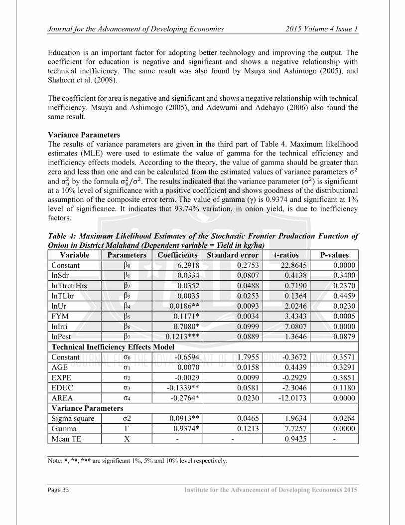
Education is an important factor for adopting better technology and improving the output. The coefficient for education is negative and significant and shows a negative relationship with technical inefficiency. The same result was also found by Msuya and Ashimogo (2005), and Shaheen et al. (2008). The coefficient for area is negative and significant and shows a negative relationship with technical inefficiency. Msuya and Ashimogo (2005), and Adewumi and Adebayo (2006) also found the same result. Variance Parameters The results of variance parameters are given in the third part of Table 4. Maximum likelihood estimates (MLE) were used to estimate the value of gamma for the technical efficiency and inefficiency effects models. According to the theory, the value of gamma should be greater than zero and less than one and can be calculated from the estimated values of variance parameters σ; and σn; by the formula σo;/σ;. The results indicated that the variance parameter (σ;) is significant at a 10% level of significance with a positive coefficient and shows goodness of the distributional assumption of the composite error term. The value of gamma (γ) is 0.9374 and significant at 1% level of significance. It indicates that 93.74% variation, in onion yield, is due to inefficiency factors. Table 4: Maximum Likelihood Estimates of the Stochastic Frontier Production Function of Onion in District Malakand (Dependent variable = Yield in kg/ha)

Variable Parameters Coefficients Standard error t-ratios P-values Constant β0 6.2918 0.2753 22.8645 0.0000 lnSdr β1 0.0334 0.0807 0.4138 0.3400 lnTtrctrHrs β2 0.0352 0.0488 0.7190 0.2370 lnTLbr β3 0.0035 0.0253 0.1364 0.4459 lnUr β4 0.0186** 0.0093 2.0246 0.0230 FYM β5 0.1171* 0.0034 3.4343 0.0005 lnIrri β6 0.7080* 0.0999 7.0807 0.0000 lnPest β7 0.1213*** 0.0889 1.3646 0.0879 Technical Inefficiency Effects Model Constant σ0 -0.6594 1.7955 -0.3672 0.3571 AGE σ1 0.0070 0.0158 0.4439 0.3291 EXPE σ2 -0.0029 0.0099 -0.2929 0.3851 EDUC σ3 -0.1339** 0.0581 -2.3046 0.1180 AREA σ4 -0.2764* 0.0230 -12.0173 0.0000 Variance Parameters Sigma square σ2 0.0913** 0.0465 1.9634 0.0264 Gamma Γ 0.9374* 0.1213 7.7257 0.0000 Mean TE X - - 0.9425 -

Note: *, **, *** are significant 1%, 5% and 10% level respectively.



Table 4 shows the ML estimations of the stochastic frontier Cobb-Douglas production function. It was found that FYM, irrigation, and pesticides were statistically significant at the 1%, 5%, and 10% level of significance with positive coefficients. The inefficiency model shows that education and area are statistically significant at 1% and 5% level of significance respectively, with negative coefficients. The ML estimations of Frontier 4.1 estimate a positive coefficient of variance parameter (σ;), which is significant at 5% level of significance. The value of gamma (γ) is 0.9374 and significant at 1% level of significance. It shows that 93.74% variation in the yield of onion is due to inefficiency factors. Frequency Distribution of Technical Efficiency of Onion Growers Table 5 shows the frequency distribution of technical efficiencies of onion growers. The minimum and maximum values of technical efficiencies are 0.7478 and 0.985, respectively, with a mean efficiency of 0.9425. So, these results indicate that by using the available inputs the yield of onion can be enhanced. Table 5: Frequency distribution of technical efficiency of onion growers

Technical efficiency Frequency Percentage <0.80 2 2.15 0.81 - 0.90 13 13.98 >0.90 78 83.87 Minimum 0.7478 - Maximum 0.9851 - Mean 0.9425 -

Source: Estimated from Survey Data, 2012-13. 7 CONCLUSION AND RECOMMENDATIONS The purpose of this study was to estimate technical efficiency of onions and the factors influencing the technical efficiency of onions in the Malakand district in Khyber PakhtunkhwaPakistan. The Cobb Douglas production function for stochastic frontier was used for the estimation of the technical efficiency of onions. The overall mean technical efficiency of 94.25% achieved by onion growers showed that there was some scope to increase onion production. The more important contributors in onion production were urea, farm yard manure (FYM), irrigation, and pesticides. Thus, an appropriate amount of utilization of these input variables could increase onion production. The results of the stochastic frontier production function and technical inefficiency model indicated that the estimated production elasticity for the irrigation variable of onion growers was higher (0.7080). The variable for urea, FYM, irrigation, and pesticides were positive and statistically significant according to an asymptotic t-test. Production elasticity for urea (0.0186), FYM (0.1171), irrigation (0.7080), and pesticides (0.1213) were important in terms of contribution towards higher onion yield. An attempt was made to determine the factors affecting technical efficiency in onion production. Farm- and farmer-related socioeconomic factors were included in the technical inefficiency model. The effect of education and area under onions had a negative and significant influence on technical inefficiency of onion farmers. So, it is concluded that the technical inefficiency of onions decreases



significantly with increase in area, implying that farmers with more area under onions are more efficient. The efficiency of onions is limited to the range of 0.20 hectare to 2.43-hectare land utilization. The educational level of farmers had contributed significantly to technical efficiency. It is estimated that inefficiency in onion production could be reduced by educating the onion farmers in improved techniques and proper use of available resources to boost their experience in onion production, hence policies designed to educate onion farmers through proper agricultural extension services could have a great impact in increasing the level of technical efficiency and hence the increase in onion productivity. As the famers were growing local varieties, the government should provide improved seed varieties of onions to the famers, either by payment in installments or at low prices, to increase the productivity of onions. In the study area, all the farmers were using tube well as a source of irrigation. Due to high prices of oil and shortage of electricity in the country, they were facing problems to irrigate the farms on specified times. So, the government should provide alternatives, e.g. canal irrigation or installation of solar system to generate power and solve the irrigation problem of the famers. The government should provide more funds to the extension workers to educate the farmers, by field demonstrations and farm visits, about new technologies and farming techniques. REFERENCES Abedullah, S. S., & Farooq, U. (2002). The vegetable sector in Indonesia: Farm and household

perspective on poverty alleviation. Asian Vegetable Research and Development Center (AVRDC), Taiwan-Asian Regional Center (ARC), Thailand. Technical Bulletin, 27, 31- 73.

Adewumi, M. O., & Adebayo, F. A. (2008). Profitability and Technical Efficiency of Sweet Potato Production in Nigeria. Journal of Rural Development, 31(5), 105-120.

Aigner, D. K., Lovell, C. K., & Schmidt, P. (1977). Formulation and Estimation of Stochastic: Frontier Production Function Models. Journal of Econometrics, 6, 21-37.

Bakhsh, K. (2007). An analysis of technical efficiency and profitability of growing potato, radish, carrot and bitter gourd: A case study of Pakistani Punjab (Unpublished PhD thesis). University of Agriculture, Faisalabad.

Barron, M. A., & Rello, F. (2000). The impact of the tomato agro-industry on the rural poor in Mexico. Agricultural Economics, 23, 289-297.

Battese, G. E., & Coelli, T. J. (1995). A Model for Technical Inefficiency Effects in a Stochastic Frontier Production Function for Panel Data. Empirical Economics, 20, 325-332.

Bravo-Ureta, B. E., & Pinheiro, A. E. (1997). Technical, Economic and Allocative Efficiency in Peasent Farming: Evidence from the Domain Republic. The Developing Economies, 35, 48-67.

Cochran, W. G. (1977). Sampling Techniques (3rd ed.). New York: John Wiley and Sons, New York.

Debreu, E. (1951). The Coefficient of Resource Utilization. Econometrica, 19, 273–292. Dlamini, S., Rugambisa, J. I., Masuku M. B., & Belete, A. (2010). Technical Efficiency of the Small-Scale Sugarcane Farmers in Swaziland: A Case Study of Vuvulane and Big Bend

Farmers. African Journal of Agricultural Research, 24(3), 329-338. Farrell, M. J. (1957). The Measurement of Productive Efficiency. Journal of the Royal Statistical

Society, 120(3), 253-281.



Fasasi, A. R. (2007). Technical Efficiency in Food Crop Production in Oyo State, Nigeria. Journal of Human Ecology, 22(3), 245-249.

Food and Agriculture Organization of the United Nations. (2010). http://www.fao.org/home/en/. Government of Pakistan. (2012). Agricultural Statistics of Pakistan. Retrieved from

http://www.gilanifoundation.com/homepage/Free_Pub/AGRI/AGRICULTURAL_STATI STIC S_OF_PAKISTAN_2010_2011.pdf

Gujarati, D. N., & Porter, D. C. (2009). Basics Econometrics (5th ed.). New York: McGraw Hill. Husain, S. S. (2001). Not Even a Quarter of an Onion a Day. Pakistan Journal of Agriculture Economics, 4(1), 15-24.

Javed, M. I., Adil, S. A., Javed, M. S., and Hassan, S. (2008). Efficiency Analysis of Rice-Wheat system in Punjab Pakistan. Pakistan Journal of Agricultural Sciences, 45 (3), 95-100.

Knight, F. 1933. The Economic Organization. New York: Harper and Row. Koopsman, T. C. (1951). An Analysis of Production as an Efficient Combination of Activities.

In T. C. Koopsman (Ed.), K. C. Activity Analysis of Production and Allocation. New York: Cowles NY Meeusen, W., & Van den Broeck, J. (1977). Efficiency Estimation from Cobb-Douglas

Production Functions with Composed Error. International Economics Review, 18, 435- 444. Msuya, E., & Ashimogo, G. (2005). Estimation of Technical Efficiency in Tanzanian Sugarcane

Production: A Case Study of Mtibwa Sugar Estate Outgrowers Scheme. Munich Personal Repec Archive, Paper No. 3747.

Obwona, M. (2006). Determinants of Technical Efficiency Differentials amongst Small and Medium- Scale Farmers in Uganda: A Case of Tobacco Growers. African Economic Research Consortium, Nairobi, Paper 152.

Okon, U. E., Enete, A. A., & Bassey, N. E. (2010). Technical Efficiency and its Determinants in Garden Egg (SolanumSpp) Production in Uyo Metropolis, AkwaIbom State, Nigeria. Field Actions Science Reports, Special Issue, 1, 1-6.

Rahman, S. A., & Umar, S. H. (2005). Measurement of Technical Efficiency and its Determinants in Crop Production in Lafia Local Government Area of Nasarawa State, Nigeria. Agro-Science, 8(2), 90-96.

Sadiq, G., Haq, Z., Ali, F., Mahmood, K., Shah, M., & Inamullah, K. (2009). Technical Efficiency of Maize Farmers in Various Ecological Zones of AJK. Sarhad Journal of Agriculture, 25(4), 607610.

Saqib, M. O. (2012, October 7). Onion Crop Escapes Monsoon Damage. Dawn. Shaheen, S., Anwar, S., & Hussain, Z. (2011). Technical Efficiency of Off-Season Cauliflower

Production in Punjab. Journal of Agricultural Research, 49(3), 391-406. Shuwu, H. T. (2006). Profit Efficiency among Rice Producers in Eastern and Northern Uganda.

(Unpublished PhD thesis). Makerere University, Uganda. Wakili, A. M. (2012). Technical Efficiency of Sorghum Production in Hong Local Government

Area of Adamawa State, Nigeria. Russian Journal of Agricultural and Socio-Economic Sciences, 6(6), 10-15.

technical efficiency of onion production in pakistan

Documents