technical memorandum 33-753 - nasa · technical memorandum 33-753 ... (jet propulsion lab.) 87 p hc...

N7621678illlHIIINIIIHHIIH

NATIONAL AERONAUTICS AND SPACE ADMINISTRATION

Technical Memorandum 33-753

On the Thermoelastic Analysis of Solar Cell Arrays

and Related Material Properties

M. A. Salama

F. L. Bouquet

(_ASA-CF-146579) ON _HE THERSOELASTI£

.%N_LYSIS OF SOLAE CELI ARF:AYS AND PELATED

ZAT_F[_[ FFOPEFTIES (Jet Propulsion Lab.)87 p HC $5.00 CSCL IOA

JET PROPULSION LABORATORY

CALIFORNIA INSTITUTE OF TECHNOLOGY

PASADENA, CALIFORNIA

February 15, 1976

G314q

N76-21678

Unclas

21507

https://ntrs.nasa.gov/search.jsp?R=19760014590 2018-08-27T11:27:49+00:00Z

- Page i of 2

TECHNICAL REPORT STANDARD TITLE PAGE

i. Report No. 33-753 2. Government Accession No.

4. Title and Subtitle

ON THE THERMDELASTIC ANALYSIS OF SOLAR CELL

ARRAYS AND R_ATED MATERIAL PROPERTIES

3. Recipient's Catalog No.

5. Report DateFebruary 15, 197(

6. Performing Organization Code

7. Author(s) 8. Performing Organization Report NoM. A. Salama, F. L. Bouquet

IO. Work Unit No.9. Per_rming Organization Name and Address


California Institute of Technology

4800 Oak Grove Drive

Pasadena, California 91103

12, Sponsoring Agency Name and Addre_


Washington. D.C. 20546

11. Contract or Grant No.

NAS 7-100

13. Type of Report and Period Covered

Technical Memorandum

14. Sponsoring Agency Code

15. Supplementary Notes

16. Abstract

Accurate prediction of failures of solar cell arrays requires corresponding

accuracy in the computation of their thermally induced stresses. This was

accomplished by usingthe finite element technique. Certain improvements

in the previously reported procedures for stress calculation were intro-

duced together with failure criteria capable of describing a wide range of

ductile and brittle material behavior. With these improvements and capa-

bilities, the stress distribution and associated failure mechanisms in the

N-interconnect Junction of two JPL solar cell designs were discussed and

correlated to previous findings.

In such stress and failure analysis, it is essential to know the thermo-

mechanical properties of the materials involved. To complement previous

efforts in this direction, new measurements were made of properties of

materials suitable for the design of lightweight arrays: namely, the

microsheet-0211 glass material for the solar cell filter together with

five materials for lightweight substrates (Kapton-H, Kapton F, Teflon,

Tedlar, and Mica Ply PG-402). The temperature-dependence of the thermal

coefficient of expansion for these materials was determined together with

other key properties such as the elastic moduli, Poisson's ratio, and thestress-strain behavior up to failure.

17. Key Wor_ _elec_d by Author_))

Nonmetallic _terials

Structural Mechanics

Energy Production and Conversion

Numerical Analysis

18. Distribution Statement

Unclassified -- Unlimited

19. Security Cl_sif. _f this report)

Unclassified

20. Security Cl_sif. (of this page)

Unclassified

21. No. of Pages

78

22. Price

HOW TO FILL OUT THE TECHNICAL REPORT STANDARD TITLE PAGE

Make items i, 4, 5, 9, 12, and 13 agree with the corresponding information on the

report cover. Use all capital letters for title (item 4). Leave items 2, 6, and 14

blank. Complete the remaining items as follows:

3. Recipient's Catalog No. Reserved for use by report recipients.

7. Author(s). Include corresponding information from the report cover. In

addition, list the affiliation of an author if it differs from that of the

performing organization.

8. Performing Organization Report No. Insert if performing organization

wishes to assign this number.

10. Work Unit No. Use the agency-wide code (for example, 923-50-10-06-72),

which uniquely identifies the work unit under which the work was authorized.

Non-NASA performing organizations will leave this blank.

11. Insert the number of the contr&ct or grant under which the report was

prepared.

15. Supplementary Notes. Enter information not included elsewhere but useful,

such as: Prepared in cooperation with... Translation of (or by)... Presented

at conference of... To be published in...

16. Abstract. Include a brief (not to exceed 200 words) factual summary of the

most significant information contained in the report. If possible, the

abstract of a classified report should be unclassifiecl. If the report contains

a significant bibliography or literature survey, mention it here.

17. Key Words. Insert terms or short phrases selected by the author that identify

the principal subjects covered in the report, and that are sufficiently

specific and precise to be used for cataloging.

18. Distribution Statement. Enter one of the authorized statements used to

denote releasability to the public or a limitation on dissemination for

reasons other than security of defense information. Authorized statements

are °'Unclasslfied-Unlimited, " "U. S. Government and Contractors only, "

"U. S. Government Agencies only, " and "NASA and NASA Contractors only. ,1

19. Security Classification (of report). NOTE: Reports carrying a securityclassification w_ll require additional markings giving security and down-

grading information as specified by the Security Requirements Checklist

and the DoD Industrial Security Manual (DoD 5220.22-M).

20. Security Classification (of this page). NOTE: Because this page may be

used in preparing announcements, bibliographies, and data banks, it should

be unclassified if possible. If a classification is required, indicate sepa-

rately the classification of the title and the abstract by following these items

with either I'(U)" for unclassified, or "(C)" or '1(S)" as applicable forclassified items.

21. No. of Pages. Insert the number of pages.

22. Price. Insert the price set by the Clearinghouse for Federal Scientific andTechnical Information or the Government Printing Office, if known.

1. Report No. 33-753

4. Title and Subtitle

• 1l

Page 2 of 2

TECHNICAL REPORT STANDARD TITLE PAGE

2. Government Accession No.

9. Per_rming Organization Name and Address


California Institute of Technology

4800 Oak Grove Drive

Pasadena, California 91103

12. Sponsoring Agency Name and Address

3. Recipient's Catalog No.

5. Report Date

6. Performing Organization Code

7. Author(s) 8. Performing Organization Report No

10. Work Unit No.


Washington, D.C. 20546

15. Supplementary Notes

11. Contract or Grant No.

NAS 7-100

13. Type of Report and Period Covered

4. Sponsoring Agency Code

16. Abstract

With the failure analysis and supporting material property characterization,

this work presents a significant advance in the capability of designing solarcell arrays.

17. Key Words (Selected by Author(s)) 18. Distribution Statement

19. Security Class|f. (of this report) 20. Security Classif. (of this page) 21. No. of Pages 22. Price

HOWTO FILL OUT THE TECHNICAL REPORT STANDARD TITLE PAGE

Make items 1, 4, 5, 9, 12, and 13 agree with the corresponding information on the

report cover. Use all capital letters for title (item 4). Leave items 2, 6, and 14

blank. Complete the remaining items as follows:

3. Recipient's Catalog No. Reserved for use by report recipients.

7. Author(s). Include corresponding _nformation from the report cover. In

addition, llst the affiliation of an author if it differs from that of the

performing organization.

8. Performing Organization Report No. Insert if performing organization

wishes to assign this number.

10. Work Unit No. Use the agency-wide code (for example, 923-50-10-06-72),

which uniquely identifies the work unit under which the work was authorized.

Non-NASA performing organizations will leave this blank.

11. Insert the number of the contract or grant under which the report was

prepared.

15. Supplementary Notes. Enter information not included elsewhere but useful,

such as: Prepared in cooperation with... Translation of ('or by)... Presentedat conference of... To be published in...

16. Abstract. Include a brief (not to exceed 200 words) factual summary of the

most significant information contained in the report, tf possible, the

abstract of a classified report should be unclassified. If the report cQntains

a significant bibliography or literature survey, mention it here.

17. Key Words. Insert terms or short phrases selected by the author that identify

the principal subjects covered in the report, and that are sufficiently

specific and precise to be used for cataloging.

18. Distribution Statement. Enter one of the authorized statements used to

denote releasability to the public or a limitation on dissemination for

reasons other than security of defense information. Authorized statements

are "Unclassified-Unlimited, " "U. S. Government and Contractors only, "

"U. S. Government Agencies only, " and "NASA and NASA Contractors only. "

19. Security Classification ('of report). NOTE: Reports carrying a securityclassification will require additional markings giving security and down-

grading information as specified by the Security Requirements Checklistand the DaD Industrial Security Manual (DaD 5220. 22-M).

20. Security Classification (of this page). NOTE: Because this page may beused in preparing announcements, bibllographies, and data banks, it should

be unclassified if possible. If a classification is required, indicate sepa-

rately the classification of the title and the abstract by following these itemswith either "(U)" for unclassified, or "(C)" or "(S)" as applicable forclassified items.

21. No. of Pages. Insert the number of pages.

22. Price. Insert the price set by the Clearinghouse for Federal Scientific andTechnical Information or the Government Printing Office, if known.

PREFACE

The work described in this report was performed by the Applied Mechanics

and the Guidance and Control Divisions of the Jet Propulsion Laboratory.

JPL Technical Memorandum 33-753 iii

ACKNOWLEDGMENT

Manyindividuals and organizations madevaluable contributions to thisreport. From the JPL staff, J. Goldsmith, R. Yasui, W. Hasbach, M. Trubert,and W. Carroll were very helpful in supporting and directing the entire program;W. Rowe,W. Jensen, W. Edmiston, and M. Leipold participated in directingand reviewing results of the material characterization part of the program.

The thermal expansion and other parameters of the cover glass were measuredby C. Parker of Coming Glass Works. The DuPont Companydonated the Tedlarand Teflon samples through the cooperation of J. Rogers and G. Arensen.The thermal expansion measurementson the substrate materials were performedby M. Campbell of Convair, a division of General Dynamics.

The mechanical properties tests of the substrate materials were performed

at the Singer Company, Kearfott Division, under the supervision of J. Rutherford

and E. Hughes; W. Benko, C. Maccia, W. Swain, and C. Bing contributed to

equipment design and actual measurements.

Consultants to the program, S. Utku, Department of Civil Engineering,

Duke University, North Carolina, and N. Brown, Department of Metallurgy and

Material Science, University of Pennsylvania, gave valuable support.

iv JPL Technical Memorandum 33-753

CONTENTS

I. Introduction ........................................................... I

II. Thermoelastic Stress Analysis .......................................... 3

A. Background......................................................... 3

B. Improvements in the Stress Analysis ................................ 4

I. Intermaterial BoundaryStresses ................................ 4

2. Failure Criteria ............................................... 4

C. Data Preparation for VISCELComputer Program....................... 6

III. Application to the Thermal Stresses in the N-Interconnect Joint ........ 8

IV. Material Properties ..................................................... 10

A. Microsheet-0211 Filter GIass Material .............................. 10

I. Instantaneous Coefficient of Thermal Expansion................. 10

2. Elastic Moduli and Poisson's Ratio ............................. 11

B. Substrate Materials ................................................ 11

I. Instantaneous Coefficient of Thermal Expansion ................. 12

2. Poisson's Ratio ................................................ 13

3. Elastic Modulus ................................................ 14

4. Stress-Strain Behavior, Yield Stress, and Fracture

Strength ....................................................... 15

V. Discussions and Conclusions .............................................. 17

References ................................................................... 77

Appendixes

A. Stress Computation in Displacement Methods for

Two-Material Elastic Media ......................................... 46

B. Composition of the Substrate Materials ............................. 63

C. Coefficient of Thermal Expansion for Substrate Materials:

Test Procedure and Instrumentation ................................. 64

D. Test Setup and Special Techniques Used in Mechanical

Property Measurements .............................................. 66

JPL Technical Memorandum 33-753 v

vi

m.

TABLES

I.

2.

3.

4.

5.

6.

7.

8.

9.

A-I.

FIGURES

I.

2.

3.

Procedure for Specimen Preparation for Mechanical

Property Tests ..................................................... 72

Material properties used in the analysis ........................... 19

Summary of failure ratios in N-interconnect junction ............... 21

Effects of testing in carbon dioxide and nitrogen .................. 22

Effects of gauge length ............................................ 23

Summary data, Kapton-H ............................................. 24

Summary data, Kapton-F ............................................. 25

Summary data, Teflon ............................................... 26

Summary data, Tedlar ............................................... 27

Summary data, PG-402 ............................................... 28

Comparison of intermaterial boundary stresses for

two-cylinder shrink fit ............................................ 59

Solar cell configuration 1...J ..................................... 29

Solar cell configuration 2......................................... 30

Typical solar cell temperature profile during

Sun occultation .................................................... 31

4. N-interconnect solder joint failure.. .............................. 31

5. Portion of finite element module of

N-interconnect junction ............................................ 32

6. N-interconnect j_ction: (a) two interconnect geometries,

(b) most stressed areas, leading to failures ....................... 33

7. Instantaneous coefficient of expansion of 0211 glass

as a function of temperature ....................................... 34

8. Modulus of elasticity as a function of temperature

for 0211 glass ..................................................... 34

. Shear modulus as a function of temperature for

0211 glass ......................................................... 34

JPL Technical Memorandum 33-753

10. Poisson's ratio as a function of temperature for

0211 glass ......................................................... 35

11. Instantaneous coefficient of expansion of Tedlar vs

temperature ........................................................ 35

12. Instantaneous coefficient of expansion of Kapton-F vs

temperature ................................................ ........ 36

13. Instantaneous coefficient of expansion of Kapton-H vs

temperature ........................................................ 36

14. Instantaneous coefficient of expansion of Mica Ply vs

temperature ........................................................ 37

15. Instantaneous coefficient of expansion of Teflon vs

temperature ........................................................ 37

16. Poisson's ratio vs temperature for five materials .................. 38

17. Elastic modulus variation with gauge length at 25°C: an

alternative approach to establish correction factor for

gauge length effect on modulus values .............................. 39

18. Corrected elastic modulus vs test temperature for

tensile loading (materials as marked) .............................. 40

19. Corrected elastic modulus vs test temperature for

tensile loading of PG-402 fiberglass composite ..................... 40

20. Typical tensile stress-strain curves for Kapton-H .................. 41

21. Typical tensile stress-strain curves for Kapton-F .................. 41

22. Typical tensile stress-strain curves for Teflon .................... 42

23. Typical tensile stress-strain curves for Tedlar .................... 42

24. Typical tensile stress-strain curves for PG-402

fiberglass composite ............................................... 43

25. 3% yield stress vs test temperature for tensile loading ............ 43

26. Yield stness vs test temperature for tensile loading

of PG-402 fiberglass composite ..................................... 44

27. Fracture stress vs test temperature for tensile loading ............ 44

28. Fracture stress vs test temperature for tensile loading

of PG-402 fiberglass composite ..................................... 45

29. Strain to fracture vs test temperature for tensile loading ......... 45

JPL Technical Memorandum 33-753 vii

A-I. Plane stress finite element model of a force acting at

the end of a wedge ................................................. 60

A-2. Normal stresses cr22 at A-A ........................................ 60

A-3. Shear stresses (r12 at A-A .......................................... 61

A-4. Two-cylinder shrink fit ............................................ 61

A-5. (a) Plane stress finite element model of two-cylinder

shrink fit, (b) radial stress distribution ......................... 62

A-6. Error convergence in (rr by the conventional and the

generalized best fit strain ........................................ 62

C-I. Quartz tube dilatometer ............................................ 65

C-2. Schematic diagram of quartz tube dilatometer and

heater ............................................................. 65

D-I. Tensile testing machine: specimen mounted in grips ................. 68

D-2. Tensile testing machine: specimen mounted in testing

chamber ............................................................ 68

D-3. Dimensions of "plus signs" used as flducial pattern ................ 69

D-4. Distortion of the baseline fiducial patterns for Kapton-H .......... 70

D-5. Distortion of the baseline fiducial patterns for Teflon ............ 71

E-I. Apparatus for cutting speclmens, disassembled ...................... 73

E-2. Apparatus for cutting specimens, assembled ......................... 73

E-3. Tedlar : cut edge of specimen ....................................... 74

E-4. Teflon: cut edge of specimen .......... ............................. 74

E-5. Kapton-H: cut edge of specimen ..................................... 75

E-6. Kapton-F: cut edge of specimen ..................................... 75

E-7. PG-402: cut edge of specimen ....................................... 76

viii JPL Technical Memorandum 33-753

ABSTRACT

Accurate prediction of failures of solar cell arrays requires corres-

ponding accuracy in the computation of their thermally induced stresses. This

was accomplished by using the finite element technique. Certain improvements

in the previously reported procedures for stress calculation were introduced

together with failure criteria capable of describing a wide range of ductile

and brittle material behavior. With these improvements and capabilities,the stress distribution and associated failure mechanisms in the N-inter-

connect junction of two JPL solar cell designs were discussed and correlated

to previous findings.

In such stress and failure analysis, it is essential to know the thermo-

mechanical properties of the materials involved. To complement previous

efforts in this direction, new measurements were made of properties of materials

suitable for the design of lightweight arrays: namely, the microsheet-0211

glass material for the solar cell filter together with five materials for

lightweight substrates (Kapton-H, Kapton F, Teflon, Tedlar, and Mica

Ply PG-402). The temperature-dependence of the thermal coefficient of ex-

pansion for these materials was determined together with other key properties

such as the elastic moduli, Poisson's ratio, and the stress-strain behavior

up to failure.

With the failure analysis and supporting material property character-

ization, this work presents a significant advance in the capability of de-

signing solar, cell arrays.

JPL Technical Memorandum 33-753 ix

I. INTRODUCTION

During their lifetimes, solar cells can be subjected to a variety ofenvironmental conditions, the most hostile of which involves large thermalexcursions of a cyclic nature. Large thermal variations are particularlydamagingto the integrity of solar cells. A most familiar factor contributingto this is the fact that a solar cell typically consists of several components,such as the filter glass cover, interconnects, solder, silicon wafer, coatings,adhesives, and substrate. Each of these is madeof a different material, withthermomechanical properties different from the others, giving rise to highstresses and subsequent mechanical failures when large thermal excursions areinvolved.

A less familiar but potentially very important factor that can contributeto sudden high stresses and subsequent failure is the rate of change of certainkey properties, such as the material elasticity modulus and coefficient ofthermal expansion, as temperature is changed. Adhesives used for bonding thefilter glass cover to the silicon solar cell and the silicon solar cell itselfto the supporting substrate tend to go through several phase transitions atcertain temperatures, as do polymeric materials used as substrates for lightweightsolar arrays. Dependingon the material and temperature, there could be mildor drastic property changes associated with these transitions. The greater therange of temperature excursion, the greater the chance of encountering one ormore of these phase transitions. Considering what could take place simultaneouslyin the neighboring materials, the net result maybe either a stress relief or astress concentration, leading to possible mechanical failure.

In view of these important possibilities, and because of current emphasison producing highly reliable solar cell designs, characterizing the temper-ature-dependence of the solar cell material properties and predicting theirstresses and associated failures as accurately as possible are of centralimportance. This requires an accurate determination of material behaviorthroughout the temperature range of interest as well as an accurate computa-

tional schemethat can account for property changes of both short and longdurations.

Previous efforts in this direction are described in Refs. I and 2, which

represent successive levels of improvements. The first part of this report

draws heavily upon the basic finite element method of analysis used in Ref. 2,

with special emphasis on several improvements in the accuracy of stress computation

and criteria for failure prediction in various materials. The second part

includes a comprehensive description of the thermomechanical properties of the

microsheet-0211 glass material used for solar cell filter, along with five

materials used as substrates for lightweight solar cell arrays. The material

property characterizations elucidated in Ref. 21 and extended herein serve

1Included in Ref. 2 are descriptions of the thermomechanical properties of the

P- and N-type silicon material for the solar cells and various materials for

the interconnect metals. A solder alloy and several candidate silicone rubber

adhesives are also included.

JPL Technical Memorandum 33-753 I

as a relatively complete data base for the more accurate stress computation

and failure prediction procedure detailed next. The procedure is then appliedto the thermal stresses in the N-interconnect junction in two JPL solar cell

designs.

2 JPL Technical Memorandum 33-753

II. THERMOELASTICSTRESSANALYSIS

A. BACKGROUND

Accurate prediction of solar cell failures requires accurate computationof thermally induced stresses. In previous work (Refs. I and 2), successivelevels of improvements in the stress computation and in the required materialproperty data were presented. The need for these improvements resulted fromthe following considerations:

(1) The variety of materials and design configurations involved in a

typical solar cell array makes it difficult to perform an accurate

failure analysis of the array components by simplified closed form

analytical means. Thus, the finite element analysis approach was

used (Ref. I), with the usual assumptions of elastic material

behavior. The "ELAS" computer program was employed as the computationaltool.

(2) In a conventional elastic regime, thermal stresses are obtained in

a single solution step during which the material properties are

assumed independent of the thermal disturbances. While this

assumption is valid and can yield accurate results when used with

small thermal variations or with materials that exhibit slight

changes in properties with temperature changes, it becomes invalid

and leads to large errors as the actual behavior deviates from

these assumptions. In a space environment, thermal excursion

greater than 200°C can be expected during a typical thermal cycle.

In addition, while the properties of some materials such as sili-

con and fused silica are not strongly dependent upon temperature,

the properties of others such as solder, _ilver, Kovar, and silicones

are extremely sensitive to thermal changes. Materials with both

characteristics are used together as integrated components of a

typical solar cell array.

In view of these considerations, the conventional elastic analysis of

Ref. I was extended to the thermoelastic analysis in Ref. 2. In the latter,

emphasis was placed on the determination of complete sets of thermomechanical

properties for materials of the solar cell array components, along with the use

of the VISCEL computer program for the thermoelastic stress analysis. In

VISCEL, components of a given solar cell configuration are modeled as a system

of finite elements connected together at nodal points. A typical cycle is then

simulated by a series of successive temperature increments or decrements,

during which the material properties are allowed to change from one increment

to the next. The corresponding deformations and stresses are computed for each

increment on a cumulative basis. In this computational scheme, the thermomechanical

material properties such as those discussed in Section IV are used as input

data for each temperature increment.

JPL Technical Memorandum 33-753 3

B. IMPROVEMENTSIN THESTRESSANALYSIS

The thermoelastic stress and failure analysis described above has beensuccessfully applied to various solar cell configurations (Ref. 2). However, aclose examination of the reported thermomechanical properties of componentsofthe solar cell materials together with results of the stress and failure analy-sis suggests certain improvements.

I. Intermaterial Boundary Stresses

In the composite makeup of a solar cell, flexible materials llke the sili-

cones at room temperature or higher, or solder at above room temperature, are

integrated with stiffer materials llke fused silica, silicon, and most metals

for the interconnectors. Depending on the operating temperature, orders of mag-

nitude difference may be observed (Ref. 2) between properties such as the

elastic modulus E for the sti[f vs _he flexible materials. For example, at 20°C, E (7940 silica) = 7 × 10v N/cm _ and E(RTV-560 silicone) = 3 × 106 N/cm •

Such drastic differences in the stiffness-related properties give rise to

errors in the stresses computed at the intermaterial boundary points when the

conventional procedures of finite element stress calculations are used.

In a conventional finite element procedure, stresses are computed from the

conditions of deformation compatibility and constitutive stress-straln relationships.

In conjunction with these necessary conditions, various schemes of stress

averaging, best fit strains, and virtual strains have been recommended. Stresses

obtained by these procedures do not necessarily satisfy the conditions of force

equilibrium, especially at the intermaterial boundary points. Stronger violation

of the conditions of force equilibrium is associated with greater difference

between the properties of adjacent materials as was cited above.

The approach taken here utilizes a generalization of the method of best

fit strain tensor for the stress computation at intermaterial boundary points,

so that deformation compatibility and constitutive relationships as well as

equilibrium conditions are satisfied. The approach was developed for the

present work. A detailed description of its theoretical basis is given in Ap-

pendix A.

2. Fgi_ure Criteria

Once the stresses have been computed throughout a given solar cell model,

it is important to assess the possibility of its mechanical failure due to

these stresses. Such failures can occur either by ductile inelastic deformation

and subsequent loss of useful strength or by brittle fracture. The first mode

of failure is characteristic of most metals for the solar cell interconnector

as well as the solder and the silicone adhesives. However, for silicone

adhesives and most polymers at temperatures below their glass transition

temperature, as well as for all ceramics such as fused silica, microsheet 0211

and silicon, failure by brittle fracture is most likely. These conclusions

become evident upon examination of the stress-strain curves reported in Section

IV-B-4 as well as those of Ref. 2. It also becomes evident that while ductile

inelastic failure may be the prominent mode in a compressive stress state,

brittle fracture may be expected of the same material under the same temperature


whenthe same stresses are reversed from compressive to tensile. In Ref.

2, Figs. 25 and 28 for RTV-silicones at -184 and -25°C are examples. An

additional complication arises from the fact that the tensile strength of

brittle materials like ceramics and silicones below their glass transition

temperature is about 8 to 5 times smaller than their compressive strength

(see Tables 2 and 3 of Ref. 2).

The above complications made it desirable to have several options of

failure criteria available to the designer in the VISCEL computer program.

These options are provided by computing the stress parameters described in

(I), (2), and (3) below.

Given a material point, let _ _y, erz, Txy , Txz , and Ty z be the threenormal and three shear stresses, e

(i)Upon computing the principal stresses _I' _2' and _3'

where _i>_2>_, the maximum normal stress criterion can be applied

by comparing @I with the ultimate strength _* of the material.This criterion is suitable for predicting failure by brittle

fracture.

(2) The maximum shear stress criterion is provided as an alternative

criterion for the prediction of failure in ductile materials for

the interconnectors. This is given by comparing the maximum shear

stress values _vI(_- _) to the yield stress _*. The ratio

RI = (_I - _3 )/st* is printed out by the computer program uponrequest.

(3) The most suitable criterion among the various options is provided

by introducing a generalized form of the Von Mises failure criterion

(Ref. 3), which is capable of describing the failure of materials

having different strengths in compression from those in tension.It states that if

ST = yield stress in a uniaxial tensile test

where

_x = ST' and Cry : _z : Txy = Ty z = Tzx : 0

and

SC : same as ST except that it is the compressive value

and

k = -(Sc/ST) = ratio of compressive to tensile strength

then according to this theory, the material point will fail when

i/2[(_ x _ _y)2 + (_y - _z )2 + (_z - _x )2 + 6(Txy2 + Tyz2 + Tzx2)]

+ _y + _z ) ST - kST 2 = 0 (I)(k-l) _(_x+


Whenk = I, the above expression reduces to the usual Von Mises criterion;

otherwise the expression represents a paraboloid of revolution with its axes

along the line G = _ = _z" Therefore, it represents a Griffith-typecriterion. The _act _hat the theory admits values of k > 1 implies its ability

to describe the failure of brittle materials. The tensile strengths of these

materials (silicon as an example) are typically smaller than their compressive

strengths because they typically contain microcracks, pores and flaws. Under

tensile loads these defects open up and propagate to failure faster than under

compressive loads. This criterion is implemented in VISCEL by the following

procedure:

(1) After the stresses _x, _y' _z' Tx ' T z' and Tzx have been computedat a material point whose ST and _ ar_ known, the largest of

these six stress components is identified and its absolute value

is called _.

(2) Form the nondimensional stress quantities _x/a : e11' _y/_ = _22'

_/_ = a33 , Txy/_ = a12 , Tyz/_ = a23 , and Tzx/_ = _31 with their

respective algebraic sign retained.

(3) The resulting expression for the failure criteria is

_ )2 (a22 a33) + (o33 511 + 6(ai 2 +(_2/2) [(_11 a22 + _ 2 _ )2 2

232 + a312)] + _(k-1) (a11 + _22 + e33) ST - kST 2 = 0 (2)

whose positive root for a given ST and k is computed and is called

c_. The ratio R2 = I_/_*I is then calculated and printed out.

Then failure takes place when R2 _ 1.0.

C. DATA PREPARATION FOR VISCEL COMPUTER PROGRAM

The improvements described in the previous section and Appendix A were

implemented in the VISCEL computer program on JPL's Univac 1108 system. A

thorough description of the original form of the program (without the improvements)

has been documented in Refs. 4 and 5. In this section, only the improvements

and those portions of the program that were affected by them will be discussed.

As mentioned previously, the important difference between the improved and

the original version of VISCEL is in the manner of stress computation at the

intermaterial boundary and in the availability of additional failure criteria.

So far, these have been implemented for finite elements suitable for plane-

stress, plane-strain, and general solids. For solar cells these are the most

useful elements. The new version of the program has additional segments for

stress computation called LINK4A, which consists of 21 subroutines. This new

segment is activated when certain parameters are encountered at the end of the

usual input data required for the original version of the program (Ref. 5).

A first stage in the data preparation for the new version of the program

involves the preparation of exactly the same set of inputs required for the


original VISCEL, according to Refs. 4 and 5. These include such items asproblem control parameters, an initial set of material properties, pressuresand forces, temperatures and their gradients, geometry descriptions suchas nodal coordinates, element connections, and boundary conditions, and finallya literal IEND(card columns 77-80), declaring the end of information necessaryfor the initial zero step of the solution. Subsequent first, second...,and i solution steps involve adding the new set of modifiable data for eachof the first, second.... , and i solution steps. Each of these is followedby its literal IENDcard. Only the last solution step ends with END,withouta prefix integer. If the user desires to obtain the sameoutput of the originalVISCELprogram without any of the improvementsdescribed previously, he wouldnot need to supply any further input data.

To activate the new stress link, the second stage of data preparationrequires the modification of all of the IENDcards, according to the followingrules. Consider the IENDcard of the initial zero step:

(I) The literal IENDin card columns 77-80 remain unchanged.

(2) Card column "one" of the IENDcard contains the value of a variableinteger ISIB. If the integer ISIB is zero or blank, the VISCELprogram functions in the samemanneras the original version,and the additional inputs are never used. If ISIB is definedby a nonzero integer, the new stress link will be activated.

(3) Card column "two" of the IENDcard contains the value of a variableinteger ISIP. This variable is used only if ISIB is nonzero.If ISIP is larger than zero, details of the stress computationby the new link will be printed out. If ISIP is set to I, inaddition to the detailed new stress computation printout, theprintout of the deflection link (LINK3) will be suppressed,and the execution of the original version of the stress computa-tion (LINK4) will be bypassed. If ISIP is zero or blank, detailsof the new version of the stress computation will be bypassed.In any case, no further information should be placed on this card.

(4) If calculations according to the various failure criteria describedin Sec. II-B-2 are desired, then an array of data containing positivevalues of the constants k and ST for each material of the modelmust be supplied so that calculations for the generalized Von Misescriterion can be performed. Thus, for each material, two valuesare needed. These are defined on a set of new cards that containthe same information described in (I), (2), and (3) above. Inaddition, in fields 3-12 and 13-22, 23-32 and 33-42, and 43-52 and53-62 these new IENDcards contain values of the pair of materialconstants k I and STI , k2 and ST2, and k3 and ST3, respectively.Only three pairs can be accommodatedper card. As manycards areadded as required.

(5) If there is more than one solution step, as in the case with incre-

mental temperature loading in VISCEL, the same rules described in

(I) through (4) above apply to each solution step. Values of k and

ST may vary from one solution step to the other. If the failure

criteria information described in (4) are needed for a group A of


the solution steps, but need be suppressed for another group B,suppression can be accomplished by leaving blank the values of allthe k's and ST'S of item (4) above in the solution steps ofgroup B.

III. APPLICATIONTOTHETHERMALSTRESSESIN THEN-INTERCONNECTJOINT

An application of the various improvementsdiscussed in Section II-B isdemonstrated here by analyzing the thermal stresses induced in the N-interconnectJoint in two JPL solar cell design configurations. The two configurations areshownin Figs. I and 2, the difference being mainly in the N- and the P-inter-connect geometry. These designs were tested previously in the Space MolecularSink (Ref. 2) in an environment simulating that of Fig. 3. The test resultsindicated that failure of the N-interconnect joint was the most prevalent failuremechanism, resulting in significant electrical degradation of the solar cellarray power output. This failure appeared first as superficial hairline fracturesdeveloping between the N-interconnect and the solder joint fillets. The super-ficial fractures gradually propagated across the entire solder joint as shownin Fig. 4. Subsequent total delamination and further cracking and chipping ofthe silicon itself were observed in somecases.

The occurrence of such series of events is predicted in the presentanalysis, not in terms of the numberof thermal cycles required to produceeach event but in terms of the stress pattern and intensity leading to thedevelopment of failure. This latter approach was selected because it provedmore reliable and practical than the former. Thus, the distribution of stressesand their magnitude and degree of severity are important output quantitiesin the present analysis.

The analysis consisted of constructing plane-stress finite element modelsfor the N-interconnect Joint of the two configurations in Figs. 1 and 2.Figure 5 showsa portion of one of the models. It includes the 0.0127-cm(O.O05-in.) thick Kovar ribbon for the N-interconnect, solder alloy junction(62 Sn, 36 Pb, 2 Ag), 0.0356-cm (0.014 in.) thick silicon wafer, 0.0152-cm(0.006-in.) thick RTV-560adhesive, and a honeycombsubstrate (0.127-cm aluminumcore, 0.013-cm-thick aluminum skin on both sides).

The thermal profile of Fig. 3 was simulated in the analysis by fivesuccessive thermal increments of O, -50, -50, -50, and -35°C. Table I includesa list of the material properties used for each increment. These were input inthe computer program along with other necessary information defining the finiteelement models according to the rules set forth in Section II-C and Ref. 5.

At the end of each thermal increment, the accumulated values of the stresscomponents_ , _ , T and effective stress _ ^_ at each of the node points inX V XV erYthe models were _ompu_ed by the procedure reported previously (Ref. 2). In

addition, intermaterial boundary stresses were also computed in the new stress

link according to Section II-B and Appendix A. These include the accumulated

stress components cr , _v' Txv' satisfying geometric compatibility, force equi-librium and materia_ cohstit_tive relationships implied by the values in Table I.

They also include the failure ratios R I and R2.


By comparing results of the different thermal increments, it was foundthat all the stress quantities reach their maximumat the lower extreme(-185°C) of the temperature cycle. Figure 6 and Table 2 provide a concisepresentation of results relevant to the description of the N-interconnect jointfailure mechanism. The most stressed locations in the N-interconnect joint arenoted by the labels AI through AIO in Fig. 6. The corresponding stress ratiosare presented in Table 2 for the two configurations of Figs. I and 2. Threestress ratios, RI, R2, and R, are given for each configuration. These arecomputedas described in Section II-B: RI for the maximumshear stress criterionand R2 for the generalized Von Mises criterion for materials having differentstrength values in tension from that in compression. The third ratio, R, isincluded for comparison only. It was calculated by the conventional procedureof Ref. 2, using the unmodified version of VISCEL. For the reasons discussedin Section II, RI and R2 values should be regarded as more accurate over valuesof R.

In comparing values of RI, R and R, it is noted that values of R are ei-ther smaller or equal to R2 and, _n the average, RI values are about 10%higherthan R2. Thus, for design purposes, RI values give a more conservative estimateof the failure condition. RI values, which are based on the maximumshearstress criterion, are suitable for failure prediction in ductile metals.Consequently, description of failure in the Kovar and solder, locations AIthrough A7, are based on RI. On theother hand, failure by brittle fracture ismost likely to occur in the silicon and silicone adhesives at the lower extreme(-185°C) of the temperature cycle. For these conditions, R2 values, which arebased on the generalized Von Mises criterion, should predict failure moreaccurately at locations A8 and Aq in the silicon and AI in the RTV-560siliconeadhesive. In this manner, the combinations of RI and R2Odenotedby asterisks inTable 2 are used below.

In theory, failure emergesat a given location when the failure ratiothere reaches unity. Failure ratios above unity are interpreted as indicatingthat failure at the location in question has already begun at a prior temp-erature level. In this sense, higher failure ratios are indicative of moresevere stress concentration. Thus, by comparing the failure ratios of variouslocations within the first configuration, it is evident from Table 2 that aductile failure in the solder at A , followed by a brittle fracture in thesilicon at A8 and subsequent totalSseparation in the solder junction at A6 andA7, are a most likely order of events. The occurrence of the sameseries ofevents is also suggested with somevariance by the failure ratios of the secondconfiguration. In terms of its overall performance, the second configurationseemsto have someadvantages over the first. This is suggested by the generaltendency toward a lower and less emphatic distribution of the failure ratios inthe second configuration over the first.

In the present example, two solar cell configurations compatible withrigid substrates were examined. As other designs compatible with the moreflexible lightweight substrates becomeavailable, their material selection,design optimization, and failure prediction can be performed by the sameprocedure described above. This requires, however, a knowledge of the behaviorof the thermomechanical properties of all materials involved. Most of theneeded information is available in Ref. 2 for several solar cell materials.Additional materials of importance to lightweight solar cell array designs areinvestigated in the next section.

JPL Technical Memorandum33-753 9

IV. MATERIALPROPERTIES

The thermal and mechanical properties of the solar array components

elucidated in Ref. 2 are extended herein for additional materials of special

importance in the design of lightweight solar cell arrays. These include

the filter glass material mlcrosheet-0211 and five candidate materials for

the substrate: Kapton-H, Kapton-F, Teflon, Tedlar, and Mica Ply PG-402.

Thermomechanlcal properties required for calculating the stresses resulting

from thermal cycling are the coefficient of thermal expansion, elastic moduli,

Poisson's ratio, and failure stresses. Because most of the candidate materials

considered are nonstructural, there exists a paucity of _nformation in the

literature concerning their mechanical properties, especially at low temp-

eratures.

To obtain the needed data, thermal and mechanical characteristic tests

were conducted at temperatures in the range -200 to +200°C on thin sheets

of the candidate materials. The resulting test data are presented next.

A. MICROSHEET-0211 FILTER GLASS MATERIAL

Annealed bulk specimens of solar cell cover glass were obtained and

their thermal and mechanical properties tested. In addition to the coefficient

of thermal expansion, measurements of the elastic modulus E, shear modulus

G, and Poisson's ratio _ were performed from approximately -200 to +200°C.

I. Instantaneous Coefficient of Thermal Expansion

The thermal expansion coefficients were derived from measurements of

the microsheet-0211 filter glass length variation with temperature. The

initial approximate dimensions of the specimens were 0.0051 cm thick and

10.0 cm in length at +25°C. The test apparatus used a special vitreous silica

dilatometer of the ASTM E-228.

The specimens were first cooled to approximately -200°C; then measure-

ments of the change in length, _L, were obtained at progressively higher

temperature increments of ~25°C until the upper limit of +200°C was reached.

Measurements below room temperature utilized a linear differential transformer

as an extensometer; above room temperature a calibrated dial gage was used.

Liquid nitrogen was used for the initial cooling and a furnace for the subse-

quent temperature increases.

With the temperature +25°C as reference, the fractional length _L/L 0

was found to vary from -0.1138% at the low temperature limit to +0.1244%

at the high temperature. From the data on the variation of the fractional

length, 4L/Lo, the "instantaneous" coefficient of linear thermal expansion

ai was computed by forming the ratio:

(dL/Lo)2 - (_L/Lo)I L2 - LI

T2 - T I Lo(T 2 - T I)

(3)

I0 JPL Technical Memorandum 33-753

in which the subscripts I and 2 refer to measurementsof any two successiveincrements, while the subscript 0 refers to measurementsat the referencetemperature of 25°C. In contrast with the conventional "mean" coefficientof linear thermal expansion am given by

L2 - L0a m (4)

L (T2 - T )7

0 0

the instantaneous coefficient is a more accurate representation of the material's

dimensional changes away from the reference temperature. In addition, it is

better suited for the stress calculation due to incremental thermal disturbances.

In Fig. 7, the instantaneous coefficient of thermal expansion is plotted vs

temperature for the microsheet-0211 material. The curve increases monotonically;

it shows the most well-behaved thermal property of any of the materials investigated.No molecular transitions were observed.

2. Ela_tlc Moduli and Poisson's Ratio

Measurements of the modulus of elasticity E and shear modulus G for the

microsheet-0211 glass were performed in the temperature range -192 to +199°C at

increments of about 25°C. The test procedure employed is that of the ASTM-

C623, in which the modulus of elasticity is evaluated indirectly by measuring

the first and second bending frequencies of a rectangular bar specimen. Similarly,

the shear modulus is evaluated indirectly by measuring the fundamental torsional

frequency of the rectangular bar specimen. Once the elasticity modulus and the

shear modulus are known, the corresponding Poisson's ratio can be computed from

the relationship _ = [(E/2G)-I]. Depending on the tolerances of the specimen

dimensions and frequency measuring accuracy, it is possible to maintain an accu-

racy on the order of I% for moduli and 10% for Poisson's ratio. The average

sample dimensions of specimens were 13.035 cm X 2.016 cm X 0.254 cm.

Figure 8 shows the test results of the elasticity modulus variation with

temperature. The E I values correspond to the first bending frequency measure-

ments; the E2 correspond to the second bending frequency. A tendency toward a

decrease in the modulus values with an increase in temperature above 50°C is

exhibited by values of E I. The same trend is ciear from Fig. 9 for the shear

modulus G. Poisson's ratio values #, corresponding to E I and G, are given byFig. 10. They are almost independent of temperature. For design and analysispurposes, the dotted curves are recommended.

B. SUBSTRATE MATERIALS

In addition to the microsheet-0211 for solar cell filter material, the

following five materials for the solar cell substrate were investigated.

(I)

(2)

(3)

Tedlar (a polyvinyl fluoride film).

Teflon (a fluorinated ethylene propylene film).

Kapton-F (a Kapton-H/Teflon laminate).


(4) Kapton-H (a polyimide).

(5) Mica Ply (PG-402) (a fiberglass/polyimide composite).

The first four of the five materials tested were long chain polymers.Information regarding their composition and characteristics is given in Appen-dix B. Tedlar consisted of 0.0051-cm (0.002-in.) thick polyvinyl fluoride; theTeflon specimen was 0.0127 cm (0.005 in.) thick. Also, Kapton-H consisted of0.0076 om (0.003 in.) polyimide film. On the other hand, the Mica Ply is madefrom polyimide resin and a single ply of 1080 fiberglass fabric of 0.0064 cm(0.0025 in.) thickness. Kapton-F was a laminated film consisting of a 0.0051-cm (O.O02-in.) thick Kapton-Hlayer sandwichedbetween two Teflon layers, each0.00127 cm (0.0005 in.) thick. The above thicknesses for the test specimenswere chosen as close as possible to those expected for the solar cell substrate.This should allow greater relevance and higher confidence in the test resultsof properties that depend on the specimen dimensions, such as the tensile andcompressive strength, and quantities associated with the material's behavior atfailure.

Included in the property investigation for each of the five materials arethe instantaneous coefficient of thermal expansion, Poisson's ratio, the elas-tic modulus, yield stress whena yield point is defined, and the stress-strainrelationships up to the fracture point. The test measurementsof these proper-ties were madeat several temperatures in the range -200 to +200°C.

I. Instantaneous Coefficient of Thermal Expansion

The test specimens used for this purpose were typically 9.398 cm (3.7 in.)

long with a maximum thickness of 0.229 cm (0.090 in.) and a width of 2.29 cm

(0.9 in.). A brief description of the test instrument and its special features

is given in Appendix C. As in the previous glass measurements, the data

recorded during the test consisted of the change in the specimen length _L at

increments of _25°C. The temperature of the test chamber was adjusted prior to

recording the data until the temperature of the test specimen reached equilibrium.

The accuracy of measurement is estimated at ±5 × 10-5 cm/cm over the full

temperature range. Using the same procedure of Section IV-A, the instantaneous

coefficient of linear thermal expansion was computed and plotted as shown in

Figs. 11 through 14.

Teflon was not included in the thermal expansion test program. Its

instantaneous coefficient of linear thermal expansion ai was computed approxi-

mately from data on the mean coefficient of linear thermal expansion a m given

in Ref. 6. This was done by using Eq. (4) for am to compute AL/L for successive

temperature increments, then using Eq. (3) to compute corresponding values for

the instantaneous coefficient ai. The results obtained in this manner areshown in Fig. 15 in addition to results given in Ref. 7. Despite the approxi-

mate nature of the computation, both results agree very well. The presence of

a transition phase in the vicinity of room temperature is clearly defined in

both results. Tedlar, Fig. 11, exhibited a similar transition slightly above

room temperature. In the remaining materials, Kapton-F and Kapton-H (Figs. 12

and 13), no strong transition was detected from the data. Kapton-H showed more

variation at the measured points than Kapton-F (I mil Kapton H polyimide with

0.5 mil Teflon-FEP facings). Very few points were taken in the transition


, 0°region 20 to 3 C, for Kapton-F. However, at the low temperature the increasingslope of the curve is similar to that of the Teflon-TFE coefficient of thermalexpansion data (Fig. 15). The second-order crystalline transitions of Teflonare not observed in the Kapton-F data because the FEPtype Teflon does notundergo these transitions in this temperature range (Ref. 6).

2. Poisson's Ratio

The test setup and procedure used for Poisson's ratio measurement and

all the remaining mechanical properties are described in Appendix D. In the

performance of these tests, certain improvements and special techniques were

developed. For example, a special gripping and clamping procedure was developed

to insure uniformity of the loads applied to the specimens. Also, because

the test specimens are very thin films, Poisson's ratio measurements usingconventional strain gauges resulted in considerable errors. The errors arise

from the fact that the gauge stiffness is comparable to the specimen stiffness.

Thus, to facilitate Poisson's ratio measurements, fiducial cross patterns

were inked on the surface of each specimen and subsequently photographed as

they deformed under loading. The relative lateral to longitudinal deformations

of the central part of each specimen provided a measure of Poisson's ratio.

In spite of the precautions mentioned, as much as ±35% scatter in Poisson's

ratio values was observed, especially at higher temperatures. A possible

reason for this could be because these materials have a very narrow initial

elastic range, requiring very small loads and strains, and hence resultingin greater experimental errors.

Even with these limitations, it is possible to draw some conclusions

about the nature and variational trend of the average values of Poisson's

ratio for the five substrate materials as temperature was changed. Figure

16 shows these average values. In the higher temperature range, 100 to 200°C,

the average values of Poisson's ratio are seen to fall between 0.39 and 0.51.

The spread in values became greater near room temperature, then diminished

to between 0.26 and 0.42 near -195°C. The greater spread in values around

room temperature could be related to the transition phases revealed in much

stronger terms in the instantaneous coefficient of thermal expansion data

of Figs. 11-15. Generally, in the temperature range -200 to +200°C, Poisson's

ratio values tended to be higher at the higher temperature end and lower at

the lower temperature end, with some variations in between the two extremes.

Of all the five substrates tested, only Kapton-H showed relatively uniform

progression in values as the test temperature was changed from -195 to +200°C.

Little information _s available in the literature concerning the tempera-

ture effects on Poisson's ratio for polymers. Reference 8 gives a value of

0.38 for polyethylene, presumably at room temperature. This Shows good agree-ment with Kapton-H. The general increase in the values toward 0.5 (like

rubber and liquids at 0.49) as the temperature is raised reflects the general

decoupling of the long-chain molecules. The more rigid polymers such as

polystyrene and polymethyl methacrylate have a lower Poisson's ratio 0.33(Ref. 8).

Therefore, it appears that, with increasing temperature, changes in the

crystalline structure occur that permit the morphology of the polymer to become


more liquidlike. The microscopic changes involved can be quite complex (Ref.9), but the net result is greater elasticity of the structure.

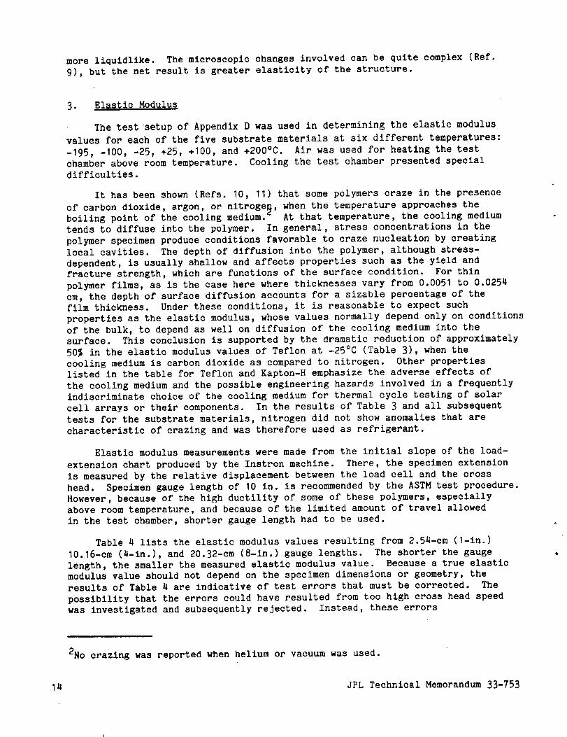
3. Elasti c Modulus

The test setup of Appendix D was used in determining the elastic modulus

values for each of the five substrate materials at six different temperatures:

-195, -100, -25, +25, +100, and +200°C. Air was used for heating the test

chamber above room temperature. Cooling the test chamber presented special

difficulties.

It has been shown (Refs. 10, 11) that some polymers craze in the presence

of carbon dioxide, argon, or nitrogen, when the temperature approaches the

boiling point off the cooling medium. _ At that temperature, the cooling medium

tends to diffuse into the polymer. In general, stress concentrations in the

polymer specimen produce conditions favorable to craze nucleation by creating

local cavities. The depth off diffusion into the polymer, although stress-

dependent, is usually shallow and affects properties such as the yield and

fracture strength, which are functions of the surface condition. For thin

polymer films, as is the case here where thicknesses vary from 0.0051 to 0.0254

cm, the depth of surface diffusion accounts for a sizable percentage off thefilm thickness. Under these conditions, it is reasonable to expect such

properties as the elastic modulus, whose values normally depend only on conditions

of the bulk, to depend as well on diffusion of the cooling medium into thesurface. This conclusion is supported by the dramatic reduction of approximately

50% in the elastic modulus values of Teflon at -25°C (Table 3), when the

cooling medium is carbon dioxide as compared to nitrogen. Other properties

listed in the table for Teflon and Kapton-H emphasize the adverse effects of

the cooling medium and the possible engineering hazards involved in a frequently

indiscriminate choice of the cooling medium for thermal cycle testing of solar

cell arrays or their components. In the results of Table 3 and all subsequent

tests for the substrate materials, nitrogen did not show anomalies that are

characteristic of crazing and was therefore used as refrigerant.

Elastic modulus measurements were made from the initial slope of the load-

extension chart produced by the Instron machine. There, the specimen extension

is measured by the relative displacement between the load cell and the cross

head. Specimen gauge length of 10 in. is recommended by the ASTM test procedure.

However, because of the high ductility of some of these polymers, especially

above room temperature, and because of the limited amount of travel allowed

in the test chamber, shorter gauge length had to be used.

Table 4 lists the elastic modulus values resulting from 2.54-cm (l-in.)

I0.16-cm (4-in.), and 20.32-cm (8-in.) gauge lengths. The shorter the gauge

length, the smaller the measured elastic modulus value. Because a true elasticmodulus value should not depend on the specimen dimensions or geometry, the

results of Table 4 are indicative of test errors that must be corrected. The

possibility that the errors could have resulted from too high cross head speed

was investigated and subsequently rejected. Instead, these errors

2No crazing was reported when helium or vacuum was used.


are believed to have resulted from a combination of (I) extensions in the gripand linkages of parts of the machine near the cross head, and (2) additionalnonuniform extension and possible slippage of the wrapped-around portion of thespecimen. Both effects contribute to greater errors for shorter specimens.

A correction to these errors was implemented by making use of the photo-graphic technique for the longitudinal strain measurements. As in the case forPoisson's ratio measurements, strains were computed from the longitudinaldeformations of a central portion of the specimen, away from the ends andexcluding their influence. Correction factors were computedby comparing theextension obtained from the displacement between the cross head and load cell,with the extension determined from photographs of the fiducial patterns. Thecorrection factors were computed at various temperatures and applied to thecorresponding results presented below.

A partial check was madeat room temperature by deriving the correctionsby a different approach. This latter approach is based on the premise that thetrue elastic modulus should be independent of the specimengauge length. Thus,if the measured "apparent" elastic modulus values are plotted against the gaugelength, as shownin Fig. 17, the "true" elastic modulus should be given by allne parallel to the gauge length axis and asymptotic to the curves at thegreater gauge length. This is true because greater errors are associated withshorter specimens. The corrected elastic moduli for room temperature resultingfrom the first approach and based upon extrapolation of the curves are comparedin Fig. 17. The corrected elastic moduli obtained by the two approaches are inrelatively good agreement.

In Tables 5 through 9, the measured and corrected values of elastic moduliare given for each of the five substrate materials at various temperatures forthe machine and the transverse direction of the specimens. The differencebetween the machine and transverse direction properties is indicative of thedegree of orthotropy of these polymers. The Mica Ply PG-402composite exhibitedthe greatest orthotropy of all the five materials tested. The transverse(fill) direction moduli for the Mica Ply are consistently about 75%of those inthe machine (warp) direction.

The temperature-dependence of the elastic modulus values is depicted inFigs. 18 and 19. The rate of change of these moduli with temperature variedgreatly for each material at different temperatures. In addition, Kapton-Hshowedsomedegree of irregularity at room temperature. These irregularitiesare characteristic of the behavior of the mechanical properties of long-chainpolymers (Ref. 8). They result from many types of transitions that can occurat different temperatures, including crystal melting, first-order crystallinetransitions, glass transitions, and secondary glass trans±tions.

4. Stress-Strgin B_avior, Yield Stress, and Fracture Strength

The stress-strain curves 3 up to fracture were determined for each of the

five materials at each of the six temperatures, namely -195, -100, -25, +25,

3Effects of strain rate and time on the creep and viscous flow when loads

are sustained for long times are not considered.


+100 and +200°C. Many of the special procedures and treatments discussed in

the previous two sections and in the appendixes were used here. Typical

tensile stress-strain curves at each of the test temperatures are shown in

Figs. 20 through 24 for Kapton-H, Kapton-F, Teflon, Tedlar, and Mica Ply PG-

402. The significance of these curves is mainly qualitative, showing trends

and characteristics of the material behavior under stress and temperature and

thus providing important design information.

Depending on the temperature and material, the initial linear elastic region

constituted from 0 to 100% of the total range to failure. For example, Teflon

and Tedlar (Figs. 22 and 23) behaved completely inelastically above I00°C, but

almost completely elastically and linearly near -195°C. Except for a limited

initial linearity, Kapton-H and Kapton-F (Figs. 20 and 21) tend to behave

markedly nonlinearly under loads at almost all temperatures within the range in

question. Mica Ply PG-402 on the other hand, responded linearly to loads at all

temperatures investigated because of the fiberglass reinforcement (Fig. 24).

Yielding in polymeric materials may take place by various mechanisms.

These include slipping between molecules or chains of molecules. Molecular

bonds may be temporarily broken and then reformed, or they may be permanently

broken. Friction, interlocking between particles, or fragmentation of particles

are possible. The question as to which of these mechanisms or combination of

mechanisms will actually take place depends upon, among other things, the

chemical composition, temperature, history of loading, and degree of crystallinity.

Accordingly, yielding may occur on a continuous and gradual basis, as is the

case with Kapton-H and Kapton-F at all temperatures investigated (Figs. 20 and

21). By contrast, yielding may occur at a definite stress level as exhibited

by Teflon and Tedlar at temperatures below +25°C (Figs. 22 and 23) and by Mica

Ply PG-402 (Fig. 24) at almost all temperatures. Here again, the absence of a

definite yield point in Tedlar and Teflon above +25°C and the presence of a

rather distinguishable one below that temperature indicate a strong association

with the same transformation revealed in the data on the thermal coefficient of

expansion (Fig. 15).

In testing of the five materials, a 3% offset yield stress was used to

define the yield point when a distinguishable yield point was not present.

While Figs. 20 through 24 represent the stress-strain curves for selected, but

typical, single test specimens, Figs. 25 and 26 depict the variation of the

statistical average yield stress of all specimens as temperature is changed

from -200 to +200°C. As may be expected, higher yield stresses are associated

with lower temperatures.

There are other very important design quantities such as the fracture

stress and strain that can be derived from the stress-strain behavior. Because

fracture failures in general are very sensitive to the presence of local

imperfections and the magnitude of the stress concentration at imperfections,

the fracture strength can be meaningful only in a statistical sense. This is

especially true for a brittle material like the Mica Ply PG-402 at nearly all

temperatures (Figs. 27 and 28). The specially designed cutting procedure of

Appendix E was intended to minimize the presence of edge imperfection and

stress raiser as much as possible. The results evidenced by the microscopic

examination of these edges (Appendix E) were smooth and relatively free from

imperfection except in the case of Mica Ply PG-402. This explains the reason

for the greater deviation from the average values in the case of Mica Ply


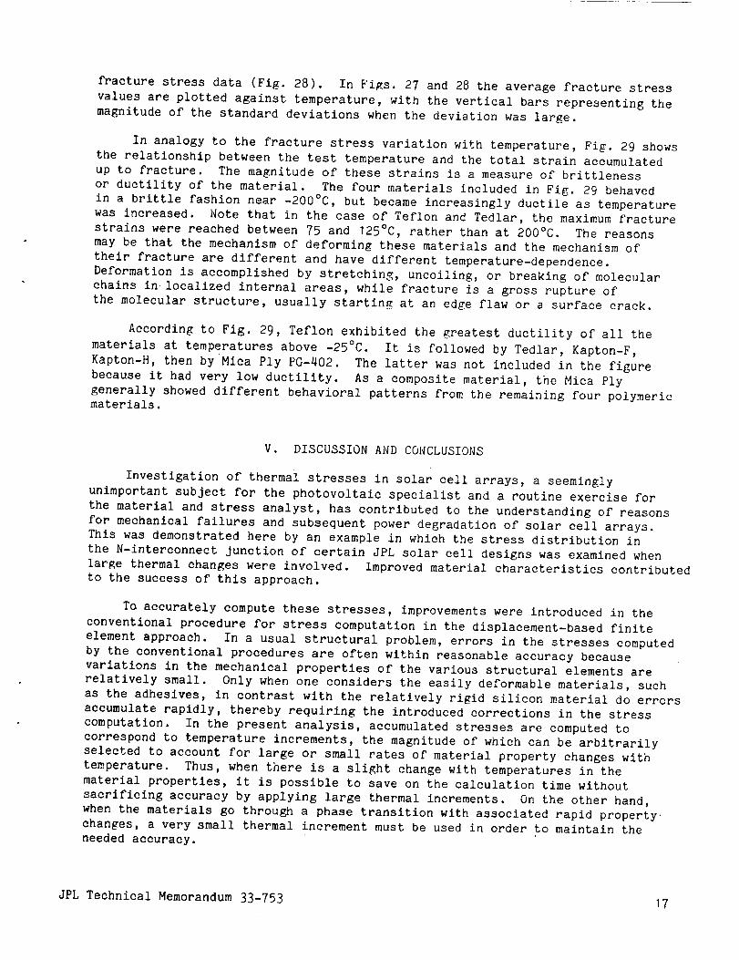
fracture stress data (Fig. 28). In Fins. 27 and 28 the average fracture stressvalues are plotted against temperature, with the vertical bars representing themagnitude of the standard deviations whenthe deviation was large.

In analogy to the fracture stress variation with temperature, Fig. 29 showsthe relationship between the test temperature and the total strain accumulatedup to fracture. The magnitude of these strains is a measureof brittlenessor ductility of the material. The four materials included in Fig. 29 behavedin a brittle fashion near -200°C, but becameincreasingly ductile as temperaturewas increased. Note that in the case of Teflon and Tedlar, the maximumfracturestrains were reached between 75 and 125°C, rather than at 200°C. The reasonsmaybe that the mechanismof deforming these materials and the mechanismoftheir fracture are different and have different temperature-dependence.Deformation is accomplished by stretching, uncoiling, or breaking of molecularchains in localized internal areas, while fracture is a gross rupture ofthe molecular structure, usually startin_ at an edge flaw or a surface crack.

According to Fig. 29, Teflon exhibited the greatest ductility of all thematerials at temperatures above -25°C. It is followed by Tedlar, Kapton-F,Kapton-H, then by Mica Ply PG-402. The latter wasnot included in the figurebecause it had very low ductility. As a composite material, the Mica Plygenerally showeddifferent behavioral patterns from the remaining four polymericmaterials.

V. DISCUSSIONANDCONCLUSIONS

Investigation of thermal stresses in solar cell arrays, a seeminglyunimportant subject for the photovoltaic specialist and a routine exercise for

the material and stress analyst, has contributed to the understanding of reasons

for mechanical failures and subsequent power degradation of solar cell arrays.

This was demonstrated here by an example in which the stress distribution in

the N-interconnect junction of certain JPL solar cell designs was examined when

large thermal changes were involved. Improved material characteristics contributed

to the success of this approach.

To accurately compute these stresses, improvements were introduced in the

conventional procedure for stress computation in the displacement-based finite

element approach. In a usual structural problem, errors in the stresses computed

by the conventional procedures are often within reasonable accuracy because

variations in the mechanical properties of the various structural elements are

relatively small. Only when one considers the easily deformable materials, such

as the adhesives, in contrast with the relatively rigid silicon material do errors

accumulate rapidly, thereby requiring the introduced corrections in the stress

computation. In the present analysis, accumulated stresses are computed to

correspond to temperature increments, the magnitude of which can be arbitrarily

selected to account for large or small rates of material property changes with

temperature. Thus, when there is a slight change with temperatures in the

material properties, it is possible to save on the calculation time without

sacrificing accuracy by applying large thermal increments. On the other hand,

when the materials go through a phase transition with associated rapid property

changes, a very small thermal increment must be used in order to maintain the

needed accuracy.


In any case, the computedstresses have additional significance when

interpreted in terms of a valid failure criterion. Here again, because of the

wide range of behavior of materials involved in the composite solar cell array,

it was necessary to provide the solar cell designer with more flexibility in

selecting the failure criterion that best describes the failure mode of each

material and temperature. The most general criterion covering a wide range of

ductile and brittle failure modes is the generalized Von Mises criterion

(Section III). It is particularly suitable for predicting failures in the

silicon material and adhesives below their glass transition temperature.

The final results presented in Table 2 combine effects of both the stress

corrections and the more accurate failure criteria. These are marked with

asterisks and are associated with either R I or R_. When compared with thecorresponding failure ratios R based on the origlnal version of Ref. 2, the

recommended ratios are found to be from 10 to 400% greater in absolute value

over R. However, the distribution of areas of relative stress concentration

and therefore the order of failure pattern remained unchanged regardless of

whether R, RI, or R2 was used. 1_qis is a peculiarity of the current example

and should not be expected as a general rule.

None of the above stress and failure analyses could be performed without a

good understanding and a reasonably accurate description of how certain key

properties of the solar cell materials change with temperature. For this

purpose, original work was carried out to identify the temperature-dependence

of selected materials of importance to the design of lightweight solar cell

arrays. They are the microsheet-0211 glass material for solar cell filter,

along with five substrate materials: Kapton-H, Kapton-F, Teflon, Tedlar and Mica

Ply PG-402. The temperature-dependence of the coefficient of thermal expansion,

elastic moduli, Polsson's ratio, strain and stress behavior of these materials

up to failure were determined. The properties were determined to different

levels of accuracy, depending on the composition of the individual material,

its stability in thermal environment, and the suitability of the employed test

technique. Properties of the microsheet-0211 glass material were relatively

well-behaved. On the other hand, properties of the Mica Ply PG-402 were rather

ill-behaved, primarily because it is a two-phase material in which the fibers

are not adequately stabilized to achieve consistent strength.

Most of the polymeric materials for the substrate showed strong, and occa-

sionally abrupt, changes with temperature. These result from many types of

phase transitions that can take place at different temperatures. Crystal melting,

first-order crystalline transitions, glass transitions, and secondary glass

transitions are possible causes. For the purpose of the present work, it is

not as important to identify which of these transitions actually took place

as it is to determine their net effect, whenever possible. A full investigation

of this subject was not attempted here because it requires much more elaborate

test techniques and greater cost. However, several of these effects were observed

and recorded in connection with a number of the material properties in question.

W_en thermal cycling tests of solar cell arrays are performed, a judicious

selection of the cooling medium is of prime importance. As was pointed out in

Section IV-B-3, certain refrigerants tend to easily diffuse into certain

polymers when their boiling point is reached. If this occurs, anomalous

effects and premature failures can result. Unless this is known, erroneous

results may go unnoticed.


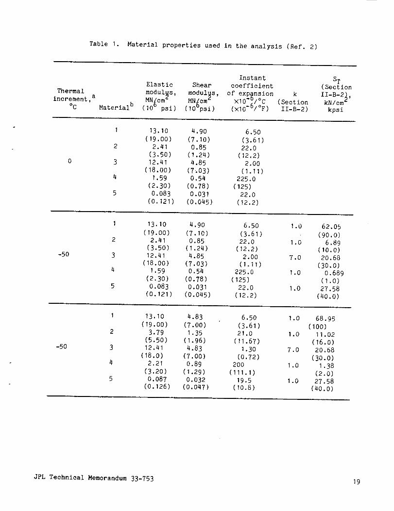
Table I. Material properties used in the analysis (Ref. 2)

Thermalincrement, a

oC

InstantElastic Shear coefficientmodulus modulus of expansion kMN_cm2 ' MN_cm2 ' ×I0-3/°C {Section

Material b (10 psi) (10_psi) (XIO-6/°F) II-B-2)

ST(SectionII-B-2_,kN/cm

kpsi

I 13.10 4.90 6.50

(19.00) (7.10) {3.61)

2 2.41 0.85 22.0

(3.50) {1.24) (12.2)

3 12.41 4.85 2.00

{18.00) (7_03) (1.11)

4 1.59 0.54 225.0

{2.30) {0.78) (125)

5 0.083 0.031 22.0

(0.121) {0.045) {12.2)

-5O

I 13.10 4.90 6.50

(19.00) (7.10) (3.61)2 2.41 0.85 22.0

{3.50) {1.24) (12.2)

3 12.41 4.85 2.00

(18.oo) (7.03) {1.11)4 1.59 0.54 225.0

(2.30) (0.78) (125)5 0.083 0.031 22.0

(0.121) (0.045) (12.2)

1.0

1.0

7.0

1.0

1.0

62.05

(90.0)

6.89(1o.o)

20.68

(30.0)0.689

(1.0)27.58

(40.0)

-5O

I 13.10 4.83 6.50

(19.00) (7.00) (3.61)

2 3.79 1.35 21.0

(5.50) (1.96) (11.67)

3 12.41 4.83 1.30

(18.0) (7.00) (0.72)

4 2.21 0.89 200

(3.20) (1.29) (111.1)

5 0.087 0.032 19.5

(o.126) (0.047) (1o.8)

1.0

1.0

7.0

1.0

1.0

68.95

(100)

11.02

(16.0)

20.68

(30.0)

1.38

(2.0)27.58

(40.0)


Table I (contd)

Thermalincrement,

oC

aMaterial b

Instant STElastic Shear coefficient (Sectionmodul_s, modul_s, of expansion, k II-B-2_,MN_cm MN_cm_ ×I0-_I°C (Section kNlcm_

(10v psi) (10v psi) (×I0 -°/°F) II-B-2) kpsi

-5O

I 13.03 4.76 6.50 1.0 89.63(18.9) (6.90) (3.61) (130)

2 4.48 1.60 18.0 1.0 13.79

(6.50) (2.32) (10.0) (20.0)

3 12.41 4.81 0.20 7.0 20.68

(18.0) (6.98) (0.11) (30.0)

4 1.38 0.62 110. 1.5 3.10

(2.00) (0.90) (61.11) (4.5)

5 0.092 0.034 16.5 1.0 27.58

(0.134) (0.050) (9.17) (40.0)

-35

I 12.96 4.76 6.50 1.0 110.3

(18.8) (6.90) (3.61) (160)

2 4.83 1.73 16.0 1.0 17.24

(7.00) (2.51) (8.89) (25.0)

3 12.4i 4.81 -0.90 7.0 20.68

(18.0) (6.97) (-0.5) (30.0)

4 1.03 .469 30.0 5.0 4.14

(1.50) (0.68) (16.67) (6.00)

5 0.099 0.037 11.0 1.0 27.58

(0.143) (0.054) (6.11) (40.0)

aFirst zero thermal increment is necessary for initialization only. Its

properties are arbitrary since it produces no stresses.

bMaterial type I = Kovar, 2 = solder, 3 = silicon, 4 : RTV-560 adhesive,

5 = equivalent solid aluminum substrate.


Table 2. Sugary of failure ratios in N-interconnect junction

Fail-Location designated in Fig. 6b

Config- ureuration ratio

A I A2 A 3 A4 A 5 A6 A 7 A8 A9 AI 0

R I

R2

R

0.12" 0.50* 0.30* 0.28* 2.3* 0.62* 0.75*

0.10 0.44 0.275 0.26 2.0 0.57 0.65

0.10 0.27 0.275 0.19 2.0 0.25 0.40

1.2' 0.46* 0.28*

0.31 0.33 0.30

R I

R2

R

0.33* 0.31" 0.31" 0.26* 1.8" 0.61" 0.64*

0.03 0.28 0.275 0.25 1.6 0.55 0.59

0.03 0.125 0.275 0.105 1.6 0.32 0.48

m -- --

1.5' 0.79* 0.56*

0.38 0.12 0.22


Table 3. Effects of testing in carbon dioxide and nitrogen

(2.54-em gauge length, machine direction, -25°C)

Material

Measured 3%

elastic yield Fracture Fracture

modulus, stress, stress, strain,

GN/m 2 (psi) MN/m 2 (psi) MN/m 2 (psi) % Refrigerant

Teflon

Teflon

Kapton-H

Kapton-H

0.41 22.48 44.13 505

(59,600) (3,260) (6,400)

0.89 18.96 31.23 303

(129,290) (2,750) (4,530)

1.34 55.85 111.35 66

(194,890) (8,100) (16,150)

2.04 71.29 161.96 96

(295,710) (10,340) (23,490)

CO 2

N2

CO 2

N2


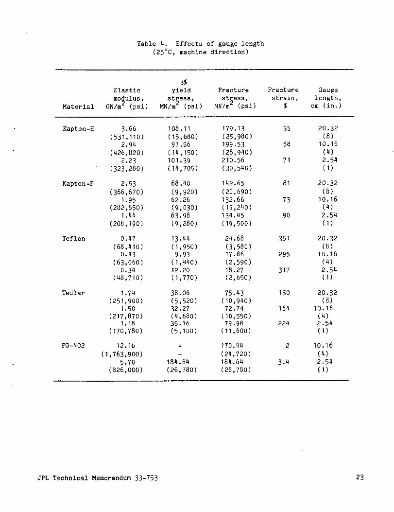
Table 4. Effects of gauge length(25°C, machine direction)

Material

Elastic

modulus,GN/m (psi)

3%yield Fracture

stress, stress,

MN/m 2 (psi) MN/m 2 (psi)

Fracture

strain,

%

Gauge

length,

cm (in.)

Kapton-H

Kapton-F

Teflon

Tedlar

PG-402

3.66 108.11 179.13 35 20.32

(531,110) (15,680) (25,980) (8)

2.94 97.56 199.53 58 10.16

(426,820) (14,150) (28,940) (4)

2.23 101.39 210.56 71 2.54

(323,280) (14,705) (30,540) (I)

2.53 68.40 142.65 81 20.32

(366,670) (9,920) (20,690) (8)

1.95 62.26 132.66 73 10.16

(282,850) (9,030) (19,240) (4)

1.44 63.98 134.45 90 2.54

(208,190) (9,280) (19,500) (I)

0.47

(68,410)

0.43

(63,060)

0.34

(48,710)

13.44 24.68

(1,950) (3,580)

9.93 17.86

(1,440) (2,590)

12.20 18.27

(1,770) (2,650)

351

295

317

20.32

(8)10.16

(4)

2.54

(I)

1.74 38.06 75.43 150 20.32

(251,900) (5,520) (10,940) (8)

1.50 32.27 72.74 164 10.16

(217,870) (4,680) (10,550) (4)

1.18 35.16 79.98 224 2.54

(170,780) (5,100) (11,600) (I)

12.16 - 170.44 2

(1,763,900) - (24,720)

5.70 184.64 184.64 3.4

(826,000) (26,780) (26,780)

10.16

(4)2.54

(I)


Table 5. Summarydata, Kapton-H(0.00762 cm, 0.003 in. thick; 2.54 cm, 1.0 in. gauge length)

Testtemp-

erature,°C

Measured Corrected 3%elastic elastic yield Fracturemodulus, modulus, stress, stress, FractureGN/m- GN/m_ MN/m- MN/m_ strain,(psi) (psi) (psi) (psi) %

Specimendirection

2O0

2OO

100

100

25

25

-25

-25

-100

-100

-195

-195

1.206

(175,050)1.213

(176,040)

2.093(3O3,8OO)

1.811

(262,820)

2.227

(323,280)

2.218

(321 970)

3.025

(439,040)

3.009

(436,710)

3.678

(533,830)

3.648

(529,430)

4.346

(630,730)

4.168

(604,980)

1.218

(176,840)

1,225

(177,800)3.621

(526,330)

3.133

(454,680)

3.585

(520,500)

3.571

(518,370)

4.507

(654,170)

4.483

(650,7O0)

4.781

(693,980)

4.742

(688,300)

5.215

(756,900)

5.002

(735,300)

8O

11

74

(10

93

(13

79

(11

101

(14

98

(14

118

(17

116

(16

174

(25159

(23

234

(33

225

(32

•96 125.98 83 Machine

,750) (18,285)

•34 120.40 79 Transverse

,790) (17,475)

•77 161.78 65 Machine

,510) (23,480)

.44 153.85 74 Transverse

,530) (22,330)

.32 210.42 71 Machine

,705) (30,540)


,360) (30,200)

•30 237.08 54 Machine

,170) (34,410)

.58 232.33 58 Transverse

,920) (33,720)

.18 313.01 52 Machine

,280) (45,430)


,110) (39,230)

.05 350.49 36 Machine

,970) (50,870)


,800) (46,030)


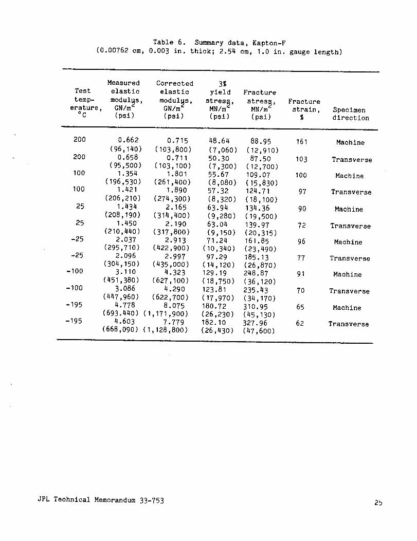
Table 6. Summarydata, Kapton-F(0.00762 cm, 0.003 in. thick; 2.54 cm, 1.0 in. gauge length)

Testtemp-

erature,oC

Measured Corrected 3%elastic elastic yield Fracturemodul_s, modulss, stress, stress, FractureGN/m GN/m- MN/m MN/m_ strain,(psi) (psi) (psi) (psi) %

Specimendirection

200

200

100

100

25

25

-25

-25

-100

-100

-195

-195

0.662 0.715 48.64 88.95 161(96,140) (103,800) (7,060) (12,910)

0.658 0.711 50.30 87.50 103(95,500) (103,100) (7,300) (12,700)

1.354 1.801 55.67 I09.07 100(196,530) (261,400) (8,080) (15,830)

1.421 1.890 57.32 124.71 97(206,210) (274,300) (8,320) (18,100)

1.434 2.165 63.94 134.36 90(208,190) (314,400) (9,280) (19,500)

1.450 2.190 63.04 139.97 72(210,440) (317,800) (9,150) (20,315)

2.037 2.913 71.24 161.85 96(295,710) (422,900) (10,340) (23,490)

2.096 2.997 97.29 185.13 77(304,150) (435,000) (14,120) (26,870)

3.110 4.323 129.19 248.87 91(451,380) (627,100) (18,750) (36,120)

3.086 4.290 123.81 235.43 70(447,960) (622,700) (17,970) (34,170)

4.778 8.075 180.72 310.95 65(693.440) (1,171,900) (26,230) (45,130)

4.603 7.779 182.10 327.96 62(668,090) (1,128,800) (26,430) (47,600)

Machine

Transverse

Machine

Transverse

Machine

Transverse

Machine

Transverse

Machine

Transverse

Machine

Transverse


Table 7. Summarydata, Teflon(0.0127 cm, 0.005 in. thick; 2.54 cm, 1.0 in. gauge length)

Testtemp-

erature,°C

Measured Corrected 3%elastic elastic yield Fracturemodul_s, modul_s, stress, stress, Fracture

GN/m- GN/m- MN/m- MN/m- strain,(psi) (psi) (psi) (psi) %

Specimendirection

200 16.71 19.22 1.21(2,425) (2,790) (175)

200 15.78 18.15 1.10(2,290) (2,630) (160)

100 55.64 96.81 3.55(8,075) (14,050) (515)

100 51.05 88.83 2.62(7,410) (12,900) (380)

25 335.51 486.49 12.20(48,710) (70,600) (1,770)

25 346.50 502.43 11.51(50,290) (72,900) (1,670)

-25 890.81 1042.25 18.95(129,290) (150,000) (2,750)

-25 917.82 1073.85 18.53(133,210) (155,900) (2,690)

-100 1982.8 2478.5 69.45(287,780) (348,600) (10,080)

-100 1974.0 2467.5 68.07(286,500) (358,100) (9,880)

-195 3290.5 6679.7 98.18(477,570) (969,500) (14,250)

-195 3553.7 7214.0 114.93(515,780) (1,047,000) (16,680)

3.48(5O5)

1.93

(280)

12.33

(1,790)

8.34

(1 210)18,26

(2,650)17,36

(2,520)

31,21

(4,530)

32.73

(4,750)

67.25

(9,76O)

66.28

(9,620)

95.01

(13,790)

109.83

(15,940)

378 Machine

298 Transverse

399 Machine

324 Transverse

317 Machine

306 Transverse

303 Machine

314 Transverse

132 Machine

81 Transverse

15 Machine

15 Transverse


Table 8. Summarydata, Tedlar(0.0051 cm, 0.002 in. thick; 2.54 cm, 1.0 in. gauge length)

Testtemp-

erature,oC

Measured Corrected 3%elastic elastic yield Fracturemodulus, modu½us, stress, stre_s, FractureGN/m2 GN/m MN/m2 MN/m strain,(psi) (psi) (psi) (psi) %

Specimendirection

150

150

100

IO0

25

25

-25

-25

-100

-1OO

-195

-195

30.66 34.95 3.07 20.88 238(4,450) (5,070) (445) (3,030)39.55 45.09 2.84 18.64 220(5,740) (6,540) (412) (2,705)

114.20 121.05 7.72 38.72 259(16,575) (17,570) (1,120) (5,620)103.97 110.21 6.20 48.09 224(15,090) (16,000) (900) (6,980)

1176.7 2388.7 35.14 79.92 224(170,780) (348,300) (5,100) (11,600)1152.5 2339.6 32.93 75.24 161(167,270) (339,560) (4,780) (10,920)1826.7 4146.6 75.51 110.38 129(265,130) (601,530) (10,960) (16,020)1900.0 4313.0 70.14 128.50 102(275,760) (625,980) (10,180) (18,650)3895.8 8103.3 148.76 166.46 38(565,430) (1,174,980) (21,590) (24,160)4102.7 8533.6 154.89 197.40 47(595,450) (1,237,340) (22,480) (28,650)4922.4 9401.8 213.18 245.28 7.6(714,430) (1,364,550) (30,940) (35,600)4811.1 9189.2 150.89 192.23 7.8(698,280) (1,333,700) (21,900) (27,900)

Machine

Transverse

Machine

Transverse

Machine

Transverse

Machine

Transverse

Machine

Transverse

Machine

Transverse


Table 9. Summarydata, PG-402(0.00635 cm, 0.0025 in. thick; 2.54 cm, 1.0 in. gauge length)

TestTemp-

erature,°C

Measured Corrected 3%elastic elastic yield Fracturemodulus, modulus, stress, stress, Fracture

GN/m2 GN/m2 MN/m_ MN/m strain,(psi) (psi) (psi) (psi) %

Specimendirection

200 5.428 14.547(787,800) (2,111,300)

200 3.782 10.136(548,870) (1,471,000)

100 5.832 15.222(846,380) (2,209,000)

100 4.342 11.333(630,220) (1,644,900)

25 5.691 19.748(826,000) (2,866,300)

25 4.335 15.042(629,110) (2,183,000)

-25 5.916 19.996(858,640) (2,902,200)

-25 4.372 14.777(634,580) (2,144,900)

-100 6.220 24.071(902,710) (3,493,500)

-100 5.129 19.849(744,360) (2,880,700)

-195 7.431 23.036(1,078,570) (3,343,600)

-195 5.419 16.799(786,480) (2,438,100)

160.47(23,290)I03.56

(15,030)151.10

(21,930)80.61

(11,700)184.51

(26 780)

117.68

(17,080)

171.35

(24.870)

108.86

(15,800)

199.33(28,930)

104.25

(15,130)181.41

(26,330)131.81

(19,130)

160.47 3.2 Warp

(23,290)

103.56 3.4 Fill

(15,030)

151.10 2.7 Warp(21,930)80.61 1.7 Flll

(11,700)

184.51 3.4 Warp

(26,780)

117.68 2.7 Fill

(17,080)

201.81 3.7 Warp

(29,290)

131.12 3.8 Fill

(19,030)

312.74 6.7 Warp

(45,390)

227.85 6.7 Fill

(33,070)

381.22 7.6 Warp

(55,330)

241.91 6.3 Fill

(35,11o)


SOLDERRESI!

SILICON SOLARCELL

P-I (2 cm X 2 cm X 0.036 cm)

SILICONE ADHESIVE

,CELLTO COVERSLI DE BOND, --_ _ N INTERCONNECTOR

0.051 cm REF.-_ _F-GLASS _ Ol

I ' _,_ '" I _-, 1:i,____:___"_2.................... :_ ..... 1 L-- 0.127 ¢mo.o,o<:-.-1 L--RADIUS TYP 2 cm X ? cm X 0.036 cm ,,L'F-0.020cm RADIUS TYP

//

/

DIELECTRIC INSULATION --"0.013 cm FIBERGLASSEPOXY

//

VI

HONEYCOMBSUB1.2/cm CORE (VENTEDI0.013 cm THICK SKINBOTH SURFACES

Fig. I. Solar cell configuration 1


CTOR

SOLDERRESIST

P-INTERCONNECTORN-INTERCONNECTOR

SILICON SOLARCELL

12cm X 2 cmX 0,0BOcm)

SILICONE ADHESIVE

(CELLTO COVERSLIDE BONDI"-_

/_ P [NTERCONNECTOR _ ,_--- N ,NTERCONNECTOR

0"051 cm REF-P 1 _ "_\ "_

.// /--- GLASS 'P1 _ 0.0! cm MIN _'_J([._

Jj L__ " ......... '_.................. J L--

/""/I SIUCON SOLAR CELL _//,.,./1 _ 0.046 cm RH} .US Typ it_.{,. J 2 cm X 2cm X O.(TJ6cm _L,--F- n_" _..*'_'_.._..-i//////// ............. X/////,/_, _" w_// ............................ Y///'//_

r

Ii /

SILICONE ADHESIVE -/ /

0.013cm FIBERGLASSEPOXY

/

//

/

HONEYCOMBSUBITRA_

1.27 cm CORE(VENTEDI0.013 cm THICK SKINBOTHSURFACES

Fig. 2. Solar cell configuration 2

3O JPL Technical Memorandum 33-753

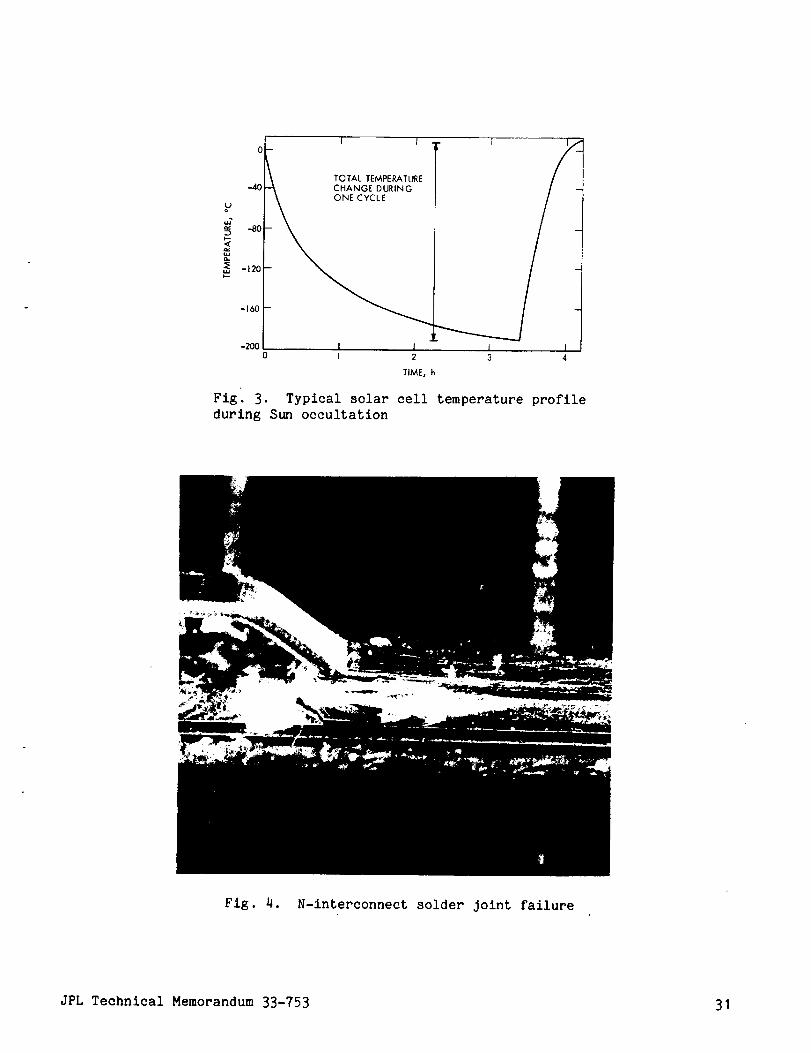
o

-4o

-80.,,t"

-120I--

-160

-200

I I

TOTAL TEMPERATURE

CHANGE DURING

1 2

TIME, h

J I3 4

Fig 3. Typical solar cell temperature profile

during Sun occultation

Flg. 4. N-interconnect solder joint failure


f_

KOVAIR_N-INIERCONNECT

_SOLDER

SILICON

ADHESIVE

SUBSTRATE

Fig. 5. Portion of finite element model

of N-interconnect junction


(c,) -.- (0.0508 cm

0.020 in.)

I

0.127cm _0.O_i27cm

(0.050 in.)/ (0°005 in.) 0.0762 cm Rl P-SEND io.o3o_o._t

0.381 crnc (0.150 in.)

'FF. -_o ,_cm o0.381 cm TYP _ .381 cm l 32.5 ° TYP

--_,-(o.15o _n./ o.127cmI..,-ro.,5o ;o.)-_TYP _ (0.05 in.) (0.05 in.) TYP

1.016 cm (0 40 in.

B (CONFIGURATION 2)

DETAIL A

A (CONFIGURATION l)

T-- 0.254 cm R i_'-'P'BEND\(0. i0in.)

0.127 cm "_YP_(0.050 in.) ]_

0.0127 _ b - 0.762 cm(0,,005 _n,) 10.25 cm (0.300 in.)

{0. IO0 in.) TYP

TYP DETAIL B

(b)

•_AL PAGE ISPOOR QUALI_

S CONFIGURATION I

._..... _. _. / F CONFIGURATION 2

A 3

Fig. 6. N-interconnect Junction: (a) two interconnectgeometries, (b) most stressed areas, leading to failures


8.0

6.0

_v\ _.ou.._oI,L P"111

o,,x, 2.0U

m

D"D-

- if,0"

I .OJ o...O.. O. O-

1_ o..Cr'O " O''O" _

0 I I I,-200 -100 0 100 200

TEMPERATUREs °C

Fig. 7. Instantaneous coefficient of expansion of

0211 glass as a function of temperature

75.84 J I I I>_ 74.46 [73.08

71.71F o_% 70.33 -£-o-_-o-O-a-_-.a..o_o_oo_u. Z" 68.95

o< o om 67.57 - O O -

66.19

64.81O

63.4362.05

_O El1 ELASTIC MODULUS COMPUTEDFROM THE FIRST BENDING FREQUENCY

-[7E2, ELASTIC MODULUS COMPUTED FROM-- THE SECOND BENDING FREQUENCY

I I I-200 -I00 0 100 200

TEMPERATUREt °C

II .0I0.810.6 _

10.4

110.2 _ "-

10.0

9.6 --

9.4 0

9.29.0

Fig. 8. Modulus of elasticity as a function of temperature for

0211 glass

_ 29.65

28.96

,v _o 28.61

-.r- 28.27

I I I _7

_o.O.o-.Oo-o-o--o.b_ - 4.3o_ .__

4.15 ._ "-

4.10I I I ,,',

-200 -1 O0 0 1O0 200

TEMPERATUREe °C

Fig. 9. Shear modulus as a function of temperature for

0211 glass


:L 0.24 A

_DO 0,20 jO0..0..0...0..0..0..0..0._ _ .0"

_ _-o-_r , ,-200 -100 0 1O0 200

TEMPERATURE, °C

Fig. 10. Poisson's ratio as a function of temperature

for 0211 glass

:_ 200

_.o¢./3

Z_ 15o,x,O 100

----_'0u '- 50

LIJ

Ou 0

I I I

iCk_ P _,,

I

I \

xyo

_ _o_o.O-_°_ \0...0 _ I

0

I.... I I-200 - 1O0 0 1O0 "

TEMPERATURE, °C

200


Tedlar vs temperature


7O

6O

_o5o

E4o

u_ 20U-L#J

0u 10

0

I I I

0 o

0 f "-'- _.,.p 0

o//o/Oo o

0 0 0 0-

/-c_

0

I i I ,

-200 -100 0 lO0 200

TEMPERATURE, °C


Kapton-F vs temperature

50

ov_ 40Z

_ 30o;_pu 20uJ 'O

_'- 10LL11LU

0 0U

I I' i

- o o..Oo o__O.O_o0

_ oo.OO-Oo oo/ o

I l I-200 -100 0 1O0 200

TEMPERATURE, °C

Fig. 13. Instantaneous coefficient of expansion of.

Kapton-H vs temperature


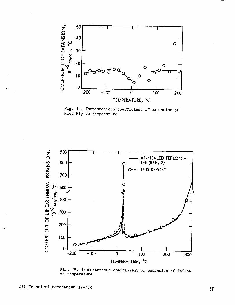
5O

o40Z

_P_30

0

I I I

I

0

i

?u 20 I_ 0 -

_)o F-I_°'°_°_%°" o -_-o--o--o10 0 --0 0

0I I I IU

-200 -I00 0 100 200

TEMPERATURE, °C


Mica Ply vs temperature

9OO

800Z

,x, 700

,.,,.I

400

_z?__o300

200ILl

1ooE

oU

I I I I

-- ANNEALED TEFLON -

- Q TFE (REF. 7) -

I O--- THIS REPORT

O"

-200 -100 0 100 200 300

TEMPERATURE, °C

Fig. 15. Instantaneous coefficient of expansion of Teflon

vs temperature


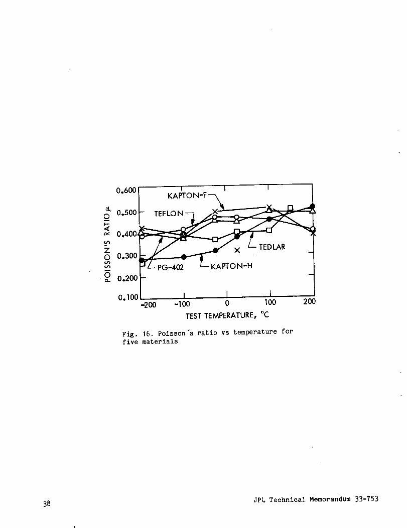
0.600

IKAPTO

TEF LO N

PG -402 KA PTO N-H

I I

TEDLAR

o. lOO I I I-200 -100 0 100

TEST TEMPERATURE., °C

2OO

Fig. 16. Poisson's ratio vs temperature forfive materials


6.0

5,o

__ 4.0

3.0

U

2.0

1.0

1 I I I I I

MICA PLY PG_

_ ls._ (is.17)*

/ 3.e_6(3.62)*• KAFrON-H

,,_ KAPTON-F_-/._ 2.0(2.34)* -

* VALUES IN PARENTHESES ARE COMPUTED

TEFLON 0.48 (0.48)*

0 J I I I I I0 5,0 10,0 15,0 20.0 25.0 30,0

GAUGE LENGTHt cm

16.0

14.0

12,0 _._,

10.0

U

8.0 _

6.0

4.0

Fig. 17. Elastic modulus variation with gauge length at 25°C: an

alternative approach to establish correction factor for gauge

length effect on modulus values


8.274--J

0

u _ 5.516

<_ 0

k-

u 2.758I.IJ

0U

TEFLON

TEDLAR

KAPTON-H

KA PTO N-f:

0 I-200 -100 0 100 200

TEMPERATUREt °C

Fig. 18. Corrected elastic modulus vs test temperature for

tensile loading (materials as marked)

27.576

i 2O.682

U_

la.788

O

u 6.894

I I I

MACHINE (WARP)

CTION

O -

- TRANSVERSE (FILL)

DIRECT ION

! I I-200 -100 0 100 200

4OOO

B

3000

U _

'2000

0

moo0 u

TEMPERATUREt °C

Flg. 19. Corrected elastic modulus vs test temperature for tensile

loading of PG-402 fiberglass composite


I co275-8r/_

_ iy_ -_5

• 2oo-

OF 1 ....I I I I 1 I0 10 20 30 40 50 60 70 80

STRA INt %

40,000 "_

20,000

0

Fig. 20. Typical tensile stress-strain curves for Kapton-H

(0.00762-cm, 0.O03-in. thick)

e_

_ 275.8

137.9

00

I I I

- , / "195°C-100

125

25

2___.2oo

V i , ,50 ,100 150

40,000 '_

i,a.i,v

20,000 _"'

Z

p-

0

STRAIN, %

Fig. 21. Typical tensile stress-strain curves for Kapton-F

(0.00762-cm, 0.O03-in. thick)


I I

110.3 "195°Ce_E

82.78

Ill,V

55,16

_Z 27.57

0

I I I

r_,._t -100

.25

25._..100

i 12000 100 200 300 400 500

STRAIN, %

16t000

12,000

80OO

40OO

0

Fig. 22. Typical tensile stress-strain curves for Teflon

(0.00762-cm, 0.003-in. thick)

.u

uJm_

ILl..Ju

t_

z

275.8 J I I I I

eq [j.195oC206.8 -100

137.9

68.95

0[ _1500 50 100 150 200 250

,40,OOO

30,000 i20, OOO

10,000 NZ

0

STRAIN, %

Fig. 23. Typical tensile stress-strain curves for Tedlar

(0.0051-cm, 0.O02-in. thick)


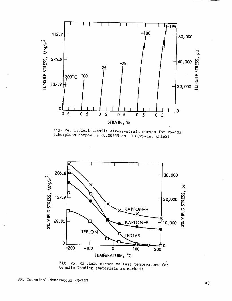
E

275.8I.u

1.1.1_.1

Z 137,9

I I ! ' "1 I I I

200oC 100

0 I I ' I

05 O5

-2525

I I I I

05 05

STRAIN, %

I I

-100

I 1-195

m

I I,, I I

05 05

60, 000

",7,o_

40,000 ..u'l.

I.--

I.i,,I._,J

Z20,000 "'

I.,,-

0

Fig. 24. Typical tensile stress-strain curves for PG-402

fiberglass composite (0.00635-cm, 0.0025-in. thick)

)<

206,8

I I I

30,000

-X - 8.

ID u_

137.9 - X - 20, 000 _"'

_X KAPTON-H ..a

\ ,,,_68.95 - 10, 000 o_

-200 -100 0 100 200

TEMPERATURE, °C

Fig. 25. 3% yield stress vs test temperature for

tensile loading (materials as marked)


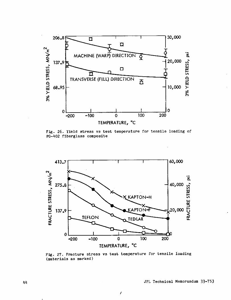
TRANSVERSE (FILL) DIRECTION

0

i5

I 1 I-200 -100 0 100 200

10,000

0

TEMPERATURE, °C

Fig. 26. Yield stress vs test temperature for tensile loading of

PG-402 fiberglass composite

413.7 1 I I I 60,000I

e_ X "

"_ 275.8 40,000

_. N-H

× _1 2

0-200 -100 0 100 200

TEMPERATURE, °C

Fig. 27. Fracture stress vs test temperature for tensile ioading

(materials as marked)


413.7__,_ I I I

m

60,000

20, 000

40,000

2 137.9

DIRECTIONI.I.

o I I I o-200 -100 0 100 200

TEMPERATURE, °C

n

i.,tJ

t-.

ELI

:DI.--U<

Fig. 28. Fracture stress vs test temperature for tensile loading

of PG-402 fiberglass composite

400 ¸

X_ 3OO

200ILl

F-U 100

u.. 0

-200 -100

I I

TEDLAR

KAPTON-F

KAPTON-H! i0 100 200

TEMPERATURE, °C

Fig. 29. Strain to fracture vs test temperature for

tensile loading


APPENDIX A

STRESS COMPUTATION IN DISPLACEMENT METHODS

FOR TWO-MATERIAL ELASTIC MEDIA

I. INTRODUCTION

The stress computation in displacement methods for the structures of two-

and three-dimensional continua is an important aspect of a systematic struc-

tural analysis. Once the displacements are computed at the nodes of a finite

element mesh covering the material volume of the structure, the problem of

stress computation at the nodes may be handled in various ways (Refs. 12-19).

For example, a usual procedure is to compute stresses from the conditions of

compatibility and constitutive relations (Ref. 12). In addition, various

schemes of stress averaging (Ref. 13), best fit strains (Ref. 14), and virtual

strains (Ref. 15) have been recommended. Stresses obtained by these procedures

do not necessarilysatisfy the conditions of force equilibrium, especially at

boundary points. Recently, an improvement upon these methods has been

suggested (Ref.16) in a computational procedure where equilibrium equations are

used at the nodes along with the principle of virtual displacements to establish

a local stress distribution. No constitutive relationships were used. In this

appendix a similar treatment is offered to improve upon the values of internal

stresses in continua having more than one material. The work was originally

motivated by the fact that when more than one material is involved in the fi-

nite element model, and when the stresses are computed on the basis of compatibility

and constitutive relations alone, severe violation of force equilibrium may

take place at the intermaterial boundary points. Stronger violation of equilibrium

conditions is associated with greater differences between the properties of

adjacent materials. The approach taken here is concerned with a generalizationof the method of best fit strain tensors (Ref. 14) for the stress computation

at intermaterial boundary points, so that compatibility, constitutive, and equi-

librium conditions are satisfied.

The method of best fit strain tensors was found convenient and economical.

It has been in use in several computer codes (Refs. 20-22) for elastic and

inelastic materials undergoing geometrically linear deformations. In the

following, the method is summarized; then a generalization of the method to

handle intermaterlal boundary points of two-material continua is presented, and

examples of results obtained are given. Again, the objective here is maintaining

accuracy while insuring equilibrium, compatibility and the satisfaction of the

constitutive relationship. Satisfying the constitutive relationship is especially

important when dealing with inelastic material behaviour.

II. THE METHOD OF BEST FIT STRAIN TENSORS

This method of stress computation is modular, not in mesh elements (i.e.,

finite elements) but in node sets. A node set associated with a node is

defined (Ref. 14) as the list of nodes coincident with the vertices of all mesh

elements meeting at that node. The set of nodal lines joining the node with

the other nodes listed in the nodal set is called the nodal line set. Numerical


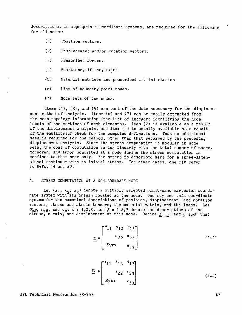
descriptions, in appropriate coordinate systems, are required for the followingfor all nodes:

(I) Position vectors.

(2) Displacement and/or rotation vectors.

(3) Prescribed forces.

(4) Reactions, if they exist.

(5) Material matrices and prescribed initial strains.

(6) List of boundary point nodes.

(7) Nodesets of the nodes.

Items (I), (3), and (5) are part of the data necessary for the displace-ment methodof analysis. Items (6) and (7) can be easily extracted fromthe meshtopology information (the list of integers identifying the nodelabels of the vertices of meshelements). Item (2) is available as a resultof the displacement analysis, and item (4) is usually available as a resultof the equilibrium check for the computeddeflections. Thus no additionaldata is required for the method, other than that required by the precedingdisplacement analysis. Since the stress computation is modular in nodesets, the cost of computation varies linearly with the total number of nodes.Moreover, any error committed at a node during the stress computation isconfined to that node only. The method is described here for a three-dimen-sional continuum with no initial stress. For other cases, one mayreferto Refs. 14 and 20.

A. STRESSCOMPUTATIONAT A NON-BOUNDARYNODE

Let (Xl, x2, x_) denote a suitably selected right-hand cartesian coordi-nate system with its-origin located at the node. Onemayuse this coordinatesystem for the numerical descriptions of position, displacement, and rotationvectors, stress and strain tensors, the material matrix, and the loads. Let_aB, _, and u_, _ = 1,2,3, and _ = 1,2,3 denote the descriptions of the

stress,-strain, and displacement at this node. Define _, _, and _ such that

_iI _12 e-li]Sym _3

(A-I)

Ell c12E_ : 'ZZ

L Sym c33J

(A-2)


T Uz u3 ]u_ = [u 1, , (A-3)

Also, let

-_ = ii' _22' °-12' _33' °-13' _23 '(A-4)

and

c T [c c Zc 2, c 2c 3, 2c ] (A-5)= 11' Z2' 1 33' 1 23 "

With the latter notation, the stress-strain relationship may be stated as

= D c. (A-6)

where D is the material matrix Note that D : DT and D is positive definite

Let m denote the total number of nodal lines in the nodal line set of the node.

Let pi denote the unit vector in the direction of the ith nodal line. with i

denoted as the relative displacement of the ith node in the node set relative

t_hthe node at the origin, and _l as the lineal strain in the direction of thei nodal line, we may write

.Ti _ i

= p _ p (A-7)u

where no sum is implied by the repetition of index i. For the strain along the

ith nodal line, one may also write

.Ti t i i

c _ p _u -c o , (A-_)

where _0i is the prescribed strain in the direction of the ith nodal line.

Instead of Eq. (A-8), it is possible to use a hlgher-order approximation (Ref.

23). However, if the mesh is sufficiently refined, there is no need for such a

scheme. By equatin_ the right-hand sides of Eqs. (A-7) and (A-8),

.T .TI i i i i

p Ep : p u - c o , (A-9)

or by means of the definitions in Eqs. (A-2) and (A-5),


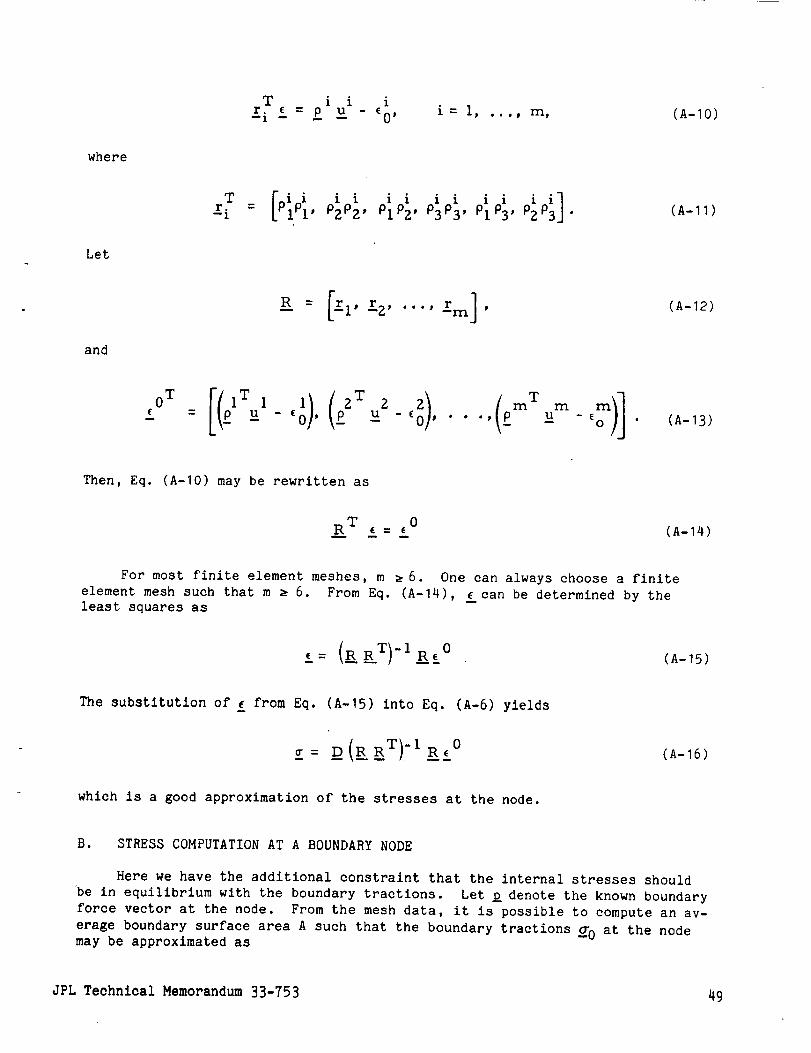
T i i i_ri i = _P u - _0' i = I, ..., rn, (A-IO)

where

T [ii i i ii ii ii ii3]_ri : PlPl, P2P2 , PlP2 , P3P3 , PlP3 , P2 p •(A-11)

Let

and

(A-12)

o. [(: ol)(_,'" 02) (:"I T 1 2 m mi = u - c , _u -_ , • .., u m)] (A-13)

Then, Eq. (A-IO) may be rewritten as

R_RT i= ! 0 (A-14)

For most finite element meshes, m m 6. One can always choose a finite

element mesh such that m m 6. From Eq. (A-14), ( can be determined by the

least squares as

,_: o (A-?5)

The substitution of ( from Eq. (A-15) into Eq. (A-6) yieldsm

__: _D(R_R_T)-iR_,_° (A-_6)

which is a good approximation of the stresses at the node.

B. STRESS COMPUTATION AT A BOUNDARY NODE

Here we have the additional constraint that the internal stresses should

be in equilibrium with the boundary tractions. Let _ denote the known boundary

force vector at the node. From the mesh data, it is possible to compute an av-

erage boundary surface area A such that the boundary tractions _0 at the nodemay be approximated as


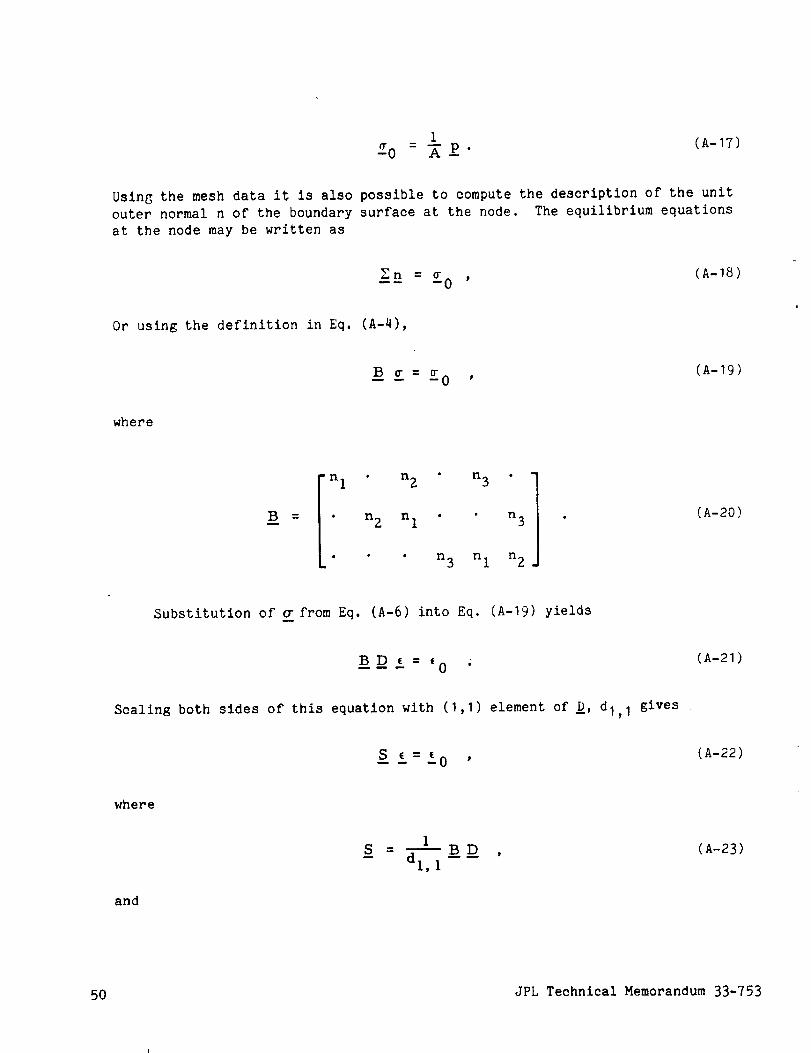
l-_0 = _ p " (A-17)

Using the mesh data it is also possible to compute the description of the unit

outer normal n of the boundary surface at the node. The equilibrium equations

at the node may be written as

Zn = _ (A-18)m_ m 0 P

Or using the definition in Eq. (A-4),

B o- -- o- 0 •

(A-19)

where

B ._w i!I.n3]n z n I • • n 3 •

. . n 3 n I n z

(A-20)

Substitution of @ from Eq. (A-6) into Eq. (A-19) yields

BD_=_0

(A-21)

Scaling both sides of this equation with (1,1) element of _, dl, I gives

S _ = _0 'n m

(A-22)

where

1S : _BD-- dl, 1 -- --

(A-23)

and


I (A-24)-0 dl, 1 -0 .

The strain-deflection equations of the nodal line set are as in Eq.

(A-14). Combining Eqs. (A-14) and (A-22),

E = , (A-25)

where ( may be solved by least squares asm

Z (A-26)

The substitution of _ from Eq. (A-26) into Eq. (A-6) yields the desired stresses•

Alternatively, from Eq. (A-22), one can solve for some of the components

of A in terms of the remaining components. Let i" and !", respectively,

denote the independent and the dependent components of _. The choice of _" canN

be made such that

= i' _' (A-27)

Calling the corresponding conformable partitions of _, _" and _", one obtains

= IS' , S"] .. (A-28)

Rewriting Eq. (A-22) with the definitions in Eqs. (A-27) and (A-28) yields

S t c' + S" _i, = !O • (A-29)

(" may be solved asFrom this equation, _

&,, : __S,, -1_(, + S_,,'1! 0 • (A-30)

Combining this equation with the identity

s, : I_!'+ oi o (A-31)


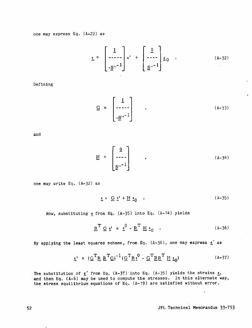
one mayexpress Eq. (A-22) as

E " c' +E_0 • (A-32)

Defining

G ..R

, (A-33)

and

H .. , (A-34)

one may write Eq. (A-32) as

: _G _' +H t0 • (A-35)

Now, substituting t from Eq. (A-35) into Eq. (A-14) yields

R T G t' : c° - R T H__O " (A-36)

By applying the least squares scheme, from Eq. (A-36), one may express _" as

c_' = (GTR RTG__)-I(GTRt 0 - GTRR T N c 0) (A-37)

The substitution of _" from Eq. (A-37)into Eq. (A-35) yields the strains _,

and then Eq. (A-6) may be used to compute the stresses. In this alternate way,

the stress equilibrium equations of Eq. (A-19) are satisfied without error.


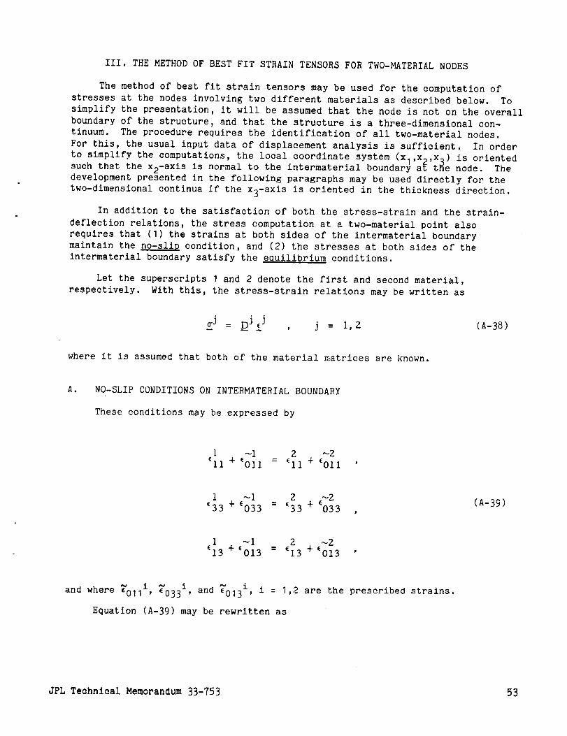
III. THEMETHODOFBESTFIT STRAINTENSORSFORTWO-MATERIALNODES

The methodof best fit strain tensors may be used for the computation ofstresses at the nodes involving two different materials as described below. Tosimplify the presentation, it will be assumedthat the node is not on the overallboundary of the structure, and that the structure is a three-dimensional con-tinuum. The procedure requires the identification of all two-material nodes.For this, the usual input data of displacement analysis is sufficient. In orderto simplify the computations, the local coordinate system (Xl,X2,X) is orientedsuch that the x2-axis is normal to the intermaterial boundary a_ t_e node. Thedevelopment presented in the following paragraphs may be used directly for thetwo-dimensional continua if the x3-axis is oriented in the thickness direction.

In addition to the satisfaction of both the stress-strain and the strain-deflection relations, the stress computation at a two-material point alsorequires that (I) the strains at both sides of the intermaterial boundarymaintain the no-slim condition, and (2) the stresses at both sides of theintermaterial boundary satisfy the equilibrium conditions.

Let the superscripts I and 2 denote the first and second material,

respectively. With this, the stress-strain relations may be written as

Z j = D j _J j = l 2 (A-38)Q J •

where it is assumed that both of the material matrices are known.

A. NO-SLIP CONDITIONS ON INTERMATERIAL BOUNDARY

These conditions may be expressed by

1 _I 2 ~2

_Ii + tOll = ell + EOII

1 _i 2 c_2 (A-39)c33 + c033 = _33 + 033 ,

1 ~i Z ~Z

_13 + c013 = _13 + _013

~ i _033 I, and _013and where _011 , i , i = 1,2 are the prescribed strains.

Equation (A-39) may be rewritten as


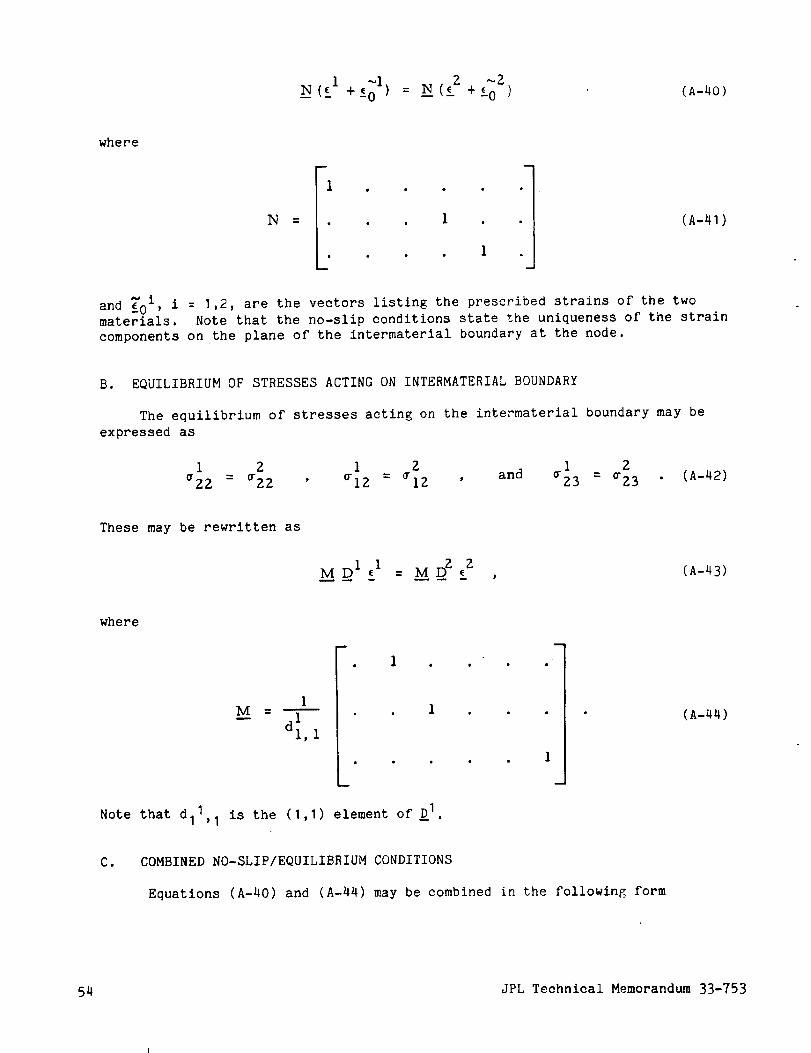
where

N ..

1

(A-41)

_0 i, i : 1,2, are the vectors listing the prescribed strains of the twoand

materials• Note that the no-slip conditions state the uniqueness of the strain

components on the plane of the intermaterial boundary at the node.

B. EQUILIBRIUM OF STRESSES ACTING ON INTERMATERIAL BOUNDARY

The equilibrium of stresses acting on the intermaterial boundary may be

expressed as

1 2 1 Z 1 2_22 = ¢22 ' _12 = ¢12 ' and _23 = _23 " (A-42)

These may be rewritten as

where

Note that d11,1

M B

m

1

1dl, 1

i

1

is the (1,1) element of _I

I

(A-44)

el COMBINED NO-SLIP/EQUILIBRIUM CONDITIONS

Equations (A-40) and (A-44) may be combined in the following form


C1 _i +b : Cz cz (A-45)

where

(A-46a)

and

= ~I -2 -i ~Z -I -2b T [0,0,0, ('011 -_011 )' ('033 -c033)' (_013-_013 )] (A-46b)

It can be shown that _J, j:I,2, are not singular, so long as _J, j:I,2, are

positive definite.

D. STRAIN-DEFLECTION RELATIONS

The intermaterial boundary divides the nodal line set of the node into two

partitions. The nodal lines of the intermaterial boundary may be included in

both partitions. Let mj, j=1,2, denote the number of nodal lines in the jth

partition. The strain-deflection relations of each partition may be written,

similar to Eq. (A-14), as

.T

R J cJ = !Oj , j=l, Z , (A-47)

where

R j : [r 1 ..... rmj]J , j=l,2 , (A-48)

.T

r3" : [pi i i i i i i i i i i i]j-t L IpI' PzPz ' PlPz ' P3P3 ' PlP3 ' Pz pSI , j:l,Z , (A-49)

and


E. COMPUTATIONOFSTRESSES

Since C_.2-1 exists, one may solve £2 from Eq. (A-45) as

2 C z'I 1 1 C 2-1: C _ + b (A-51)

Substituting _2 from Eq. (A-51) into Eqs. (A-47), yields

a

iTR_

R zT C z'I C 1

1E

r£O1 ]

I

i o2

where

(A-52a)

02 2 R 2T C Z-I_' = £0- b .

Equation (A-52a) may be solved for £I by least squares as

(A-52b)

cl (p,1R_.l T c1Tc z-T RZRZ T C z-1 -1 __ 1_ = + ..... c_.1) (1Rlc0

ITc 2-T - 2 02+C IR _ )(A-53)

Once the n_merical values of £I are computed, Eq. (A-51) is used to obtain

those of _. Then using Eq. (A-38), one can obtain the stresses.

IV. EXAMPLES

The following two examples illustrate the numerical results of the compu-

tational procedure developed in the previous section. The simple plane stress

element with linear displacement field and two degrees of freedom at each node

(Ref. 20) was employed.

The first example is that of a force acting at the end of a cantilevered

wedge as shown in Fig. A-I. The theory of elasticity solution is given in Ref.24 _ and is presented at section A-A by the curves labeled "a" in Figs. A-2 and

4The solution derived in Ref. 24 is for one material only and ignores the

clamped boundary conditions.


A,3 for the normal and shear stresses _22 and _12, respectively. Whenoneuses the finite element model of Fig. A-I, in which _he material in r_gionI is different from that in re_ion II (ET = 3.0 × 10 , E_T = 1.0 × I0°_I = _I = 0.3), the conventional best f_t strain methodZ_f Section II'givestwo sets of stresses, one at each side of the intermaterial boundary A-A.These are labeled "bi" and "bii" in Figs. A-2 and A-3, for material I andmaterial II. Clearly, the two sets of stresses at the intermaterial boundaryare not in equilibrium with each other.

Next, the application of the computational procedure developed in SectionIII with the same finite element model of Fig. A-I results in two sets of self-equilibrating stresses at the intermaterial boundary. These are coincident andare represented by the curves labeled "c" in Figs. A-2 and A-3. In addition tobeing in equilibrium, the stresses computed in this manner are more accuratethan either "bi" or "bii". It should be noted, however, that the degree of ac-curacy is stilI dependent upon other factors such as the finite element meshsize and the assumeddisplacement field within the elements; this is treatedfurther in the next example.

In the second example, the stresses produced by cooling an outside cylinderonto an inside one are computed. Initially, the outside radius of the innercylinder is equal to the inside radius of the outer cylinder (Fig. A-4). Thus,by uniformly cooling the outer cylinder by T = -200°F, the stress distributionin the two cylinders can be obtained by the elasticity theory and by theprocedures described. Becauseof the rotational symmetry, it is sufficient toconsider only a narrow wedgeof the cylinders as shown by the plane-stress fi-nite element model of Fig. A-5a.

Let MI and M2be the numberof equally spaced intervals in the innercylinder (material I) and outer cylinder (material I_, respectively. FigureA-5b shows the radial stress distribution --_I and _r obtained by the conven-

tional best fit strain method of Section A-II when MI = M2 = 5. The dis-

continuity in the radial stresses at the intermaterial boundary indicates the

degree of equilibrium violation.

In Table A-I, the intermaterial boundary stress values _r I, _r II, and

_t I, _t II in the radial and tangential directions are given. First, column

A gives the theoretical values, against which the finite element solutions

in B, C, and D of Table A-1 are compared by forming the percent error (in

parenthesis). Next, in group B, Table A-I, the intermaterial boundary stresses

of Fig. A-5b for MI = M2 = 5 are listed for the conventional best fit strain

method and followed by the values obtained when equilibrium is enforced accordingto Section III. The error associated with the conventional best fit strain

method with MI = M2 = 5 varies from +1.17 to +9.84% for _r I, _r II, and from

+0.7 to -3.3% for _t I, _t II. Although the generalized best fit strain method

of Section III did not greatly improve upon the errors in this case (+7.3

percent for _rI , _r II, and -7.1%, -1.3% for _t I, _tII), it has the advantageof producing a more consistent set of stresses which satisfy equilibrium,

compatibility and constitutive relations.

The results in group C and D of Table A-I show that the rate of con-

vergence of stresses as a result of varying the finite element mesh size is

almost the same for both computational procedures. Figure A-6, in which the


or.I, or.II are plotted for different finite element meshsizes,radial stressesemphasizes the sameconclusion.

V. CONCLUSIONS

Various schemesfor the stress computation in the finite element methodhave been suggested in which either equilibrium of forces or constitutive relationswere not necessarily satisfied. Amongthese schemesis the conventional bestfit strain method in which equilibrium is usually not satisfied at the inter-material boundaries. A generalization of this method was given in Section III,where full account is taken of all conditions of equilibrium, constitutive andcompatibility relations. The computation to accomplish this does not requireany additional data over that needed for the conventional best fit strain method.

Both methods proceed from the basic data necessary for the displacement method

of analysis.

From the presented examples it is shown that while the degree of equili-

brium violation in the conventional best fit strain method is dependent upon the

finite mesh size, overall better accuracy in satisfying equilibrium, constitutive

and compatibility relations is achieved in the stresses computed by the generalized

best fit strains developed in Section III. Similar improvements can be expected

from an analogous generalization of other schemes for the stress computation.


o_._

{0

{0

GO

_,_

e_

0

or-I

T.,

0

0

L

0

_J

a)

,PI

J=

c.

"0

I

0

o

ic

&-

Jl

7-

01

tl

G

N

.¢1

m m__ _.H

OC *,J ..-I

Ip

N_

.-_ 0

0,_

0

go$

m mH

o._._

o

$

e'.l_

ao

o o

I

'-r

g,

÷

k_

÷

i I I +

8 _ _ 3

R

_ en

,., "2 g

_, _ ; .

e %- b"


E

I )A

Fig. A-I. Plane stress finite element

model of a force acting at the end

of a wedge

//

/

o///

c/

"a", THEORETICAL (REF. 24)

"hi" and "bll" t CONVENTIONAL

BEST FIT STRAIN, SEC. II

"c" • GENERATED BEST FITSTRAINS,. SEC. III

Fig. A-2. Normal stresses o'22 at A-A


q_

"a", THEORETICAL (REF. 24

012

Q

/'/b I

///,c

"hi", "bll" t CONVENTION_ L BEST FIT STRAINSt SEC. II

"c", GENERALIZED BESTFIT STRAINS, SEC. III

Fig. A-3. Shear stresses _12 at A-A

//

/

\

O UTSIDE CYL INDER

E " 103.423 GN/m 2

(15 x 106 Ib/ino 2)

- 0.3

e I 12 x 10.6 crn/cm/_C

( 6,67 x 10-6 in./in./°F)

INSIDE CYLINDER

E = 206.846 GN/m 2

F_** (0._; 106 Ib/in'2)

5.0_ ¢m (2 in°)

qll_86 15.24 cm_--_(6 in.)

• On1

(9 in.)

Fig. A-4. Two-cylinder shrink fit


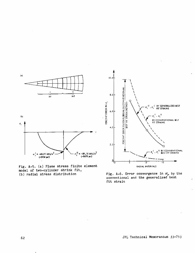
(a)

Mt A_2

(b)

a r

o"t = -40.91 MN/m2f

(_934 psi)

_39.15 MN/m 2

(-5678 Psi)

Fig. A-5. (a) Plane stress finite element

model of two-cylinder shrink fit,

(b) radial stress distribution

Lt)

z

6.0u_

4.0

2.0

- --\\

-7

c \

\ a II I BY GENERALIZEDBEST

Z _S r ,Or FITSTRAINS

_ _ 1_ BY CONVENTIONAL BEST

z_

-- _ , Orll BY CONVENTIONAL

-- _ _ °rl BEST FIT STRAINS

5 1o 15

RADIAL INTERVALS

Fig. A-6. Error convergence in _r by the

conventional and the generalized best

fit strain


APPENDIX B

COMPOSITION OF THE SUBSTRATE MATERIALS

(1)

(2)

(3)

(4)

(5)

The five substrate materlals tested in this program are:

Kapton-H: a polyimide film made by E. I. DuPont DeNemours and Co.(Type

30OH, from Mill Roll 04493). It was obtained with a thickness of 0.00762 cm

(0.003 in.) in a roll 30.48 cm (12 in.) wide.

Kapton-F: a laminated film made by DuPont, consisting of a 0.00508-cm

(O.O02-in.) layer of Kapton-H sandwiched between 2 layers, each 0.00127 cm

(0.0005 in.) thick, of Teflon (Type 300F 929, from Mill Roll 00809).

It was obtained with a total thickness of 0.00762 cm (0.003 in.) in

a roll 30.48 cm (12 in.) wide.

Teflon: a fluorinated ethylene propylene film made by DuPont (Type FEP

500A). The material was obtained with a thickness of 0.0127 cm (0.005 in.)

in a roll 60.96 cm (24 in.) wide. It was not possible to determine

the mill roll from which it was cut.

Tedlar: a polyvinyl fluoride film made by DuPont (Type 200 SG 40 TR,

from Sllt Roll 7E014140). It was obtained with a thickness of 0.0050_

cm (0.002 in.) in a roll 30.

PG-402 0/0: a fiberglass-reinforced polyimlde made by the Mica Corp-

oration, Culver City, Cal. (from Lot 11974-2028-I). The symbol 0/0

refers to no copper cladding. It was obtained in 91.44 x 45.72 cm

(36 x 18 in.) sheets with a thickness of 0.00635 cm (0.0025 in.).

The 1080 plain weave fiberglass cloth had a warp of 60.and a fill of

47; an amino silane finish was put on the cloth for better wetting

during the fabrication of the PG-402.


APPENDIXC

COEFFICIENT OF THERMAL EXPANSION FOR SUBSTRATE MATERIALS:

TEST PROCEDURE AND INSTRUMENTATION

The linear expansion coefficients were computed from measurements of the

specimen length variation with temperature. A brief description of the methods

and instruments follows. The test apparatus was a quartz tube dilatometer

(Figs. C-I and C-2) built in accordance with methods explained in ASTM E-228.

The test specimens were held in tension by Invar grips attached to concentric

fused silica tubes. Changes in the relative positions of the upper ends of the

tubes (representing changes in length) were recorded with a 0.000254 cm (0.0001

in.) dial indicator.

The lower end of the tube was temperature-stab_iize_ between -195.6 and

204.4°C (-320 and 400°F). The chamber was then sealed and a dry helium purge

was maintained inside the tubes. The chamber temperature was stabilized

electrically and monitored by three thermocouples. The effects of dimensional

changes in the low expansion Invar grips were further minimized by the self-

compensating design.

The test specimens were approximately 9.398 cm (3.7 in.) long with a maxi-

mum width of 2.286 cm (0.9 in.) and a maximum thickr_ess of 0.2286 cm (0.090

in.).

The test procedure was to adjust the chamber temperature until the specimen

temperature was constant. Accuracy of the measurement was approximately ±5 ×10-_ cm/cm over the full temperature range.


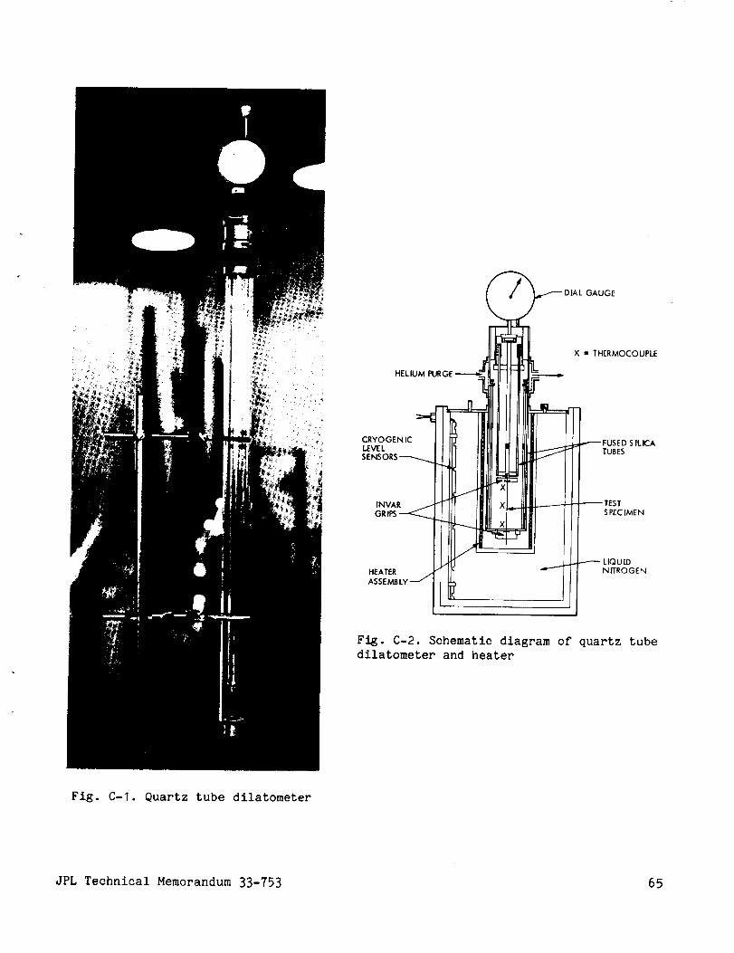
UGE

HELIUM PURGE

X = THERMOCOUPLE

CRYOGEN ICLEVELSENS_

TUBESILICA

INVARSPEC IME N

LIQUIDHEATER NITROGEN

Fig. C-2. Schematic diagram of quartz tubedilatometer and heater

Fig. C-I. Quartz tube dilatometer


APPENDIX D

TEST SETUP AND SPECIAL TECHNIQUES

USED IN MECHANICAL PROPERTY MEASUREMENTS

I. TEST SETUP

The mechanical tests were performed on an Instron tensile testing mach-

ine. Figures D-I and D-2 show photographs of the machine, with a typical

polymer sample in the grips of the clamping device in the test chamber.

Liquid nitrogen was used as the coolant for low-temperature measurements,

in preference to carbon dioxide, which was found to produce anomalous surface

effects on the samples.

Special grips were designed and made out of aluminum for applying a

tensile load to the test specimens (see Fig. D-I). About two to three inches

(depending upon material thickness) of material was wrapped around a 1.27-cm

(0.5-in.) diameter spool which was inserted in a clamping device. To increase

the coefficient of friction, the spool surface was sandblasted. The clamps

were locked in place by a thumb screw in the bottom grip and by an Allen cap

screw in the top grip. The test specimen was in the line of applied force

between the cross head and the load cell in the top of the Instron tensile

machine.

Each clamping device was fastened to a ball socket joint which provided an

effective universal joint immediately adjacent to the specimen grips. From

studies of the precision mechanical properties of materials, it was shown that

this method of specimen alignment minimizes any bending in the test specimen. A

minimum load was always maintained to preserve the axiality of the specimen.

II. PHOTOGRAPHIC METHOD FOR STRAIN MEASUREMENT

Because the test specimens were very thin polymer films, Poisson's ratio

measurements using conventional strain gauges resulted in considerable errors.

The errors arise from the fact that the gauge stiffness is comparable to the

specimen stiffness. Thus, to obtain more accurate strain measurements, a

special photographic method was developed. First, a reference pattern of

fiducial crosses was inked on the surfaces of each test specimen, as shown in

Fig. D-3. The total array of the crosses, on 0.254-cm (0.l-in.) centers,

occupied an area 2.54 by 10.16 cm (I by 4 in.) long. Several methods of

applying the patterns were evaluated before a silk screen method was selected.

When the test specimen is loaded in the testing machine, these fiduclal

patterns deform laterally and longitudinally. The relative lateral to longi-

tudinal deformation of a central portion away from the edges of each specimen

provided a measure of Poisson's ratio. The deformed patterns were photographed

for purposes of later measurements. A tripod-mounted 35-mm Pentax camera

fitted with a 100-mm f/4 bellow Takuman lens and a shutter speed of I/8 sec was

used for this purpose.


All tests, except those at 25°C, were made inside an environmental chamber.PhotOgraphsfrom 38.1 cm (15 in.) were taken through a double glass window(specimen to camera). Figure D-4 showsa typical distortion of the fiducial

patterns for Kapton-H for conditions of zero, 14, and 32% strains at I00°C.

The distorsion is much more pronounced in the case of the Teflon, Fig. D-5. In

the latter, appreciable distortion occurs up to 125% strain without specimenbreakage.


_,ALL-SOCKET JOINT

LOCKING SCREW

SPOOL

CLAMPING DEVICE

THERMOCOU PLE

BALL_OCK_ JOINT

Fig. D-I. Tensile testing machine:

2.54-cm (l-in.) gauge length specimen

mounted in grips

I

Fig. D-2. Tensile testing machine:

2.54-cm (l-in.) gauge length specimen

mounted in testing chamber


DIMENSIONS IN CENTIMETERS AND INCHES

EDGE OFSPECIMEN

0.102(0.040)TYP

0,254 0,127 .._"----- (o.loo) _= (0.050)

0°203

(0.08_) TYP0.2O3 --I

0.254 (o.100) TYP .,,---(O.OSO) TYP'--*'I

o O¢TYP

-----1

0.0254(o,o10) R MAXTYP

Fig. D-3. Dimensions of "plus signs" used

as fiducial pattern

oF Poor QUALn_


++++÷_4÷++_

+÷÷_+÷_+_÷_

+++_+44--4- 4- 4-÷:4

{a) NO STRAIN

_-+÷__,._-, _ -.

(b) 14% STRAIN

?o JPL Technical Memorandum 33-753

• . .÷ __+++, ...........

........... 22#2#TI2ZI--._#° .+.

(a) NO STRAIN (b) 43% STRAIN

(c) 65% STRAIN

r(d) 89% STRAIN

(e) 9_/oSTRAIN (0 125% STRAIN

Fig. D-5. Distortion of the baseline fiducialpatterns for Teflon, 2.54 em (l-in.) gauge

length, -I00°C

_P_GI_A_ PAG]_ IS

OF POOR QUALIT_


APPENDIXE

PROCEDUREFORSPECIMENPREPARATIONFORMECHANICALPROPERTYTESTS

Test specimens 30.48 cm (12 in.) long by 2.54 cm (I in.) wide were cutusing a double-bladed tool developed for this program. The cutting apparatus(Fig. E-I) consists of a double-grooved base plate, a clamping bar, and a blockfor mounting two razor blades. Figure E-2 shows the apparatus assembledpreparatory to cutting a Kapton-H specimen.

A strip of material several inches wide is placed upon the base plate.The clamping bar is then placed over it, positioned by two locating pins at theends. Theblock holding the razor blades is then drawn along the clamping barwith a slow, steady motion. In order to avoid splits or tears at the edges ofthe specimens, the razor blades were changed frequently. Cut edges wereexaminedwith an electron microscope, but the shallow depth of focus preventedsatisfactory analysis. Randomspecimens were examined in the scanning electronmicroscope, after application of a thin coating of carbon to render the surfaceselectrically conductive. Typical edge effects are shownin Figs. E-3 throughE-7. Tedlar (Fig. E-3) had the "cleanest" cut because it had the smoothest cutface and no burr at the bottom where the blade left the material. Teflon edges(Fig. E-4) were marked by a pronounced burr at the bottom surface and a slightlyrough cut face. Figure E-5 (Kapton-H) showeda slightly serrated cut edge withonly a very small burr. Kapton-F (Fig. E-6) also showeda burr at the bottomsurface of the outer layer of Teflon. None of the unreinforced polymer specimensshowededgedefects that could be considered as sources of premature failure.The cut edge of PG-402(Fig. E-7) was very rough becauseof the fiberglasscontent.

72 JPL Technical Memorandum33-753

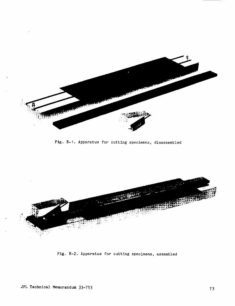
Fig. E-I. Apparatus for cutting specimens, disassembled

Fig. E-2. Apparatus for cutting specimens, assembled


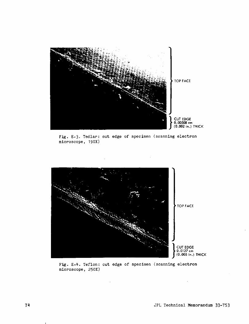
TOP FACE

Fig. E-3. Tedlar: cut edge of specimen

microscope, 190X)

! CUT EDGE• 0.00508 cmm (0.002 in.) THICK

!

scanning electron

!

I

TOP FACE

i

CUT EDGE• 0.0127 cm

(0.00.5 in.) THICK

Fig. E-4. Teflon: cut edge of specimen (scanning electron

microscope, 250X)


TOP FACE

CUT EDGE0.00762 cm(0.003 in.) THICK

Fig, .E-5. Kapton-H: cut edge of specimen (scanning electron

microscope, 225X)

TOP FACE

t CUT EDGE0.00762 cm(0.003 _n.) THICK

BURR

Fig. E-6. Kapton-F: cut edge of specimen (scanning electron

microscope, 210X)


TOP FACE

CUT EDGE0.00635 ¢m(0.0025 in.) THICK

Fig. E-7. PG-402: cut edge of specimen (scanning electron

microscope, 100X)

76JPL Technical Memorandum 33-753

REFERENCES

I •

•

•

1

•

1

.

o

.

10.

11.

12.

13.

Salama, M. A., Rowe, W. M., and Yasui, R. K., "Stress Analysis and Design

of Silicon Solar Cell Arrays and Related Material Properties," in Conference

Record of the Ninth IEEE Photovoltaic Specialists Conference, pp. 146-

157, Silver Spring, Md, May 1972.

Salama, M. A., Rowe, W. M., and Yasui, R. K., Thermoelastic Analysis of

Solar Cell Arrays and Their Material Properties, Technical Memorandum

33-626, Jet Propulsion Laboratory, Pasadena, Calif., Sep. 1973.

Hartzman, M., "Stress-Strain Relations for Materials with Different

Tension, Compression Yield Strengths," J. AIAA, Vol. II, No. 3, PP.

378-379, Mar. 1973.

Utku, S., and Akyuz, F. A., ELAS - A General-Purpose Computer Program

for the Equilibrium Problems of Linear Structures: User's Manual, Tech-

Report 32-1240, Vol. I, Jet Propulsion Laboratory, Pasadena, Calif.,

Feb. 1968.

Gupta, K. K., Akyuz, F. A., and Heer, E., VISCEL - A General-Purpose

Computer Program for Analysis of Linear Viscoelastic Structures: User's

Manual, Technical Memorandum 33-466, Vol. I, Rev. I, Jet Propulsion

Laboratory, Pasadena, Calif., Oct. 1972.

"Mechanical Design Data for Teflon Fluorocarbon Resins," Plastic Depart-

ment, DuPont Company, Wilmington, Del.

Clark, F. M., Insulating Materials for Design and Engineering Practice,

John Wiley, New York, p. 603, 1962.

Nielsen, L. E., Mechanical Properties of PglFmers, Van Nostrand Reinhold

Co., 1962.

Clark, E. S., "Morphology and Physical Properties of Crystalline Polymers,"

Polymer Preprints, Vol. 14, No. I, pp. 88-91, May 1973.

Parrish, M., and Brown, N., "Environmental Effects on the Tensile Deforma-

tion of Polymers at Low Temperatures," J. Macromal Sci-Phys., B8 (3-4),

p. 655, 1973.

Olf, H. G., and Peterlin, A., "Crazing in a Crystalline Polymer (Is•tactic

Polypropylene) and the Role of N202 and CO 2 as Crazing Agents," polymer,Vol. 14, pp. 78-79, Feb. 1973.

Zienkiewicz, O. C., The Finite Element Method in Engineering Science

McGraw-Hill, New York, 1971.

Wilson, E. L., "Finite Element Analysis of Two-Dimensional Structures,"

Ph.D. Thesis, University of California, Berkeley, 1963.


14.

15.

16.

17.

18.

19.

20.

21.

22.

23.

Utku, S., "Best Fit Stress Computation in Displacement Methods," paper

presented in the Discrete and Continuum Concepts in Micro and Macro

Mechanics, EMD Specialty Conference, ASCE, North Carolina State University,

Raleigh, N. C., Nov. 1967.

24.

Oden, J. T., and Brauchli, H. J., "On the Calculation of Consistent Stress

Distribution in Finite Element Applications," Int. J. Numer. Meth. Eng.,

Vol. 3, PP. 317-325, 1971.

Stein, E., and Ahmad, R., "On the Stress Computation in Finite Element

Models Based Upon Displacement Approximations," Comp. Meth. Appl. Mech.

Eng., Vol. 4, pp. 81-96, 1974.

Stricklin, J. A., "Computation of Stress Resultants From the Element

Stiffness Matrices," J. AIAA, Vol. 4, pp. 1095-1096, 1966.

Navaratna, D. R., "Computation of Stress Resultants in Finite Element

Analysis," J. AIAA, Vol. 4, pp. 2058-2060, 1966.

Argyris, J. H., and William, K. J., "Some Considerations for the Evalua-

tion of Finite Element Models," 2rid International Conference on Structural

Mechanics and Reactor Technology, Berlin, 1973.

Utku, S., ELAS - A General-Purpose Computer Program for the Equilibrium

Problems of Lin@ar Structures, Vol. II, Documentation of the Program ,

Technical Report 32-1240, Jet Propulsion Laboratory, Pasadena, Calif.,

Sept. 1969.

Utku, S., Rao, M. S. M., and Dvorak, G., ELAS65 Program for Elastic-Thermo-

Plastic Solids and Structures, Structural Mechanics Series No. 15, School

of Engineering, Duke University, Durham, N. C., 1973.

Utku, S., Tarn, J., and Dvorak, G., ELAS_ Program for Thermo-Visco

Elashic-Plastic Solids and Structures, Structural Mechanics Series No.

21, School of Engineering, Duke University, Durham, N. C., 1974.

Nay, R. A., and Utku, S., "An Alternative for the Finite Element Method,"

Variationa ! Methods in Engineering, Vol. II, Department of Civil Engineer-

ing, Southampton University Press, pp. 3/62-3/74, 1973.

Timoshenko, S., Strength of Materials, Part II, 3rd ed., D. Van Nostrand,

1956.

78 JPL Technical Memorandum 33-753NA_-JPL-.ComI., L.A., _lif

technical memorandum 33-753 - nasa · technical memorandum 33-753 ... (jet propulsion lab.) 87 p hc...

Documents