technical note: a new method for the lagrangian tracking

Atmos. Chem. Phys., 9, 2577–2595, 2009www.atmos-chem-phys.net/9/2577/2009/© Author(s) 2009. This work is distributed underthe Creative Commons Attribution 3.0 License.

AtmosphericChemistry

and Physics

Technical note: a new method for the Lagrangian tracking ofpollution plumes from source to receptor using gridded modeloutput

R. C. Owen1,2 and R. E. Honrath1,2,3

1Department of Geological and Mining Engineering and Sciences, Michigan Technological University, USA2Department of Civil and Environmental Engineering, Michigan Technological University, Houghton, Michigan, USA3Atmospheric Sciences Program, Michigan Technological University, USA

Received: 23 July 2008 – Published in Atmos. Chem. Phys. Discuss.: 3 November 2008Revised: 9 March 2009 – Accepted: 9 March 2009 – Published: 8 April 2009

Abstract. Lagrangian particle dispersion models (LPDMs)are powerful and popular tools used for the analysis of atmo-spheric trace gas measurements. However, it can be difficultto determine the transport pathway of emissions from theirsource to a receptor using the standard gridded model out-put, particularly during complex meteorological scenarios.In this paper we present a method to clearly and easily iden-tify the pathway taken by only those emissions that arriveat a receptor at a particular time, by combining the standardgridded output from forward (e.g., concentration) and back-ward (e.g., residence time) LPDM simulations. By compar-ing the pathway determined from this method with particletrajectories from both the forward and backward models, weshow that this method successfully restores much of the La-grangian information that is lost when the data are gridded. Asample analysis is presented, demonstrating that the source-to-receptor pathway determined from this method is more ac-curate and easier to use than existing methods using standardLPDM products (gridded fields of, e.g., concentrations andresidence time). As demonstrated in an evaluation and an ex-ample application, the method requires agreement betweenthe transport described by the forward and backward simula-tions and thus provides a means to assess the quality and re-versibility of the simulation. Finally, we discuss the potentialfor combining the backward LPDM simulation with griddeddata from other sources (e.g., chemical transport models) toobtain a Lagrangian sampling of the air that will eventuallyarrive at a receptor. Based on the advantages presented here,this new method can complement or even replace many ofthe standard uses of backward LPDM simulations.

Correspondence to:R. E. Honrath([email protected])

1 Introduction

The transport experienced by a plume of emissions can havea significant influence on its chemical composition. Dry de-position, which is an important removal mechanism for manytrace gases, occurs in the boundary layer (BL). Significantwet deposition is often associated with strong uplift from theBL into the free troposphere (FT) (e.g.,Stohl et al., 2002b).For example, soluble species, such as HNO3, can be removedduring this uplift. Once in the FT, however, the chemicalcomposition of an air mass is more dependent on photochem-istry and mixing (e.g.,Methven et al., 2003). Thus, knowingthe amount of time an air mass spends in the BL, the timingand location of uplift, the time spent in the FT, and the rel-ative amounts of mixing during these processes is essentialto a complete understanding of the chemical transformationsoccurring in an air mass. As a result, determining these trans-port characteristics for a plume of emissions as it travels fromits source to a downwind sample location has been an impor-tant part of many measurement efforts (e.g.,Rex et al., 1998;Stohl and Trickl, 1999; Trickl et al., 2003).

The atmospheric transport pathway through which emis-sions traveled to a downwind receptor is often deduced withLagrangian models, either trajectories or Lagrangian parti-cle dispersion models (LPDMs). Trajectories remain pop-ular because they are easy to use, but they are limited bytheir inability to describe the deformation of an air mass andthe concentration gradients of chemical trace substances inthe atmosphere (Stohl et al., 2002a; Methven et al., 2006).LPDMs are superior because they address both these issues(e.g., Han et al., 2005), but they also have shortcomings.Their output is more complex than that of trajectory modelsand much of the Lagrangian information is lost in the process

Published by Copernicus Publications on behalf of the European Geosciences Union.

http://creativecommons.org/licenses/by/3.0/

2578 R. C. Owen and R. E. Honrath: Lagrangian plume tracking

of calculating concentrations on a Eulerian-type output grid.While some work has been done to simplify the LPDM out-put (e.g.,Stohl et al., 2002a), there remains a need for newproducts to succinctly describe LPDM output. Additionally,there are no methods available to retrieve the Lagrangian in-formation that is lost when the output is gridded, short ofsaving particle trajectories. While particle trajectories pro-vide useful information, they are typically not saved duringLPDM simulations because they increase the time it takes torun and process a simulation and require large amounts ofstorage and memory. Particle trajectories also add a level ofcomplexity in interpreting the output and are generally usedonly in advanced LPDM studies (e.g.,Stohl et al., 2004).

Traditionally, studies that use LPDMs to perform a de-tailed analysis of the transport of emissions to a particularreceptor use both forward simulations (simulations of atmo-spheric concentrations resulting from an emissions field) andbackward simulations (simulations of the upwind transportof air ultimately reaching a receptor), but present them as in-dividual products. For example,Stohl et al.(2003) used for-ward simulations to understand the large scale transport fromNorth America to aircraft-based sample locations over theNorth Atlantic and Europe, while backward simulations wereused to determine the age distribution of the trace substancein the receptor cells, to determine the specific source regionscontributing to the trace substance enhancements in the re-ceptor cells, and to determine the transport pathway to thereceptor. They assumed that the backward plume matchedthe pathway taken by emissions, which was reasonable onlybecause this particular transport experienced very little defor-mation. Owen et al.(2006) analyzed the forward and back-ward products together, by presenting snapshots of the twosimulations side-by-side, but detailed analysis of transportwas limited to only those backward simulations that expe-rienced little deformation between the source and receptor.Despite these applications, there remains a disjunction be-tween the information provided by forward and backwardLPDM simulations.

In this paper, we present and evaluate a new method, theproduct of which we call a folded retroplume. The foldedretroplume addresses two of the shortcomings of the LPDMby simplifying the LPDM output and allowing the retrieval ofsome of the Lagrangian information that is lost in the processof calculating gridded (Eulerian) output fields. The purposeof the folded retroplume is to provide a way to efficiently andaccurately determine the transport pathway of emissions to areceptor, highlighting only those emissions that arrive in thereceptor cell at the time of interest, using standard griddedoutput fields from an LPDM. As we show below, this canbe accomplished by convolving the standard output from aforward model simulation with that from a backward modelsimulation, bringing the information from the forward andbackward models together in such a way that even complextransport scenarios can be analyzed. When used in this way,the forward model describes the amount of a trace substance

in the atmosphere, while the backward model describes howmuch of this trace substance will arrive in the receptor cellat a given time. The folded retroplume is easier to use andmore accurate than using standard gridded LPDM productsalone. Additionally, the method is superior to similar meth-ods available with trajectories, as it retains the advantages ofLPDMs, e.g., the ability to describe dispersion and to pur-vey information about the relative concentration of the tracesubstance along the transport pathway. Since the method re-quires an agreement in the transport described by the twomodel simulations, it also allows for an assessment of thequality and reversibility of the simulation. We also introducesimilar uses of the backward model with alternate Eulerianfields that describe the state of the atmosphere (e.g., outputfrom a chemical transport model) to determine physical andchemical properties of an air mass as it travels toward a re-ceptor.

Below, we provide a method overview (Sect.2), evalua-tion (Sect.3), and example (Sect.4) that are based on theLPDM FLEXPART (Stohl et al., 2005), one of the more pop-ular LPDMs in use today. Although the presentation is some-what specific to this model, the method should be valid forany LPDM with an appropriately employed backward mode,because all LPDMs have the property that they are essen-tially self-adjoint, i.e., the backward mode only requires thereversal of the direction of advection to give the transportsensitivity for a receptor cell (Seibert and Frank, 2004).

2 Method overview

We begin with a brief outline of the formulation of the modeloutput and the folded retroplume, followed by a simple casethat illustrates the folded retroplume. We rely heavily on themodel theory presented byStohl et al.(2005) andSeibert andFrank(2004) and refer the reader to these sources for moredetailed reviews of LPDM theory and technical descriptionsof LPDM operational details. We also recommendFleschet al.(1995) andLin et al. (2003) for additional informationon backward LPDM modeling andErrico (1997) and for ad-ditional background on general adjoint model theory.

2.1 Formulation of the model output and folded retro-plume

In this section, we review the calculation of the griddedmodel output, starting with the forward mode, and provideseveral formulations involving the folded retroplume. Thecalculations presented in this section are limited to instan-taneous model output. (The use of averaged model outputcan complicate the interpretation of folded retroplumes andis thus discussed in Sect.3.3.)

Atmos. Chem. Phys., 9, 2577–2595, 2009 www.atmos-chem-phys.net/9/2577/2009/

R. C. Owen and R. E. Honrath: Lagrangian plume tracking 2579

2.1.1 Standard output from the forward mode

In the forward mode, particles are released at the source andthen transported forward in time, according to the mean andturbulent wind components (Stohl et al., 2005). The mass ofeach particle at the time of emission is based on the strengthof the source. Concentrations are calculated by summing themass of all the particles that reside in each grid cell. We firstconsider only a puff of emissions and focus on one downwindgrid cell (j ) at a single model time (t). The instantaneousgridded concentration (c) from a puff of emissions releasedat timet0 is thus:

cj, t=1

Vj

∑Vj

mj, t0·pj, t ·fj , (1)

whereVj is the volume of the cell and the summation is overall particles that reside inVj at time t . mj,t0 is the initialmass of the particle,fj is the sampling kernel, which canbe used to distribute the mass of the particle across multiplegrid cells, andpj,t is the transmission function, which de-scribes the percentage of the particle mass remaining fromremoval processes (seeStohl et al., 2005 and Seibert andFrank, 2004for a more complete description of these terms).In order to calculate the mass mixing ratio, the concentrationis first divided by the local air density (from the meteorolog-ical data). The volume term from the concentration cancelswith the volume term from the local air density, leaving themass of air in the cell (mj,air) and the summation of the massof the particles in the cell. The volume mixing ratio (χ ) isobtained by multiplying this value by the ratio of the meanmolecular mass of air (Mair), to that of the trace substancebeing modeled (Mtr ), giving the volume mixing ratio:

χj,t=

(Mair

Mtr

) (1

mj, air

) ∑Vj

mj, t0·pj ·fj . (2)

Mixing ratios are saved at each time for each grid cell in themodel domain, giving a 3-dimensional matrix (χt) of the vol-ume mixing ratios for allj (i.e., eachx, y, andz component).

2.1.2 Standard output from the backward mode

In the backward mode, particles are initiated in a single re-ceptor volume (j ′) over a short interval (t ′, the arrival time)and transported backward in time by reversing the directionof the mean wind. The mass of each particle is normalizedby the total mass released in the receptor (mtot), giving eachparticle units of mixing ratio, such that each particle repre-sents one part of the air in the receptor at the release (i.e.,arrival) time and the distribution of the particles indicates thelocation of the receptor air at each upwind time. The back-ward output is gridded by summing these mixing ratios ineach cell, giving the sensitivity (S) of the receptor to the masspresent in the upwind cell:

Sj, t, (j ′,t ′)=

∑Vj

mj, t ′

mtot·pj, t ·fj , (3)

Again, the output is saved at each time for each grid cell,giving a 3-dimensional matrix (St, (j ′,t′)) of the sensitivity forall j . The output of the backward mode is referred to as thesensitivity plume, or the retroplume.

2.1.3 The folded retroplume – combining model out-put to determine the source-to-receptor transportpathway

The folded retroplume at timet is the Hadamard (or entry-wise) product of the mixing ratio matrix (χt) from the for-ward mode and the sensitivity matrix (St,(j ′,t′)) from thebackward mode. In terms of an individual cell, the mixing ra-tio (Eq.2) indicates the amount of emitted trace substance inthe given cell, and the sensitivity (Eq.3) indicates the amountof air in the cell that will be transported to the receptor. Bymultiplying the two values, we can determine the amount ofthe trace substance in the cell that will eventually arrive atthe receptor (j ′) at the arrival time (t ′). Note the units forthis operation. We begin with the volume mixing ratio, withunits of parts of trace substance per parts of air in the cell.This is multiplied by the sensitivity, with the units of parts ofair in the cell per parts of air in the receptor. The resultingproduct calculated for a specific cellj has units of volumemixing ratio, and indicates the portion of the mixing ratio inthe receptor att ′ (the sensitivity plume arrival time) resultingfrom the transport of trace substance through cellj at timet .That is, the units are parts of trace substance in the cell perpart of air at the receptor. As this mixing ratio results fromonly a part of the sensitivity field (the individual upwind cellconsidered here), we call the product the partial mixing ratio(PMR):

PMRj, t, (j ′, t ′)=Sj, t, (j ′, t ′)·χj, t , (4)

wheret is the model time. The PMR will clearly be smallor zero when there is either little of the trace substance in acell or small sensitivity. Conversely, if there is a significantamount of trace substance in a cell and a large sensitivity,then the PMR will also be large, indicating the location oftrace substance that travels from the source to the receptor.The 3-dimensional matrixPMRt,(j ′,t′) indicates the distribu-tion at timet of the trace substance that will ultimately arriveat the receptor at timet ′, while the matrixPMR(j ′,t′) at multi-ple times shows the transport pathway of the trace substancebetween the source and receptor.

Up to this point, we have only considered a puff of emis-sions in the forward model, which is not the typical modelsituation. Normally, emissions are continuously released intothe forward simulation and each particle is carried in themodel for a set number of days and then dropped. Thus,the mixing ratio from the forward model (χj,t ) consists ofparticles released over a range of times and can be dividedinto age classes, according to the length of time the particleshave been in the model (the age of the particles). If the age ofthe trace substance is not taken into account when computing

www.atmos-chem-phys.net/9/2577/2009/ Atmos. Chem. Phys., 9, 2577–2595, 2009


the PMR then the folded retroplume calculation will includeparticles that would be dropped from the forward simulationbefore they would be transported to the receptor. To avoidthis, the age of forward model trace substance in Eq. (4)(χj,t ) must be less than the time difference between the re-lease time in the backward model (that is, the arrival time)and the sample time (t). If we have a forward simulation thatcarries particles forAf days and a backward simulation withan arrival time oft ′, then the PMR at some intermediate time(t) should be:

PMRj, t, (j ′, t ′)=Sj, t, (j ′, t ′)·

Af −(t ′−t)∑i=0

χj, t, i . (5)

wherei indicates the available age classes in days from theforward model.

The PMRs at any upwind time may be summed over themodel domain to determine the mixing ratio from all (ap-propriately aged) emissions that are present in the model atthat time. If no more emissions are added to the atmospherebetween that time and arrival time, then this sum would beequal to the mixing ratio in the receptor (j ′) at the arrivaltime (t ′). Thus, we call this sum the upwind mixing ratio(UMR):

UMRt, (j ′, t ′)=

∑j

PMRj, t, (j ′, t ′). (6)

The UMR is equivalent to a sensitivity-weighted average ofthe upwind mixing ratio field and can increase or decrease,depending on the relative rates of emission and removal pro-cesses. For example, if emissions are added to the atmo-sphere between time steps and no removal processes are con-sidered, the change in the UMR from timet to t+1 shouldbe

UMRt+1, (j ′, t ′)=UMRt, (j ′, t ′)+

∑j

Sj, t, (j ′, t ′)·Ej, t , (7)

whereEj,t are the emissions released into the model at timet and

∑j Sj,t,(j ′,t ′)·Ej,t is the so called source contribution

(Stohl et al., 2003). However, if no removal processes areconsidered and if no emissions are added to the atmosphereafter timet (or if no emissions are added in areas with sensi-tivity – the region where the plume is located), then the UMRshould remain constant.

The UMRs therefore provide a means to evaluate the evo-lution of the mixing ratio of the receptor air during trans-port. For instance, the timing and location of wet removalcould be determined by comparing the UMRs from twofolded retroplumes, one computed from forward and back-ward simulations with no wet removal and one computedfrom forward and backward simulations that include wet re-moval. Section5 will discuss other potential applicationsusing the UMRs derived from folding a backward simulationwith mixing ratio fields from alternate sources.

2.2 Illustrative case

Here we present the application of our method to a simplecase in order to illustrate the folded retroplume. The case isbased on a puff of CO emissions released into the forwardmodel from the Boston area, into the box bounded by 41–43◦ N latitude and 73–75◦ W longitude, from the surface upto a height of 250 m a.s.l. Emissions were released over a 1-hperiod, from 15:00–16:00 UTC on 14 May 2005 and werebased on the EDGAR Fast Track 1999 inventory (Olivieret al., 1996). The backward simulation was initiated at thePico Mountain observatory, located on the Azores Islands inthe Central North Atlantic Ocean, into the box bounded by38.5–39.0◦ N latitude 28.5–28.0◦ W longitude, from an alti-tude of 2000–2250 m a.s.l. Particles for the backward sim-ulation were also released over a 1-h period from 00:30–01:30 UTC on 19 May 2005.

FLEXPART version 6.2 was used, driven with data fromthe European Centre for Medium Range Weather Forecasts(ECMWF) (ECMWF, 2005) with 1◦

×1◦ horizontal reso-lution, 60 vertical levels and a temporal resolution of 3 h,using meteorological analyses at 00:00, 06:00, 12:00 and18:00 UTC and ECMWF 3-h forecasts at intermediate times(03:00, 09:00, 15:00 and 21:00 UTC). The output was savedwith a grid size of 0.5◦×0.5◦ in the horizontal and 250 m inthe vertical, from 0–7000 m a.s.l. The sampling kernel wasturned off and instantaneous fields were saved (see Sect.3.3for a description of these model settings and more detailson their impact on the folded retroplume). 500 000 parti-cles were used for the forward simulation and 2000 particleswere used for the backward simulation, resulting in a total of670 forward particles and 634 backward particles that suc-cessfully travel between the source and receptor cells.

Figure1a and b shows the plan view and longitude-heightcross section of the CO plume 1.5 days after the forward-model puff release. Figure1c and d shows plan view andlongitude-height cross section of the sensitivity plume 3 daysupwind of the release at the receptor (and at the same time asshown in Fig.1a and b). (Note that throughout the paper theterms CO plume and sensitivity plume refer to the forwardand backward model simulations, respectively.) Figure1eand f shows the plan view and longitude-height cross sectionof the folded retroplume, derived from folding the mixingratio and sensitivity fields shown in a–d, along with the con-tours showing the limits of the forward (blue) and backward(magenta) plumes from panels a–d. Note that throughout thepaper we color any product derived from the forward modelblue, from the backward model red and magenta, and fromthe folded retroplume green.

The folded retroplume clearly indicates the portions ofthe two plumes that successfully travel between the sourceand receptor. The folded retroplume also indicates the rel-ative concentrations of the receptor-bound trace substance.A comparison of the folded retroplume with the forwardCO and backward sensitivity contours shows that simply



Fig. 1. The plan views (left column) and longitude-height cross sections (right column) of snapshots of the vertically integrated (left column)and horizontally integrated (right column) CO concentrations from a forward model simulation 1.5 days after release (a andb), the sensitivityfield from a backward simulation 3 days upwind of the receptor (c andd), and the folded retroplume, or results of folding the concentrationand sensitivity fields from(a)–(d) (e andf). The colors for the plumes are scaled according to the maximum value in each panel. Contoursindicate the limits of the forward (blue) and backward (magenta) plumes and are drawn at 1% of the maximum value for each plot. Thesource and receptor boxes are outlined in black in (a), (c), and (e).

superimposing the forward and backward plumes can be mis-leading. In this case, the overlap of the two contour linesroughly define the folded retroplume in the vertical view (f).However, this is not the case for the plan view (e), as thefolded retroplume only occupies a portion of the overlappingcontours. This apparent inconsistency is the result of view-ing vertically integrated fields. The trace substance plumeand sensitivity field, while in the same vertical plane, are notactually colocated vertically. In Sect.4, we provide an ex-panded comparison of the folded retroplume with the stan-dard LPDM products in a sample analysis.

3 Method evaluation

3.1 Approach and methods for the detailed evaluation

The primary purpose of the evaluation is to determine howwell the folded retroplume reconstructs the pathway of emis-sions from the source to the receptor. Here, we use parti-cle trajectories from the LPDM model runs to evaluate theaccuracy of the folded retroplume pathway. The secondarypurpose of the evaluation is to examine the behavior of theUMRs along the transport pathway. As discussed above, theUMRs should be constant if no emissions are added to theforward model. Deviations in the UMRs, which indicate dis-agreement between the transport described by the forward



and backward models, will also be investigated using parti-cle trajectories. Some degree of disagreement is expected, asa result of the random components in the models (turbulenceand convection). Finally, we will relate the behavior of theUMRs to the accuracy of the folded retroplume pathway.

This evaluation used the same model simulations pre-sented in Sect.2.2, which focused on the transport of an-thropogenic CO emissions from a source region near Boston,MA on the US east coast to a receptor cell located aroundthe Pico Mountain observatory in the Azores Islands in theCentral North Atlantic. The two are located approximately3620 km from each other and the transport time from sourceto receptor was 4.4 days. This transport time and distanceshould be sufficient to allow for any deviations from the ex-pected pathway and UMR to become apparent. While thesource region was chosen arbitrarily, the timing of the trans-port scenario was selected by first running a forward simula-tion with continuous emissions, from April to June 2005. Wethen selected one of the periods with the largest CO mixingratio in the receptor cell for further inspection, with no priorknowledge of the transport scenario.

In this evaluation, we will discuss two types of parti-cles, termed positive particles and negative particles basedon whether or not they travel from the source to receptor overthe period analyzed. From the forward simulation, positiveparticles are the trace substance particles that arrive in the re-ceptor cell during the release of the backward plume. Fromthe backward simulation, positive particles are the sensitivityparticles that arrive in the source cell at the release time forthe forward simulation. Negative particles are all other par-ticles, including particles that do not travel from the sourceto the receptor as well as particles that successfully travel be-tween the source and receptor cells, but not within the timeframe of interest.

Note that at most times and in most grid cells, there willbe both positive and negative particles from both model di-rections. Since dispersion causes increasing separation overtime between particles that are initially near one another, theamount of dispersion a plume has experienced affects therelative number of concurrent positive and negative parti-cles. As the two plumes are tracked toward the receptor,the forward plume will disperse and the backward plumewill coalesce. Thus, near the source and close to the re-lease time, many negative forward particles should be lo-cated along with positive forward particles, as the forwardtrace substance plume has experienced relatively little dis-persion. In contrast, near the receptor and release time, onlya few negative forward particles should be colocated withthe positive forward particles, as the forward trace substanceplume should be highly dispersed. For the backward simu-lation, there should be few concurrent positive and negativebackward particles near the source and many concurrent pos-itive and negative particles near the receptor. Theoretically,no location should ever contain only negative particles fromboth model directions, nor should positive particles from one

model direction be located in a cell without positive particlesfrom the other model direction. These two situations indi-cate differences in the transport described by the two modelsimulations. In practice, however, this can occur, due to therandom model components, transport errors, or irreversibletransport.

3.2 Detailed evaluation results

3.2.1 Detailed evaluation of the folded retroplume path-way

The time-integrated results from the forward and backwardsimulations used for the evaluation are shown in Fig.2. Fig-ure2a, which shows the plan view of the vertically integratedCO concentration field, indicates that the bulk of the COemissions are transported northward. These emissions moveout of the plot window; later, however, some of these emis-sions travel southward, toward the receptor (present as thedark plume stretching south-east from the northern edge ofthe plot window). A significant portion of the CO plume alsomoves east and southeast, stretching from the US east coast,across the Atlantic, to the receptor. Figure2b, which showsthe time-height cross section of the horizontally integratedplots of the CO concentration field, indicates that the bulk ofthe CO is transported to higher altitudes during the first fewdays, though CO is distributed throughout all levels of the at-mosphere during the last 3 days of transport. The plan view(Fig. 2c) and the time-height cross section (Fig.2d) of thesensitivity plume indicate a number of pathways (i.e., areasof sensitivity) for air traveling to the receptor. The regionsof highest sensitivity are in a fairly compact pathway startingfrom just off the east coast of Nova Scotia, where the air con-verged, coming equally from the North and the South (fromthe emissions region). There is a secondary region of sensi-tivity that also originates near the source region and travelsover the Atlantic slightly farther south than the primary sensi-tivity region, converging with the primary transport pathwaywest-southwest of the receptor.

Near the receptor, the horizontal transport pathway of theemissions can be guessed from Fig.2 by comparing the sen-sitivity with the CO concentrations, as there is only a smallregion of overlap of the sensitivity (Fig.2c) and CO fields(Fig. 2a). However, near the source and in the intermedi-ate transport, over the Atlantic, the pathway that emissionstravel to the receptor is unclear from these plots alone. Boththe CO and sensitivity occupy a large area, both horizontallyand vertically. Thus, even for this simplified case, with onlya puff of emissions into the forward model, determining theexact pathway (or pathways) taken by the emissions as theytravel to the receptor is not possible from the plan view andcross sections plots alone. One would need to view snapshots(i.e., the distribution of the plume at a single time, as op-posed to the time-integrated view shown in the figure) of thetwo plumes in order to do that. However, even when viewing



Fig. 2. The time integrated results from the forward and backward model simulations for the evaluation case. The plan view and time-heightcross section of the CO plume from the forward simulation are shown in blue in(a) and(b), respectively. The plan view and time-heightcross section of the sensitivity plume are are shown in red in(c) and(d), respectively. The source and receptor volumes are outlined in yellowand gray in (a) and (c), respectively. The white numerals show the average location of the CO and sensitivity plumes at 00:00 UTC on theday of month indicated by the numbers.

multiple snapshots of the simulations, diagnosing the correcttransport pathway can be difficult or impossible, as discussedin Sect.2.2.

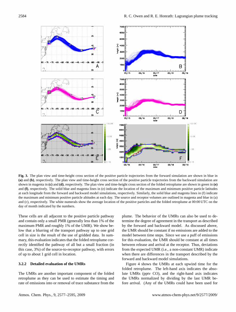
In contrast to the gridded output from the LPDM, the par-ticle trajectories and the folded retroplume offer a clear viewof the transport pathway between source and receptor. Fig-ure3 shows the plan view (a and c) and the time-height crosssection (b and d) of the positive particles from the forward (aand b) and backward (c and d) model simulations. Figure3eand f shows the plan view and the time-height cross section,respectively, of the folded retroplume pathway obtained fromfolding the two model simulations using Eq. (4).

In terms of the core transport pathway described by thethree products, there was good overall agreement in both thehorizontal and vertical pathways. All indicated lofting ofemissions to 1–2 km in a daytime BL during the first fewhours of transport. The emissions remained at this altitude,after the transition from a deeper continental daytime BL toa shallow nighttime marine BL left them located in the FT.Once in the FT, the emissions experienced slower ascent toabout 3 km for approximately 1 day, where they remained foranother day. Finally, during the last 2 days of transport, theemissions experienced a gradual descent from 3 km to the re-ceptor at 2–2.25 km. The horizontal pathway shows that theemissions traveled northward along the coast to Nova Sco-tia, then traveled southeast before heading northeast again,toward the receptor. The common transport described by all

three products indicates that the folded retroplume success-fully identifies the large-scale transport pathway between thesource and receptor.

A comparison of the positive particle and folded retro-plume pathways reveals three interesting features outside ofthe core transport pathway. Two of these features are regionswhere, due to the random components of the model, the path-ways of the forward and backward positive particles differ.One such situation occurs during the initial day of transport(15–16 May) during the ascent from 1 km to 3 km (abovethe core transport pathway shown in panels b and d). Theforward and backward maximum particle locations indicatedin panel f encompass this region, indicating it is part of thesource-to-receptor transport pathway. However, the smallernumber of particle trajectories indicate that the probabilityof transport though this region is very low. The folded retro-plume correctly identifies this low-probability region with afairly small PMR, colored with darker greens and black. Thesecond region where there is a difference between the for-ward and backward particle trajectories occurs during the lasthalf of 16 May, when two forward positive particles straybelow the core transport region (panel b). The very smallnumber of trajectories from the forward model here indicatesthat this region is not part of the primary source-to-receptortransport pathway. The third feature is the presence of a fewcells with a non-zero PMR that are entirely outside the limitsof the positive particle pathway (i.e., a false positive PMR).



Fig. 3. The plan view and time-height cross section of the positive particle trajectories from the forward simulation are shown in blue in(a) and(b), respectively. The plan view and time-height cross section of the positive particle trajectories from the backward simulation areshown in magenta in(c) and(d), respectively. The plan view and time-height cross section of the folded retroplume are shown in green in(e)and(f), respectively. The solid blue and magenta lines in (e) indicate the location of the maximum and minimum positive particle latitudesat each longitude from the forward and backward model simulations, respectively. Similarly, the solid blue and magenta lines in (f) indicatethe maximum and minimum positive particle altitudes at each day. The source and receptor volumes are outlined in magenta and blue in (a)and (c), respectively. The white numerals show the average location of the positive particles and the folded retroplume at 00:00 UTC on theday of month indicated by the numbers.

These cells are all adjacent to the positive particle pathwayand contain only a small PMR (generally less than 1% of themaximum PMR and roughly 1% of the UMR). We show be-low that a blurring of the transport pathway up to one gridcell in size is the result of the use of gridded data. In sum-mary, this evaluation indicates that the folded retroplume cor-rectly identified the pathway of all but a small fraction (inthis case, 3%) of the source-to-receptor pathway, with errorsof up to about 1 grid cell in location.

3.2.2 Detailed evaluation of the UMRs

The UMRs are another important component of the foldedretroplume as they can be used to estimate the timing andrate of emissions into or removal of trace substance from the

plume. The behavior of the UMRs can also be used to de-termine the degree of agreement in the transport as describedby the forward and backward model. As discussed above,the UMR should be constant if no emissions are added to themodel between time steps. Since we use a puff of emissionsfor this evaluation, the UMR should be constant at all timesbetween release and arrival at the receptor. Thus, deviationsfrom the expected UMR (i.e., a non-constant UMR) indicatewhen there are differences in the transport described by theforward and backward model simulations.

Figure 4 shows the UMRs at each upwind time for thefolded retroplume. The left-hand axis indicates the abso-lute UMRs (pptv CO), and the right-hand axis indicatesthe UMRs normalized by dividing by the last UMR be-fore arrival. (Any of the UMRs could have been used for



Fig. 4. Upwind mixing ratios (UMRs) at each transport time be-tween departure at the source and arrival at the receptor for theevaluation simulation. The bottom axis indicates the date while thetop axis indicates the upwind day number. The left-hand axis indi-cates absolute UMRs and the right-hand axis indicates the relativeUMRs, normalized by the last UMR. Numbers and vertical dottedlines indicate periods discussed in detail in the text.

normalization, but we chose this value because there hasbeen little deformation of the air mass between the sampletime and the arrival time in the receptor due to the calm me-teorological scenario. As a result, it should closely representthe UMR that would be calculated if the forward simulationcould be sampled while in the receptor cell.)

There are clearly significant variations in the UMR val-ues, approximately 35% in the negative direction and a lit-tle more than 45% in the positive direction. We considertwo possible causes for these deviations. These deviationscan be the result of irreversibility, which would indicate thatthe forward and backward simulations are not simulating thesame transport. Irreversible transport can be caused by oneor more of a number of factors, including the violation ofthe well-mixed criterion (Thompson, 1987), not maintain-ing a consistent representation of the mass of particles asair density changes (Lin et al., 2003), and errors induced bythe interpolation of meteorology between grid points (Stohl,1998). The two positive particles that stray from the primarytransport pathway and do not coincide with positive back-ward particles may indicate that a small portion of this eventis irreversible. However, the overall agreement between theforward and backward positive particle trajectories indicatethat the primary transport pathway described for this event isreversible. Another source of these deviations could be thepresence of sub-grid gradients in the CO or sensitivity fieldthat are lost when gridded fields are calculated. In order toinvestigate this potential, we conducted detailed inspectionsof the CO concentrations, sensitivity, and PMR fields andthe distributions of the positive and negative particles in thevicinity of the positive particles at several times, marked bythe dotted vertical lines in Fig.4.

This investigation determined that the low UMRs resultedfrom minor displacements (less than the size of a grid cell)between the groups of forward and backward positive parti-cles, specifically in regions with a high mixing ratio or sensi-tivity gradient. For the transport scenario examined here, theforward CO plume near the receptor (time period 4 in Fig.4)is a thin filament, on the order of 2–4 grid cells wide, and thepositive forward particles are at the edge of this filament ofCO (only the part of the CO plume that contains positive par-ticles actually passes through the receptor cell). Thus, whenthe positive backward particles are displaced slightly fromthe positive forward particles, they are in a region with littleCO, resulting in a very small PMR in those cells and a nega-tive bias in the calculated UMR. A similar case can be foundin period 3.

Around period 2, the roles of the sensitivity and CO plumebegin to change. Around this time, the sensitivity plumesplits (as it is followed backward in time), with one portionheading northeast and another portion (which contains thepositive particles) heading southwest, towards the receptor.Meanwhile, the CO plume (as it is tracked forward in time)is also in the process of splitting in two. One portion is the fil-ament that eventually travels to the receptor, and the other isthe larger portion that travels northeast from the source. Thepositive forward and backward particles were still slightlydisplaced from one another. However, they were no longerlocated at the edge of their respective plumes, and thus nolonger in a region of a high sensitivity or CO gradient. Asa result of these conditions, the UMRs around this time arecloser to the expected value.

Closer to the source region, however, a different situationresults in UMRs with a positive bias. First, there is again alarge CO gradient (as in the other periods). However, nowthere is a relatively large concentration of negative forwardparticles in these cells, because the plume has not dispersedmuch yet. Second, the sensitivity plume was more dispersed.The positive backward particles reside in more cells and aredistributed more uniformly than the positive forward parti-cles. As a result of the these two factors, the positive back-ward particles are located in cells with a large number ofnegative forward particles. The sensitivity plume is there-fore combined with significantly higher CO, resulting in ahigher UMR. As the trace substance will be ubiquitous verynear source regions in most model scenarios, this situationmay occur frequently when UMRs are calculated close to thesource region.

3.3 The impact of various model settings on the foldedretroplume

Many model settings can affect how well transport is de-scribed, affecting the correlation between model simula-tions. Additionally, the way in which the output is savedcan affect the number of positive and negative particles thatare identified as being colocated. As the evaluation above



Table 1. Model settings used for evaluation.

Parameter name Setting options

Averaging On and off1

Temporal output interval 11, 3, and 6 hSpatial output grida 0.5◦1, 1.0◦, and 2.0◦

Kernel On and off1

Internal model time step ifine and ctl 5 and 201,b

Number of forward particlesc 75 000d and 500 0001,e

Number of backward particlesc 2500f and 20 0001,g

1 Identified as preferred model settings for folded retroplume.a Used for both latitude and longitude simultaneously.b Used for both ifine and ctl simultaneously.c High and low number of particle pairs only run together.d Resulted in 20–40 positive particles.e Resulted in 250–625 positive particles.f Resulted in 25–35 positive particles.g Resulted in 250–650 positive particles.

demonstrated, these factors can in turn significantly affectthe folded retroplume UMRs. We have evaluated the im-pact of the model settings listed in Table1 upon the foldedretroplume pathway and UMRs. We used the same releasescenarios used in the evaluation, with every possible combi-nation of the settings in Table1 (144 simulations in total) inorder to assess the impact of each model setting on the re-sulting folded retroplume pathway and UMRs. By runningall possible groupings for these settings, we are able to eval-uate the impact of changing one setting across all other pos-sible settings. The model settings that were identified as thebest settings (i.e., produced the most accurate pathway andUMRs) were used in the evaluation presented above. Here,we discuss the degree to which use of other model settingschanged the evaluation results.

3.3.1 Folded retroplume pathway

Across all the model settings, the folded retroplume pathwaywas qualitatively similar to the results presented in the eval-uation above. Larger output grid sizes naturally increasedthe size of the folded retroplume pathway, as the cells on theedge of the pathway were larger. The use of time-averagedoutput produced a mild ghosting effect, which is the super-position of negative particles that are located in the samecell but at different times during the averaging period. Thus,when averaged output was used, the folded retroplume path-way tended to be larger, with the occurrence of a few falsepositive PMRs along the edge of the transport pathway. De-spite these two issues, the resultant folded retroplume path-way correctly identified the core transport pathway taken bythe positive particle for all settings.

3.3.2 Folded retroplume UMRs

The general behavior of the UMRs were similar to thoseshown in Fig.4: lower near the receptor, highly variablefrom 1 to 2.5 days upwind, relatively flat at approximately3 days upwind, and very high at 4 days upwind, near thesource. The higher positive bias in the UMR near the sourceregion was present in all scenarios, indicating that no partic-ular setting can help resolve this issue. This is not surprising,given the cause of this issue discussed in Sect.3.2.2. The ab-solute value of the UMRs varied significantly with changesin the spatial size of the output grid, the frequency of out-put, and the use of average or instantaneous output, each ofwhich we discuss further below. However, the other threemodel settings (the number of particles, the sampling kernel,and the model time steps, ifine and ctl) had little impact onthe UMRs, and will not be discussed in detail. The num-ber of particles were chosen so that forward and backwardsimulations both had roughly 30 or 600 positive particles forthe small and large number of total particle sets, respectively.The lower number of particles was sufficient to return an ac-curate folded retroplume, which bodes well for future use ofthe method, as a lower number of particles can significantlydecrease the computational time necessary for the forwardsimulations.

3.3.3 Spatial grid sizes

The size of the spatial grids can affect how positive and neg-ative particles are associated with one another. A larger gridcell can either increase or decrease the UMR, depending onthe circumstances. For example, consider a cell that extendsvertically from the surface into the FT, in a case in whichthe pollution plume that would reach the receptor was trav-eling in the lower FT. This would result in all the positiveforward and backward particles residing in only the top halfof the cell. If this cell were over an emissions source, then thelower portion of the cell would have a large number of nega-tive forward particles, released from the surface source. Theuse of this single cell would result in a significant overesti-mate of the PMR, since the forward particles in the BL wouldbe included in the calculation. However, if this cell were notover an emissions source and the bottom half of the cell hadno forward particles, the result would be an underestimate ofthe PMR in this cell, as the larger cell would dilute the massof the positive forward particles over a larger region, givinga smaller mixing ratio, without affecting the sensitivity. Inour analysis, the resulting UMRs either stayed the same ordecreased by 5–10% with each increase in the grid cell size,though the decrease in the UMRs was more pronounced asthe grid cell size was increased from 1◦ to 2◦. Therefore, werecommend use of a grid size of 1◦

×1◦.



3.3.4 Averaged or instantaneous values and the lengthof averaging period

The folding method we propose depends on the colocationin both time and space of positive particles in order to suc-cessfully identify cells that contain the trace substance thatwill travel between the source and receptor. As noted inSect.3.3.1, time averaging produced a ghosting effect andproduced false positive PMRs. This ghosting effect also pro-duced a positive bias in PMRs within the folded retroplumepathway, when, over the course of the averaging period,an output grid cell spanned a region that included both theplume of interest (positive forward particles) and forward-model CO that did not ultimately reach the receptor (nega-tive forward particles). This could occur, for example, whena sensitivity plume was located along the edge of the COplume. The ghosting effect could cause the sensitivity plumeto sample portions of the center of the CO plume, resultingin higher UMRs. Longer averaging periods can increase thelikelihood that this ghosting effect can occur. At the short-est averaging period of 1 h, the averaged and instantaneousUMRs differed only slightly. The UMRs increased signifi-cantly as the length of the averaging period increased, withthe UMRs roughly doubling at all times at each time inter-val increase. If UMR values are to be used quantitatively,we recommend instantaneous fields over averaged fields fora folded retroplume. Instantaneous values, however, increasethe stochastic uncertainties of the output field. Since the 1 haveraged output and the instantaneous output were quite sim-ilar, a short averaging period (e.g., less than or equal to 1 h)may also be a good option, as the averaged fields will re-duce the stochastic uncertainties without affecting the UMRsgreatly.

3.4 Summary of evaluation

The transport pathway evaluation indicates that the foldedretroplume does a good job of restoring the source-to-receptor transport pathway and that this pathway is quite ro-bust over a variety of model settings. The UMR evaluation,however, indicates that large gradients in either the trace sub-stance or sensitivity field combined with minor differencesin transport can significantly impact the UMRs. We alsofound that the ubiquitous nature of the trace substance in thesource region in combination with a well-dispersed sensitiv-ity plume can lead to positive deviations in the UMRs. Theuse of larger grid sizes or an averaging period greater than1 h can significantly degrade the accuracy of the UMRs, re-sulting in bias (mainly positive).

One important result from the evaluation is that significantdeviations in the UMRs did not correlate with significant dif-ferences between the folded retroplume and positive particletransport pathways. Whether the UMRs were high or low, thecorrect cells were generally identified (i.e., the cells with pos-itive particles), with the core transport and fringe cells appro-

priately corresponding to high- and low-probability transportregions. As a result, the folded retroplume pathway appearsto be a robust product, even when differences in transportbetween the forward and backward model are indicated byvariations in the UMRs.

4 Sample application

In this section, we present a sample analysis that contraststhe folded retroplume method with traditional methods us-ing only standard gridded LPDM products. The analysis willserve to provide an example of the advantages of the foldedretroplume method over traditional LPDM analysis methods.The sample analysis will again focus on the transport of USemissions to the Pico Mountain observatory, examining thetransport scenario for an event observed at the Pico Moun-tain observatory from 21–23 April 2005. During the event,CO mixing ratios ranged from 120–180 ppbv, approximately30–90 ppbv above the typical springtime background at thestation, while FLEXPART indicated enhancements of 20–50 ppbv of CO. Ozone, nitrogen oxides, and non-methanehydrocarbons were also elevated during this period. Theevent is the second of two events discussed byHonrath et al.(2008).

As with the evaluation simulations, we use FLEXPARTversion 6.2, driven with ECMWF meteorological data, withNorth American CO emissions based on the EDGAR inven-tory (see Sect.3.1 for more details). For the sample analy-sis, we chose settings that are fairly typical of FLEXPARTapplications, even though they deviated somewhat from therecommendations above, especially in terms of the averag-ing period used. CO emissions were released continuouslyover North America into the lowest 300 m of the atmosphereand carried in the model for 20 days, after which time theywere dropped from the simulation. Particles for the back-ward simulation were released over a 1-h period centeredon 21:00 UTC on 21 April, into a box bounded by 38–39◦ N latitude 29–28◦ W longitude, from an altitude of 2000–2500 m a.s.l. The output was saved on a 1◦

×1◦ grid, with thetop of the output levels at 0.3, 1, 1.5, 2, 2.5, 3, 4, 5, 7.5, 10,and 15 km. 6-h averages were saved and the sampling ker-nel was used. Particle trajectories from the backward modelsimulation were also saved and were used to confirm that thefolded retroplume correctly captured the transport pathwayof emissions between the source and receptor during the last8 days of transport.

4.1 Comparison of the folded retroplume pathway withstandard LPDM products

The sensitivity plume (Fig.5a and c) shows fairly well or-ganized transport originating over the US west coast about7 days upwind. It also shows some sensitivity over a sec-ondary region in the Central US, from Texas to the Great



Fig. 5. The time-height cross section (a andb) and plan views (c andd) of the sensitivity plume (red, a and c) and the folded retroplume(green, b and d) for the sample analysis. The plan-view color scales are based on the maximum specific volume weighted residencetime (3.1 s m3 kg−1) and PMR (1.5 ppbv) for each plot. The white numerals show the average location of the sensitivity plume and foldedretroplume at each upwind day, as indicated by the numbers. The time-height cross sections are normalized by the maximum value at eachupwind time.

Lakes. Since the age of this secondary region is not apparent,snapshots of the sensitivity would be needed to determine itsage. The time-height cross section shows that the sensitiv-ity plume was in the lower levels of the atmosphere, whereit would be able to pick up emissions if they were present,from about 6.5 to 4 days upwind. At 4 days upwind, the bulkof the sensitivity plume experienced relatively rapid uplift tothe lower FT, where it stayed until arrival at the observatory.Thus, from these views of the sensitivity plume, one couldconclude that the bulk of emissions would have been pickedup during the leg of transport from the US west coast to Cen-tral, Northern US (i.e., between the 6 and 4 in Fig.5a). Amap of the source contributions (i.e.,

∑j Sj,t,(j ′,t ′)·Ej,t from

Eq.7, not shown) would show the true sources, primarily theCentral US and only partly from the US west coast. However,tracking the emissions once away from the primary sourceregion would be difficult due to the low sensitivity betweenthis region and the compact transport pathway that occursstarting from approximately 2.5 days upwind.

In contrast to the sensitivity plume, the transport leg fromthe west coast almost disappears in the folded retroplume(Fig. 5b), indicating this transport pathway actually carriesonly a small amount of the trace substance. The folded retro-plume shows that the emissions travel slowly northward inthe lower atmosphere from upwind day 7 to 2. At 2 days up-wind, all of the emissions were transported out of the BL intothe lower FT, significantly later than indicated by the sensi-tivity plume. During the last 2 days of transport, the folded

retroplume and sensitivity plume indicate virtually identicaltransport, which is not surprising since the sensitivity indi-cates little dispersion in the last 2 days of transport.

In order to examine the causes for the differences betweenthe standard and folded retroplume and to further demon-strate the utility of the folded retroplume, in Fig.6 we showsnapshots of the sensitivity plume (left column) and thefolded retroplume (right column) plotted with contours of thetotal column CO from the forward simulation (blue lines).Snapshots are shown for 7(a and b), 5(c and d), 4(e and f),and 3(g and h) days upwind. For consistency among theseplots, we have used the maximum sensitivity and PMR fromall 4 plots for the color scale maximum.

We have selected contour levels and color scales for Fig.6that approximate typical usage for the CO and sensitivityplumes (e.g.,Trickl et al., 2003), as some arbitrary selectionof these settings was required. In some cases, it may be pos-sible to adjust the contour levels and color scales such thatfeatures that were originally not apparent become visible.Often, however, this would result in confounding other areasof the figure. Additionally, adjusting these settings for eachsnapshot and product is not a realistic analysis approach andquite often would require the analyst to have a prior knowl-edge of the feature they are trying to identify (from, e.g., thefolded retroplume or particle trajectories). Thus, it is rea-sonable to assume that the features identified by the foldedretroplume but not the standard products, as presented here,would indeed be missed in most analyses of this type.



Fig. 6. The plan view of snapshots of the horizontally integrated sensitivity plume (red, left column) and the folded retroplume (green,right column) with forward CO contours (blue lines, left and right columns) at 7 (a andb), 5 (c andd), 4 (e and f), and 3 (g andh) daysupwind. Sensitivity plume color scale based on the maximum specific volume weighted residence time for all 4 plots (3.1 s m3 kg−1). Foldedretroplume color scale based on the maximum PMR for all 4 plots (1.5 ppbv). CO contours at 10, 20, 30, and 60% of the maximum columnCO for all 8 plots (400 mg/m2).



Fig. 7. The UMRs at each upwind time for the sample evalua-tion. The UMRs calculated using the appropriate CO age classes areshown in green, while the alternate UMRs calculated with the totalCO are shown are black. The cumulative CO distributions from theforward model (blue boxes) and the backward model folded withemissions (magenta crosses) are also shown.

At 7 days upwind (Fig.6a and b), there are significant dif-ferences between the sensitivity plume and the folded retro-plume. The region of sensitivity over the Western US andEastern Pacific (Fig.6a) completely disappears in the foldedretroplume (Fig.6b), while the region of sensitivity over theCentral US is emphasized, with relatively large PMRs. Con-sidering the overlap of the sensitivity plume over the CentralUS with the CO contours, the lack of CO in the western lobeof the sensitivity field, and the altitude of the primary portionof the sensitivity plume (Fig.5), this result is not surprising.However, it serves to demonstrate the cause for differencesbetween the sensitivity plume and the folded retroplume. Theemphasized area over the Central US with large PMRs, how-ever, is considerably larger than the area indicated by the sen-sitivity plume and extends to regions with relatively low COlevels (i.e., it extends beyond the area enclosed by the COcontours).

At 5 days upwind (Fig.6c and d), there remain signifi-cant differences between the sensitivity plume and the foldedretroplume. The eastern lobe of the sensitivity plume hasgrown larger. The western lobe of the sensitivity plume nowshows up in the folded retroplume, as it has picked up someemissions over the Western US. In the absence of selectivelypicking contours and color scales, it would be impossible toidentify the western lobe as contributing to CO transportedto the receptor, as the sensitivity plume and selected CO con-tours do not overlap.

By 4 days upwind (Fig.6e and f), the primary easternand secondary western lobes of the sensitivity plume andPMR fields have merged. A significant portion of the foldedretroplume is now outside the CO contours. (That is, thisfeature would be missed using the standard products shownin panel e or by using superimposed contours of the sensi-tivity plume and forward output alone, like those shown in

Fig. 1. A minimum CO contour level of 1% of the maximumwould be required to indicate that the sensitivity plume andCO fields overlap. However, if this level were used for allthe plots, then the sensitivity plume and CO contours wouldcompletely overlap at all upwind times shown in Fig.6,which would incorrectly indicate that all of the sensitivityplume carried emissions.)

By 3 days upwind (Fig.6g and h), the two lobes havealmost completely coalesced and the outline of the foldedretroplume and sensitivity plume are fairly similar, thoughthe colors indicate the distribution of the trace substancewithin the plume is still quite different than the distributionof the sensitivity field. The folded retroplume and sensitivityplume are virtually identical during the final 2 days of trans-port (shown in Fig.5), which is expected, as the sensitivityplume was very narrow during this period.

4.2 Folded retroplume UMRs

The UMR distribution, shown in Fig.7 (thick, green solidline marked with diamonds), can be used to identify detailsabout the addition of emissions to the plume. IncreasingUMRs indicate the time periods when emissions were be-ing added to the plume. The slope of the UMR line duringthis period indicates the rate at which emissions were added.Finally, constant UMRs indicate periods when the sensitiv-ity plume was not located over source regions. (Note thatif removal processes were included, decreases in the UMRwould identify times during which removal occurred, thoughthe interpretation of changes in the UMR would be compli-cated by the competition between emission and removal. SeeSect.5.3for a discussion on this topic.)

The distribution of the CO mixing ratio age classes in thereceptor, which can be derived from the forward model (blueline in Fig.7) and from the backward model (by folding thesensitivity plume with the emissions inventory, magenta linein Fig. 7), provide another means to determine the detailsabout the timing and rate of the addition of emissions to theplume. Therefore, a comparison of these distributions withthe UMRs can help evaluate how well the UMRs accomplishthis task by differentiating between changes in the UMRs thatresult from differences in transport and those that result fromemissions (and/or removal, were it used). Since the foldedretroplume samples the forward simulation, the UMR att

days upwind should equal the sum of the CO mixing ratioage classes from the forward model that are greater thant

days old:

UMRt≈

Af∑i=t

χt, (j ′), i, (8)

whereAf is the number of days the trace substance is carriedin the forward model,χt,(j ′),i is the CO mixing ratio of agei (in days) in the receptor cell (j ′), and the sum is over allavailable CO mixing ratio age classes in the cell.



The relatively small change in the UMRs and CO distri-butions from 0 ppbv to about 5 ppbv during 20 to 10 daysupwind indicates that, during this time, the majority of theplume was not over an emissions region. From 10 to 4 daysupwind, however, the UMRs (green) and sensitivity-derivedCO (magenta) increased by about 17 ppbv and the forwardCO increased by about 20 ppbv (about 62% and 72% of thefinal UMR, respectively). This increase indicates that this isthe time period when the plume was over the emission regionand CO was actively being added to the plume. Between 9and 4 days upwind, the emission rate was fairly constant, atabout 2 ppbv/day according to the UMRs. During the last3 days of transport, however, CO distributions are relativelyflat, indicating the plume was no longer in the emissions re-gion, in agreement with the location of the folded retroplumeshown in Figs.5 and6. The UMRs are also relatively flat be-tween days 3 and 2, closely following the sensitivity-derivedCO distribution. Between days 2 and 1, however, the UMRsincrease significantly, coming closer to the forward CO dis-tribution, and are flat again, following the CO from the for-ward simulation during the last day of transport.

In order to understand the differences between the UMRsand the forward CO mixing ratio distribution (23–24% fromupwind day 7 to 2), we conducted an inspection of the COplume, folded retroplume, sensitivity plume, and positiveparticles from the sensitivity plume during days 2–7 (notshown). This inspection revealed several features that, to-gether, explain these low UMRs. First, the positive particleswere not colocated with the areas with the maximum PMR,indicating minor differences in the transport between the for-ward and backward model simulations. Second, the gradientin the forward CO mixing ratio is fairly large over the areacovered by the folded retroplume (varying by about 40% inthe horizontal direction and about 85% in the vertical direc-tion). The evaluation in Sect.3 showed that in situations likethis, with a large gradient in either the sensitivity or tracesubstance plume, the UMRs can be sensitive to minor dis-placements in the positive particle locations.

The magnitude of the deviations of the UMR can be putinto perspective by considering the magnitude of the dis-agreement between the forward CO mixing ratio age classdistribution (blue line in Fig.7) and distribution derived fromfolding the sensitivity with the emissions inventory (magentaline in Fig. 7). The differences between the forward (blue)and backward (magenta) derived CO distributions is partiallythe result of the differences in transport described by thetwo model simulations (and partially the result of differencesin the number of particles used).Seibert and Frank(2004)showed that even with a short travel distance, the differencebetween the two can be in excess of 10%. The differencebetween the CO derived from the forward output and back-ward output convolved with the emissions inventory is notabnormal for FLEXPART, based on our own comparison ofthe two. (Our analysis consisted of a comparison of the totalCO mixing ratio obtained from the forward model to the CO

mixing ratio obtained from simulations of backward model,initiated at the Pico Mountain observatory, convolved withthe emissions inventory. The comparison included approx-imately 6000 CO mixing ratios, covering 2 years worth ofdata.) The UMRs are in fact bounded by the forward andbackward CO distributions, which are derived from estab-lished modeling methods. This suggests that the deviationsin the UMR during these times are reasonable.

Archiving the full spectrum of forward trace substance ageclasses can require a significant amount of storage space. Forthe example presented here, we saved CO age classes at a 6-h resolution for the whole Northern Hemisphere in order toappropriately match sensitivity and CO mixing ratios. (Thisone-month simulation required 15.5 GB of storage.) As a re-sult, it is preferable for storage reasons to save only the totalCO mixing ratio. To evaluate the effect that this would haveon the UMR results, we have included the UMRs resultingfrom PMRs calculated by folding the sensitivity plume withall available CO mixing ratio age classes. Thus, Eq. (5) be-comes

PMRj, t=Sj, t, (j ′, t ′)·

Af∑i=0

χj, t, i . (9)

These UMRs are shown in Fig.7 (black line marked withasterisks). They match the other UMRs quite well during thelast 10 days of transport. However, from upwind days 10 to20, there is an obvious positive bias in these UMRs, result-ing from the sensitivity being folded with CO that will bedropped from the forward model before it can be transportedto the receptor (i.e., the particles will reach the maximum ageallowed and will thus be dropped from the forward simula-tion). Since we are mainly interested in the last∼10 days oftransport, when the bulk of the emissions have been added tothe plume and transported to the receptor, this would not bean issue with the example presented here. Deviations of theUMRs of this kind are most likely to occur at the greatest up-wind times, when very old CO emissions can be folded withsensitivity many days upwind of the receptor.

5 Alternate backward LPDM combinations

The method we have presented uses the transport sensitivityfrom the backward formulation of a model to estimate the lo-cation and distribution of the trace substance in the forwardmodel that will eventually arrive at the receptor. This is onlyone of many potential applications that combine the trans-port sensitivity from a backward LPDM with gridded fieldsfrom a number of sources. The simplest example, given bySeibert and Frank(2004), is the convolution of the sensitiv-ity plume with an emissions inventory to determine the ageclass distribution of the mixing ratio of the trace substance inthe receptor cell. Here, we discuss a few possibilities that fo-cus on the calculation of UMRs and similar estimates of thephysical attributes of the sensitivity plume at upwind times.



5.1 Chemical transport models

UMRs calculated from the folding of a chemical transportmodel (CTM) with the backward LPDM would allow for anevaluation of the mixing ratios in the portions of the CTMsampled by the sensitivity plume. This would give an esti-mate of the chemical transformations occurring in the CTMfrom the Lagrangian perspective provided by the sensitiv-ity plume and would provide insight into the chemical andtransport processes in the CTM. A similar application, inwhich the adjoint of transport was used to sample a CTM wasgiven byVukicevic and Hess(2000) andHess and Vukicevic(2003). Vukicevic and Hess(2000) determined the adjointof the CTM HANK to find the transport sensitivity of a non-reactive trace substance. These sensitivity fields were equiv-alent to those obtained from a backward LPDM.Hess andVukicevic (2003) then folded the adjoint sensitivity fieldswith output fields from the forward mode of the CTM tocompute UMRs (or, as described byHess and Vukicevic(2003), the sensitivity-weighted average of these fields).

In order to calculate UMRs from a CTM, ideally, the ad-joint of transport in the CTM would be used because trans-port would be described the same in both model directions.However, the backward LPDM is also an attractive alter-native, particularly when the adjoint of the CTM is not al-ready available. The UMRs calculated in this manner willequal the mixing ratio in the receptor if the LPDM and CTMtransport are sufficiently similar, no emissions are added, nochemistry occurs, and, if a passive trace substance is usedin the LPDM, no removal has occurred within the plume.The agreement of transport between the CTM and LPDMcould be tested by comparing forward model simulations us-ing a passive trace substance and identical emissions sources.Changes in UMRs over time can thus be used to evaluate thenet impact of emissions, removal and chemistry in the CTMfrom a Lagrangian perspective.

5.2 Meteorological fields, measurement and satellitedata, and other applications

Other potential applications exist, since any data that areavailable on a 3-D grid can be combined with the back-ward LPDM to calculate sensitivity-weighted fields. Such3-D data include meteorological fields, high-resolution mea-surements, and satellite data. Folding meteorological fieldswith the backward LPDM sensitivity provides the sensitivity-weighted upwind meteorological conditions for the sensitiv-ity plume (e.g., the average temperature of the plume at eachupwind time). This could be useful for determining the phys-ical conditions of the air that will ultimately reach the recep-tor, which can be used to drive chemical reactions in a La-grangian box model (e.g.,Evans et al., 2000).

UMRs calculated from atmospheric measurements pro-vide an additional estimation of the chemical and physicalproperties of a plume upwind of a receptor. Fields of at-

mospheric composition derived from satellite observations orfrom intensive in-situ aircraft sampling could be analyzed byfolding with the backward LPDM results to obtain UMRs. Inthese cases, the evolution of the air mass could be examinedas it traveled to the receptor by comparing the UMRs overtime.

5.3 Wet and dry removal

The discussion of the method has thus far focused only onsimulations that do not include any removal processes (i.e.,passive trace substances). The inclusion of removal pro-cesses, however, has important and interesting implicationsbut requires careful consideration. Generally, removal shouldeither be included or excluded in both of the paired modelsimulations. By comparing the UMRs from two sets of sim-ulations – one from two simulations with no removal (sub-scriptnr – UMRnr ) and one from two simulations with re-moval (subscriptwr – UMRwr ), the timing of removal canbe determined. For example, consider UMRs calculated atthree time periods, one close to the source,ts , one near thereceptor,tr , and an intermediate time,ti . If no emissions areadded to the air mass fromts to tr , then UMRnr will be con-stant at all three times. However, if removal occurs betweeneither ts and ti or ti and tr , then UMRwr will decrease af-ter the removal has occurred. Therefore, a comparison of thetwo UMRs will indicate the timing of removal. Once the tim-ing has been determined from this method, the PMRwrs canbe compared with the PMRnrs to identify where this removaloccurred.

6 Practical considerations

There are a number of practical considerations relating to themodel settings and parameters that should be taken into ac-count when creating folded retroplumes. Two of the mostimportant of these are discussed in this section and are ex-pected to be of the greatest interest to readers wanting toconduct their own calculations of this type. This discussionis limited to the LPDM FLEXPART, but may be applied toother similar models by analogy.

6.1 FLEXPART output time stamp

In FLEXPART, the output is saved at the end of the averagingperiod. The forward and backward model simulations, how-ever, are integrated in opposite directions in time. Thus, ifaveraged (normal) output is used, in order to appropriatelymatch the model output, the length of the output intervalmust be added to the backward model output times, beforeidentical forward and backward times are selected for fold-ing.



6.2 Output unit options

The derivation presented in Sect.2.1used the volume mixingratio and a form of the sensitivity that also has units of mixingratio. Neither of these units are native to FLEXPART. Here,we discuss native FLEXPART output units that can be paired,along with some conversion factors, to obtain UMR units ofvolume mixing ratio. One such pairing is the mass missingratio for the forward mode (with model settings indsource=1and indreceptor=2) and the residence time from the back-ward mode (indsource=1 and indreceptor=1). In this case,the conversion factor necessary to obtain volume mixing ra-tios are the ratio of the mass of air to the mass of the tracesubstance (which serves to convert the mass mixing ratioto the volume mixing ratio) and the inverse of output inter-val (which serves to convert the residence time to the mix-ing ratio sensitivity). (Note, the inverse of the output inter-val may or may not be necessary with instantaneous out-put, depending on how the modifications are made to themodel code.) Another pair of native FLEXPART output unitsis concentration from the forward mode (indsource=1 andind receptor=1) and the specific volume weighted residencetime (SVWRT, indsource=1 and indreceptor=2). The con-version factors are identical to the first pair, the ratio of themass of air to the mass of the trace substance and the the in-verse of output interval.Seibert and Frank(2004) andStohlet al.(2005) review other potential model outputs.

7 Summary and conclusions

This paper introduced a new method, the product of whichwe call a folded retroplume, that identifies source-to-receptortransport pathways using standard gridded products from aLagrangian particle dispersion model (LPDM). The foldedretroplume can be used to determine the transport pathwayof only those emissions that arrive at the receptor at a desig-nated time and to estimate the timing and location of emis-sion and removal processes within the model.

An evaluation was conducted to determine the abilityof the folded retroplume to identify the source-to-receptortransport pathway and to consistently calculate the expectedsensitivity-weighted mixing ratios (upwind mixing ratios orUMRs) along the transport pathway. A comparison of thefolded retroplume pathway with particle trajectories fromboth the forward and backward LPDM simulations showedthat the folded retroplume was consistently able to repro-duce the source-to-receptor transport pathway across a widevariety of model settings. Minor differences between thefolded retroplume and particle pathways along the edge ofthe core transport pathway were found, but were limited toone or two grid cells (typically 10–100 km), a fairly minordifference when compared to the length of the transport path-way analyzed (3620 km). The UMRs may be expected tobe constant at all times between the source and receptor in

the evaluation simulations. However, significant variationsin UMRs were found to occur across all model settings. Thebest model settings produced UMRs that typically deviatedfrom the expected value by 20–40%, while other model set-tings produced deviations exceeding 100%. These deviationsresulted primarily from errors induced by using gridded datawhen large gradients in the trace substance and sensitivityfields were present and as well as minor differences betweenthe source-to-receptor transport described by the forward andbackward model simulations. The test simulations, however,provided a rather rigorous test of the folded retroplume prop-erties, particularly the UMRs, as the evaluation transport sce-nario produced high gradients.

A sample analysis of the transport of North American COto a monitoring station located in the Azores Islands con-trasted the folded retroplume with traditional LPDM analy-sis tools. The folded retroplume made it possible to identifytransport features that were difficult or impossible to deter-mine with the traditional LPDM analysis techniques. TheUMRs proved to be useful as a tool to determine the tim-ing and rate at which emissions were added to the plume.Had the sample analysis included removal processes, the tim-ing and rate of removal could also have been determined.We conclude that the folded retroplume is better than tra-ditional LPDM analysis techniques for determining source-to-receptor pathways because it is significantly easier andmore accurate than the alternative (separately viewing all thecomponents of the LPDM). The folded retroplume also pro-vides information unavailable from traditional LPDM prod-ucts, such as the location and timing of removal processesand the spatial distribution of the trace substance betweenthe source and receptor.

The large deviations of the UMRs in the evaluation raisedthe issue of the reversibility of the transport scenario. Eventhough it was ultimately determined that the transport sce-nario was reversible, the issue of the reversibility of any par-ticular transport scenario is important. While large variationsof the UMR can occur under certain conditions even in theabsence of irreversibility (as discussed in Sect.3.2.2), UMRsthat behave as expected indicate that the source-to-receptortransport pathway is correct and that the transport simulationwas reversible. The example transport scenario presented inSect.4 serves to illustrate this idea. The UMRs in the ex-ample were within the bounds of the corresponding equiva-lent mixing ratios calculated from the forward and backwardsimulations, and the folded retroplume pathway was foundto agree well with the positive particle trajectories from thebackward simulation. Thus, UMRs may provide a meansto determine when to accept the source-to-receptor transportpathway indicated by the folded retroplume as correct. Inthis respect, the folded retroplume may be superior to botha backward simulation and particle trajectories, neither ofwhich offers a means to determine reversibility of the trans-port scenario.



The folded retroplume should be most useful for the analy-sis of measurements made in relatively remote regions of theatmosphere, where pollution impacts result from emissionsthat have traveled long distances. In these cases, emissionsare often significantly dispersed, and the source-to-receptorpathway may be difficult to discern from standard LPDMproducts. This scenario is relatively typical of many mon-itoring stations (e.g.,Carpenter et al., 1997andKentarchoset al., 2000) and aircraft-based sampling efforts (e.g.,Cooperet al., 2001andLewis et al., 2007).

The LPDM folding technique can also be applied using thebackward LPDM to sample fields of mixing ratios, concen-trations, and meteorological data from other sources in orderto explore gridded data fields in a Lagrangian framework.When paired with the concentration output from a CTM, themethod could be used to probe the chemistry occurring in theCTM within the confines of the sensitivity plume. Appliedto satellite or field measurements, the method could be usedto examine the chemical and physical evolution of a plumein the atmosphere. Meteorological conditions extracted withthe method could be used to understand the conditions expe-rienced by an air mass during transport and can be used in atrajectory chemical transport model or box model. These al-ternate applications of the technique offer new opportunitiesto study physical and chemical transformations that occur inthe atmosphere.

Acknowledgements.We thank D. Henriques, Institute of Me-teorology, Ponta Delgada, Portugal, for providing the ECMWFdata used in this work and Andreas Stohl, Norsk Institutt forLuftforskning (NILU), Kjeller, Norway for providing the FLEX-PART model and assisting in its use. We also with to thank thereviewers, especially P. Seibert, for their suggestions for improvingthe manuscript. This research was supported by grants from theNational Science Foundation (ATM-0535486 and ATM-0720955).

Edited by: A. Stohl

References

Carpenter, L. J., Monks, P. S., Bandy, B. J., Penkett, S. A., Gal-bally, I. E., and Meyer, C. P.: A study of peroxy radicals andozone photochemistry at coastal sites in the northern and south-ern hemispheres, J. Geophys. Res., 102, 25417–25427, 1997.

Cooper, O., Moody, J., Parrish, D., Trainer, M., Ryerson, T., Hol-loway, J., Hubler, G., Fehsenfeld, F., Oltmans, S., and Evans,M.: Trace gas signatures of the airstreams within North Atlanticcyclones: Case studies from the North American Regional Ex-periment (NARE ’97) aircraft intensive, J. Geophys. Res., 106,5437–5456, 2001.

Cooper, O., Stohl, A., Eckhardt, S., Parrish, D., Oltmans, S., John-son, B., Nedelec, P., Schmidlin, F., Newchurch, M., Kondo,Y., and Kita, K.: A springtime comparison of troposphericozone and transport pathways on the east and west coasts ofthe United States, J. Geophys. Res., 110, D05S90, doi:10.1029/2004JD005183, 2005.

ECMWF: Users guide to ECMWF products 4.0, Tech. Rep. Mete-orological Bulletin M3.2, European Center for Medium-RangeWeather Forecasts (ECMWF), Reading, UK, 2005.

Errico, R. M.: What is an adjoint model?, B. Am. Meteorol. Soc.,78, 2577–2591, 1997.

Evans, M., Shallcross, D., Law, K., Wild, J., Simmonds, P., Spain,T., Berrisford, P., Methven, J., Lewis, A., McQuaid, J., Pilling,M., Bandy, B., Penkett, S., and Pyle, J.: Evaluation of a La-grangian box model using field measurements from EASE (East-ern Atlantic Summer Experiment) 1996, Atmos. Environ., 34,3843–3863, 2000.

Flesch, T., Wilson, J., and Yee, E.: Backward-Time LagrangianStochastic Dispersion Models and Their Application to EstimateGaseous Emissions, J. Appl. Meteorol., 34, 1230–1332, 1995.

Han, Y.-J., Holsen, T. M., Hopke, P. K., and Yi, S.-M.: Comparisonof back-trajectory based modeling and Lagrangian backward dis-persion modeling for location sources of reactive gaseous mer-cury, Environ. Sci. Technol., 23, 1715–1723, 2005.

Hess, P. and Vukicevic, T.: Intercontinental transport, chemi-cal transformations, and baroclinic systems, J. Geophys. Res.,108(D12), 4354, doi:10.1029/2002JD002798, 2003.

Honrath, R., Helmig, D., Owen, R., Parrish, D., and Tanner, D.:Non-methane hydrocarbons (NMHC) at Pico Mountain, Azores:2. Eevent-specific analysis of the impacts of mixing and photo-chemistry on hydrocarbon ratios, J. Geophys. Res., 113, D20S92,doi:10.1029/2008JD009832, 2008.

Kentarchos, A. S., Roelofs, G. J., Lelieveld, J., and Cuevas, E.:On the origin of elevated surface ozone concentrations at IzanaObservatory, Tenerife during late March 1996, Geophys. Res.Lett., 27, 3699–3702, 2000.

Lehmann, R., von der Gathen, P., Rex, M., and Streibel, M.: Sta-tistical analysis of the precision of the Match method, Atmos.Chem. Phys., 5, 2713–2727, 2005,http://www.atmos-chem-phys.net/5/2713/2005/.

Lewis, A. C., Evans, M. J., Methven, J., Watson, N., Lee, J. D.,Hopkins, J. R., Purvis, R. M., Arnold, S. R., McQuaid, J. B.,Whalley, L. K., Pilling, M. J., Heard, D. E., Monks, P. S., Parker,A. E., Reeves, C. E., Oram, D. E., Mills, G., Bandy, B. J., Stew-art, D., Coe, H., Williams, P., and Crosier, J.: Chemical compo-sition observed over the mid-Atlantic and the detection of pollu-tion signatures far from source regions, J. Geophys. Res., 112,D10S39, doi:10.1029/2006JD007584, 2007.

Lin, J., Gerbig, C., Wofsy, S., Andrews, A., Daube, B., David,K., and Grainger, C.: A near-field tool for simulating the up-stream influence of stmospheric observations: The StochasticTime-Inverted Lagrangian Transport (STILT) model, J. Geophys.Res., 108(D16), 4493, doi:1029/2002JD003161, 2003.

Methven, J., Arnold, S., O’Connor, F., Barjat, H., Dewey, K., Kent,J., and Brough, N.: Estimating photochemically produced ozonethroughout a domain using flight data and a Lagrangian model,J. Geophys. Res., 108(D9), 4271, doi:10.1029/2002JD002955,2003.

Methven, J., Arnold, S., Stohl, A., Evans, M., Avery, M., Law,K., Lewis, A., Monks, P., Parrish, D., Reeves, C., Schlager,H., Atlas, E., Blake, D., Coe, H., Crosier, J., Flocke, F.,Holloway, J., Hopkins, J., McQuaid, J., Purvis, R., Rap-pengluck, B., Singh, H., Watson, N., Whalley, L., and Williams,P.: Establishing Lagrangian connections between observationswithin air masses crossing the Atlantic during the Interna-


http://www.atmos-chem-phys.net/5/2713/2005/


tional Consortium for Atmospheric Research on Transport andTransformation experiment, J. Geophys. Res., 111, D23S62,doi:10.1029/2006JD007540, 2006.

Neuman, A., Parrish, D., Trainer, M., Ryerson, T., Holloway, J.,Nowak, J., Swanson, A., Flocke, F., Roberts, J., Brown, S.,Stark, H., Sommariva, R., Stohl, A., Peltier, R., Weber, R.,Wollny, A., Sueper, D. T., Hubler, G., and Fehsenfeld, F.: Reac-tive nitrogen transport and photochemistry in urban plumes overthe North Atlantic Ocean, J. Geophys. Res., 111, D23S54, doi:10.1029/2006JD007010, 2006.

Olivier, J., Bouwman, A., der Maas, C. V., Berdowski, J., Veldt,C., Bloos, J., Visschedijk, A., Zandveld, P., and Haverlag, J.:Description of EDGAR Version 2.0: A set of global emissioninventories of greenhouse gases and ozone-depleting substancesfor all anthropogenic and most natural sources on a per countrybasis and on 1◦×1◦ grid, Tech. Rep. 771060 002 and R96/119,National Institute of Public Health and the Environment (RIVM)and Netherlands Organization for Applied Scientific Research(TNO), 1996.

Owen, R. C., Cooper, O. R., Stohl, A., and Honrath, R. E.: An anal-ysis of the mechanisms of North American pollutant transportto the central North Atlantic lower free troposphere, J. Geophys.Res., 111, D23S58, doi:10.1029/2006JD007062, 2006.

Rex, M., von der Gathen, P., Harris, N., Lucic, D., Knudsen, B.,Braathen, G., Reid, S., Backer, H. D., Claude, H., Fabian, R.,Fast, H., Gil, M., Kyro, E., Mikkelsen, I., Rummukainen, M.,Smit, H., Stahelin, J., Varotsos, C., and Zaitcev, I.: In situ mea-surements of stratospheric ozone depletion rates in the Artic win-ter 1991/1992: A Lagrangian approach, J. Geophys. Res., 103,5843–5853, 1998.

Seibert, P. and Frank, A.: Source-receptor matrix calculation with aLagrangian particle dispersion model in backward mode, Atmos.Chem. Phys., 4, 51–63, 2004,http://www.atmos-chem-phys.net/4/51/2004/.

Stohl, A.: Computation, accuracy and applications of trajectories –a review and bibliography, Atmos. Environ., 32, 947–966, 1998.

Stohl, A. and Trickl, T.: A textbook example of long-range trans-port: simultaneous observation of ozone maxima of stratosphericand North American origin in the free troposphere over Europe,J. Geophys. Res., 104, 30445–30462, 1999.

Stohl, A., Wotawa, G., Seibert, P., and Kromp-Klob, H.: Interpo-lation errors in wind fields as a function of spatial and temporalresolution and their impact on different types of kinematic tra-jectories, J. Appl. Meteorol., 34, 2149–2165, 1995.

Stohl, A., Eckhardt, S., Foster, C., James, P., Spichtinger, N., andSeibert, P.: A replacement for simple back trajectory calcula-tions in the interpretation of atmospheric trace substance mea-surements, Atmos. Environ., 36, 4635–4648, 2002a.

Stohl, A., Trainer, M., Ryerson, T. B., Holloway, J. S., and Parrish,D. D.: Export of NOy from the North American boundary layerduring 1996 and 1997 North Atlantic Regional Experiments,J. Geophys. Res., 107(D11), 4131, doi:10.1029/2001JD000519,2002b.

Stohl, A., Forster, C., Eckhardt, S., Spichtinger, N., Huntrieser, H.,Heland, J., Schlager, H., Wilhelm, S., Arnold, F., and Cooper, O.:A backward modeling study of intercontinental pollution trans-port using aircraft measurements, J. Geophys. Res., 108(D12),4370, doi:1029/2002JD002862, 2003.

Stohl, A., Cooper, O. R., Damoah, R., Fehsenfeld, F. C., Forster,C., Hsie, E.-Y., Hubler, G., Parrish, D. D., and Trainer, M.: Fore-casting for a Lagrangian aircraft campaign, Atmos. Chem. Phys.,4, 1113–1124, 2004,http://www.atmos-chem-phys.net/4/1113/2004/.

Stohl, A., Forster, C., Frank, A., Seibert, P., and Wotawa, G.: Tech-nical note: The Lagrangian particle dispersion model FLEX-PART version 6.2, Atmos. Chem. Phys., 5, 2461–2474, 2005,http://www.atmos-chem-phys.net/5/2461/2005/.

Thompson, A.: Criteria for the selection of stochastic models ofparticle trajectories in turbulent flows, J. Fluid Mech. , 180, 529–556, 1987.

Trickl, T., Cooper, O. R., Eisele, H., James, P., Mucke, R., andStohl, A.: Intercontinental transport and its influence on theozone concentrations over Europe: Three case studies, J. Geo-phys. Res., 108, 8530, doi:10.1029/2002JD002735, 2003.

Vukicevic, T. and Hess, P.: Analysis of tropospheric transport in thePacific Basin using the adjoint technique, J. Geophys. Res., 105,7213–7230, 2000.





technical note: a new method for the lagrangian tracking

Documents