technical rationale for changes to the method for … · web viewtechnical rationale for changes to...
TRANSCRIPT

Technical rationale for changes to the method for deriving Australian and New Zealand water quality guideline values for toxicantsPrepared for the revision of the Australian and New Zealand guidelines for fresh and marine water quality ReportOctober 2018

Technical Rationale for Changes to the Method for Deriving Australian and New Zealand Water Quality
Guideline Values for Toxicants
© Commonwealth of Australia 2018
Ownership of intellectual property rightsUnless otherwise noted, copyright (and any other intellectual property rights, if any) in this publication is owned by the Commonwealth of Australia (referred to as the Commonwealth).
Creative Commons licenceAll material in this publication is licensed under a Creative Commons Attribution 3.0 Australia Licence, except for photographic images, logos and the Commonwealth Coat of Arms.
Creative Commons Attribution 3.0 Australia Licence is a standard form licence agreement that allows you to copy, distribute, transmit and adapt this publication provided you attribute the work. See the summary of the licence terms or the full licence terms.
Inquiries about the licence and any use of this document should be emailed to [email protected].
Cataloguing dataThis publication (and any material sourced from it) should be attributed as: Batley, GE, van Dam, RA, Warne, MStJ, Chapman, JC, Fox, DR, Hickey, CW and Stauber, JL 2018. Technical rationale for changes to the Method for Deriving Australian and New Zealand Water Quality Guideline Values for Toxicants. Prepared for the revision of the Australian and New Zealand Guidelines for Fresh and Marine Water Quality. Australian and New Zealand Governments and Australian state and territory governments, Canberra, ACT, 49 pp.
AcknowledgementsThe authors gratefully acknowledge the valuable comments provided by the reviewers and discussions held with numerous colleagues during the development of the toxicant water guideline value derivation method.
ContactAustralian Government Department of Agriculture and Water ResourcesGPO Box 858 Canberra ACT 2601Switchboard +61 2 6272 3933 or 1800 900 090Email [email protected]
LiabilityThe authors of this publication, all other entities associated with funding this publication or preparing and compiling this publication, and the publisher of this publication, and their employees and advisers, disclaim all liability, including liability for negligence and for any loss, damage, injury, expense or cost incurred by any person as a result of accessing, using or relying on any of the information or data in this publication to the maximum extent permitted by law.
Australian and New Zealand Guidelines for Fresh and Marine Water Quality ii

Technical Rationale for Changes to the Method for Deriving Australian and New Zealand Water Quality
Guideline Values for Toxicants
ContentsContents.........................................................................................................................................iii
Modifications made since June 2014...............................................................................................iv
Summary.........................................................................................................................................v
1 Introduction.............................................................................................................................1
2 Definitions for acute and chronic toxicity.................................................................................2
2.1 Definitions for the Australian and New Zealand guidelines................................................2
3 Short- and long-term guideline values......................................................................................6
4 Acceptable test endpoints........................................................................................................7
5 Use of field, mesocosm and microcosm data............................................................................9
6 Hierarchy of acceptable statistical estimates..........................................................................11
7 Minimum dataset requirements for guideline value derivation..............................................13
8 Toxicity data inclusion rules and data quality assessment.......................................................17
8.1 Guideline value reliability.................................................................................................20
8.2 Selection rules for toxicity data to be used in species sensitivity distributions................24
8.3 Dealing with toxicity modifying factors............................................................................25
9 Analytical methods for deriving species sensitivity distributions.............................................28
10 Guidance on weighting of data in species sensitivity distributions..........................................30
11 Geographical/climate-specific considerations for species/data inclusion................................32
12 Uncertainties associated with guideline values.......................................................................34
Glossary........................................................................................................................................36
References....................................................................................................................................40
Australian and New Zealand Guidelines for Fresh and Marine Water Quality iii

Technical Rationale for Changes to the Method for Deriving Australian and New Zealand Water Quality
Guideline Values for Toxicants
Modifications made since June 2014
There have been a number of changes to the report since June 2014. Only technical changes are described below, minor edits are not included.
The citation of the report was changed.
Table 1: The content of the rows for acute microinvertebrates, chronic macroinvertebrates and chronic microinvertebrates were changed. Changes were made to the table notes, particularly the definitions of macroinvertebrates and microinvertebrates.Rows for three early life stages (lethality, development and fertilisation) have been added. Each row has its own definition of the minimum exposure duration to be considered chronic. The chronic section has been modified to accommodate both single- and multi-generation toxicity data and definitions of these terms are provided in the Glossary.
Section 7: Text has been added to the discussion on multimodal SSDs, and on combining fresh and marine chronic data.
Sections 8 and 9: Text has been added to the discussion on the log-logistic and Burr Type III distributions.
Section 8: Text has been added to the discussion on other factors affecting the reliability of guideline values.
Section 8.1: Text has been added to the discussion on bioaccumulating chemicals.
Section 8.3: Text has been added to the discussion on dealing with toxicity modifying factors.
Australian and New Zealand Guidelines for Fresh and Marine Water Quality iv

Technical Rationale for Changes to the Method for Deriving Australian and New Zealand Water Quality
Guideline Values for Toxicants
SummaryAs part of Phase 1 of the revision of the Australian and New Zealand Water Quality Guidelines for Fresh and Marine Water Quality (ANZECC/ARMCANZ 2000, referred to herein as the 2000 Guidelines), the Toxicants and Sediments Working Group was asked to investigate necessary revisions for the toxicant section. A workshop held at CSIRO Land and Water at Lucas Heights, NSW in April 2010 identified a range of tasks relating to methods for the derivation of guideline values (GVs) for toxicants (termed trigger values in the 2000 Guidelines). A contract to undertake these revisions was issued by the Council of Australian Government’s Standing Council on Environment and Water (SCEW) in February 2013. This report was prepared by CSIRO in consultation with selected expert members of the Toxicants and Sediments Working Group. This report provides the technical rationale for key changes to the derivation method. It supplements another report (Warne et al. 2018) that provides the full revised method for deriving toxicant GVs.
Key changes from the 2000 Guidelines that are discussed in this report include:
revised definitions of acute and chronic toxicity and altered classification of toxicity tests
macroalgal early life stage tests (ELS) (for example, fertilisation, germination and cell division) are now considered chronic
invertebrate ELS tests (for example, fertilisation and larval development) are now considered chronic
7-d juvenile or adult fish and amphibian mortality tests are now considered acute
advice on short- vs long-term toxicity
in toxicity testing, although some indication of repeatability is desirable, it is recommended that, rather than replication of concentrations, more concentrations should be obtained at the lower end of the concentration-response relationship (that is below a 50% effect) to reduce uncertainties and improve the precision of statistical estimates of toxicity
inclusion of non-traditional endpoints (for instance behavioural) allowed only if ecological relevance can be demonstrated
the acceptability of toxicity endpoints now follows the order NEC, EC/IC/LCx where x≤10, BEC10, EC/LC15–20, NOEC, and NOEC estimated from MATC, LOEC or LC50 values. The use of NOECs is discouraged in favour of ECx values
a revised hierarchy of dataset preferences when using species sensitivity distributions (SSDs) to derive GVs. These dataset preferences are: chronic data for ≥8 species (although an aspirational target is 15 species); chronic + converted acute data for ≥8 species; chronic data for 5–7 species; chronic + converted acute data for 5–7 species; converted acute data for ≥8 species or chronic freshwater + chronic marine data (only for organic chemicals); and converted acute data for 5–7 species.
updated Burrlioz software (version 2.0) is available that automatically uses a log-logistic distribution for <8 data points and the Burr Type III distribution for ≥8 data points
a new reliability classification for GVs has been developed and is based on: (i) the hierarchy of acceptable data, (ii) the sample size, and (iii) a visual estimation of goodness-of-fit. Very high reliability GVs have a good fit for ≥15 chronic data points. A good fit and ≥8 data points is classified as high reliability
Australian and New Zealand Guidelines for Fresh and Marine Water Quality v

Technical Rationale for Changes to the Method for Deriving Australian and New Zealand Water Quality
Guideline Values for Toxicants
guidance is provided on weighting of data in SSDs, geographical and climatic considerations and uncertainties associated with GVs.
The changes described herein detail specific revisions to the toxicant GV derivation method that incorporate national and international developments in science since 2000, such that the recommended procedures represent current best practice. In the areas discussed, the recommendations supersede earlier guidance, and where a conflict or inconsistency exists between this revision and earlier advice, the advice in this report and in the companion report that describes the full revised toxicant GV derivation method (Warne et al. 2018) takes precedence.
Australian and New Zealand Guidelines for Fresh and Marine Water Quality vi

Technical rational for changes to the Method for Deriving Australian and New Zealand Water Quality Guideline
Values for Toxicants
1 IntroductionThis document outlines changes to the methods for calculating water quality guideline values (GVs) for toxicants (termed trigger values in the 2000 Guidelines) in the Australian and New Zealand Guidelines for Fresh and Marine Water Quality in Document 4 of the National Water Quality Management Strategy (ANZECC/ARMCANZ 2000) and the rationale for the changes. In particular, it deals with methods for deriving GVs for toxicants in aquatic ecosystems as covered in Chapter 3 of Volume 1 and Chapter 8 of Volume 2 of the 2000 Guidelines. The changes update approaches to specific aspects of the 2000 Guidelines to incorporate national and international developments in science since the release of the 2000 Guidelines, such that the recommended procedures represent current best practice. In the areas discussed, the recommendations supersede any earlier guidance (ANZECC/ARMCANZ 2000, Warne 2001, Warne et al. 2013). The revised methodology is applicable for deriving both default (that is nationally-derived), site-specific and short-term GVs.
This report provides technical discussion on:
definitions for acute and chronic toxicity
short- and long-term GVs (previously termed trigger values)
acceptable test endpoints
use of field, mesocosm and microcosm data for deriving GVs
a hierarchy of acceptable statistical estimates
minimum dataset requirements for GV derivation
toxicity data inclusion rules and data quality assessment
analytical methods for constructing species sensitivity distributions (SSDs)
guidance on weighting of data in SSDs
geographical and climatic considerations
uncertainties associated with GVs.
Australian and New Zealand Guidelines for Fresh and Marine Water Quality 1

Technical Rationale for Changes to the Method for Deriving Australian and New Zealand Water Quality
Guideline Values for Toxicants
2 Definitions for acute and chronic toxicity
Defining acute and chronic toxicity, and determining which tests are to be considered chronic, is critical to the future development of water and sediment quality GVs (WQGVs and SQGVs) in Australia and New Zealand. A recent World Health Organisation (WHO) study (Hahn et al. 2014) showed that predicted no effect concentrations (PNECs) derived for five different chemicals varied by up to four orders of magnitude, partly due to lack of agreement on what constituted acute versus chronic toxicity. Clear definitions are critical because:
the magnitude of assessment factors (AF) used in deriving GVs, and in ecological risk assessments for chemicals, depends partly on the number of acute and chronic test data available, which in turn depends on how these tests are defined.
they affect the way acute and chronic data are combined to generate GVs and ‘safe’ dilutions for effluents.
it was not clear to users of the 2000 Guidelines whether certain tests should be defined as acute or chronic. It was evident that greater clarity was required both in the definition of acute and chronic toxicity, together with tabulation of the classification of particular test endpoints in relation to these definitions that can be used for deriving GVs.
2.1 Definitions for the Australian and New Zealand guidelinesThe 2000 Guidelines (ANZECC/ARMCANZ 2000) provided the following definitions of acute and chronic toxicity:
Acute toxicity: Rapid adverse effect (for instance death) caused by a substance in a living organism; can be used to define either the exposure or the response to the exposure (effect).
Chronic toxicity: Lingering or continuing for a long time; often for periods of several weeks to years; can be used to define either the exposure or the response to the exposure (effect). Chronic exposure typically includes a biological response of relatively slow progress and long continuance, often affecting a life stage.
More detailed discussions of particular endpoints were given in ANZECC/ARMCANZ (2000; Volume 2 Chapter 8.3, p. 91) and Warne (2001). For the purpose of deriving GVs, acute toxicity data used were of 24 to 96 h duration for multi-cellular organisms, and 24 to 72 h for single-celled organisms. However, this combined information did not cover all possibilities and led to confusion with respect to several common tests (for instance larval development tests) being classified as acute or chronic.
The terms acute and chronic have been retained, but re-defined as:
Acute toxicity: A lethal or adverse sub-lethal effect that occurs as the result of a short exposure period to a chemical relative to the organism’s life span.
Chronic toxicity: A lethal or adverse sub-lethal effect that occurs as the result of exposure to a chemical for a substantial proportion of the organism’s life span or an adverse effect on a sensitive early life stage.
Australian and New Zealand Guidelines for Fresh and Marine Water Quality 2
Technical Rationale for Changes to the Method for Deriving Australian and New Zealand Water Quality
Guideline Values for Toxicants
A substantial proportion of an organism’s lifetime would typically be greater than 10% (Newman 2010).
General guidance on what constitutes an acute versus a chronic endpoint and/or test is given in Table 1.
Table 1 Classification of acute and chronic toxicity tests for temperate species for the purposes of water quality guideline value derivation
TOXICITY TEST LIFE STAGEa RELEVANT ENDPOINTSb TEST DURATION
Acute
Fish and amphibians Adults/juveniles Allc <21 d
Embryos/larvae All <7 d
Macroinvertebratesd Adults/juveniles All <14 d
Embryos/larvae All (except fertilisation, larval development/ metamorphosis)
<7 d
Embryos/larvae Larval development/ metamorphosis
<48 h
Microinvertebratese Adults/juveniles/larvae All (except fertilisation and larval development—see microinvertebrate chronic)
<7 d
Macrophytes Mature All <7 d
Macroalgae Mature Lethality and growth <7 d
Microalgae Not applicable All ≤24 h
Microorganisms Not applicable All ≤24 h
Chronic
Fish and amphibians Adults/juveniles Allf ≥21 d
Embryos/larvae/eggs All ≥7 d
Macroinvertebrates Adults/juveniles/larvae All (except reproduction, larval development/metamorphosis/ fertilisation)
≥14 d
Adults/juveniles/larvae Reproduction ≥14 d (or at least 3 broods for large cladocerans)
Embryos Larval development/ metamorphosis
≥48 h
Gametes Embryo fertilisation ≥1 h
Microinvertebrates Adults/juveniles/larvae Reproduction ≥7 d (or at least 3 broods for small cladocerans)
Adults/juveniles/larvae Lethality/immobilisation ≥7 d
Embryo Larval development ≥48 h
Gamete Embryo fertilisation ≥1 h
Macrophytes Mature All ≥7d
Macroalgae Mature All ≥7 d
Early life stages Lethality ≥7 d
Early life stages Development ≥48 h
Australian and New Zealand Guidelines for Fresh and Marine Water Quality 3

Technical Rationale for Changes to the Method for Deriving Australian and New Zealand Water Quality
Guideline Values for Toxicants
TOXICITY TEST LIFE STAGEa RELEVANT ENDPOINTSb TEST DURATION
Early life stages Fertilisation ≥1 h
Microalgae Not applicable All >24 h
Microorganisms Not applicable All >24 h
a The life stage at the start of the toxicity test.
b Endpoints need to be ecologically relevant (see Section 4). c For acute tests, ‘All’ refers to all ecologically relevant endpoints for a particular life stage of a particular species.d Macroinvertebrates include invertebrates where full-grown adults are ≥2 mm long (for example decapods, echinoderms,
molluscs, annelids, corals, amphipods, larger cladocerans [such as Daphnia magna, Daphnia carinata and Daphnia pulex] and insect larvae of similar sizes).
e Microinvertebrates are defined here as invertebrate species where full-grown adults are typically <2 mm long. Examples of invertebrates that meet this criterion are some cladocerans (for example Ceriodaphnia dubia and Moina australiensis), copepods, conchostracans, rotifer, acari, bryozoa and hydra.
f For chronic tests, ’All’ encompasses all ecologically relevant endpoints measured in both single- and multi-generation tests.
Changes were made to the 2000 Guidelines based on current, ongoing and proposed usage of chronic versus acute toxicity. Major differences include:
macroalgal early life stage tests (ELS) (for example, fertilisation, germination and development) are now considered chronic
invertebrate ELS tests (for example, fertilisation and larval development) are now considered chronic
7-d juvenile or adult fish and amphibian mortality tests are now considered acute.
As previously, a minimum exposure duration of 24 h applies to acute toxicity tests to be used to derive GVs. However, shorter duration toxicity data (for instance short duration fertilisation tests; see Table 1) can be used under certain circumstances (see Section 3).
The recommended test durations in Table 1 apply to tests on temperate species, typically undertaken in water temperatures from 15–25oC. The challenge with rigid definitions such as these, is that there will be exceptions. For example, tropical organisms (tested at >25oC) develop much faster than temperate species and these are faster again than polar species. Consequently, chronic toxicity tests for tropical organisms may be of considerably shorter duration than for temperate species, while such tests for polar species (typically at 0oC for Antarctic and 5oC for sub-Antarctic) will be considerably longer than for temperate species. For example, a test on sea urchin development to pluteus larvae takes around 21 days for a polar species (King and Riddle 2001) compared to 72–96 h for a temperate species and 24–48 h for a tropical species (Rick Krassoi, Ecotoxicology Services Australasia, pers. comm., 2014). For example, tests on mortality and behavioural changes in polar ostracods, gastropods and amphipods can, in some species, run for up to 10 weeks (Catherine King, Australian Antarctic Division, pers. comm., 2014). These issues are not just restricted to climatic differences. The breadth of life histories associated with taxa represented by invertebrates means that it is not possible to make a general rule when defining chronic and acute test durations, hence invertebrates have been treated as two groups, microinvertebrates and macroinvertebrates (see Table 1). Similarly in the case of some vertebrates, the test durations listed as acute and chronic may not be appropriate, for example, some fish embryo chronic endpoints might be achieved in less than the specified 7 days. Given the above, it is likely that best professional judgement will be needed on
Australian and New Zealand Guidelines for Fresh and Marine Water Quality 4

Technical Rationale for Changes to the Method for Deriving Australian and New Zealand Water Quality
Guideline Values for Toxicants
some occasions to make a determination about whether a particular test should be regarded as acute or chronic. The basis for all professional judgement decisions must be transparent, understandable and documented.
Australian and New Zealand Guidelines for Fresh and Marine Water Quality 5

Technical Rationale for Changes to the Method for Deriving Australian and New Zealand Water Quality
Guideline Values for Toxicants
3 Short- and long-term guideline values
The 2000 Guidelines do not define either short- or long-term GVs as used in some jurisdictions, but rather recommended to protect ecosystems from long-term exposure to toxicants. Short-term (acute) exposure GVs could be derived for particular chemicals where there are sound test data that show that effects over short times are environmentally relevant. Such tests usually (but not necessarily) measure lethality and might be appropriate in cases of a spill event, or pulse exposures as can occur with pesticides in rivers, or where contaminants are short-lived and non-persistent due to dispersion, volatilisation or degradation. The minimum exposure period is generally 96 h, but there might be circumstances where a lesser exposure time is relevant. The types of tests considered to measure acute responses are detailed in Table 1.
If a short-term GV is required for a site-specific application, it can be derived using a species sensitivity distribution (SSD) applied to acute toxicity data. The preferred data order is: acute NEC, EC/IC/LC≤10, BEC10, EC/IC/LC15-20, and lastly NOEC data. However, if there are insufficient of those data then acute LC50/IC50/EC50, LOEC and MATC values should be divided by 5, 2.5 and 2, respectively, and used to estimate acute EC/IC/LC10 or NOEC values. If short-term GVs are to be used for non-guideline purposes such as setting licence conditions or in prosecutions then the data preferences may change to reflect the purpose of the GV. Advice on minimum datasets is provided in Section 7. No acute to chronic ratio (ACR) or default assessment factors (AFs) are applied to the acute data to derive short-term GVs, except for those used to convert the acute data to IC/EC/LC50 data. Apart from the use of acute toxicity data, the derivation process should follow the GV derivation method described in Warne et al. (2018). If necessary, additional guidance on short-term GVs could be sought from the Canadian protocol (CCME 2007).
Australian and New Zealand Guidelines for Fresh and Marine Water Quality 6

Technical Rationale for Changes to the Method for Deriving Australian and New Zealand Water Quality
Guideline Values for Toxicants
4 Acceptable test endpointsThe 2000 Guidelines stipulated that for GV derivation, only toxicity data that measured survival (including survival and immobilisation), growth and reproduction were acceptable. Biomarker data, such as biochemical endpoints or most behavioural data were not used, nor were data from commonly used bacterial bioluminescence assays used due to their lack of proven ecological relevance.
Canadian WQGVs (CCME 2007) use traditional endpoints (that is growth, reproduction and survival), as well as non-traditional endpoints (for example behaviour, predator avoidance, swimming ability, swimming speed and physiological/biochemical changes, including endocrine-disrupting ability) if their ecological relevance can be demonstrated, that is, whether the non-traditional endpoints influence a species’ ecological competitiveness and lead to an ecologically relevant negative impact (that is they affect traditional endpoints).
In the revised method, non-traditional endpoints such as biochemical and physiological responses are admissible for use in GV derivation, but only those based on in vivo testing where their ecological relevance can be demonstrated, that is, data from in vitro tests cannot be used. Non-traditional endpoints, including those for mutagenicity and genotoxicity, that have not had their ecological relevance unambiguously demonstrated, should only be used as an additional line of evidence in weight-of-evidence (WoE) based risk assessments. An argument for the inclusion of non-traditional endpoints can be made by the developer of a proposed GV, but the decision on whether it unambiguously demonstrates ecological relevance will need to be verified through an independent review process.
To demonstrate ecological relevance, behavioural endpoints, for example, need to show demonstrated links to growth, development and reproduction endpoints. Special consideration might be given to the use of behavioural endpoints if they are the only data available for unique environments, for example, polar, and this is discussed further in Section 11. It is noteworthy that a recent meta-analysis of the use of behavioural endpoints for aqueous exposures in aquatic toxicology, such as swim speed, distance moved, activity levels, spatial distribution patterns, feeding rates and courting events, found that they were generally similarly sensitive, and had similar or better detectable effect sizes and statistical power when compared to development and reproduction endpoints (Melvin and Wilson 2013). These results do not prove that these endpoints are ecologically relevant, but rather that they occur at similar concentrations.
Some papers have demonstrated links between photosynthetic and whole organism responses in microalgae and aquatic macrophytes, especially for certain herbicides (for instance Magnusson et al. 2008), but less so for metals. In particular, the Great Barrier Reef Marine Park Authority (GBRMPA) had tabulated these in some of its earlier Great Barrier Reef-specific guideline derivations (GBRMPA 2010), based on findings such as those of Cantin et al. (2007) on the effects of diuron on spawning of corals, although they were not officially adopted. For the current method, photosynthetic endpoints may be admissible for GV derivation as long as their ecological relevance can be demonstrated.
Australian and New Zealand Guidelines for Fresh and Marine Water Quality 7

Technical Rationale for Changes to the Method for Deriving Australian and New Zealand Water Quality
Guideline Values for Toxicants
A lack of effects data for single-celled non-algal microbial species (for example bacteria) in GV datasets in the 2000 Guidelines was noted. One way to measure microbial responses is via biochemical responses; however, biochemical responses do not, at this point, have sufficient proven ecological relevance and therefore they should not be used to derive GVs. Recent ecogenomic approaches in ecotoxicology, that quantify the functional genes of an entire biological population (micro-, meio- and macro-organisms), may in the future provide a better way of measuring ecologically relevant effects on biological communities, but currently they should not be used to derive default GVs. Their use for deriving regional or site-specific GVs should be appropriately justified.
In the derivation of GVs, the literature search should be restricted to data based on traditional endpoints, with data from non-traditional endpoints evaluated only in exceptional circumstances, for example, where there are insufficient traditional endpoints data, or to address particular site-specific concerns.
Australian and New Zealand Guidelines for Fresh and Marine Water Quality 8

Technical Rationale for Changes to the Method for Deriving Australian and New Zealand Water Quality
Guideline Values for Toxicants
5 Use of field, mesocosm and microcosm data
Mesocosms are large enclosures designed to mimic field exposure conditions. They take the form of large tanks, enclosures or artificial channels to mimic natural waterways, often, but not necessarily, located in or near water bodies. Microcosms are smaller laboratory-based bench-scale artificial ecosystems. Compared to laboratory-based ecotoxicity testing, field-based mesocosms enable long-term studies and permit the simultaneous evaluation of the effects of single contaminants on multiple taxonomic groups, including indirect effects such as predation and competition between species. Mesocosm studies also incorporate the effects of competing fate processes on contaminant bioavailability (Giesy et al. 1999). Because non-chemical stressors can also impact field responses, it is often difficult to establish cause-and-effect relationships in mesocosms.
The 2000 Guidelines indicated that the preferred data for deriving GVs is from multiple-species toxicity tests, that is, field or model ecosystem (mesocosm, microcosm, artificial stream) tests that represent the complex interactions of species in the field. Where such data were available, and where they met OECD requirements (OECD 1992), they were to be preferentially used in GV derivation. Many of these tests are, however, difficult to interpret and there were few such data available that met quality screening requirements. A single mesocosm study can provide data for 10–50 species (especially including ‘>’ values) and community metrics. Thus, a single study can carry significant weight compared with the rest of the individual species data. Examples include mesocosm studies of ammonia (Hickey et al. 1999) and metals (Hickey and Golding 2002, Clements et al. 2013). Where contaminant mixtures are involved, the integrated toxicity response is derived so the data are not useful for deriving thresholds for individual contaminants.
Consequently, most of the GVs in the 2000 Guidelines were derived using data from single-species toxicity tests, because these formed the bulk of the concentration-response information available (Chapman et al. 2001). For the revised method, collecting and reviewing papers containing field, mesocosm, microcosm, chronic EC10 data and papers containing LC50 data should be part of the data collection process for deriving GVs.
Despite the recommendations for the use of field-based, mesocosm and microcosm data in GV derivation, there have been few examples of these reported in the literature, probably due to the costs of undertaking such experiments. Chapman et al. (2001) reported the use of mesocosm toxicity data in combination with laboratory data to develop a site-specific GV for endosulfan in northern NSW.
The EU view (European Commission 2011) is that while field, mesocosm or microcosm data are not necessarily considered critical for deriving GVs, they can be used to corroborate the derived GVs. It is specifically stated in that document that ‘field and mesocosm data have an important role as lines of evidence in helping define the standard (guideline) (through helping reduce uncertainty)’, but these data would not be regarded as ‘higher tier’ data that would replace laboratory-based ecotoxicity data except for pesticides.
Australian and New Zealand Guidelines for Fresh and Marine Water Quality 9

Technical Rationale for Changes to the Method for Deriving Australian and New Zealand Water Quality
Guideline Values for Toxicants
If using field studies either for a site-specific investigation or to assist in GV derivation, the EU approach is to allow the local investigator to determine the preferred approach, noting the criteria for mesocosm data acceptance (European Commission 2011), which need to be considered in conjunction with the data quality assessment outlined in Table 2 (Section 8). These criteria for mesocosm data acceptance include, but are not restricted to:
an adequate and unambiguous experimental set-up, including a dosing regime that reflects; exposure in the field and measurement of chemicals
a realistic biological community
should be representative of the taxa distribution in the field should contain taxa that are sensitive to the toxicant’s mode of action
an adequate description of exposure pathways, especially in the compartment of interest, for example, water column
contaminant concentrations should be measured throughout the course of the experiment replenish the concentrations of any rapidly dissipating compounds
a sound statistical evaluation
selected sensitive endpoints should be in accordance with the mode of action of the toxicant
data should meet quality requirements and enable concentration-response curves for individual contaminants to be derived.
Unlike single species laboratory-derived toxicity data, field, mesocosm and microcosm data are likely to require significant additional analysis/interrogation before they are in a form ready for GV derivation. Any field, mesocosm and microcosm data should be carefully evaluated in relation to the above criteria before they are used to derive a GV, but should be acceptable provided they meet the quality criteria.
Verification of the level of protection afforded by laboratory-based toxicity testing remains an important use of field, mesocosm and microcosm data. Although the 2000 Guidelines promoted the use of field ecological data for deriving site-specific GVs, they provided little guidance on how to do this. van Dam et al. (2014) provided several examples about how this can be done, and also identified several recent methods that may be useful for using field data to derive GVs. This is an area that is receiving increasing attention (for instance Crane et al. 2007, Kwok et al. 2008, Hickey et al. 1999, Hickey and Golding 2002, Clements et al. 2013, Cormier and Suter 2013), although there are as yet no universally accepted methods for deriving GVs from these types of data. Additional information on the use of field effects data for deriving GVs is provided in ANZG (2018; http://www.waterquality.gov.au/anz-guidelines/guideline-values/derive/field-effects), in addition to guidance on using multiple lines of evidence for deriving GVs (http://www.waterquality.gov.au/anz-guidelines/guideline-values/derive/mloe).
Australian and New Zealand Guidelines for Fresh and Marine Water Quality 10

Technical Rationale for Changes to the Method for Deriving Australian and New Zealand Water Quality
Guideline Values for Toxicants
6 Hierarchy of acceptable statistical estimates
Much has been written recently about the acceptability of the no observed effects concentration (NOEC) as a useful measure in toxicity testing (for instance Chapman et al. 1996, Warne and van Dam 2008, Fox et al. 2012, Landis and Chapman 2011, Jager 2012, van Dam, Harford and Warne 2012). The case against NOECs has been well summarised by Newman (2008) and Fox et al. (2012), namely that the values are derived from an inappropriate application of hypothesis testing.
NOECs make up the majority of the toxicity data used in the derivation of toxicant GVs in the 2000 Guidelines. Consequently, it is likely to be some time before derivations solely using alternative estimates or measures can be undertaken. Nevertheless, in the short-term, the Australian and New Zealand GVs will move away from NOECs, to low effect concentrations, ECx, or inhibition concentrations, ICx (where x = 10–20% effect) as the preferred measure of toxicity, and for use in future GV derivations. The EC10 is defined as the estimated concentration causing a 10% effect compared to the control or an adverse effect on 10% of the organisms compared to the controls. This change is consistent with moves in other international jurisdictions (for example Environment Canada 2005, CCME 2007, USEPA 2009) away from the use of NOEC data to the use of model-based EC/ICx data.
It may be possible to interrogate existing datasets from which NOECs were determined, in order to derive EC/IC10 values, although the magnitude of this task can be significant, and is only likely to be undertaken on an as needs basis by specific users. A further limitation is that, in the vast majority of cases, the raw data needed to permit the calculation of ECx values from NOEC values are not presented in papers. Although the use of EC5 and EC10 values has been recommended, the latter are preferable given the greater errors and the increased likelihood that extrapolation rather than interpolation will be used to calculate EC5 values.
There have been several attempts to compare EC10 values with NOECs, despite the recognition that they are statistically not analogous (for instance Shieh et al. 2001, Green et al. 2013). The comparisons were more out of a desire to see how the numerical values relate to one another. The results of such comparisons will depend on the statistical model used, the endpoint (for example, growth, biomass), the number of data points used in the toxicity test, and the uncertainty associated with the endpoint. For example, Green et al. (2013), acknowledging that the results are not interchangeable because of the completely different experimental designs, reported a reasonable correspondence between the NOEC and the EC20 values based on biomass for 41 algal toxicity tests, but a correlation with the NOEC and EC10 values based on growth rate. It was also an illustration that a ‘one size fits all’ approach is inappropriate in relation to decisions over the choice of EC10 or EC20 (or other ECx).
Optimal toxicity test designs for calculating NOECs and EC10s are different. Hence, test designs need to change as the preferred statistical estimates change. Although some indication of repeatability is desirable, it is recommended that, rather than replication of concentrations, more concentrations
Australian and New Zealand Guidelines for Fresh and Marine Water Quality 11

Technical Rationale for Changes to the Method for Deriving Australian and New Zealand Water Quality
Guideline Values for Toxicants
should be used at the lower end of the concentration-response relationship (that is below a 50% effect) to reduce uncertainties and improve the reliability of EC10 values.
In the longer term, a shift is foreseen to model-based toxicity measures of no-effect concentrations (NECs). The NEC is a model parameter that can be determined by statistical analysis, for example, using Bayesian methods (van der Hoeven et al. 1997, Fox 2009, Fox and Billoir 2011). Ultimately, the NEC is more closely aligned with the objective of GVs to protect aquatic ecosystems, in that it is a concentration that has no adverse effect on a species. Formal guidance on whether the NEC approach is appropriate to derive GVs, and suitable and readily useable approaches to estimating a NEC (including limitations, pitfalls, etc.), have yet to be fully developed; however, for the current derivation method, NECs are admissible if the tests from which they were generated meet the necessary quality requirements (see Section 8).
Although NOECs are to be replaced with NEC/ECx values, it is recognised that a combination of NEC, ECx and NOEC values will, for some time, be unavoidable. Although in theory NOECs may be discarded once there are sufficient (≥8) NEC/ECx values, the effect of this needs be examined on a case-by-case basis. Such evaluations will need to consider the sizes and representativeness of the respective databases, following the reliability rankings shown in Table 4 (Section 8).
The preferred order of measures of chronic toxicity to calculate GVs is: NEC, EC/IC/LCx where x≤10, BEC10, EC/LC15–20, NOEC, and NOEC estimated from chronic MATC, LOEC or LC50 values. The BEC10, or bounded effect concentration, is the highest tested concentration that has an upper 95% confidence interval that causes less than a 10% effect (Hoekstra and Van Ewijk 1993). The MATC is the maximum acceptable toxicant concentration (the geometric mean of the NOEC and LOEC). In the event there are insufficient chronic toxicity data to derive a GV (see Section 7), acute toxicity data converted to chronic equivalent data, can be included. Acute EC/IC/LC50 data should be used for this purpose.
Conversion of an acute LC/EC/IC50 to a chronic EC10 requires division by an acute to chronic ratio (ACR) or in its absence, a factor of 10 (a factor of 2 was used for essential metals, but is no longer recommended). Chronic LC/IC/EC50; LOEC; and MATC data were converted to chronic EC10 values by dividing by 5, 2.5 and 2, respectively. Conversion of acute NOECs, LOECs or LC/EC10 values to chronic NOECs is unreliable and not acceptable.
With chronic EC10 values being a preferred measure of toxicity over NOECs, and the existing toxicity databases largely based on NOECs, it may be tempting to attempt to convert these data to EC10s by reference to published concentration-response curves. Care should be taken in such attempts, as frequently the number of data points is not sufficient to derive a reliable EC10 value using the newly recommended procedure. Any such conversions should be fully transparent with appropriate justification, with reporting of the EC10 confidence interval and model goodness-of-fit where possible. It is possible in many instances, using best professional judgement, that the NOEC estimate may be a more defensible value than the corresponding EC10 estimate based on the same dataset.
Australian and New Zealand Guidelines for Fresh and Marine Water Quality 12

Technical Rationale for Changes to the Method for Deriving Australian and New Zealand Water Quality
Guideline Values for Toxicants
7 Minimum dataset requirements for guideline value derivation
Of critical importance in GV derivation is the number of data points that constitute an acceptable dataset for use in SSDs to derive GVs. The Aldenberg and Slob (1993) approach recommended that the minimum data requirement for chronic NOEC data should be at least five different species from at least four different taxonomic groups, and this was adopted by ANZECC/ARMCANZ (2000). As with any statistically based method, the precision of the derived GV will increase with more data points. However, in many site-specific investigations, both cost and the availability of the appropriate test species often become limiting factors.
In the 2000 Guidelines, the derived GV was termed ‘high reliability’, provided the SSDs used chronic data and met the criterion of a minimum of five species from four taxonomic groups. The now superseded BurrliOZ software (Campbell et al. 2000) included in the 2000 Guidelines warned users that fitting two- and three-parameter distributions on the basis of 8 or fewer toxicity values was statistically unsound. In statistics, two- or three-parameter distributions are generally fitted using 30 or more data values. The limitations of this practice are acknowledged, but the reality is that such large datasets do not exist for most chemicals. It is within this ecotoxicological framework that the term ‘high reliability’ was used in the 2000 Guidelines; however, no consideration was given to the goodness-of-fit, which in some cases was poor.
For the EU, the recommended datasets considered ‘reliable’ are NOECs/EC10s from at least 10 species belonging to at least eight taxonomic groups, although preferably they should include more than 15 species (European Commission 2011). Specific guidance is provided in European Commission (2011) on the taxa that would be expected to be representative. For example, for freshwater systems, where the toxicant does not have a specific mode of action, the following is expected:
fish (species frequently tested include salmonids, minnows, bluegill, sunfish, channel catfish)
a second family in the phylum Chordata (for example, fish, amphibian)
a crustacean (for example, cladoceran, copepod, ostracod, isopod, amphipod, crayfish)
an insect (for example, mayfly, dragonfly, damselfly, stonefly, caddisfly, midge)
a family in a phylum other than Arthropoda or Chordata (for example, Rotifera, Annelida, Mollusca)
a family in any order of insect or any phylum not already represented
algae
higher plants.
The Canadian Guidelines have specific data requirements with a required number of studies on fish, invertebrates and plants for both fresh and marine waters (CCME 2007). From a list of minimum data required for specific taxonomic groups, CCME (2007) anticipated that ‘generally at least 10 to 15 data points should be available’, although it was acknowledged that on occasions less data may be
Australian and New Zealand Guidelines for Fresh and Marine Water Quality 13

Technical Rationale for Changes to the Method for Deriving Australian and New Zealand Water Quality
Guideline Values for Toxicants
acceptable to produce an adequate curve. A goodness-of-fit test was included as a requirement (CCME 2007). For freshwaters, the specific requirements were for:
three species of fish including at least one salmonid and one non-salmonid
three aquatic or semi-aquatic invertebrates at least one of which must be a planktonic crustacean (it is desirable that one be a mayfly, caddisfly or stonefly)
at least one freshwater vascular plant or freshwater algal species
toxicity data for amphibians are highly desirable.
The USA EPA’s method requires at least eight species from different families and prescribed taxa (Stephan et al. 1985). A Water Environment Research Fund (WERF) study (Parkhurst et al. 1996) claimed that eight data points were too few, while in one instance 14 values was deemed sufficient.
Rather than increasing the minimum data requirements for GVs derived by the SSD method and, thus, potentially reducing the number of chemicals for which this method can be used, it was decided to retain the minimum data requirements specified in the 2000 Guidelines. Thus, the minimum data requirements are toxicity data for at least five species that belong to at least four taxonomic groups (ANZECC/ARMCANZ 2000). The following list can be used as a guide when considering taxonomically different organisms for the purpose of determining the minimum data requirements: fish, crustaceans, insects, molluscs, annelids, echinoderms, rotifers, hydra, diatoms, green algae, blue algae, red algae, macrophytes, blue-green algae (cyanobacteria), amphibians, bacteria (except Photobacterium phosphoreum/Vibrio fischeri), protozoans, cnidarians (including corals) and fungi. In most circumstances, a toxicity dataset should include data from a range of taxonomic groups that capture aquatic vertebrates, invertebrates and plants. Exceptions to this could include datasets for toxicants such as herbicides, which are specifically toxic to plants.
To overcome some of the limitations of small datasets, a more rigorous method for indicating the reliability of the resulting GVs was developed (Table 4, Section 8), and rules governing the types of statistical distributions that can be applied to toxicity data were developed. It was decided not to be more prescriptive about the types of organisms that data were required for, as this violates one of the central assumptions of an SSD, that it represents a random sample of effects data that is designed to reflect the ranges of sensitivity in the receiving ecosystem (Warne 1998).
The two-parameter log-logistic distribution should be used for datasets consisting of data for five to seven species that belong to at least four taxonomic groups, in preference to the three-parameter Burr distribution, so as to reduce the effects of ‘over-fitting’. Using a two-parameter model instead of a three-parameter model reduces the uncertainty in the fitting process by not estimating more parameters than can be justified by the size of the sample. The log-logistic distribution was selected because it has a well-established role in ecotoxicology, performs well under a wide variety of conditions and is constrained to ensure it does not return negative values.
Assuming that toxicity data were available for species that belonged to at least four taxonomic groups, the order of preference for data to be used in SSDs would be:
1) chronic data for ≥8 species, although an aspirational target is ≥15 species
Australian and New Zealand Guidelines for Fresh and Marine Water Quality 14

Technical Rationale for Changes to the Method for Deriving Australian and New Zealand Water Quality
Guideline Values for Toxicants
2) chronic + converted acute data for ≥8 species, or fresh + marine chronic data (only for organic chemicals)
3) chronic data for 5–7 species
4) chronic + converted acute data for 5–7 species
5) converted acute data for ≥8 species
6) converted acute data for 5–7 species.
In the 2000 Guidelines (ANZECC/ARMCANZ 2000), a number of high reliability GVs were derived using eight or less toxicity data points. Examination of the SSD plots showed that in a number of cases the curve fit was poor, yet the derived GV was classified as ‘high reliability’. For some datasets, this was caused by the occurrence of two or more identical toxicity values (usually as an artefact of using NOECs), resulting in vertically-stacked data in the cumulative probability distribution, for which no statistical model would be able to provide a good fit. It is usual that the number of acute toxicity data far exceeds the number of chronic toxicity data. In the absence of sufficient chronic data to meet the new minimum data requirements, a combination of acute data (converted to chronic NOECs (EC10s), refer to Section 8) and chronic data can be used to improve the robustness of the derived GVs. At the same time, the new data inclusion rules (this section) should be applied.
An additional option for small datasets is to combine chronic freshwater data with chronic marine data (as discussed in Warne et al. 2018). Chronic data from the opposite medium should be able to be considered for use for default GV derivation only if there are insufficient chronic and/or acute data for the medium of interest to use the SSD method, and it is known that the medium does not affect the toxicity of the compound. This largely restricts the use of this approach to organic toxicants, (i) where it has been statistically shown that there is no difference in the sensitivity of the organisms to the two media, or (ii) based on knowledge of the chemistry of the chemical and/or its mode of action, there is no reason to expect there would be differences. For metals, speciation and therefore bioavailability and toxicity, are likely to be different in each medium (see Section 11), and the approach will not be appropriate.
While the use of combined acute and chronic data was not allowed in the 2000 Guidelines, its value for small chronic datasets is now recognised and, as such, has been included in the revised derivation method. However, because the combination contains acute data converted to chronic, the GVs derived from the amalgamated data should be classified, at best, as ‘moderate reliability’ (see Table 4. This option is now allowed for small chronic and larger acute datasets.
The conversion of acute data to chronic values remains a requirement given the greater number of acute data and their value in supplementing limited chronic datasets (when there are chronic toxicity data for less than 8 species that belong to at least four taxonomic groups) (Warne 2001). The conversion factor from acute LC/IC/EC50 values to chronic NOEC values involves the application of an acute to chronic ratio (ACR) in the first instance or where this is not available, division by a default assessment factor of 10. This is as recommended in the 2000 Guidelines (Section 8.3.4.4). The same process is considered appropriate for the estimation of a chronic EC10, since as already stated, we are considering NOEC and IC/EC10 data as quantitatively equivalent, although this is strictly incorrect. A possible alternative method of combining chronic and acute data could involve conversion to estimates of chronic data using a Bayesian self-referential method. This method lets
Australian and New Zealand Guidelines for Fresh and Marine Water Quality 15

Technical Rationale for Changes to the Method for Deriving Australian and New Zealand Water Quality
Guideline Values for Toxicants
the data ‘speak for themselves’ whereby an optimal ACR achieves maximum harmonization of scaled acute data with chronic data (Fox 2006). This method has potential but is not recommended here for deriving default GVs. When seeking data for deriving default GVs, the Australasian Ecotoxicology Database should be consulted as it has compiled much of the ecotoxicity data for Australasian species or foreign species tested within Australasia up to 2009 (Warne et al. 1998, 1999, Markich et al. 2002, Langdon et al. 2009).
The preference should always be to collect data for all the available organisms then to statistically analyse whether there are differences in the sensitivity of different groups of organisms based on the known mode of action. Tests for multimodal sensitivity distributions are described by Warne et al. (2018). When a bimodal distribution is found, or when it is known that chemicals have a specific mode of action (for instance herbicides), then the minimum data requirements can be relaxed, as it could be difficult to meet the minimum data requirements if only data for a certain type(s) of organism(s) are being used. The requirement for the minimum number of taxa does not have to be met, but the requirement for the minimum number of species has to be met for the dataset used to derive the GVs (for example for a herbicide, it would be plants and algae). The minimum number of taxa must be met by the total dataset for the chemical (plants, algae and all other types of organisms).
Australian and New Zealand Guidelines for Fresh and Marine Water Quality 16

Technical Rationale for Changes to the Method for Deriving Australian and New Zealand Water Quality
Guideline Values for Toxicants
8 Toxicity data inclusion rules and data quality assessment
Data inclusion rules were documented in Sections 8.3.4.2 to 8.3.4.4 of the 2000 Guidelines (ANZECC/ARMCANZ 2000) and in Warne (2001). There are no major changes proposed to the requirements for data quality, rather there are a number of minor refinements. The method to be used in assessing the quality of all new data (data not already assessed as part of the 2000 Guidelines or assessed by other recognised regulatory authorities) is based on that of Hobbs et al. (2005) (Table 2). This method and the one that was used in the 2000 Guidelines are based on the method used in the AQUIRE (USEPA 1994) database. Only ‘high’ (scoring 80–100) or ‘acceptable’ quality datasets (scoring ≥50–80) are deemed suitable for use in GV derivation. An electronic version of the data assessment methodology has been developed for GV derivation. Note that the quality assurance scoring system shown in Table 2 (for metals to freshwater non-plant organism data) is different for different combinations of chemical, organism and media type. A full set of tables, covering non-metals to freshwater non-plants, metals and non-metals to freshwater plants, and contaminants to marine and estuarine plants and non-plants, is provided in Warne et al. (2018).
Table 2 Scoring system for assessing the quality of toxicity data for metals to freshwater non-plant organisms, to be used in the derivation of guideline values for toxicantsa
QUESTION MARK
1 Was the duration of the exposure stated (for example 48 or 96 h)? Yes (10), No (0)
2 Was the biological endpoint (for example immobilisation or population growth) stated and defined?
Yes (10), Stated only (5), Neither (0)
3 Was the biological effect stated (for example LC or NOEC)? Yes (5), No (0)
4 Was the biological effect quantified (for example 50% effect, 25% effect)? Note: The effect for NOEC and LOEC data must be quantified.
Yes (5), No (0)
5 Were appropriate controls (for example a no-toxicant control and/or solvent control) used?
Yes (5), No (0)
6 Was each control and chemical concentration at least duplicated? Yes (5), No (0)
7 Were test acceptability criteria stated (for example mortality in controls must not exceed a certain percentage) or were test acceptability criteria inferred (for example test methods used were USEPA or OECD). Note: Data that fail the acceptability criteria are automatically deemed to be of unacceptable quality and must not be used.
Stated (5), Inferred (2),Neither (0)
8 Were the characteristics of the test organism (for example length, mass, age) stated? Yes (5), No (0)
9 Was the type of test media used stated? Yes (5), No (0)
10 Was the type of exposure (for example static, flow-through) stated? Yes (4), No (0)
11 Were the contaminant concentrations measured at the beginning and end of the exposure? Note: Normally, toxicity data calculated using nominal concentration data would not be used to derive GVs; however, professional judgement can be used to include such data provided a justification for their use is provided.
Yes (4), Measured once (2), No (0)
12 Were parallel reference toxicant toxicity tests conducted? Yes (4), No (0)
13 Was there a concentration-response relationship either observable or stated? Yes (4), No (0)
Australian and New Zealand Guidelines for Fresh and Marine Water Quality 17

Technical Rationale for Changes to the Method for Deriving Australian and New Zealand Water Quality
Guideline Values for Toxicants
QUESTION MARK
14 Was an appropriate statistical method or model used to determine the toxicity? Note: The method should be accepted by a recognised national or international regulatory body (for example USEPA, OECD or ASTM)
Yes (4), No (0)
15 For LC/EC/NEC/BEC data was an estimate of variability provided?orFor NOEC/LOEC/MDEC/MATC data was the significance level 0.05 or less?
Yes (4), No (0)
16 Were the following parameters measured and stated?
16.1 pH Measured and stated at beginning and end of test (3), Measured (1), Neither (0)
16.2 Hardness Measured and stated (3), Measured only (1), Neither (0)
16.3 Alkalinity Measured and stated (3), Measured only (1), Neither (0)
16.4 Organic carbon concentration Measured and stated (3), Measured only (1), Neither (0)
16.5 Dissolved oxygen Measured and stated (3), Measured only (1), Neither (0)
16.6 Conductivity Measured and stated (3), Measured (1), Neither (0)
17 Was the temperature measured and stated? Measured and stated (3), Measured but not stated or temperature of the room or chamber was stated (1), Neither (0)
18 Were test solutions, blanks and/or controls tested for contamination or were analytical reagent grade chemicals or the highest possible purity chemicals used for the experiment?
Yes (3), No (0)
Total score:Total possible score for FW/metal/non-plant data = 103
Quality score: [Total score/Total possible score] x 100 Quality class: high quality: quality score ≥80%acceptable quality: quality score ≥50–80%unacceptable quality: quality score <50%
a The sets of questions for other combinations of media/toxicant type/organism type for freshwater and marine species are in Warne et al. (2018)
Source: modified from Zhang et al. 2015 (note the modifications only affect the appearance of the table)
The data quality assessment also needs to involve professional judgement, particularly where the experimental design has limitations. For example, researchers may have measured and stated the pH, thereby scoring full marks, but the pH may have drifted by 3 units during the test period, or measured concentrations were stated (full marks) but showed a large loss of the toxicant during
Australian and New Zealand Guidelines for Fresh and Marine Water Quality 18

Technical Rationale for Changes to the Method for Deriving Australian and New Zealand Water Quality
Guideline Values for Toxicants
testing. In cases where the design is fundamentally flawed, the grade should be downgraded to ‘unacceptable’.
New advice is now provided in relation to ‘greater than’ (>) or ‘greater or equal to’ (≥) values. For an individual species, any > or ≥ value will be conservative for that species, but not necessarily for the ultimate GV. Greater than and greater or equal to values are, however, permitted wherever they sit on the SSD curve, but with professional judgement being applied to evaluate whether they: (i) sit too far outside the existing data range, and/or (ii) have an unacceptably large influence on the final GV, noting that this will be more likely where the value/s sit at the upper or lower end of the curve and for small datasets. Best professional judgement should be used to ensure a sensible output. It is not appropriate to include > values in a group of species values for calculation of the species geometric mean. Less than (<) and less than or equal to (≤) values should not be included unless there are no other data for the species, the data point sits at the lower end of the SSD curve, and the omission of the data would result in a less conservative GV. Again, best professional judgement should be applied and reasoning behind all decisions should be documented.
The pH range for freshwaters for which toxicity data have been generated at has been retained as between 6.0 and 9.0. Typically, tests conducted outside of this pH range should not be included in the generic dataset or in species-specific geometric means. However, exceptions may be made where such data will clearly improve the reliability of the GV and/or add numerous Australian and/or New Zealand species to the dataset (with all decisions needing to be transparent and appropriately justified). Moreover, it may be useful to derive default GVs for different pH ranges, as is the case for aluminium in freshwaters, but only if sufficient data exist and pH is known to significantly affect toxicant bioavailability (for instance many metals). Site-specific GV derivations may also be undertaken for conditions within specific pH ranges for specific sites/regions. For example, some environments are naturally acidic in New Zealand (for example, West Coast brown-water streams [Collier and Winterbourn 1987] and Australia (for example, Alligator Rivers Region, NT [Klessa 2000]) in addition to those impacted by acid-sulfate soils.
General ranges of key water quality variables in fresh surface waters in Australia and New Zealand are summarised in Table 3. These are shown for indicative purposes, and may not fully represent the range of water quality in freshwaters in the two countries and, as such, have not been adopted as criteria for acceptance of toxicity data for GV derivation.
Australian and New Zealand Guidelines for Fresh and Marine Water Quality 19

Technical Rationale for Changes to the Method for Deriving Australian and New Zealand Water Quality
Guideline Values for Toxicants
Table 3 Ranges for general water quality parameters in Australia and New Zealand
PARAMETER UNITRANGE (10th AND 90th PERCENTILES)
AUSTRALIAa NEW ZEALANDb
pH – 6.0–7.6 7.2–8.2
Ca mg Ca/L 0.4–45 4.2–17.4
Mg mg Mg/L 0.5–30 0.7–3.6
Hardness mg CaCO3/L 3–236 16–56
DOC mg/L 2–12 2.6–15c
a Data from WCA (2014; pH, n = 6418; Ca, n = 2622; Mg, n = 2653; DOC, n = 5196; hardness, calculated based on Ca and Mg concentrations). It should be noted that the data may not be fully representative of the ranges of these variables in Australian fresh surface waters.
b Data from Smith and Maasdam (1994).c DOC for NZ estimated based on the regression relationship provided in Collier (1987).
8.1 Guideline value reliability
The 2000 Guidelines paid considerable attention to GVs derived using the assessment factor approach. In particular, GVs based on the application of an assessment factor of 10 to the lowest NOEC obtained from field or mesocosm studies were defined as ‘high reliability’. With SSDs representing a less subjective (and hence more defensible) method for GV derivation, coupled with the move away from NOECs as distinct from model-based estimates of ECx and ultimately NEC values, assessment factor-based derivations are not recommended. The resulting GVs are generally, but not necessarily, conservative and of indeterminate reliability.
In the 2000 Guidelines, there were two types of low reliability GVs: termed low reliability GVs (where there were data for a fish, an invertebrate and an alga) (ANZECC/ARMCANZ 2000, Section 8.3.4.4) and low reliability environmental concern levels (ECLs) (which could be based on a single toxicity value) (ANZECC/ARMCANZ 2000, Section 8.3.4.5). This was to highlight the fact that these types of GVs were likely to be very conservative and, at best, indicative of possible concern concentrations which, if exceeded, required further investigation. The terminology issue has created some confusion and it is recommended that the terms ‘environmental concern level’ and ‘interim indicative working level’ are not used in the revised guidelines. Thus, GVs, be they default or site-specific, are to be referred to only by their reliability category.
As low and very low reliability GVs (see below) are typically calculated from insufficient datasets, they provide less confidence that aquatic ecosystems will be protected, and should be recalculated once more data become available. They should not be used in the same way as high and moderate reliability GVs, and should only be used for interim guidance. The action that should result from exceedance of low and very low reliability GVs would be to search for, or generate, more data of sufficient quality. This might include data from other lines of evidence (for example field biological monitoring/assessment) rather than additional toxicity data to improve the GV, which is consistent with the formalised integrated assessment approach being adopted for the revised guidelines. Further guidance on how GVs should be applied can be found in ANZG (2018; http://www.waterquality.gov.au/anz-guidelines/guideline-values/default/water-quality-toxicants)
Australian and New Zealand Guidelines for Fresh and Marine Water Quality 20

Technical Rationale for Changes to the Method for Deriving Australian and New Zealand Water Quality
Guideline Values for Toxicants
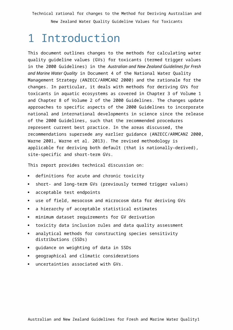
The reliability classifications to be applied to GVs derived using SSDs are listed in Table 4. In keeping with the discussions in Section 5, the minimum data requirements in Table 4 refer to single species laboratory-based testing, but these could be supplemented with data from microcosm, mesocosm or field studies where these meet the data quantity and quality requirements. This is especially appropriate for site-specific GV derivation. The hierarchy of preferred data types considered is: all chronic data > mixed chronic and converted acute data or, for organic chemicals only, combined chronic fresh and marine data > acute data converted to chronic data. The assignment of a reliability rating to the GVs is based on the data type, number of data points, and the adequacy of the fit (as ‘good’ or ‘poor’) of the SSD model to the data. As noted above, in the 2000 Guidelines, there were many instances where the GV was considered high reliability, but where the fit of the SSD model was obviously poor. A poor fit indicates a model that does not appear to be a good representation of the data points either at the low end of the SSD, or of the entire dataset.
Examples of good and poor data fits are shown in Figure 1. Poor fits can be the result of a poor fit of the Burr Type III or log-logistic distribution to the data points (Figure 1a), where the data appear to be poorly fitted to these distributions (for instance potentially bimodal) (Figure 1b), or where there is an inadequate spread of the data (Figure 1c). The occurrence of the same NOEC concentration for several test organisms (Figure 1c) arises due to the defined dilution/concentration series used for determining an NOEC value. The derivation and use of EC10 values would likely result in differing values for these organisms, especially if the determination followed the recommendation to include more measurements for concentrations at the low end of the concentration-response relationship.
Although the model fit and the associated GVs are independent of the plotting positions of the toxicity values in the SSD (see Section 9 for details), a visual check of the extent to which the model corresponds to the data is a worthwhile exercise for the reliability classification (notwithstanding the limitations associated with fitting such models to, typically, very few data). As the current GV derivation method does not weight the toxicity values in the SSD, all values in the dataset contribute equally to the model fit, and values at the lower end do not have a bigger influence on the model. Thus, any visual assessment of goodness-of-fit should take into account the whole of the distribution, not only the lower left end. Nevertheless, the GVs are estimated from the lower end of the distribution and, thus, a poor model fit in this region would be cause for concern.
Given the level of subjectivity in determining the fit of the SSD model, it may be preferable to have a panel of at least three relevant experts agree on the fit, especially where the decision is less clear. Moreover, for default GVs, the independent review process will provide a further assessment of the decision on the model fit. Ideally, site-specific GVs should also be independently reviewed, while further review would also be made by the relevant regulatory body in the event such GVs are submitted for a particular purpose. These review processes should ensure that the final decision on SSD model fit is appropriate and defensible.
Australian and New Zealand Guidelines for Fresh and Marine Water Quality 21

Technical Rationale for Changes to the Method for Deriving Australian and New Zealand Water Quality
Guideline Values for Toxicants
Figure 1 Examples of poor (a, b, c) and good (d, e) fits of data obtained using the revised Burrlioz 2.0 software (log-logistic fits were obtained for datasets of <8, and Burr Type III fits for ≥8)
The reliability scheme shown in Table 4 represents a technical evaluation of the level of confidence in a GV, which, when combined with other relevant knowledge (for instance information on toxicant use and environmental concentrations), can help determine: (i) the appropriateness of the GV, and (ii) priorities for future GV revisions. It is important to note that while the preferred GV derivation has a good fit to ≥8 15 data points, it is recognised that achieving such large datasets may not be possible in many instances, and that most derivations will use ≥8 data points. Bearing in mind that, in
Australian and New Zealand Guidelines for Fresh and Marine Water Quality 22
c d
e
ba

Technical Rationale for Changes to the Method for Deriving Australian and New Zealand Water Quality
Guideline Values for Toxicants
the 2000 Guidelines, five data points were sufficient for a high reliability GV, our re-evaluation recognises that this is rarely so, so these are now reclassified as moderate reliability at best, and low reliability if the fit is poor.
As noted by Warne et al. (2018), there are other factors that are not considered in the assessment of GV reliability that may affect the accuracy of the resulting GV. Two such factors are:
Toxicity datasets spanning 4 or more orders of magnitude. The GVs based on data with such a large range of values tend to be highly conservative and uncertain, especially at the 99% species protection level (PC99 level).
For persistent, bioaccumulative and toxic (PBT) chemicals, where there is a strong reliance on single-generation toxicity studies, it is important to note that GVs that are not based on multi-generation tests are unlikely to provide sufficient protection to aquatic ecosystems.
An SSD plot that spans 4 or more orders of magnitude (for instance Figure 1b) is indicative of differing modes of toxic action. This is seen for some bioaccumulating organic chemicals including 2,4-D, simazine and perfluorooctane sulfonate (PFOS) (King et al. 2017), as well as for aluminium in marine waters where toxicity is due both to dissolved and particulate forms (Golding et al. 2015). A consequence of the broad SSD plot is that extrapolation to a PC99 value has large errors and results in an extremely conservative value. This may be in part due to the Burr Type III distribution used to fit the curve, which requires further investigation. Bioaccumulating chemicals are particularly problematic because of the requirement for the use of a more conservative GV (PC99 rather than PC95) (ANZECC/ARMCANZ 2000). With bioaccumulating/biomagnifying compounds, the desirability of including multi-generational tests has been discussed by Warne et al. (2018).
Australian and New Zealand Guidelines for Fresh and Marine Water Quality 23

Technical Rationale for Changes to the Method for Deriving Australian and New Zealand Water Quality
Guideline Values for Toxicants
Table 4 Classification of the reliability of derived guideline values
SAMPLE SIZEa DATA TYPE ADEQUACY OF SAMPLE SIZE
ADEQUACY OF FIT IN SSD
RELIABILITY
Guideline values derived using a species sensitivity distribution
≥15
Chronicor combined chronic and converted chronic
PreferredGood Very high
Poor Moderate
8–14 GoodGood High
Poor Moderate
5–7 AdequateGood Moderate
Poor Low
≥15
Mixed chronic and converted acuteor mixed fresh chronic and marine chronic
PreferredGood Moderate
Poor Low
8–14 GoodGood Moderate
Poor Low
5–7 AdequateGood Moderate
Poor Low
≥15
Converted acute
Preferred Good Moderate
Poor Low
8–14 GoodGood Moderate
Poor Low
5–7 AdequateGood Low
Poor Very low
Guideline values derived using an assessment factor
<5 Chronic, mixed chronic and acute, or converted acute Inadequate Not applicable Unknown
a For the SSD method, the sample size is assumed to comprise data from at least 4 taxonomic groups.
8.2 Selection rules for toxicity data to be used in species sensitivity distributions
The rules for manipulation of toxicity data to obtain a single value for each species have been changed from the 2000 Guidelines (ANZECC/ARMCANZ 2000, Warne 2001) and are expressed below.
For each chemical, the toxicity data that have passed the data quality assurance process should first be sorted by species, then endpoint and finally by duration of exposure. For each combination of species and endpoint, the longest exposure duration is selected, unless the toxicity estimate from a shorter duration is lower, then the lower value should be chosen. If there are multiple values for the accepted duration then calculate the geometric mean. Select the lowest resulting value for each combination of species and endpoint. The toxicity value for the most sensitive endpoint for each species should be adopted as the sensitivity value for that species. An example of the application of these rules to a dataset is presented in Table 5.
Australian and New Zealand Guidelines for Fresh and Marine Water Quality 24

Technical Rationale for Changes to the Method for Deriving Australian and New Zealand Water Quality
Guideline Values for Toxicants
Table 5 Example of the application of data selection rules for a species
SPECIES ENDPOINT DURATION (h) EC10 (mg/L)
VALUE FOR EACH COMBINATION OF
SPECIES, ENDPOINT AND DURATION
(µg/L)
LOWEST VALUE FOR
EACH COMBINATION
OF SPECIES AND
ENDPOINT (µg/L)
LOWEST VALUE
FOR SPECIES
(µg/L)
Ceriodaphnia cf. dubia
Growth 168 7 7 7
0.19
C. cf. dubia Immobilisationa 168 10
5.3 5.3C. cf. dubia Immobilisation 168 5
C. cf. dubia Immobilisation 168 3
C. cf. dubia Reproduction 240 1.3
1.3
0.19
C. cf. dubia Reproduction 240 2.0
C. cf. dubia Reproduction 240 0.9
C. cf. dubia Reproduction 480 0.2
0.19C. cf. dubia Reproduction 480 0.15
C. cf. dubia Reproduction 480 0.24
a Immobilisation for cladocerans is strictly not mortality but is treated as an equivalent endpoint for these species, as individuals that are unable to move in response to an external stimulus are unlikely to be able to filter feed and/or avoid predators. Mortality in cladocerans is defined as the heart not beating.
Where water quality may have significantly varied across the tests for some reason (for instance in studies specifically designed to assess the effects of physicochemical variables, such as pH, hardness or dissolved organic carbon, on toxicity), then best professional judgement will need to be applied as to whether the geometric mean or the lowest toxicity value from across the tests should be used for the GV derivation. Where tests for individual species have demonstrated a significant dependence of toxicity on a physicochemical variable, then the toxicity data that correspond to the most toxic set of conditions should be used for GV derivation. Justification for all decisions relating to these issues needs to be provided. Where the measured value of an important physicochemical variable (that is one that affects the toxicity of the contaminant in question) in the toxicity test dilution water is well beyond the typical range of that variable in Australia and New Zealand (see Section 8 and Table 3), then best professional judgement should be applied to determine whether or not the toxicity value associated with that test should be included in the dataset.
It is worth noting that the European Commission (2011) does not use geometric means but rather defers to best professional judgement. However, the geometric mean is used by Canada (CCME 2007), the USA (Stephan et al. 1985) and, previously, Australia and New Zealand in the 2000 Guidelines (ANZECC/ARMCANZ 2000).
8.3 Dealing with toxicity modifying factorsIn deriving some GVs, toxicity is known to be dependent on other physical and chemical factors. This is particularly so with metals, with a dependence on hardness, pH, alkalinity and/or dissolved organic carbon. Contaminants such as ammonia, cyanide, phenols have a pH dependence (ANZECC/ARMCANZ 2000). From a theoretical point of view, the toxicity of many, if not most organic
Australian and New Zealand Guidelines for Fresh and Marine Water Quality 25

Technical Rationale for Changes to the Method for Deriving Australian and New Zealand Water Quality
Guideline Values for Toxicants
chemicals, is likely to be affected by a range of properties including pH, dissolved organic and total organic carbon content and the concentration of total suspended solids. However, to date, quantitative relationships between toxicity and these factors that could be used to calculate site-specific GVs are not available for organic chemicals.
In the 2000 Guidelines, derivations for metals were based as much as possible on data for a fixed pH, and hardness, with hardness corrections using accepted algorithms being used for cadmium, chromium, copper, lead, nickel and zinc (ANZECC/ARMCANZ 2000, Markich et al. 2001). However, much of the work on which the algorithm for copper was derived ‘confounded the effects of true water hardness (Ca/Mg), with alkalinity (carbonate concentration) and/or pH’ (Markich et al. 2006). Furthermore, the algorithms were largely derived from North American acute fish toxicity data and their relevance to chronic data for other species is unknown; they have not been verified for freshwater plants (algae and macrophytes) due to a lack of data. More recent work that examined the effect of true water hardness generally found that it did not affect copper toxicity to a variety of freshwater organisms including bacteria, a unicellular green alga, a macrophyte, a hydra, a bivalve, crustaceans and fish (Lauren and McDonald 1986, Pynnӧnen 1995, Reithmuller et al. 2000, Grosell and Wood 2002, De Schamphelaere and Janssen 2004, Hyne et al. 2005, Markich et al. 2005, Markich et al. 2006), while a few have found it had a significant but small effect (Erickson et al. 1996, Perschbacher and Wurts 1999, Heijerick et al. 2005). Therefore, for the revised GV derivation method, it is recommended that the copper GV hardness correction algorithm is not used to tailor the GV to local water hardness.
Metal speciation is specifically considered in the assessment hierarchy against GVs for laboratory-based testing. The bioavailable fraction can be measured, modelled or determined by toxicity testing and the bioavailable concentration compared to the GV. This approach is promoted in the 2000 Guidelines and continues to be adopted.
An alternative methodology is based on the biotic ligand model (BLM). The biotic ligand is a key binding site in an organism at which there is competition for binding between metals and other cationic components of the water, protons and base cations (Na+, Mg2+, K+, Ca2+), while there is competition for the metal between the biotic ligand and dissolved organic carbon (DOC). Binding constants are derived for the reactions of these species, as well as the metal of interest, with the biotic ligand. The derivation procedures are complex and a suite of BLM binding equations must be developed for acute and chronic toxicity data for key species groups (that is fish, invertebrates and algae). The multiple BLM equations can then be combined for application to deriving site-specific water quality GVs that incorporate conditions such as pH, DOC and hardness. Early BLMs examined acute toxicity, however, chronic BLMs are required for GV derivation.
To date, BLMs have been derived for use in toxicity prediction for copper (for example Santore et al. 2001, De Schamphelaere et al. 2002, De Schamphelaere and Janssen 2004, USEPA 2007), nickel (Keithly et al. 2004, Hoang et al. 2004), silver (Paquin et al. 1999), zinc (Heijerick et al. 2002a, b) and manganese (Peters et al. 2011). More recently, representatives of Australian regulatory agencies, academics and consultants have been working collaboratively with the Nickel Producers Environmental Research Association (NiPERA) and WCA Environment Limited (England) to determine the validity of the nickel BLM, which was initially developed for Europe, to suit Australian conditions and biota (Peters et al. 2013, 2018).
Australian and New Zealand Guidelines for Fresh and Marine Water Quality 26

Technical Rationale for Changes to the Method for Deriving Australian and New Zealand Water Quality
Guideline Values for Toxicants
The BLM calculations can be used to adjust toxicity values to a standardised, ‘normalised’ set of water quality conditions prior to deriving water quality GVs, and to make adjustments to generic GVs to suit site-specific water quality conditions. Slightly different models have been used in USA (USEPA 2007) and Europe (Bass et al. 2008), incorporating different predictive equations. The complexity of the BLMs, requiring the application of differing species-specific BLM binding coefficients, and calibrations over a wide range of water quality modifiers (that is DOC, Ca, Mg, pH) requires an intensive calibration effort and multi-parameter mathematical calculations for implementation. A simplified and more user-friendly BLM, has been developed by Bio-Met (2013). Hickey et al. (2017) reviewed the BLM application to copper and zinc GVs in freshwater. They noted that modifiers may result in different response relationships for different taxonomic groups, dependent also on the duration of test exposures (acute or chronic), adding significant complexity to normalising toxicity data to a standard water quality condition. The alternatives to application of a BLM modifier approach are to censor the toxicity data in relation to the modifiers in order to bound variability, which might be associated with that parameter, or exclude data where there is a high likelihood that strong effects will be occurring (for instance DOC). The uncertainty of the BLM predictions for copper does not favour implementation for GV derivation at this time. Rather, the database for GV derivation should be based on bounded data for key water quality modifiers so as to limit variability attributable to water quality modifiers, for example, only use data in the pH range 6.0 to 9.0.
Another approach is to develop relationships between toxicity and modifying factors, as has been done with the revised Australian sediment quality guidelines (Simpson et al. 2010) and the Australian Ecological Investigation Levels for contaminated sites (NEPC 2013). An example of this is the work by van Dam et al. (2012) on the influence of dissolved organic carbon on uranium toxicity. The use of multiple linear regressions (MLRs) is being adopted by Environment Canada in their revised draft water quality GV for zinc (Environment Canada 2016). Two- or three-parameter MLRs can be derived, either as empirical models to fit existing datasets or as simplified versions of existing models. Using this approach, the Canadian Guidelines generate a lookup matrix table for the water quality modifiers. Similar to the BLM approach, toxicity data from a single species can be used to develop relationships, or data for multiple species can be pooled to select the best MLR, provided that water chemistry effects on toxicity are similar across species. The MLR approach may assist the transition from simple algorithm approaches to more complex BLM approaches for metal water quality GV derivations.
Australian and New Zealand Guidelines for Fresh and Marine Water Quality 27

Technical Rationale for Changes to the Method for Deriving Australian and New Zealand Water Quality
Guideline Values for Toxicants
9 Analytical methods for deriving species sensitivity distributions
An SSD is a probabilistic model of the distribution of the toxicity of particular contaminants to a defined range of species representing a specified number of taxonomic groups. It is used to determine a contaminant concentration that is theoretically protective of a given percentage (x) of species (that is the protective concentration to x% of species, PCx), often expressed in risk assessments as the concentration that is hazardous to a given percentage (y) of species (that is HCy, where y=100-x).
In Australia and New Zealand, it has been agreed that toxicant GVs should be based on the following levels of species protection:
High conservation value ecosystems: 99% species protection (PC99; HC1)
Slightly-to-moderately disturbed ecosystems: 95% species protection (PC95; HC5)
Highly disturbed ecosystems: 90% or 80% species protection (PC90; HC10 or PC80; HC20).
The PC99 is often an extrapolated value (outside the range of the toxicity data) and in these cases should be interpreted cautiously.
A number of statistical models are used for SSDs that include both parametric and non-parametric methods (for example Wheeler et al. 2002, Hickey and Craig 2012). Commonly used parametric methods that have been used include the following distributions: logistic, log-logistic, log-normal. Burr Type III, Gompertz, and log-triangular. Given the small datasets often used to derive GVs, it has generally been found that any reasonable candidate distribution will not be rejected by a statistical test of goodness-of-fit due to low statistical power. However, there are a number of reasons for rejecting the log-triangular distribution (Warne 1998).
In Australia and New Zealand, the Burr Type III distribution was adopted in 2000 as the preferred distribution to be fitted to the toxicity data. This was incorporated into the BurrliOZ software (Campbell et al. 2000). This software has generally performed well, giving acceptable data fits, although in some cases there were problems with small datasets. There are statistical reasons why the three-parameter Burr Type III distribution is inappropriate to deal with small datasets (5–7 species). Although not solving all of the problems associated with this, it is preferable to use a simpler model such as the two-parameter log-logistic distribution for small datasets. Adopting this approach is likely to resolve some of the existing problems with small dataset SSDs. The revised SSD analytical approach described here has been incorporated into an updated version of the Burrlioz software for deriving GVs (https://research.csiro.au/software/burrlioz/). This software will provide a 95% confidence interval around the selected PCx values. This is designed to provide a measure of statistical confidence around the PC values, however, it is important to note that it is not intended that the lower range of the confidence interval be used as the GV.
The log-logistic distribution has a long and established role in ecotoxicology (for example Aldenberg and Slob 1993). Even though there is no biological/ecological/environmental/ecotoxicological basis
Australian and New Zealand Guidelines for Fresh and Marine Water Quality 28

Technical Rationale for Changes to the Method for Deriving Australian and New Zealand Water Quality
Guideline Values for Toxicants
for choosing one statistical distribution over another, there is at least a precedent for defaulting to the log-logistic distribution, and it does perform reasonably well under a wide variety of conditions. It cannot return negative PCx values because it is constrained to lie on the interval (0 to infinity) and, if we accept that fitting any distribution with such small samples is not best statistical practice, then we should at least be careful not to overfit, that is, using more parameters that can be justified by the sample.
The log-logistic or Burr Type III distribution is fitted, and the GVs are estimated, using a maximum likelihood approach, not a regression fitting approach. As such, the fitted model, and its associated GVs, is independent of the exact plotting positions of the toxicity values. Thus, although different SSD-fitting software applications may use different plotting position equations that typically plot the points in slightly different positions (with this difference being more pronounced for small sample sizes), the plotting position equation will have no effect on the estimated GVs from the model.
There is also the option to apply non-parametric approaches to SSD fitting. A bootstrap regression method has been described by Grist et al. (2002). Bayesian methods have been described by Fox (2009) and Hayashi and Kashiwagi (2013). Such approaches should be explored in future revisions of toxicant GV derivation methods.
Of importance is the understanding of the precision afforded by the PCx estimates. The GVs reported in the 2000 Guidelines are the median of the distribution of PC95 estimates. Use of a lower 95% confidence interval (for instance PC95, 95) is inappropriate, particularly for small datasets, given the lack of precision at the tail of the confidence limit distribution coupled with that on the tail of the SSD distribution. Most jurisdictions recommend the use of a PC95, 50. To simplify notation and comprehension by users, the PCx, 50 values have been simplified to PCx values (where x values are commonly 99, 95, 90 or 80).
Australian and New Zealand Guidelines for Fresh and Marine Water Quality 29

Technical Rationale for Changes to the Method for Deriving Australian and New Zealand Water Quality
Guideline Values for Toxicants
10 Guidance on weighting of data in species sensitivity distributions
The method of deriving toxicant GVs using SSDs requires data for at least five species that belong to at least four taxonomic groups. Where there is more than one data point for the same exposure duration and species, a single value is used to represent each species (Warne (2001) and also see Section 8.1). In determining a single sensitivity value for each species, equal importance (weighting) is given to each species in calculating the SSD and the resulting GV. The way in which data from different species are dealt with in SSDs has received criticisms from several authors. Forbes and co-workers (Forbes and Forbes 1993, Forbes and Calow 2002) made the point that only a fraction of the species going into the SSD determines the effects threshold. With all species being weighted equally, the loss of any species is considered to be of equal importance to the ecosystem, and keystone, foundation or other important species are assumed to be randomly distributed in the SSD (although for site-specific GV derivation, this may not be the case). For example, they suggested that while an ecologically realistic distribution of species by trophic level was 64% primary producers, 26% herbivores (invertebrates) and 10% carnivores (fish), a mean ratio from typical SSDs for different chemicals was found to be 28, 35 and 38% respectively. Thus, fish were over-represented and primary producers under-represented. Re-sampling the species sensitivity database to reflect a more environmentally realistic distribution of trophic levels yielded a PC95 value 3.4 times lower for cadmium than when the data were given equal weighting (Forbes and Calow 2002). By contrast, the PC95 value for linear alkylbenzene sulfonate (LAS) based on an environmentally realistic distribution of trophic levels was 3.2 times higher than the PC95 when the same data were given an equal weighting (Forbes and Calow 2002). One of the underlying assumptions of all SSD methods is that the species used in the SSD should be a random selection of the species in the ecosystem; however, our selection is typically biased by the availability of toxicity tests, which may be exaggerated further for small datasets. Targeting keystone taxa in the SSD and derived GV is highly recommended if tests are available.
Duboudin et al. (2004) followed this up by questioning: (i) how to deal with the various test results that exist for the same species, and (ii) how to account for the variability in the available data for a particular taxonomic class (for example algae, invertebrates, vertebrates). They compared SSDs that used: (i) the literature ratio of data in these classes (that is unweighted data), (ii) one that weighted these classes equally (using the geometric mean of multiple species data, that is the Australian and New Zealand approach); and (iii) one using the environmentally realistic ratio for these three species classes used by Forbes and Calow (2002), and observed up to an order of magnitude difference in GVs between the three data treatments. The choice of data (intra-species variation and proportions between taxonomic groups) was found to have more effect on the value of the PC95 than the statistical method used to construct the distribution (Duboudin et al. 2004). They recommended that rather than using the geometric mean of multiple data for the same species, to weight data to retain intra-species variation while giving each species the same weight within the SSD. This uses the entire set of data, so as not to favour one species over the others, however, when the number of data points is low, the PC95 can be dominated by a few large weighted data points. This highlights the
Australian and New Zealand Guidelines for Fresh and Marine Water Quality 30

Technical Rationale for Changes to the Method for Deriving Australian and New Zealand Water Quality
Guideline Values for Toxicants
desirability of having large datasets that cover a range of species and taxonomic groups as discussed in Section 8.
Rather than using SSDs for all aquatic organisms, Brix et al. (2001) applied SSDs to individual taxonomic groups, for estimating the risks of dissolved copper to specific taxonomic groups. This is possible because there is quite a large dataset available for copper. The results were compared with a site-specific food web to determine whether key food web components are potentially at risk and whether the overall aquatic community is at risk in relation to ecosystem function. In this example, substantial risk was observed for a zooplankton–planktivorous fish–piscivorous fish food web, because cladocerans were shown to be at greatest risk. While such an approach is ideal, data limitations make it impractical for most applications and not appropriate for deriving default (that is national level) GVs.
Grist et al. (2006) discussed ways in which expert judgement can be incorporated into SSDs using a Bayesian approach that may be applicable to weighting approaches to data.
For toxicant GVs, where possible, input data should cover important species, but apply weighting based on natural abundance or other such factors and the validity of doing this requires more research before it can be recommended. The major limitation is usually one of insufficient data. There is generally insufficient information on which to make decisions on how to weight the data, so the current system of giving each species equal weighting is to be retained.
Implicit in the statistical distribution-fitting exercise is the untested, but surely false assumption that the data represents a truly random sample from the population of all species. How we accommodate our ‘selection bias’ in SSD-fitting is another unresolved issue that requires further research. Weighting might be usefully considered for site-specific assessments and the calculation of site-specific GVs where the information needed to determine the weightings may be available, but as with all deviations from the national approach, the method must be transparent and scientifically valid.
Australian and New Zealand Guidelines for Fresh and Marine Water Quality 31

Technical Rationale for Changes to the Method for Deriving Australian and New Zealand Water Quality
Guideline Values for Toxicants
11 Geographical/climate-specific considerations for species/data inclusion
Guideline values for Australia and New Zealand are typically derived from North American and European data because of the limited local database, particularly of chronic toxicity data. Australia, however, encompasses environments ranging from tropical to polar and whether there is a need for different GVs for each environment or climate is an issue of concern. There have been several attempts to compare sensitivities of temperate and tropical species (Leung et al. 2001, Wheeler et al. 2002, Maltby et al. 2005, Kwok et al. 2007, Daam and van den Brink 2010), and temperate, tropical and polar species (Chapman and Riddle 2005), using species sensitivity distributions. These have largely been confined to acute rather than chronic endpoints. Overall, the findings suggest that any differences in acute toxicity are dependent on both the chemical and the species being compared.
For freshwater species, Kwok et al. (2007) generalised that for most metals tropical species were less sensitive (for zinc the reverse was true), while for ammonia, phenol and some pesticides, tropical species were more sensitive (based on ratios of temperate to tropical EC10 values). Based on applying various SSD methods to the ratios of temperate to tropical EC10 data, they recommended that temperate GVs be divided by 10 if being used for tropical and sub-tropical regions. Based on the latest most comprehensive data for marine species, PC90 temperate/tropical ratios of 0.5, 1.7, 0.8, 1.5, and 1.6 for cadmium, copper, zinc, pentachlorophenol and phenol, respectively, were reported, while the ratio for tributyltin was 8.5 (Wang et al. 2011). The variable data serve to point out that there is no consistent relationship between tropical and temperate GVs, largely because the species sample sizes are so small.
Comparative testing of species must involve conditions of optimum health, where the organisms are unstressed by temperature. There are a number of factors that might affect species response at different temperatures. Rates of metabolism, detoxification and elimination typically increase with temperature (Daam and van den Brink 2010). Studies of fish species reported sensitivities to DDT (Dyer et al. 1997) in the order cold water > temperate > tropical species, but for many other pesticides there were no significant differences (Dyer et al. 1997, Maltby et al. 2005). A comparison of the acute toxicity of oil components to polar and temperate marine species found that except for naphthalene, toxicities (as HC50s) did not differ significantly (de Hoop et al. 2011). Even the HC5 values for naphthalene were comparable. There have so far been no comparisons based on chronic endpoints.
It was noted that USA and Canadian regulators had exclusion rules that did not accept data from other geographic regions, although the Canadian protocol now accepts data from non-resident species, as long as they can be considered as appropriate surrogates of local species (CCME 2007). Excluding international data would have unacceptable consequences for Australian and New Zealand GV derivations. Therefore, it was decided to not derive geographic or climate-specific GVs in the 2000 Guidelines or in the current revision. Where such GVs are required, particularly for tropical and
Australian and New Zealand Guidelines for Fresh and Marine Water Quality 32

Technical Rationale for Changes to the Method for Deriving Australian and New Zealand Water Quality
Guideline Values for Toxicants
Antarctic ecosystems, it is recommended that these should be derived using region-specific (or climate-specific) data.
The same data requirements that apply to the default GVs would apply to these regional or site-specific GVs. In general, tropical and polar species are under-represented in the Australian and New Zealand species datasets, and obtaining new data for these climatic regions is encouraged.
An example of site-specific, or regional, GVs in this category are those derived to protect Australia’s Great Barrier Reef (GBRMPA 2010). In particular, GVs were derived for pesticides not covered by the 2000 Guidelines, mostly with a desired level of protection of 99%. Consideration was given to the effects of the sub-lethal endpoint of suppression of photosynthesis of corals on calculated GVs, however, at this stage, GVs were set without the sub-lethal responses included (refer to Section 4).
Particular problems are experienced in deriving GVs for polar regions where very long exposure durations are required to reach mortality in toxicity testing, or if this is to be reached within a reasonable test duration of 2–3 weeks, often require unrealistically high concentrations of contaminants. Here, data based on behavioural endpoints might constitute a large proportion of the toxicity database, and the links to ecological relevance are not readily demonstrated. In the absence of sufficient other data, these would be admissible for region-specific guideline derivation, as the only means by which GVs could be realistically achieved.
On a related area of data availability, there are generally more freshwater toxicity data than data for marine species, and it has been advocated that in such cases, freshwater data could be included in the marine database. Leung et al. (2001) showed that for many metals, the agreement was remarkably good between SSDs based only on marine or only on freshwater data. Where the marine dataset is small (less than eight species), the addition of data for freshwater species may be considered to improve the reliability of the GV derivation (see Section 7). An alternative approach, recommended in the 2000 Guidelines, would be to adopt the freshwater GV as a low reliability marine GV. However, using either of the above approaches would, in the case of metals, require consideration of speciation issues. It is therefore not recommended that fresh and marine ecotoxicity data be combined for metals in order to derive default GVs.
Australian and New Zealand Guidelines for Fresh and Marine Water Quality 33
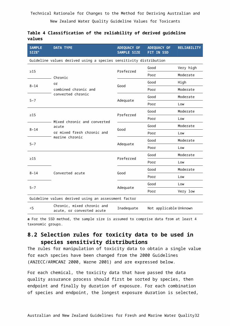
Technical Rationale for Changes to the Method for Deriving Australian and New Zealand Water Quality
Guideline Values for Toxicants
12 Uncertainties associated with guideline values
In addition to those discussed above, there are a number of other sources of uncertainty in GV derivations that are often overlooked in defining the precision of the derived value. These arise either from uncertainties associated with the toxicity test procedure, or from uncertainties in the model used to derive the GVs.
The variability in toxicity testing, both intra- and inter-laboratory, can come from many sources, including differing sensitivities of the test organism (within and between laboratories), differences in response of individuals of a test species; differing laboratory procedures and practices, analytical errors associated with measuring low toxicant concentrations, losses on container surfaces, analytical errors, errors in measuring the organism response, errors in replication, changes in chemical form of the toxicant, and choice of dilution series.
A comprehensive study by Moore et al. (2000), found intra-laboratory coefficients of variation (CVs) on EC25 values for Ceriodaphnia dubia exposed to a sodium chloride reference toxicant, of between 16 and 56% irrespective of whether the endpoint was mortality or reproduction. For the fish Menidia beryllina exposed to a copper reference toxicant, CVs ranged from 24–61% for mortality and 24–122% for biomass. Inter-laboratory CVs were 13–17% for the Ceriodaphnia and 66–177% for the Menidia. Such variability is consistent with other published studies (for instance Thellen et al. 1989, Warren-Hicks et al. 2000). Derived NOEC values that make up the bulk of our existing toxicity database are critically dependent on the dilution series adopted. It is not meaningful to talk of errors or uncertainties in the NOEC since it is simply a numeric label derived from multiple-comparison testing procedures (Fox et al. 2012).
To minimise variability, good quality assurance and quality control of toxicity testing is required including: (i) analysis of all toxicant concentrations used in the toxicity test at the beginning and end of the test; (ii) use of a reference toxicant; (iii) appropriate control and measurement of experimental conditions, for example, temperature, pH; (iv) quality control of the test containers, for example water changes, organism feeding; and (v) a reproducible control response.
The variability associated with the use of ECx values will reduce by increasing the number of test concentrations in the concentration-response curve, particularly at the lower end.
Toxicity data with their own variability are assembled into a model to calculate an appropriate GV. Here there are uncertainties associated with the chosen models, including model parameterisation, different methods of estimation and stochastic variation. The revised Burrlioz 2.0 software allows plotting of the 95% confidence intervals around the PCx value reflecting the goodness of fit of the distribution to the species sensitivity data (but not taking into account uncertainty in the toxicity estimates themselves). The wide range of these confidence intervals will come as a surprise to many. Their magnitude is highly dependent on the size of the datasets, the nature of the statistical model used, and assumptions about the random error term.
Australian and New Zealand Guidelines for Fresh and Marine Water Quality 34

Technical Rationale for Changes to the Method for Deriving Australian and New Zealand Water Quality
Guideline Values for Toxicants
It is important to understand the sensitivity of the derived GVs to the data values. For example, using the available 43-point database for chromium (VI) in marine waters (ANZECC/ARMCANZ 2000), it was shown that the PC95 could vary by more than a factor of 2 by choosing the lowest data rather than the geometric mean of replicates (G. Batley, pers. obs.). Adding points to the low concentration end of the dataset had the expected effect of lowering the GV, while adding data points to the high concentration end significantly increased the GV in this case, although in other cases a lowering of the GV has been observed. Our choice of test organisms is often biased to those cultured in the laboratory, but is this an acceptable bias? While these are usually representative of naturally occurring species, the relevance of laboratory-based tests to field conditions remains an issue.
It is important to recognise that the EC10, which we are promoting as a more reliable endpoint than the NOEC, represents a 10% chronic sub-lethal effect on the test organism (with its associated confidence limits). We are then using these values to derive a PC95. The question might be raised as to whether 10% chronic sub-lethal toxicity to 5% of species is ecologically acceptable. This is primarily a question of population viability. Most populations can withstand a 10% decrease in productivity (fisheries management and most other ecosystem resource use is based on this assumption). The assumption of the GV derivation method is that the test species are adequately representative of the sensitivities of other ecosystem constituents such that, at most, 5% of taxa in the ecosystem might suffer some population viability impairment. If that assumption holds, it is a more conservative position than that of most resource management decisions, and implies that most aspects of ecosystem function will be minimally impaired, if at all.
Note that the uncertainties in estimating a 99% species protection (PC99) GV from an SSD are larger than that for the PC95 because there is less confidence in the SSD model fit at the extremes of the distribution compared to the middle. This is especially so for small datasets. Professional judgement should be applied in assessing the extent to which the extrapolation of the SSD to a PC99 value generates an acceptable number. Considerations might include whether the GV concentration is consistent with accepted background concentrations, and the lowest toxicity estimates. Similarly, there are generally greater uncertainties associated with EC5 values than EC10 values if they are determined using the same experimental design.
These issues are being raised in order to encourage awareness among users of the uncertainties associated with GVs. To this end, the combined uncertainties should be recognised in how GVs are reported. These should be refined to no more than two significant figures, taking into account the standard rounding-off rules, for example, a GV of 237 µg/L should be reported as 240 µg/L.
It is important to recognise that uncertainties in GVs become less important in the context of the recommended use of multiple lines of evidence for evaluating toxicant impacts. Thus, toxicant concentrations near a low or moderate reliability GV might indicate concerns if toxicity can be demonstrated, if there is significant bioaccumulation, and there are effects on ecosystem abundance and diversity. If there is counter-evidence, any observed toxicity might be attributed to another unidentified source. Further guidance on how GVs should be used as part of a weight of evidence process are provided by ANZG (2018; http://www.waterquality.gov.au/anz-guidelines/resources/key-concepts/weight-of-evidence).
Australian and New Zealand Guidelines for Fresh and Marine Water Quality 35

Technical Rationale for Changes to the Method for Deriving Australian and New Zealand Water Quality
Guideline Values for Toxicants
GlossaryTerm Definition
ACR Acute to chronic ratio
Acute toxicity An adverse sub-lethal effect that occurs as a result of a short exposure period to a chemical relative to the organism’s life span
Alga Chlorophyll-bearing plants, most of which are aquatic. These can be microscopic in size and single celled (such as microalgae) or multicellular macroalgae (such as seaweeds)
Amphipod Small crustaceans (typically <10 mm) found in most aquatic environments
ANZECC Australian and New Zealand Environment and Conservation Council
Aquatic ecosystem Any water environment in which plants and animals interact with the chemical and physical features of the environment
ARMCANZ Agriculture and Resource Management Council of Australia and New Zealand
Bayesian Involving statistical methods that assign probabilities or distributions to events or parameters based on experience or best guesses before experimentation and data collection and that apply Bayes' theorem to revise the probabilities and distributions after obtaining experimental data
BEC10 Bounded effect concentration in a toxicity test that is the highest tested concentration that has an upper 95% confidence interval that causes less than a 10% effect
Benthic Organisms living in or on the sediments of aquatic habitats
Bioaccumulation A general term describing a process by which chemical substances are accumulated by aquatic organisms from water directly and/or through consumption of food containing the chemicals
Bioavailable Able to be taken up by organisms
Bivalve A mollusc with a shell in two parts, hinged together
Biotic ligand model (BLM) Models that consider the effect of water parameters, including water hardness, pH and dissolved organic carbon, to model the bioavailability of metals. The ligand is the gill surface
Bootstrapping A statistical re-sampling technique typically used to estimate functions of statistics (for example standard errors) when analytical expressions are unavailable
BurrliOZ and Burrlioz A species sensitivity distribution software package developed and used in the 2000 Guidelines to derive guideline values (previously termed trigger values) to protect aquatic ecosystems. BurrliOZ denotes the original version of the software, while Burrlioz and Burrlioz 2.0 denote the second, improved version of the software
Burr Type III A flexible family of parametric distributions for non-negative data
CCME Canadian Council of Ministers of the Environment
Chronic toxicity An adverse effect that occurs as the result of exposure to a chemical for a substantial portion of the organism’s life span or a sub-lethal adverse effect on a sensitive early life stage
Community An assemblage of organisms characterised by a distinctive combination of species occupying a common environment and interacting with one another.
Community composition All the types of taxa present in a community
Concentration The quantifiable amount of a substance in water, biota, soil or sediment
Contaminants Biological or chemical substances or entities, not normally present in a system, capable of producing an adverse effect in a biological system, seriously injuring structure or function
Australian and New Zealand Guidelines for Fresh and Marine Water Quality 36

Technical Rationale for Changes to the Method for Deriving Australian and New Zealand Water Quality
Guideline Values for Toxicants
Term Definition
Control Part of an experimental procedure that is ideally exactly like the treated part except that it is not subject to the test conditions. It is used as a standard of comparison, to check that the outcome of the experiment is a reflection of the test conditions and not of some unknown general factor
Copepod A small crustacean found in marine and freshwater habitats; many are planktonic (living within the water column), but more are benthic (living on or in the sediments)
Coefficient of variation (CV) The ratio of the standard deviation and the mean
Detection limit The concentration of a substance that, when processed through the complete analytical method, produces a signal that has a 99% probability of being different from the blank
DO Dissolved oxygen
DOC Dissolved organic carbon
Ecotoxicology The science dealing with the adverse effects of chemicals, physical agents and natural products on populations and communities of living organisms
EC50 The toxicant concentration that is expected to cause one or more specified effects in 50% of a group of organisms or a 50% effect under specified conditions
ECx The toxicant concentration that is expected to cause one or more specified effects in x% of a group of organisms or x% effect under specified conditions
Gompertz A probability distribution that has been used to model species sensitivity distributions
Guideline value (GV) A concentration of a toxicant that if exceeded, might potentially impair water quality and thereby trigger an investigation or initiate a management response
Hazardous concentration (HC) Hazardous concentration, usually to a given percentage of species, for example HC5 is the concentration hazardous to 5% of species
IC50 A toxicant concentration that would cause a 50% reduction in a non-quantal measurement such as fecundity or growth
Indicator Measurement parameter or combination of parameters that can be used to assess the quality of water
Invertebrate An animal lacking a notochord or backbone
LC50 The toxicant concentration that is expected to be lethal to 50% of a group of organisms under specified conditions
Level of protection The acceptable level of change from a defined reference condition
LOEC Lowest-observable-effect concentration; the lowest tested concentration of a material (toxicant) that corresponds to a statistically significant difference compared to control organisms
MATC Maximum allowable toxicant concentration: the geometric mean of the lowest exposure concentration that causes a statistically significant adverse effect (LOEC) and the highest exposure concentration where no statistically significant effect is observed (NOEC) in a chronic test
Measurement parameter Any parameter or variable that is measured to find something out about an ecosystem
Mesocosm Large enclosures designed to mimic field exposure conditions, taking the form of larger tanks, enclosures or artificial channels to mimic streams, often, but not necessarily, located in or near water bodies
Microcosm Laboratory-based bench-scale artificial ecosystems
Multiple linear regression (MLR) Regression equations where the y parameter is modelled using two or more xparameters
Australian and New Zealand Guidelines for Fresh and Marine Water Quality 37

Technical Rationale for Changes to the Method for Deriving Australian and New Zealand Water Quality
Guideline Values for Toxicants
Term Definition
Multi-generation toxicity test A toxicity test that exposes more than one generation of a test organism sequentially to the test chemical. The duration of multi-generation tests depends on the generation time of the test organism. For example, a typical 72-hour test for a microalga is strictly speaking a multi-generation test. However, a multi-generation test on a fish species could take months to years. Typically a multi-generation test will be of shorter duration than the average lifespan of the test organism. Multi-generation toxicity tests can only generate chronic toxicity data.
NOEC No-observable-effect concentration; the highest tested concentration of a material (toxicant) at which the measured response is statistically indistinguishable from the control response.
NWQMS National Water Quality Management Strategy
Organism Any living animal or plant
Persistent, bioaccumulative and toxic substances (PBT)
Substances that persist in the environment, bioaccumulate in organisms and cause toxic effects to humans or organisms from long-term exposure. The exact definitions vary in different jurisdictions
Protective concentration (PC) Protective concentration: PC95 is the concentration protecting 95% of species
Pesticide Substance or mixture of substances used to kill unwanted species of plants or animals
pH The intensity of the acidic or basic character of a solution, defined as the negative logarithm of the hydrogen ion concentration of a solution
Phylum A taxonomic rank below kingdom and above class
Quality assurance (QA) The implementation of checks on the success of quality control (for instance replicate samples, analysis of samples of known concentration)
Quality control (QC) The implementation of procedures to maximise the integrity of monitoring data (for instance cleaning procedures, contamination avoidance, sample preservation methods)
Redox Simultaneous (chemical) reduction and oxidation; reduction is the transfer of electrons to an atom or molecule, whereas oxidation is the removal of electrons from an atom or molecule
Reference toxicant A reference chemical (toxicant) used in a toxicity tests to assess the sensitivity of a test organism and to demonstrate the repeatability of a test and the laboratory's ability to perform the test consistently
Reference condition An environmental quality or condition that is defined from as many similar systems as possible (including historical data) and used as a benchmark for determining the environmental quality or condition to be achieved and/or maintained in a particular system of equivalent type
Risk Typically defined by the joint interaction of both the likelihood and consequence of an event having a negative or adverse impact. Estimates of risk may be expressed in absolute or relative terms. Absolute risk is the excess risk due to exposure. Relative risk is the ratio of the risk in the exposed population to the risk in the unexposed population
Salinity The presence of soluble salts in water or soils
Sediment Unconsolidated mineral and organic particulate material that has settled to the bottom of aquatic environments
Single-generation toxicity test A toxicity test that exposes a single generation of the test organism to the test chemical. Single-generation toxicity tests can generate either acute or chronic toxicity data, depending on the duration of the exposure (refer to acute and chronic toxicity)
Speciation Measurement of different chemical forms or species of an element in a solution or solid
Species A group of organisms that resemble each other to a greater degree than members
Australian and New Zealand Guidelines for Fresh and Marine Water Quality 38

Technical Rationale for Changes to the Method for Deriving Australian and New Zealand Water Quality
Guideline Values for Toxicants
Term Definition
of other groups and that form a reproductively isolated group that will not normally breed with members of another group. (Chemical species are differing compounds of an element)
Statistical power The ability of a statistical test to detect an effect given that the effect actually exists
Stressors The physical, chemical or biological factors that can cause an adverse effect on an aquatic ecosystem as measured by the condition indicators
Species sensitivity distribution (SSD)
A cumulative distribution function that describes the variation in the sensitivity of species to a chemical
Sub-lethal Involving an adverse effect below the level that causes death
Sub-tropical Geographic and climate zones located roughly between the Tropic of Cancer and Tropic of Capricorn and the 35th parallel in both hemispheres
Taxon (taxa) Any group of organisms considered sufficiently distinct from other such groups to be treated as a separate unit (for example species, genera, families)
Taxonomic group Groups of taxa
Toxicant A chemical capable of producing an adverse response (effect) in a biological system, seriously injuring structure or function or producing death. Examples include pesticides and metals
Toxicity The inherent potential or capacity of a material to cause adverse effects in a living organism
Toxicity test The means by which the toxicity of a chemical or other test material is determined. A toxicity test is used to measure the degree of response produced by exposure to a specific level of stimulus (or concentration of chemical) for a specified test period
Trophic level A notional stage in the `food chain' that transfers matter and energy through a community; primary producers, herbivores, carnivores and decomposers each occupy a different trophic level
Uptake A process by which materials are absorbed and incorporated into a living organism
Vertebrate An animal having a backbone
WQGV Water quality guideline value
Australian and New Zealand Guidelines for Fresh and Marine Water Quality 39

Technical Rationale for Changes to the Method for Deriving Australian and New Zealand Water Quality
Guideline Values for Toxicants
ReferencesAldenberg, T and Slob, W 1993. Confidence limits for hazardous concentrations based on logistically distributed NOEC toxicity data. Ecotoxicol. Environ. Saf., 25, 48–63.
ANZECC/ARMCANZ 2000. Australian and New Zealand guidelines for fresh and marine water quality, Australian and New Zealand Environment and Conservation Council/Agricultural and Resource Management Council of Australia and New Zealand, Canberra, ACT, Australia.
Bass, JA, Blust, R, Clarke, R, Corbin, T, Davison, W, De Schamphelaere, K, Janssen, C Kalis, E, Kelly, M, Kneebone, N, Lawlor, AJ, Lofts, S, Temminghoff, EJM, Thacker, SA, Tipping, E, Vincent, C, Warnken, KW and Zhang, H 2008. Environmental quality standards for trace metals in the aquatic environment, Environment Agency Science Report SC030194, Bristol, UK, 177 pp.
Bio-met 2013. Bio-met Bioavailability Tool, User Guide (version 2.3), 117 pp.
Brix, KV, DeForest, DK and Adams, WJ 2001. Addressing acute and chronic copper risks to freshwater aquatic life using species sensitivity distributions for different taxonomic groups. Environ. Toxicol. Chem., 20, 1846–1856.
Campbell, E, Palmer, MJ, Shao, Q and Wilson, D 2000. BurrliOZ: A computer program for the estimation of the trigger values for the ANZECC and ARMCANZ water quality guidelines, CSIRO Mathematics and Information Sciences, Perth, WA.
Cantin, NE, Negri, AP and Willis, BL 2007. Photoinhibition from chronic herbicide exposure reduces reproductive output of reef-building corals’, Mar. Ecol. Prog. Ser., 344, 81–93.
CCME 2007. A protocol for the derivation of water quality guidelines for the protection of aquatic life, Canadian Council of Ministers of the Environment, 37 pp.
Chapman, JC, Warne, MStJ and Patra, RWR 2001. Considerations when applying the revised toxicant guidelines. Australas. J. Ecotox., 7, 157–174.
Chapman, PM and Riddle, MJ 2005. Toxic effects of contaminants in polar marine environments. Environ. Sci. Technol., 39, 200–206.
Chapman, PM, Cardwell, RS and Chapman, PF 1996. A warning: NOECs are inappropriate for regulatory use. Environ. Toxicol. Chem., 15, 77–79.
Clements, W, Cadmus, P and Brinkman, S 2013. Responses of aquatic insects to Cu and Zn in stream microcosms: understanding differences between single species tests and field responses. Environ. Sci. Technol., 47, 7506–7513.
Collier, KJ 1987. Spectrophotometric determination of dissolved organic carbon in some South Island streams and rivers (note). N.Z. J. Mar. Freshwater Res., 21, 349–351.
Collier, KJ and Winterbourn, MJ 1987. Faunal and chemical dynamics of some acid and alkaline New Zealand streams. Freshwater Biol., 18, 227–240.
Australian and New Zealand Guidelines for Fresh and Marine Water Quality 40

Technical Rationale for Changes to the Method for Deriving Australian and New Zealand Water Quality
Guideline Values for Toxicants
Cormier, SM and Suter, GW 2013. A method for deriving water–quality benchmarks using field data. Environ. Toxicol. Chem., 32, 255–262.
Crane, M, Kwok, KWH, Wells, C, Whitehouse, P and Lui, GCS 2007. Use of field data to support European Water Framework Directive Quality Standards for dissolved metals. Environ. Sci. Technol. 41, 5014–5021.
Daam, MA and Van den Brink, PJ 2010. Implications of differences between temperate and tropical freshwater ecosystems for the ecological risk assessment of pesticides. Ecotoxicology, 19, 24–37.
de Hoop, L, Schipper, AM, Leuven, RSEW, Huijbregts, MAJ, Olsen, GH, Smit, MGD and Hendriks, AJ 2011. Sensitivity of polar and temperate marine organisms to oil components. Environ. Sci. Technol. 45, 9017–9023.
De Schamphelaere, K, Heijerick, D and Janssen, C 2002. Refinement and field validation of a biotic ligand model predicting acute copper toxicity to Daphnia magna. Compar. Biochem. Physiol. C., 133, 243–258.
De Schamphelaere, KAC and Janssen, CR 2004. Development and field validation of a biotic ligand model predicting chronic copper toxicity to Daphnia magna. Environ. Toxicol. Chem., 23, 1365–1375.
Duboudin, C, Ciffroy, P and Magaud, H 2004. Effects of data manipulation and statistical methods on species sensitivity distributions. Environ. Toxicol. Chem., 23, 489–499.
Dyer, SD, Belanger, SE and Carr, GJ 1997. An initial evaluation of the use of Euro/North American fish species for tropical effects assessments. Chemosphere, 35, 2767–2781.
Environment Canada 2005. Guidance document on statistical methods for environmental toxicity tests. Environment Canada Environmental Protection Series EPS 1/RM/46, Ottawa, Ontario, Canada.
Environment Canada 2016. Canadian Water Quality Guidelines for the Protection of Aquatic Life: Zinc (Draft), Environment Canada Scientific Criteria Document, Ottawa, Ontario, Canada, 128 pp.
Erickson, RJ, Benoit, DA, Mattson, VR, Nelson, HP and Leonard, EN 1996. The effects of water chemistry on the toxicity of copper to fathead minnows. Environ. Toxicol. Chem., 15, 181–193.
European Commission 2011. Technical guidance for deriving environmental quality standards. Guidance Document No 27, Common Implementation Strategy for the Water Framework Directive,
European Commission, Brussels, 204 pp. Forbes, TL and Forbes, VE 1993. A critique of the use of distribution-based extrapolation models in ecotoxicology. Funct. Ecol., 7, 249–254.
Forbes, VE and Calow, P 2002. Species sensitivity distributions: a critical appraisal. Human Ecol. Risk Assess., 8, 473–492.
Fox, DR 2006. Statistical issues in ecological risk assessment. Human Ecol. Risk Assess., 12, 120–129.
Australian and New Zealand Guidelines for Fresh and Marine Water Quality 41

Technical Rationale for Changes to the Method for Deriving Australian and New Zealand Water Quality
Guideline Values for Toxicants
Fox, DR 2009. A Bayesian approach for determining the no effect concentration and hazardous concentration in ecotoxicology. Ecotox. Environ. Saf., 73, 123–131.
Fox, DR and Billoir, E 2011. Individual versus population effects in concentration-response modelling. Integr. Environ. Assess. Manag., 7, 501–502.
Fox, DR, Billoir, E, Charles, S, Delignette-Muller, ML and Lopes, C 2012. What to do with NOECs/NOELs – prohibition or innovation? Integr. Environ. Assess. Manag., 8, 764–766.
GBRMPA 2010. Water quality guidelines for the Great Barrier Reef Marine Park, Great Barrier Reef Marine Park Authority, Townsville, Qld, 109 pp.
Giesy, JP, Solomon, KR, Coates, JR, Dixon, KR, Giddings, JM and Kenaga, EE 1999. Chlorpyrifos: ecological risk assessment in North American aquatic environments. Rev. Environ. Contam. Toxicol., 160, 1–129.
Golding, LA, Angel, BM, Batley, GE, Apte, SC, Krassoi, R and Doyle, CJ 2015. Derivation of a water quality guideline for aluminium in marine waters. Environ. Toxicol. Chem., 34, 141–151.
Green, JW, Springer, TA and Staveley, JP 2013. The drive to ban the NOEC/LOEC in favor of ECx is misguided and misinformed. Integr. Environ. Assess. Manag., 9, 12–16.
Grist, EPM, Leung, KMY, Wheeler, JR and Crane, M 2002. Better bootstrap estimation of hazardous concentration thresholds to protect biological assemblages. Environ. Toxicol. Chem., 21, 1515–1524.
Grist, EPM, O’Hagan, A, Crane, M, Sorokin, N, Sims, I and Whitehouse, P 2006. Comparison of frequentist and Bayesian freshwater species sensitivity distributions for chlorpyrifos using time-to-event analysis and expert elicitation. Environ. Sci. Technol., 40, 295–301.
Grosell, M and Wood, CM 2002. Copper uptake across rainbow trout gills: mechanisms of apical entry. J. Exp. Biol., 205, 1179–1188.
Hahn, T, Diamond, J, Dobson, S, Howe, P, Kielhorn, J, Koennecker, G, Lee-Steere, C, Mangelsdorf, I, Schneider, U, Sugaya, Y, Taylor, K, van Dam, R and Stauber, JL 2014. Predicted no effect concentration derivation as a significant source of variability in environmental hazard assessments of chemicals in aquatic systems: An international analysis., Integr. Environ. Assess. Manag., 10, 30–36.
Hayashi, T I and Kashiwagi, N. 2010. A Bayesian method for deriving species-sensitivity distributions: selecting the best-fit tolerance distributions of taxonomic groups. Human Ecol. Risk Assess., 16, 251–263.
Heijerick, DG, Bossuyt, BTA, De Schampelaere, KAC, Ineherberg, M, Mingazzini, M and Janssen, CR 2005. Effect of varying physicochemistry of European surface waters on the copper toxicity to the green alga Pseudokirchneriella subcapitata., Ecotoxicology, 14, 661–670.
Heijerick, DG, De Schamphelaere, KAC and Janssen, CR 2002a. Biotic Ligand Model development predicting Zn toxicity to the alga Pseudokirchneriella subcapitata: possibilities and limitations. Compar. Biochem. Physiol. C., 133, 207–218.
Australian and New Zealand Guidelines for Fresh and Marine Water Quality 42

Technical Rationale for Changes to the Method for Deriving Australian and New Zealand Water Quality
Guideline Values for Toxicants
Heijerick, DG, De Schamphelaere, KAC and Janssen, CR 2002b. Predicting acute zinc toxicity for Daphnia magna as a function of key water chemistry characteristics: Development and validation of a Biotic Ligand Model. Environ. Toxicol. Chem., 21, 1309–1315.
Hickey, CW, Batley, GE and Gadd, J 2017. ANZECC methodology used for Cu and Zn guideline value determination, NIWA Report No 16205, prepared for the Ministry for the Environment, Hamilton, New Zealand, 31 pp.
Hickey, CW and Golding, LA 2002. Response of macroinvertebrates to copper and zinc in a stream mesocosm. Environ. Toxicol. Chem., 21, 1854–1863.
Hickey, CW, Golding, LA, Martin, ML and Croker, GC 1999. Chronic toxicity of ammonia to New Zealand freshwater invertebrates: a mesocosm study. Arch. Environ. Contam. Toxicol., 37, 338–351.
Hickey, GL and Craig, PS 2012. Competing statistical methods for the fitting of normal species sensitivity distributions: recommendations for practitioners. Risk Anal., 32, 1232–1243.
Hoang, TC, Tomasso, JR and Klaine, SJ 2004. Influence of water quality and age on nickel toxicity to fathead minnows (Pimephales promelas). Environ. Toxicol. Chem., 23, 86–92.
Hobbs, DA, Warne, MStJ and Markich, SJ 2005. Evaluation of criteria used to assess the quality of aquatic toxicity data. Integr. Environ. Assess. Manag., 1, 174–180.
Hoekstra, JA and Van Ewijk, PH 1993. The bounded effect concentration as an alternative to the NOEC. Sci. Total Environ., 134, Supplement 1, 705–711.
Hyne, RV, Pablo, F, Julli, M and Markich, SJ 2005. Influence of water chemistry on the acute toxicity of copper and zinc to the cladoceran Ceriodaphnia cf dubia. Environ. Toxicol. Chem., 24, 1667–1675.
Jager, T 2012. Bad habits die hard: the NOECs persistence reflects poorly on ecotoxicology. Environ. Toxicol. Chem., 31, 228–229.
Keithly, J, Brooker, JA, DeForest, DK, Wu, BK and Brix, KV 2004. Acute and chronic toxicity of nickel to a cladoceran (Ceriodaphnia dubia) and an amphipod (Hyalella azteca). Environ. Toxicol. Chem., 23, 691–696.
King, CK and Riddle, MJ 2001. Effects of metal contaminants on the development of the common Antarctic sea urchin Sterechinus neumayeri and comparisons of sensitivity with tropical and temperate echinoids. Mar. Ecol. Prog. Ser., 215, 143–154.
King, OC, Smith, RA, Mann, R and Warne, MStJ 2017. Proposed ecosystem protection guideline values for pesticides commonly used in the Great Barrier Reef catchment area: Part 1 - 2,4-D, ametryn, atrazine, diuron, glyphosate, hexazinone, imazapic, imidacloprid, isoxaflutole, metolachlor, metribuzin, metsulfuron-methyl, simazine, tebuthiuron, Department of Science, Information Technology and Innovation Report, Brisbane, Queensland, Australia.
Klessa, DA 2000. The chemistry of Magela Creek: A baseline for assessing change downstream of Ranger. Supervising Scientist Report 151, Supervising Scientist, Darwin, NT.
Australian and New Zealand Guidelines for Fresh and Marine Water Quality 43

Technical Rationale for Changes to the Method for Deriving Australian and New Zealand Water Quality
Guideline Values for Toxicants
Kwok, KWH, Bjorgesaeter, A, Leung, KMY, Lui, GCS, Gray, JS, Shin, PKS and Lam, PKS 2008. Deriving site-specific sediment quality guidelines for Hong Kong marine environments using field-based species sensitivity distributions. Environ. Toxicol. Chem., 27, 226–234.
Kwok, KWH, Leung, KMY, Lui, GSG, Chu, VKH, Lam, PKS, Morritt, D, Maltby, L, Brock, TCM, Van den Brink, PJ, Warne, MStJ and Crane, M 2007. Comparison of tropical and temperate freshwater animal species’ acute sensitivities to chemicals: implications for deriving safe extrapolation factors. Integr. Environ. Assess. Manag., 3, 49–67.
Landis, WG and Chapman, PM 2011. Well past time to stop using NOELs and LOELs. Integr. Environ. Assess. Manag., 7, vi–viii.
Langdon, K, Warne, MStJ and Sunderam, RIM 2009. A compilation of data on the toxicity of chemicals to species in Australasia, Part 4: Metals (2002 – 2009). Australas. J. Ecotox., 15, 51–184.
Lauren, DJ and McDonald, DG 1986. Influence of water hardness, pH, and alkalinity on the mechanisms of copper toxicity in juvenile rainbow trout, Salmo gairdneri. Can. J. Fish. Aquat. Sci., 43, 1488–1496.
Leung, KMY, Morritt, D, Wheeler, J, Whitehouse, P, Sorokin, N, Toy, R, Holt, M and Crane, M 2001. Can saltwater toxicity be predicted from freshwater data? Mar. Pollut. Bull., 42, 1007–1013.
Magnusson, M, Heimann, K and Negri, AP 2008. Comparative effects of herbicides on photosynthesis and growth of tropical estuarine microalgae. Mar. Pollut. Bull., 56, 1545–1552.
Maltby, L, Blake, N, Brock, TCM and Van den Brink, PJ 2005. Insecticide species sensitivity distributions: importance of test species selection and relevance to aquatic ecosystems. Environ. Toxicol. Chem., 24, 379–388.
Markich, SJ, Batley, GE, Stauber, JL, Rogers, NJ, Apte, SC, Hyne, RV, Bowles, KC, Wilde, KL and Creighton, NM 2005. Hardness corrections for copper are inappropriate for protecting sensitive freshwater biota. Chemosphere, 60, 1–8.
Markich, SJ, Brown, PL, Batley, GE, Apte, SC and Stauber JL 2001. Incorporating metal speciation and bioavailability into water quality guidelines for protecting aquatic ecosystems. Australas. J. Ecotox., 7, 109–122.
Markich, SJ, King, AR and Wilson, SP 2006. Non-effect of water hardness on the accumulation and toxicity of copper in a freshwater macrophyte (Ceratophyllum demersum): How useful are hardness-modified copper guidelines for protecting freshwater biota? Chemosphere, 66, 1791–1800.
Markich, SJ, Warne, MStJ, Westbury, A-M and Roberts, CJ 2002. A compilation of toxicity data for chemicals to Australasian species, Part 3: Metals and Metalloids. Australas. J. Ecotox., 8, 1–137.
Melvin, SD and Wilson, SP 2013. The utility of behavioral studies for aquatic toxicology testing: A meta-analysis. Chemosphere, 93, 2217–2223.
Australian and New Zealand Guidelines for Fresh and Marine Water Quality 44

Technical Rationale for Changes to the Method for Deriving Australian and New Zealand Water Quality
Guideline Values for Toxicants
Moore, DRJ, Warren-Hicks, W, Parkhurst, BR, Teed, RS, Baird, RB, Berger, R, Denton, DI and Pletl, JJ 2000. Intra- and intertreatment variability in reference toxicant tests: implications for whole effluent toxicity testing programs. Environ. Toxicol. Chem., 19, 105–112.
NEPC 2013. Methodology to derive Ecological Investigation Levels in Contaminated Soils, Schedule B5b, National Environment Protection Council, Adelaide, South Australia, 86 pp.
Newman, MC 2010. Acute and chronic lethal effects to individuals, in: Fundamentals of Ecotoxicology, CRC Press, Boca Raton, Florida, USA, pp. 247–272.
Newman, MC 2008. What exactly are you inferring? A closer look at hypothesis testing. Environ. Toxicol. Chem., 27, 1013–1019.
OECD 1992. Report of the OECD workshop on extrapolation of laboratory aquatic toxicity data to the real environment, Organisation for Economic Co-operation and Development, Environment Monographs No. 59. OECD, Paris, France.
Paquin, PR, Di Toro, DM, Santore, RC, Trivedi, D and Wu, KB 1999. A biotic ligand model of the acute toxicity of metals: III, Application to fish and Daphnia magna exposure to silver, US Government Printing Office: Washington DC, 1999, EPA 822-E-99-001.
Parkhurst, BR, Warren-Hicks, W, Cardwell, RD, Volosin J, Etchison, T, Butcher, JB and Covington, SM 1996. Methodology for aquatic ecological risk assessment, Water Environment Research Foundation Report No. RP91-AER-1, Alexandria, VA, USA.
Perschbacher, PW and Wurts, WA 1999. Effects of calcium and magnesium hardness on acute copper toxicity to juvenile channel catfish, Ictalurus punctatus. Aquaculture, 172, 275–280.
Peters, A, Lofts, S, Merrington, G, Brown, B, Stubblefield, W and Harlow, K 2011. Development of biotic ligand models for chronic manganese toxicity to fish, invertebrates, and algae. Environ. Toxicol. Chem., 30, 2407–2415.
Peters, A, Merrington, G, Schlekat, C, Stauber, JL, van Dam, R, Batley, GE, Smith, R, Harford, A, Chapman, JC, Warne, MStJ, Hickey, C and Glazebrook, P 2013. Implementation of a bioavailability approach for nickel in Australian surface waters. Poster presentation to SETAC, Edinburgh, Scotland.
Peters, A, Merrington, G, Schlekat, C, De Schamphelaere, K, Stauber, JL, Batley, GE, Harford, A, van Dam, R, Ceiwen, P, Mooney, T, Warne, MStJ, Hickey, C, Glazebrook, P, Chapman, JC, Smith, R and Krassoi, F 2018. Validation of the nickel ligand model for locally relevant species in Australian freshwaters. Submitted to Environ. Toxicol. Chem., 37, 2566–2574.
Australian and New Zealand Guidelines for Fresh and Marine Water Quality 45

Technical Rationale for Changes to the Method for Deriving Australian and New Zealand Water Quality
Guideline Values for Toxicants
Pynnӧnen, K 1995. Effect of pH, hardness and maternal pre-exposure on the toxicity of Cd, Cu and Zn to the glochidial larvae of a freshwater clam Anodonta cygnea. Water Res., 29, 247–254.
Riethmuller, N, Markich, SJ, van Dam, RA and Parry, D 2000. The effect of true water hardness and alkalinity on the toxicity of copper and uranium to two tropical Australian freshwater organisms, Supervising Scientist Report No. SSR/155, Supervising Scientist, Canberra, Australia.
Santore, RC, Di Toro, DM, Paquin, PR, Allen, HE and Meyer, JS 2001. A biotic ligand model of the acute toxicity of metals. II. Application to acute copper toxicity in freshwater fish and Daphnia. Environ. Toxicol. Chem., 20, 2397–2402.
Shieh, J-N, Chao, M-R and Chen, C-Y 2001. Statistical comparisons of the no-observed-effect concentration and the effective concentration at 10% inhibition (EC10) in algal toxicity tests. Water Sci. Technol., 43, 141–146.
Simpson, SL, Batley, GE and Chariton, AA 2010. Revision of the ANZECC/ARMCANZ Sediment Quality Guidelines, CSIRO Land and Water Science Report 08/07, August 2008, revised July 2010, report prepared for the Department of Environment, Water, Heritage and the Arts, 115 pp.
Smith, DG and Maasdam, R 1994. New Zealand National River Water Quality Network: 1 Design and physico-chemical characterisation. N.Z. J. Mar. Freshwater Res., 28, 19–35.
Stephan, CE, Mount, DI, Hansen, DJ, Gentile, JR, Chapman, GA and Brungs, WA 1985. Guidelines for deriving numerical national water quality criteria for the protection of aquatic organisms and their uses (2010), US Environmental Protection Agency Office of Research and Development Report No PB85-227049, Duluth, Minnesota, USA, 59 pp.
Thellen, C, Blaise, C, Roy, Y and Hickey, C 1989. Round robin testing with the Selenastrum capricornutum microplate toxicity assay. Hydrobiologia, 188/189, 259–268.
USEPA 1994. AQUIRE (Aquatic toxicity information retrieval) United States Environmental Protection Agency Office of Research and Development, Duluth, Minnesota, USA.
USEPA 2007. Aquatic life ambient freshwater quality criteria – copper, 2007 Revision, United States Environmental Protection Agency, Criteria and Standards Division Report No. EPA-822-R-07-001, Washington DC, USA.
USEPA 2009. 2009 update of aquatic life ambient water quality criteria for ammonia - freshwater (Draft), United States Environmental Protection Agency, Office of Water Report No EPA 822-R-99-014, Washington DC, USA.
van Dam, RA, Harford, AJ and Warne, MStJ 2012. Time to get off the fence: the need for definitive international guidance on statistical analysis of ecotoxicity data. Integr. Environ. Assess. Manag., 8, 242–245.
van Dam, RA, Humphrey, CL, Harford, AJ, Sinclair, A, Jones, DR, Davies, S and Storey, AW 2014. Site-specific water quality guidelines: 1. Derivation approaches based on physico-chemical, ecotoxicological and ecological data. Environ. Sci. Pollut. Res., 21, 118–130.
Australian and New Zealand Guidelines for Fresh and Marine Water Quality 46

Technical Rationale for Changes to the Method for Deriving Australian and New Zealand Water Quality
Guideline Values for Toxicants
van Dam, RA, Trenfield, MA, Markich, SJ, Harford, AJ, Humphrey, AC and Stauber, JL 2012. Re-analysis of uranium toxicity data for freshwater organisms and the influence of dissolved organic carbon. Environ. Toxicol. Chem., 31, 2606–2614.
van der Hoeven, N, Noppert, F and Leopold, A 1997. How to measure no effect, Part I: towards a new measure of chronic toxicity in ecotoxicology, Introduction and workshop results. Environmetrics, 8, 241–248.
Wang, Z, Kwok, KWH, Lee, J-S and Leung, KMY 2011. Acute sensitivities distribution to chemicals: implication for deriving safe extrapolation factor, Poster SETAC Asia/Pacific meeting, Hong Kong.
Warne, MStJ and Westbury, A-M 1999. A compilation of toxicity data for chemicals to Australasian species, Part II: Organic Chemicals. Australas. J. Ecotox., 5, 21–85.
Warne, MStJ 1998. Critical review of methods to derive water quality guidelines for toxicants and a proposal for a new framework, Supervising Scientist Report 135, Supervising Scientist, Canberra, ACT, Australia, ISBN 0 642 24338 7, 82 pp.
Warne, MStJ 2001. Derivation of the ANZECC and ARMCANZ water quality guidelines for toxicants. Australas. J. Ecotox., 7, 123–136.
Warne, MStJ and van Dam, R 2008. NOEC and LOEC data should no longer be generated or used. Australas. J. Ecotox., 14, 1–5.
Warne, MStJ, Batley, GE, Braga, O, Chapman, JC, Fox, DR, Hickey, CW, Stauber, JL and van Dam, RA 2013. Revisions to the derivation of the Australian and New Zealand guidelines for toxicants in fresh and marine waters. Environ. Sci. Pollut. Res., 21, 51–60.
Warne, MStJ, Batley, GE, van Dam, RA, Chapman, JC, Fox, DR, Hickey, CW and Stauber, JL 2018. Revised Method for Deriving Australian and New Zealand Water Quality Guideline Values for Toxicants – update of 2015 version. Prepared for the revision of the Australian and New Zealand Guidelines for Fresh and Marine Water Quality. Australian and New Zealand Governments and Australian state and territory governments, Canberra, ACT, 48 pp.
Warne, MStJ, Westbury, A-M and Sunderam, R 1998. A compilation of toxicity data for chemicals to Australasian aquatic species, Part 1: Pesticides. Australas. J. Ecotox., 4, 93–144.
Warren-Hicks, W, Parkhurst, BR, Moore, DRJ, Teed, RS, Baird, RB, Berger, R, Denton, DI and Pletl, JJ 2000. Assessment of whole effluent toxicity test variability: partitioning sources of variability. Environ. Toxicol. Chem., 19, 94–104.
WCA 2014. Assessing the geochemical variability of freshwaters in Australia, draft report to NiPERA, June 2014, WCA Environment Ltd, Faringdon, Oxfordshire, UK, 14 pp.
Wheeler, JP, Grist, EPM, Leung, KMY, Morritt, D and Crane, M 2002. Species sensitivity distributions: data and model choice. Mar. Pollut. Bull., 45, 192–202.
Australian and New Zealand Guidelines for Fresh and Marine Water Quality 47

Technical Rationale for Changes to the Method for Deriving Australian and New Zealand Water Quality
Guideline Values for Toxicants
Wheeler, JR, Leung, KMY, Morritt, D, Whitehouse, P, Sorokin, N, Toy R, Holt, M and Crane, M 2002. Freshwater to saltwater toxicity extrapolation using species sensitivity distributions. Environ. Toxicol. Chem., 21, 2459–2467.
Zhang, Z, Warne, MStJ and Vieritz, A 2015. Ecotoxicity data quality assessment method, Water Quality and Investigations, Department of Science, Information Technology, Innovation and the Arts, Brisbane, Queensland.
Australian and New Zealand Guidelines for Fresh and Marine Water Quality 48