technical reference flow simulation
TRANSCRIPT


Contents
Technical Reference . . . . . . . . . . . . . . . . . . . . . . . . . . . . . . . . . . . . . . . . . . 1-1
Physical Capabilities of Flow Simulation . . . . . . . . . . . . . . . . . . . . . . . . . . 1-1
Governing Equations . . . . . . . . . . . . . . . . . . . . . . . . . . . . . . . . . . . . . . . . . . 1-3
The Navier-Stokes Equations for Laminar and Turbulent Fluid Flows . . . 1-3Laminar/turbulent Boundary Layer Model . . . . . . . . . . . . . . . . . . . . . . . . . . . . . 1-7Constitutive Laws and Thermophysical Properties . . . . . . . . . . . . . . . . . . . . . . . . 1-7Real Gases . . . . . . . . . . . . . . . . . . . . . . . . . . . . . . . . . . . . . . . . . . . . . . . . . . 1-8Compressible Liquids . . . . . . . . . . . . . . . . . . . . . . . . . . . . . . . . . . . . . . . . . . 1-11Non-Newtonian Liquids . . . . . . . . . . . . . . . . . . . . . . . . . . . . . . . . . . . . . . . . 1-11Equilibrium volume condensation of water from steam . . . . . . . . . . . . . . . . . . . . 1-14
Mass Transfer in Fluid Mixtures . . . . . . . . . . . . . . . . . . . . . . . . . . . . . . . . 1-14
Rotation . . . . . . . . . . . . . . . . . . . . . . . . . . . . . . . . . . . . . . . . . . . . . . . . . . . 1-15Global Rotating Reference Frame . . . . . . . . . . . . . . . . . . . . . . . . . . . . . . . . . . 1-15Local rotating regions . . . . . . . . . . . . . . . . . . . . . . . . . . . . . . . . . . . . . . . . . . 1-15
Conjugate Heat Transfer . . . . . . . . . . . . . . . . . . . . . . . . . . . . . . . . . . . . . . 1-16Joule Heating by Electric Current in Solids . . . . . . . . . . . . . . . . . . . . . . . . . . . . 1-17
Radiation Heat Transfer Between Solids. . . . . . . . . . . . . . . . . . . . . . . . . . 1-19Ray Tracing . . . . . . . . . . . . . . . . . . . . . . . . . . . . . . . . . . . . . . . . . . . . . . . . 1-19
General Assumptions . . . . . . . . . . . . . . . . . . . . . . . . . . . . . . . . . . . . . . . . . 1-19The Ray Tracing Method . . . . . . . . . . . . . . . . . . . . . . . . . . . . . . . . . . . . . . 1-20View Factor Calculation . . . . . . . . . . . . . . . . . . . . . . . . . . . . . . . . . . . . . . 1-22Environment and Solar Radiation . . . . . . . . . . . . . . . . . . . . . . . . . . . . . . . . 1-23
Discrete Ordinates . . . . . . . . . . . . . . . . . . . . . . . . . . . . . . . . . . . . . . . . . . . . 1-23
Flow Simulation 2010 Technical Reference 1
General Assumptions . . . . . . . . . . . . . . . . . . . . . . . . . . . . . . . . . . . . . . . . . 1-23The Discrete Ordinates Method . . . . . . . . . . . . . . . . . . . . . . . . . . . . . . . . . . 1-24
Radiation Spectrum . . . . . . . . . . . . . . . . . . . . . . . . . . . . . . . . . . . . . . . . . . . 1-26
Radiative Surface and Radiation Source Types . . . . . . . . . . . . . . . . . . . . . . . . . 1-26Radiative Surfaces . . . . . . . . . . . . . . . . . . . . . . . . . . . . . . . . . . . . . . . . . . 1-26Radiation Sources . . . . . . . . . . . . . . . . . . . . . . . . . . . . . . . . . . . . . . . . . . . 1-27Simultaneous Use of Radiative Surface and Radiation Source Conditions . . . . . . 1-28
Viewing Results . . . . . . . . . . . . . . . . . . . . . . . . . . . . . . . . . . . . . . . . . . . . . 1-28Flows in Porous Media . . . . . . . . . . . . . . . . . . . . . . . . . . . . . . . . . . . . . . . 1-29
Perforated Plates in Boundary Conditions . . . . . . . . . . . . . . . . . . . . . . . . . . . . . 1-31Cavitation. . . . . . . . . . . . . . . . . . . . . . . . . . . . . . . . . . . . . . . . . . . . . . . . . . 1-31
Engineering cavitation model (for pre-defined water only) . . . . . . . . . . . . . . . . . . 1-32Isothermal cavitation model . . . . . . . . . . . . . . . . . . . . . . . . . . . . . . . . . . . . . . 1-33
Two-phase (fluid + particles) Flows . . . . . . . . . . . . . . . . . . . . . . . . . . . . . 1-34
Boundary Conditions and Engineering Devices . . . . . . . . . . . . . . . . . . . . 1-36Internal Flow Boundary Conditions . . . . . . . . . . . . . . . . . . . . . . . . . . . . . . . . . 1-36External Flow Boundary Conditions . . . . . . . . . . . . . . . . . . . . . . . . . . . . . . . . 1-37Wall Boundary Conditions . . . . . . . . . . . . . . . . . . . . . . . . . . . . . . . . . . . . . . 1-37Internal Flow Boundary Conditions . . . . . . . . . . . . . . . . . . . . . . . . . . . . . . . . . 1-38Periodic Boundary Conditions . . . . . . . . . . . . . . . . . . . . . . . . . . . . . . . . . . . . 1-38Heat Pipes . . . . . . . . . . . . . . . . . . . . . . . . . . . . . . . . . . . . . . . . . . . . . . . . . 1-38Two-resistor Components . . . . . . . . . . . . . . . . . . . . . . . . . . . . . . . . . . . . . . . 1-39Thermoelectric Coolers. . . . . . . . . . . . . . . . . . . . . . . . . . . . . . . . . . . . . . . . . 1-39
HVAC . . . . . . . . . . . . . . . . . . . . . . . . . . . . . . . . . . . . . . . . . . . . . . . . . . . . 1-40
Numerical Solution Technique . . . . . . . . . . . . . . . . . . . . . . . . . . . . . . . . . 1-46
Computational Mesh . . . . . . . . . . . . . . . . . . . . . . . . . . . . . . . . . . . . . . . . . 1-46
Spatial Approximations . . . . . . . . . . . . . . . . . . . . . . . . . . . . . . . . . . . . . . . 1-47Spatial Approximations at the Solid/fluid Interface. . . . . . . . . . . . . . . . . . . . . . . 1-48
Temporal Approximations. . . . . . . . . . . . . . . . . . . . . . . . . . . . . . . . . . . . . 1-49
Form of the Numerical Algorithm. . . . . . . . . . . . . . . . . . . . . . . . . . . . . . . 1-50
Methods to Resolve Linear Algebraic Systems. . . . . . . . . . . . . . . . . . . . . 1-51Iterative Methods for Nonsymmetrical Problems . . . . . . . . . . . . . . . . . . . . . . . . 1-51Iterative Methods for Symmetric Problems . . . . . . . . . . . . . . . . . . . . . . . . . . . . 1-51Multigrid Method . . . . . . . . . . . . . . . . . . . . . . . . . . . . . . . . . . . . . . . . . . . . 1-51
References . . . . . . . . . . . . . . . . . . . . . . . . . . . . . . . . . . . . . . . . . . . . . . . . . . 1-52
Validation Examples . . . . . . . . . . . . . . . . . . . . . . . . . . . . . . . . . . . . . . . . . 2-1
Introduction . . . . . . . . . . . . . . . . . . . . . . . . . . . . . . . . . . . . . . . . . . . . . . . . . 2-1
2
1 Flow through a Cone Valve . . . . . . . . . . . . . . . . . . . . . . . . . . . . . . . . . . . 2-32 Laminar Flows Between Two Parallel Plates . . . . . . . . . . . . . . . . . . . . . . 2-73 Laminar and Turbulent Flows in Pipes. . . . . . . . . . . . . . . . . . . . . . . . . . 2-17

4 Flows Over Smooth and Rough Flat Plates . . . . . . . . . . . . . . . . . . . . . . 2-235 Flow in a 90-degree Bend Square Duct . . . . . . . . . . . . . . . . . . . . . . . . . 2-276 Flows in 2D Channels with Bilateral and Unilateral Sudden Expansions2-317 Flow over a Circular Cylinder . . . . . . . . . . . . . . . . . . . . . . . . . . . . . . . . 2-358 Supersonic Flow in a 2D Convergent-Divergent Channel . . . . . . . . . . . 2-399 Supersonic Flow over a Segmental Conic Body. . . . . . . . . . . . . . . . . . . 2-4310 Flow over a Heated Plate . . . . . . . . . . . . . . . . . . . . . . . . . . . . . . . . . . . 2-4911 Convection and Radiation in an Annular Tube. . . . . . . . . . . . . . . . . . . 2-5312 Pin-fin Heat Sink Cooling by Natural Convection . . . . . . . . . . . . . . . . 2-5913 Plate Fin Heat Sink Cooling by Forced Convection . . . . . . . . . . . . . . . 2-6314 Unsteady Heat Conduction in a Solid . . . . . . . . . . . . . . . . . . . . . . . . . . 2-6715 Tube with Hot Laminar Flow and Outer Heat Transfer . . . . . . . . . . . . 2-7116 Flow over a Heated Cylinder . . . . . . . . . . . . . . . . . . . . . . . . . . . . . . . . 2-7517 Natural Convection in a Square Cavity. . . . . . . . . . . . . . . . . . . . . . . . . 2-7918 Particles Trajectories in Uniform Flows . . . . . . . . . . . . . . . . . . . . . . . . 2-8319 Porous Screen in a Non-uniform Stream . . . . . . . . . . . . . . . . . . . . . . . 2-8720 Lid-driven Flows in Triangular and Trapezoidal Cavities . . . . . . . . . . 2-9321 Flow in a Cylindrical Vessel with a Rotating Cover . . . . . . . . . . . . . . 2-9922 Flow in an Impeller . . . . . . . . . . . . . . . . . . . . . . . . . . . . . . . . . . . . . . . 2-10323 Cavitation on a hydrofoil . . . . . . . . . . . . . . . . . . . . . . . . . . . . . . . . . . 2-10924 Isothermal Cavitation in a Throttle Nozzle. . . . . . . . . . . . . . . . . . . . . 2-11325 Thermoelectric Cooling . . . . . . . . . . . . . . . . . . . . . . . . . . . . . . . . . . . 2-117
References . . . . . . . . . . . . . . . . . . . . . . . . . . . . . . . . . . . . . . . . . . . . . . . . 2-121
Flow Simulation 2010 Technical Reference 3

4

1
Technical Reference
Physical Capabilities of Flow Simulation
With Flow Simulation it is possible to study a wide range of fluid flow and heat transfer phenomena that include the following:
• External and internal fluid flows
• Steady-state and time-dependent fluid flows
• Compressible gas and incompressible fluid flows
• Subsonic, transonic, and supersonic gas flows
• Free, forced, and mixed convection
• Fluid flows with boundary layers, including wall roughness effects
• Laminar and turbulent fluid flows
• Multi-species fluids and multi-component solids
• Fluid flows in models with moving/rotating surfaces and/or parts
• Heat conduction in fluid, solid and porous media with/without conjugate heat transfer and/or contact heat resistance between solids and/or radiation heat transfer between opaque solids (some solids can be considered transparent for radiation), and/or volume (or surface) heat sources, e.g. due to Peltier effect, etc.
• Joule heating due to direct electric current in electrically conducting solids1
• Various types of thermal conductivity in solid medium, i.e. isotropic, unidirectional, biaxial/axisymmetrical, and orthotropic
• Fluid flows and heat transfer in porous media
Flow Simulation 2010 Technical Reference 1-1
1. Capabilities and features marked with are available for the Electronics module
users only.
Physical Capabilities of Flow Simulation
• Flows of non-Newtonian liquids
• Flows of compressible liquids
• Real gases
• Cavitation in incompressible water flows
• Equilibrium volume condensation of water from steam and its influence on fluid flow and heat transfer
• Relative humidity in gases and mixtures of gases
• Two-phase (fluid + particles) flows
• Periodic boundary conditions.
1-2

Governing Equations
The Navier-Stokes Equations for Laminar and Turbulent Fluid Flows
Flow Simulation solves the Navier-Stokes equations, which are formulations of mass, momentum and energy conservation laws for fluid flows. The equations are supplemented by fluid state equations defining the nature of the fluid, and by empirical dependencies of fluid density, viscosity and thermal conductivity on temperature. Inelastic non-Newtonian fluids are considered by introducing a dependency of their dynamic viscosity on flow shear rate and temperature, and compressible liquids are considered by introducing a dependency of their density on pressure. A particular problem is finally specified by the definition of its geometry, boundary and initial conditions.
Flow Simulation is capable of predicting both laminar and turbulent flows. Laminar flows occur at low values of the Reynolds number, which is defined as the product of representative scales of velocity and length divided by the kinematic viscosity. When the Reynolds number exceeds a certain critical value, the flow becomes turbulent, i.e. flow parameters start to fluctuate randomly.
Most of the fluid flows encountered in engineering practice are turbulent, so Flow Simulation was mainly developed to simulate and study turbulent flows. To predict turbulent flows, the Favre-averaged Navier-Stokes equations are used, where time-averaged effects of the flow turbulence on the flow parameters are considered, whereas the other, i.e. large-scale, time-dependent phenomena are taken into account directly. Through this procedure, extra terms known as the Reynolds stresses appear in the equations for which additional information must be provided. To close this system of equations, Flow Simulation employs transport equations for the turbulent kinetic energy and its dissipation rate, the so-called k-ε model.
Flow Simulation employs one system of equations to describe both laminar and turbulent flows. Moreover, transition from a laminar to turbulent state and/or vice versa is possible.
Flows in models with moving walls (without changing the model geometry) are computed by specifying the corresponding boundary conditions. Flows in models with rotating parts are computed in coordinate systems attached to the models rotating parts, i.e. rotating with them, so the models' stationary parts must be axisymmetric with respect to the rotation axis.
Flow Simulation 2010 Technical Reference 1-3

Governing Equations
The conservation laws for mass, angular momentum and energy in the Cartesian coordinate system rotating with angular velocity Ω about an axis passing through the coordinate system's origin can be written in the conservation form as follows:
where u is the fluid velocity, ρ is the fluid density, is a mass-distributed external force
per unit mass due to a porous media resistance (Siporous), a buoyancy (Si
gravity = - ρgi,
where gi is the gravitational acceleration component along the i-th coordinate direction),
and the coordinate system’s rotation (Sirotation), i.e., Si = Si
porous + Sigravity + Si
rotation,
h is the thermal enthalpy, is a heat source or sink per unit volume, is the viscous
shear stress tensor, is the diffusive heat flux. The subscripts are used to denote
summation over the three coordinate directions.
For calculations with the High Mach number flow option enabled, the following energy equation is used:
where e is the internal energy.
For Newtonian fluids the viscous shear stress tensor is defined as:
(1.1)0) = u(x
+ t i
i
ρρ∂∂
∂∂
(1.2)iRijij
jiji
j
i Sx
=x
p) + uu(
x +
t
u ++∂∂
∂∂
∂∂
∂∂
)( ττρρ3,2,1=i
(1.3)( ) ,)( Hiij
iRiji
Rijijj
ii
i QuSx
u
t
pqu
x =
x
Hu
t
H +++∂∂
−∂∂+++
∂∂
∂∂
+∂
∂ ρετττρρ
,2
2uhH +=
Si
QH τ ik
qi
(1.4)( ) ,)( Hiij
iRiji
Rijijj
ii
i
QuSx
uqu
x =
x
pEu
t
E +++∂∂
−++∂∂
∂
+∂+
∂∂ ρετττρ
ρρ
,2
2ueE +=
∂∂∂ j uuu 2
1-4
(1.5)
∂
−∂
+∂
=k
kij
ij
iij xxx
δµτ3

Following Boussinesq assumption, the Reynolds-stress tensor has the following form:
Here is the Kronecker delta function (it is equal to unity when i = j, and zero
otherwise), is the dynamic viscosity coefficient, is the turbulent eddy viscosity
coefficient and k is the turbulent kinetic energy. Note that and k are zero for laminar
flows. In the frame of the k-ε turbulence model, is defined using two basic turbulence
properties, namely, the turbulent kinetic energy k and the turbulent dissipation ε,
Here is a turbulent viscosity factor. It is defined by the expression
and y is the distance from the wall. This function allows us to take into account laminar-turbulent transition.
Two additional transport equations are used to describe the turbulent kinetic energy and dissipation,
(1.6)ij
k
kij
i
j
j
it
Rij k
x
u
x
u
x
u δρδµτ3
2
3
2 −
∂∂−
∂∂
+∂∂=
δi j
µ µ t
µ t
µ t
ερ
µ µµ
2kCft = (1.7)
µf
( )[ ]
+⋅−−=
Ty R
Rf5,20
1025.0exp1 2µ
(1.8),
where µερ 2k
RT = ,µ
ρ ykRy =
( ) kik
t
ii
i
Sx
k
xku
xt
k +
∂∂
+
∂∂=
∂∂+
∂∂
σµµρρ
, (1.9)
( ) εε
εσµµερρε
Sxx
uxt i
t
ii
i
+
∂∂
+
∂∂=
∂∂+
∂∂ , (1.10)
Flow Simulation 2010 Technical Reference 1-5

Governing Equations
where the source terms and are defined as
Here represents the turbulent generation due to buoyancy forces and can be written as
where is the component of gravitational acceleration in direction , the constant
σB = 0.9, and constant is defined as: CB = 1 when , and 0 otherwise;
The constants , , , , are defined empirically. In Flow Simulation the
following typical values are used:
Cµ = 0.09, Cε1 = 1.44, Cε2 = 1.92, σ ε = 1.3,
Where Lewis number Le=1 the diffusive heat flux is defined as:
Here the constant σ c = 0.9, Pr is the Prandtl number, and h is the thermal enthalpy.
These equations describe both laminar and turbulent flows. Moreover, transitions from
one case to another and back are possible. The parameters k and are zero for purely
laminar flows.
Sk Sε
Btj
iRijk P
x
uS µρετ +−
∂∂= (1.11)
kfCPC
x
uf
kCS BBt
j
iRij
2
2211
ρεµτεεεε −
+
∂∂= . (1.12)
PB
iB
iB x
gP
∂∂−= ρ
ρσ1 (1.13)
gi xi
CB PB 0>
3
105.0
1
+=
µff , ( )2
2 exp1 TRf −−= (1.14)
Cµ Cε1 Cε2 σk σε
σk 1= (1.15)
ic
ti x
hq
∂∂
+=
σµµ
Pr , i = 1, 2, 3. (1.16)
µt
1-6

Laminar/turbulent Boundary Layer Model
A laminar/turbulent boundary layer model is used to describe flows in near-wall regions. The model is based on the so-called Modified Wall Functions approach. This model is employed to characterize laminar and turbulent flows near the walls, and to describe transitions from laminar to turbulent flow and vice versa. The modified wall function uses a Van Driest's profile instead of a logarithmic profile. If the size of the mesh cell near the wall is more than the boundary layer thickness the integral boundary layer technology is used. The model provides accurate velocity and temperature boundary conditions for the above mentioned conservation equations.
Constitutive Laws and Thermophysical Properties
The system of Navier-Stokes equations is supplemented by definitions of thermophysical properties and state equations for the fluids. Flow Simulation provides simulations of gas and liquid flows with density, viscosity, thermal conductivity, specific heats, and species diffusivities as functions of pressure, temperature and species concentrations in fluid mixtures, as well as equilibrium volume condensation of water from steam can be taken into account when simulating steam flows.
Generally, the state equation of a fluid has the following form:
where y =(y1, ... yM) is the concentration vector of the fluid mixture components.
Excluding special cases (see below subsections concerning Real Gases, Equilibrium volume condensation of water from steam), gases are considered ideal, i.e. having the state equation of the form
where R is the gas constant which is equal to the universal gas constant Runiv divided by
the fluid molecular mass M, or, for the mixtures of ideal gases,
where , m=1, 2, ...,M, are the concentrations of mixture components, and is the
molecular mass of the m-th component.
Specific heat at constant pressure, as well as the thermophysical properties of the gases, i.e. viscosity and thermal conductivity, are specified as functions of temperature. In
(1.17),( ),y,,Tpf=ρ
RT
P=ρ (1.18),
∑=m m
muniv
M
yRR (1.19),
ym Mm
Flow Simulation 2010 Technical Reference 1-7
addition, proceeding from Eq. (1.18), each of such gases has constant specific heat ratio Cp/Cv.

Governing Equations
Excluding special cases (see below subsections Compressible Liquids, Non-Newtonian Liquids), liquds are considered incompressible, i.e. the density of an individual liquid depends only on temperature:
and the state equation for a mixture of liquids is defined as
The specific heat and the thermophysical properties of the liquid (i.e. viscosity and thermal conductivity), are specified as functions of temperature.
Real Gases
The state equation of ideal gas (1.18) become inaccurate at high pressures or in close vicinity of the gas-liquid phase transition curve. Taking this into account, a real gas state equation together with the related equations for thermodynamical and thermophysical properties should be employed in such conditions. At present, this option may be used only for a single gas, probably mixed with ideal gases.
In case of user-defined real gas, Flow Simulation uses a custom modification of the Redlich-Kwong equation that may be expressed in dimensionless form as follows:
where pr = p/pc, Tr = T/Tc, Φr = Vr·Zc, Vr=V/Vc, F=Tr-1.5, pc, Tc, and Vc are the
user-specified critical parameters of the gas, i.e. pressure, temperature, and specific volume at the critical point, and Zc is the gas compressibility factor that also defines the a,
b, and c constants.
A particular case of equation (1.22) with Zc=1/3 (which in turn means that b=c) is the original Riedlich-Kwong equation as given in Ref. 1.
Alternatively, one of the modifications (Ref. 1) taking into account the dependence of F on temperature and the Pitzer acentricity factor ω may be used: the Wilson modification, the Barnes-King modification, or the Soave modification.
The specific heat of real gas at constant pressure (Cp ) is determined as the combination of
the user-specified temperature-dependent "ideal gas" specific heat (Cpideal) and the
automatically calculated correction. The former is a polynomial with user-specified order
(1.20),( )Tf=ρ
1−
= ∑
m m
my
ρρ (1.21)
+ΦΦ
−−Φ
=)(·
·1·
c
Fa
bTp
rrrrr
(1.22)
1-8
and coefficients. The specific heat at constant volume (Cv ) is calculated from Cp by means of the state equation.

Likewise, the thermophysical properties are defined as a sum of user-specified "basic" temperature dependency (which describes the corresponding property in extreme case of low pressure) and the pressure-dependent correction which is calculated automatically.
The basic dependency for dynamic viscosity η of the gas is specified in a power-law form:
η = a·T n. The same property for liquid is specified either in a similar power-law form
η = a·T n or in an exponential form: η = 10 a(1/T-1/n). As for the correction, it is given according to the Jossi-Stiel-Thodos equation for non-polar gases or the Stiel-Thodos equations for polar gases (see Ref. 1), judging by the user-specified attribute of polarity. The basic dependencies for thermal conductivities λ of the substance in gaseous and liquid
states are specified by the user either in linear λ = a+n·T or in power-law λ = a·T n forms, and the correction is determined from the Stiel-Thodos equations (see Ref. 1).
All user-specified coefficients must be entered in SI unit system, except those for the exponential form of dynamic viscosity of the liquid, which should be taken exclusively from Ref. 1.
In case of pre-defined real gas, the custom modification of the Riedlich-Kwong equation of the same form as Eq. (1.22) is used, with the distinction that the coefficients a, b, and c are specified explicitly as dependencies on Tr in order to reproduce the gas-liquid phase
transition curve at P < Pc and the critical isochore at P > Pc with higher precision.
Flow Simulation 2010 Technical Reference 1-9

Governing Equations
When the calculated (p, T) point drops out of the region bounded by the temperature and pressure limits (zones 1 - 8 on Fig.1.1) or gets beyond the gas-liquid phase transition curve (zone 9 on Fig.1.1), the corresponding warnings are issued and properties of the real gas are extrapolated linearly.
If a real gas mixes with ideal gases (at present, mixtures of multiple real gases are not considered), properties of this mixture are determined as an average weighted with mass or volume fractions:
where ν is the mixture property (i.e., Cp, µ, or λ), N is the total number of the mixture
gases (one of which is real and others are ideal), Yi is the mass fraction (when calculating Cp) or the volume fraction (when calculating µ and λ) of the i-th gas in the mixture.
The real gas model has the following limitations and assumptions:
• The precision of calculation of thermodynamic properties at nearly-critical temperatures and supercritical pressures may be lowered to some extent in comparison to other temperature ranges. Generally speaking, the calculations involving user-defined real gases at supercritical pressures are not recommended.
Fig.1.1
(1.23)i
N
iivYv ∑
==
1
1-10

• The user-defined dependencies describing the specific heat and transport properties of the user-defined real gases should be applicable in the whole Tmin...Tmax range (or, speaking about liquid, in the whole temperature range where the liquid exists).
• Tmin for user-defined real gas should be set at least 5...10 K higher than the triple
point of the substance in question.
Compressible Liquids
Compressible liquids whose density depends on pressure and temperature can be considered within the following approximations:
• obeying the logarithmic law:
where ρo is the liquid's density under the reference pressure Po, C, B are coefficients, here ρo, C, and B can depend on temperature, P is the calculated pressure;
• obeying the power law:
where, in addition to the above-mentioned designations, n is a power index which can be temperature dependent.
Non-Newtonian Liquids
Flow Simulation is capable of computing laminar flows of inelastic non-Newtonian liquids. In this case the viscous shear stress tensor is defined, instead of Eq. (1.5), as
where shear rate,
and for specifying a viscosity function the following five models of inelastic
non-Newtonian viscous liquids are available in Flow Simulation:
++⋅−=
00 ln1/
PB
PBCρρ ,
n
BP
BP/1
00
++⋅= ρρ ,
, (1.24)( )
∂∂
+∂∂
⋅=i
j
j
iij x
u
x
uγµτ &
i
j
j
iijjjiiij x
u
x
udddd
∂∂
+∂∂=⋅−= ,2γ&
( )γµ &
Flow Simulation 2010 Technical Reference 1-11
Governing Equations
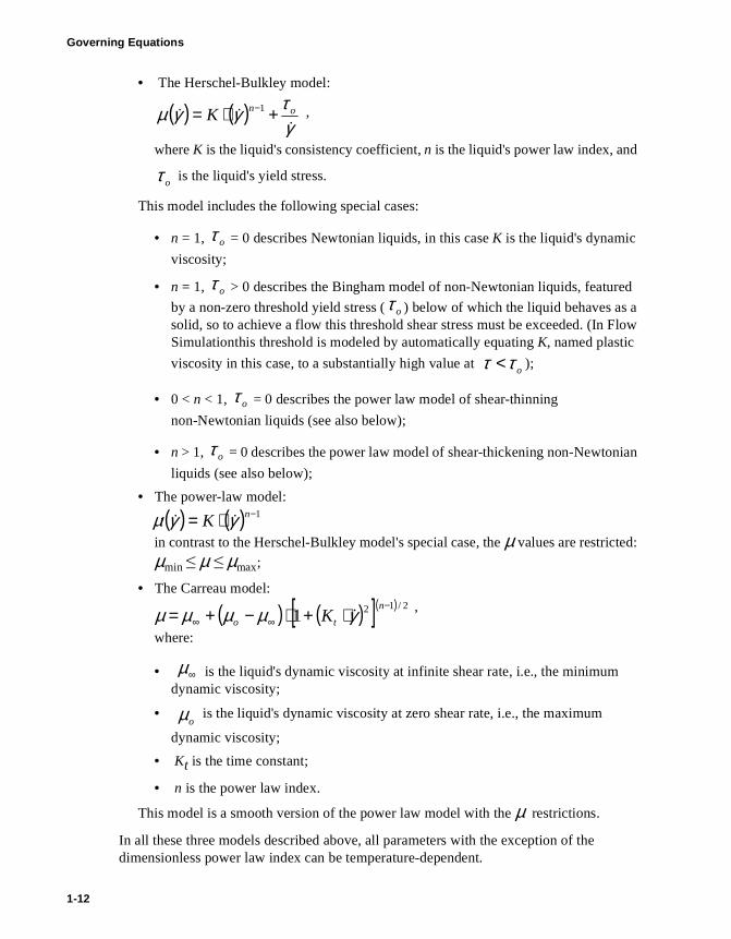
• The Herschel-Bulkley model:
where K is the liquid's consistency coefficient, n is the liquid's power law index, and
is the liquid's yield stress.
This model includes the following special cases:
• n = 1, = 0 describes Newtonian liquids, in this case K is the liquid's dynamic
viscosity;
• n = 1, > 0 describes the Bingham model of non-Newtonian liquids, featured
by a non-zero threshold yield stress ( ) below of which the liquid behaves as a solid, so to achieve a flow this threshold shear stress must be exceeded. (In Flow Simulationthis threshold is modeled by automatically equating K, named plastic
viscosity in this case, to a substantially high value at );
• 0 < n < 1, = 0 describes the power law model of shear-thinning
non-Newtonian liquids (see also below);
• n > 1, = 0 describes the power law model of shear-thickening non-Newtonian
liquids (see also below);
• The power-law model:
in contrast to the Herschel-Bulkley model's special case, the µ values are restricted:
µmin ≤ µ ≤ µmax;
• The Carreau model:
where:
• is the liquid's dynamic viscosity at infinite shear rate, i.e., the minimum dynamic viscosity;
• is the liquid's dynamic viscosity at zero shear rate, i.e., the maximum
dynamic viscosity;
• Kt is the time constant;
• n is the power law index.
( ) ( )γτγγµ&
&& onK +⋅= −1 ,
oτ
oτ
oτoτ
oττ <
oτ
oτ
( ) ( ) 1−⋅= nK γγµ &&,
( ) ( )[ ]( ) 2/121−
∞∞ ⋅+⋅−+=n
to K γµµµµ &,
∞µ
oµ
1-12
This model is a smooth version of the power law model with the µ restrictions.
In all these three models described above, all parameters with the exception of the dimensionless power law index can be temperature-dependent.
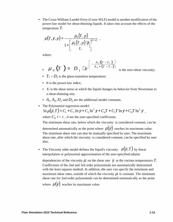
• The Cross-William-Landel-Ferry (Cross-WLF) model is another modification of the power-law model for shear-thinning liquids. It takes into account the effects of the temperature T:
,
where:
• is the zero-shear viscosity;
• T* = D2 is the glass-transition temperature;
• n is the power-law index;
• τ* is the shear stress at which the liquid changes its behavior from Newtonian to
a shear-thinning one;
• A1, A2, D1 and D2 are the additional model constants.
• The Polynomial regression model:
,
where Ci, i = 1…6 are the user-specified coefficients.
The minimum shear rate, below which the viscosity is considered constant, can be
determined automatically as the point where reaches its maximum value. The minimum shear rate can also be manually specified by user. The maximum shear rate, after which the viscosity is considered constant, can be specified by user also.
• The Viscosity table model defines the liquid's viscosity by linear interpolation or polynomial approximation of the user-specified tabular
dependencies of the viscosity µ on the shear rate at the various temperatures T. Coefficients of the 2nd and 3rd order polynomials are automatically determined with the least squares method. In addition, the user can specify the minimum and maximum shear rates, outside of which the viscosity µ is constant. The minimum shear rate for 2nd order polynomials can be determined automatically as the point
where reaches its maximum value.
( ) ( )( ) ( )n
pT
pTpT −
⋅+
= 1
*
0
0
,1
,,,
τγµ
µγµ&
&
( )( )( )
−+
−⋅−
⋅= *2
*1
10TTA
TTA
eDTµ
( ) γγγγγµ &&&&& 2654
2321 lnlnlnln,ln TCTCTCCCCT +++++=
( )γµ &
( )T,γµ &
γ&
( )γµ &
Flow Simulation 2010 Technical Reference 1-13

Governing Equations
Equilibrium volume condensation of water from steam
If the gas whose flow is computed includes steam, Flow Simulation can predict an equilibrium volume condensation of water from this steam (without any surface condensation) taking into account the corresponding changes of the steam temperature, density, enthalpy, specific heat, and sonic velocity. In accordance with the equilibrium approach, local mass fraction of the condensed water in the local total mass of the steam and the condensed water is determined from the local temperature of the fluid, pressure, and, if a multi-component fluid is considered, the local mass fraction of the steam. Since this model implies an equilibrium conditions, the condensation has no history, i.e. it is a local fluid property only.
In addition, it is assumed that
• the volume of the condensed water is neglected, i.e. considered zero, so this prediction works properly only if the volume fraction of the condensed water does not exceed 5%,
• the steam temperature falls into the range of 283...610 K and the pressure does not exceed 10 MPa.
Mass Transfer in Fluid Mixtures
The mass transfer in fluid mixtures is governed by species conservation equations. The equations that describe concentrations of mixture components can be written as
Here Dmn, are the molecular and turbulent matrices of diffusion, Sm is the rate of
production or consumption of the m-th component.
In case of Fick's diffusion law:
The following obvious algebraic relation between species concentrations takes place:
( ) ( ) M 1,2,..., , =+
∂∂+
∂∂=
∂∂+
∂∂
mSx
yDD
xyu
xt
ym
i
ntmnmn
imi
i
m ρρ (1.25)
Dmnt
σµδδ t
mntmnmnmn D DD ⋅=⋅= , (1.26)
∑ =m
my 1 . (1.27)
1-14

Rotation
Global Rotating Reference Frame
The rotation of the coordinate system is taken into account via the following mass-distributed force:
where eijk is the Levy-Civita symbols (function), Ω is the angular velocity of the
rotation, r is the vector coming to the point under consideration from the nearest point lying on the rotation axis.
Local rotating regions
This option is employed for calculating time-dependent (transient) or steady-state flows in regions surrounding rotating non-axisymmetrical solids (e.g. impellers, mixers, propellers, etc), when a single global rotating reference cannot be employed. For example, local rotating regions can be used in analysis of the fluid flow in the model including several components rotating over different axes and/or at different speeds or if the computational domain has a non-axisymmetrical (with respect to a rotating component) outer solid/fluid interface. In accordance with the employed approach, each rotating solid component is surrounded by an axisymmetrical (with respect to the component's rotation axis) Rotating region, which has its own coordinate system rotating together with the component. If the model includes several rotating solid components having different rotation axes, the rotating regions surrounding these components must not intersect with each other. The fluid flow equations in the stationary (non-rotating) regions of the computational domain are solved in the inertial (non-rotating) Cartesian Global Coordinate System. The influence of the rotation's effect on the flow is taken into account in the equations written in each of the rotating coordinate systems.
ikjijkrotationi rueS 22 Ω+Ω−= ρρ ,
Flow Simulation 2010 Technical Reference 1-15

Governing Equations
To connect solutions obtained within the rotating regions and in non-rotating part of the computational domain, special internal boundary conditions are set automatically at the fluid boundaries of the rotating regions. Since the coordinate system of the rotating region rotates, the rotating region’s boundaries are sliced into rings of equal width as shown on the Fig.1.2. Then the values of flow parameters transferred as boundary conditions from the adjacent fluid regions are averaged circumferentially over each of these rings.
To solve the problem, an iterative procedure of adjusting the flow solutions in the rotating regions and in the adjacent non-rotating regions, therefore in the entire computational domain, is performed with relaxations.
Please note that even in case of time-dependent (transient) analysis the flow parameters within the rotating regions are calculated using a steady-state approach and averaged on the rotating regions' boundaries as described above.
Conjugate Heat Transfer
Flow Simulation allows to predict simultaneous heat transfer in solid and fluid media with energy exchange between them. Heat transfer in fluids is described by the energy conservation equation (1.3) where the heat flux is defined by (1.16). The phenomenon of anisotropic heat conductivity in solid media is described by the following equation:
Fig.1.2
Computational domain or fluid subdomainFlow parameters are calculated in the inertial Global Coordinate System
Rotation axisFlow parameters areaveraged over these rings
Local rotating regionFlow parameters are calculatedin the local rotating coordinatesystem
Hi QTe +
∂∂=∂ λρ
(1.28),
1-16
ii xxt ∂∂∂

where e is the specific internal energy, e = c·T, c is specific heat, QH is specific heat
release (or absorption) per unit volume, and λi are the eigenvalues of the thermal conductivity tensor. It is supposed that the heat conductivity tensor is diagonal in the considered coordinate system. For isotropic medium λ1 = λ2 = λ3 = λ.If a solid consists of several solids attached to each other, then the thermal contact resistances between them (on their contact surfaces), specified in the Engineering database
in the form of contact conductance (as m2·K/W), can be taken into account when calculating the heat conduction in solids. As a result, a solid temperature step appears on the contact surfaces. In the same manner, i.e. as a thermal contact resistance, a very thin layer of another material between solids or on a solid in contact with fluid can be taken into account when calculating the heat conduction in solids, but it is specified by the material of this layer (its thermal conductivity taken from the Engineering database) and thickness. The surface heat source (sink) due to Peltier effect may also be considered (see "Thermoelectric Coolers" on page 1-39).
The energy exchange between the fluid and solid media is calculated via the heat flux in the direction normal to the solid/fluid interface taking into account the solid surface temperature and the fluid boundary layer characteristics, if necessary.
If a solid medium is porous with a fluid flowing through it, then a conjugate heat transfer problem in this porous-solid/fluid medium can be solved also in the manner described below. The equations (1.3) and (1.28) are solved in a usual way, but with addition of energy exchange between the fluid and the porous solid matrix, defined via the volumetric
heat exchange in the Eq. (1.28) in a form of , where γ is the
user-defined volumetric coefficient of heat transfer between fluid and the porous matrix, Tp is the temperature of the porous matrix, T is the fluid temperature, and the same QH
with the opposite sign is employed in Eq. (1.28) for the porous matrix. Note that the γ and c of the porous matrix used in Eq. (1.28) can differ from those of the corresponding bulk solid material. Naturally, both the fluid flow equations and the porous matrix heat transfer equation take into account the fluid and solid densities multiplied by the corresponding fluid and solid volume fractions in the porous matrix.
Joule Heating by Electric Current in Solids
This feature is available for the Electronics module users only.
Flow Simulation is able to calculate steady-state (and quasi time-dependent) direct electric current in electroconductive solids. In presence of the electric current, the corresponding
specific Joule heat QJ [W/m3] is released and included in QH of heat transfer equation
(1.28) (see "Conjugate Heat Transfer" on page 1-16). In the case of isotropic material QJ is
( )TTQ PporosityH −⋅γ=
Flow Simulation 2010 Technical Reference 1-17
(1.29)QJ = r·i2,

Governing Equations
where r is the solids' electrical resistivity [Ω·m] (it can be temperature-dependent) and i is
the electric current density [A/m2].
The electric current density vector
is determined via the electric potential ϕ [V]. To obtain the electric potential ϕ, Flow Simulation utilizes the steady-state Laplace equation
Here rii is the temperature-dependent electrical resistivity in the i-th coordinate direction.
Transient electric problems with boundary conditions depending on time are considered as quasi-steady-state. In this case the steady-state problem for potential is solved at each time step, not taking into account transient electrical processes in solids.
The Laplace equation is solved numerically in the computational subdomain (it may be a part of the overall computational domain) of electroconductive materials. This computational subdomain automatically excludes dielectric solids and fluid areas inside. The total electric current in normal direction over a surface In [A] or electric potential
ϕ [V] may be specified by user as boundary conditions for the problem. These conditions may be imposed on surfaces between fluid/electroconductive solid, electroconductive solid/electroconductive solid, dielectric solid/electroconductive solid, and outer solid surfaces. If no electrical boundary conditions are specified by user, the In = 0 boundary condition is automatically specified by default on bounding surfaces.
A surface between electroconductive solids in the computational subdomain is either considered zero-resistance (default) or the electric contact resistance is specified on it. The resistance value is either given explicitly or calculated from the given material and its thickness.
A contact resistance specified on a surface implies that the current passing through it produces the corresponding Joule heating, which yields the following surface heat source
QJS [W/m2]:
where in is the electric current density normal to the surface and ∆ϕ is the electric potential drop at this surface.
The anisotropic electrical resistivity of electroconductive solids can be anisotropic, i.e.
,1
,1
,1
333222111
∂∂
∂∂
∂∂−=
xrxrxr
ϕϕϕi (1.30)
01 =
∂∂
∂∂
iiii xrx
ϕ(1.31)
(1.32)QJS = in·∆ϕ·,··D
1-18
specified by its components in the coordinate system's directions ri , i = 1, 2, 3. The
isotropic/anisotropic type of material is specified for electrical resistivity and thermal conductivity simultaneously, i.e. so that their main axes coincide.

Radiation Heat Transfer Between Solids
In addition to heat conduction in solids, Flow Simulation is capable of calculating radiation heat transfer between solids which surface emissivity is specified. If necessary, a heat radiation from the computational domain far-field boundaries or the model openings can also be defined and considered either as thermal, i.e. by specifying the boundaries emissivity and temperature, or as a solar radiation defined by the specified location (on the surface of the Earth) and time (including date) or by a constant or time-dependent direction and intensity.
Depending on the following conditions, two different approaches are used:
If the heat radiation absorption in solids or radiation spectrum are not considered in the analysis, the radiative heat transfer is calculated using the Ray Tracing approach.
If the heat radiation absorption in solids or radiation spectrum are considered, the Discrete Ordinates method is used.1
Ray Tracing
General Assumptions
The heat radiation from the solid surfaces, both the emitted and reflected, is assumed diffuse (except for the symmetry radiative surface type), i.e. obeying the Lambert law, according to which the radiation intensity per unit area and per unit solid angle is the same in all directions.
The solar radiation is absorbed and reflected by surfaces independently from thermal radiation from all other heat radiation sources.
The propagating heat radiation passes through a solid specified as radiation transparent without any refraction and/or absorption. A solid can be specified as transparent to the solar radiation only, or transparent to the thermal radiation from all sources except the solar radiation, or transparent to both types of radiation, thermal and solar.
The project fluids neither emit nor absorb heat radiation (i.e., they are transparent to the heat radiation), so the heat radiation concerns solid surfaces only.
The radiative solid surfaces which are not specified as a blackbody or whitebody are assumed an ideal graybody, i.e. having a continuous emissive power spectrum similar to that of blackbody, so their monochromatic emissivity is independent of the emission wavelength. For certain materials with certain surface conditions, the graybody emissivity can depend on the surface temperature.
Flow Simulation 2010 Technical Reference 1-19
1. Capabilities and features marked with are available for the HVAC module users
only.

Governing Equations
The Ray Tracing Method
In a general case, the surfaces participating in the heat radiation (hereinafter radiative surfaces) can emit, absorb, and reflect a heat radiation (both the solar and thermal). The heat radiation leaving a radiative surface or radiation source is defined as:
for thermal radiation,
where: ε is the surface emissivity, σ is the Stefan-Boltzmann constant, T is the
temperature of the surface (ε·σ·T 4 is the heat radiated by this surface in accordance with the Stefan-Boltzmann law), qT,i is the incident thermal radiation arriving at this surface,
ρT is the surface reflectivity for thermal radiation (ρT = 1 - ε for graybody walls and ρ =
0 for diffusive radiation sources);
and
for solar radiation,
where: ρs is the surface reflectivity for solar radiation determined from the solar
absorptance α as ρT = 1 - α (ρT = 1 for graybody walls and ρ = 0 for solar radiation
sources), qS,i is the incident solar radiation arriving at this surface.
The total heat radiation q leaving the surface, which is determined as:
q = qT + qS ;
and the net radiation qN being the difference between the heat radiation leaving this surface and the incident heat radiation qi = qT,i + qS,i arriving at it:
qN = q - qi = (qT + qS) - (qT,i + qS,i);
are calculated for each of the surfaces participating in the radiation heat transfer.
In order to reduce the of memory requirements, the problem of determining the leaving and net heat radiation fluxes is solved using a discrete ray Monte-Carlo approach consisting of the following main elements:
To reduce the number of radiation rays and, therefore, the required calculation time and resources, the computational mesh cells containing faces approximating the radiative surfaces are joined in clusters by a special procedure that takes into account the face area and angle between normal and face in each partial cell. The cells intersected by boundaries between radiative surfaces of different emissivity are considered as belonging to one of these surfaces and cannot be combined in one cluster. This procedure is executed after constructing the computational mesh before the calculation and after each solution-adaptive mesh refinement, if any.
iTTT qTq ,4 ⋅+⋅⋅= ρσε
iSSS qq ,⋅= ρ
1-20
From each cluster, a number of rays are emitted, equally distributed over the enclosing unit hemisphere. Each ray is traced through the fluid and transparent solid bodies until

it intercepts the computational domain’s boundary or a cluster belonging to another radiative surface, thus defining a ‘target’ cluster. Since the radiation heat is transferred along these rays only, their number and arrangement govern the accuracy of calculating the radiation heat coming from one radiative surface to another (naturally, the net heat radiated by a radiative surface does not depend on number of these rays). So, for each of the clusters, the hemisphere governed by the ray’s origin and the normal to the face at this origin is uniformly divided into several nearly equal solid angles generated by several zenith angles (at least 3 within the 0...90° range, including the zero zenith angle of the normal to the face) and several azimuth angles (at least 12 within the 0...360° range).
The total number of emitted rays is
,
where m is the number of different latitude values for the rays (including the polar ray),
n is the number of different longitude values (n = 2 for 2D case),
Θ and Φ are the zenith (latitudinal) and azimuth (longitudinal) angles, respectively.
The value of m is defined directly by the View factor resolution level which can be changed by the user via the Calculation Control Options dialog box. The value of n
depends on m as follows: .
The higher the View factor resolution level, the better the accuracy of the radiation heat transfer calculation, but the calculation time and required computer resources increase significantly when high values of View factor resolution level are specified.
Fig.1.3Definition of rays emitted from cluster.
( ) 11 +⋅−= nmN
4⋅= mn
Flow Simulation 2010 Technical Reference 1-21
Periodically during the calculation, a radiation ray is emitted in each of the solid angles in a direction that is defined randomly within this solid angle. These radiation rays are traced until intersection with either another radiative surface or the boundary of the

Governing Equations
computational domain. To increase the accuracy of heat radiation calculation, the number of radiation rays emitted from each cluster can be increased automatically during the calculation, depending on the surface temperature and emissivity, to equalize the radiation heat emitting through the solid angles.
When a radiation ray intercepts a cluster of other radiative surfaces, the radiation heat carried by this ray is uniformly distributed over the area of this cluster. The same procedure is performed if several radiation rays hit the same cluster. To smooth a possible non-uniformity of the incident radiation heat distribution over a radiative surface, a fraction of the radiation heat arriving with rays at a cluster can be transferred to the neighboring clusters also. In addition, small fluctuations are smoothed by the heat conduction in solid regions.
View Factor Calculation
The view factor between two clusters is the fraction of the total radiation energy emitted from one of the clusters that is intercepted by other clusters. The following relations are used in the code to define the view factor.
3D case
View factor for each ray (except for the polar ray) are defined as follows:
, , .
View factor for the Polar ray is:
.
2D case
, , .
.
Set of Equations
is the incident thermal radiation flux;
nF k
k
ε= ( ) ( )2
1112
+⋅−
⋅−=nm
nkkε 1,...,2,1 −= mk
( )( )
21
11 1polar
m nF
m n
− ⋅= − − ⋅ +
2k
kFε= ( ) ( ) ( )
−
−⋅⋅
−⋅
⋅= 12122
sin122
sin2 kmmk
ππε 1,...,2,1 −= mk
( )
−−⋅=12
1cos
m
mFpolar
π
= qFQ
1-22
∑k
kiTkiiT ,,,,
is the incident solar radiation flux;
for thermal radiation;
for solar radiation.
Please note that for the sake of simplicity the set of equations described here defines the radiation heat transfer between clusters only and does not take into account the outer boundaries radiation and radiation sources such as environment, diffusive and solar radiation. In the full set of equations these sources are also considered.
Environment and Solar Radiation
Environmental and solar radiation can be applied to external and internal problems. In fact, the environment radiation is the non-directional energy flux generated by the walls of an imaginary huge ’room’ that surrounds the body. This flux has predefined radiation parameters.
In contrast to the environment radiation, the solar radiation is modeled by the directional energy flux. Therefore, the solar radiation is defined via its power flow (intensity) and its directional vector. In addition to the solar radiation from the computational domain boundaries, a solar radiation source emitting directional radiation can be specified.
The external radiation view factor can be calculated as , where Fi are the
view factors for the rays that have reached the boundaries of the computational domain, and S is the cluster area. Each solar radiation source produces one ray that follows the directional vector. After it reaches the outer boundary or the surface having appropriate
radiation boundary condition, the view factor can be estimated as .
Discrete OrdinatesThis feature is available for the HVAC module users only.
General Assumptions
The whole 4π directional domain at any location within the computational domain is discretized into the specified number of equal solid angles.
Radiation absorptive (semi-transparent) solids absorb and emit heat radiation in
∑=k
kiSkiiS qFQ ,,,,
4,,,,, )( kk
kkiTkikTkT TqFq σερ =− ∑
0)( ,,,,, =− ∑k
kiSkikSkS qFq ρ
SFFk
k ⋅=∑
( ) SnnF clustsolar ⋅= ,
Flow Simulation 2010 Technical Reference 1-23
accordance with the specified solid material absorption coefficient. Scattering is not considered.

Governing Equations
Surfaces of opaque solids absorb the incident heat radiation in accordance with their specified emissivity coefficients, the rest incident radiation is reflected specularly or diffusively, or both specularly and diffusively, in accordance with the specified specularity coefficient.
Radiation absorptive solids reflect radiation specularly, the radiation is refracted in accordance with the specified refraction indices of the solid and adjacent medium (another radiation absorptive solid, or a tarnsparent solid or fluid, which refraction index is always considered as equal to 1). The refraction index value cannot exceed 4.
The Discrete Ordinates Method
In the discrete ordinates method the radiation transfer equation is solved for a set of
discrete directions representing the directional domain of 4π at any position within the
computational domain defined by the position vector . The directional domain is broken down into the specified number of equal solid angles or directions. The total number of directions is defined as:
where RL is the Discretization level specified by the user. Within each direction the radiation intensity is considered constant.
In the absence of scattering the radiation transfer equation can be written as:
where I is the radiation intensity per solid angle, is the blackbody radiation
intensity, k is the medium absorption coefficient, n is the refraction index.
At the surfaces of opaque solids the incident heat radiation is absorbed depending on the specified emmisivity coefficient, the rest of the incident radiation is reflected specularly or diffusively, or both specularly and diffusively. The surface specularly (fs) defines the
fraction of reflected radiaiton, which is reflected specularly, and the diffusively reflected fraction is determined as (1 - fs). The opaque surfaces can also emit heat radiation diffusively in accordance with the surface temperature and the specified emissivity coefficient.
sr
rr
( )2
18
+⋅⋅= RLRLNord
( ) ( ) ( )[ ]rsIrInds
rsdIb
rrrrr
,, 2 −⋅⋅= κ (1.33)
πσ 4T
Ib =
1-24
The absorptive (semi-transparent) solids absorb heat radiation in accordance with the specified absorption coefficient. At the interface between two absorptive (semi-transparent) solids or between an absorptive solid and a fluid the incident radiation changes its direction in accordance with the Snell’s law:

’
where n1 and n2 are the refractive indices of the first and second medium (n is always
equal to 1 for a fully transparent solid or fluid) and θ1 and θ2 are the incident and
refraction angles correspondingly.
The radiation reflection at the interface between two absorptive (semi-transparent) solids or between an absorptive solid and a fluid follows the Fresnel’s relation for unpolarized light:
,
where ρ is the reflectivity which define the fraction of reflected radiation.
The fraction of radiation transmitted through the interface is defined as:
τ = 1 - ρ .
Since all fluids are considered as transparent to heat radiation, the heat radiation propagates through them, as well as through transparent solids, without any interaction with them. However, as the heat radiation is traced through the computational domain by the discrete ordinates method, the ’false scattering’ effect caused by the discretization inaccuracies can appear - it is similar to the ’numerical diffusion’ effect in fluid flow calculations. Creating a finer computational mesh allows to reduce this effect.
When the radiation propagates from a small source to a significant distance, the ’ray effect’ can be encountered as a result of breaking down the directional domain into several directions . As radiation in these directions is traced from the source, it begin to demonstrate a ray-like behavior because more and more cells fall within the same direction with the distance and the radiation intensity distribution within the direction becomes non-uniform. This effect must be considered when decreasing the cell size to
2
1
1
2
sin
sin
n
n=
θθ
θ2
θ1s sr
st
Fig.1.4Radiation reflection at the interface between two abrosptive media.
medium 1
medium 2
( )( )
( )( )
+−
++−
=21
221
2
212
212
sin
sin
tan
tan
2
1)(
θθθθ
θθθθρ s
Flow Simulation 2010 Technical Reference 1-25
avoid the ’false scattering’ effect, so the discretization level must be increased if the finer mesh is used.

Governing Equations
Radiation SpectrumThis feature is available for the HVAC module users only.
Spectrum can be specified for radiation from the computational domain boundaries and for radiation sources set on surfaces of opaque solids (representing openings). Specifying the spectrum for a radiation source or radiation from the far-field boundaries automatically selects the discrete ordinates method for calculating the radiative heat transfer.
The radiation spectrum is considered as consisting of several bands, which edges are specified by the user. Properties of radiation sources, surfaces and materials are considered constant within each band. The wavelength-dependent properties of solid materials are averaged over the specified spectrum bands, so it is recommended to specify the band edges at the wavelengths, at which the material properties change substantially.
If the radiation spectrum is considered, the equation (1.33) takes the following form:
where is the heat radiation intensity in the i-th spectrum band, is the intensity of
the blackbody radiation in the i-th spectrum band, is the specified the medium
absorption coefficient in the i-th spectrum band.
Radiative Surface and Radiation Source Types
Radiative Surfaces
A radiative surface can only be specified on the surface of an opaque solid.
Radiative surface or radiation source type Specified values Dependent values
Wall ε, T, fs ρ = 1-ε, α = ε, fd = 1-fs
Symmetry (ideal reflection) No parameters
Absorbent wall No parameters
Wall to ambient ε, T, fs ρ = 1-ε, α = ε, fd = 1-fs
Non-radiating No parameters
(1.34)( ) ( ) ( )[ ]rsIrInkds
rsdIiii
i
b
rrrrr
,,
λλ2
λλ −⋅⋅=
iIλ ibI λ
ikλ
1-26
For the Wall and Wall to ambient boundary condition, the program gets T from the current results set.

The rays are emitted only from surfaces and boundaries on which the Wall or radiation source conditions are applied.
Surfaces with the specified Absorbent wall boundary condition are taken into account during the calculation but they can act as absorptive surfaces only. This wall type takes all heat from the radiation that reaches it and does not emit any heat.
The Symmetry boundary condition forces the walls to which it is applied to reflect rays as an ideal mirror.
Wall to ambient reproduces the most elementary phenomenon among the radiation effects. The walls with this condition does not interact with any other surfaces. They can only exhaust energy into the space that surrounds the computational domain. Heat flux from such surface could be calculated as:
,
where is the temperature of the environmental radiation.
When a ray reaches the surface of a radiation source or the Wall to ambient surface, it disappears. All energy carried by this ray also dies away.
Non-radiating boundary condition removes specific surfaces from the radiation heat transfer analysis, so they do not affect the results.
The Absorbent wall and Non-radiating surface types of radiative surfaces are not consistent with the Discrete ordinates method, and are substituted in the calculation with Whitebody wall, which emissivity is considered equal to 0 (i.e. to that of whitebody), so that the surface fully reflects all the incident radiation (in accordance with the Lambert law) and does not emit any heat by itself.
Radiation Sources
A radiation source can only be specified on the surface of an opaque solid. All the incident radiation disappears without absorption or reflection on the radiation source surface, unless there is a radiative surface condition defined on the same surface.
Diffusive radiation source Power (Q) or Intensity (I) or T and/or spectruma
a. The spectrum definition is available for the HVAC module users only.
Solar radiation source n, Power (Q) or Intensity (I) or Tb
b. The spectrum of a solar radiation source is always the pre-defined Daylight Spectrum (available for the HVAC module users only).
( )44outout TTQ ⋅−⋅= εσ
outT
Flow Simulation 2010 Technical Reference 1-27

Governing Equations
The solar radiation source makes the wall to emit radiation like the outer solar radiation. It is specified by the direction vector and power or intensity or temperature. The solar radiation at the computational domain boundaries can be specified not only by the direction vector and intensity, but also by the location (on the surface of the Earth) and time.
Simultaneous Use of Radiative Surface and Radiation Source Conditions
The user can specify a radiative surface and radiation source on the same surface of an opaque solid. In this case the total heat radiation leaving the surface is determined as:
q = (1 - ε) qi + ε·σ·T 4 + qsource,
where: ε is the emmisivity of the radiative surface, qi is the incident heat radiation
arriving on the surface, T is the surface temperature and qsource is the heat radiation
emitted by the radiation source. Please note that the raditive surface emmisivity coefficient and temperature do not influence the heat radiation emitted by the radiation source defined on the same surface - the radiation source properties are specified independently.
Viewing Results
The main result of the radiation heat transfer calculation is the solids’ surface or internal temperatures. But these temperatures are also affected by heat conduction in solids and solid/fluid heat transfer. To see the results of radiation heat transfer calculation only, the user can view the Leaving radiant flux and distribution of Net radiant flux over the selected radiative surfaces at Surface Plots. User can also see the maximum, minimum, and average values of these parameters as well as the Leaving radiation rate and Net radiation rate as an integral over the selected surfaces in Surface Parameters. All these parameters can be viewed separately for the solar radiation and radiation from solar radiation sources (solar radiation) and the radiation from all other heat radiation sources (thermal radiation).
When the absorptive (semi-transparent) solids are considered, the additional parameters such as Absorption volume radiant flux, Net volume radiant flow and Net volume radiant flux become available both for the solar and thermal radiation, as well as for the total radiation and heat flux.
1-28

Flows in Porous Media
Porous media are treated in Flow Simulation as distributed resistances to fluid flow, so they can not occupy the whole fluid region or fill the dead-end holes. In addition, if the Heat conduction in solids option is switched on, the heat transfer between the porous solid matrix and the fluid flowing through it is also considered. Therefore, the porous matrix act on the fluid flowing through it via the Si, Siui, and (if heat conduction in solids is considered) QH terms in Eqs. (1.2) and (1.3), whose components related to porosity are
defined as:
where k is the resistance vector of the porous medium (see below), γ is the user-defined volumetric porous matrix/fluid heat transfer coefficient, Tp is the temperature of the
porous matrix, T is temperature of the fluid flowing through the matrix, and the other designations are given in Section 1. In addition, the fluid density in Eqs. (1.1)-(1.3) is multiplied by the porosity n of the porous medium, which is the volume fraction of the interconnected pores with respect to the total medium volume.
In the employed porous medium model turbulence disappears within a porous medium and the flow becomes laminar.
If the heat conduction in porous matrix is considered, then, in addition to solving Eqs. (1.1)-(1.3) describing fluid flow in porous medium, an Eq. (1.28) describing the heat conduction in solids is also considered within the porous medium. In this equation the source QH due to heat transfer between the porous matrix and the fluid is defined in the same manner as in Eq. (1.36), but with the opposite sign. The values of γ and c for the porous matrix may differ from those of the corresponding bulk solid material and hence must be specified independently. Density of the solid material is multiplied by the solid volume fraction in the porous matrix, i.e. by (1-n).
Thermal conductivity of the porous matrix can be specified as anisotropic in the same manner as for the solid material.
The conjugate heat transfer problem in a porous medium is solved under the following restrictions:
• heat conduction in a porous medium not filled with a fluid is not considered,
• porous media are considered transparent for radiation heat transfer,
• heat sources in the porous matrix can be specified in the forms of heat generation
jijporous
i ukS ρδ−= , (1.35)
, (1.36)( )TTQ PporosityH −⋅γ=
Flow Simulation 2010 Technical Reference 1-29
rate or volumetric heat generation rate only; heat sources in a form of constant or time-dependent temperature can not be specified.

Governing Equations
To perform a calculation in Flow Simulation, you have to specify the following porous medium properties: the effective porosity of the porous medium, defined as the volume fraction of the interconnected pores with respect to the total medium volume. Later on, the permeability type of the porous medium must be chosen among the following:
• isotropic (i.e., the medium permeability is independent of direction),
• unidirectional (i.e., the medium is permeable in one direction only),
• axisymmetrical (i.e., the medium permeability is fully governed by its axial and transversal components with respect to a specified direction),
• orthotropic (i.e., the general case, when the medium permeability varies with direction and is fully governed by its three components determined along three principal directions).
Then you have to specify some constants needed to determine the porous medium resistance to fluid flow, i.e., vector k defined as k = - grad(P)/(ρ ·V), where P, ρ, and V are fluid pressure, density, and velocity, respectively. It is calculated according to one of the following formulae:
• k = ∆P·S/(m·L), where ∆P is the pressure difference between the opposite sides of a sample parallelepiped porous body, m is the mass flow rate through the body, S and L are the body cross-sectional area and length in the selected direction, respectively. You can specify ∆P as a function of m, whereas S and L are constants. Instead of mass flow rate you can specify volume flow rate, v. In this case Flow Simulation calculates m = v·ρ. All these values do not specify the porous body for the calculation, but its resistance k only.
• k = (A·V+B)/ρ, where V is the fluid velocity, A and B are constants, ρ is the fluid density. Here, only A and B are specified, since V and ρ are calculated.
• k= µ/(ρ ·D2), where µ and ρ are the fluid dynamic viscosity and density, D is the reference pore size determined experimentally. Here, only D is specified, since µ and ρ are calculated.
• k= µ/(ρ ·D2)·f(Re), differing from the previous formula by the f(Re) factor, yielding a more general formula. Here, in addition to D, f(Re) as a formula dependency is specified.
To define a certain porous body, you specify both the body position in the model and, if the porous medium has a unidirectional or axisymmetrical permeability, the reference directions in the porous body.
1-30

Perforated Plates in Boundary Conditions
This feature is available for the Electronics module users only.
A perforated plate is a particular case of porous media treated in Flow Simulation as distributed hydraulic resistances. Flow Simulation allows to specify a perforated plate as a special feature imposed on a pressure-opening- or fan-type flow boundary condition (see "Boundary Conditions and Engineering Devices" on page 1-36) via the Perforated Plates option. With the use of this feature, the user specifies a perforated plate via its porosity ε (defined as the fraction of the plate area covered by holes) and the holes' shape and size (holes may be either round with specified diameter, or rectangular with specified width and height, or regular polygons with specified side length and number of vertices). Then it can be assigned to any of the abovementioned flow boundary conditions as a distributed hydraulic resistance yielding the additional pressure drop at this boundary
where ρ is the fluid density, u is the fluid velocity inside the plate's holes, and ζ is the perforated plate's hydraulic resistance, calculated according to Ref. 2 fnom the plate porosity ε and the Reynolds number of the flow in the holes:
where Dh = 4·F/Π is the hole hydraulic diameter defined via the area of a single hole F and its perimeter Π, and µ is the fluid's dynamic viscosity. Please note that the ζ (Re, ε) dependence taken from Ref. 2 and employed in Flow Simulation is valid for non-swirled, normal-to-plate flows only.
Cavitation
A liquid subjected to a low pressure below some threshold ruptures and forms vaporous cavities. More specifically, when the local pressure at a point in the liquid falls below the saturation pressure at the local temperature, the liquid undergoes phase transition and form cavities filled with the vapour with an addition of gas that has been dissolved in the liquid. This phenomenon is called cavitation.
The following models of cavitation are available in Flow Simulation:
• Engineering cavitation model (for pre-defined water only):This model employs a homogeneous equilibrium approach and is available for pre-defined water only. It has the capability to account for the thermal effects.
• Isothermal cavitation model:This model is based on the approach considering isothermal, two-phase flows. The
2u·2
1·p ρζ∆ −= , (1.37)
(1.38)Re = ρ·u·Dh/µ,
Flow Simulation 2010 Technical Reference 1-31
isothermal cavitation model is only available for user-defined incompressible liquids.

Governing Equations
Engineering cavitation model (for pre-defined water only)
The homogeneous equilibrium approach is employed. It is applicable for a variety of important industrial processes.
The fluid is assumed to be a homogeneous gas-liquid mixture with the gaseous phase consisting of the vapour and non-condensable (dissolved) gas. The vapour mass fraction is defined at the local equilibrium thermodynamic conditions. The dissolved gas mass fraction is a constant, which can be modified by user.
The velocities and temperatures of the gaseous (including vapour and non-condensable gas) and liquid phases are assumed to be the same.
The density of the gas-liquid mixture is calculated as:
, ,
where v is the specific volume of the gas-liquid mixture, vl is the specific volume of
liquid, zv (T,P) is the vapour compressibility ratio, Runiv is the universal gas constant,
P is the local static pressure, T is the local temperature, yv is the mass fraction of vapour,
µv is the molar mass of vapour, yg is the mass fraction of the non-condensable gas; µg is
the molar mass of the non-condensable gas. The properties of the dissolved non-condensable gas are set to be equal to those of air. By default, the mass fraction of
non-condensable gas is set to 10-5. This is a typical model value appropriated in most
cases but it can be modified by the user in the range of 10-4…10-8.
The mass fraction of vapour yv is computed numerically from the following non-linear
equation for the full enthalpy gas-liquid mixture:
,
where temperature of the mixture T is a function of pressure P and yv. Here hg, hl, hv are
the enthalpies of non-condensable gas, liquid and vapour, respectively, k is the turbulent energy,
is the squared impulse.
The model has the following limitations and recommendations:
• Cavitation is available only for pre-defined water (when defining the project fluids you should select Water from the list of Pre-Defined liquids).
v
1=ρv
vunivvlvg
g
univg P
PTTzRyPTvyy
P
TRyv
µµ),(
),()1( +−−+=
kvI
PThyPThyyPThyH Cvvlvggg 2
52
),(),()1(),(2
+++−−+=
222 )()()( zyxC uuuI ρρρ ++=
1-32
• For mixtures of different liquids the cavitation option cannot be selected.
• The temperature and pressure ranges in the cavitation area must be within the following bounds:
T = 277.15 - 583.15 K, P = 800 - 107 Pa.
• The model does not describe the detailed structure of the cavitation area, i.e. parameters of individual vapour bubbles.
• The volume fraction of vapour is limited by 0.9. The parameters of the flow at the inlet boundary conditions must satisfy this requirement.
• The Cavitation option is not applicable if you calculate a water flow in the model without flow openings (inlet and outlet).
• The fluid region where cavitation occurs must be well resolved by the computational mesh.
• If the calculation has finished or has been stopped and the Cavitation option has been enabled or disabled, the calculation cannot be resumed or continued and must be restarted from the beginning.
Isothermal cavitation model
This model provides a capability to analyze two-phase flows of industrial liquids which thermophysical properties are not described in details.
In the isothermal cavitation model the following assumptions are made:
• The process temperature is constant and the thermal effects are not considered.
• The liquid phase is an incompressible fluid.
• When liquid turns into vapour completely the vapour and non-condensable gas density is defined by the ideal gas law.
• The fluid contains non-condensable (dissolved) gas. One of the four gases can be used as dissolved gas: Air, Carbon dioxide, Helium and Methane. By default, the
non-condensable gas is Air and the mass fraction is set to 10-4. This is a typical model value appropriated in most cases but it can be modified by the user in the
range of 10-2...10-6.
The density of the gas-liquid mixture is calculated as:
,
( )g
g
univ
E
yTR
TPP µρ
0
00−=
LV PPP ≤≤
Flow Simulation 2010 Technical Reference 1-33

Governing Equations
where Runiv is the universal gas constant, P is the local static pressure, PL is the local
static pressure at which the vapour appears, PV is the local static pressure at which the
liquid turns into the vapour completely, T0 is the local temperature, P0E is the saturation
pressure at T0, yg is the mass fraction of the non-condensable gas; µg is the molar mass of
the non-condensable gas.
Two-phase (fluid + particles) Flows
Flow Simulation calculates two-phase flows as a motion of spherical liquid particles (droplets) or spherical solid particles in a steady-state flow field. Flow Simulation can simulate dilute two-phase flows only, where the particle’s influence on the fluid flow (including its temperature) is negligible (e.g. flows of gases or liquids contaminated with particles). Generally, in this case the particles mass flow rate should be lower than about 30% of the fluid mass flow rate.
Fig.1.4 Density-pressure phase diagram
1-34

The particles of a specified (liquid or solid) material and constant mass are assumed to be spherical. Their drag coefficient is calculated with Henderson’s formula (Ref. 3), derived for continuum and rarefied, subsonic and supersonic, laminar, transient, and turbulent flows over the particles, and taking into account the temperature difference between the fluid and the particle. The particle/fluid heat transfer coefficient is calculated with the formula proposed in Ref. 4. If necessary, the gravity is taken into account. Since the particle mass is assumed constant, the particles cooled or heated by the surrounding fluid change their size. The interaction of particles with the model surfaces is taken into account by specifying either full absorption of the particles (that is typical for liquid droplets impinging on surfaces at low or moderate velocities) or ideal or non-ideal reflection (that is typical for solid particles). The ideal reflection denotes that in the impinging plane defined by the particle velocity vector and the surface normal at the impingement point, the particle velocity component tangent to surface is conserved, whereas the particle velocity component normal to surface changes its sign. A non-ideal reflection is specified by the two particle velocity restitution (reflection) coefficients, en and eτ, determining values of these particle velocity components after reflection, V2,n and V2,τ, as their ratio to
the ones before the impingement, V1,n and V1,τ:
As a result of particles impingement on a solid surface, the total erosion mass rate, RΣerosion, and the total accretion mass rate, RΣaccretion, are determined as follows:
,
,
where:N is the number of fractions of particles specified by user as injections in Flow Simulation (the user may specify several fractions of particles, also called injections, so that the particle properties at inlet, i.e. temperature, velocity, diameter, mass flow rate, and material, are constant within one fraction),i is the fraction number,Mp i is the mass impinging on the model walls in unit time for the i-th particle fraction,
Ki is the impingement erosion coefficient specified by user for the i-th particle fraction,Vp i is the impingement velocity for the i-th particle fraction,
b is the user-specified velocity exponent (b = 2 is recommended), f1 i (αp i) is the user-specified dimensionless function of particle impingement angle αp i,
f2 i (dp i) is the user-specified dimensionless function of particle diameter dp i.
n,1Vn,2V
ne =ττ
τ,1V,2V
e =
ipipi2ipi1b
ip
N
1i Mierosion md)d(f)(fVKR
ip
&⋅⋅⋅=∑ ∫=
∑ α
∑=
∑ =N
1iipaccretion MR
Flow Simulation 2010 Technical Reference 1-35

Governing Equations
Boundary Conditions and Engineering Devices
Internal Flow Boundary Conditions
For internal flows, i.e., flows inside models, Flow Simulation offers the following two options of specifying the flow boundary conditions: manually at the model inlets and outlets (i.e. model openings), or to specify them by transferring the results obtained in another Flow Simulation calculation in the same coordinate system (if necessary, the calculation can be performed with another model, the only requirement is the flow regions at the boundaries must coincide).
With the first option, all the model openings are classified into "pressure" openings, "flow" openings, and "fans", depending on the flow boundary conditions which you intend to specify on them.
A "pressure" opening boundary condition, which can be static pressure, or total pressure, or environment pressure is imposed in the general case when the flow direction and/or magnitude at the model opening are not known a priori, so they are to be calculated as part of the solution. Which of these parameters is specified depends on which one of them is known. In most cases the static pressure is not known, whereas if the opening connects the computational domain to an external space with known pressure, the total pressure at the opening is known. The Environment pressure condition is interpreted by Flow Simulation as a total pressure for incoming flows and as a static pressure for outgoing flows. If, during calculation, a vortex crosses an opening with the Environment pressure condition specified at it, this pressure considered as the total pressure at the part of opening through which the flow enters the model and as the static pressure at the part of opening through which the flow leaves the model.
Note that when inlet flow occurs at the "pressure" opening, the temperature, fluid mixture composition and turbulence parameters have to be specified also.
A "flow" opening boundary condition is imposed when dynamic flow properties (i.e., the flow direction and mass/volume flow rate or velocity/ Mach number) are known at the opening. If the flow enters the model, then the inlet temperature, fluid mixture composition and turbulence parameters must be specified also. The pressure at the opening will be determined as part of the solution. For supersonic flows the inlet pressure must be specified also.
A "fan" condition simulates a fan installed at a model opening. In this case the dependency of volume flow rate on pressure drop over the fan is prescribed at the opening. These dependencies are commonly provided in the technical documentation for the fans being simulated.
1-36
With the second option, you specify the boundary conditions by transferring the results obtained in another Flow Simulation calculation in the same coordinate system. If necessary, the calculation can be performed with another model, the only requirement is the flow regions at the boundaries must coincide. At that, you select the created boundary conditions’ type: either as for external flows (so-called "ambient" conditions, see the next Section), or as for "pressure" or "flow" openings, see above. If a conjugate heat transfer problem is solved, the temperature at the part of the boundary lying in a solid body is transferred from the other calculation.
Naturally, the flow boundary conditions specified for an internal flow problem with the first and/or second options must be physically consistent with each other, so it is expedient to specify at least one "pressure"-type boundary condition and at least one "flow"-type boundary condition, if not only "ambient" boundary conditions are specified.
External Flow Boundary Conditions
For external problems such as flow over an aircraft or building, the parameters of the external incoming flow (so-called "ambient" conditions) must be defined. Namely the velocity, pressure, temperature, fluid mixture composition and turbulence parameters must be specified. Evidently, during the calculation they can be partly violated at the flow boundary lying downstream of the model.
Wall Boundary Conditions
In Flow Simulation the default velocity boundary condition at solid walls corresponds to the well-known no-slip condition. The solid walls are also considered to be impermeable. In addition, the wall surface's translation and/or rotation (without changing the model's geometry) can be specified. If a calculation is performed in a rotating coordinate system, then some of the wall surfaces can be specified as stationary, i.e. a backward rotation in this coordinate system (without changing the model geometry). Flow Simulation also provides the "Ideal Wall" condition that corresponds to the well-known slip condition. For example, Ideal Walls can be used to model planes of flow symmetry.
If the flow of non-Newtonian liquids is considered, then the following slip condition at all solid walls can be specified for each non-Newtonian liquid in the project separately: if the shear stress τ exceeds the yield stress value τ0,slip, then
a slip velocity vslip is determined from , where C1 and C2, as well
as τ0,slip, are specified by user.
If conjugate heat transfer in fluid and solid media is not considered, one of the following boundary conditions can be imposed at solid walls: either the wall temperature
2Cslip0,1slip )τ(τCv −=
wTT = (1.39),
Flow Simulation 2010 Technical Reference 1-37

Governing Equations
or the heat flux,
being positive for heat flows from fluid to solid, equal to zero for adiabatic (heat-insulated) walls, and negative for heat flows from solid to fluid.
When considering conjugate heat transfer in fluid and solid media, the heat exchange between fluid and solid is calculated by Flow Simulation, so heat wall boundary conditions are not specified at the walls.
Internal Flow Boundary Conditions
If one or several non-intersecting axisymmetric rotating regions (local rotating reference frames) are specified, the flow parameters are transferred from the adjacent fluid regions and circumferentially averaged over rotating regions’ boundaries as boundary conditions.
Periodic Boundary Conditions
The "periodicity" condition may be applied if the model consist of identical geometrical features arranged in periodic linear order. Periodic boundary conditions are specified at the pair of computational domain boundaries for the selected direction in which a geometrical feature or a group of features repeats regularly over distance. Periodic boundary conditions allows to reduce the analysis time by calculating the fluid flow only for a small group of identical geometrical features or even just for one feature, but taking into account influence of other identical features in the pattern. Please note that the number of basic mesh cells along the direction in which the "periodicity" condition is applied must be no less than five.
Heat Pipes
This feature is available for the Electronics module users only.
"Heat Pipe" is a device (of arbitrary form: a tube, a plate, etc.) transferring heat from its hotter surface to its colder surface due to evaporating a liquid (water, etc.) and condensing its vapor in this device's inner hollow. This liquid evaporates near this hollow’s hotter surface and its vapour condensates near this hollow’s colder surface. The condensed liquid then returns to the hotter end due to gravity or by a wick. If such a device operates under its design conditions, the heat transfer rate provided by this device exceeds substantially any value achievable by a solid body of similar dimensions.
In Flow Simulation a "Heat Pipe" is modeled simplistically as an extremely heat-conducting body. To model real efficiency of a heat pipe, a non-zero thermal resistance can be assigned to it.
wqq = (1.40)
1-38

Two-resistor Components
This feature is available for the Electronics module users only.
A two-resistor model implemented in Flow Simulation can be used for simplified solving of heat transfer problems in an electronic device with small electronic packages (chips, etc.). A small package is considered as consisting of two flat solid plates: Junction and Case, which are mounted on the Board (see Fig.1.5). The junction represents a die or a chip. The case represents the die's case. The heat conduction through the chip is calculated using the user-specified junction-to-case Qjc (from the junction to the top surface of the
package) and junction-to-board Qjb (from the junction to the board on which it is mounted) thermal resistances (in K/W in SI). The Junction and Case plates are modeled as a high conductivity bodies with heat-insulating side walls, so the only Case's top and Junction's bottom transfer heat to the surroundings.
Thermoelectric Coolers
Thermoelectric cooler (TEC) is a flat sandwich consisting of two plates covering a circuit of p-n semiconductor junctions inside. When a direct electric current (DC) i runs through
this circuit, in accordance with the Peltier effect the a·i·Tc heat, where a is the Seebeck
coefficient, Tc is the TEC's "cold" surface temperature, is pumped from the TEC's "cold"
surface to its "hot" surface (the "cold" and "hot" sides are determined from the DC direction). This heat pumping is naturally accompanied by the Joule (ohmic) heat release at both the TEC surfaces and the heat transfer from the hotter side to the colder (reverse to
the Peltier effect). The ohmic heat release is defined as R·i2/2, where R is the TEC's
electric resistance, while the heat transfer is defined as k·∆T , where k is the TEC's
thermal conductivity, ∆T = Th - Tc , Th is the TEC's "hot" surface temperature. The net
heat transferred from the TEC's "cold" surface to its "hot" surface, Qc, is equal to
Fig.1.5Flow Simulation representation of the two-resistor model.
Flow Simulation 2010 Technical Reference 1-39
,TkiRTiaQ cc ∆⋅−⋅−⋅⋅= 2/2

Governing Equations
Correspondingly, the net heat released at the TEC's "hot" surface, Qh, is equal to
.
In Flow Simulation a TEC is specified by selecting a flat plate (box) in the model, assigning its "hot" face, and applying one of the TECs already defined by user in the Engineering Database. The following characteristics of TEC are specified in the Engineering Database:
• the maximum DC current, imax
• the maximum heat Qcmax transferred at this imax at ∆T = 0
• the maximum temperature difference ∆Tmax, attained at Qc = 0
• the voltage Vmax corresponding to imax.
All of these characteristics are specified for two Th values, in accordance with the
information usually provided by the TEC suppliers. Proceeding from these characteristics, the a(T), R(T), and k(T) linear functions are determined. The functional boundary conditions are specified automatically on the TEC's "cold" and "hot" surfaces, which must be free from other boundary conditions.
The temperature solution inside the TEC and on its surfaces is obtained using a special procedure differing from the standard Flow Simulation calculation procedure for heat conduction in solids.
The TEC's "hot" face must be in contact with other solids, i.e it must not be in contact with any fluid. In addition, it is required that the obtained TEC solution, i.e. Th and ∆T, lie
within the TEC's operating range specified by its manufacturer.
HVAC
Local Mean Age
Local mean age (LMA) is the average timeτ for fluid to travel from the selected inlet opening to the point considering both the velocity and diffusion. It is determined by solving the following equation:
,
TkiRTiaQ hh ∆⋅−⋅+⋅⋅= 2/2
ρτσµ
σµρτ =
∂∂
+
∂∂∑
=
−
3
1i it
ti
i xu
x
1-40
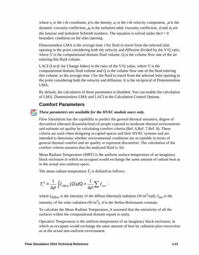
where xi is the i-th coordinate, ρ is the density, ui is the i-th velocity component, µ is the dynamic viscosity coefficient, µt is the turbulent eddy viscosity coefficient, σ and σt are
the laminar and turbulent Schmidt numbers. The equation is solved under theτ = 0 boundary condition on the inlet opening.
Dimensionless LMA is the average time τ for fluid to travel from the selected inlet opening to the point considering both the velocity and diffusion divided by the V/Q ratio, where V is the computational domain fluid volume, Q is the volume flow rate of the air entering this fluid volume.
LACI (Local Air Change Index) is the ratio of the V/Q value, where V is the computational domain fluid volume and Q is the volume flow rate of the fluid entering this volume, to the average time τ for the fluid to travel from the selected inlet opening to the point considering both the velocity and diffusion. It is the reciprocal of Dimensionless LMA.
By default, the calculation of these parameters is disabled. You can enable the calculation of LMA, Dimensionless LMA and LACI in the Calculation Control Options.
Comfort Parameters
These parameters are available for the HVAC module users only.
Flow Simulation has the capability to predict the general thermal sensation, degree of discomfort (thermal dissatisfaction) of people exposed to moderate thermal environments and estimate air quality by calculating comfort criteria (Ref. 6,Ref. 7,Ref. 8). These criteria are used when designing occupied spaces and their HVAC systems and are intended to determine whether environmental conditions are acceptable in terms of general thermal comfort and air quality or represent discomfort. The calculation of the comfort criteria assumes that the analyzed fluid is Air.
Mean Radiant Temperature (MRT) is the uniform surface temperature of an imaginary black enclosure in which an occupant would exchange the same amount of radiant heat as in the actual non-uniform space.
The mean radiant temperature Tr is defined as follows:
,
where Idiffuse is the intensity of the diffuse (thermal) radiation (W/m2/rad), Isun is the
intensity of the solar radiation (W/m2), σ is the Stefan-Boltzmann constant.
To calculate the Mean Radiant Temperature, it assumed that the emissivity of all the surfaces within the computational domain equals to unity.
∑∫ +ΩΩ= sundiffuser IdITσσ 4
1)(
4
14
Flow Simulation 2010 Technical Reference 1-41
Operative Temperature is the uniform temperature of an imaginary black enclosure, in which an occupant would exchange the same amount of heat by radiation plus convection as in the actual non-uniform environment.

Governing Equations
The operative temperature Tc is defined as follows (Ref. 7):
,
where Tr is the mean radiant temperature (°C), T is the fluid temperature (°C), V is the
fluid velocity (m/s).
Predicted Mean Vote (PMV) is an index that predicts the mean value of the votes of a large group of persons on the 7-point thermal sensation scale, based on the heat balance of the human body. Thermal balance is obtained when the internal heat production in the body is equal to the loss of heat to the environment. In a moderate environment, the human thermoregulatory system will automatically attempt to modify skin temperature and sweat secretion to maintain heat balance (Ref. 8).
The predicted mean vote PMV is defined as follows:
,
where
,
,
cold cool slightly cool
neutral slightly warm
warm hot
-3 -2 -1 0 +1 +2 +3
V
VTTT r
c101
10
++
=
( )( ) ( )[ ]
( )[ ] ( ) ( )( ) ( )[ ] ( )
−−+−+⋅−
−−−⋅−−−−−−−⋅−−
⋅+=
−
−
−
−
aclcclrclcl
aa
a
M
TThfTTf
TMpMWM
pWMWM
ePMV
448
5
3
036.0
2732731096.3
340014.05867107.115.5842.0
99.657331005.3
028.0303.0
[ ] )()273()273(1096.3
)(028.07.35448
aclcclrclclcl
cl
TThfTTfI
WMT
−++−+⋅−
−−=−
>+
≤+=
−=
kW
mIforI
kW
mIforI
f
VTTh
clcl
clcl
cl
aclc
2
2
25.0
078.0,645.005.1
078.0,29.100.1
1.12,)(38.2max
1-42
where

M is the metabolic rate (W/m2 of the body area).
It is the rate of transformation of chemical energy into heat and mechanical work by metabolic activities within an organism;
W is the external work (W/m2 of the body area). It accounts for the effective mechanical power;
Icl is the clothing thermal resistance (m2K/W).
It is the resistance to sensible heat transfer provided by a clothing ensemble. The definition of clothing insulation relates to heat transfer from the whole body and, thus, also includes the uncovered parts of the body, such as head and hands. The typical values of thermal resistance for a certain clothing ensemble can be found in Ref. 8;
fcl is the ratio of clothed surface area to nude surface area;
Ta is the air temperature (°C);
Tr is the mean radiant temperature (°C);
v is the relative air velocity (m/s);
pa is the water vapor partial pressure (Pa) calculated in accordance with the saturation curve, the air temperature Ta and the Relative humidity (see "Equilibrium volume
condensation of water from steam" on page 1-14);
hc is the convective heat transfer coefficient (W/m2/K);
Tcl is the clothing surface temperature (°C).
Predicted Percent Dissatisfied (PPD) is an index that provides information on thermal discomfort or thermal dissatisfaction by predicting the percentage of people likely to feel too warm or too cool in a given environment (Ref. 8). It can be obtained from the PMV using the following equation:
.
Draft Temperature is the difference in temperature between any point in the occupied zone and the control condition. "Draft" is defined as any localized feeling of coolness or warmth of any portion of the body due to both air movement and air temperature, with humidity and radiation considered constant. (Ref. 6).
The draft temperature Td is defined as follows:
,
( )24 PMV 0.2179 - PMV 0.03353-exp 95 - 100 PPD =
) 0.1524(V 7.6553TT T md ---=
Flow Simulation 2010 Technical Reference 1-43
where:
T is the local fluid temperature (°C);
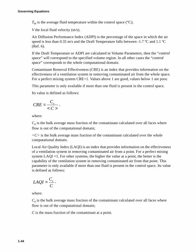
Governing Equations
Tm is the average fluid temperature within the control space (°C);
V the local fluid velocity (m/s).
Air Diffusion Performance Index (ADPI) is the percentage of the space in which the air speed is less than 0.35 m/s and the Draft Temperature falls between -1.7 ºC and 1.1 ºC (Ref. 6).
If the Draft Temperature or ADPI are calculated in Volume Parameters, then the “control space” will correspond to the specified volume region. In all other cases the “control space” corresponds to the whole computational domain.
Contaminant Removal Effectiveness (CRE) is an index that provides information on the effectiveness of a ventilation system in removing contaminated air from the whole space. For a perfect mixing system CRE=1. Values above 1 are good, values below 1 are poor.
This parameter is only available if more than one fluid is present in the control space.
Its value is defined as follows:
,
where:
Ce is the bulk average mass fraction of the contaminant calculated over all faces where flow is out of the computational domain;
<C> is the bulk average mass fraction of the contaminant calculated over the whole computational domain.
Local Air Quality Index (LAQI) is an index that provides information on the effectiveness of a ventilation system in removing contaminated air from a point. For a perfect mixing system LAQI =1. For other systems, the higher the value at a point, the better is the capability of the ventilation system in removing contaminated air from that point. This parameter is only available if more than one fluid is present in the control space. Its value is defined as follows:
,
where:
Ce is the bulk average mass fraction of the contaminant calculated over all faces where flow is out of the computational domain;
C is the mass fraction of the contaminant at a point.
><=
C
CCRE e
C
CLAQI e=
1-44

The Flow Angle calculation is often used to evaluate the performance of a laminar (uni-directional) flow. Consider one of the axis of selected coordinate system as the design flow direction, the results can then be viewed as the deviation from the design. Typically, flow angles of less than 15° might be considered as good.
The flow angle components are defined as follows:
,
where Vx, Vy, Vz are the X, Y, and Z components of the fluid velocity and V is the
absolute value of the fluid velocity vector.
/V)arcos(V (Z) Angle w
/V)arcos(V (Y) Angle w
/V)arcos(V (X) Angle w
z
y
x
===
Flow Simulation 2010 Technical Reference 1-45

Numerical Solution Technique
Numerical Solution Technique
The numerical solution technique employed in Flow Simulation is robust and reliable, so it does not require any user knowledge about the computational mesh and the numerical methods employed. But sometimes, if the model and/or the problem being solved are too complicated, so that the Flow Simulation standard numerical solution technique requires extremely high computer resources (memory and/or CPU time) which are not available, it is expedient to employ Flow Simulation options which allow the adjustment of the automatically specified values of parameters governing the numerical solution technique. To employ these options properly and successfully, take into account the information presented below about Flow Simulation’ numerical solution technique.
Briefly, Flow Simulation solves the governing equations with the finite volume (FV) method on a spatially rectangular computational mesh designed in the Cartesian coordinate system with the planes orthogonal to its axes and refined locally at the solid/fluid interface and, if necessary, additionally in specified fluid regions, at the solid/solid surfaces, and in the fluid region during calculation. Values of all the physical variables are stored at the mesh cell centers. Due to the FV method, the governing equations are discretized in a conservative form. The spatial derivatives are approximated with implicit difference operators of second-order accuracy. The time derivatives are approximated with an implicit first-order Euler scheme. The viscosity of the numerical scheme is negligible with respect to the fluid viscosity.
Computational Mesh
Flow Simulation computational mesh is rectangular everywhere in the computational domain, so the mesh cells’ sides are orthogonal to the specified axes of the Cartesian coordinate system and are not fitted to the solid/fluid interface. As a result, the solid/fluid interface cuts the near-wall mesh cells. Nevertheless, due to special measures, the mass and heat fluxes are treated properly in these cells named partial.
The rectangular computational domain is automatically constructed (may be changed manually), so it encloses the solid body and has the boundary planes orthogonal to the specified axes of the Cartesian coordinate system. Then, the computational mesh is constructed in the following several stages.
First of all, a basic mesh is constructed. For that, the computational domain is divided into slices by the basic mesh planes, which are evidently orthogonal to the axes of the Cartesian coordinate system. The user can specify the number and spacing of these planes along each of the axes. The so-called control planes whose position is specified by user can be among these planes also. The basic mesh is determined solely by the computational domain and does not depend on the solid/fluid interfaces.
1-46

Then, the basic mesh cells intersecting with the solid/fluid interface are split uniformly into smaller cells in order to capture the solid/fluid interface with mesh cells of the specified size (with respect to the basic mesh cells). The following procedure is employed: each of the basic mesh cells intersecting with the solid/fluid interface is split uniformly into 8 child cells; each of the child cells intersecting with the interface is in turn split into 8 cells of next level, and so on, until the specified cell size is attained.
At the next stage of meshing, the mesh obtained at the solid/fluid interface with the previous procedure is refined (i.e. the cells are split further or probably merged) in accordance with the solid/fluid interface curvature. The criterion to be satisfied is established as follows: the maximum angle between the normals to the surface inside one cell should not exceeds certain threshold, otherwise the cell is split into 8 cells.
Finally, the mesh obtained with these procedures is refined in the computational domain to satisfy the so-called narrow channel criterion: for each cell lying at the solid/fluid interface, the number of the mesh cells (including the partial cells) lying in the fluid region along the line normal to the solid/fluid interface and starting from the center of this cell must not be less than the criterion value. Otherwise each of the mesh cells on this line is split into 8 child cells.
As a result of all these meshing procedures, a locally refined rectangular computational mesh is obtained and used then for solving the governing equations on it.
Since all the above-mentioned meshing procedures are performed before the calculation, the obtained mesh is unable to resolve all the solution features well. To overcome this disadvantage, the computational mesh can be refined further at the specified moments during the calculation in accordance with the solution spatial gradients (both in fluid and in solid, see User’s Guide for details). As a result, in the low-gradient regions the cells are merged, whereas in the high-gradient regions the cells are split. The moments of the computational mesh refinement during the calculation are prescribed either automatically or manually.
Spatial Approximations
The cell-centered finite volume (FV) method is used to obtain conservative approximations of the governing equations on the locally refined rectangular mesh. The governing equations are integrated over a control volume which is a grid cell, and then approximated with the cell-centered values of the basic variables. The integral conservation laws may be represented in the form of the cell volume and surface integral equation:
∫∫∫ =⋅+∂∂
dvdsdv QFUt
(1.41)
Flow Simulation 2010 Technical Reference 1-47

Numerical Solution Technique
are replaced by the discrete form
The second-order upwind approximations of fluxes F are based on the implicitly treated modified Leonard's QUICK approximations (Ref. 9) and the Total Variation Diminishing (TVD) method (Ref. 10).
In Flow Simulation, especially consistent approximations for the convective terms, div and grad operators are employed in order to derive a discrete problem that maintains the fundamental properties of the parent differential problem in addition to the usual properties of mass, momentum and energy conservation.
Spatial Approximations at the Solid/fluid Interface
Considering equation (1.42) for partial mesh cells (i.e., for the mesh cells cut by the solid/fluid interface), we introduce the additional boundary faces and the corresponding boundary fluxes taking the boundary conditions and geometry into account (see Fig.1.6), as well as use a special calculation procedure for them. As a result, the solid/fluid interface influence on the problem solution both in the fluid and in the solid is calculated very accurately.
( ) QvSFUv =⋅+∂∂ ∑
facescellt
(1.42)
1-48

Temporal Approximations
Time-implicit approximations of the continuity and convection/diffusion equations (for momentum, temperature, etc.) are used together with an operator-splitting technique (Ref. 11, Ref. 12, and Ref. 13). This technique is used to efficiently resolve the problem of pressure-velocity decoupling. Following the SIMPLE-like approach (Ref. 14), an elliptic type discrete pressure equation is derived by algebraic transformations of the originally derived discrete equations for mass and momentum, and taking into account the boundary conditions for velocity.
Fig.1.6Computational mesh cells at the solid/fluid interface.
Flow Simulation 2010 Technical Reference 1-49

Numerical Solution Technique
Form of the Numerical Algorithm
Let index 'n' denotes the time-level, and '*' denotes intermediate values of the flow parameters. The following numerical algorithm is employed to calculate flow parameters on time-level (n+1) using known values on time-level (n):
ρ* = ρ(pn+δp,T*,y*),
Here U = (ρu, ρT, ρκ, ρε, ρy)Tis the full set of basic variables excluding pressure p,
u=(u1,u2,u3)T is the velocity vector, y = (y1, y2, ..., yM)T is the vector of component
concentrations in fluid mixtures, and δp = pn+1 - pn is an auxiliary variable that is called a pressure correction. These parameters are discrete functions stored at cell centers. They are to be calculated using the discrete equations (1.43)-(1.48) that approximate the governing differential equations. In equations (1.43)-(1.48) Ah, divh, gradh and
Lh = divhgradh are discrete operators that approximate the corresponding differential
operators with second order accuracy.
Equation (1.43) corresponds to the first step of the algorithm when fully implicit discrete convection/diffusion equations are solved to obtain the intermediate values of momentum and the final values of turbulent parameters, temperature, and species concentrations.
The elliptic type equation (1.44) is used to calculate the pressure correction δp. This
equation is defined in such a way that the final momentum field ρun+1 calculated from (1.43) satisfies the discrete fully implicit continuity equation. Final values of the flow parameters are defined by equations (1.45)-(1.48).
( ) nnh SpA
t=+
∆*
*UU
U-U,n
n, (1.43)
( ) ,
tttpL
nh
h ∆−
∆+
∆= ρρρδ
** 1udiv (1.44)
(1.45), 1 pt h
n δρρ grad⋅∆−=+ *uu
,ppp nn δ+=+1 (1.46)
, , , , *1n*1*1n*1 yy ρρρερερκρκρρ ==== ++++ nn TT (1.47)
( ) y 1111 ,, ++++ = nnnn Tpρρ (1.48).
1-50

Methods to Resolve Linear Algebraic Systems
Iterative Methods for Nonsymmetrical Problems
To solve the asymmetric systems of linear equations that arise from approximations of momentum, temperature and species equations (1.43), a preconditioned generalized conjugate gradient method (Ref. 15) is used. Incomplete LU factorization is used for preconditioning.
Iterative Methods for Symmetric Problems
To solve symmetric algebraic problem for pressure-correction (1.44), an original double-preconditioned iterative procedure is used. It is based on a specially developed multigrid method (Ref. 16).
Multigrid Method
The multigrid method is a convenient acceleration technique which can greatly decrease the solution time. Basic features of the multigrid algorithm are as follows. Based on the given mesh, a sequence of grids (grid levels) are constructed, with a decreasing number of nodes. On every such grid, the residual of the associated system of algebraic equations is restricted onto the coarser grid level, forming the right hand side of the system on that grid. When the solution on the coarse grid is computed, it is interpolated to the finer grid and used there as a correction to the result of the previous iteration. After that, several smoothing iterations are performed. This procedure is applied repeatedly on every grid level until the corresponding iteration meets the stopping criteria.
The coefficients of the linear algebraic systems associated with the grid are computed once and stored.
Flow Simulation 2010 Technical Reference 1-51

References
References
1 Reid R.C., Prausnitz J.M., Poling B.E. (1987). The properties of gases and liquids, 4th edition, McGraw-Hill Inc., NY, USA.
2 Idelchik, I.E. (1986). Handbook of Hydraulic Resistance, 2nd edition, Hemisphere, New York, USA.
3 Henderson, C.B. Drag Coefficients of Spheres in Continuum and Rarefied Flows. AIAA Journal, v.14, No.6, 1976.
4 Carlson, D.J. and Hoglund, R.F. Particle Drag and Heat Transfer in Rocket Nozzles. AIAA Journal, v.2, No.11, 1964.
5
6 ASHRAE Handbook–2001 Fundamentals.
7 ISO 7726:1998, Ergonomics of the Thermal Environment – Instruments for Measuring Physical Quantities.
8 ISO 7730:2005, Ergonomics of the thermal environment - Analytical determination and interpretation of thermal comfort using calculation of the PMV and PPD indices and local thermal comfort criteria.
9 Roache, P.J., (1998) Technical Reference of Computational Fluid Dynamics, Hermosa Publishers, Albuquerque, New Mexico, USA.
10 Hirsch, C., (1988). Numerical computation of internal and external flows. John Wiley and Sons, Chichester.
11 Glowinski, R. and P. Le Tallec, (1989). Augmented Lagrangian Methods and Operator-Splitting Methods in Nonlinear Mechanics. SIAM, Philadelphia.
12 Marchuk, G.I., (1982). Methods of Numerical Mathematics, Springer-Verlag, Berlin.
13 Samarskii, A.A., (1989). Theory of Difference Schemes, Nauka, Moscow (in Russian).
14 Patankar, S.V., (1980). Numerical Heat Transfer and Fluid Flow, Hemisphere, Washington, D.C.
15 Saad, Y. (1996). Iterative methods for sparse linear systems, PWS Publishing Company, Boston.
16 Hackbusch, W. (1985). Multi-grid Methods and Applications, Springer-Verlag, NY, USA.
1-52

2
Validation Examples
Introduction
A series of calculation examples presented below validate the ability of Flow Simulation to predict the essential features of various flows, as well as to solve conjugate heat transfer problems (i.e. flow problems with heat transfer in solids). In order to perform the validation accurately and to present clear results which the user can check independently, relatively simple examples have been selected. For each of the following examples, exact analytical expression or well-documented experimental results exist. Each of the examples focus on one or two particular physical phenomena such as: laminar flow with or without heat transfer, turbulent flows including vortex development, boundary layer separation and heat transfer, compressible gas flow with shock and expansion waves. Therefore, these examples validate the ability of Flow Simulation to predict fundamental flow features accurately. The accuracy of predictions can be extrapolated to typical industrial examples (encountered every day by design engineers and solved using Flow Simulation), which may include a combination of the above-mentioned physical phenomena and geometries of arbitrary complexity.
Flow Simulation 2010 Technical Reference 2-1

2-2

1 Flow through a Cone Valve
Let us see how Flow Simulation predicts incompressible turbulent 3D flows in a 3D cone valve taken from Ref.14 (the same in Ref.2) and having a complex flow passage geometry combining sudden 3D contractions and expansions at different turning angles ϕ (Fig. 1.1.). Following the Refs.2 and 14 recommendations on determining a valve’s hydraulic resistance correctly, i.e. to avoid any valve-generated flow disturbances at the places of measuring the flow total pressures upstream and downstream of the valve, the inlet and outlet straight pipes of the same diameter D and of enough length (we take 7D and 17D) are connected to the valve, so constituting the experimental rig model (see Fig. 1.2.). As in Ref.14, a water flows through this model. Its temperature of 293.2 K and fully developed turbulent inlet profile (see Ref.1) with mass-average velocity U ≈ 0.5 m/s (to yield the turbulent flow’s Reynolds number based on the pipe diameter ReD = 105) are specified at the model inlet, and static pressure of 1 atm is specified at the model outlet.
The corresponding model used for these predictions is shown in Fig. 1.2.. The valve’s turning angle ϕ is varied in the range of 0…55° (the valve opening diminishes to zero at ϕ = 82°30´).
Fig. 1.1. The cone valve under consideration: D = 0.206 m, Dax = 1.515D, α = 13°40’.
Fig. 1.2. The model for calculating the 3D flow in the cone valve.
Outlet static pressure
P = 101325 Pa
Inlet velocity profile
Flow Simulation 2010 Technical Reference 2-3
The flow predictions performed with Flow Simulation are validated by comparing the valve’s hydraulic resistance ζv, and the dimensionless coefficient of torque M (see Fig. 1.1.) acting on the valve, m, to the experimental data of Ref.14 (Ref.2).

Since Ref.14 presents the valve’s hydraulic resistance (i.e. the resistance due to the flow obstacle, which is the valve) ζv, whereas the flow calculations in the model (as well as the experiments on the rig) yield the total hydraulic resistance including both ζv and the tubes’ hydraulic resistance due to friction, ζf , i.e. ζ = ζv + ζf , then, to obtain ζv from the flow predictions (as well as from the experiments), ζ f is calculated (measured in the experiments) separately, at the fully open valve (ϕ = 0); then ζv = ζ - ζ f .
In accordance with Ref.14, both ζ and ζf are defined as (Po inlet - Po outlet)/(ρU2/2), where
Po inlet and Po outlet are the flow total pressures at the model’s inlet and outlet, accordingly, ρ is the fluid density. The torque coefficient is defined as m = M/[D3·(ρU2/2)·(1+ ζv)], where M is the torque trying to slew the valve around its axis (vertical in the left picture in Fig. 1.1.) due to a non-uniform pressure distribution over the valve’s inner passage (naturally, the valve’s outer surface pressure cannot contribute to this torque). M is measured directly in the experiments and is integrated by Flow Simulation over the valve’s inner passage.
The Flow Simulation predictions have been performed at result resolution level of 5 with manual setting of the minimum gap size to the valve’s minimum passage in the Y = 0 plane and the minimum wall thickness to 3 mm (to resolve the valve’s sharp edges).
Flow Simulation has predicted ζ f = 0.455, ζv shown in Fig. 1.3., and m shown in Fig. 1.4. It is seen that the Flow Simulation predictions well agree with the experimental data.
This cone valve's 3D vortex flow pattern at ϕ = 45° is shown in Fig. 1.5. by flow trajectories colored by total pressure. The corresponding velocity contours and vectors at the Y = 0 plane are shown in Fig. 1.6.
2-4

0.1
1
10
100
15 20 25 30 35 40 45 50 55ϕ(°)
v
Experimental data
Calculation
Fig. 1.3. Comparison of the Flow Simulation predictions with the Ref.14 experimental data on the cone valve’s hydraulic resistance versus the cone valve turning angle.
Fig. 1.4. Comparison of the Flow Simulation predictions with the Ref.14 experimental data on the cone valve’s torque coefficient versus the cone valve turning angle.
0
0.02
0.04
0.06
0.08
0.1
0.12
0.14
0.16
15 20 25 30 35 40 45 50 55(°)
m
Experimental data
Calculation
Flow Simulation 2010 Technical Reference 2-5
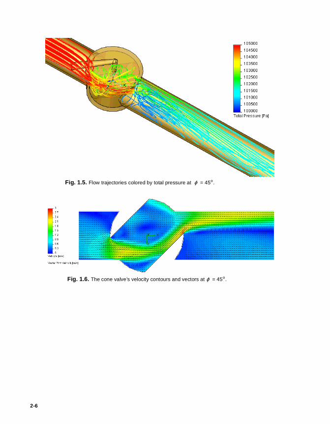
Fig. 1.5. Flow trajectories colored by total pressure at ϕ = 45°.
Fig. 1.6. The cone valve’s velocity contours and vectors at ϕ = 45°.
2-6

2 Laminar Flows Between Two Parallel Plates
Let us consider two-dimensional (planar) steady-state laminar flows of Newtonian, non-Newtonian, and compressible liquids between two parallel stationary plates spaced at a distance of 2h (see Fig. 2.1.).
In the case of Newtonian and non-Newtonian liquids the channel has a 2h = 0.01 m height and a 0.2 m length, the inlet for these liquids have standard ambient temperature (293.2 K) and a uniform inlet velocity profile of uaverage = 0.01 m/s (entrance disturbances are neglected). The inlet pressure is not known beforehand, since it will be obtained from the calculations in accordance with the specified channel exit pressure of 1 atm. (The fluids pass through the channel due to a pressure gradient.)
Since the Reynolds number based on the channel height is equal to about Re2h=100, the flow is laminar.
As for the liquids, let us consider water as a Newtonian liquid and four non-Newtonian liquids having identical density of 1000 kg/m3, identical specific heat of 4200 J/(kgK) and identical thermal conductivity of 10 W/(mK), but obeying different non-Newtonian liquid laws available in Flow Simulation.
The considered non-Newtonian liquids' models and their governing characteristics are presented in Table 2.1. These models are featured by the function connecting the flow shear stress (τ) with the flow shear rate ( ), i.e. , or, following Newtonian liquids, the liquid dynamic viscosity (η) with the flow shear rate ( ), i.e. :
1 the Herschel-Bulkley model: , where K is the consistency coefficient, n is the power-law index, and is the yield stress (a special case with n = 1 gives the Bingham model);
2 the power-law model: , i.e., , which is a special case of Herschel-Bulkley model with = 0;
Fig. 2.1. Flow between two parallel plates.
uaverage or m
γ& ( )γτ &f=γ& ( ) γγητ && ⋅=
( ) onK τγτ +⋅= &
oτ
( )nK γτ &⋅= ( ) 1−⋅= nK γη &oτ
( ) 2/1−n
Flow Simulation 2010 Technical Reference 2-7
3 the Carreau model: , , where is the liquid dynamic viscosity at infinite shear rate, i.e. the minimum dynamic viscosity, is the liquid dynamic viscosity at zero shear rate, i.e. the maximum
γητ &⋅= ( ) ( )[ ]211∞∞ ⋅+⋅−+= o K γηηηη & ∞η
oη

dynamic viscosity, K1 is the time constant, n is the power-law index (this model is a smooth version of the power-law model).
Table 2.1
In accordance with the well-known theory presented in Ref.1, after some entrance length, the flow profile u(y) becomes fully developed and invariable. It can be determined from
the Navier-Stokes x-momentum equation corresponding to
this case in the coordinate system shown in Fig. 2.1. (y = 0 at the channel's center plane,
is the longitudinal pressure gradient along the channel, in the flow under
consideration).
As a result, the fully developed u(y) profile for a Newtonian fluid has the following form:
u(y) = - ,
where η is the fluid dynamic viscosity and η is the half height of the channel,
,
where uaverage is the flow's mass-average velocity defined as the flow's volume flow rate
divided by the area of the flow passage cross section.
For a non-Newtonian liquid described by the power-law model the fully developed u(y) profile and the corresponding pressure gradient can be determined from the following formulae:
Non-Newtonian liquid No. 1 2 3 4
Non-Newtonian liquid model Herschel-Bulkley Bingham Power law Carreau
Consistency coefficient, K (Pa⋅sn) 0.001 0.001 0.001 -Power law index, n 1.5 1 0.6 0.4
Yield stress, (Pa) 0.001 0.001 - -
Minimum dynamic viscosity, (Pa⋅s)
- - - 10-4
Maximum dynamic viscosity, (Pa⋅s)
- - - 10-3
Time constant, K 1 (s) - - - 1
oτ
∞η
oη
hconst
dy
d
dx
dP wττ ===
dx
dP
dy
du=γ&
)(2
1 22 yhdx
dP −η
2
3
h
u
dx
dP average −=
η
+n 1
2-8
, .( )
−
++=
n
average h
y
n
nuyu 1
1
12n
average
n
n
h
u
h
K
dx
dP
+⋅⋅−= 12

For a non-Newtonian liquid described by the Herschel-Bulkley model the fully developed u(y) profile can be determined from the following formulae:
at ,
at ,
where the unknown wall shear stress is determined numerically by solving the
nonlinear equation
,
e.g. with the Newton method, as described in this validation. The corresponding pressure
gradient is determined as .
For a non-Newtonian liquid described by the Carreau model the fully developed u(y) profile can not be determined analytically in an explicit form, so in this validation example it is obtained by solving the following parametric equation:
,
,
where p is a free parameter varied within the ±pmax range,
,
( ) ( ) n
n
oww
n n
n
K
huyu
1
/1max 1
+−
+== ττ
τhy
w
o
ττ<
( )
−
−−⋅=
+n
n
ow
ow h
y
uyu
1
max 1ττ
ττhy
w
o
ττ>
wτ
( )
−+
−⋅−⋅+
⋅=+
w
own
n
oww
naverage n
n
n
n
K
hu
τττττ
τ 121
1
1
/1
hdx
dP wτ=
( )( )2/)1(220 1)(
−∞∞ +−+=
n
w
pph
y λµµµτ
( )( 1) / 22 2 2 20 0max 2 2
( ) ( )11
2 ( 1) ( 1)
n
w w w
h hhu u p p np
n n
µ µ µ µµ λτ τ λ τ λ
−∞ ∞∞ − − = − − + − − + +
( )
+−+=
−
∞∞
2/)1(2max
20max 1)(
n
w pp λµµµτ
( )( 1) / 22 2 2 20 0( ) ( )11
nh hhu p p np
µ µ µ µµ λ−∞ ∞∞ − − = + + − +
Flow Simulation 2010 Technical Reference 2-9
max max max max 2 22 ( 1) ( 1)w w wn nτ τ λ τ λ + +

The p value is varied to satisfy .
The corresponding pressure gradient is equal to .
The SolidWorks model for the 2D calculation is shown in Fig. 2.2.. The boundary conditions are specified as mentioned above and the initial conditions coincide with the inlet boundary conditions. The results of the calculations performed with Flow Simulation at result resolution level 5 are presented in Figs.2.3 - 2.8. The channel exit u(y) profile and the channel P(x) profile were obtained along the sketches shown by green lines in Fig. 2.2..
max
0 0
h p
average
dyhu udy u dp
dp= =∫ ∫
hdx
dP wτ=
Fig. 2.2. The model for calculating 2D flow between two parallel plates with Flow Simulation.
Fig. 2.3. The water and liquid #3 velocity profiles u(y) at the channel outlet.
0
0.002
0.004
0.006
0.008
0.01
0.012
0.014
0.016
-0.005 -0.003 -0.001 0.001 0.003 0.005Y, m
U, m/s
Water, theory
Water, calculation
Power law, theory
Power-law,calculation
2-10

From Figs.2.4, 2.6, and 2.8 you can see that for all the liquids under consideration, after some entrance length of about 0.03 m, the pressure gradient governing the channel pressure loss becomes constant and nearly similar to the theoretical predictions. From Figs.2.3, 2.5, and 2.7 you can see that the fluid velocity profiles at the channel exit obtained from the calculations are close to the theoretical profiles.
Fig. 2.4. The water and liquid #3 longitudinal pressure change along the channel, P(x).
101325
101325.05
101325.1
101325.15
101325.2
101325.25
101325.3
0 0.05 0.1 0.15 0.2X, m
P, Pa
Water, theory
Water, calculation
Power law, theory
Power-law,calculation
Fig. 2.5. The liquids #1 and #2 velocity profiles u(y) at the channel outlet.
0
0.002
0.004
0.006
0.008
0.01
0.012
0.014
0.016
-0.005 -0.003 -0.001 0.001 0.003 0.005 Y, m
U, m/s
Herschel-Bulkley,theoryHerschel-Bulkley,calculation
Bingham, theory
Binham, calculation
Flow Simulation 2010 Technical Reference 2-11

In the case of compressible liquids the channel has the height of 2h = 0.001 m and the length of 0.5 m, the liquids at its inlet had standard ambient temperature (293.2 K) and a uniform inlet velocity profile corresponding to the specified mass flow rate of
= 0.01 kg/s.
Fig. 2.6. The liquids #1 and #2 longitudinal pressure change along the channel, P(x).
101325
101325.1
101325.2
101325.3
101325.4
101325.5
101325.6
0 0.05 0.1 0.15 0.2X, m
P, Pa
Herschel-Bulkley,theoryHerschel-Bulkley,calculation
Bingham, theory
Binham, calculation
Fig. 2.7. The liquid #4 velocity profile u(y) at the channel outlet.
0
0.002
0.004
0.006
0.008
0.01
0.012
0.014
-0.005 -0.003 -0.001 0.001 0.003 0.005 Y, m
U, m/s
Carreau, theory
Carreau,calculation
m&
2-12
The inlet pressure is not known beforehand, since it will be obtained from the calculations as providing the specified mass flow rate under the specified channel exit pressure of 1 atm. (The fluids pass through the channel due to the pressure gradient).

Let us consider two compressible liquids whose density obeys the following laws:
• the power law:
, where ρ0, P0, B and n are specified: ρ0 is the liquid's density under the reference pressure P0, B and n are constants,
• the logarithmic law:
, where ρ0, P0, B and C are specified: ρ0 is the liquid's density under the reference pressure P0, B and C are constants.
In this validation example these law's parameters values have been specified as ρ0=103 kg/m3, P0 = 1 atm, B = 107 Pa, n = 1.4, C = 1, and these liquids have the 1Pa·s dynamic viscosity.
Since this channel is rather long, the pressure gradient along it can be determined as
, where η is the liquids' dynamic viscosity, is the liquid mass flow rate, S is the channel's width, ρ is the liquid density.
Therefore, by substitution the compressible liquids' ρ(P) functions, we obtain the following equations for determining P(x) along the channel:
• for the power-law liquid:
Fig. 2.8. The liquid #4 longitudinal pressure change along the channel, P(x).
101325
101325.02
101325.04
101325.06
101325.08
101325.1
101325.12
101325.14
0 0.05 0.1 0.15 0.2 X, m
P, Pa
Carreau, theory
Carreau, calculation
0 0
nP B
P B
ρρ
+= +
0
0
1 *lnB P
CB P
ρρ = +−+
2
3P m
x h S
ηρ
∂ = −∂
& m&
Flow Simulation 2010 Technical Reference 2-13

its solution is
,
where C1 is a constant determined from the boundary conditions;
• for the logarithmic-law liquid:
, this equation is solved numerically.
Both the theoretical P(x) distributions and the corresponding distributions computed within Flow Simulation on a 5*500 computational mesh are presented in Figs.2.9 and 2.10. It is seen that the Flow Simulation calculations agree with the theoretical distributions.
1/
02
0
3n
P BP m
x h S P B
µρ
+∂ = − ∂ +
&
( ) 1 11
0 120
3( )
1n n
n mP B P B x C
n h S
µρ
++ = + ++
&
20 0
31 ln
P m P BC
x h S P B
µρ
∂ += − −∂ +
&
Fig. 2.9. The logarithmic-law compressible liquid's longitudinal pressure change along the channel, P(x).
0
2000000
4000000
6000000
8000000
10000000
12000000
14000000
16000000
18000000
0 0.1 0.2 0.3 0.4 0.5 X, m
P, Pa
Logarithmic law,theory
Logarithmic law,calculation
2-14

Fig. 2.10. The power-law compressible liquid's longitudinal pressure change along the channel, P(x).
0
5000000
10000000
15000000
20000000
25000000
30000000
35000000
0 0.1 0.2 0.3 0.4 0.5 X, m
P, Pa
Power law, theory
Power law,calculation
Flow Simulation 2010 Technical Reference 2-15

2-16

3 Laminar and Turbulent Flows in Pipes
Let us see how the 3D flow through a straight pipe is predicted. We consider water (at standard 293.2 K temperature) flowing through a long straight pipe with circular cross section of d = 0.1 m (see Fig. 3.1.). At the pipe inlet the velocity is uniform and equal to uinlet. At the pipe outlet the static pressure is equal to 1 atm.
The SolidWorks model used for all the 3D pipe flow calculations is shown in Fig. 3.2. The initial conditions have been specified to coincide with the inlet boundary conditions. The computational domain is reduced to domain (Z ≥ 0, Y ≥ 0) with specifying the flow symmetry planes at Z = 0 and Y = 0.
According to theory (Ref.1), the pipe flow velocity profile changes along the pipe until it becomes a constant, fully developed profile at a distance of Linlet from the pipe inlet. According to Ref.1, Linlet is estimated as:
Fig. 3.1. Flow in a pipe.
uinlet
Fig. 3.2. The SolidWorks model for calculating 3D flow in a pipe with Flow Simulation.
Flow Simulation 2010 Technical Reference 2-17
where Red = ρ·U·d/µ is the Reynolds number based on the pipe diameter d, U is the mass-average flow velocity, ρ is the fluid density, and µ is the fluid dynamic viscosity.

Therefore, to provide a fully developed flow in the pipe at Red under consideration, we will study the cases listed in Table 3.2. Here, Lpipe is the overall pipe length. All the Flow Simulation predictions concerning the fully developed pipe flow characteristics are referred to the pipe section downstream of the inlet section.
*) the lengths in brackets are for the rough pipes.
The flow regime in a pipe can be laminar, turbulent, or transitional, depending on Red. According to Ref.1, Red = 4000 is approximately the boundary between laminar pipe flow and turbulent one (here, the transitional region is not considered).
Theory (Refs. 1 and 4) states that for laminar fully developed pipe flows (Hagen-Poiseuille flow) the velocity profile u(y) is invariable and given by:
where R is the pipe radius, and dP/dx is the longitudinal pressure gradient along the pipe, which is also invariable and equal to:
The Flow Simulation predictions of dP/dx and u(y) of the laminar fully developed pipe flow at Red = 100 performed at result resolution level 6 are presented in Fig. 3.3. and Fig. 3.4. The presented predictions relate to the smooth pipe, and similar ones not presented here have been obtained for the case of the rough tube with relative sand roughness of k/d=0.2…0.4 %, that agrees with the theory (Ref.1).
Table 3.2 Pipe inlet velocities and lengths.
Red uinlet, m/s Linlet, m Lpipe, m
0.1 10-6 0.3 0.45
100 0.001 0.3 0.45
1000 0.01 3 4.5
104 0.1 4 (5)* 6 (10)*
105 1 4 (5)* 6 (10)*
106 10 4 (5)*6 6 (10)*
=⋅=⋅
=⋅≥⋅⋅
610...6000Re,40
6000...2500Re,100
2500...1.0Re,3Re03.0
d
d
dd
d
d
dd
Linlet =
)(4
1)( 22 yR
dx
dPyu −−=
µ,
2
8
R
u
dx
dP inlet−= µ .
2-18

From Fig. 3.3. one can see that after an entrance length of about 0.15 m the pressure gradient predicted by Flow Simulation coincides with the one predicted by theory. Therefore, the prediction of pipe pressure loss is excellent. As for local flow features, from Fig. 3.4. one can see that the fluid velocity profiles predicted at the pipe exit are rather close to the theoretical profile.
101325.0000
101325.0002
101325.0004
101325.0006
101325.0008
101325.0010
101325.0012
101325.0014
101325.0016
101325.0018
101325.0020
0 0.1 0.2 0.3 0.4 0.5 X (m)
Pressure (Pa)
Theory
Calculation
Fig. 3.3. The longitudinal pressure change (pressure gradient) along the pipe at Red ≈ 100.
Fig. 3.4. The fluid velocity profile at the pipe exit for Red ≈ 100.
0
0.0005
0.001
0.0015
0.002
0.0025
0 0.01 0.02 0.03 0.04 0.05 Y (m)
Velocity (m/s)
Theory
Calculation
Flow Simulation 2010 Technical Reference 2-19

The velocity profile and longitudinal pressure distribution in a smooth pipe at Red = 105, i.e., in a turbulent pipe flow regime, predicted by Flow Simulation at result resolution level 6 are presented in Figs.3.5 and 3.6 and compared to theory (Ref.1, the Blasius law of pressure loss, the 1/7-power velocity profile).
Then, to stand closer to engineering practice, let us consider the Flow Simulation predictions of the pipe friction factor used commonly and defined as:
where L is length of the pipe section with the fully developed flow, along which pressure loss ∆P is measured.
101200
101400
101600
101800
102000
102200
102400
0 2 4 6 8 10 X (m)
Pressure (Pa)
Theory
Calculation
Fig. 3.5. The longitudinal pressure change (pressure gradient) along the pipe at Red = 105.
L
d
u
Pf
inlet
⋅∆=
2
2
ρ,
2-20
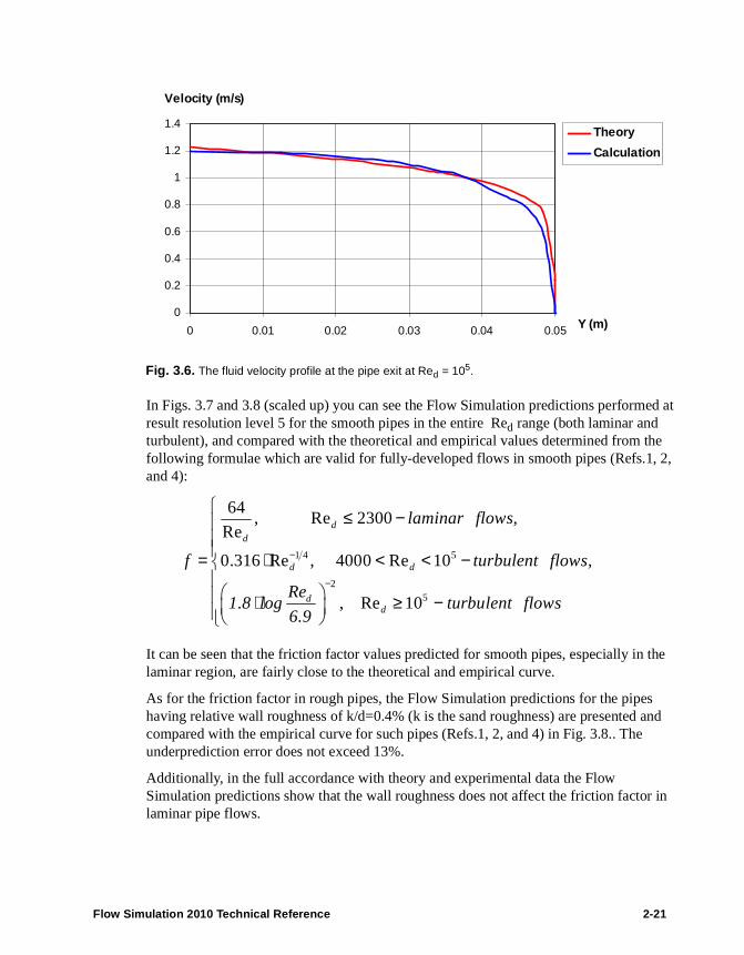
In Figs. 3.7 and 3.8 (scaled up) you can see the Flow Simulation predictions performed at result resolution level 5 for the smooth pipes in the entire Red range (both laminar and turbulent), and compared with the theoretical and empirical values determined from the following formulae which are valid for fully-developed flows in smooth pipes (Refs.1, 2, and 4):
It can be seen that the friction factor values predicted for smooth pipes, especially in the laminar region, are fairly close to the theoretical and empirical curve.
As for the friction factor in rough pipes, the Flow Simulation predictions for the pipes having relative wall roughness of k/d=0.4% (k is the sand roughness) are presented and compared with the empirical curve for such pipes (Refs.1, 2, and 4) in Fig. 3.8.. The underprediction error does not exceed 13%.
Additionally, in the full accordance with theory and experimental data the Flow Simulation predictions show that the wall roughness does not affect the friction factor in laminar pipe flows.
Fig. 3.6. The fluid velocity profile at the pipe exit at Red = 105.
0
0.2
0.4
0.6
0.8
1
1.2
1.4
0 0.01 0.02 0.03 0.04 0.05 Y (m)
Velocity (m/s)
Theory
Calculation
1 4 5
25
64, Re 2300
Re
0.316 Re , 4000 Re 10
, Re 10
dd
d d
dd
laminar flows,
f turbulent flows,
Re1.8 log turbulent flows
6.9
−
−
≤ −
= ⋅ < < − ⋅ ≥ −
Flow Simulation 2010 Technical Reference 2-21

Fig. 3.7. The friction factor predicted by Flow Simulation for smooth pipes in comparison with the theoretical and empirical data (Refs.1, 2, and 4).
1.E-03
1.E-02
1.E-01
1.E+00
1.E+01
1.E+02
1.E+03
1.E-01 1.E+00 1.E+01 1.E+02 1.E+03 1.E+04 1.E+05 1.E+06 Red
Friction factor
Smooth pipes,theoretical andempirical dataCalculation
0.010
0.100
1.E+03 1.E+04 1.E+05 1.E+06Red
Friction Factor
Smooth wall,theoretical andempirical dataSmooth wall,calculation
Rough wall,k/d=0.4%, empiricaldataRough wall,k/d=0.4%,calculation
Fig. 3.8. The friction factor predicted by Flow Simulation for smooth and rough pipes in comparison with the theoretical and empirical data (Refs.1, 2, and 4).
2-22

4 Flows Over Smooth and Rough Flat Plates
Let us consider uniform flows over smooth and rough flat plates with laminar and turbulent boundary layers, so that Flow Simulation predictions of a flat plate drag coefficient are validated.
We consider the boundary layer development of incompressible uniform 2D water flow over a flat plate of length L (see Fig. 4.1.). The boundary layer develops from the plate leading edge lying at the upstream computational domain boundary. The boundary layer at the leading edge is considered laminar. Then, at some distance from the plate leading edge the boundary layer automatically becomes turbulent (if this distance does not exceed L).
The SolidWorks model is shown in Fig. 4.2.. The problem is solved as internal in order to avoid a conflict situation in the corner mesh cell where the external flow boundary and the model wall intersect. In the internal flow problem statement, to avoid any influence of the upper model boundary or wall on the flow near the flat plate, the ideal wall boundary condition has been specified on the upper wall. The plate length is equal to 10 m, the channel height is equal to 2 m, the walls’ thickness is equal to 0.5 m.
Water
L
Fig. 4.1. Flow over a flat plate.
Fig. 4.2. The model for calculating the flow over the flat plate with Flow Simulation.
Outlet
Rough or smooth wall
Ideal wallInlet
Flow Simulation 2010 Technical Reference 2-23

To solve the problem, an incoming uniform water flow of a certain velocity (see below), temperature of 293.2 K, turbulence intensity of 1%, and turbulence length of 0.01 m is specified at the channel inlet, whereas the water static pressure of 1 atm is specified at the channel outlet.
The flow computation is aimed at predicting the flat plate drag coefficient, defined as (see Refs. 1 and 4):
where F is the plate drag force, A is the plate surface area, ρ is fluid density, and V is the fluid velocity.
According to Refs.1 and 4, the plate drag coefficient value is governed by the Reynolds number, based on the distance L from the plate leading edge (ReL = ρVL/µ, where ρ is the fluid density, V is the incoming uniform flow velocity, and µ is fluid dynamic viscosity), as well as by the relative wall roughness L/k, where k is the sand roughness. As a result, Refs.1 and 4 give us the semi-empirical flat plate CD (ReL) curves obtained for different L/k from the generalized tubular friction factor curves and presented in Fig. 4.3. (here, ε ≡ k). If the boundary layer is laminar at the plate leading edge, then the wall roughness does not affect CD until the transition from the laminar boundary layer to the turbulent one, i.e., the CD (ReL) curve is the same as for a hydraulically smooth flat plate. The transition region’s boundaries depend on various factors, the wall roughness among them. Here is shown the theoretical transition region for a hydraulically smooth flat plate. The transition region's boundary corresponding to fully turbulent flows (i.e., at the higher ReL) is marked in Fig. 4.3. by a dashed line. At the higher ReL, the semi-empirical theoretical curves have flat parts along which ReL does not affect CD at a fixed wall roughness. These flat parts of the semi-empirical theoretical curves have been obtained by a theoretical scaling of the generalized tubular friction factor curves to the flat plate conditions under the assumption of a turbulent boundary layer beginning from the flat plate leading edge.
To validate the Flow Simulation flat plate CD predictions within a wide ReL range, we have varied the incoming uniform flow velocity at the model inlet to obtain the ReL values of 105, 3·105, 106, 3·106, 107, 3·107, 108, 3·108, 109.To validate the wall roughness influence on CD, the wall roughness k values of 0, 50, 200, 103, 5·103, 104 µm have been considered. The Flow Simulation calculation results obtained at result resolution level 5 and compared with the semi-empirical curves are presented in Fig. 4.3..
As you can see from Fig. 4.3., CD (ReL) of rough plates is somewhat underpredicted by Flow Simulation in the turbulent region, at L/k ³ 1000 the CD (ReL) prediction error does not exceed about 12%.
AV
FCd
2
2ρ=
,
2-24

Fig. 4.3. The flat plate drag coefficient predicted with Flow Simulation for rough and hydraulically smooth flat plates in comparison with the semi-empirical curves (Refs.1 and 4).
0
0.002
0.004
0.006
0.008
0.01
0.012
0.014
1.00E+05 1.00E+06 1.00E+07 1.00E+08 1.00E+09 Re
CD
L/k=1e3
L/k=2e3
L/k=1e4
L/k=5e4
L/k=2e5
Smooth
Flow Simulation 2010 Technical Reference 2-25

2-26

5 Flow in a 90-degree Bend Square Duct
Following Ref.8, we will consider a steady-state flow of water (at 293.2 K inlet temperature and Uinlet = 0.0198 m/s inlet uniform velocity) in a 40x40 mm square cross-sectional duct having a 90°-angle bend with ri = 72 mm inner radius (ro = 112 mm outer radius accordingly) and attached straight sections of 1.8 m upstream and 1.2 m downstream (see Fig. 5.1.). Since the flow's Reynolds number, based on the duct's hydraulic diameter (D=40 mm), is equal to ReD = 790, the flow is laminar.
The Flow Simulation prediction was performed at result resolution level 7.
The predicted dimensionless (divided by Uinlet) velocity profiles are compared in Figs.5.2, 5.3 with the ones measured with a laser-Doppler anemometry at the following duct cross sections: XH = -5D, -2.5D, 0 (or θ=0°) and at the θ=30°, 60°, 90° bend sections. The z and
r directions are represented by coordinates and , where z1/2 = 20 mm. The
dimensionless velocity isolines (with the 0.1 step) at the duct's θ= 60° and 90° sections, both measured in Ref.8 and predicted with Flow Simulation, are shown in Figs.5.4 and 5.5.
It is seen that the Flow Simulation predictions are close to the Ref.8 experimental data.
Fig. 5.1. The 90°-bend square duct's configuration indicating the velocity measuring stations and the dimensionless coordinates used for presenting the velocity profiles.
o
i o
r r
r r
−− 1/ 2
z
z
Flow Simulation 2010 Technical Reference 2-27

2-28
Fig. 5.2. The duct's velocity profiles predicted by Flow Simulation (red lines) in comparison with the Ref.8 experimental data (circles).

Fig. 5.3. The duct's velocity profiles predicted by Flow Simulation (red lines) in comparison with the Ref.8 experimental data (circles).
z/z1/2=0.5 z/z1/2=0
z/z1/2=0.5 z/z1/2=0
Flow Simulation 2010 Technical Reference 2-29

Fig. 5.4. The duct's velocity isolines at the θ = 60° section predicted by Flow Simulation (left) in comparison with the Ref.8 experimental data (right).
Fig. 5.5. The duct's velocity isolines at the θ =90° section predicted by Flow Simulation (left) in
2-30
comparison with the Ref.8 experimental data (right).

6 Flows in 2D Channels with Bilateral and Unilateral Sudden Expansions
In this example we will consider both turbulent and laminar incompressible steady-state flows through 2D (plane) channels with bilateral and unilateral sudden expansions and parallel walls, as shown in Figs.6.1 and 6.2. At the 10 cm inlet height of the bilateral-sudden-expansion channels a uniform water stream at 293.2 K and 1 m/s is specified. The Reynolds number is based on the inlet height and is equal to Re = 105, therefore (since Re > 104) the flow is turbulent. At the 30 mm height inlet of the unilateral-sudden-expansion channel an experimentally measured water stream at 293.2 K and 8.25 mm/s mean velocity is specified, so the Reynolds number based on the inlet height is equal to Re = 250, therefore the flow is laminar. In both channels, the sudden expansion generates a vortex, which is considered in this validation from the viewpoint of hydraulic loss in the bilateral-expansion channel (compared to Ref.2) and from the viewpoint of the flow velocity field in the unilateral-expansion channel (compared to Ref.13).
Fig. 6.1. Flow in a 2D (plane) channel with a bilateral sudden expansion.
outlet
X
Y
inletWater
1 m/s
Fig. 6.2. Flow in a 2D (plane) channel with a unilateral sudden expansion.
400 mm20 mm
30 m
m
h =
15
Y
X0
Inlet experimental velocity profile Outlet static pressure
recirculation Lr
Flow Simulation 2010 Technical Reference 2-31

Bilateral sudden expansion
In accordance with Ref.2, the local hydraulic loss coefficient of a bilateral sudden expansion (the so-called total pressure loss due to flow) for a turbulent (Re > 104) flow with a uniform inlet velocity profile depends only on the expansion area ratio and is determined from the following formula:
where A0 and A1 are the inlet and outlet cross sectional areas respectively, P0 and P1 are the inlet and outlet total pressures, and ρu0
2/2 is the inlet dynamic head.
In a real sudden expansion the flow hydraulic loss coefficient is equal to ζ = ζf + ζs, where ζf is the friction loss coefficient. In order to exclude ζf from our comparative analysis, we have imposed the ideal wall boundary condition on all of the channel walls.
In this validation example the channel expansion area ratios under consideration are: 1.5, 2.0, 3.0, and 6.0. To avoid disturbances at the outlet due to the sudden expansion, the channel length is 10 times longer than its height. The 1 atm static pressure is specified at the channel outlet.
The ζ s values predicted by Flow Simulation at result resolution level 8 for different channel expansion area ratios A0/A1 are compared to theory in Fig. 6.3.
From Fig. 6.3., one can see that Flow Simulation overpredicts ζ s by about 4.5...7.9 %.
2
1
020
10 1
2
−=−=
A
A
u
PPs ρ
ζ ,
Fig. 6.3. Comparison of Flow Simulation calculations to the theoretical values (Ref.2) for the sudden expansion hydraulic loss coefficient versus the channel expansion area ratio.
0
0.1
0.2
0.3
0.4
0.5
0.6
0.7
0.8
0.9
1
0 0.2 0.4 0.6 0.8 1A0/A1
s
Theory
Calculation
2-32

Unilateral sudden expansion
The model used for the unilateral-sudden-expansion channel's flow calculation is shown in Fig. 6.4. The channel's inlet section has a 30 mm height and a 20 mm length. The channel's expanded section (downstream of the 15 mm height back step) has a 45 mm height and a 400 mm length (to avoid disturbances of the velocity field compared to the experimental data from the channel's outlet boundary condition). The velocity profile measured in the Ref.13 at the corresponding Reh = 125 (the Reynolds number based on the step height) is specified as a boundary condition at the channel inlet. The 105 Pa static pressure is specified at the channel outlet.
The flow velocity field predicted by Flow Simulation at result resolution level 8 is compared in Figs.6.5, 6.6, and 6.7 to the values measured in Ref.13 with a laser anemometer. The flow X-velocity (u/U, where U = 8.25 mm/s) profiles at several X = const (-20 mm, 0, 12 mm, … 150 mm) cross sections are shown in Fig. 6.5. It is seen that the predicted flow velocity profiles are very close to the experimental values both in the main stream and in the recirculation zone. The recirculation zone's characteristics, i.e. its length LR along the channel's wall, (plotted versus the Reynolds number Reh based on the channel's step height h, where Reh =125 for the case under consideration), the separation streamline, and the vortex center are shown in Figs.6.6 and 6.7. It is seen that they are very close to the experimental data.
Fig. 6.4. The SolidWorks model for calculating the 2D flow in the unilateral-sudden-expansion channel with Flow Simulation.
Inlet velocity profile
Outlet static pressure
Flow Simulation 2010 Technical Reference 2-33

As one can see, both the integral characteristics (hydraulic loss coefficient) and local
Fig. 6.5. The unilateral-sudden-expansion channel's velocity profiles predicted by Flow Simulation (red lines) in comparison with the Ref.13 experimental data (black lines with dark circles).
0
2
4
6
8
10
12
0 50 100 150 200 250 Reh
L/h
- r
ecir
cul
atio
n z
one
leng
th
Fig. 6.6. The unilateral-sudden-expansion channel's recirculation zone length predicted by Flow Simulation (red square) in comparison with the Ref.13 experimental data (black signs).
0
5
10
15
0 0.2 0.4 0.6 0.8 1
separation streamlines,calculation
vortex center, calculation
Fig. 6.7. The unilateral-sudden-expansion channel recirculation zone's separation streamlines and vortex center, both predicted by Flow Simulation (red lines and square) in comparison with the Ref.13 experimental data (black signs).
2-34
values (velocity profiles and recirculation zone geometry) of the turbulent and laminar flow in a 2D sudden expansion channel under consideration are adequately predicted by Flow Simulation.

7 Flow over a Circular Cylinder
Let us now consider an external incompressible flow example. In this example, water at a temperature of 293.2 K and a pressure of 1 atm flows over a cylinder of 0.01 m or 1 m diameter. The flow pattern of this example substantially depends on the Reynolds number which is based on the cylinder diameter. At low Reynolds numbers (4 < Re < 60) two steady vortices are formed on the rear side of the cylinder and remain attached to the cylinder, as it is shown schematically in Fig. 7.1. (see Refs.3).
At higher Reynolds numbers the flow becomes unstable and a von Karman vortex street appears in the wake past the cylinder. Moreover, at Re > 60…100 the eddies attached to the cylinder begin to oscillate and shed from the cylinder (Ref.3). The flow pattern is shown schematically in Fig. 7.2..
To calculate the 2D flow (in the X-Y plane) with Flow Simulation, the model shown in Fig. 7.3. has been created. The cylinder diameter is equal to 0.01 m at Re ≤104 and 1 m at Re >104. The incoming stream turbulence intensity has been specified as 1%. To take the flow’s physical instability into account, the flow has been calculated by Flow Simulation using the time-dependent option. All the calculations have been performed at result resolution level 7.
Fig. 7.1. Flow past a cylinder at low Reynolds numbers (4 < Re < 60).
Fig. 7.2. Flow past a cylinder at Reynolds numbers Re > 60…100.
Flow Simulation 2010 Technical Reference 2-35
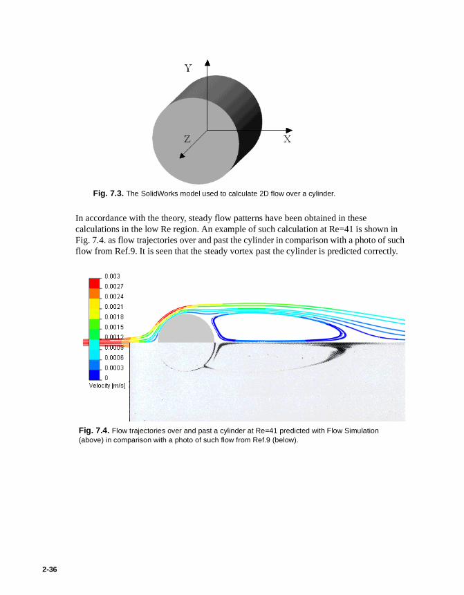
In accordance with the theory, steady flow patterns have been obtained in these calculations in the low Re region. An example of such calculation at Re=41 is shown in Fig. 7.4. as flow trajectories over and past the cylinder in comparison with a photo of such flow from Ref.9. It is seen that the steady vortex past the cylinder is predicted correctly.
Fig. 7.3. The SolidWorks model used to calculate 2D flow over a cylinder.
Fig. 7.4. Flow trajectories over and past a cylinder at Re=41 predicted with Flow Simulation (above) in comparison with a photo of such flow from Ref.9 (below).
2-36

The unsteady vortex shedding from a cylinder at Re > 60..100, yields oscillations of both drag and lateral forces acting on the cylinder and a von Karman vortex street is formed past the cylinder. An X-velocity field over and past the cylinder is shown in Fig. 7.5. The Flow Simulation prediction of the cylinder drag and lateral force oscillations' frequency in a form of Strouhal number (Sh = D/(tU), where D is the cylinder diameter, t is the period of oscillations, and U is the incoming stream velocity) in comparison with experimental data for Re≥103 is shown in Fig. 7.6..
Fig. 7.5. Velocity contours of flow over and past the cylinder at Re=140.
0
0.05
0.1
0.15
0.2
0.25
0.3
0.35
0.4
1.E+01 1.E+02 1.E+03 1.E+04 1.E+05 1.E+06 1.E+07 Re
Sh
Fig. 7.6. The cylinder flow's Strouhal number predicted with Flow Simulation (red triangles) in comparison with the experimental data (blue line with dashes, Ref.4).
Flow Simulation 2010 Technical Reference 2-37
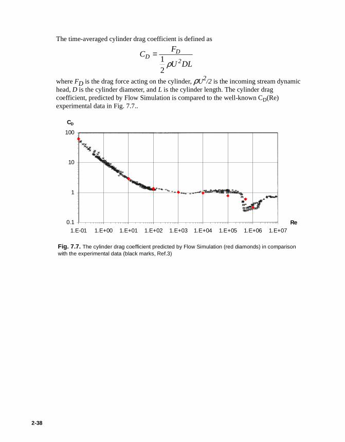
The time-averaged cylinder drag coefficient is defined as
where FD is the drag force acting on the cylinder, ρU2/2 is the incoming stream dynamic head, D is the cylinder diameter, and L is the cylinder length. The cylinder drag coefficient, predicted by Flow Simulation is compared to the well-known CD(Re) experimental data in Fig. 7.7..
DLU
FC
2
DD
ρ21
=
0.1
1
10
100
1.E-01 1.E+00 1.E+01 1.E+02 1.E+03 1.E+04 1.E+05 1.E+06 1.E+07Re
CD
Fig. 7.7. The cylinder drag coefficient predicted by Flow Simulation (red diamonds) in comparison with the experimental data (black marks, Ref.3)
2-38

8 Supersonic Flow in a 2D Convergent-Divergent Channel
Now let us consider an external supersonic flow of air in a 2D (plane) convergent-divergent channel whose scheme is shown on Fig. 8.1.
A uniform supersonic stream of air, having a Mach number M=3, static temperature of 293.2 K, and static pressure of 1 atm, is specified at the channel inlet between two parallel walls. In the next convergent section (see Fig. 8.2.) the stream decelerates through two oblique shocks shown schematically in Fig. 8.1. as lines separating regions 1, 2, and 3. Since the convergent section has a special shape adjusted to the inlet Mach number, so the shock reflected from the upper plane wall and separating regions 2 and 3 comes to the section 3 lower wall edge, a uniform supersonic flow occurs in the next section 3 between two parallel walls. In the following divergent section the supersonic flow accelerates thus forming an expansion waves fan 4. Finally, the stream decelerates in the exit channel section between two parallel walls when passing through another oblique shock.
The SolidWorks model of this 2D channel is shown in Fig. 8.3.
Since the channel was designed for the inviscid flow of an ideal gas, the ideal wall boundary condition has been specified and the laminar only flow has been considered
Fig. 8.1. Supersonic flow in a 2D convergent-divergent channel.
Fig. 8.2. Dimensions (in m) of the 2D convergent-divergent channel including a reference line for comparing the Mach number.
Flow Simulation 2010 Technical Reference 2-39
instead of turbulent. The computed Mach number along the reference line and at the reference points (1-5) are compared with the theoretical values in Fig. 8.4..

To obtain the most accurate results possible with Flow Simulation, the calculations have been performed at result resolution level 8. The predicted Mach number at the selected channel points (1-5) and along the reference line (see Fig. 8.2.), are presented in Table 8.3 and Fig. 8.4. respectively.
Table 8.3 Mach number values predicted with Flow Simulation with comparison to the theoretical values at the reference points.
From Table 8.3 and Fig. 8.4. it can be seen that the Flow Simulation predictions are very close to the theoretical values. In Fig. 8.4. one can see that Flow Simulation properly predicts the abrupt parameter changes when the stream passes through the shock and a fast parameter change in the expansion fan.
Fig. 8.3. The model for calculating the 2D supersonic flow in the 2D convergent-divergent channel with Flow Simulation.
Point 1 2 3 4 5X coordinate of point, m 0.0042 0.047 0.1094 0.155 0.1648Y coordinate of point, m 0.0175 0.0157 0.026 0.026 0.0157
Theoretical M 3.000 2.427 1.957 2.089 2.365Flow Simulation prediction of M 3.000 2.429 1.965 2.106 2.380
Prediction error,% 0.0 0.1 0.4 0.8 0.6
2-40

To show the full flow pattern, the predicted Mach number contours of the channel flow are shown in Fig. 8.5..
This example illustrates that Flow Simulation is capable of capturing shock waves with a high degree of accuracy. This high accuracy is possible due to the Flow Simulation solution adaptive meshing capability. Solution adaptive meshing automatically refines the mesh in regions with high flow gradients such as shocks and expansion fans.
Fig. 8.4. Mach number values predicted with Flow Simulation along the reference line (the reference points on it are marked by square boxes with numbers) in comparison with the theoretical
1.92
2.12.22.32.42.52.62.72.82.9
33.1
0 0.02 0.04 0.06 0.08 0.1 0.12 0.14 0.16 0.18x, m
M
Theory
Calculation
1
2
3
4
5
Fig. 8.5. Mach number contours predicted by Flow Simulation.
Flow Simulation 2010 Technical Reference 2-41

2-42

9 Supersonic Flow over a Segmental Conic Body
Now let us consider an external supersonic flow of air over a segmental conic body shown in Fig. 9.1. The general case is that the body is tilted at an angle of α with respect to the incoming flow direction. The dimensions of the body whose longitudinal (in direction t, see Fig. 9.1.) and lateral (in direction n) aerodynamic drag coefficients, as well as longitudinal (with respect to Z axis) torque coefficient, were investigated in Ref.5 are presented in Fig. 9.2. They were determined from the dimensionless body sizes and the Reynolds number stated in Ref.5.
Fig. 9.1. Supersonic flow over a segmental conic body.
Center of gravity
n
y
xa
t
External air flowM∞ = 1.7
Flow Simulation 2010 Technical Reference 2-43
The model of this body is shown in Fig. 9.3..
Fig. 9.2. Model sketch dimensioned in centimeters.

To compare the Flow Simulation predictions with the experimental data of Ref.5, the calculations have been performed for the case of incoming flow velocity of Mach number 1.7. The undisturbed turbulent incoming flow has a static pressure of 1 atm, static temperature of 660.2 K, and turbulence intensity of 1%. The flow Reynolds number of 1.7x10⁶ (defined with respect to the body frontal diameter) corresponds to these conditions, satisfying the Ref.5 experimental conditions.
To compare the flow prediction with the experimental data of Ref.5, the calculations have been performed for the body tilted at α = 0°, 30°, 60°, 90°, 120°, 150° and 180° angles. To reduce the computational resources, the Z = 0 flow symmetry plane has been specified in all of the calculations. Additionally, the Y = 0 flow symmetry plane has been specified at α = 0° and 180°.
The calculations have been performed at result resolution level 6.
The comparison is performed on the following parameters:
• longitudinal aerodynamic drag coefficient,
where Ft is the aerodynamic drag force acting on the body in the t direction (see Fig. 9.1.), ρU2/2 is the incoming stream dynamic head, S is the body frontal cross section (being
Fig. 9.3. The SolidWorks model for calculating the 3D flow over the 3D segmental conic body with Flow Simulation.
SU
FC
2
tt
ρ21
= ,
2-44
perpendicular to the body axis) area;

• lateral aerodynamic drag coefficient,
where Fn is the aerodynamic drag force acting on the body in the n direction (see Fig. 9.1.), ρU2/2 is the incoming stream dynamic head, S is the body frontal cross section (being perpendicular to the body axis) area;
• on the longitudinal (with respect to Z axis) aerodynamic torque coefficient,
where Mz is the aerodynamic torque acting on the body with respect to the Z axis (see Fig. 9.1.), ρU2/2 is the incoming stream dynamic head, S is the body frontal cross section (being perpendicular to the body axis) area, L is the reference length.
The calculation results are presented in Figs.9.4 and 9.5.
From Fig. 9.4., it is seen that the Flow Simulation predictions of both Cn and Ct are excellent.
SU
FC
2
nn
ρ21
= ,
SLU
Mm
2
zz
ρ2
1=
,
Fig. 9.4. The longitudinal and lateral aerodynamic drag coefficients predicted with Flow Simulation and measured in the experiments of Ref.5 versus the body tilting angle.
-1-0.8-0.6-0.4-0.2
00.20.40.60.8
11.21.41.6
0 30 60 90 120 150 180Attack angle
(degree)
Ct , Cn
Ct experiment
Ct calculation
Cn experiment
Cn calculation
Flow Simulation 2010 Technical Reference 2-45

As for the longitudinal aerodynamic torque coefficient (mz) prediction, it is also close to the experimental data of Ref.5, especially if we take into account the measurements error.
To illustrate the quantitative predictions with the corresponding flow patterns, the Mach number contours are presented in Figs. 9.6, 9.7, and 9.8. All of the flow patterns presented on the figures include both supersonic and subsonic flow regions. The bow shock consists of normal and oblique shock parts with the subsonic region downstream of the normal shock. In the head subsonic region the flow gradually accelerates up to a supersonic velocity and then further accelerates in the expansion fan of rarefaction waves. The subsonic wake region past the body can also be seen.
Fig. 9.5. The longitudinal aerodynamic torque coefficient predicted with Flow Simulation and measured in the experiments (Ref.5) versus the body tilting angle.
-0.04
-0.02
0
0.02
0.04
0.06
0.08
0 30 60 90 120 150 180
Attack angle (degree)
mz
Experiment
Calculation
Fig. 9.6. Mach number contours at α = 0o
.
2-46

Fig. 9.7. Mach number contours at α = 60°.
Fig. 9.8. Mach number contours at α = 90°.
Flow Simulation 2010 Technical Reference 2-47

As the forward part becomes sharper, the normal part of the bow shock and the corresponding subsonic region downstream of it become smaller. In the presented pictures, the smallest nose shock (especially its subsonic region) is observed at a = 60o.
2-48

10 Flow over a Heated Plate
Now let us consider a uniform 2D flows with a laminar boundary layer on a heated flat plate, see Fig. 10.1.. The incoming uniform air stream has a velocity of 1.5 m/s, a temperature of 293.2 K, and a static pressure of 1 atm. Thus, the flow Reynolds number defined on the incoming flow characteristics and on the plate length of 0.31 m is equal to 3.1·104, therefore the boundary layer beginning from the plate’s leading edge is laminar (see Ref.6).
Then, let us consider the following three cases:
Case #1
The plate over its whole length (within the computational domain) is 10°C warmer than the incoming air (303.2 K), both the hydrodynamic and the thermal boundary layer begin at the plate's leading edge coinciding with the computational domain boundary;
Case #2
The upstream half of the plate (i.e. at x ∼ 0.15 m) has a fluid temperature of 293.2 K, and the downstream half of the plate is 10°C warmer than the incoming air (303.2 K), the hydrodynamic boundary layer begins at the plate's leading edge coinciding with the computational boundary;
Case #3
Plate temperature is the same as in case #1, the thermal boundary layer begins at the inlet computational domain boundary, whereas the hydrodynamic boundary layer at the inlet computational domain boundary has a non-zero thickness which is equal to that in case #2 at the thermal boundary layer starting.
The calculation goal is to predict the local coefficient of heat transfer from the wall to the fluid, as well as the local skin-friction coefficient.
Fig. 10.1. Laminar flow over a heated flat plate.
Heated plate
T = 303.2 K
Air flow
V = 1.5 m/s
T = 293.2 K
Computational domain
Flow Simulation 2010Technical Reference 2-49

The SolidWorks model used for calculating the 2D flow over the heated flat plate with Flow Simulation is shown in Fig. 10.2.. The problem is solved as internal in order to avoid the conflict situation when the external flow boundary with ambient temperature conditions intersects the wall with a thermal boundary layer.
To avoid any influence of the upper wall on the flow near the heated lower wall, the ideal wall boundary condition has been specified on the upper wall. To solve the internal problem, the incoming fluid velocity is specified at the channel inlet, whereas the fluid static pressure is specified at the channel exit. To specify the external flow features, the incoming stream's turbulent intensity is set to 1% and the turbulent length is set to 0.01 m, i.e., these turbulent values are similar to the default values for external flow problems.
The heat transfer coefficient h and the skin-friction coefficient Cf are Flow Simulation output flow parameters. The theoretical values for laminar flow boundary layer over a flat plate, in accordance with Ref.6 can be determined from the following equations:
where
k is the thermal conductivity of the fluid,x is the distance along the wall from the start of the hydrodynamic boundary layer,
Fig. 10.2. The SolidWorks model used for calculating the 2D flow over heated flat plate with Flow Simulation.
Inlet velocity Ux
Ideal wall
Heated wall
Static pressure opening
x
kh xNu
= ,
2-50
Nux is the Nusselt number defined on a heated wall as follows:2/1
x3/1
x RePr332.0Nu ⋅=

for a laminar boundary layer if it’s starting point coincides with the thermal boundary layer starting point, and
for a laminar boundary layer if the thermal boundary layer begins at point x0 lying downstream of the hydrodynamic boundary layer starting point, in this case Nux is defined at x>x0 only;
where is the Prandtl number, µ is the fluid dynamic viscosity, Cp is the
fluid specific heat at constant pressure, is the Reynolds number
defined on x, ρ is the fluid density, and V is the fluid velocity;
at , i.e., with a laminar boundary layer.
As for the hydrodynamic boundary layer thickness δ needed for specification at the computational domain boundary in case #3, in accordance with Ref.6, it has been
determined from the following equation: , so δ = 0.00575 m in this
case. For these calculations all fluid parameters are determined at the outer boundary of the boundary layer.
The Flow Simulation predictions of h and Cf performed at result resolution level 7, and the theoretical curves calculated with the formulae presented above are shown in Figs.10.3 and 10.4. It is seen that the Flow Simulation predictions of the heat transfer coefficient and the skin-friction coefficient are in excellent agreement with the theoretical curves.
3 4/30
2/1x
3/1
)x/x(1
RePr332.0
−
⋅=xNu
PrµCp
k----------=
RexρV x
µ-----------=
0,664
RefxC = 5Re 5 10x ≤ ⋅
0.54.64 / Rexxδ = ⋅
Flow Simulation 2010Technical Reference 2-51
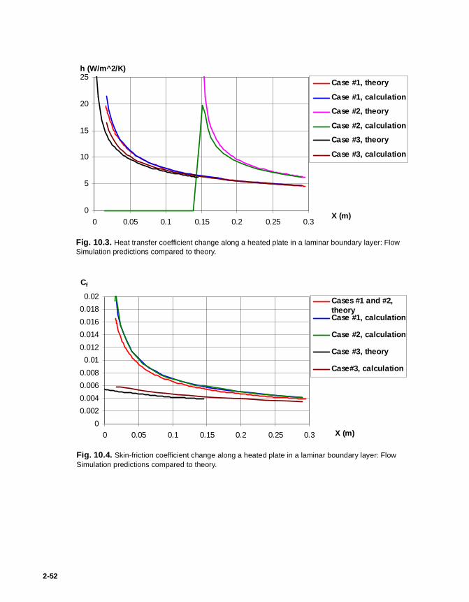
Fig. 10.3. Heat transfer coefficient change along a heated plate in a laminar boundary layer: Flow Simulation predictions compared to theory.
0
5
10
15
20
25
0 0.05 0.1 0.15 0.2 0.25 0.3 X (m)
h (W/m^2/K)
Case #1, theory
Case #1, calculation
Case #2, theory
Case #2, calculation
Case #3, theory
Case #3, calculation
Fig. 10.4. Skin-friction coefficient change along a heated plate in a laminar boundary layer: Flow Simulation predictions compared to theory.
0
0.002
0.004
0.006
0.008
0.01
0.012
0.014
0.016
0.018
0.02
0 0.05 0.1 0.15 0.2 0.25 0.3 X (m)
Cf
Cases #1 and #2,theoryCase #1, calculation
Case #2, calculation
Case #3, theory
Case#3, calculation
2-52

11 Convection and Radiation in an Annular Tube
We will now consider incompressible laminar flow in a portion of an annular tube, whose outer shell is a heat source having constant heat generation rate Q1 with a heat-insulated outer surface, and whose central body fully absorbs the heat generated by the tube’s outer shell (i.e. the negative heat generation rate Q2 is specified in the central body); see Fig. 11.1.. (The tube model is shown in Fig. 11.2.). We will assume that this tube is rather long, so the tube's L=1 m portion under consideration has fully developed fluid velocity and temperature profiles at the inlet, and, since the fluid properties are not temperature-dependent, the velocity profile also will not be temperature-dependent.
Fig. 11.1. Laminar flow in a heated annular tube.
X
Y
ø1.2m
ø0.4m
ø1.4 m
X
Y
1m
Q1 or T1
Q2 or T2
P = 1 atm
U, T
Fig. 11.2. A model created for calculating 3D flow within a heated annular tube using Flow Simulation.
Flow Simulation 2010 Technical Reference 2-53

To validate the Flow Simulation capability for solving conjugate heat transfer problems both with and without radiation, let us solve the following three problems: 1) a conjugate heat transfer problem with convection only, 2) radiation heat transfer only problem, and 3) a conjugate heat transfer problem with both convection and radiation.
In the first problem we specify Q2 = -Q1, so the convective heat fluxes at the tube inner and outer walls are constant along the tube. The corresponding laminar annular pipe flow's fully developed velocity and temperature profiles, according to Ref.6, are expressed analytically as follows:
u(r) = ,
T(r)= ,
where ϕ = ,
u is the fluid velocity,T is the fluid temperature,r is the radial coordinate,r1 and r2 are the tube outer shell’s inner radius and tube’s central body radius, respectively,
is the volume-average velocity, defined as the volume flow rate divided by the tube cross-section area,
q2 is the the heat flux from the fluid to the tube’s central body,
k is the fluid thermal conductivity,
T2 is the surface temperature of the central body.
The heat flux from the fluid to the tube's central body (negative, since the heat comes from the fluid to the solid) is equal to
−
−
−
⋅ 1
)/ln(
)/ln(1
21
2
2
2
1
2
2 rr
rr
r
r
r
rϕ
−
22
22 ln
r
rr
k
qT
1)/ln(/1
22
2
121
2
2
1 −
−
−
r
rrr
r
r
u
u
2rrr
T
=
∂∂
Lr
Q
⋅⋅ 2
2
2πq2 = k =
2-54

Let Q1 = - Q2 = 107.235 W and ≈13.59 m/s (ϕ = -10 m/s), the fluid has the following properties: k = 0.5 W/(m·K), Cp = 500 J/(kg·K), µ = 0.002 Pa·s, ρ = 0.1 kg/m3. Since the corresponding (defined on the equivalent tube diameter) Reynolds number Red ≈ 815 is rather low, the flow has to be laminar. We specify the corresponding velocity and temperature profiles as boundary conditions at the model inlet and as initial conditions, and Pout = 1 atm as the tube outlet boundary condition.
To reduce the computational domain, let us set Y=0 and X=0 flow symmetry planes (correspondingly, the specified Q1 and Q2 values are referred to the tube section's quarter lying in the computational domain). The calculation have been performed at result resolution level 7.
The fluid temperature profile predicted at 0.75 m from the tube model inlet is shown in Fig. 11.3. together with the theoretical curve.
It is seen that this prediction practically coincides with the theoretical curve.
Before solving the third problem coupling convection and radiation, let us determine the radiation heat fluxes between the tube's outer and inner walls under the previous problem's wall temperatures. In addition to holding the outer shell's temperature at 450 K and the central body's temperature at 300 K as the volume sources, let us specify the emissivity of ε1 = 0.95 for the outer shell and ε2 = 0.25 for the central body. To exclude any convection, let us specify the liquid velocity of 0.001 m/s and thermal conductivity of 10-20 W/(m·K).
Let J2 denote the radiation rate leaving the central body, and G2 denotes the radiation rate coming to the central body, therefore Q2r = J2 - G2 (the net radiation rate from the central body). In the same manner, let J denote the radiation rate leaving the outer shell's inner
u
Fig. 11.3. Fluid temperature profiles across the tube in the case of convection only, predicted with Flow Simulation and compared to the theoretical curve.
250
275
300
325
350
375
400
425
450
475
500
0 0.1 0.2 0.3 0.4 0.5 0.6 0.7 Y, m
T
TheoryCalculation
Flow Simulation 2010 Technical Reference 2-55
1surface, and G1 denote the radiation rate coming to the outer shell's inner surface, therefore Q1r = J1 - G1 (the net radiation rate from the outer shell's inner surface). These radiation rates can be determined by solving the following equations:

J2 = A2σε2T24 + G2(1-ε2),
G2 = J1F1-2 ,
J1 = A1σε1T14 + G1(1-ε1),
G1 = J2F2-1 + J1F1-1 ,
where σ=5.669·10-8 W/m2·K4 is the Stefan-Boltzmann constant, F1-2, F2-1, F1-1 are these surfaces' radiation shape factors, under the assumption that the leaving and incident radiation fluxes are uniform over these surfaces, Ref.6 gives the following formulas:
F1-2=(1/X) - (1/π/X)arccos(B/A) - (1/2/Y)[(A2 + 4A - 4X2 + 4)1/2arccos(B/X/A) + + B·arcsin(1/X)-πA/2],
F1-1=1-(1/X)+(2/π/X)arctan[2(X2-1)1/2/Y]-(Y/2/π/X)[(4X2+Y2)1/2/Y]arcsin[4(X2-1)++ (Y/X)2(X2-2)]/[Y2+4(X2-1)]-arcsin[(X2-2)/X2]+(π/2)[(4X2+Y2)1/2/Y-1]
F2-1 = F1-2·A1/A2, where X=r1/r2, Y=L/r2, A=X2+Y2-1, B=Y2-X2+1.
These net and leaving radiation rates (over the full tube section surface), both calculated by solving the equations analytically and predicted by Flow Simulation at result resolution level 7, are presented in Table .11.4.
Table .11.4 Radiation rates predicted with Flow Simulation with comparison to the theoretical values.
It is seen that the prediction errors are quite small. To validate the Flow Simulation capabilities on the third problem, which couples convection and radiation, let us add the theoretical net radiation rates, Q1 r and Q2 r scaled to the reduced computational domain, i.e., divided by 4, to the Q1 and Q2 values specified in the first problem. Let us specify Q1 = 1108.15 W and Q2 = -203.18 W, so theoretically we must obtain the same fluid temperature profile as in the first considered problem.
Value, W Prediction error,%Q2 r -383.77 -388.30 1.2%J2 r 1728.35 1744.47 0.9%Q1 r 4003.68 3931.87 -1.8%J1 r 8552.98 8596.04 0.5%
Parameter Theory (Ref.6), WFlow Simulation predictions
2-56

The fluid temperature profile predicted at 0.75 m from the tube model inlet at the result resolution level 7 is shown in Fig. 11.4. together with the theoretical curve. It is seen that once again this prediction virtually coincides with the theoretical curve.
275
300
325
350
375
400
425
450
475
0 0.1 0.2 0.3 0.4 0.5 0.6 0.7 Y, m
T, K
TheoryCalculation
Fig. 11.4. Fluid temperature profiles across the tube in the case coupling convection and radiation, predicted with Flow Simulation and compared to the theoretical curve.
Flow Simulation 2010 Technical Reference 2-57

2-58

12 Pin-fin Heat Sink Cooling by Natural Convection
Heat sinks play an important role in electronics cooling. Following the experimental work presented in Ref. 14 and numerical study presented in Ref. 16, let us consider heat transfer from an electrically heated thermofoil which is mounted flush on a plexiglass substrate, coated by an aluminum pin-fin heat sink with a 9x9 pin fin array, and placed in a closed plexiglass box. In order to create more uniform ambient conditions for this box, it is placed into another, bigger, plexiglass box and attached to the heat-insulated thick wall, see Figs. 12.1, 12.2. Following Ref. 14, let us consider the vertical position of these boxes, as it is shown in Fig. 12.1. (c) (here, the gravity acts along the Y axis).
Fig. 12.1. The pin-fin heat sink nestled within two plexiglass boxes: lcp=Ls=25.4 mm, hcp=0.861 mm, Hp=5.5
Flow Simulation 2010 Technical Reference 2-59
mm, Hb=1.75 mm, Sp=1.5 mm, Sps= Ls/8, L=127 mm, H=41.3 mm, Hw=6.35 mm (from Ref.19).

The corresponding model used in the calculations is shown in Fig. 12.2.. In this model's coordinate system the gravitational acceleration vector is directed along the X axis. The computational domain envelopes the outer surface of the external box, and the Z=0 symmetry plane is used to reduce the required computer resources.
According to Ref. 14, both the heat sink and the substrate are coated with a special black paint to provide a surface emissivity of 0.95 (the other plexiglass surfaces are also opaque, diffuse and gray, but have an emissivity of 0.83).
The maximum steady-state temperature Tmax of the thermofoil releasing the heat of known power Q was measured. The constant ambient temperature Ta was measured at the upper corner of the external box. As a result, the value of
Rja = (Tmax - Ta)/Q (12.1)
was determined at various Q (in the 0.1...1 W range).
The ambient temperature is not presented in Ref. 14, so, proceeding from the suggestion that the external box in the experiment was placed in a room, we have varied the ambient temperature in the relevant range of 15...22°C. Since Rja is governed by the temperature difference Tmax - Ta, (i.e. presents the two boxes’ thermal resistance), the ambient temperature range only effects the resistance calculations by 0.6°C/W at Q = 1W, (i.e. by 1.4% of the experimentally determined Rja value that is 43°C/W). As for the boundary conditions on the external box’s outer surface, we have specified a heat transfer coefficient of 5.6 W/m2 K estimated from Ref. 15 for the relevant wind-free conditions and an ambient temperature lying in the range of 15...22°C (additional calculations have shown that the variation of the constant ambient temperature on this boundary yield nearly
Fig. 12.2. A model created for calculating the heat transfer from the pin-fin heat sink through the two nested boxes into the environment: (a) the internal (smaller) box with the heat sink; (b) the whole model.
a b
2-60
identical results). As a result, at Q = 1W (the results obtained at the other Q values are shown in Ref. 16) and Ta =20°C we have obtained Rja = 41°C/W, i.e. only 5% lower than the experimental value.

The flow streamlines visualized in Ref. 14 using smoke and obtained in the calculations are shown in Fig. 12.3.
Fig. 12.3. Flow streamlines visualized by smoke in the Ref.19 experiments (left) and obtained in the calculations (colored in accordance with the flow velocity values) (right).
Flow Simulation 2010 Technical Reference 2-61

2-62

13 Plate Fin Heat Sink Cooling by Forced Convection
This validation example demonstrates Flow Simulation capabilities to simulate forced air cooling of plate fin heat sink placed in a wind tunnel. The calculations are based on the experimental results from Ref. 17, where several flow regimes were considered.
Heat sink geometry with its main dimensions is shown in Fig. 13.1. The dimension values were set as follows: fin height (H) of 10 mm, thickness of 1.5 mm and fin-to-fin distance (δ) of 5 mm while the heat sink width (B) and length were 52.8 mm and the base thickness was 3 mm. The wind tunnel width (CB), height (CH) and length were 160 mm, 15 mm and 200 mm respectively.
Fig. 13.1 Geometry model of the heat sink.
Flow Simulation 2010 Technical Reference 2-63

The model of heat sink is made of solid aluminum (thermal conductivity 200 W/(m·K)). It is heated by MINCO ThermofoilTM electrical heater with a heat load of 10 W. The bottom of the heated foil is insulated with a 25 mm Polystyrene brick (thermal conductivity 0.033 W/(m·K)). The heat sink is placed in a rectangular wind tunnel duct with the walls made of Plexiglass (thermal conductivity 0.2 W/(m·K)). It is mounted in such a way that the fin base is flush with the duct wall as shown in Fig. 13.2.
The performance of the heat sink is estimated by a thermal resistance defined as
where Ths is the temperature of the heat sink base, T0 is the temperature at the wind tunnel inlet and q is the total power input of the heat source (10 W). In Ref. 17, the Ths value was measured by averaging the reading of four thermocouples (two of them can be seen in Fig. 13.2) placed symmetrically at the corners of the heat sink base.
Table 13.1 shows air inlet flow conditions specified for the calculations, inlet temperature is constant and equal 20°C. To perform the calculations, five cases are considered, each with a different inlet velocity uin that was determined as follows:
where A = 24 cm2 is wind tunnel cross sectional area; is volumetric air flow rate at standard conditions defined as
where w is average air velocity; Afront = 1.4 cm2 is front area of the fins; Redh is the
Fig. 13.2 Vertical cut view of heat sink.
Bottom of wind tunnel
Electrically heated foil
Thermocouple
Insulation
Heat sink
,q
TTR hs
th0−=
,AVuin /&=
V&
,frontAA
Vw
−=
&
µρ h
dh
dw⋅⋅=Re
2-64
Reynolds duct number; dh is hydraulic diameter of the wind tunnel; µ is dynamic viscosity of air; ρ is density of air.

Table 13.1 Inlet boundary conditions.
The outlet static pressure is set to 1 atm.
The heat exchange between the outer duct surfaces and the ambient medium with the temperature of 20°C is defined by a Newton's law of cooling with the heat-transfer coefficient of 3 W/m2·K.
Since the geometry model has a symmetry plane, only a half of the model is used to generate the computational mesh.
The automatically generated mesh with RRL=3 contained approximately 26 000 cells for cases 1-4 and with RRL=5 contained approximately 109 000 cells for case 5. Fig. 13.3 shows the mesh generated in the fluid region in one of the heat sink cross-sections. One can see that there only about 3-4 cells generated between two adjacent fins.
Case uin, m/s Redh
1 0.903 1740
2 1.287 2480
3 1.583 3050
4 1.899 3660
5 3.633 7000
Fig. 13.3 The computational mesh (cases 1-4).
Flow Simulation 2010 Technical Reference 2-65

The values of thermal resistances predicted by Flow Simulation and the corresponding values measured experimentally are shown in Fig. 13.4. According to this plot, the difference between the calculations and the experimental measurements is less than 10%.
This indicates that the sufficient accuracy of the results is maintained even on a coarse mesh generated inside the narrow channels.
Fig. 13.4 Thermal resistance of the Heat Sink versus Reynold number in comparison with the experimental data (Ref. 17).
0.0
0.5
1.0
1.5
2.0
2.5
3.0
3.5
4.0
4.5
0 1000 2000 3000 4000 5000 6000 7000 8000
Re
Rth, K/W
Experiment
Calculation
2-66

14 Unsteady Heat Conduction in a Solid
To validate heat conduction in solids (i.e., a conjugate heat transfer), let us consider unsteady heat conduction in a solid. To compare the Flow Simulation predictions with the analytical solution (Ref. 6), we will solve a one-dimensional problem.
A warm solid rod having the specified initial temperature and the heat-insulated side surface suddenly becomes and stays cold (at a constant temperature of Tw=300 K) at both ends (see Fig. 14.1.). The rod inner temperature evolution is studied. The constant initial temperature distribution along the rod is considered: Tinitial (x)=350K.
The problem is described by the following differential equation:
where ρ, C, and k are the solid material density, specific heat, and thermal conductivity, respectively, and τ is the time, with the following boundary condition: T=T0 at x = 0 and at x = L.
In the general case, i.e., at an arbitrary initial condition, the problem has the following solution:
where coefficients Cn are determined from the initial conditions (see Ref.6).
With the uniform initial temperature profile, according to the initial and boundary conditions, the problem has the following solution:
Fig. 14.1. A warm solid rod cooling down from an initial temperature to the temperature at the ends of the rod.
Tinitial = 350 KTw = 300 K
Tw = 300 K
XL
τρ
∂∂=
∂∂ T
k
C
x
T2
2,
∑∞
=
−+=1
)/()/(0 sin
2
n
CkLnn L
xneCTT
πρτπ ,
[ ]∞− )/(/14 2 CkLn xnπρτπ (K).
Flow Simulation 2010 Technical Reference 2-67
∑=
+=1
)sin(50300n L
en
Tπ

To perform the time-dependent analysis with Flow Simulation, a SolidWorks model representing a solid parallelepiped with dimensions 1x0.2x0.1 m has been created (see Fig. 14.2.).
The evolution of maximum rod temperature, predicted with Flow Simulation and compared with theory, is presented in Fig. 14.3.. The Flow Simulation prediction has been performed at result resolution level 5. One can see that it coincide with the theoretical curve.
The temperature profiles along the rod at different time moments, predicted by Flow Simulation, are compared to theory and presented in Fig. 14.4.. One can see that the Flow Simulation predictions are very close to the theoretical profiles. The maximum prediction
Fig. 14.2. The SolidWorks model used for calculating heat conduction in a solid rod with Flow Simulation (the computational domain envelopes the rod).
Fig. 14.3. Evolution of the maximum rod temperature, predicted with Flow Simulation and compared to theory.
305
315
325
335
345
355
0 2000 4000 6000 8000 10000Physical time (s)
Tem
per
atu
re (
K)
Theory
Calculation
2-68
error not exceeding 2K occurs at the ends of the rod and is likely caused by calculation error in the theoretical profile due to the truncation of Fourier series.

Fig. 14.4. Evolution of the temperature distribution along the rod, predicted with Flow Simulation and compared to theory.
300
305
310
315
320
325
0 0.2 0.4 0.6 0.8 1 X (m)
Tem
per
atu
re (
K)
t=5000s/theory
t=5000s/calculation
t=10000s/theory
t=10000s/calculation
Flow Simulation 2010 Technical Reference 2-69

2-70

15 Tube with Hot Laminar Flow and Outer Heat Transfer
Let us now consider an incompressible laminar flow of hot fluid through an externally cooled circular tube (Fig. 15.1.). The fluid flow has fully developed velocity and temperature profiles at the tube inlet, whereas the heat transfer conditions specified at the tube outer surface surrounded by a cooling medium sustain the self-consistent fluid temperature profile throughout the tube.
In accordance with Ref. 6, a laminar tube flow with a fully developed velocity profile has a self-consistent fully developed temperature profile if the following two conditions are satisfied: the fluid's properties are temperature-independent and the heat flux from the tube inner surface to the fluid (or vise versa) is constant along the tube. These conditions provide the following fully developed tube flow temperature profile:
T(r, z) = T(r=0, z=zinlet) - ,
where
T is the fluid temperature,
r is a radial coordinate (r = 0 corresponds to the tube axis, r = Ri corresponds to the tube inner surface, i.e., Ri is the tube inner radius),
z is an axial coordinate (z = zinlet corresponds to the tube inlet),
qw is a constant heat flux from the fluid to the tube inner surface,
k is the fluid thermal conductivity,
ρ is the fluid density,
Fig. 15.1. Laminar flow in a tube cooled externally.
Liquid
Laminar flow
Polystyrene Te(z)
αe = const
r
( )2 441
4w inletw i
i i p max i
q z zq R r r
k R R C u Rρ
⋅ − − +
Flow Simulation 2010 Technical Reference 2-71
Cp is the fluid specific heat under constant pressure,
umax is the maximum fluid velocity of the fully developed velocity profile

= umax .
Since the tube under consideration has no heat sinks and is cooled by surrounding fluid medium, let us assume that the fluid medium surrounding the tube has certain fixed temperature Te, and the heat transfer between this medium and the tube outer surface is determined by a specified constant heat transfer coefficient αe.
By assuming a constant thermal conductivity of the tube material, ks, specifying an arbitrary αe, and omitting intermediate expressions, we can obtain the following expression for Te:
,
where Ro is the tube outer radius.
In the validation example under consideration (Fig. 15.2.) the following tube and fluid characteristics have been specified: Ri = 0.05 m, Ro = 0.07 m, z - zinlet = 0.1 m, the tube material is polystyrene with thermal conductivity ks = 0.082 W/(m·K), umax = 0.002 m/s, T(r=0, z=zi ) = 363 K, qw = 147.56 W/m2, k = 0.3 W/(m·K), Cp = 1000 J/(kg·K), fluid dynamic viscosity µ = 0.001 Pa·s, ρ = 1000 kg/m3 (these fluid properties provide a laminar flow condition since the tube flow Reynolds number based on the tube diameter is equal to Red = 100). The T(r, zinlet ) and u(r) profiles at the tube inlet, the Te(z) distribution along the tube, αe = 5 W/(m2·K), and tube outlet static pressure Pout = 1 atm have been specified as the boundary conditions.
The inlet flow velocity and temperature profiles have been specified as the initial conditions along the tube.
To reduce the computational domain, the calculations have been performed with the Y=0 and X=0 flow symmetry planes. The calculations have been performed at result resolution level 7.
The fluid and solid temperature profiles predicted at z = 0 are shown in Fig. 15.3. together with the theoretical curve. It is seen that the prediction practically coincides with the theoretical curve (the prediction error does not exceed 0.4%).
( )u r 1
2rRi
−
( ) +−+−===
oRiR
skoRekiRwqinletzzrTzeT ln1143),0( α iRmaxupC
inletzzwq
ρ
−⋅
+4
2-72

Outlet static pressure opening
Computational domainInlet velocity
opening
Sketch line for temperature profile determination
Fig. 15.2. The model used for calculating the 3D flow and the conjugate heat transfer in the tube with Flow Simulation.
Fig. 15.3. Fluid and solid temperature profiles across the tube, predicted with Flow Simulation and compared with the theoretical curve.
290
300
310
320
330
340
350
360
370
0 0.01 0.02 0.03 0.04 0.05 0.06 0.07 R, m
T, K
Theory liquid
Theory solid
Calculation
Flow Simulation 2010 Technical Reference 2-73

2-74
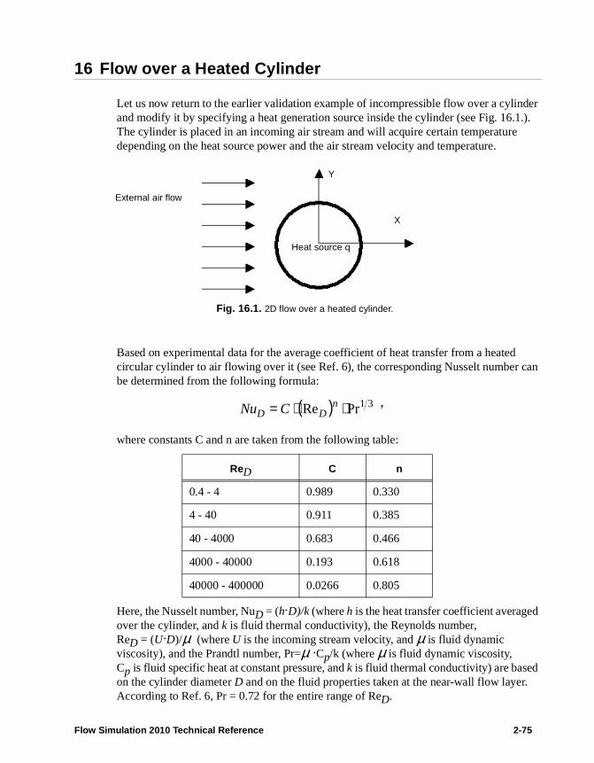
16 Flow over a Heated Cylinder
Let us now return to the earlier validation example of incompressible flow over a cylinder and modify it by specifying a heat generation source inside the cylinder (see Fig. 16.1.). The cylinder is placed in an incoming air stream and will acquire certain temperature depending on the heat source power and the air stream velocity and temperature.
Based on experimental data for the average coefficient of heat transfer from a heated circular cylinder to air flowing over it (see Ref. 6), the corresponding Nusselt number can be determined from the following formula:
where constants C and n are taken from the following table:
Here, the Nusselt number, NuD = (h·D)/k (where h is the heat transfer coefficient averaged over the cylinder, and k is fluid thermal conductivity), the Reynolds number, ReD = (U·D)/µ (where U is the incoming stream velocity, and µ is fluid dynamic viscosity), and the Prandtl number, Pr=µ ·Cp/k (where µ is fluid dynamic viscosity,
ReD C n
0.4 - 4 0.989 0.330
4 - 40 0.911 0.385
40 - 4000 0.683 0.466
4000 - 40000 0.193 0.618
40000 - 400000 0.0266 0.805
Fig. 16.1. 2D flow over a heated cylinder.
External air flow
Heat source q
Y
X
( ) 31PrRe ⋅⋅= nDD CNu ,
Flow Simulation 2010 Technical Reference 2-75
Cp is fluid specific heat at constant pressure, and k is fluid thermal conductivity) are based on the cylinder diameter D and on the fluid properties taken at the near-wall flow layer. According to Ref. 6, Pr = 0.72 for the entire range of ReD.

To validate the Flow Simulation predictions, the air properties have been specified to provide Pr = 0.72: k = 0.0251375 W/(m·K), µ = 1.8·10-5 Pa·s, specific heat at constant pressure Cp = 1005.5 J/(kg·K). Then, the incoming stream velocity, U, has been specified to obtain ReD = 1, 10, 100, 103, 104, 5·104, 105, 2·105, and 3·105 for a cylinder diameter of D = 0.1 m (see Table 16.5).
This validation approach consists of specifying the heat generation source inside the cylinder with a power determined from the desired steady-state cylinder temperature and the average heat transfer coefficient, h = (NuD·k)/D. NuD is determined from the specified ReD using the empirical formula presented above. The final cylinder surface temperature, that is also required for specifying the heat source power Q (see Table 16.5) is assumed to be 10°C higher than the incoming air temperature. The initial cylinder temperature and the incoming air temperature are equal to 293.15 K. The cylinder material is aluminum. Here, the heat conduction in the solid is calculated simultaneously with the flow calculation, i.e., the conjugate heat transfer problem is solved.
As a result of the calculation, the cylinder surface has acquired a steady-state temperature differing from the theoretical one corresponding to the heat generation source specified inside the cylinder. Multiplying the theoretical value of the Nusselt number by the ratio of the obtained temperature difference (between the incoming air temperature and the cylinder surface temperature) to the specified temperature difference, we have determined the predicted Nusselt number versus the specified Reynolds number. The values obtained by solving the steady-state and time dependent problems at result resolution level 5 are presented in Fig. 16.2. together with the experimental data taken from Ref. 6.
Table 16.5 The Flow Simulation specifications of U and Q for the problem under consideration.
From Fig. 16.2., it is seen that the predictions made with Flow Simulation, both in the time-dependent approach and in the steady-state one, are excellent within the whole ReD range under consideration.
1 1.5×10⁻⁴
0.007
10 1.5×10⁻³
0.016
102
0 .015 0.041
103
0 .15 0.121
104
1.5 0.405
105
15 1.994
R e D U , m /s Q ,W
2-76
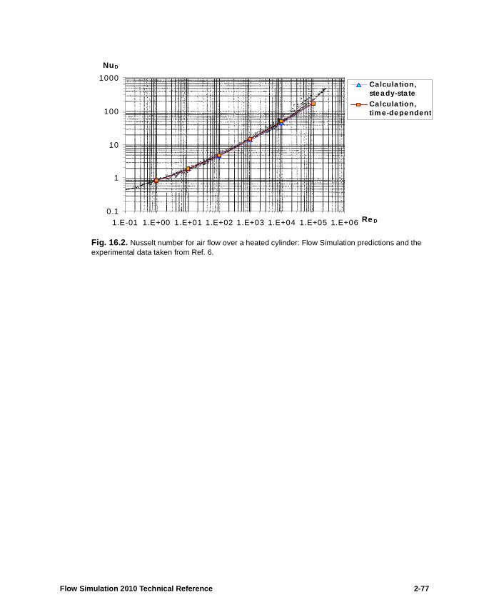
Fig. 16.2. Nusselt number for air flow over a heated cylinder: Flow Simulation predictions and the experimental data taken from Ref. 6.
0.1
1
10
100
1000
1.E-01 1.E+00 1.E+01 1.E+02 1.E+03 1.E+04 1.E+05 1.E+06 Re D
NuD
Calcula tion,steady-sta teCalcula tion,tim e-dependent
Flow Simulation 2010 Technical Reference 2-77

2-78

17 Natural Convection in a Square Cavity
Here we will consider a 2D square cavity with a steady-state natural convection, for which a highly-accurate numerical solution has been proposed in Ref.10 and used as a benchmark for about 40 computer codes in Ref.11, besides it well agrees with the semi-empirical formula proposed in Ref.12 for rectangular cavities. This cavity's configuration and imposed boundary conditions, as well as the used coordinate system, are presented in Fig. 17.1.. Here, the left and right vertical walls are held at the constant temperatures of T1 = 305 K and T2 = 295 K, accordingly, whereas the upper and bottom walls are adiabatic. The cavity is filled with air.
The square cavity's side dimension, L, is varied within the range of 0.0111...0.111 m in order to vary the cavity's Rayleigh number within the range of 103…106. Rayleigh number descibes the characteristics of the natural convection inside the cavity and is defined as follows:
,
where is the volume expansion coefficient of air,
g is the gravitational acceleration,
Cp is the air's specific heat at constant pressure,
∆T = T1 - T2 = 10 K is the temperature difference between the walls,
k is the thermal conductivity of air,
µ is the dynamic viscosity of air.
Fig. 17.1. An enclosed 2D square cavity with natural convection.
Adiabatic walls
L
T1=305 K T2=295 K
Y
g
X
µρβ
k
TLCgRa p ∆
=32
1Tβ =
Flow Simulation 2010 Technical Reference 2-79

The cavity's model is shown in Fig. 17.2..
Due to gravity and different temperatures of the cavity's vertical walls, a steady-state natural convection flow (vortex) with a vertical temperature stratification forms inside the cavity. The Ra = 105 flow's prediction performed with Flow Simulation is shown in Fig. 17.3..
Fig. 17.2. The model created for calculating the 2D natural convection flow in the 2D square cavity using Flow Simulation.
Fig. 17.3. The temperature, X-velocity, Y-velocity, the velocity vectors, and the streamlines, predicted by Flow Simulation in the square cavity at Ra = 105.
2-80

A quantitative comparison of the Flow Simulation predictions performed at result resolution level 8 with References.10, 11 (computational benchmark) and 12 (semi-empirical formula) for different Ra values is presented in Figs.17.4 - 17.6. The Nusselt number averaged over the cavity's hot vertical wall (evidently, the same value
must be obtained over the cavity's cold vertical wall) , where
qw av is the heat flux from the wall to the fluid, averaged over the wall, is considered in Fig. 17.4..
Here, the dash line presents the Ref.12 semi-empirical formula
,
where D is the distance between the vertical walls and L is the cavity height (D=L in the case under consideration). One can see that the Flow Simulation predictions practically coincide with the benchmark at Ra ≤105 and are close to the semi-empirical data.
The dimensionless velocities of the natural convection flow in the X and Y directions,
and (which are maximum along the cavity's
mid-planes, i.e., along the vertical mid-plane and along the horizontal
mid-plane) are considered in Fig. 17.5.. The dimensionless coordinates, and
, of these maximums' locations (i.e., for and for ) are
/( )av wavNu q L T k= ⋅ ∆ ⋅
1/ 4 1/ 40.28 ( / )avNu Ra L D −= ⋅
Fig. 17.4. The average sidewall Nusselt number vs. the Rayleigh number.
0
1
2
3
4
5
6
7
8
9
10
1.E+03 1.E+04 1.E+05 1.E+06Ra
Nuav
Refs.10, 11Ref.12
Calculation
pU L CU
k
ρ⋅ ⋅ ⋅= pV L C
Vk
ρ⋅ ⋅ ⋅=
maxU maxV
L
xx =
yy = y maxU x maxV
Flow Simulation 2010 Technical Reference 2-81
presented in Fig. 17.6.. One can see that the Flow Simulation predictions of the natural
convection flow's local parameters are fairly close to the benchmark data at Ra ≤105.
L

Fig. 17.5. Dimensionless maximum velocities vs. Rayleigh number.
1
10
100
1000
1.E+03 1.E+04 1.E+05 1.E+06 Ra
Dim
ensi
on
less
U
max
, V
max
Vmax, Refs.10, 11
Vmax, calculation
Umax, Refs.10, 11
Umax, calculation
Fig. 17.6. Dimensionless coordinates of the maximum velocities' locations.
0
0.1
0.2
0.3
0.4
0.5
0.6
0.7
0.8
0.9
1
1.E+03 1.E+04 1.E+05 1.E+06 Ra
Dim
ensi
on
less
X V
max
, Y
Um
ax
Y Umax, Refs.10, 11
Y Umax, calculation
X Vmax, Refs.10, 11
X V max,calculation
2-82

18 Particles Trajectories in Uniform Flows
Let us now consider the Flow Simulation capability to predict particles trajectories in a gas flow (i.e. two-phase flow of fluid + liquid droplets or solid particles).
In accordance with the particles motion model accepted in Flow Simulation, particle trajectories are calculated after completing a fluid flow calculation (which can be either steady or time-dependent). That is, the particles mass and volume flow rates are assumed substantially lower than those of the fluid stream, so that the influence of particles’ motions and temperatures on the fluid flow parameters is negligible, and motion of the particles obeys the following equation:
where m is the particle mass, t is time, Vp and Vf are the particle and fluid velocities (vectors), accordingly, ρf is the fluid density, Cd is the particle drag coefficient, A is the particle frontal surface area, and Fg is the gravitational force.
Particles are treated as non-rotating spheres of constant mass and specified (solid or liquid) material, whose drag coefficient is determined from Henderson’s semi-empirical formula (Ref. 18). At very low velocity of particles with respect to carrier fluid (i.e., at the relative velocity’s Mach number M → 0) this formula becomes
where Reynolds number is defined as
d is the diameter of particles, and µ is the fluid dynamic viscosity.
To validate Flow Simulation, let us consider three cases of injecting a particle perpendicularly into an incoming uniform flow, Fig. 18.1.. Since both the fluid flow and the particle motion in these cases are 2D (planar), we will solve a 2D (i.e. in the XY-plane) flow problem.
gd
pfpffp FACVVVV
dt
dVm +
−⋅−−=
2
)(ρ ,
380.Re480Re0301
124.
Re
24Cd +
+⋅++=
..
µρ dVV pff −
=Re ,
Uniform fluid flow
Particle injection
Flow Simulation 2010 Technical Reference 2-83
Fig. 18.1. Injection of a particle into a uniform fluid flow.

Due to the same reason as in the previous validation examples with flow over flat plates, we will solve this validation as an internal problem. The corresponding SolidWorks model is shown in Fig. 18.2.. Both of the walls are ideal, the channel has length of 0.233 m and height of 0.12 m, all the walls have thickness of 0.01 m. We specify the uniform fluid velocity Vinlet, the fluid temperature of 293.2 K, and the default values of turbulent flow parameters with the laminar boundary layer at the channel inlet, and the static pressure of 1 atm at the channel outlet. All the fluid flow calculations are performed at a result resolution level of 5.
To validate calculations of particles trajectories by comparing them with available analytical solutions of the particle motion equation, we consider the following three cases:
a) the low maximum Reynolds number of Re max = 0.1 (air flow with Vinlet = 0.002 m/s, gold particles of d = 0.5 mm, injected at the velocity of 0.002 m/s perpendicularly to the wall),
b) the high maximum Reynolds number of Re max = 105 (water flow with Vinlet = 10 m/s, iron particles of d = 1 cm, injected at the velocities of 1, 2, 3 m/s perpendicularly to the wall),
c) a particle trajectory in the Y-directed gravitational field (gravitational acceleration gy = -9.8 m/s2, air flow with Vinlet = 0.6 m/s, an iron particle of d = 1 cm, injected at the 1.34 m/s velocity at the angle of 63.44o with the wall).
In the first case, due to small Re values, the particle drag coefficient is close to Cd=24/Re (i.e., obeys the Stokes law). Then, neglecting gravity, we obtain the following analytical solution for the particle trajectory:
Fig. 18.2. The model.
Inlet
Outlet
Ideal Wall
Origin and particle injection point
)18
exp()(18
)(20
2
0t
dVV
dtVXtX
pfxtpx
pfxt ρ
µµρ
−⋅−+⋅+===
,
182d p µρ ,
2-84
)exp()(18
)( 200t
dVVtVYtY
pfytpyfyt ρµ
−⋅−+⋅+===

where Vfx, Vpx, Vfy, Vpy are the X- and Y-components of the fluid and particle velocities, accordingly, ρp is the particle material density. The Flow Simulation calculation and the analytical solution are shown in Fig. 18.3.. It is seen that they are very close to one another. Special calculations have shown that the difference is due to the CD assumptions only.
In the second case, due to high Re values, the particle drag coefficient is close to Cd=0.38. Then, neglecting the gravity, we obtain the following analytical solution for the particle trajectory:
The Flow Simulation calculations and the analytical solutions for three particle injection velocities, Vpy(t=0) = 1, 2, 3 m/s, are shown in Fig. 18.4.. It is seen that the Flow Simulation calculations coincide with the analytical solutions. Special calculations have shown that the difference is due to the CD assumptions only.
In the third case, the particle trajectory is governed by the action of the gravitational force only, the particle drag coefficient is very close to zero, so the analytical solution is:
Fig. 18.3. Particle trajectories in a uniform fluid flow at Re max = 0.1, predicted by Flow Simulation and obtained from the analytical solution.
0.000
0.005
0.010
0.015
0.020
0.025
0.030
0.035
0.00 0.05 0.10 0.15 0.20 0.25 X (m)
Y (m)
AnalyticalsolutionCalculation
)285.0
1ln()(285.0
)(00
td
VVd
tVYtYp
fytpyp
fyt ρρ
ρρ
+⋅−+⋅+===
,
).
ln()(.
)( td
28501VV
2850
dtVXtX
pfx0tpx
pfx0t ρ
ρρ
ρ+⋅−+⋅+=
==.
2
Flow Simulation 2010 Technical Reference 2-85
0
00 2
1
−⋅++= =
==px
ttpyt V
XXy
gtVYY .

The Flow Simulation calculation and the analytical solution for this case are presented in Fig. 18.5.. It is seen that the Flow Simulation calculation coincides with the analytical solution.
I
Fig. 18.4. Particle trajectories in a uniform fluid flow at Re max = 105, predicted by Flow Simulation and obtained from the analytical solution.
0.00
0.01
0.02
0.03
0.04
0.05
0.06
0.07
0.08
0.00 0.05 0.10 0.15 0.20 X (m)
Y (m)
Vp = 1 m/s,analytical solution
Vp = 1 m/s,Calculation
Vp = 2 m/s,analytical solution
Vp = 2 m/s,Calculation
Vp = 3 m/s,analytical solution
Vp = 3 m/s,Calculation
Fig. 18.5. Particle trajectories in the Y-directed gravity, predicted by Flow Simulation and obtained from the analytical solution.
0
0.01
0.02
0.03
0.04
0.05
0.06
0.07
0.08
0.00 0.03 0.06 0.09 0.12 0.15 X (m)
Y (m)
Calculation
Theory
2-86

19 Porous Screen in a Non-uniform Stream
Let us now validate the Flow Simulation capability to calculate fluid flows through porous media.
Here, following Ref. 2, we consider a plane cold air flow between two parallel plates, through a porous screen installed between them, see Fig. 19.1.. At the channel inlet the air stream velocity profile is step-shaped (specified). The porous screen (gauze) levels this profile to a more uniform profile. This effect depends on the screen drag, see Ref. 2.
The SolidWorks model used for calculating the 2D (in XY-plane) flow is shown in Fig. 19.2.. The channel has height of 0.15 m, the inlet (upstream of the porous screen) part of the 0.3 m length, the porous screen of the 0.01 m thickness, and the outlet (downstream of the porous screen) part of the 0.35 m length. All the walls have thickness of 0.01 m.
Air
L
Porous screen
X
Y
Fig. 19.1. Leveling effect of a porous screen (gauze) on a non-uniform stream.
Fig. 19.2. The SolidWorks model used for calculating the 2D flow between two parallel plates and through the porous screen with Flow Simulation.
Flow Simulation 2010 Technical Reference 2-87
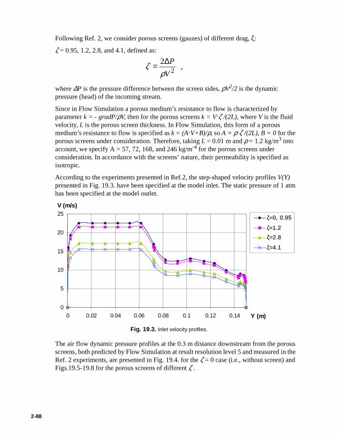
Following Ref. 2, we consider porous screens (gauzes) of different drag, ζ:
ζ = 0.95, 1.2, 2.8, and 4.1, defined as:
where ∆P is the pressure difference between the screen sides, ρV2/2 is the dynamic pressure (head) of the incoming stream.
Since in Flow Simulation a porous medium’s resistance to flow is characterized by parameter k = - gradP/ρV, then for the porous screens k = V·ζ /(2L), where V is the fluid velocity, L is the porous screen thickness. In Flow Simulation, this form of a porous medium’s resistance to flow is specified as k = (A·V+B)/ρ, so A = ρ·ζ /(2L), B = 0 for the porous screens under consideration. Therefore, taking L = 0.01 m and ρ = 1.2 kg/m3 into account, we specify A = 57, 72, 168, and 246 kg/m-4 for the porous screens under consideration. In accordance with the screens’ nature, their permeability is specified as isotropic.
According to the experiments presented in Ref.2, the step-shaped velocity profiles V(Y) presented in Fig. 19.3. have been specified at the model inlet. The static pressure of 1 atm has been specified at the model outlet.
The air flow dynamic pressure profiles at the 0.3 m distance downstream from the porous screens, both predicted by Flow Simulation at result resolution level 5 and measured in the Ref. 2 experiments, are presented in Fig. 19.4. for the ζ = 0 case (i.e., without screen) and Figs.19.5-19.8 for the porous screens of different ζ .
22
V
P
ρζ ∆= ,
Fig. 19.3. Inlet velocity profiles.
0
5
10
15
20
25
0 0.02 0.04 0.06 0.08 0.1 0.12 0.14 Y (m)
V (m/s)
ζ=0, 0.95
ζ=1.2
ζ=2.8
ζ=4.1
2-88
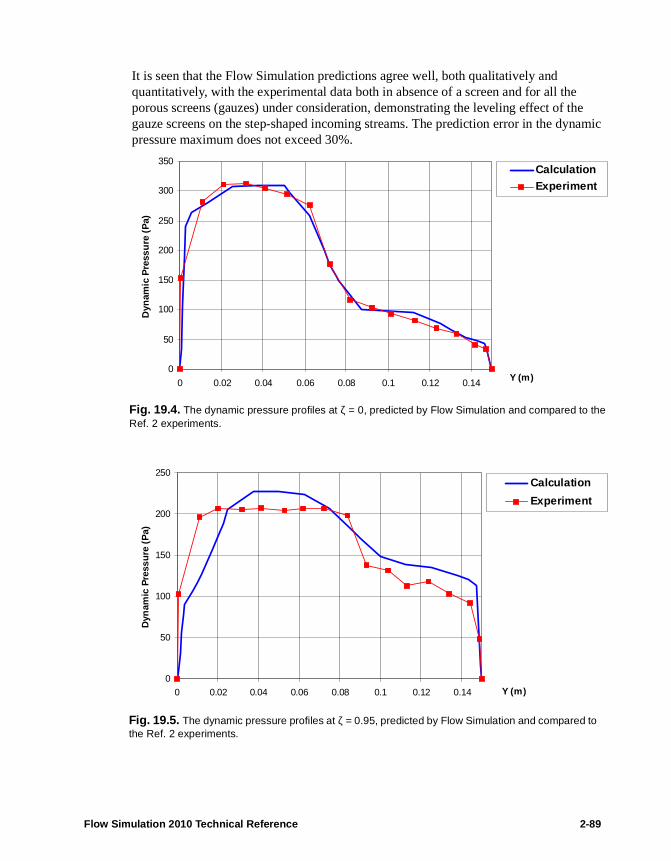
It is seen that the Flow Simulation predictions agree well, both qualitatively and quantitatively, with the experimental data both in absence of a screen and for all the porous screens (gauzes) under consideration, demonstrating the leveling effect of the gauze screens on the step-shaped incoming streams. The prediction error in the dynamic pressure maximum does not exceed 30%.
Fig. 19.4. The dynamic pressure profiles at ζ = 0, predicted by Flow Simulation and compared to the Ref. 2 experiments.
0
50
100
150
200
250
300
350
0 0.02 0.04 0.06 0.08 0.1 0.12 0.14 Y (m)
Dyn
amic
Pre
ssu
re (
Pa)
CalculationExperiment
Fig. 19.5. The dynamic pressure profiles at ζ = 0.95, predicted by Flow Simulation and compared to the Ref. 2 experiments.
0
50
100
150
200
250
0 0.02 0.04 0.06 0.08 0.1 0.12 0.14 Y (m)
Dyn
amic
Pre
ssu
re (
Pa)
Calculation
Experiment
Flow Simulation 2010 Technical Reference 2-89
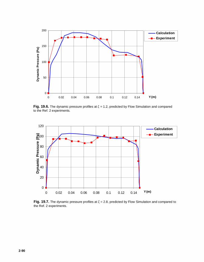
Fig. 19.6. The dynamic pressure profiles at ζ = 1.2, predicted by Flow Simulation and compared to the Ref. 2 experiments.
0
50
100
150
200
0 0.02 0.04 0.06 0.08 0.1 0.12 0.14 Y (m)
Dyn
amic
Pre
ssur
e (P
a)Calculation
Experiment
Fig. 19.7. The dynamic pressure profiles at ζ = 2.8, predicted by Flow Simulation and compared to the Ref. 2 experiments.
0
20
40
60
80
100
120
0 0.02 0.04 0.06 0.08 0.1 0.12 0.14 Y (m)
Dyn
amic
Pre
ssu
re (
Pa)
Calculation
Experiment
2-90

Fig. 19.8. The dynamic pressure profiles at ζ = 4.1, predicted by Flow Simulation and compared to the Ref. 2 experiments.
0
10
20
30
40
50
60
70
80
90
0 0.02 0.04 0.06 0.08 0.1 0.12 0.14 Y (m)
Dyn
amic
Pre
ssu
re (
Pa)
Calculation
Experiment
Flow Simulation 2010 Technical Reference 2-91

2-92

20 Lid-driven Flows in Triangular and Trapezoidal Cavities
Let us now see how Flow Simulation predicts lid-driven (i.e., shear-driven) 2D recirculating flows in closed 2D triangular and trapezoidal cavities with one or two moving walls (lids) in comparison with the calculations performed in Ref. 21 and Ref. 20.
These two cavities are shown in Fig. 20.1.. The triangular cavity has a moving top wall, the trapezoidal cavity has a moving top wall also, whereas its bottom wall is considered in two versions: as motionless and as moving at the top wall velocity. The no-slip conditions are specified on all the walls.
As shown in Ref. 21 and Ref. 20, the shear-driven recirculating flows in these cavities are fully governed by their Reynolds numbers Re = ρ·Uwall·h/µ, where ρ is the fluid density, µ is the fluid dynamic viscosity, Uwall is the moving wall velocity, h is the cavity height. So, we can specify the height of the triangular cavity h = 4 m, the height of the trapezoidal cavity h = 1 m, Uwall = 1 m/s for all cases under consideration, the fluid density ρ = 1 kg/m3, the fluid dynamic viscosity µ=0.005 Pa·s in the triangular cavity produces a Re = 800, and µ= 0.01, 0.0025, 0.001 Pa·s in the trapezoidal cavity produces a Re = 100, 400, 1000, respectively.
Fig. 20.1. The 2D triangular (left) and trapezoidal (right) cavities with the moving walls (the motionless walls are shown with dashes).
2
h
U
1
1
2
U
U
Uwa
Flow Simulation 2010 Technical Reference 2-93

The cavities’ models are shown in Fig. 20.2.. The Flow Simulation calculation of flow in the triangular cavity has been performed on the 48x96 computational mesh. The results in comparison with those from Ref. 21 are presented in Fig. 20.3. (streamlines) and in Fig. 20.4. (the fluid velocity X-component along the central vertical bisector shown by a green line in Fig. 20.2.). A good agreement of these calculations is clearly seen.
Fig. 20.2. The models for calculating the lid-driven 2D flows in the triangular (left) and trapezoidal (right) cavities with Flow Simulation.
Fig. 20.3. The flow trajectories in the triangular cavity, calculated by Flow Simulation (right) and compared to the Ref. 21 calculation (left).
2-94

The Flow Simulation calculations of flows in the trapezoidal cavity with one and two moving walls at different Re values have been performed with the 100x50 computational mesh. Their results in comparison with those from Ref.16 are presented in Fig. 20.5.-20.10 (streamlines) and in Fig. 20.11. (the fluid velocity X-component along the central vertical bisector shown by a green line in Fig. 20.2.). A good agreement of these calculations is seen.
Fig. 20.5. The flow streamlines in the trapezoidal cavity with a top only moving wall at Re = 100, calculated by Flow Simulation (right) and compared to the Ref. 20 calculation (left).
Fig. 20.4. The triangular cavity’s flow velocity X-component along the central vertical bisector, calculated by Flow Simulation (red line) and compared to the Ref. 21 calculation (black line with circlets).
-0.4
-0.2
0
0.2
0.4
0.6
0.8
1
1.2
0 0.5 1 1.5 2 2.5 3 3.5 4
Y, m
Vx/Uwall
Calculation
Flow Simulation 2010 Technical Reference 2-95

Fig. 20.6. The flow streamlines in the trapezoidal cavity with a top only moving wall at Re = 400, calculated by Flow Simulation (right) and compared to the Ref. 20 calculation (left).
Fig. 20.7. The flow streamlines in the trapezoidal cavity with a top only moving wall at Re = 1000, calculated by Flow Simulation (right) and compared to the Ref. 20 calculation (left).
Fig. 20.8. The flow streamlines in the trapezoidal cavity with two moving walls at Re = 100, calculated by Flow Simulation (right) and compared to the Ref. 20 calculation (left).
2-96

Fig. 20.9. The flow streamlines in the trapezoidal cavity with two moving walls at Re = 400, calculated by Flow Simulation (right) and compared to the Ref. 20 calculation (left).
Fig. 20.10. The flow streamlines in the trapezoidal cavity with two moving walls at Re = 1000, calculated by Flow Simulation (right) and compared to the Ref. 20 calculation (left).
Fig. 20.11. The flow velocity X-component along the central vertical bisector in the trapezoidal cavity with two moving walls at Re = 400, calculated by Flow Simulation (red line) and compared to the Ref. 20 calculation (black line).
-1
-0.8
-0.6
-0.4
-0.2
0
0.2
0.4
0.6
0.8
1
0 0.2 0.4 0.6 0.8 1
Y, m
Vx/Uwall
Calculation
Flow Simulation 2010 Technical Reference 2-97

2-98

21 Flow in a Cylindrical Vessel with a Rotating Cover
Let us now see how Flow Simulation predicts a 3D recirculating flow in a cylindrical vessel closed by a rotating cover (see Fig. 21.1.) in comparison with the experimental data presented in Ref. 21 (also in Ref. 22). This vessel of R = h = 0.144 m dimensions is filled with a glycerol/water mixture. The upper cover rotates at the angular velocity of Ω. The other walls of this cavity are motionless. The default no-slip boundary condition is specified for all walls.
Due to the cover rotation, a shear-driven recirculating flow forms in this vessel. Such flows are governed by the Reynolds number Re = ρ·Ω·R2/µ, where ρ is the fluid density, µ is the fluid dynamic viscosity, Ω is the angular velocity of the rotating cover, R is the radius of the rotating cover. In the case under consideration the 70/30% glycerol/water mixture has ρ = 1180 kg/m3, µ = 0.02208 Pa·s, the cover rotates at Ω = 15.51 rpm, so Re = 1800.
The Flow Simulation calculation has been performed on the 82x41x82 computational mesh. The formed flow pattern (toroidal vortex) obtained in this calculation is shown in Fig. 21.2. using the flow velocity vectors projected onto the XY-plane. The tangential and radial components of the calculated flow velocity along four vertical lines arranged in the XY-plane at different distances from the vessel axis in comparison with the Ref. 21 experimental data are presented in Figs.21.3-7 in the dimensionless form (the Y-coordinate is divided by R, the velocity components are divided by Ω·R). There is good agreement with the calculation results and the experimental data shown.
Fig. 21.1. The cylindrical vessel with the a rotating cover.
rotating coverΩ
R
h
Flow Simulation 2010 Technical Reference 2-99

Fig. 21.2. The vessel's flow velocity vectors projected on the
Fig. 21.3. The vessel's flow tangential and radial velocity components along the X = 0.6 vertical, calculated by Flow Simulation (red) and compared to the Ref. 21 experimental data.
2-100

Fig. 21.4. The vessel's flow tangential and radial velocity components along the X = 0.7 vertical, calculated by Flow Simulation (red) and compared to the Ref. 21 experimental data.
Fig. 21.5. The vessel's flow tangential and radial velocity components along the X = 0.8 vertical, calculated by Flow Simulation (red) and compared to the Ref. 21 experimental data.
Flow Simulation 2010 Technical Reference 2-101

Fig. 21.6. The vessel's flow tangential and radial velocity components along the X = 0.9 vertical, calculated by Flow Simulation (red) and compared to the Ref. 21 experimental data.
2-102

22 Flow in an Impeller
Let us now validate the Flow Simulation ability to perform calculations in a rotating coordinate system related to a rotating solid. Following Ref. 23, we will consider the flow of water in a 9-bladed centrifugal impeller having blades tilted at a constant 60° angle with respect to the intersecting radii and extending out from the 320 mm inner diameter to the 800 mm outer diameter (see Fig. 22.1.). The water in this impeller flows from its center to its periphery. To compare the calculation with the experimental data presented in Ref.22, the impeller's angular velocity of 32 rpm and volume flow rate of 0.00926 m3/s are specified.
Since the impeller's inlet geometry and disk extension serving as the impeller's vaneless diffuser have no exact descriptions in Ref. 23, to perform the validating calculation we arbitrarily specified the annular inlet as 80 mm in diameter with an uniform inlet velocity profile perpendicular to the surface in the stationary coordinate system.The impeller's disks external end was specified as 1.2 m diameter, as shown in Fig. 22.2..
The above-mentioned volume flow rate at the annular inlet and the potential pressure of 1 atm at the annular outlet are specified as the problem's flow boundary conditions.
Fig. 22.1. The impeller's blades geometry.
Fig. 22.2. The model used for calculating the 3D flow in the impeller.
Flow Simulation 2010 Technical Reference 2-103

The Flow Simulation 3D flow calculation is performed on the computational mesh using the result resolution level of 5 and the minimum wall thickness of 2 mm (since the blades have constant thickness). To further capture the curvature of the blades a local initial mesh was also used in the area from the annular inlet to the blades' periphery. As a result, the computational mesh has a total number of about 1,000,000 cells.
Following Ref. 23, let us compare the passage-wise flow velocities (ws, see their definition in Fig. 22.3., β = 60°) along several radial lines passing through the channels between the blades (lines g, j, m, p in Fig. 22.4.) at the mid-height between the impeller's disks.
The passage-wise flow velocities divided by Ωxr2, where Ω is the impeller's angular velocity and r2 = 400 mm is the impeller's outer radius, which were measured in Ref. 23 and obtained in the performed Flow Simulation calculations, are shown in Fig. 22.5., 6, 7, and 8. In these figures, the distance along the radial lines is divided by the line's length. The Flow Simulation results are presented in each of these figures by the curve obtained by averaging the corresponding nine curves in all the nine flow passages between the impeller blades. The calculated passage-wise flow velocity's cut plot covering the whole
Fig. 22.3. Definition of the passage-wise flow velocity.
Fig. 22.4. Definition of the reference radial lines along which the passage-wise flow velocity was measured in Ref. 23 (from a to s in the alphabetical order).
2-104
computational domain at the mid-height between the impeller's disks is shown in Fig. 22.9.. Here, the g, j, m, p radial lines in each of the impeller's flow passages are shown. A good agreement of these calculation results with the experimental data is seen.

Fig. 22.5. The impeller's passage-wise flow velocity along the g (see Fig. 22.4.) radial line, calculated by Flow Simulation and compared to the experimental data.
0
0 .25
0 .5
0 .75
0 0 .2 0 .4 0 .6 0 .8 1
re lative d is tance along the rad ial line
rela
tive
pas
sag
ewis
e ve
loci
ty
(ave
rag
ed)
calculation
exp eriment
Fig. 22.6. The impeller's passage-wise flow velocity along the j (see Fig. 22.4.) radial line, calculated by Flow Simulation and compared to the experimental data.
0
0 .25
0.5
0 .75
0 0.2 0.4 0 .6 0 .8 1
relative distance along the radial line
rela
tive
pas
sag
ewis
e ve
loci
ty
(ave
rag
ed)
calculation
experiment
Flow Simulation 2010 Technical Reference 2-105

Fig. 22.7. The impeller's passage-wise flow velocity along the m (see Fig. 22.4.) radial line, calculated by Flow Simulation and compared to the experimental data.
0
0 .2 5
0 .5
0 .7 5
0 0 .5 1
re lative d is tanc e a lo ng the rad ia l line
rela
tive
pass
agew
ise
velo
city
(ave
rage
d)c a lc u la tio n
e x p e rim e n t
Fig. 22.8. The impeller's passage-wise flow velocity along the p (see Fig. 22.4.) radial line, calculated by Flow Simulation and compared to the experimental data.
0
0.2 5
0 .5
0.7 5
0 0.2 0 .4 0.6 0 .8 1
re lative d is tance alo ng the rad ial line
rela
tive
pa
ssag
ewis
e v
elo
city
(ave
rage
d)
calculatio n
experim en t
2-106

Fig. 22.9. A cut plot of the impeller's passage-wise flow velocity calculated by Flow Simulation.
Flow Simulation 2010 Technical Reference 2-107

2-108

23 Cavitation on a hydrofoil
When the local pressure at some point in the liquid drops below the liquid's vapour pressure at the local temperature, the liquid undergoes phase transition and form cavities filled with the liquid's vapor with an addition of gas that has been dissolved in the liquid. This phenomenon is called cavitation.
In this validation example we consider Flow Simulation abilities to model cavitation on the example of water flow around a symmetric hydrofoil in a water-filled tunnel. The calculated results were compared with the experimental data from Ref. 24.
The problem is solved in the 2D setting. A symmetric hydrofoil with the chord c of 0.305 m is placed in a water-filled tunnel with the angle of attack of 3.5°. The part of the tunnel being modelled has the following dimensions: length l = 2 m and height h = 0.508 m. The calculation is performed four times with different values of the cavitation number σ defined as follows:
where P∞ is the inlet pressure, Pv is the saturated water vapor pressure equal to 2340 Pa at given temperature (293.2 K), ρ is the water density at inlet, and U∞ is the water velocity at inlet (see Fig. 23.1.).
The inlet boundary condition is set up as Inlet Velocity of 8 m/s. On the tunnel outlet an Environment Pressure is specified so that by varying it one may tune the cavitation number to the needed value. The project fluid is water with the cavitation option switched on, while the other parameters are default. A local initial mesh was created in order to resolve the cavitation area better. The resulting mesh contains about 30000 cells.
2
21
∞
∞ −=U
PP v
ρσ
Fig. 23.1. The model geometry.
Flow Simulation 2010 Technical Reference 2-109

The qualitative comparison in a form of cut plots with Vapor Volume Fraction as the visualization parameter are shown on Fig. 23.2.
Fig. 23.2. A comparison of calculated and experimentally observed cavitation areas for different σ
σ=1.1 σ=0.97
σ=0.9 σ=0.88
2-110

The calculated length of the cavitation area was derived from the distribution of the Vapor Volume Fraction parameter over the hydrofoil’s surface as the distribution’s width at half-height. The results are presented on Fig. 23.3.
According to Ref. 24, the "clear appearance" of the cavity becomes worse for larger cavity lengths. The experimental data also confirm that the amount of uncertainty increases with increasing cavity extent. Taking these factors into account together with the comparison performed above, we can see that the calculated length of the cavitation area agrees well with the experiment for a wide range of cavitation numbers.
Pressure measurements were performed on the hydrofoil surface at x/c = 0.05 in order to calculate the pressure coefficient defined as follows:
A comparison of the calculated and experimental values of this parameter is presented on Fig. 23.4. and also shows a good agreement.
Fig. 23.3. A comparison of calculated and measured cavitation lengths
2
05.0/
2
1∞
=∞ −=−U
PPC cx
p
ρ
Flow Simulation 2010 Technical Reference 2-111

Fig. 23.4. A comparison of calculated and measured pressure coefficient
2-112

24 Isothermal Cavitation in a Throttle Nozzle
In this validation example we consider Flow Simulation capabilities to simulate cavitation in industrial liquid flows using the Isothermal cavitation model. The problem studied here validates this model by considering a 3D diesel fuel flow in a throttle channel that was studied experimentally in Ref. 25. According to this work, thermal effects in the considered flow are negligible. Therefore, it is reasonable to apply the Isothermal cavitation model.
Throttle channel geometry with its main dimensions is shown in Fig. 24.1
Diesel fuel at 30°C is supplied to the inlet under the pressure (Pin) of 100 bar. The outlet pressure (Pout) varies from 10 to 70 bar. The properties of the analyzed fuel for the given temperature are presented in Table 24.1.
Table 24.1 Properties of the diesel fuel (2-D) at 30°C.
It is assumed that fuel contains dissolved air. The mass fraction of dissolved air is set to 0.001 to conform with the experimental data.
Fig. 24.1 The channel geometry: L=1mm, H=0.299mm, W=0.3mm, Rin=0.02mm.
Density (kg/m3) 836
Molar Mass (kg/mol) 0.198
Dynamic Viscosity (Pa*s) 0.0025
Saturation Pressure (Pa) 2000
Flow Simulation 2010 Technical Reference 2-113

The objective of the calculations is to obtain channel characteristic under cavitation conditions and compare it with the experimental measurements. Because throttle channel has a symmetry plane, only a half of the model is used to generate the computational mesh. A finer local mesh is used to resolve the flow in the narrow channel and the adjacent regions providing about 15 mesh cells across the channel half-height. Additional refinement is performed in the region near the small fillet Rin. The resulting mesh are shown in Fig. 24.2.
Fig. 24.3 shows the distribution of the vapour volume fraction at different pressure drop. This figure provides a view of the initiation and development of the cavitation area.
Fig. 24.2 The computational mesh (zoom-view).
Fig. 24.3 Cavitation fields at symmetry plane.
∆P = 67 bar ∆P = 75 bar ∆P = 90 bar
2-114

The dependency of the pressure drop on the mass flow rate both predicted by Flow Simulation and determined experimentally are shown on Fig. 24.4. The difference between the calculations and the experimental measurements is less than 5%. Also, as it can be seen from the Fig. 24.3 and Fig. 24.4, the critical cavitation point corresponds to the pressure drop of about 70 bar. This point defines the transition from a pressure-dependent mass flow to choked mass flow that is induced by cavitation.
The comparison of the Flow Simulation calculations with the experimental data shows that the application of the Isothermal cavitation model that employs a limited set of fluid properties allows to predict cavitating flow characteristics with the sufficient accuracy.
Fig. 24.4 Mass flow rate versus pressure drop at 100 bar inlet pressure in comparison with the experimental data (Ref. 25).
0.004
0.005
0.006
0.007
0.008
0.009
20 30 40 50 60 70 80 90 100
∆P, bar
G, kg/s
Experiment
Calculation
Flow Simulation 2010 Technical Reference 2-115

2-116

25 Thermoelectric Cooling
Flow Simulation has the ability to model the work of a thermoelectric cooler (TEC), also known as Peltier element. The device used in this example has been developed for active cooling of an infrared focal plane array detector used during the Mars space mission (see Ref. 26).
According to the hardware requirements, the cooler (see Fig. 25.1.) has the following dimensions: thickness of 4.8 mm, cold side of 8x8 mm2 and hot side of 12X12 mm2. It was built up of three layers of semiconductor pellets made of (Bi,Sb)2(Se,Te)3-based material. The cooler was designed to work at temperatures of hot surface in the range of 120-180 K and to provide the temperature drop of more than 30 K between its surfaces.
To solve the engineering problem using Flow Simulation, the cooler has been modelled by a truncated pyramidal body with fixed temperature (Temperature boundary condition) on the hot surface and given heat flow (Heat flow boundary condition) on the cold surface (see Fig. 25.3.).
Fig. 25.1. Structure of the thermoelectric cooler. Fig. 25.2. The thermoelectric module test setup. (Image from Ref. 26)
Flow Simulation 2010 Technical Reference 2-117
Fig. 25.3. The model geometry.
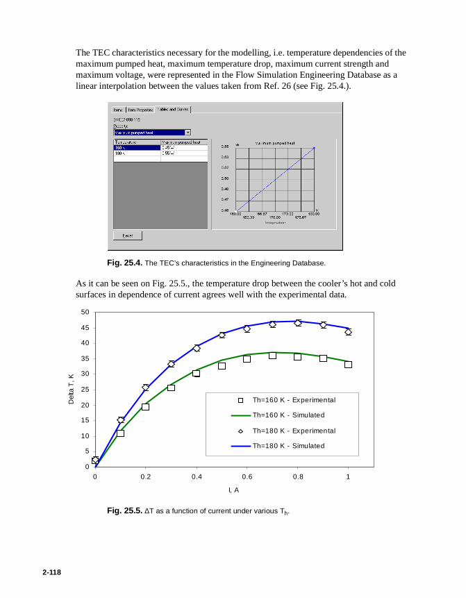
The TEC characteristics necessary for the modelling, i.e. temperature dependencies of the maximum pumped heat, maximum temperature drop, maximum current strength and maximum voltage, were represented in the Flow Simulation Engineering Database as a linear interpolation between the values taken from Ref. 26 (see Fig. 25.4.).
As it can be seen on Fig. 25.5., the temperature drop between the cooler’s hot and cold surfaces in dependence of current agrees well with the experimental data.
Fig. 25.4. The TEC’s characteristics in the Engineering Database.
Fig. 25.5. ∆T as a function of current under various Th.
0
5
10
15
20
25
30
35
40
45
50
0 0.2 0.4 0.6 0.8 1
I, A
Del
ta T
, K
Th=160 K - Experimental
Th=160 K - Simulated
Th=180 K - Experimental
Th=180 K - Simulated
2-118

The dependency of ∆T against heat flow under various Th (see Fig. 25.6.) is also in a good agreement with the performance data, as well as the coefficient of performance COP (see Fig. 25.7.) defined as follows:
where Pin is the cooler’s power consumption, and Qc and Qh are the heat flows on the cold and hot faces, respectively.
COPQc
Pin-------
Qc
Qh Qc–-------------------= =
Fig. 25.6. ∆T as a function of heat flow under various Th.
0
5
10
15
20
25
30
35
40
45
50
0.0 0.1 0.2 0.3 0.4 0.5 0.6
Qc, W
Del
ta T
, K
Th=160 K - Perf ormance Curve
Th=160 K - Simulation
Th=180 K - Perf ormance Curve
Th=180 K - Simulation
Flow Simulation 2010 Technical Reference 2-119

Finally, we may conclude that Flow Simulation reproduces thermal characteristics of the thermoelectric coolers at various currents and temperatures with good precision.
Fig. 25.7. COP as a function of ∆T under various Th.
0.00
0.02
0.04
0.06
0.08
0.10
0.12
0.14
0.16
0.0 10.0 20.0 30.0 40.0 50.0
Delta T, K
CO
P
Th=160 K - Performance Curve
Th=160 K - Simulation
Th=180 K - Performance Curve
Th=180 K - Simulation
2-120

References
1 Schlichting, H., Boundary Layer Theory. 7th ed., McGraw –Hill, New York, 1979.
2 Idelchik, I.E., Handbook of Hydraulic Resistance. 2nd ed., Hemisphere, New York, 1986.
3 Panton, R.L., Incompressible Flow. 2nd ed., John Wiley & Sons, Inc., 1996.
4 White, F.M., Fluid Mechanics. 3rd ed., McGraw-Hill, New York, 1994.
5 Artonkin, V.G., Petrov, K.P., Investigations of aerodynamic characteristics of segmental conic bodies. TsAGI Proceedings, No. 1361, Moscow, 1971 (in Russian).
6 Holman, J.P., Heat Transfer. 8th ed., McGraw-Hill, New York, 1997.
7 Humphrey, J.A.C., Taylor, A.M.K., and Whitelaw, J.H., Laminar Flow in a Square Duct of Strong Curvature. J. Fluid Mech., v.83, part 3, pp.509-527, 1977.
8 Van Dyke, Milton, An Album of Fluid Motion. The Parabolic press, Stanford, California, 1982.
9 Davis, G. De Vahl: Natural Convection of Air in a Square Cavity: a Bench Mark Numerical Solution. Int. J. for Num. Meth. in Fluids, v.3, pp. 249-264 (1983).
10 Davis, G. De Vahl, and Jones, I.P.: Natural Convection in a Square Cavity: a Comparison Exercise. Int. J. for Num. Meth. in Fluids, v.3, pp. 227-248 (1983).
11 Emery, A., and Chu, T.Y.: Heat Transfer across Vertical Layers. J. Heat Transfer, v. 87, p. 110 (1965).
12 Denham, M.K., and Patrick, M.A.: Laminar Flow over a Downstream-Facing Step in a Two-Dimensional Flow Channel. Trans. Instn. Chem. Engrs., v.52, pp. 361-367 (1974).
13 Yanshin, B.I.: Hydrodynamic Characteristics of Pipeline Valves and Elements. Convergent Sections, Divergent Sections, and Valves. “Mashinostroenie”, Moscow, 1965.
14 Enchao Yu, Yogendra Joshi: Heat Transfer Enhancement from Enclosed Discrete Components Using Pin-Fin Heat Sinks. Int. J. of Heat and Mass Transfer, v.45, p.p. 4957-4966 (2002).
15 Kuchling, H., Physik, VEB FachbuchVerlag, Leipzig, 1980.
16 Balakin, V., Churbanov, A., Gavriliouk, V., Makarov, M., and Pavlov, A.: Verification and Validation of EFD.Lab Code for Predicting Heat and Fluid Flow, In: CD-ROM Proc. Int. Symp. on Advances in Computational Heat Transfer “CHT-04”, April 19-24, 2004, Norway, 21 p.
17 Jonsson, H., Palm B., Thermal and Hydraulic Behavior of Plate Fin and Strip Fin Heat Sinks Under Varying Bypass Conditions, Proc. 1998 Intersociety Conf. On Thermal and Thermomechanical Phenomena in Electronic Systems (ITherm ’98), Seattle, May
Flow Simulation 2010 Technical Reference 2-121
1998, pp. 96-103.
18 Henderson, C.B. Drag Coefficients of Spheres in Continuum and Rarefied Flows. AIAA Journal, v.14, No.6, 1976.
19 Jyotsna, R., and Vanka, S.P.: Multigrid Calculation of Steady, Viscous Flow in a Triangular Cavity. J. Comput. Phys., v.122, No.1, pp. 107-117 (1995).
20 Darr, J.H., and Vanka, S.P.: Separated Flow in a Driven Trapezoidal Cavity. J. Phys. Fluids A, v.3, No.3, pp. 385-392 (1991).
21 Michelsen, J. A., Modeling of Laminar Incompressible Rotating Fluid Flow, AFM 86-05, Ph.D. Dissertation, Department of Fluid Mechanics, Technical University of Denmark, 1986.
22 Sorensen, J.N., and Ta Phuoc Loc: Higher-Order Axisymmetric Navier-Stokes Code: Description and Evaluation of Boundary Conditions. Int. J. Numerical Methods in Fluids, v.9, pp. 1517-1537 (1989).
23 Visser, F.C., Brouwers, J.J.H., Jonker, J.B.: Fluid flow in a rotating low-specific-speed centrifugal impeller passage. J. Fluid Dynamics Research, 24, pp. 275-292 (1999).
24 Wesley, H. B., and Spyros, A. K.: Experimental and computational investigation of sheet cavitation on a hydrofoil. Presented at the 2nd Joint ASME/JSME Fluid Engineering Conference & ASME/EALA 6th International Conference on Laser Anemometry. The Westin Resort, Hilton Head Island, SC, USA August 13 - 18, 1995.
25 Winklhofer, E., Kull, E., Kelz, E., Morozov, A. ComprehensiveHydraulic and Flow Field Documentation in Model Throttle ExperimentsUnder Cavitation Conditions. Proceedings of the ILASS-EuropeConference, Zurich, pp. 574-579 (2001).
26 Yershova, L., Volodin, V., Gromov, T., Kondratiev, D., Gromov, G., Lamartinie, S., Bibring, J-P., and Soufflot, A.: Thermoelectric Cooling for Low Temperature Space Environment. Proceedings of 7th European Workshop on Thermoelectrics, Pamplona, Spain, 2002.
27
2-122