technical report - cister - research centre in real-time

Response Time Analysis of Slotted WiDom in Noisy Wireless Channels

www.hurray.isep.ipp.pt

Technical Report

HURRAY-TR-121004

Version:

Date: 10-12-2012

Maryam Vahabi

Stefano Tennina

Eduardo Tovar

Björn Andersson

Technical Report HURRAY-TR-121004 Response Time Analysis of Slotted WiDom in Noisy Wireless Channels

© IPP Hurray! Research Group www.hurray.isep.ipp.pt

1

Response Time Analysis of Slotted WiDom in Noisy Wireless Channels Maryam Vahabi, Stefano Tennina, Eduardo Tovar, Björn Andersson

IPP-HURRAY!

Polytechnic Institute of Porto (ISEP-IPP)

Rua Dr. António Bernardino de Almeida, 431

4200-072 Porto

Portugal

Tel.: +351.22.8340509, Fax: +351.22.8340509

E-mail:

http://www.hurray.isep.ipp.pt

Abstract WiDom is a wireless prioritized medium access control protocol which offers very large number of priority levels. Hence, it brings the potential to employ non-preemptive static-priority scheduling and schedulability analysis for a wireless channel assuming that the overhead of WiDom is modeled properly. Recent research has created a new version of WiDom (we call it: Slotted WiDom) which offers lower overhead compared to the previous version. In this paper we propose a new schedulability analysis for slotted WiDom and extend it to work for message streams with release jitter. Furthermore, to provide an accurate timing analysis, we must include the effect of transmission faults on message latencies. Thus, in the proposed analysis we consider the existence of different noise sources and develop the analysis for the case where messages are transmitted under noisy wireless channels. Evaluation of the proposed analysis is done by testing the slotted WiDom in two different modes on a real test-bed. The results from the experiments provide a firm validation on our findings.

Response Time Analysis of Slotted WiDom in Noisy Wireless Channels

Maryam Vahabi*, Stefano Tennina*, Eduardo Tovar*, and Björn Andersson†

*CISTER Research Unit, Polytechnic Institute of Porto (ISEP/IPP), Porto, Portugal

† Software Engineering Institute, Carnegie Mellon University, Pittsburgh, USA Email: *{mmvi, sota, emt}@isep.ipp.pt,†[email protected]

Abstract. WiDom is a wireless prioritized medium access control protocol which offers very large number of priority levels. Hence, it brings the potential to employ non-preemptive static-priority scheduling and schedulability analysis for a wireless channel assuming that the overhead of WiDom is modeled properly. Recent research has created a new version of WiDom (we call it: Slotted WiDom) which offers lower overhead compared to the previous version. In this paper we propose a new schedulability analysis for slotted WiDom and extend it to work for message streams with release jitter. Furthermore, to provide an accurate timing analysis, we must include the effect of transmission faults on message latencies. Thus, in the proposed analysis we consider the existence of different noise sources and develop the analysis for the case where messages are transmitted under noisy wireless channels. Evaluation of the proposed analysis is done by testing the slotted WiDom in two different modes on a real test-bed. The results from the experiments provide a firm validation on our findings.

Keywords: Real-Time Systems, Fixed-Priority Scheduling, Medium Access Control Protocol, Wireless Communications.

1 Introduction

Wireless communication in embedded computer systems is spreading and it is an enabler for many future applications such as (i) wireless sensor networks (WSN) for environmental monitoring, (ii) wire replacement, particularly in automation, (iii) collaborative robotics, (iv) inter-vehicle communication and (v) smart materials.

These applications tend to have real-time requirements. The scientific community has already created solutions to fulfill real-time requirements. The most well-known of these solutions is the Generalized Rate-Monotonic Analysis which allows designers to prove in advance that all deadlines are met at run-time. This analysis is matured into a fully-fledged theory for uniprocessor systems and for a wired communication channel. However, it is not well-developed for wireless networks — not even for a wireless network in a single broadcast domain (a network where each computer node can hear every transmission). Creating a rate-monotonic analysis for wireless networks in a single broadcast domain requires that:

R1. A prioritized Medium Access Control (MAC) protocol should exist for a wireless channel. This protocol grants, among all computer nodes that request to transmit, the right to transmit on the channel to the computer node with the highest priority message;

R2. The overhead related to the arbitration of the prioritized MAC protocol should grow slowly with the number of priority levels;

R3. The overhead related to the arbitration of the prioritized MAC protocol should be low;

R4. A schedulability analysis should exist for the prioritized MAC protocol; R5. The schedulablity analysis should take into consideration the case where

corrupted messages in a noisy channel require retransmission. Unfortunately, the current state of the art cannot fulfill all these requirements.

There exists a prioritized MAC protocol, the Controller Area Network (CAN) [1], for a wired channel that offers many priority levels (hence fulfilling R2). A wireless version of CAN has been proposed and dubbed WiDom [2,3] which provides a corresponding schedulability analysis as well (hence fulfilling R1, R2 and R4) but the existing analysis is based on assumption that no errors can happen during the message transmission (missing R5). Another problem with this protocol was that it imposes a large overhead (missing R3). On this account, researchers have developed a new version [4] of WiDom (we call it slotted WiDom) which offers low overhead (hence fulfilling R1, R2 and R3) but no schedulability analysis is available for it. The development of a schedulability analysis for slotted WiDom — with the capability of analyzing timing of message streams that suffer from release jitter and also experience noise on the channel — would, however, offer us the missing piece in fulfilling the five requirements above.

In this paper, we present schedulability analysis for slotted WiDom of message streams that suffer from release jitter and also experience noise on the channel. Previous work [2] has already provided the schedulability analysis of WiDom, but it was applicable only to the initial implementation of WiDom — not the slotted version. On the other hand, the existing analysis considers the case where all messages are transmitted faultlessly. In this work, we define a new schedulability analysis for slotted WiDom, taking into account erroneous transmissions of message streams.

The remainder of this paper is organized as follows. In Section 2 we first present a brief background on slotted WiDom and its implementation. In Section 3 we show the response time analysis for slotted WiDom. The error model of the wireless channel is discussed in Section 4 followed by the experimental results in Section 5. Section 6 concludes the paper with final remarks and possible items for future work.

2 Background on the Slotted WiDom Protocol.

As mentioned earlier, slotted WiDom is a recent version of WiDom that is developed in order to reduce the large overhead of the previous version. To do so, our group has developed an add-on board platform (called WiFLEX) [4] and utilized an out-of-band signaling technique for the synchronization purposes. A more powerful node (called master node) is used to broadcast synchronization (synch) pulses on a separate radio channel with the periodicity of PS. Since this periodic synch signal creates timeslots,

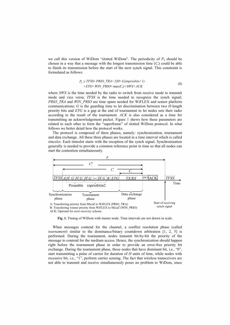
we call this version of WiDom “slotted WiDom”. The periodicity of PS should be chosen in a way that a message with the longest transmission time (Ci) could be able to finish its transmission before the start of the next synch signal. This constraint is formulated as follows:

sP TFSS+PRIO_TRA+2(H+G)(npriobits+1) +ETG+WIN_PRIO+max(Ci)+SWX+ACK

(1)

where SWX is the time needed by the radio to switch from receive mode to transmit mode and vice versa; TFSS is the time needed to recognize the synch signal; PRIO_TRA and WIN_PRIO are time spans needed for WiFLEX and sensor platform communications; G is the guarding time to let discrimination between two H-length priority bits and ETG is a gap at the end of tournament to let nodes sets their radio according to the result of the tournament. ACK is also considered as a time for transmitting an acknowledgement packet. Figure 1 shows how these parameters are related to each other to form the “superframe” of slotted WiDom protocol. In what follows we better detail how the protocol works.

The protocol is composed of three phases, namely: synchronization, tournament and data exchange. All these three phases are located in a time interval which is called timeslot. Each timeslot starts with the reception of the synch signal. Synchronization generally is needed to provide a common reference point in time so that all nodes can start the contention simultaneously.

Fig. 1. Timing of WiDom with master node. Time intervals are not drawn in scale.

When messages contend for the channel, a conflict resolution phase (called tournament) similar to the dominance/binary countdown arbitration [1, 2, 5] is performed. During the tournament, nodes transmit bit-by-bit the priority of the message to contend for the medium access. Hence, the synchronization should happen right before the tournament phase in order to provide an error-free priority bit exchange. During the tournament phase, those nodes that have dominant bit, i.e., “0”, start transmitting a pulse of carrier for duration of H units of time, while nodes with recessive bit, i.e., “1”, perform carrier sensing. The fact that wireless transceivers are not able to transmit and receive simultaneously poses no problem to WiDom, since

Tournament phase

A: Transferring priority from MicaZ to WiFLEX (PRIO_TRA) B: Transferring winner priority from WiFLEX to MicaZ (WIN_PRIO) ACK: Optional for error recovery scheme

TFSS A H G H G ... G H H G B ETG TX/RX TFSS Time

Start of receiving synch signal

Synchronization phase

(npriobit)x2

Data exchange phase

Preamble

sP

iC

iC iC

SWX ACK

when a node has a dominant bit, there is no need for reception and when a node has a recessive bit, it just performs carrier sense. There is also a guarding time interval G to separate pulses of carrier’s wave. This guarding time interval makes the protocol robust against clock inaccuracies and takes into account that signals need some (non-zero) time to propagate from one node to another. If a node loses the contention of a bit (i.e., it has a recessive bit and receives a dominant bit), it does not continue sending further bits and only proceed listening to the medium to find out the priority of the winner. If a node does not lose the contention during the current bit it will proceed with the contention for the next bit. At the end of the tournament, the node that does not receive a pulse wins the competition and waits for ETG time units before starting data transmission.

There are three important issues that deal with the add-on circuitry which is used in the new implementation of WiDom: (i) In the tournament phase, before going through the competition, the priority of the enqueued message should be notified to the WiFLEX board and at the end of the competition, the priority of the winner should be reported back to the WSN host platform. Thus, in the slotted WiDom, we need to consider two time intervals (A and B) for internal communications between the two boards. (ii) Only those nodes that have messages in their queues wait for receiving the synch signal; this means that if a node enqueues a message slightly after the synch signal broadcast, it will not participate in the current on-going tournament, even if the tournament phase formally has not started, yet. (iii) Due to hardware shortcomings [6], it is needed to introduce some bit stuffing after each priority bit and according to the same reason two dominant bits instead of a single one should be sent as preamble, to indicate the start of the contention period.

In the following section, we will present the response time analysis for slotted WiDom according to the described timings.

3 Calculating Response Time

The schedulability analysis presented in this paper borrows ideas from the previously published CAN analysis [7]. It provides feasibility tests, based on Worst Case Response Time (WCRT) computation. However, our analysis is non-trivial and slightly different from [7], since we deal with (i) error detection, using acknowledgment (Ack) packets rather than (six) consecutive identical symbols, and (ii) the slotted nature of the protocol. The WCRT of a message stream is the longest response time of all message instances q that enter the ready queue for a period of time called level-i busy period. A level-i busy period is a time interval [t0, t1) such that both t0 and t1 are beginning of a timeslot and considering only non-faulty timeslots (i.e., timeslots where all the three phases perform normally without any error occurrence) in [t0, t1) it holds that for each timeslot, either (i) all transmitted packets have higher priority than mi, or (ii) at most one transmitted packet with lower priority than mi is transmitted in the first timeslot (started at t0). Figure 2 shows an example of a level-i busy period. Our preliminary WiDom analysis presented in [2] is simplistic in that:

It is assumed that no transmission error can happen. It is not realistic to ignore the transmission errors especially for error-prone wireless channel, when providing pre-run-time guarantees for safety-critical applications.

It does not consider the release jitter that generally occurs while messages are being queued.

Fig. 2. Level-i busy period; lower index shows higher priority. The upward arrow indicates the release time of the message.

Consequently, following the analysis in [7], we observe that the WCRT of an instance q of a message stream mi can be divided into four components: 1. wi,q, which corresponds to the longest time interval from the start of the busy

period till when the instance q starts a successful transmission — see Figure 3. 2. iC , as the time span needed to finish a transmission, which includes the

tournament duration and time needed to detect the synch signal — see Figure 1. 3. Ji, as release jitter or queuing jitter [8], which is defined as the largest difference

between the initiating time of an event and the time at which the message, triggered by the event, has been queued.

4. EOi, as error overheads, including the time for receiving Ack packets, the re-transmission time and the duration of noise burst which is provoked by an interference source.

Fig. 3. An example of wi,q.

To compute the response time of message stream mi in slotted WiDom, we consider a busy period of [t0, t1) interval. According to the definition, there should be a packet transmission in all non-faulty timeslots during the [t0, t1) interval. We observe that, according to the release time of messages in high or low priority sets, it is possible to have different cases which result in various response time equations. All

0,2q

Tx

Tx 1,1q

Time

Stream m2

1,2q

Tx 1,2 2Qq

...

1,2w

Stream m1 Tx 0,1q

Tx

Level-i Busy Period

Stream m1

Stream m2

Stream mi

Stream mi+1 Tx

Tx

Tx

Tx

Time t0 t1

Ps Ps Ps Ps

these cases are shown in Table 1. In order to reduce the level of pessimism in our calculation, we investigate each case individually and then derive the appropriate response time equations for each of them. Finally the maximum of the response times over all these cases gives a tight bound on the WCRT for a set of message streams.

Table 1. Different cases of WCRT computation. lp(i) / hp(i) corresponds to the set of message streams with priority lower / higher than the message stream mi.

Message in lp(i) arrived in [t0-PS, t0)?

Message mi arrived in [t0-PS, t0)?

Message in hp(i) arrived in [t0-PS, t0)?

Case 1 No No No Case 2 No No Yes Case 3 No Yes No Case 4 No Yes Yes Case 5 Yes No No Case 6 Yes No Yes Case 7 Yes Yes No Case 8 Yes Yes Yes

Case 1. Considering there is no message released in [t0-PS, t0) interval which is the last timeslot immediately before, the level-i busy period begins. This is the simplest case where there is neither blocking from the lp(i) set nor further interfering from the hp(i) set. We can compute the WCRT for the message stream mi as follows:

iiiCase

Qq

Casei TqCJwR

qiCasei

1

1,...,0

1,1

max (2)

where iC is the time span needed to finish transmission can be obtained by the following:

iC =TFSS+PRIO_TRA+2(H+G)(npriobits+1)+ETG+WIN_PRIO+ Ci (3)

and wi,q represents the longest time from the start of busy period until when the instance q of the message stream mi begins a successful transmission. It is obvious that the erroneous transmission can lead to a longer delay. Therefore, it should include the error recovery overhead and can be formulated as follows:

iCase

qiisihpj j

bitjCase

qis

Caseqi CwEP

TQJw

Pqw 1,

)(

1,1

, (4)

Ei( t) is the maximum time required for error signaling and recovery scheme in any time interval of length t. The error model, Ei( t), will be described in the following section. The number of instances Qi, of message stream mi that become ready for transmission before the end of busy period is given by:

11

1

i

iCaseiCase

i TJLQ (5)

where Li is the length of the longest level-i busy period and can be computed by:

1

)(

11 Case

iisiihpj j

jCaseiCase

i LEPT

JLL . (6)

To investigate the remaining cases, we follow same equations as shown above and rewrite only those equations that are different. Note that in each case we should replace the appropriate superscript in the response time equations.

Case 2. Consider that there is an instance of hp(i) message released in [t0-PS, t0) interval. This case is rather similar to Case 1 except that we need to consider more interference imposed by the hp(i) message. Therefore, Ri and Qi can be calculated similar to Case 1 but we must consider the following changes in wi,q and Li computation:

iCase

qiisihpj j

bitjsCase

qis

Caseqi CwEP

TQJPw

Pqw 2,

)(

2,2

,

(7)

2

)(

22 Case

iisiihpj j

jsCaseiCase

i LEPT

JPLL . (8)

Case 3. In this case we have neither hp(i) nor lp(i) message instances in [t0-PS, t0) interval, but the instance of message mi is released in [t0-PS, t0) slightly after synch signal broadcast. As described in Section 2, only nodes with non-empty ready queue wait to receive synch signal, thus, message mi misses participating in the current tournament phase and should wait for the next timeslot. This case is almost similar to Case 1 but we need to add the duration of one timeslot to Equation 2. So we will have:

siiiCase

Qq

Casei PTqCJwR

qiCasei

3

1,...,0

3,3

max . (9)

Case 4. Assume that there is no lp(i) message released in [t0-PS, t0) interval, but both hp(i) and mi messages are released during this interval. With the same reasoning as Case 2 we revise the Equation 4 and 6 by considering the following equation for Ri calculation:

siiiCase

Qq

Casei PTqCJwR

qiCasei

4

1,...,0

4,4

max (10)

iCase

qiisihpj j

bitjsCase

qis

Caseqi CwEP

TQJPw

Pqw 4,

)(

4,4

,

(11)

4

)(

44 Case

iisiihpj j

jsCaseiCase

i LEPT

JPLL . (12)

Case 5. Consider that there is only one instance of lp(i) released in [t0-PS, t0) interval and there is neither any instance of message mi nor any hp(i) message in this time interval. We can follow the same equation as we had in Case 1 and then introduce the blocking term in the computation of wi,q and Li. Thus we have:

iCase

qiisihpj j

bitjCase

qiss

Caseqi CwEP

TQJw

PqPw 5,

)(

5,5

, (13)

5

)(

55 Case

iisiihpj j

jCasei

sCasei LEP

TJL

PL . (14)

Case 6. In this case both hp(i) and lp(i) messages are released in [t0-PS, t0) interval. Knowing that the low priority message is suppressed by the higher priority one, we can consider this case exactly similar to Case 2 where there is no lp(i) message instance released.

Case 7. Assume that there is no hp(i) message in [t0-PS, t0) interval, but both lp(i) and message mi are released during this interval. It is clear that the lp(i) cannot impose any blocking to the response time calculation, thus this case is equivalent to Case 3.

Case 8. Consider that an instances of hp(i), lp(i) and the message stream mi are released in [t0-PS, t0) interval. Following the same rationale as in last two cases, lp(i) is suppressed by higher priority messages which results in similar equations as Case 4.

Therefore, by studying all the possible scenarios and observing that the response time in Case 4 is no less than the response times of cases 1, 2 and 3, the WCRT of message stream mi can be calculated as follows:

54 ,max Casei

Caseii RRR . (15)

4 Error model

Besides physical aspects related to signal propagation, in the wireless channel a communication error may result from the interference due to various transmitters sharing the same frequency band, like Wi-Fi, Bluetooth and other sensor networks. It may also come from the presence in the close area of electromagnetic sources such as, e.g., electric motors and microwave ovens. To minimize the impact of external interferers on the reliability of the system, we implement an error recovery scheme based on Ack packets sent after each data packet. Thus, if the sender does not receive back from the receiver an Ack packet during a predefined period of time, it will re-issue the data transmission, i.e., by retrying from the next tournament and retransmit the data until it receives the Ack from the intended receiver1. It should be mentioned that the retransmission of the corrupted packet may not happen immediately after the erroneous transmission, since a higher priority message may be enqueued while waiting for the Ack of the previous transmission.

A fully asynchronous noise burst can cause a transmission error: an error happens when a node is transmitting either a data packet or an Ack packet. As it is shown in Figure 4, a noise burst with length of one timeslot PS can impose a penalty of up to 2PS on the response time.

Fig. 4. Error caused by a noise burst with length of one timeslot.

Given P(L) as a function that computes the penalty of an occurring L-length error, a burst of noise with duration of Le can give rise to the following penalty on the response time:

1 Note that, the error recovery method that we used for WiDom is not exactly like what is done

in CAN bus. We do not need to globalize a detected error since in this version of WiDom we are dealing with the unicast transmission not multicast. To save more resources we also do not assign an individual timeslot for sending the Ack packet since the Ack packet size is comparatively smaller than data packet size and can be transmitted during the current timeslot.

TFSS TRNM ACK TX/RX Time

TFSS TRNM ACK TX/RX

PS PS

Noise Burst

Noise Burst

sss

ee PP

PLLP )( . (16)

Assuming that F( t) is an error function that models the interference in wireless channel during time interval t, then, the maximum additional delay caused by the error recovery scheme can be given by:

Ei( t)= P(Le)F( t) . (17)

Unfortunately, no widely-accepted error model has been proposed for a real-time data traffic over wireless channels so far – an important research issue that is beyond the scope of this paper. As a consequence, similarly to the technique proposed in [9], we consider two different types of noise sources: (i) periodic noise burst with the period of Terror and the burst length of Lerror, and (ii) sporadic noise burst with minimum inter-arrival time of Ts_error and burst duration of Ls_error. The sporadic noise, models the interference caused by packet-based radios (e.g., Wi-Fi, Bluetooth) and the periodic noise represents the interference induced by other electromagnetic devices. So, by considering K sources of periodic noise bursts and J sources of sporadic noise bursts, the overall delay during the time interval t due to the error recovery process is given by [9]:

Table 2 summarizes all the symbols used in the analytical section and their corresponding definitions.

5 Experimental Evaluations

In this section, we evaluate the existing WiDom protocol against the implementation of a novel and more reliable version: the Ack-enabled WiDom. To the best of our

J

i

ierrorsi

errors

K

i

ierrori

errori LP

TtLP

TttE

1_

_1)()()( . (18)

Table 2. Symbols used in the equations Ri WCRT for message stream i Li The length of level-i busy period

Qi Number of instances in message stream i that become ready for transmission

during Li period Wi,q Time span from start of busy period until instance q start transmission

Ji Release jitter of message stream i Ci”

Time needed to finish the transmission of a message in message stream i Ti The periodicity of message stream i PS The periodicity of synchronization signal

P(Le) The penalty of an Le-length error occurring

Ei( t) Extra time overhead imposed by the error recovery mechanism during a time interval t

knowledge, this is the first reported implementation of WiDom (either slotted or unslotted) with an acknowledgement mechanism. In the following subsections we first detail the implementation of Ack-enabled WiDom, then we discuss the experimental setup and finally show the results from a real test bed and compare them against the theoretical analysis reported in the previous sections.

5.1 Implementation and practical aspects

We implemented the Ack-enabled WiDom in the Nano-RK operating system [14]. Nano-RK is a Real-Time Operating System (RTOS) designed for wireless sensor networks. It employs an energy-efficient time management scheme using one-shot timer interrupts, instead of polling interrupts. Due to this policy, the scheduler executes with the periodicity of such timer, i.e., approximately every 1 ms. Consequently, every time-related events, such as task periods and event wake-ups, will experience at most a 1 ms jitter with respect to their targeted time. Nevertheless, to enhance the accuracy of our estimations, such a jitter factor has been taken into account into our analytical computations.

Each sender node has three periodic tasks running on Nano-RK: Send-Task, Receive-Task and Management-Task, whose pseudo-codes are presented in Algorithm 1 to 3, respectively. By each request of Send-Task a variable called Gnt_N is incremented by one. This variable records the number of requests for packet transmission generated during an experiment. The arrival time of each request is stored in the variable Gnt_T, in order to check the possibility of retransmissions, in case of an unsuccessful data exchange. Since the tournament phase is performed by a WiFLEX board, i.e., an ad-hoc add-on hardware [4], which is shared by the above

Algorithm 1. Send-Task Algorithm 2. Receive-Task

1: while true do 2: 3: Gnt_N++ 4: 5: SendPkt() 6: SSent 7: false 8: Wait until next period 9: end while 10: 11: Procedure SendPkt() 12: if successful access to hardware=1 then 13: if my_ID= winner_ID then 14: if this is an original transmission then 15: Txed_N++ 16: end if 17: transmit the packet over radio 18: 19: end if 20: end if

1: while true do 2: if TTSRCV= false then 3: Wait until next period 4: else 5: Wait to receive the Ack packet 6: if received Ack is correct then 7: SSent 8: end if 9: 10: 11: Wait until next period 12: end if 13:end while

tasks, the access to that resource needs arbitration. This has been implemented by regulating the way the tasks call a SendPkt() function, through a global flag (LockSend), which is set by the Send-Task only. Through the SendPkt() function the nodes start contending for the channel. Based on the WiDom protocol, each node uses its given ID number as its packet priority and if two or more nodes access the channel at the same time, the collision is resolved by the given priorities. As a result, if a node wins the tournament it sends its packet and then “activates” the Receive-Task in order to wait for the reception of the corresponding acknowledgment packet. To do so, it sets a global flag (TTSRCV, time to start receiving) to TRUE — see Algorithm 1, line 18.When the Receive-Task is executed, two conditions might hold: (i) the global flag TTSRCV has not been set, then the task suddenly exits, or (ii) the flag has been set by the Send-Task. In the latter case, the node switches to receive mode and waits to receive an Ack packet. If the received Ack packet is the expected one, i.e., it contains the correct information including source ID and sequence number of the recent data transmission, then the global flag “SSentFlag” (i.e., successful sent) is set to TRUE. Either the Ack has been received or not, the Receive-Task ends up by “activating” the Management-Task to execute — see Algorithm 2, line 10. Similarly, the Management-Task encounters one of two situations when it requests to be executed. The first situation occurs when the “TTSMNG” flag (time to start managing) is FALSE; in this case the task is released to the scheduler and waits for the next activation — see Algorithm 3. The second situation occurs when the “TTSMNG” is TRUE and it usually happens after a transmission of data packet and a miss in the reception of an Ack packet. Then, if the TTSMNG is TRUE, a retransmission is needed and the first step is to get the current time and check if there is enough time for performing a retransmission. To do so, it is needed to compute the elapsed time by subtracting the current time from the Gnt_T time recorded at the beginning of the Send-Task. If there is enough time to have another slot with duration of PS before the next activation of Send-Task (which is defined by the Send-Task period), then it is possible to retransmit the packet. However, the retransmission

Algorithm 3. Management-Task Table 3. Tasks’ configuration

1:while true do 2: if TTSMNG = false then 3: Wait until next period 4: else 5: 6: - Gnt_T 7: if Elapsed_T > (SND_task.period - Ps) then 8: if SSentFlag = 0 then 9: if LockSend = false then 10: SendPkt() 11: end if 12: end if 13: end if 14: 15: Wait until next period 16: end if 17:end while

Send_Task_prio 2 Send_Task_period MSG-Period Send_Task.SchType NONPREEMPTIVE Receive_Task_prio 3 Receive _Task_period 15 ms Receive _Task.SchType PREEMPTIVE Managemant_Task_prio 4 Managemant_Task_period 15 ms Managemant _Task.SchType PREEMPTIVE

should be performed if the SSentFlag is still FALSE. In this case, the task calls the SendPkt() function ensuring that the shared resource is currently available. Taking advantage of locks and flags we are able to target an efficient way to control the execution of each task at right moments. Table 3 shows the values Nano-RK allows to set for each task’s configuration. Note that: (i) a small number in Task_prio implies higher priority, and (ii) the period of the Send_Task defines the data rate of the nodes in each experiment.

When a packet has no chance to be transmitted within its deadline, it is said that a deadline miss event occurred. In order to estimate how often this happens, at the end of each experiment the difference between the number of generated packets (i.e., Gnt_N) and the number of actually transmitted packets (i.e., Txed_N) is computed. Similarly, to measure the response time, each node measures the delay between the instant of the Send-Task execution until the actual packet transmission. Then this delay (Wi) piggybacks within the packet payload. Since we have used a hardware-timer with time resolution of 1 µs, all the measured values have the accuracy of 1 µs. Upon receiving a packet, the receiver extracts the Wi and computes the response time (Ri) according to the following expression:

Ri=Wi+Ci , (19)

where Ci is the duration of the data exchange phase (refer to Figure 1). With the help of sniffer devices [10] and a custom–designed log file’s parser, built

in C and bash programming, we are able to measure the packet loss ratio and the WCRT-miss ratio. Furthermore, to enrich the comparison of the performance between the classical WiDom and the novel Ack-based protocol, the energy consumed by the nodes at different data rates is also shown. Finally, to better appreciate the trade-offs between the performance indices, the behavior of the packet loss ratio against the energy consumption is presented.

5.2 Experimental Setup

We have conducted several experiments by varying the interference level in the environment. Our testbed consists of 10 MicaZ motes [11] (featuring an Atmel ATmega128L 8-bit microcontroller with 128 kB of in-system programmable memory and 4 kB of available RAM memory) equipped with the WiFLEX add-on board [4]. An extra MicaZ mote acts as a gateway: this node is always waiting to receive data from the other nodes and never participates in the tournament phase to send back the acknowledgement packets, so it doesn’t need to be equipped with any extra hardware — see Figure 5.

Each one of the 10 MicaZ equipped with the WiFLEX board is configured to run at a different data rate (i.e., MSG-Period as in Table 3) or a different priority. For instance, Node1’s MSG-Period is T1=70 ms, Node2’s MSG-Period is T2=180 ms and so on, while for the last three nodes2 it holds T8=T9=T10=5.4 s (refer to Tables 5-8).

The data packets’ length is set to 128 bytes (including PHY, MAC headers, CRC and payload) since it is the maximum packet length supported by the CC2420 radio [12] on board of MicaZ platform. The length of Ack packets is 17 bytes. Given these

2 For the last three nodes only the priority (given by the node’s ID) is different.

figures and considering the maximum data rate over the wireless medium of 250 Kb/s at the ISM band of 2.4 GHz [12], the time needed to transmit a data packet is:

sCni i 4096250000

18128:...1

(20)

In the same way, the time needed to transmit an Ack packet is 554 . Applying Equation (3) we have:

sCni i 9158:...1 (21)

This value is computed with the timeouts given in Table 4, experimentally measured from the real platform. Considering (i) npriobits=15 and all the mentioned timeout values and (ii) the constraint in Equation (1), the periodicity of the synch signal, PS, should be larger than 9747 s. We choose the PS =15 ms, i.e., the master node sends a 300 s-long synch signal every 15 ms. We relaxed this choice to allocate to the gateway some time to accomplish the data extraction from the received packet and to format the customized Ack packet. Consequently, the nodes were configured with different transmission rates ranging from 190 bps to 14 kbps. Interestingly, these choices give analytical system utilization values ranging between 39% and 92.2%.

5.3 Observations

We utilize different interference patterns to evaluate the reliability and robustness of WiDom protocol against noise, while having a predictable response time for message streams. Our evaluation focuses on five network performance indices as follows: Packet loss rate: the ratio of the received data packets over all the sent packets. Deadline miss ratio: the ratio of messages that missed their deadlines over the total number of generated messages. In all scenarios, the deadline is considered to be implicit which is equal to the message periodicity. WCRT miss ratio: the ratio of messages that have been sent after their calculated WCRT over the total number of generated messages.

Table 4. Timeout values.

Parameter Value

GH s110 TFSS s300

TRAPRIO _ s238 PRIOWIN _ s449

ETG s555

SWX s35

Fig. 5. Experimental setup

Average response time: the average of all received messages response time on the gateway from any sender. Energy consumption: the average energy consumption for each node, expressed as a function of the number of packets sent and received.

We run the experiment for both classical and Ack-enabled version of WiDom in different noisy environments. All experiments were run for around 40 minutes, which corresponds to more than 40,000 message transmission requests.

5.3.1 Interference pattern We create two types of interference to test WiDom protocol: (i) periodic interference and (ii) sporadic interference. The periodic interference is usually spatially localized and follows a regular duty cycle pattern. The best example is the interference produced by microwave ovens. To create this noise pattern we utilize the Jamlab tool [13] running on an extra MicaZ node. We set the interferer’s duty cycle to 70 ms and 200 ms to compare the performance of WiDom protocol under different noise densities. We refer to the environment with higher noise burst rate as High Noisy Channel (HNC) scenario — see Figure 6(a), and the one with with lower noise burst rate as Low Noisy Channel (LNC) scenario — see Figure 6(b). Both periodic interferers send three packets with length of 128 bytes in burst to occupy the channel for the duration of one slot, PS = 15 ms — considering data rate of 250 Kb/s. The sporadic noise model emulates in a fully controlled way the interference coming from heavily loaded WiFi access points. To generate this interference traffic, we used a simple model inspired by the Markov model presented in [9], consisting of two states: “clear channel” and “interference”. However, in our model, instead of having a complete randomness and irregularity of the interference signal, we imposed a fixed duration of staying in the “interference” state, in order to have the same burst length — equal to one time slot PS. To define the time duration for staying in the “clear channel” state we have used a constant value of 5 ms multiplied by a random variable R which is uniformly distributed over [14, 200]. Hence, the time duration of staying on the clear channel state will be a random time period from 70 ms to 1 s. In other words the minimum inter-arrival time between two consecutive noise bursts is set to 70 ms. We refer to this scenario as Sporadic Noisy Channel, SPNC — see Figure 6(c). All interferers generate noise in the channel 15 of the IEEE 802.15.4 spectrum. In all scenarios, interferers are generating packets and transmitting them with the highest power level (0 dBm). As it is shown in the spectrum analyzer (Figure 6), the radiation power in all situations are the same, but the density of noise bursts are quite high in the Figure 6(a) compared to that on Figure 6(b). It can be also observed that in the presence of a sporadic noise source, the channel spends more time in clear channel state compared to the periodic noise source with duty cycle of 70 ms. Note that the spectrum analyzer visualizes the status of the entire Zigbee bandwidth, including the noise coming from WiFi/IEEE 802.11 wireless routers on the adjacent channels.

5.3.2 Results and discussion Packet loss rate. Figure 7 depicts the packet loss rate for both version of protocols in different noise conditions. Here two observations can be made. First, the packet loss rate for Ack-enabled WiDom is much smaller than that of classical version of WiDom

Fig. 6. Spectrum occupancy in presence of a periodic interferer with duty cycle of 70 ms (a) and 200 ms (b) and in presence of a sporadic interferer with minimum inter-arrival time of

70 ms (c). The spectrum analyzer also shows the effect of IEEE 802.11 wireless routers on the adjacent channels.

(a)

(b)

(c)

Zigbee Channels

Am

plitu

de [d

Bm

]

Am

plitu

de [d

Bm

]

Zigbee Channels

Am

plitu

de [d

Bm

]

Zigbee Channels

protocol in every scenarios. This is thanks to the implementation of Ack packets which provide a legitimate feedback on transmission status for the sender nodes, giving them a chance for retransmitting the lost packets. It is also shown that the high noisy channel jeopardizes the network performance much more than the low noisy channel or the SPNC case. As it is illustrated on Figure 7, SPNC is less destructive, since the packet loss rate in SPNC is about 2% lower than that in the HNC. Two reasons contribute to this: (i) in high noisy channel there is a higher risk of collision for both data and Ack packet; (ii) higher collision rate consequently leads to more retransmission requests that increases the traffic load. The second observation is that in each scenario the packet loss rate is almost flat against the data rate. There might be an expectation that for higher transmission rate there ought to be higher loss rate. It is true that higher data rates experience a greater number of packets lost, but Figure 7 clearly shows that in terms of packet loss rate (percentage) the performance is almost independent from the data rate. Moreover, the implementation of Ack-enabled mechanism helps in achieving fairer performance for all data rates than the classical WiDom. Timing behavior. There are three distinct metrics that are investigated under the time domain. Table 5, Table 6 and Table 7 show the results achieved from the experimental setup of WiDom in HNC, LNC and SPNC interference environments. The first metric is the deadline miss ratio and shows the number of generated packets which did not have the chance to be transmitted. It has been observed that for all scenarios there is no deadline miss for any message stream — the two variables Gnt_N and Txed_N were always equal!

The WCRT miss ratio is the second timing metric considered. It indicates the number of messages which have been sent with response time higher than their analytically computed WCRT. The analytically calculated response time is shown by Calc. Ri on the tables. It has been computed by applying the response time analysis to calculate the upper-bound of response time for each message stream according to Equation (2)-(15).

Fig. 7. Packet loss ratio of Ack-enabled WiDom and classical WiDom.

Table 6. Response time in LNC.

i 1 2 3 4 5 Protocol

implementation Ack-enabled

WiDom Classical WiDom

Ack-enabled WiDom

Classical WiDom

Ack-enabled WiDom

Classical WiDom

Ack-enabled WiDom

Classical WiDom

Ack-enabled WiDom

Classical WiDom

Ti( s) 70,000 180,000 350,000 700,000 1,200,000 Data rate(bit/s) 14,629 5,689 2,926 1,463 853

Calc.Ri( s) 55,158 25,158 70,158 40,158 100,158 55,158 115,158 70,158 130,158 100,158 Exp. Avg. Ri( s) 17,769 13,932 20,020 16,061 19,342 18,994 26,118 20,187 33,916 22,956 Exp. Max. Ri( s) 53,122 23,159 59,232 33,809 80,596 44,296 94,604 55,271 108,183 73,483

i 6 7 8 9 10 Ti( s) 1,900,000 3,700,000 5,400,000 5,400,000 5,400,000

Data rate(bit/s) 539 277 190 190 190 Calc.Ri( s) 145,158 115,158 175,158 130,158 205,158 145,158 265,158 175,158 280,158 205,158

Exp. Avg. Ri( s) 35,303 29,103 38,711 29,801 37,509 37,001 40,080 40,127 45,397 40,741 Exp. Max. Ri( s) 118,599 94,601 142,268 104,367 163,848 96,682 168,064 105,221 184,175 82,168

Table 5. Response time in HNC.




Ack-enabled WiDom

Classical WiDom

Ack-enabled WiDom

Classical WiDom

Ack-enabled WiDom

Classical WiDom

Ack-enabled WiDom

Classical WiDom



i 6 7 8 9 10 Ti( s) 1,900,000 3,700,000 5,400,000 5,400,000 5,400,000



Table 7. Response time in SPNC.




Ack-enabled WiDom

Classical WiDom

Ack-enabled WiDom

Classical WiDom

Ack-enabled WiDom

Classical WiDom

Ack-enabled WiDom

Classical WiDom



i 6 7 8 9 10 Ti( s) 1,900,000 3,700,000 5,400,000 5,400,000 5,400,000


Exp. Avg. Ri( s) 35,604 29.014 38,868 29,462 42,191 39,218 46,713 40,793 47,508 41,921 Exp. Max. Ri( s) 132,047 93,261 153,510 102,286 185,420 82,490 181,506 83,912 181,241 85,122

Table 8. Response time for classical WiDom in non-lossy environment.

i 1 2 3 4 5 Ps ( s) 10,000 15,000 10,000 15,000 10,000 15,000 10,000 15,000 10,000 15,000

Ti( s) 30,000 70,000 70,000 180,000 120,000 350,000 300,000 700,000 900,000 1,200,000 Data rate(bit/s) 34,133 14,629 14,629 5,689 8,533 2,926 3,413 1,463 1,138 853


i 6 7 8 9 10 Ti( s) 1,900,000 1,900,000 3,700,000 3,700,000 5,400,000 5,400,000 5,400,000 5,400,000 5,400,000 5,400,000

Data rate(bit/s) 539 539 277 277 190 190 190 190 190 190 Calc.Ri( s) 110,158 115,158 120,158 130,158 170,158 145,158 180,158 175,158 200,158 205,158


We have used the timeouts given in Subsection 5.2 and a value for the jitter3 of 1 s. The maximum and average value of response time obtained through the

experiment for each message stream are shown by Exp. Max. Ri and Exp. Avg. Ri , respectively. From a comparison between the values of Calc. Ri and Exp. Max. Ri , it is confirmed that no message has shown a response time higher than the calculated WCRT in all the considered scenarios, which substantiates the fact that the analytical model for the WCRT provides a fairly good upper bound to the expected response time. Moreover, looking at Exp. Avg. Ri in Table 5, 6 and 7, i.e., the average value of response time, it is evident how the Ack-enabled mechanism slightly increases the response time for all the message streams. As expected, this is what the system pays to achieve the good results shown in Figure 7 in terms of packet loss ratio. Moreover, while the classical WiDom is almost indifferent to the various noise patterns, from the tables it can be observed that, a higher noise density leads to higher response time for the Ack-enabled WiDom. These results are totally expected, because as the noise density increases, there are more packet collisions and consequently higher number of retransmissions. As anticipated, the average values of the response time of message streams are similar for the classical WiDom, in any channel condition. The reason is that there is no mechanism devised in classical WiDom which takes into account the noise of the channel. Nodes sends their packet only once according to their arrival schedules and there is no feedback to let them know about their transmission status.

The last observation leads us to run another experiment for classical WiDom in non-lossy environment in order to push the system to its limits. Since we are using the classical WiDom there is no need to consider extra time for the gateway to process received data packet and to issue an Ack packet. Hence, the synchronization period can be safely decreased from PS=15 ms to, e.g., PS=10 ms, i.e., a value closer to the theoretical limit computed in Section 5.2. Accordingly, the data rate of the first five message streams can be increased.

Table 8 shows the timing behavior of protocol in such a non-lossy environment, with a noise floor of -96 dBm. Once more, no packet loss has been observed nor deadline miss and no WCRT miss ratio were reported. Observing the values of Table 8 it is also evident that by shrinking the synchronization period, we could slightly achieve better timing behavior, while accommodating nodes with higher data rates. This leads to the conclusion that in a non-lossy environment (interference probability reduced to 0) or for non-loss sensitive applications, it is preferable to use the classical WiDom approach, since it can provide better timing behavior.

Finally, Figure 8 summarizes the previous findings by showing the average response time as a function of the data rate in all interference scenarios. As confirmed by the above analysis of the tables, the average response time in Ack-enabled WiDom is higher than that of classical WiDom protocol in all scenarios. It appears clear that the higher noisy channel deteriorates the average response time compared to lower noisy channel for the Ack-enabled WiDom protocol, while the average response time for the classical WiDom protocol does not change significantly under different noise

3 We remind that Nano-RK [14] uses a policy of scheduling the tasks and interrupts with a one-

shot timer whose accuracy is 1 µs. Then all tasks might experience a jitter of around 1 µs delay for any execution.

conditions. Finally, when the environment is non-lossy, it is possible to get smaller average response time values by implementing the classical WiDom protocol also through the reduction of the synchronization period, PS, which allows for higher data rates.

Energy cost. As we have discussed earlier, implementing Ack mechanism

increases the reliablity of WiDom protocol and makes it robust in noisy environment, despite an increase in the response time. Nevertheless, we should also consider the cost of extra energy consumption due to the exchange of extra packets. In particular, there are two major sources of energy cunsumption in Ack-enabled WiDom compared to the classical WiDom case: (i) the amount of energy for receiving the Ack packet and (ii) the extra cost for retransmitting after an unsuccessful transmission. Cosidering the current draw of 19.7 mA in receive mode and 14 mA in transmit mode (transmission power level 19) of MicaZ mote [11], the normalized energy consumption for Ack-enabled WiDom is estimated as follows:

E(Ack-enabled WiDom) = )14

7.19(17)_(128)__( AckPktNoTxPktNoRTxPktNo

(22)

Fig. 8. Average response time for Ack-enabled and classical WiDom in HNC, LNC and SPNC environments and classical WiDom in non-lossy environment with PS =15 ms and PS = 10 ms and different data rates.

where No_RTxPkt represents the number of retransmitted 128 bytes-long packets, No_AckPkt indicates the number of 17 bytes-long Ack packets received by the nodes and No_TxPkt is the number of transmitted packets. Similarly, the normalized energy consumption of classical WiDom can be estimated as follows:

E(Classical WiDom) = 128)_( TxPktNo (23) so, the extra energy we pay for implementing the Ack-enabled WiDom against the classical WiDom for same number of transmission request is:

Energy loss ratio [%] = E(Ack-enabled WiDom) - E(Classical WiDom) 100 E(Classical WiDom)

. (24)

We do not consider the extra cost paid by the gateway node to receive retransmissions and send back Ack packets. This makes sense under the common assumption that the gateway is provided with an extra energy supply. As it is shown in Figure 9, the extra energy cost of using the Ack-enabled mechanism is roughly between 25% and 35%, compared with the classical WiDom, for any data rate. It can be seen that the energy loss shows some fluctuations at lower data rates and tends to stabilize as the data rate increases. The reason is that nodes at lower data rate may have the opportunity to experience disruptive bursts of interference more often than the others, then they may need to retransmit more to deliver their messages successfully.

In terms of the impact of the interference pattern, it is evident that the higher noise density conditions imposes higher energy consumptions due to the higher number of retransmissions. The energy loss rate is about 10% higher for HNC scenario compared to that in LNC environment, while the SPNC case shows performance similar to the LNC interference pattern.

Finally, to better understand the impact of the ack-based mechanism, we have compared the packet loss rate against the power consumption (assuming as a simplification that the time to transmit a byte is equal to the time to receive one) — see Figure 10. The average power consumption has been computed knowing the duration of each experiment. Note that the number of transmission request is different in each scenario. That is why we have different power consumption for classical WiDom. However, the number of transmission requests for both Ack-enabled and classical WiDom protocol is the same under the same channel condition. The

Fig. 9. Energy loss ratio for Ack-enabled WiDom vs. classical WiDom in HNC, LNC and SPNC environments.

comparison of the two implementations under the same channel condition proves once more that by spending around 30% of more energy it is possible to keep the data loss ratio below 2%, even in the worst interference conditions.

6 Concluding remarks

In this paper, we focused on a prioritized MAC protocol, WiDom, recently proposed for Wireless (Sensor) Networks and opted for a more recent low overhead implementation of this MAC design that is called slotted WiDom. Our primary contribution was to develop a sufficient response time analysis for slotted WiDom with message streams that suffer from release jitter and also experience noise in the channel. We have shown that our analysis is non-trivial due to the slotted nature of the protocol and in order to reduce the level of pessimism in the calculated upper bound, we should individually explore all the possible cases that may happen according to the arrival pattern of message streams and then pick the maximum upper bound among all possible cases. Another contribution of this paper was to offer error recovery scheme to make the protocol more robust and reliable in noisy environment. We considered an Ack-based implementation of the protocol and developed the analysis according to this modification. To validate our calculated upper bounds we have conducted a set of experiments in different channel conditions. The experimental results have shown that implementing Ack-enabled WiDom reduces the packet loss rate remarkably, to less than 2%, under high noisy channel compared to the classical WiDom protocol. The results further certified our findings in the analytical calculations that the theoretical analysis offers a valid upper-bound for each message streams. According to the analysis, having Ack-enabled WiDom increases the average response time that is verified through the experiments. It has also shown that having Ack-enabled WiDom intensifies energy consumptions (as number of data transmissions and retransmissions). In fact, there is a trade-off between having lower response time, lower energy consumptions and reliable data transmissions: this leads to an optimization problem at design time,

Fig. 10. jfjyk.

Fig. 10. Packet loss ratio vs. average power consumption for Ack-enabled WiDom and classical WiDom in HNC, LNC and SPNC environments.

where the system designer can choose the most appropriate solution according to the application needs or (expected) channel conditions.

References

1. Bosch. CAN Specification version 2.0. Robert Bosch GmbH, Pstfach 30 02 40, D-70442 Stuttgart (1991)

2. Pereira, N., Andersson, B., Tovar, E.: WiDom: a Dominance Protocol for Wireless Medium Access. J. TII. 3, 120--130 (2007)

3. Andersson, B., Tovar, E.: Static-Priority Scheduling of Sporadic Messages on a Wireless Channel. In: 9th International Conference on Principles of Distributed Systems, pp. 322--333. IEEE Press, Italy (2005)

4. Pereira, N., Gomes, R., Andersson, B., Tovar, E.: Efficient Aggregate Computations in Large-Scale Dense WSN. In: 15th IEEE Real-Time and Embedded Technology and Applications Symposium, pp. 317--326. IEEE Press, San Francisco (2009)

5. Mok, A., Ward, S.: Distributed Broadcast Channel Access. J. Com. Net. 3, 327--335 (1979)

6. Gomes, R.: Efficient Implementation of a Dominance Protocol for Wireless Medium Access. Technical report, MSc Thesis, Polytechnic Institute of Porto, (2008)

7. Davis, R., Burns, A., Bril, R., Lukkien, J.: Controller Area Network (CAN) Schedulability Analysis: Refuted, Revisited and Revised. J. RTS. 35, 239--272 (2007)

8. Tindell, K., Hansson, H., Wellings, J.: Analysing real-time communications: controller area network (CAN). In: 15th IEEE Real-Time Systems Symposium, pp. 259--263. IEEE Press, Puerto Rico (1994)

9. Boano, C.A. , Voigt T., Tsiftes N., Mottola L., Römer K., Zuniga M.: Making Sensornet MAC Protocols Robust Against Interference. In: 7th European Conference on Wireless Sensor Networks, pp. 272--288, Portugal (2010)

10. Z-monitor: A monitoring tool for ieee 802.15.4 wireless personal area networks, 2010. (http://www.z-monitor.org).

11. CROSSBOW-Datasheet: MICAz. San Jose, USA. Crossbow Technology, Inc., 2004. 12. T. Instruments, “CC2420 datasheet,” http://focus.ti.com/lit/ds/symlink/cc2420.pdf. 13. Boano, C.A., Voigt, T., Noda, C., Romer, K., and Zuniga, M.: Jamlab: Augmenting

sensornet testbeds with realistic and controlled interference generation. In IPSN 2011.

http://www.z-monitor.org/

http://focus.ti.com/lit/ds/symlink/cc2420.pdf

technical report - cister - research centre in real-time

Documents