technical report crwr 264 an evaluation of the …
TRANSCRIPT

Technical Report
CRWR 264
AN EVALUATION OF THE FACTORS AFFECTING THE QUALITYOF HIGHWAY RUNOFF IN THE AUSTIN, TEXAS AREA
by
LYNTON B. IRISH, JR., P.E.
WILLIAM G. LESSO, Ph.D.
and
MICHAEL E. BARRETT, M.S.,Project Manager
JOSEPH F. MALINA, JR., P.E.Principal Investigator
and
RANDALL J. CHARBENEAU, P.E.GEORGE H. WARD, Ph.D.Co-Principal Investigators
September 1995
CENTER FOR RESEARCH IN WATER RESOURCES
Bureau of Engineering Research •• The University of Texas at AustinJ.J. Pickle Research Campus •• Austin, TX 78712

ii

iii
ACKNOWLEDGMENTS
This research was funded by the Texas Department of Transportation (TxDOT)
and the Civil Engineering Department at the University of Texas at Austin through grant
number 7-1943, “Water Quantity and Quality Impacts Assessment of Highway Runoff
and Construction in the Austin, Texas Area.”

iv

v
TABLE OF CONTENTS
ACKNOWLEDGMENTS...................................................................................... iii
TABLE OF CONTENTS ....................................................................................... v
LIST OF TABLES ................................................................................................. ix
LIST OF FIGURES ............................................................................................... xi
1.0 CONCLUSIONS AND RECOMMENDATIONS ........................................ 1
2.0 INTRODUCTION ......................................................................................... 7
2.1 Research Area......................................................................................... 7
2.2 Research Objective ................................................................................. 7
2.3 Highway Runoff Constituents ................................................................. 8
2.4 Highway Runoff Constituent Build-Up Mechanisms............................... 13
2.5 Constituent Removal Mechanisms .......................................................... 18
2.6 Highway Constituent Discharge Theory.................................................. 20
2.7 Summary ................................................................................................ 27
3.0 DATA COLLECTION .................................................................................. 29
3.1 Introduction ............................................................................................ 29
3.2 Rainfall Simulation ................................................................................. 29
3.3 Rainfall Simulator Design....................................................................... 32
3.4 Rainfall Simulator Operation .................................................................. 42
3.5 Water Quality Sampling.......................................................................... 45
3.6 Runoff Constituents ................................................................................ 50
3.7 Flow Measurement ................................................................................. 51
3.8 Event Mean Concentration...................................................................... 53
3.9 Rainfall Measurement............................................................................. 54
3.10 Miscellaneous Measurements.................................................................. 55
3.11 Detection Limit Data .............................................................................. 55
3.12 Summary .............................................................................................. 56
4.0 DATA SUMMARY ....................................................................................... 59
4.1 Introduction ............................................................................................ 59
4.2 Storm Event Characteristics .................................................................... 59

vi
4.3 Distribution of Highway Runoff EMCs................................................... 69
4.4 Descriptive Statistics............................................................................... 74
4.5 Constituent Wash-Off Patterns................................................................ 80
4.6 First Flush............................................................................................... 84
4.7 Daily and Seasonal Variations................................................................. 84
4.8 Street Sweeping Variations ..................................................................... 84
4.9 Summary ................................................................................................ 90
5.0 MODEL DEVELOPMENT .......................................................................... 93
5.1 Introduction ............................................................................................ 93
5.2 Selection of an Appropriate Modeling Technique.................................... 96
5.3 Identification of Relevant Model Variables ............................................. 99
5.4 Worksheet Development......................................................................... 103
5.5 Covariance, Correlation and Causation ................................................... 105
5.6 Model Misspecification........................................................................... 106
5.7 Variables Included in the Model ............................................................. 107
5.8 Summary ................................................................................................ 109
6.0 MODEL RESULTS....................................................................................... 111
6.1 Introduction ............................................................................................ 111
6.2 Results of the Regression Analysis.......................................................... 111
6.3 Model Verification with Data from the Convict Hill Site......................... 123
6.4 Interpretation of the Regression Results .................................................. 1246.4.1 Solids .......................................................................................... 1296.4.2 Oxygen Demand / Organics......................................................... 1316.4.3 Nutrients ..................................................................................... 1316.4.4 Metals ......................................................................................... 132
6.5 Summary ................................................................................................ 133
GLOSSARY ........................................................................................................... 135
BIBLIOGRAPHY .................................................................................................. 137
APPENDICES ........................................................................................................ 143
APPENDIX A: Laboratory Analysis .................................................................... 145
APPENDIX B: Precipitation Characteristics for Austin, Texas ............................ 147

vii
APPENDIX C: Water Droplet Trajectory............................................................. 149
APPENDIX D: Probability Plots.......................................................................... 153
APPENDIX E: Histograms of Constituent Event Mean Concentrations ............... 167
APPENDIX F: Constituent Wash-Off Patterns .................................................... 175
APPENDIX G: The Method of Generalized Least Squares: Corrections forHeteroscedasticity and Autocorrelation ....................................... 189
APPENDIX H: Residual Histograms.................................................................... 211
APPENDIX I: Regression Results ...................................................................... 219

viii

ix
LIST OF TABLES
Table Page
1.1 Variables Affecting Pollutant Runoff Loads ................................................. 3
2.3.1 Reported Median Constituent Concentrations in Urban Runoff ..................... 13
2.3.2 Metals in Highway Runoff............................................................................ 14
3.1.1 Highway Characteristics at the MoPac Test Sites.......................................... 30
3.4.1 Flow Rate (L/s) Given Nozzle Diameter (mm) and Pressure (kpa) ................ 44
3.4.2 Rainfall Intensities Produced by Selected Spray Head NozzleSizes and Pressures....................................................................................... 45
3.4.3 Rainfall Simulator Actual Operating Parameters........................................... 47
3.5.1 Median Background Constituents ................................................................. 50
3.6.1 Highway Runoff Constituents....................................................................... 51
4.2.1 Characteristics of Simulated Storm Events (Traffic Sessions) ....................... 60
4.2.2 Characteristics of Simulated Storm Events (No-Traffic Sessions) ................. 61
4.2.3 Characteristics of Sampled Natural Storm Events (West 35th St. Site).......... 65
4.2.4 Characteristics of Sampled Natural Storm Events (Convict Hill)................... 67
4.4.1 Event Mean Concentrations for Simulated Rainfall Events with Traffic........ 75
4.4.2 Event Mean Concentrations for Simulated Events without Traffic ................ 76
4.4.3 Event Mean Concentrations for Natural Rainfall Events at theWest 35th Street Sampling Site..................................................................... 77
4.4.4 Event Mean Concentrations for Natural Rainfall Events at theConvict Hill Sampling Site ........................................................................... 78
4.4.5 Median Event Mean Concentrations (mg/L) ................................................. 79
4.6.1 First Flush of Highway Runoff Constituents ................................................. 87
4.8.1 Computed Street Sweeping t-Statistics.......................................................... 90
5.3.1 Relevant Model Variables............................................................................. 103
5.5.1 Correlation Coefficients Between Suspected Causal Variables andConstituent Load (g/m2) ............................................................................... 106
6.2.1 Summary of Model Coefficients (Non-Metals) ............................................. 112
6.2.2 Summary of Model Coefficients (Metals) ..................................................... 113
6.2.3 Street Sweeping Shifts .................................................................................. 117

x
6.2.4 Expected Loads Based on MoPac Street Sweeping Program ......................... 118

xi
LIST OF FIGURES
Figure Page
2.6.1a Observed COD Build-Up......................................................................... 21
2.6.1b Observed COD Wash-Off ........................................................................ 21
2.6.2 Theoretical Wash-Off Pattern .................................................................. 27
3.3.1 Relationship Between Nozzle Pressure, Splash Plate Design,Attack Angle, and Droplet Size................................................................ 36
3.3.2 Spray Head Assembly.............................................................................. 39
3.3.3 Spray Stand Assembly ............................................................................. 40
3.3.4 Total Rainfall Simulator Assembly .......................................................... 43
3.4.1 The Rainfall Simulator at MoPac and West 35th Street, Austin, Texas(a) View of the Rainfall Simulator in Operation; (b) The StormwaterSampling Station ..................................................................................... 46
3.5.1 Simulated Storm Sampling Scheme ......................................................... 48
3.7.1 Rating Curve for Highway Curb at MoPac and West 35 Street ................ 53
4.2.1 Distribution of Uncontrolled Variables during Rainfall Simulation(a) Storm Event Runoff (L/m2); (b) Number of Vehicles duringthe Storm Event ....................................................................................... 63
4.2.2 Distribution of Controlled Variables during Rainfall Simulations(a) Duration of the Antecedent Dry Period (hrs); (b) Traffic Countduring the Antecedent Dry Period............................................................ 64
4.2.3 Distribution of Natural Rainfall Event Variables (a) Event Rainfall (mm);(b) Distribution of Natural Rainfall Event Variables ............................... 66
4.2.4 Rainfall / Runoff Relationship (a) West 35th Street Sampling Site;(b) Convict Hill Sampling Site................................................................ 68
4.3.1 Normal and Lognormal Probability Plots for the TSS Data(a) TSS Normal Probability Plot; (b) TSS Log Probability Plot.............. 71
4.3.2 Histogram of TSS Observations............................................................... 72
4.3.3 Histogram of Nitrate Observations........................................................... 72
4.3.4 Histogram of Oil and Grease Observations .............................................. 73
4.5.1a Median TSS Concentration During a Simulated Storm Event................... 81
4.5.1b Median TSS Load During a Simulated Storm Event ................................ 81
4.5.1c TSS Load During Natural and Simulated Storm Events ........................... 81
4.5.2a Median Nitrate Concentration During a Simulated Storm Event .............. 82

xii
4.5.2b Median Nitrate Load During a Simulated Storm Event ............................ 82
4.5.2c Nitrate Load During Natural and Simulated Storm Events ....................... 82
4.5.3a Median Oil and Grease Concentration During a Simulated Storm Event .. 83
4.5.3b Median Oil and Grease Load During a Simulated Storm Event ................ 83
4.5.3c Oil & Grease Load During Natural and Simulated Storm Events ............. 83
4.6.1a Load vs. Flow for Solids and Nutrients .................................................... 85
4.6.1b Load vs. Flow for Organics and Oil and Grease ....................................... 85
4.6.1c Load vs. Flow for Metals ......................................................................... 85
4.6.2a Percent Load vs. Flow for Solids and Nutrients........................................ 86
4.6.2b Percent Load vs. Flow for Organics and Oil and Grease........................... 86
4.6.2c Percent Load vs. Flow for Metals............................................................. 86
4.7.1a Seasonal Variation (July, 1993 - July, 1994), TSS ................................... 88
4.7.1b Seasonal Variation (July, 1993 - July, 1994), Nitrate ............................... 88
4.7.2a Hourly Variation (July, 1993 - July, 1994), TSS ...................................... 89
4.7.2b Hourly Variation (July, 1993 - July, 1994), Nitrate .................................. 89
5.2.1 Exponential Function Fit to the Data Collected at theWest 35th St. Sampling Site..................................................................... 97
5.2.2 Observed TSS Load vs. Predicted TSS Load using Duration of theAntecedent Dry Period and the Intensity of the Preceding Stormas Causal Variables.................................................................................. 98
6.2.1 TSS Model Results (a) Fit of Data from West 35th Street Site;(b) Model Residuals vs. Total Rainfall .................................................... 119
6.2.2 COD Model Results (a) Fit of Data from West 35th Street Site;(b) Model Residuals vs. Total Rainfall .................................................... 120
6.2.3 Nitrate Model Results (a) Fit of Data from West 35th Street Site;(b) Model Residuals vs. Total Rainfall .................................................... 121
6.2.4 Zinc Model Results (a) Fit of Data from West 35th Street Site;(b) Model Residuals vs. Total Rainfall .................................................... 122
6.3.1 TSS Model Predictions (a) Model Prediction at the Convict Hill Site;(b) Prediction Error vs. Total Rainfall ..................................................... 125

xiii
6.3.2 COD Model Predictions (a) Model Prediction at the Convict Hill Site;(b) Prediction Error vs. Total Rainfall ..................................................... 126
6.3.3 Nitrate Model Predictions (a) Model Prediction at the Convict Hill Site;(b) Prediction Error vs. Total Rainfall ..................................................... 127
6.3.4 Zinc Model Predictions (a) Model Prediction at the Convict Hill Site;(b) Prediction Error vs. Total Rainfall ..................................................... 128

1
1.0 Conclusions and Recommendations
The Center for Research in Water Resources at The University of Texas at Austin
has conducted a four-year investigation of the quality of storm water runoff from existing
highway pavements in and near the recharge zone of the Barton Springs segment of the
Edwards Aquifer. The two goals of this research project were to identify the variables
that affect the build-up and wash-off of constituents from highways in the Austin, Texas
area and to develop a water quality model that incorporates these variables. The research
was funded by the Texas Department of Transportation and the Department of Civil
Engineering at The University of Texas at Austin through grant number 7-1943, “Water
Quantity and Quality Impacts Assessment of Highway Construction in the Austin, Texas
Area.”
Isolation of the variables that influence highway runoff quality is facilitated
during “steady-state” storm conditions (e.g., a constant rate of constituent input from
rainfall and traffic). A unique rainfall simulator was used to produce steady-state storm
events during this research. The rainfall simulator provided a uniform rainfall over a
230-meter length of 3-lane highway during periods of active traffic. The entirety of the
runoff drained to a single curb inlet where water quality samples were collected
throughout the simulation. The length of highway exposed to the artificial rainfall
allowed for collection of water that had washed from the bottoms of the moving vehicles.
This project marked the first scientific use of a rainfall simulator in conjunction with
active traffic.
Thirty-five rainfall simulations were conducted between July 6, 1993 and July 14,
1994. Additionally, 23 natural storm events were sampled at the same location between
September 14, 1993 and April 28, 1994. Statistical analysis showed no significant
difference between the runoff generated by the rainfall simulator and the natural runoff.
The samples collected during simulated and natural storm events combined to provide
423 storm water runoff observations. Furthermore, 21 variables were identified for each
storm event, and multiple regression analysis was used to determine the relationship of
each variable to the quality of the highway runoff. The variables found to be statistically
significant were retained for use in a constituent-specific regression model.

2
The majority of variations observed in highway storm water loading in the Austin
area may be explained by causal variables measured during the rain storm event, the
antecedent dry period, and the previous rain storm event. Significant causal variables
during the rainfall event include the duration of the event (min), the volume of runoff per
area of watershed (L/m2), the intensity of the runoff per area of watershed (L/m2/min),
and the average volume of traffic per lane. The significant causal variables from the
antecedent dry period include the duration of the dry period (hrs) and the average volume
of traffic per lane during the dry period. The significant causal variables from the
preceding storm event include the duration of the event (min), the volume of runoff per
area of watershed (L/m2) and the intensity of the runoff per area of watershed (L/m2/min).
The identification of the causal variables that significantly influence constituent
loading is among the more important findings of this study. There are two major
applications of this knowledge. First, recognition of the specific variables that influence
a given constituent load may suggest constituent-specific mitigation procedures, and
second, the applicability of the model is directly reflected in the causal variables.
Because the dependent variable in the regression analysis is expressed as load
(g/m2), the total volume of flow during the storm event will appear in every constituent
model. Similarly, the intensity of the runoff and the duration of the runoff also will
frequently appear in the models. The variables flow, intensity, and storm duration,
therefore, offer little diagnostic information in the interpretation of the model
specification. However, the appearance of the other variables in the model, such as the
number of vehicles during the storm, the duration of the antecedent dry period, and the
volume of runoff during the previous storm event, are variables that “control” the
constituent loading. The examination of the controlling variables in each model adds
insight into the applicability of the model and the mitigation of constituent loading. A
summary of selected water quality constituents and their relevant causal variables is
presented in Table 1.1.

3
Table 1.1 Variables Affecting Pollutant Runoff Loads
StormDuration
StormVolume
StormIntensity
VehiclesDuringStorm
Length ofAntecedent Dry Period
AntecedentTrafficCount
PreviousStorm
Duration
PreviousStorm
Volume
PreviousStorm
Intensity
Iron * * *
TSS * * * *
Zinc * * * * * *
COD * * * * *
Phosphorus * * * *
Nitrate * * *
BOD5 * * * *
Lead * * * *
Copper * * *
Oil andGrease
* *
As an example, 93% of the variation observed in the storm water loadings of total
suspended solids (TSS) is explained by the total volume of storm water runoff (L/m2),
intensity of the runoff (L/m2/min), total duration of the antecedent dry period (hrs), and
the intensity of the runoff during the previous storm event (L/m2/min). This model
formulation suggests that the conditions during the antecedent dry period (e.g., dustfall,
pavement/right-of-way maintenance activities, etc.) and the intensity of the preceding
storm event (e.g., the thoroughness of the previous wash-off) have a greater influence on
TSS storm water loadings than any of the other variables examined, including the traffic
volume during the storm event. Efforts to mitigate the storm water loading of TSS
should therefore be directed at activities during the antecedent dry period that deposit dirt
and debris on the highway surface. Consequently, street sweeping was found to be
effective at reducing TSS loads. Street sweeping on a once every two-week schedule, as
compared to no street sweeping, significantly reduced the average loads of TSS observed
in the highway storm water runoff. However, no other constituent showed a significant
change in loading during the street sweeping period.
Highway runoff constituents, in general, fall into one of three categories: (1) those
constituents, such as TSS, which are influenced by conditions during the dry period and
may be mitigated by dry period activities such as street sweeping and others; (2) those

4
constituents that are most influenced by conditions during the rainfall event and may only
be mitigated through the use of runoff controls; and (3) those constituents that are
influenced equally by both periods. The constituents that are significantly affected by
conditions during the preceding storm event generally are those constituents that are
controlled by the dry period variables.
The variables found to significantly affect the other highway runoff constituents
are detailed below:
• Nutrients: The total duration of the storm event (min), total volume of storm waterrunoff (L/m2), intensity of the runoff (L/m2/min), and the total volume of trafficduring the antecedent dry period (a measure of the length of the dry period) combineto explain 95% of the variation in nitrate load, and 90% of the variation in totalphosphorus load, observed in the highway runoff. This regression formulation isstrongly influenced by the quantity of these nutrients contained in the rainfall. Theconcentrations of nutrients observed in rainfall accounted for 50% to 100% of thenitrate load, and up to 22% of the total phosphorus load observed in the highwayrunoff. The mitigation of nutrients in highway runoff requires the use of runoffcontrols.
• Organics: The total duration of the storm event (min), total volume of storm waterrunoff (L/m2), runoff intensity (L/m2/min), total volume of traffic during the storm,and the total volume of traffic during the antecedent dry period combine to explain86% of the biochemical oxygen demand (BOD5) load, 95% of the chemical oxygendemand (COD) load, 94% of the total carbon load, and 91% of the dissolved totalcarbon load observed in the highway runoff. The mitigation of organics must beaccomplished with runoff controls.
• Oil and Grease: The total volume of storm water runoff (L/m2) and the total volumeof traffic during the storm combine to explain 94% of the variation in the oil andgrease loads observed in the highway runoff. The mitigation of oil and grease mustbe accomplished with runoff controls.
• Copper: The total duration of the storm event (min), total volume of storm waterrunoff (L/m2), and total volume of vehicles during the storm combine to explain 90%of the variation in the copper load observed in the highway runoff. The mitigation ofcopper must be accomplished with runoff controls.
• Lead: The total volume of storm water runoff (L/m2), runoff intensity (L/m2/min),total volume of vehicles during the storm, and the intensity of the previous stormrunoff (L/m2/min) combine to explain 68% of the variation in the lead load observedin the highway runoff. The mitigation of lead must be accomplished with runoffcontrols.

5
• Iron: The total volume of storm water runoff (L/m2), runoff intensity (L/m2/min) andthe total duration of the antecedent dry period (hrs) combine to explain 92% of thevariation in the iron load observed in the highway runoff. The mitigation of iron mustbe accomplished with dry period practices.
• Zinc: The total duration of the storm event (min), total volume of storm water runoff(L/m2), volume of vehicles during the antecedent dry period, total duration of theprevious storm (min), and the total volume of storm water runoff in the previousstorm (L/m2) combine to explain 92% of the variation in the zinc load observed in thehighway runoff. The mitigation of zinc must be accomplished with both runoffcontrols and dry period practices.
Although traffic volume during the storm does not appear as a “significant”
variable in every model formulation, it is nevertheless an influential factor in all
constituent loading. The storm water constituent wash-off patterns for high speed
highway pavements were found to be different during periods when traffic is on the
highway than during periods when there is no traffic. The runoff from pavements with
high speed traffic does not exhibit as pronounced a “first flush” of constituent mass as the
runoff of pavements without traffic. The continuous input of material from traffic insures
a continual increase in the cumulative constituent load throughout the duration of the
storm event. As a result, highway watersheds that contain large shoulder areas or other
non-traffic bearing surfaces (e.g., > 35% of the total watershed) can be expected to
produce less constituent loading per unit of surface area than other highway pavements.

6

7
2.0 Introduction
2.1 Research Area
The State of Texas, through the Texas Natural Resource Conservation
Commission (TNRCC), regulates all activities that have the potential to cause pollution
in the Edwards Aquifer (Chapter 313 entitled “Edwards Aquifer,” Subchapter B,
§313.27). This rule applies to any activity that alters or disturbs surface water quality and
quantity characteristics within the recharge zone of the aquifer. The construction of
highways, railroads, utility services, and residential/commercial developments are all
regulated activities under Chapter 313. Consequently, the Texas Department of
Transportation (TxDOT) is charged with the responsibility for the control of storm water
runoff from highway construction sites and from existing highways located inside the
Edwards Aquifer recharge zone. Exercising this responsibility has had a profound impact
on the design and construction of area highways. During fiscal year 1993, the Austin
District of TxDOT spent more than $10 million on the installation and construction of
temporary and permanent runoff control facilities. The cost of storm water control now
accounts for as much as 20% of the overall cost of highway construction in the Edwards
Aquifer recharge zone. This financial burden has placed a new importance on
understanding the role of the urban highway as a non-point source of water pollution in
the Austin area.
2.2 Research Objective
Controlling the cost of storm water management along highways in the Edwards
Aquifer recharge zone is a major concern of TxDOT. Cost-effective and efficient
management practices to mitigate the transport of harmful constituents to the aquifer are
dictated by fiscal and environmental concerns. The environmental concerns in the
Edwards Aquifer, in conjunction with the high cost of complying with a pollution
prevention policy whose goals are not easily understood, have motivated TxDOT to
undertake an extensive investigation of the water quality aspects of storm water runoff
from highways in or near the Barton Springs segment of the Edwards Aquifer recharge
zone. Identification of the variables that determine constituent loads in highway runoff is

8
the first step in determining the most cost-effective mitigation methods. Development of
predictive models will further assist cost-effective analyses of highway storm water
management practices in the Edwards Aquifer recharge zone.
The objectives of this research are:
• the determination of the variables that affect the build-up and wash-off ofconstituents from highways in the Austin, TX area,
• the development of a predictive model that incorporates the variables thataffect runoff quality.
The methodology of model development is the subject of this report. The
underlying theory of the build-up and wash-off of materials from highway surfaces is
presented in this chapter. The rationale for data collection and the manner in which data
were collected is discussed in Chapter 3. A summary of the data is presented in Chapter
4. The formulation of the model is detailed in Chapter 5; the results of the model
presented are given in Chapter 6. Appendices provide supporting data and
documentation.
2.3 Highway Runoff Constituents
The bulk of the material on urban roadways consists of inert minerals such as
quartz, feldspar, etc. (Sartor and Boyd, 1972). The quantities of these particles correlate
well with the average daily traffic count (Hvitved-Jacobson and Yousef, 1991), although
atmospheric dustfall also may be a major source (Gupta et al., 1981). Stormwater runoff
that carries solids from highway surfaces is undesirable for several reasons:
1. High sediment loads increase the probability of transportingnutrients, pesticides, organic constituents, and microbial forms thatmay be attached to the particles (Svensson, 1987; Wagner andMitchell, 1987; Sartor and Boyd, 1972).
2. The deposition of solids can clog recharge features and restrict theflow of water into the aquifer (Guadalupe-Blanco River Authority,1988)
3. The Edwards Aquifer contains a number of invertebrates and at leastone vertebrate. The build-up of silt in submerged caverns mayinterfere with organism metabolism (Guadalupe-Blanco RiverAuthority, 1988).

9
Several classifications of solids have been observed for highway runoff. The total
solids (TS) content of a sample is defined as the amount of material remaining after
evaporation of the water or a steam bath followed by drying the sample to a constant
weight at 103o - 105oC. Total suspended solids (TSS) is the fraction of total solids that
is retained on a filter with a pore size of about 1.2 micrometers (µm). Volatile suspended
solids (VSS) consists of the organic fraction of TSS. Highway runoff studies typically
report values for both TSS and VSS.
Organic material is the next most common constituent in highway runoff.
Biodegradable organics may stimulate the growth of bacteria in receiving watercourses.
In the worse case, the oxygen consumed during the biochemical oxidation of organic
matter can deplete the dissolved oxygen in the receiving stream to the point of causing
septic conditions and destroying populations of fish and other aquatic species that require
dissolved oxygen.
The organic content of runoff may be expressed as BOD, COD, and total organic
carbon (TOC). The BOD analysis is a bioassay procedure that provides suitable living
conditions for bacteria to function in an unhindered fashion (i.e., all necessary nutrients
for bacteria growth must be present and there must be an absence of toxic substances).
The test is a direct measure of the oxygen consumed by bacteria during the oxidation of
organic matter in a measured time period. Five days is the typical test period, and the
results are denoted as BOD5. Durations of up to 20 days, however, are also employed.
The COD analysis measures the ability of organic material to be reduced by a
strong oxidizing agent (potassium dichromate) at an elevated temperature. Organic
matter is oxidized during the test regardless of the biological assimilability of the
substances. COD values are therefore greater than BOD5 values for most compounds.
The COD may be much greater when the organic matter is resistant to biological
degradation.
The TOC is the total amount of organic carbon in the runoff. Carbon in runoff is
oxidized to carbon dioxide with a catalyst and oxygen as the carrier gas; carbon dioxide
is then measured using an infrared analyzer. The TOC analysis is rapid and is applicable
to low concentrations of organic matter.

10
The dissolved oxygen content in natural surface waters also is affected by the
input of nutrients to the water body. Nitrogen and phosphorus are the primary nutrients
observed in highway runoff that can stimulate algal blooms in receiving waters. The
sources of nutrients typically include atmospheric deposition and the application of
roadside fertilizers (Hvitved-Jacobson and Yousef, 1991). The concentration of nitrogen
and phosphorus in highway runoff is a concern for two reasons; (1) these compounds
stimulate the growth of aquatic plants in surface waters and (2) excessive nitrates (NO3)
in drinking water can cause methemoglobinemia in infants.
The enrichment of a surface water with nutrients, or eutrophication, is a natural
aging process that results in the increased growth of planktonic and rooted aquatic plants.
During the daylight hours, aquatic plants convert inorganic nutrients and CO2 into
organic plant material through the process of photosynthesis. The process will continue
as long as nutrients are available to maintain plant growth. The dissolved oxygen (DO)
produced during photosynthesis is generally beneficial to the surface water ecosystem,
but an over-abundance of plant growth can result in severe DO problems. Excess
vegetation, in the most extreme cases, can produce exaggerated diurnal variations in
dissolved oxygen that results in supersaturated levels of DO during daylight hours and
extremely low levels of DO as the plants respire at night. An additional oxygen demand
is exerted as the plant matter dies and decays. Excessive aquatic plant growth also may
be aesthetically objectionable and can interfere with the biological, recreational, and
navigational use of the water.
Phosphorus is not known to be harmful outside of stimulating plant growth. The
control of phosphorus, however, may be important in areas where natural surface waters
contain low concentrations of phosphorus relative to the nitrogen concentration. Both
phosphorus and nitrogen are required to sustain maximum growth of aquatic plants and
the nutrient that is in short supply therefore limits the growth aquatic plants. If
phosphorus is the “limiting” nutrient in the receiving stream, additional discharges of
phosphorus may promote new plant growth.
Nitrogen compounds can cause problems other than aquatic plant growth. Un-
ionized ammonia is toxic to several species of young freshwater fish (USEPA, 1981), but
the greater concern is the contamination of drinking water sources with nitrates.

11
Excessive nitrates in drinking water can cause methemoglobinemia in very young infants.
Nitrates have a negative charge (NO3) and, therefore, are not attracted to soils, which also
have negative charges. It is for this reason that nitrogen in the form of nitrate usually
reaches the ground water, where it is very mobile due to its solubility and anionic form.
Metals are the most common toxicants found in highway runoff. The sources of
metals in highway runoff include vehicles, atmospheric deposition, naturally occurring
metals in soils, and highway-related sources such as paint and corrosion products (Gupta
et al., 1981; Yousef et al., 1886). The two major concerns with trace metals are: (1) these
elements may move through soils and enter ground water and (2) metals can accumulate
in the food chain. It should be noted that metals are not necessarily toxic; however,
unless the concentration causes toxicity (e.g., metals at low concentrations are essential to
the human diet).
The most common metals found in highway runoff are copper, iron, lead, and zinc
(Sartor and Boyd, 1972; Gupta et al., 1981; USEPA, 1983; Driscoll et al., 1990).
Chromium, which is found in small concentrations, is most likely in the reduced form of
the chromate ion (Cr3+), which is much less toxic than the highly oxidized form (Cr6+)
found in plating shop wastes (Driscoll et al., 1990). Arsenic, cadmium, mercury, and
nickel are found in relatively insignificant amounts (Sartor and Boyd, 1972; Gupta et al.,
1981). Iron is not known to be harmful; however, the iron concentrations normally
observed in highway runoff are higher than those reported in natural water systems
(Driscoll et al., 1990).
Pathogenic organisms that potentially are responsible for waterborne diseases
such as typhoid and paratyphoid fever, dysentery, diarrhea, and cholera, have been
observed in highway runoff (Sartor and Boyd, 1972; Gupta et. al., 1981). The Barton
Springs segment of the Edwards Aquifer is potentially sensitive to the presence of
pathogenic organisms. The aquifer is used as a drinking water source, and Barton Creek
is used by the public for swimming and boating.
It is difficult to identify specific pathogenic organisms in a water sample. The
number of pathogens in a normal sample usually is very small and it is difficult to isolate
the pathogens from the other bacteria in the sample. Water quality samples are analyzed
for “indicator organisms” that signify the potential presence of pathogens. Total coliform

12
(TC), fecal coliform (FC), and fecal streptococci (FS) are indicators used in
bacteriological analyses of water. Fecal coliforms and fecal streptococci are bacteria
found in the digestive tract of warm-blooded animals. The presence of fecal coliforms
and fecal streptococci may be an indication of pathogenic organisms. Additionally, the
ratio of fecal coliforms to fecal streptococci may be used to determine the origin of the
contamination. Domestic animals have a FC/FS ratio that is less than 1.0, whereas the
ratio for humans is typically greater than 4.0 (Metcalf & Eddy, Inc., 1991). A total
coliform count includes both the fecal coliforms and the coliforms found in soils.
Coliforms generally die off quite rapidly in receiving waters (Sartor and Boyd,
1972). Bacteria also are removed from runoff streams by filtration, adsorption,
desiccation, radiation (sunlight), predation by other bacteria, and exposure to other
adverse conditions (USEPA, 1981). Therefore, any relationship between the number of
coliforms on the highway surface and the number that may be found in adjacent receiving
streams is difficult at best.
Other parameters and constituents of concern in highway runoff include pH,
temperature, total dissolved solids, oil and grease, and pesticides and herbicides. Values
of pH reported by Driscoll et al. (1990) ranged from 5.5 to 7.5, with an average of 6.5.
Discharges within this pH range are not known to cause water quality problems.
Temperature is of concern only if runoff volumes are large enough to severely alter the
temperature of the receiving stream. Total dissolved solids (TDS) may be a concern if
the highway runoff results in an increase in the salinity of the receiving water. TDS
could be a concern during snow melt in areas where highways are heavily salted to aid in
ice removal.
Oil and grease concentrations reported by Driscoll et al. (1990) ranged from 5
mg/L to 10 mg/L. There is no evidence that oil and grease at these concentrations are
harmful to human health and the environment.
Pesticides (chlorinated hydrocarbons) were found in significant quantities in street
runoff by Sartor and Boyd (1972). However, this class of constituents was not addressed
in this study.
The median constituent concentrations observed in highway runoff are
summarized in Tables 2.3.1 and 2.3.2.

13
2.4 Highway Runoff Constituent Build-Up Mechanisms
Highway runoff characterization studies have been conducted in the United States
for over 30 years. A massive amount of data relating to the quality of runoff from urban
pavements has been generated. An evaluation of the available literature suggests that the
sources of constituents in highway runoff can be categorized as: (1) vehicular
contributions, (2) atmospheric deposition, and (3) the road bed material. The relationship
of each source to the quality of the storm water runoff is very complex and not well
understood.
Table 2.3.1 Reported Median Constituent Concentrations in Urban Runoff
Constituent Median Concentration
pH 5.5 - 7.5 (a)
TSS 142 mg/L (0.62) (a)
VSS 39 mg/L (0.58) (a)
BOD5 5 mg/L - 25 mg/L (a)
COD 114 mg/L (0.58) (a)
Total Carbon 25 mg/L (0.62) (a)
Kjeldahl Nitrogen 1.83 mg/L (0.45) (a)
NO2 + NO3- 0.76 mg/L (0.56) (a)
PO4 - P 0.40 mg/L (0.89) (a)
Total Coliform 260/100ml - 180,000/100ml (b)
Fecal Coliform 20/100ml - 1,900/100ml (b)
Fecal Streptococci 940/100ml - 27,000/100ml (b)
Oil & Grease 5 mg/L - 10 mg/L (a)
Number in parenthesis is the reported coefficient of variation(a) - Driscoll et al. (1990); (b) - Gupta et al. (1981)

14
Table 2.3.2 Metals in Highway Runoff
Metal Concentration inHighway Runoff
(µγ/Λ)
%Dissolved
Drinking WaterStandard (µγ/Λ)
Cadmium 1 - 30 (c)
72% (e) 10 (a)
Chromium 15 - 35 (c)65%
(e)(Cr6+) 50 (a)
Copper 54 (0.68) (c)70%
(e) 1,000 (b)
Iron 3,000 - 12,000 (c)27%
(e) 300 (b)
Lead 400 (1.46) (c)21%
(e) 50 (a)
Mercury 0.001 - 1.5 (c) Not Reported 2 (a)
Nickel 150 (d)76%
(e) Not Established
Zinc 329(0.44) (c)57%
(e) 5,000 (b)
Number in parenthesis is the reported coefficient of variation(a) USEPA Primary Drinking Water Standards(b) USEPA Secondary Drinking Water Standards(c) Driscoll et al. (1990). A single value represents the site median EMC for all urban highway sites.(d) Gupta et al. (1981)(e) Yousef et al. (1986)
The source of the constituents in highway runoff is influenced by environmental
conditions that are often difficult, if not impossible, to measure. Some of the constituents
can be traced to more than one source, in which case it is often difficult to distinguish the
dominant source. The build-up process of constituents in highway runoff is further
complicated by a continuous and complex removal process. During dry weather,
materials are continually blown on and off the highway, as well as on and off of vehicles
by natural and vehicle induced winds. During wet weather, storm water washes
constituents from both the highway surface and the vehicles. Although physical transport
is thought to be the primary method of constituent removal, there is certainly some
chemical or biological removal that occurs on the highway surface (i.e., volatilization,
chemical decay, biodegradation, etc.).
Highway constituent loads are thought to be closely related to the average daily
traffic (ADT) count of the highway. Sartor and Boyd (1972) identified the following list
of vehicle contributions:
1) Leakage of fuel, lubricants, hydraulic fluids, and coolants;
2) Fine particles worn off of tires and clutch and brake linings;
3) Particulate exhaust emissions;

15
4) Dirt, rust, and decomposing coatings that drop off of fender liningsand undercarriages;
5) Vehicle components broken by vibration or impact (glass, plastic,metals, etc.).
ADT is a measure of highway usage. The high ADT highways, such as urban
expressways, typically produce higher constituent concentrations than the low ADT
highways that are normally located in rural areas. Driscoll et al. (1990) found a
statistically significant difference in the constituent concentrations at sites with an ADT
greater than 30,000 and those with an ADT less than 30,000. However, it is difficult to
segregate the influence of traffic from that of the surrounding land use since lighter traffic
sites tend to be more rural than heavier traffic sites. A lack of a clear correlation with
ADT within each group led Driscoll et al. (1990) to the conclusion that surrounding land
use is a more important influence than traffic. Stotz (1987) and Mar et al. (1982) also
reached the same conclusion.
ADT should not be confused with the number of vehicles that use the highway
between storms, which for most highway traffic patterns is indistinguishable from the
duration of the antecedent dry period (ADP) of a storm. Although not a true “source,”
the ADP is a commonly cited variable thought to affect runoff quality (Sartor and Boyd,
1972; Moe et al., 1978; Howell, 1978; Kent et al., 1982; Lord, 1987; Hewitt and Rashed,
1992). The ADP provides the opportunity for material to accumulate on the highway
surface. The pattern of constituent build-up during the ADP is an important relationship
used in many highway runoff models. Although linear build-up patterns have been
observed (Moe et al., 1978), it is obvious that accumulations are limited by some upper
bound. Sartor and Boyd (1972) and Pitt (1979) observed non-linear build-up patterns that
approached asymptotic values.
Ordinary least squares (OLS) regression analysis is often used to identify the
factors that influence constituent accumulation during the ADP. Correlation coefficient
values for curves fit to the duration of the ADP are typically less than 0.30 (Sartor and
Boyd, 1972; Driscoll et al., 1990), which suggests that there are additional parameters
that influence material accumulation other than the duration of the ADP. The poor
correlations may also reflect the difficulty involved in accurately measuring the amount
of material that has accumulated on the highway surface during the ADP. Since the ADP

16
build-up washes off early in the rainfall event (during that time both vehicles and rainfall
are contributing materials to the runoff), it is difficult to measure the dry period build-up
during a natural rainfall event. Sartor and Boyd (1972) attempted to remedy this problem
by using a rainfall simulator to wash the highway surface during a period of no traffic.
The use of the simulator allowed the collection of runoff samples under ideally controlled
conditions, which should have minimized the sampling error.
Some researchers (Horner et. al., 1979; Kerri et. al., 1985; Harrison and Wilson,
1985) have reported a weak correlation with ADP, which suggests that a net
accumulation of material need not occur during a dry period. Constituents are
continually being removed from the highway surface during the ADP. Natural and
vehicle-induced winds have been observed to blow materials off the highway during dry
weather. Constituents may also be removed during the ADP by volatilization,
biodegradation, and chemical decay. Kerri et al. (1985) concluded that there is no
statistical significance between the constituent load of a storm and the duration of the
ADP of a storm. This finding was attributed to the traffic-generated winds that
continually sweep the surface of the highway and the pick-up of materials by tires. Their
study established a better correlation with the number of vehicles during the storm
(VDS). It was suggested that constituents are more likely to be washed from vehicles
during a storm than blown from vehicles during dry weather. Harrison and Wilson
(1985) and Horner et al. (1979) also found a weak correlation between the duration of the
ADP and constituent concentration in the storm runoff.
VDS is the total count of vehicles that actually travel the highway section during
the rain storm. A related parameter, vehicle intensity during the storm (VIDS), is a
density measure reported as number of vehicles per unit time or unit of discharge.
Driscoll et al. (1990) suggests that neither VDS nor VIDS should be estimated from ADT
counts. Traffic counts recorded on a 1 hour interval or less should be matched as close as
possible to the duration of the runoff event.
The relationship between VDS and water quality suggest that vehicles are the
major source of runoff constituents during a storm event, whereas VIDS may account for
less obvious vehicle contributions. Both tires and undercarriage winds apply substantial
energy to the surface of the road. These forces may dissolve or suspend many of the

17
constituents that have accumulated on the highway. Particulates in exhaust emissions are
“scrubbed” from the air during a rain storm, adding constituents to the runoff that
otherwise may have drifted from the highway (Gupta et al., 1981). Both of these
phenomena are better represented with a density measure.
Regression analysis that uses VDS or VIDS as the single explanatory variable
would be expected to fail for the same reasons as with ADP, described above. But many
researchers have found a correlation between VDS and contaminate loading (Chui et al.,
1981; Chui et al., 1982; Asplund et al., 1982; Horner and Mar, 1983). Vehicular traffic
may dominate other sources under certain storm duration or intensity situations.
Therefore, the concentrations of constituents would be expected to reach a “steady state”
during a lengthy storm event with steady traffic flow. Gupta et al. (1981), however,
observed decreasing concentrations of constituents after over two hours of rainfall. The
average vehicle speed and vehicle mix (i.e., the distribution of cars, buses, tractor trailers,
etc.) also would be expected to have an influence on runoff quality, but these parameters
have not been widely studied.
Atmospheric fallout can contribute a considerable amount of constituents to the
highway. Gupta et al. (1981) reported that typical dustfall loads in U.S. cities range from
2,600 to 26,000 kg/km2-month. Solids, nutrients, metals, and biodegradable organics
also may be contributed by atmospheric fallout (Sartor and Boyd, 1972; Gupta et al.,
1981). The type and amount of constituents that collect on highways are influenced by
the surrounding land use. Driscoll et al. (1990) concluded that surrounding land use is
the most important factor that influences constituent loads in highway runoff. In general,
the constituent loading in industrial areas is substantially higher than residential or
commercial areas (Sartor and Boyd, 1972; Gupta et al., 1981; Driscoll et al., 1990).
The characteristics of the highway surface also may influence runoff quality.
Such characteristics include the materials of construction, curbs and gutters, guard walls,
age, configuration, and drainage features. There is little evidence to suggest that asphalt
highways produce more or less constituents than concrete pavements. The age and
condition of the pavement seems to be a more dominant factor than the material of
construction (Sartor and Boyd, 1972; Driscoll et al., 1990). An older highway, or one in
need of repair, can be expected to release a larger amount of aggregates regardless of the

18
base material. The presence of guard walls, curbs, and gutters tend to trap constituents
that otherwise would be blown from the highway during dry periods (Wiland and Malina,
1976; Gupta et al., 1981; Driscoll et al., 1990).
2.5 Constituent Removal Mechanisms
Material is continually being removed from the highway surface by natural and
vehicle-induced winds that constantly “sweep” the highway surface (Aye, 1979; Asplund,
et al., 1980). This phenomenon clearly is demonstrated on curbed highways by the build-
up of dirt and debris along the gutter and shoulder and the noticeable lack of material in
the traffic lanes. Stormwater runoff also has been observed to deposit material along the
curb. Therefore, it is not surprising that the majority of material on the highway surface
is found within 3 feet of the curb (Sartor and Boyd, 1972; Laxen and Harrison, 1977).
Street sweeping is a commonly used municipal practice for the control of dirt,
debris, litter, etc. along urban streets and highways. A regular schedule of street
sweeping not only has the potential for reducing storm water constituent loads, but also
has the additional benefits of improving air quality, aesthetic conditions, and public
safety (Pitt, 1979). Unfortunately, street sweeping is not very effective in reducing the
organic, nutrient, and metal loading in storm waterss because the largest percentage of
these constituents is associated with materials less than 48 microns in size (Sartor and
Boyd, 1972; Pitt, 1979; Gupta et al., 1981; USEPA, 1983). Modern street sweeping
equipment is not a very effective collector of material this small.
Constituents are removed via storm water wash during rainfall events. The extent
of constituent removal during a runoff event depends primarily on runoff volume, which
is a function of rainfall intensity and duration. A positive correlation between rainfall
intensity and highway runoff volume is expected and well documented (Driscoll et al.,
1990). It is also reasonable to expect that a higher intensity rain storm would wash more
constituents from the highway surface, in less time, than a smaller storm. Therefore, it is
generally accepted that constituent loading (i.e., mass of constituent removed from
highway per unit time and/or area) is positively correlated with rainfall intensity
(USEPA, 1983). This correlation is important because the ultimate constituent

19
concentration in a receiving stream is determined by the constituent mass loading to that
stream.
It would seem logical that the large amounts of water produced by high-intensity
storms would dilute the finite amount of material present on the highway. However,
intuition fails with respect to constituent concentrations within the storm event. Research
has shown that constituent concentrations (i.e., mass of constituent per unit volume of
runoff) are not only variable within a particular storm, but also from one storm to the
next. Varying rainfall patterns result in runoff flows that vary considerably within the
storm events. The work of Harrison and Wilson (1985) and Hoffmann et al. (1985) show
that constituent concentrations generally follow the same trend as rainfall intensity during
long-duration, light-intensity storms (i.e., storm duration to 8 hours with peak intensities
less than 8 mm/hr). The National Urban Runoff Program (NURP) data analysis (USEPA,
1983) considered over 300 samples and found no correlation between concentration and
storm volume or intensity. The NURP analysis is supported by over 250 samples
collected during a Federal Highway Administration study (Shelley and Gaboury, 1986)
and by the work of Driscoll et al. (1990).
There is also substantial evidence to suggest that a period of high concentration
typically occurs early in the runoff event (Howell, 1978; Horner et al., 1979) This period
is known as the “first flush” and has lead to the speculation that the majority of
constituents are removed early in the event. It should be noted that some literature refers
to “first flush” in terms of constituent loading, whereas others define “first flush” in terms
of concentration.
The phenomenon of “first flush” was first demonstrated by Sartor and Boyd
(1972) with the use of a rainfall simulator. The magnitude of the “first flush” was a
function of rainfall intensity and the particle size of the constituent. Others have shown
that dissolved constituents and the constituents associated with the smaller solids are
more likely to show a “first flush” pattern (McKenzie and Irwin, 1983; Harrison and
Wilson, 1985; Hewitt and Rashed, 1992).
Although the period of “first flush” is easily recognized by looking at a
constituent loadograph (i.e., a plot of load vs. time), few researchers have attempted to
define the boundaries, either time or magnitude, that constitute “first flush.” This

20
ambiguity has lead to disagreement among the designers of water quality control
structures regarding the volume of runoff that should be captured to meet a desired
treatment level. The City of Austin has defined the “first flush concentration” as the
mean concentration of a constituent in the first 0 to 3 mm of runoff. This concentration is
generally found to be higher than the event mean concentration (Chang et al., 1990). It
has also been shown in Austin that a water quality control structure that collects the first
13 millimeters of runoff will effectively capture 73% - 100% of the total annual load,
depending on the degree of watershed imperviousness (Chang et al., 1990). However,
the “13 millimeter rule” is highly site specific and dependent on the characteristics of the
local annual rainfall.
2.6 Highway Constituent Discharge Theory
Analysis of the preceding literature review indicates the complexity of the
constituent build-up process on the highway surface. During the dry period between
storm events, material is continually being deposited onto the highway surface by
vehicles and through atmospheric deposition. At the same time, many substances are
removed from the road by natural and vehicle-induced winds, volatilization,
biodegradation, and chemical decay. The complexity of constituent build-up on highway
surfaces is illustrated in Figure 2.6.1a, using data collected during this research
Wash-off of accumulated substances, shown in Figure 2.6.1b, is more predictable
than build-up. The materials accumulated during the dry period are removed early in the
storm during the “first flush.” Traffic and rainfall continue to introduce new substances
throughout the storm. Rainfall may also “scrub” vehicle exhaust and other sources

21
0.0
0.5
1.0
1.5
2.0
2.5
0 4 8 12 16
Antcedent Dry Period (days)
CO
D L
oad
(g
/m)
Simulated Events Natural Events
(a) Observed COD Build-Up
0.0
0.5
1.0
1.5
2.0
2.5
0 5 10 15 20 25
Storm Flow (l/m2)
CO
D L
oad
(g
/m)
Simulated Events Natural Events
(b) Observed COD Wash-Off
Figure 2.6.1

22
associated with the highway environment. The commonly observed correlation between
total storm runoff and constituent load is a result of the continual input of material
throughout the storm and, of course, the inclusion of flow in the load calculation.
All rainfall events do not result in a net removal of constituents from the highway
surface. Many storm events produce light rainfall (i.e., less than 0.25 mm in 15 min) that
will produce little or no runoff; however, enough moisture is available to wash the
bottoms of vehicles. Storm events of this magnitude, many lasting 6 hours or longer,
frequently occur in the Austin area. Furthermore, storms are followed by a time of no
rainfall during that vehicle bottoms continue to be washed but the runoff is insufficient to
remove any material. Therefore, most naturally occurring storm events are not capable of
completely removing all material from the surface of busy highways.
Constituent loads vary between storm events because each individual storm event
is different. However, even if two storms were perfectly alike, the pollutant loads would
differ. The fact that the two storms occurred at different times would cause the storms to
be different. An endless number of differences between storm events is possible;
however, only a few variables actually affect the quality of the runoff. The major
variables that affect the constituent loading are the total volume of runoff, the average
intensity of the runoff, the length of antecedent dry period, and the number of vehicles
traveling through the storm. Ideally, holding these variables constant between storms
should result in similar loads.
The total constituent load (or mass), M, produced during a storm event, is the
product of the flow-weighted mean concentration of the constituent, c , and the total
volume of runoff, V, given as:
M cV c t Q t dt= = ∫ ( ) ( ) (2.6.1)
where c is the instantaneous concentration and Q is the volumetric rate of runoff.
Furthermore, the total volume of runoff, V, is equal to the total volume of rainfall, P, on
the watershed, less any losses, L, such as storage, evaporation, infiltration, drift, etc.
given as:
V P L Q t dt= − = ∫ ( ) (2.6.2)

23
Any two storm events of equal rainfall intensity and duration, over the same
section of highway, under equivalent weather conditions (e.g., temperature and wind)
should produce similar volumes of runoff. Since L is expected to be small and
approximately constant for a 100% impervious surface, the total volume of runoff from
any given storm should be predictable.
The flow-weighted mean concentration of a constituent is the amount of
constituent mass, M, available during the storm divided by the volume of storm water
runoff, V. The volume of runoff, V, varies primarily with the rainfall. However, the
amount of constituent mass, M, that is available during the storm is considerably more
complex. The total storm load can consist of the mass that has accumulated on the
highway surface at the instant the storm begins, plus any pollutant mass introduced
during the storm, plus or minus any production/decay of pollutant mass during the storm.
However, the amount of dry material that has accumulated on the highway prior to the
start of the storm, is influenced only by variables that precede the rainfall. These
variables occur during the antecedent dry period (ADP), although the extent of pollutant
wash-off (or accumulation) during the preceding storm event also may be important.
Similarly, the amount of material input from traffic and rainfall is completely
independent of the ADP and preceding storm. Finally, any production/decay (including
settling) of material during the storm will depend on the total amount of material present,
which, in turn, is a function of variables of the pre-rainfall and rainfall periods.
The changes in constituent load during a storm may be illustrated by considering
a rainfall event over a segment of highway as analogous to the flushing of a dry stream
bed. In this system, the pavement segment is the “stream bed,” with rainfall providing
the inflow and the point of outflow being at the curb inlet box. The stream bed is dry at
the beginning of the storm but contains a specific mass of a constituent. As rain water
enters the system, the available mass of constituent is mobilized and moved downstream
toward the curb inlet. If there is no change in the inflow of water (i.e., the inflow is at
steady state) a hydrograph recorded at the curb inlet will show a rising leg over the time
of concentration, a plateau throughout the remainder of the storm, and a falling leg that is
similar to the rising leg after the end of the rainfall. To an observer at the curb inlet, there
is a “time release” of the dry mass of constituent that accumulated on the highway

24
surfaces. If the traffic across the highway segment is constant throughout the storm, and
the storm completely flushes the dry accumulation from the highway, the outflow of
constituent mass ultimately will equal the input of mass from the rainfall and the
vehicles. The principal statement for the mass balance is:
Rate of change of mass of constituent =
the rate of input from rainfall into the system
+ the rate of input from traffic into the system
+ the mobilization rate of the dry accumulation
+ the sum of all rates of output from the system
± rate of production/decay within the system
The mass balance is expressed mathematically as:
d Vcdt
W R Qc K Vc( )
= + − ± 1 (2.6.3)
Where the mass entering the system is:
W Q c MP P v= + (2.6.4)
and the outflow Q at the curb inlet is:
Q Q QP L= − (2.6.5)
where:
QP = flow provided by rainfall (L3/T)
cP = concentration of the constituent in rainfall (M/L3)
Mv = mass input from vehicles (M/T)
QL = loss of flow resulting from watershed storage, evaporation, etc.
K1 = constituent decay rate within the system
and
R f PdPdt
≡
mobilization rate of the dry accumulation = traffic rate, ,
where during the storm:
dMdt
R= − (2.6.6)

25
(R would probably be first order, e.g., K2M with K2 = f[P, dp/dt, traffic rate])
and during the dry build-up period:
dMdt
W W W Wa t m s= + + − (2.6.7)
and
M W W W W dtat
t
t m s
s
= + + −∫ ( )0
(2.6.8)
where:
Wa = net atmospheric load = f(wind, temperature, humidity, land use)
Wt = net traffic load = f(traffic rate, traffic mix, temperature)
Wm = net load from maintenance activities = f(guard rail repair, grasscutting, bridge sanding)
Ws = removal of constituent mass by street sweeping
t0 = end of previous storm
ts = start of current storm
Some rainfall is going to accumulate on the pavement during the early stages of
the storm; therefore:
dVdt
Adhdt
= (2.6.9)
and expanding the derivative in equation 2.6.3 gives:
dVcdt
Vdcdt
cdVdt
Vdcdt
cAdhdt
= + = + (2.6.10)
that yields the general case equation:
cAdhdt
Vdcdt
W R Qc K Vc+ = + − ± 1 (2.6.11)
The maximum amount of time that a particle is mobilized on the highway
segment (i.e., the time of concentration) is probably too short for any chemical
transformation of the constituent to occur; therefore the decay/production rate, K1, is
approximately equal to zero. Furthermore, once all of the inputs have reached steady
state (e.g., flow-in is equal to flow-out and the traffic flow is constant) then the

26
mobilization rate, R, is constant. Therefore, if the rainfall and traffic provided no
constituent input into the system (i.e., W = 0), the only mass output of the system is the
flushing of the material that originally resided on the dry road surface, and the
concentration of constituent in the runoff, cF, is given by:
c cQV
R tF = − +
0 exp (2.6.12)
If the constituent input from both the rainfall and the traffic is assumed constant
(i.e., there is no variation over the duration of the storm), each source would be
considered as a single step input into the system. The concentration of constituent in the
runoff attributable to the step input, cS, is given by:
cWQ
QV
tS = − −
1 exp (2.6.13)
that describes the build-up of concentration to an equilibrium level given by:
cWQS = (2.6.14)
The lack of volume, or “shallowness” of the highway stream bed, results in the
instantaneous and complete mixing of the constituent mass contributed by rainfall and
vehicles. Therefore, Equation 2.6.14 best describes the steady state input of material
from rainfall and traffic.
Finally, the total response of the storm to an initial accumulation of material on
the highway surface and a constant input from rainfall and traffic is the sum of Equations
2.6.12 and 2.6.14 and is expressed mathematically as
c c cWQ
coQV
R tF S= + = + − +
exp (2.6.15)

27
Plots of Equations 2.6.12, 2.6.14, and 2.6.15 are presented in Figure 2.6.2. At the
start of the storm the amount of dry material that has accumulated on the highway, plus
the amount contributed by traffic/rainfall, yields an initial runoff concentration c0. If the
storm continues indefinitely, the initial accumulation of dry material is removed
completely by the runoff. Simultaneously, new constituent mass from the traffic and/or
rainfall is added to the system at a constant rate. Note that even in the presence of a
constant constituent input, the combined response shows the familiar first flush pattern.
Storm Duration
Co
nce
ntr
atio
n
Equation 2.6.12 Equation 2.6.14 Equation 2.6.15
CS
Figure 2.6.2 Theoretical Wash-Off Pattern
The variables that influence dry weather build-up and the traffic/rainfall input rate
must be identified to predict the storm load. The response to these variables is easily
distinguishable if the storm maintains a steady state condition over a prolonged period.
Of course, this is never the case in nature. However, if a designed series of “steady state”
storms could be created, it may be possible to identify the causal variables of storm load.
The use of a rainfall simulator to create such a storm is the subject of Chapter 3.
2.7 Summary
The cost of storm water control accounts for as much as 20% of the overall cost of
highway construction in the Barton Springs segment of the Edwards Aquifer recharge

28
zone. Because of concern that the current runoff control structures are not constructed in
the “best” (either environmentally or cost-effective) manner, TxDOT initiated research
that would (1) determine the variables that affect the build-up and wash-off of
constituents from highways in the Austin area and (2) develop a predictive model that
incorporates the variables which affect runoff quality.
A review of highway runoff literature indicates that (1) the build-up and wash-off
of materials from highway pavements is a very complex process, (2) there is considerable
disagreement over the importance of the “first-flush” effect, and (3) street sweeping is
generally not effective for the removal of the smaller sized particles that are associated
with the majority of the constituents. However, constituent runoff patterns would be
distinguishable if a steady-state storm event (i.e., constant rainfall and constant traffic
input) is sampled at regular intervals throughout the duration of the event.

29
3.0 Data Collection
3.1 Introduction
The development of the highway runoff predictive model is supported by data
collected at two sampling sites along Loop 1 (MoPac Highway) in Austin. The principal
sampling site was located near the West 35th Street overpass. A rainfall simulator was
erected at this site, and between July 6, 1993 and July 14, 1994, a total of 35 simulated
storm events were conducted for the purpose of measuring storm water loading during
“controlled” rainfall events. All of the simulated storms were performed over active
traffic with the exception of three “no-traffic” storms. In addition, 23 natural storm
events were sampled at the West 35th Street site between September 14, 1993 and April
28, 1994.
The second sampling site was located on a MoPac expressway overpass near
Convict Hill Road. The major differences at this site are the watershed size
(approximately 10% of the West 35th Street site), the low traffic count (average daily
traffic volume at the site is approximately 20% of that at the West 35th Street site) and
the high guardrails along the overpass that possibly trap contaminants as they move along
the highway. Otherwise, the surrounding land use, traffic mix, and prevailing weather
conditions are all similar to the West 35th Street site. A site comparison is presented in
Table 3.1.1. Twenty natural storm events were sampled at the Convict Hill site between
April 29, 1994 and November 5, 1994. The primary use of these data was the
verification of the model, that was formulated using the West 35th Street data.
3.2 Rainfall Simulation
Rainfall simulation has been used in highway runoff research since the mid-
1960's (Hamlin and Bautista, 1965; Sartor and Boyd, 1972; Wiland and Malina, 1976;
Irwin and Losey, 1978). The rainfall simulator is used to produce an artificial rainfall
event during that certain parameters thought to affect highway runoff loading are
“controlled.” The most commonly controlled parameters during a highway rainfall
simulation include the storm intensity, storm duration, and the antecedent dry period.
The influence of average daily traffic count, surrounding land use, seasonal variations

30
and street maintenance operations may also be determined with the use of a rainfall
simulator. Two different methods have been used to produce the artificial runoff: (1) a
sprinkler system set up over the road surface and (2) a pressurized wash.
Table 3.1.1 Highway Characteristics at the MoPac Test Sites
Highway Characteristic MoPac & West 35th Street MoPac & Convict Hill
Number of Lanes 3 2Inside Shoulder Width 2.4 m 3.0 mOutside Shoulder Width 3.0 m 6.4 mLength of Watershed 300 m 30 mImpervious Area 4,358 m2 511 m2
Percent Watershed in Active Traffic Lanes
77% 44%
Percent Impervious 100% 100%Time of Concentration 12 minutes for a storm
intensity of 31 mm/hrNA
Highway Construction Asphalt with 15 cm Curb Asphalt with 1 m RetainerWalls
Speed Limit 88 km/hr 88 km/hrLocal Land Use Residential/Light Commercial Residential/Undeveloped
The sprinkler system approach attempts to simulate natural rainfall by using a
series of spray nozzles set up to sprinkle water onto the highway surface. Experiments
are designed to determine the constituent loads that result from different storm patterns.
Although rain droplet size and impact energy may vary considerably from actual rainfall,
it is important that the simulator be able to reproduce a spatially uniform rainfall intensity
(Reed and Kibler, 1989). The section of roadway exposed to the “rain” is typically 40 to
85 square meters in size (Sartor and Boyd, 1972; Reed and Kibler, 1989) and the
highway must be closed to traffic during the experiment.
The pressurized wash method is designed to remove all accumulated material
from the highway surface. A high-pressure stream of water is used to dislodge material
residing on the highway surface and wash it to a sampling station. The wash is
accomplished by using a fire hose supplied by a water hydrant or water tank, and no

31
attempt is made to simulate natural rainfall. Similar to the sprinkler system approach, the
highway is closed to traffic during the experiment. The total amount of material residing
on the highway surface may be determined using this method; however, no relationship
can be established between the quality of the runoff and the temporal variations in rainfall
and traffic. This approach is typified by the work of Hamlin and Bautista (1965); Wiland
and Malina (1976); and Irwin and Losey (1978).
A “sprinkler” type rainfall simulator was constructed at the MoPac & West 35th
Street site to facilitate data collection for this research. The West 35th Street site was
selected because of site-specific hydrologic, traffic, and safety characteristics that
allowed the design of a rainfall simulator that could be operated over active traffic. The
simulator was set up along a 300-meter section of highway that drained to a single curb
inlet box. This condition greatly simplified sample collection during the artificial storms.
Furthermore, spray from the simulator covered approximately the entire natural
watershed for the curb inlet box, which allowed a direct comparison of natural events to
simulated events at the site.
The average daily volume of traffic at the West 35th Street site is approximately
60,000 vehicles per day. The high traffic volume allowed for a significant variation in
the number of vehicles exposed to the “storm,” depending on the time of day the
simulator was operated. Traffic variations during daylight hours ranged from 3,000
vehicles/hr (between 10:00 am and 11:00 am) to 6,000 vehicles/hr (between 7:00 am and
8:00 am).
Safety considerations, however, were the most important aspect in the rainfall
simulator site selection process. The West 35th Street site proved an excellent choice
because of the excellent traction characteristics of the pavement in the wet zone. A high-
speed service road also provided a convenient by-pass around the simulator for motorists
who did not want to drive through the artificial rain storm.
Finally, the commitment and support of the staff of the TxDOT made it possible
to operate the rainfall simulator over high-speed highway traffic. This simulator
provided the unique opportunity to study a design storm under actual highway conditions.
The major advantages of using a rainfall simulator under these conditions are:
1. Control of the parameters that affect highway runoff, such as:

32
• Rainfall intensity• Rainfall duration• Antecedent dry period• Traffic intensity during the storm• Pavement maintenance operations
2. Execution of a precise water quality sampling scheme based on a pre-known storm event during ideal sampling conditions.
3. The ability to generate a large number of runoff events for statisticalanalysis.
4. The ability to generate “rainfall” during extended periods of dry weather(a common summertime occurrence in the Austin area).
5 Provide a “steady-state” storm, with respect to rainfall and trafficintensity, in which to measure the response of storm loading to differentcausal variables.
3.3 Rainfall Simulator Design
The objective of the rainfall simulator design was to produce a system capable of
simulating natural rainfall over a section of highway during actual traffic conditions. The
system must operate to produce highway runoff that can be collected and evaluated to
determine constituent loads that result from various combinations of climatological
conditions and vehicle use patterns. Specifically, the rainfall simulator had to meet the
following criteria:
1. provide rainfall of varied and controlled intensities;
1. produce a rain that falls uniformly over a 3-lane width of traffic;
1. produce rainfall over the entire length of the highway watershed serviced by acurb inlet drain;
1. provide rainfall from above a 14-foot height in order to clear tractor trailertraffic;
1. operate within the normal 10-foot width of a highway shoulder because nostructure could be built over or across the highway;
1. be portable, but structurally stable and secure to safely withstand the windforces resulting from high-speed traffic turbulence.
Natural rainfall consists of numerous water droplets of varying sizes. These
droplets are constantly changing mass as they fall through the atmosphere as a result of
evaporation, shear stresses, and collisions with other droplets. Furthermore, the droplets
travel with varying downward velocity components as a result of the effects of wind, lift,

33
and air drag. Light rainfall events will produce small droplets and mist, whereas heavy
rainfall events will produce a wide range of droplet sizes including mist. The success of
a rainfall simulator design depends on the ability of the simulator spray head to produce a
variety of water droplet sizes and distribute them over a large area. A simulator that must
deliver rainfall from outside the target sampling area, such as from the shoulder of a
highway, can only accomplish this by creating a water droplet size distribution at the
spray head with a velocity distribution spread over each droplet size. The simulator must
produce droplets of various sizes and throw each droplet size through a wide range of
velocities. The velocity of the droplet will determine the distance of travel, and the
droplets having the greatest velocity must travel across the entirety of the sampling zone.
A large amount of energy is required to propel droplets, as opposed to a stream, a given
distance from the spray head. The smaller the droplet, the more energy is required to
throw the droplet a given distance. An illustration of this principle is shown in Appendix
C.
The spray head is the most critical operating part of the rainfall simulator. The
spray head is responsible for the application and even distribution of water over the
highway surface. It must be adjustable, light-weight, and capable of continuous
operation for the duration of the sampling session. Furthermore, the design of the spray
head drives the design of the water supply and distribution lines and the support stands.
During the initial part of the research, spray head design concentrated on investigating the
applicability of agricultural irrigation equipment. However, modern irrigation spray
heads are designed to provide small water droplet size to prevent damage to crops and
soils. Conversely, the rainfall simulator is designed to produce large droplets, capable of
damaging soils (as in erosion studies) or dislodging materials from the surface of vehicles
as required in this study. This fundamental difference played a major role in the final
design of the spray head.
Irrigation spray heads generally fall into two categories. The first category is the
mist application spray head. These spray heads are most commonly seen on center-pivot
irrigation equipment. A spray nozzle directs a stream of water toward a splash plate that
diffuses the water in all directions. The design of the splash plate determines the size of
the droplet and the pattern of spray. Spray coverage is a full 360 degrees, but a deflector

34
may be used to limit the direction of the spray pattern. These spray heads are capable of
evenly distributing a continuous spray over a 21-meter-diameter circular area. These
designs are most likely to have applications in studies simulating drizzles, mists, or heavy
fogs, where the application area is under 353 square meters per spray head (177 square
meters for non-centered spray heads). The Nelson R30 Series is representative of this
type of spray head.
The second category of irrigation spray head is the impact sprinkler. This type of
spray head is most commonly seen on golf courses, parks, and other turf areas where a
large water droplet size will not cause damage to the soil. Impact sprinklers are capable
of throwing large droplets of water over 185 meters. These spray heads use a nozzle
similar to that of mist spray heads; however, instead of hitting a 90 degree splash plate,
the water stream glances off a spring-loaded or levered splash plate mounted tangent to
the stream. The water that hits the splash plate breaks into small droplets or mist.
However, if the splash plate has a long lever arm, the majority of the water stream will
not collide with the splash plate. The water that does not collide with the splash plate
will break-up into large droplets as the unimpeded stream of water travels through the air.
The unbroken stream of water results in the great throw distances achieved by the impact
sprinkler. The width of continuous coverage of the impact sprinkler is only as large as
the dispersion of water stream. Therefore, the impact sprinkler is commonly swivel-
mounted in order to obtain 360-degree spray coverage. The Rainbird Model 35A-TNT is
representative of the impact sprinkler type of irrigation spray head.
Neither type of spray head is suitable for use in a large-area simulator where the
spray head and associated support structures have to be mounted outside of the area of
rainfall. The impact sprinkler can spray a great distance, but the width of spray is
extremely narrow. The mist spray head is capable of providing a large area of continuous
spray, but the water droplet is small and the throw distance is short. A rainfall simulator
for an active highway requires a spray head that can throw large drops of water a great
distance, yet continuously cover as wide an area as possible. It is therefore necessary to
design a spray head that combines the characteristics of both the impact sprinkler and the
mist spray head.

35
An analysis of water droplet formation in the various different irrigation spray
heads provides insight into how this objective can be reached. Surface tension is the
mechanism that holds the water droplet together and subsequently controls the size range
of droplets that can be produced. If surface tension is uncontrollable, the water droplet
size produced by a simulator is a function of (1) the type of splash plate used, (2) the
angle of approach of the water stream, and (3) water pressure. Any droplet size can be
obtained by holding two of the variables constant, and varying the third. A specific
splash plate, for example, set at a constant angle can produce a range of droplet sizes
from very large (low pressure) to very small (high pressure) by only changing the
pressure. Similarly, if pressure and angle of attack are held constant, droplet size can be
regulated by changing the type of splash plate (i.e., a rough or rotating splash plate will
yield small drops, and a smooth or yielding splash plate will provide large drops). A
graphical illustration of these parameters is shown in Figure 3.3.1.
Experiments were conducted at the Center for Research in Water Resources
(CRWR) to evaluate the performance of various splash plates. The “best” rainfall,
judged by observation, was produced by a large, smooth splash plate mounted tangent to
the exiting water stream. This design allows the water stream to spread out across the
surface of the plate with a minimum loss of velocity. The water leaves the plate at all
edges, giving width to the spray pattern. Additionally, the splash plate is flexible, which
allows some droplets to leave the plate sooner and with higher velocity than others.
Because droplets of all sizes are being produced on the plate, all droplet sizes are subject
to leaving the plate at varying velocities.

36
S p la s h P la t e & A t t a c k A n g le C o n s t a n t
Low H igh
P re s s u r e
Pressure & At tack Ang le C o n s t a n t
S m o o th R o ugh
S p l a s h P l a te
Pressure & Sp la s h P la t e C o n s t a n t
S m a ll La r g e
A tta c k A n g l e
Figure 3.3.1 Relationship Between Nozzle Pressure, Splash Plate Design,Attack Angle, and Droplet Size

37
Experiments also were conducted to determine the optimal water pressure and
nozzle diameter required to drive the water stream across the splash plate. Nozzle
diameters up to 16 mm and pressures up to 586 kpa were tested. It was observed that if
the water pressure is too high with respect to the nozzle diameter, atomization occurred at
the nozzle. If the water pressure is too low, there is not enough energy to break the water
stream into smaller drops as it crosses the splash plate. Water pressure in the range of
310 to 450 kpa worked the best with most nozzle diameters. Pressures above 500 kpa will
atomize the water stream in the range of nozzle diameters tested at CRWR. Pressures
below 175 kpa generally resulted in insufficient throw distance, depending on nozzle
diameter. Holding pressure constant at 450 kpa, a 3-meter increase in throw distance was
observed for each 0.8 mm increase in nozzle diameter through the range of 3 mm to 6
mm in diameter.
The simulator spray heads must be mounted on the highway shoulder within 2 to
3 meters of the first lane of traffic. The spray heads must also be mounted at a 4.3-meter
height so the spray can clear tractor trailer traffic. This arrangement presented the
challenge of creating water droplets that will fall both 2 meters and 15 meters from a 4.3-
meter elevation. Experiments at CRWR showed that a single nozzle would not
satisfactorily perform this task. The simulator spray head was therefore designed with
two vertically mounted nozzles. The top nozzle was used to spray water droplets across
the center and far lanes of traffic. The lower unit was a smaller diameter nozzle used to
cover the near to center lanes. The splash plate for each nozzle was the same size and
was set at the same angle of attack. Exit pressure was also the same for both nozzles.
The shorter throw distance was achieved by using a smaller orifice, resulting in a smaller
flow rate.
The departure angle of the water droplets is also an important consideration.
Commercial irrigation equipment manufacturers generally set impact spray heads at a 23-
degree angle. However, tests at CRWR during calm conditions indicated that throw
distance increased as nozzle angle increased to 45 degrees. The outdoor tests indicated
that different nozzle angles could off-set the effects of some wind speeds and directions.
The simulator nozzle was therefore swivel mounted to allow for infinite control of nozzle

38
angle to accommodate various weather conditions. A simple pull-string arrangement
allowed the spray head to be set at any angle from the ground.
The nozzle angle may also be used to shorten the throw distance in situations
where high rainfall intensities are simulated. Rainfall intensities greater than 75 mm/hr
require a nozzle diameter/water pressure combination that produces a throw distance
greater than 15 meters (i.e., the width of the highway segment). This situation is
remedied by increasing the nozzle angle greater than 45 degrees to obtain the appropriate
throw distance.
Figure 3.3.2 shows the assembly of the simulator spray head. The entire head is
constructed of PVC in order to reduce weight. No special machining or assembly
techniques are required to produce the spray heads, and the nozzles are easily changed for
different operating conditions and maintenance.
The spray stand is the structure that supports, and delivers water to, the elevated
spray head. The stand has to be lightweight and portable, yet steady and safe when
subjected to roadside turbulence and vibrations. A tripod configuration was selected for
the stand. Two collapsible swivel legs were forward mounted to support a riser pipe that
delivers water to the spray head. The legs can be positioned and locked anywhere along
the length of the riser pipe to accommodate for uneven ground. Additionally, the legs
swivel in all directions, allowing for various set-up possibilities. Further flexibility is
gained from using rubber hose to connect the riser pipe to the distribution piping. Quick-
disconnect fittings are used to attach the stand supply hose to the distribution piping. A
safety cable is secured to a ground anchor that is placed in the center of the tripod
footprint. The entire stand and spray head assembly can be set up and positioned by a
single person.
The spray head is the forward-most component of the spray stand, and the legs are
as far removed from the traffic lane as possible. The rear-most component of the stand is
the bottom of the riser. This configuration insures that all water delivery hardware is as
far off the road as possible. The spray stand is illustrated in Figure 3.3.3.

39
1/16 inch high density polyethylenefor spray diversion
1 inch PVC hardware
riser pipe
Figure 3.3.2 Spray Head Assembly

40
side viewfront view
4.25 m
Figure 3.3.3 Spray Stand Assembly

41
The water supply at the West 35th Street sampling site is a City of Austin fire
hydrant. The water must be transported a distance of more than 300 meters to the rainfall
simulator. High-pressure aluminum irrigation piping was selected for this task because it
is lightweight, sturdy, and easily assembled. The pipe string was assembled by use of a
cam lock connection at the end of each joint.
The main design consideration for the delivery and distribution piping was
choosing a pipe diameter that would minimize water hammer in the system. Good
engineering practice is to keep the water velocity under 1.5 m/sec. The anticipated water
flow rate in the system was 56 L/s, based on 67 spray heads (each spray head has a 4-mm
diameter nozzle and a 5-mm nozzle) with an operating pressure of 415 kpa. The
minimum pipe diameter allowed by this flow rate is calculated as:
DiameterFlowVelocity
m= = =2 256
31416 15 10000 22
( )( )
( )
( . )( . )( ).
π (3.3.1)
The supply piping chosen for the initial simulator was 204-mm nominal diameter by 1.6-
mm wall thickness. A 6-meter joint length was selected to facilitate handling.
The water supply piping must also distribute water to each spray stand along the
sampling zone. If the stands are located every 4.6 meters, 67 stands are required in a
300-meter sampling zone. High-pressure aluminum irrigation piping was again chosen
for this task. An outlet was installed every 4.6 meters along the length of the pipe string
to facilitate water distribution to the spray stands. Each outlet was threaded and equipped
with a quick-disconnect fitting for ease in connection to the stand.
The flow rate through the piping is reduced as water is distributed to the spray
stands and is a function of the number of remaining stands (RS) and the flow per stand
(FS). A smaller diameter pipe can therefore be employed and not violate the 1.5 m/sec
maximum velocity rule. The point where the nominal pipe diameter can be reduced to
153 mm was determined as follows:
Total Remaining Flow (TRF) = RS x FS= (RS)(0.8 L/s) (3.3.2)

42
The nominal diameter of the piping can be reduced to 153 mm at the point where the
following number of stands remain in the system:
RSVelocity Area
= = ≅( )( )
( . )( . )
( . )( . )( )
( . )1328 0 0022
15 0 018 1000
0 8432 (3.3.3)
Equation 3.3.3 suggests that the nominal piping diameter can be reduced to 153
mm for the last 152 meters of the sampling zone. Therefore, if the sampling zone is 300
meters long, the first 150 meters should be 204-mm nominal diameter while the last 150
meters can be 153-mm nominal diameter. The 153-mm nominal diameter pipe selected
for this section of the system has a wall thickness of 1.5 mm with distribution outlets
every 4.6 meters similar to the 204-mm distribution piping. Pipe lengths for the 153-mm
nominal diameter pipe was six meters.
The total system assembly is illustrated by the diagram in Figure 3.3.4. The City
of Austin provided a 153-mm nominal diameter turbine meter with screen filter to
account for water usage. The meter had a maximum delivery of 126 L/s. The meter,
screen filter, and a 153-mm nominal diameter resilient wedge gate valve were trailer-
mounted to provide a single operating unit that could easily be connected to both the
hydrant and the supply piping by flexible hoses. The gate valve provided the main on/off
valve for the system. An 204-mm nominal diameter supply line delivers water to the
distribution section. The length of the area draining to the sampling point was 225
meters. The initial 150 meters of the distribution piping is 204-mm nominal diameter,
and the final 75 meters is 153-mm nominal diameter. Flexible 32-mm nominal diameter
hose connected the distribution piping to the main 25.4-mm nominal diameter riser of the
spray stand. The spray head was mounted at the top of the spray stand riser. Each spray
stand was positioned along the shoulder of the highway to minimize overlapping of spray
from each stand.
3.4 Rainfall Simulator Operation
The simulator was engaged by opening the gate valve located on the meter trailer.
The use of this valve was preferable to that of the hydrant since the hydrant could be

43
Wes
t 35t
h St
reet
Gate Valve Turbine Meter
150 m204 mm dia
75 m153 mm dia
SamplingLocation
Figure 3.3.4 Total Rainfall Simulator Assembly

44
damaged as a result of numerous openings and closings. The initial opening of the gate
valve was always performed very slowly, allowing the supply piping, distribution piping,
and spray stands the opportunity to fill with water and bleed all air before full pressure of
the hydrant was applied to the system. Similarly, the valve was always closed slowly to
prevent a shock wave that could damage the hydrant.
Water usage by the system is a function or nozzle diameter, water pressure, and
number of nozzles. The relationship between nozzle diameter, water pressure, and flow
rate is shown in Table 3.4.1. Accordingly, different rainfall intensities are simulated by
applying more or less water to the sampling zone, which is regulated by different
combinations of nozzle sizes and nozzle pressures. The selection of the correct nozzle
size and pressure for a given rainfall intensity was a trial and error process. Table 3.4.2
shows the observed rainfall intensities that resulted from selected nozzle diameters and
pressures. The values given in Table 3.4.2 are only used as a guide and assume that there
is no loss of water to evaporation or other means, and that all of the water falls evenly
over the sampling zone. Following the selection of a nozzle size and pressure
combination, the nozzle angle was adjusted to keep the spray within the sampling zone or
offset wind effects. The rainfall simulations at the West 35th Street site used 5.2-mm and
4.0-mm diameter nozzles under a pressure of 207 kpa to produce a 28 mm/hr rainfall.
The nozzle angle was set at approximately 45 degrees.
Table 3.4.1 Flow Rate (L/s) Given Nozzle Diameter (mm) and Pressure (kpa)
Nozzle Diameter (mm)Pressure
(kpa)3.6 4 4.4 4.8 6.4 9.5
207 0.20 0.24 0.29 0.35 --- 1.84241 0.21 0.26 0.32 0.38 --- 1.98276 0.23 0.28 0.34 0.40 0.73 2.12310 0.24 0.30 0.36 0.43 0.77 2.25345 0.25 0.31 0.38 0.45 0.81 2.38379 --- 0.33 0.40 0.47 0.86 2.50414 --- 0.34 0.41 0.49 0.90 2.61
Source: Rainbird Irrigation Equipment (metric conversion made by the author)Example: A 4-mm diameter nozzle under 207 kpa pressure produces 0.24 L/s flow

45
Table 3.4.2 Rainfall Intensities Produced by Selected Spray Head NozzleSizes and Pressures
RainfallIntensity(mm/hr)
Diameter ofSmall Nozzle
(mm)
Diameter ofLarge Nozzle
(mm)
NozzlePressure
(kpa)
Nozzle FlowRate(L/s)
38 3.6 4.8 207 3551 3.6 4.8 345 4764 4.0 5.2 414 5676 4.0 6.4 310 7289 4.0 6.4 414 83
Calculations showed that there was only a 14 to 21 kpa pressure loss across the 67
spray stands. There is negligible performance change in the spray head from this small
amount of pressure change, so there was no need for more precise control (e.g., placing
pressure regulators at the riser pipe of each stand).
The rainfall simulator is shown in Figure 3.4.1a, and the sampling station set-up at
the curb-inlet is shown in Figure 3.4.1b. The actual operating parameters of the simulator
are listed in Table 3.4.3. A more extensive description of the rainfall simulator is
described by Irish (1992).
3.5 Water Quality Sampling
The characterization of a storm water runoff event is entirely dependent upon the
design of the sampling program since constituent concentrations and storm water flow
rates must be determined from water quality samples that are collected throughout the
runoff event. Furthermore, a complete characterization will only be obtained if the
sampling interval is short enough, as compared to the total storm duration, to provide an
accurate “picture” of the event. This is a difficult task during natural storm events since
it is impossible to predict the duration and intensity of the rainfall and subsequently the
discharge of the storm. An automatic sampler that is programmed to collect on a
predetermined schedule with limited sample jars will inevitably miss the entirety of an
event (e.g., either the early part of a light storm or the latter part of a heavy storm will be
missed). It is for this reason that the researcher must be at the site with an adequate

46
(a) View of the rainfall simulator in operation
(b) The storm water sampling station
Figure 3.4.1 The rainfall simulator at MoPac and West 35th Street, Austin, Texas

47
Table 3.4.3 Rainfall Simulator Actual Operating Parameters
Length of Spray 228.6 mMaximum Spray Distance 15.2 mMaximum Spray Height Approximately 9 mMaximum Flow @ Pressure 38 L/s @ 206.9 kpaMaximum Rainfall Intensity 30.5 mm/hr
supply of sampling jars if a true representation is to be obtained of a natural storm. The
major advantage of a simulated runoff event is that the researcher knows in advance both
the duration of the event and the total volume of runoff that will be produced. With this
knowledge, the sampling plan can be designed to precisely capture any desired runoff
characteristic.
A selected “grab” sample will yield the instantaneous constituent concentration at
a precise moment in the event. The temporal changes in concentration during the event
are determined by the comparison of a set of regularly collected grab samples.
Furthermore, any number of grab samples may be mixed to yield a single average, or
“composite,” sample. The intervals at that grab samples are collected may be time-paced,
flow-paced, or a combination of both. The time-paced method schedules sample
collections at specified time intervals throughout the storm (e.g., every 5 minutes). The
flow-paced method collects the sample following the passage of a specified volume of
runoff. The decision of that protocol to use depends largely upon the runoff
characteristic of interest. Temporal changes in concentration, such as the magnitude and
duration of the first flush, can only be determined from a series of grab samples that are
collected frequently throughout the storm. The event mean concentration, however, can
be determined from a single flow-paced composite sample.
The rainfall simulation sampling protocol was based on the time-paced method.
The first sample was collected as soon as runoff was established at the curb inlet box,
typically about 3 minutes after the start of the spray. Subsequent samples were collected
on 5-minute intervals throughout the remainder of the storm. Observations during the
first six storms revealed that the sharpest reduction in constituent concentrations occurred
within the first 30 minutes of wash-off. The sampling interval was therefore extended to
10 minutes during the latter half of all subsequent simulations. All samples were
collected manually by laboratory technicians on-site during the rainfall simulation. The

48
storm sampling scheme, shown in relation to the simulated storm hydrograph, is
illustrated in Figure 3.5.1. The rainfall simulator was turned off immediately following
the collection of the 48 minute sample and the final runoff sample was collected 10
minutes later, or approximately 58 minutes from the start of the spray. Because the time
of concentration for the site was approximately 12 to 14 minutes, this sampling scheme
yielded two samples from the “rising leg” of the hydrograph, a sample at the beginning
and end of the hydrograph “plateau,” and a sample from the “falling leg” of the
hydrograph.
0
5
10
15
20
25
30
Flo
w (
l/sec
)
1 2 3 4 5 6 7 8 9Sample #
Duration (min)3 8 13 18 23 28 38 48 58
Figure 3.5.1 Simulated Storm Sampling Scheme
The sampling protocol for natural storm events was initially designed to imitate
the simulator sampling plan. An automatic sampler was programmed to collect the first
grab sample on the detection of runoff along the curb, collect two successive grab
samples on a 5-minute interval, and collect a fourth composite sample based on 5-minute
intervals over the following 20 minutes. This sampling scheme would yield three grab
samples over the first 10 minutes of the storm and a composite sample of the next 20
minutes for a total of 30 minutes of sampling coverage. The plan was based on the
observation that once flow was established at the sampling site, the flow normally lasted
for at least 30 minutes. This protocol was used to sample all natural storms through
November 2, 1993. After this date, the fourth (composite) sample was changed to a flow-
weighted composite with collections occurring every 1,900 liters of runoff.

49
The protocol was changed once more on June 1, 1994 to a schedule which
collected four flow-weighted composite samples over the first 10 mm of rainfall during
the storm. Each composite consisted of six samples collected every 1900 liters of flow.
A full composite therefore represented approximately 2.5 mm of rainfall on the
watershed.
Many waste stream constituents are found in the receiving stream prior to the
waste outfall, because they either occur naturally in the surface water or they have
originated from other waste discharges further upstream. In either case, a blank sample is
usually collected to determine the upstream concentration of constituents, or
“background,” that exists prior to the influence of the subject waste source.
Highway runoff can only occur during and after a rain storm (or snow melt, which
was not considered by this study); therefore, the background concentration is the
constituent concentration in the rain water. Constituents such as nitrate, phosphate, and
metals in rainfall are common in highway runoff. Therefore, an attempt was made to
collect a rainfall sample during each natural runoff event. The concentrations of
constituents measured in the rainfall sample were subtracted from the concentrations
measured in the samples collected at the curb inlet box to determine the true contribution
of the highway. Unfortunately, a full sample of rain water could not be collected for each
runoff event. At least 10 to 13 mm of total rainfall was required to collect a full sample
using the rainfall/atmospheric dust collectors available to this study. Runoff at the West
35th Street site was observed following 0.25 mm of rainfall in a 15-minute period. The
median concentration measured of all rainfall samples collected was used as the rainfall
blank values. These values are reported in Table 3.5.1.
Highway runoff constituents are also found in the City of Austin tap water that is
used for rainfall simulations. Nitrates, phosphates, carbon, and iron are common in the
city water. A blank sample was collected near the beginning and end of each simulation.
The two samples were averaged to determine a value for background concentrations
during each rainfall simulation. These values are reported in Table 3.5.1

50
Table 3.5.1 Median Background ConstituentsConstituent Austin Tap Water
(mg/L except pH)Natural Rainfall
(mg/L except pH)pH 9.5 NATSS ND NDVSS ND NDBOD5 2 (0.3) 2 (1.1)COD 5 (0.5) 15 (0.8)Total Carbon 10 (0.4) 7 (0.8)Dis. Total Carbon 11 (0.4) 7 (0.8)Nitrate 0.15 (0.5) 0.47 (0.8)Total Phosphorus 0.3 (0.4) 0.05 (0.9)Oil and Grease 0.2 (1.1) NDCopper 0.006 (1.3) 0.007 (0.9)Iron 0.067 (1.0) 0.080 (0.9)Lead < 0.042 (1.6) 0.011 (1.1)Zinc 0.025 (2.8) 0.022 (0.9)
Number in parenthesis is the coefficient of variation; ND (Non-Detectable); NA (Not Available)
3.6 Runoff Constituents
The primary measure of the quantity of a constituent contained in storm water is
concentration. Concentration, C, is defined as the amount of mass of constituent
contained in a unit volume of runoff. Mathematically,
[ ][ ]CM
L=
Mass of Pollutant
Volume of Fluid
3 (3.6.1)
Concentration is reported for most constituents in either milligrams per liter (mg/L) or
micrograms per liter ( µ g/L). The exceptions are bacteria counts (“colony-forming units”
per 100 mL, CFU/100 mL), turbidity (“nephelometric turbidity units,” NTU), and
conductivity (microsiemens per cm, µS/cm).
The water quality samples collected during the simulated and natural storm events
were analyzed for constituents listed in Table 3.6.1. The laboratory methodology is
presented in Appendix A. Microbiology work was not performed on the simulated
samples since the Austin tap water contained chloramine for disinfection purposes.
Dissolved oxygen measurements also were suspended during simulated storms since the
value was near 100% saturation for all measurements.

51
Table 3.6.1 Highway Runoff Constituents
Field Measurements pH, Dissolved Oxygen, Conductivity,Water Temperature
Laboratory Analysis Bacteriological Total Coliforms, Fecal Coliforms,
Fecal Streptococci
Solids Total Suspended Solids, Volatile SuspendedSolids, Turbidity
Oxygen Demand / Organics Biochemical Oxygen Demand, ChemicalOxygen Demand, Total Carbon, DissolvedTotal Carbon, Oil and Grease
Nutrients Nitrate, Total Phosphorus
Metals Cadmium, Chromium, Copper, Iron, Lead,Nickel, Zinc
Dissolved oxygen, conductivity, water temperature, and pH were measured for
natural storms only when a technician was on site at the start of the storm. Natural storm
event samples were collected using an ISCO Model 3700 Portable Sampler and ISCO
Model 3230 flow meter. Simulation grab samples were collected manually on-site during
the simulation. All field measurements were made using the Ciba Corning Analytical
Checkmate Modular Testing System.
3.7 Flow Measurement
The primary measure of storm water discharge is flow. The flow rate, Q, is
defined as the volume of runoff per unit time. The units reported in this research are liters
per second (L/s). Mathematically, the flow rate is:
[ ][ ]QL
T=
Volume of Runoff
Time
3
(3.7.1)
It is important to measure the total storm discharge since both a pollutant mass
balance and flow balance must be performed to predict the final concentration of a
constituent in the receiving stream (Thomann and Mueller, 1987). During the storm, the

52
rate at that constituent mass is discharged is termed the load, W, and is expressed
mathematically as:
WMT
=
(Concentration)(Flow) (3.7.2)
Load commonly is expressed in units of kilograms per day (kg/d). However,
there are many variations adapted to describe a particular process, and units of mass per
time-related property (i.e., rainfall or runoff volume) are not unusual. Highway runoff
loading often is expressed as mass/time/length of road, mass/time/area of road, or
mass/area of road/millimeters of runoff (Barrett et al., 1993). Load is reported in this
research as grams per square meter of highway surface (g/m2).
Instantaneous flow rates were recorded every 5 minutes using an ISCO Model
3230 flow meter with plotter. This flow meter is a “bubbler” type. The meter determines
the depth of water in a channel by measuring the amount of air pressure required to force
an air bubble from a submerged tube. As the depth of water increases, the pressure
required to emit a bubble increases. The meter has an accuracy of ± 1.5 mm in the range
of water levels possible in highway curbs and gutters. The flow meter will convert the
level measurements to flow with a user-defined equation or interpolate a flow value from
a known rating curve.
Installation of a weir or flume along the curb of the highway at the West 35th
Street site was not practical. The height of the curb is too low, and the device would
extend onto the highway shoulder, causing a hazard to traffic. Any attempt to measure
the flow of water inside the curb inlet box would require the installation of a weir or
flume and a stilling basin for accurate measurements. This equipment would restrict the
drainage capacity of the inlet box, causing a hazard of roadway flooding during heavy
flows. Measuring the water level in the discharge pipe of the inlet box is also impossible
because of the steep angle of descent of the pipe. Furthermore, flow measurements inside
the curb inlet box are complicated because the curb inlet box at this location also
functions as a junction box (i.e., flows from other watersheds move through the box
during natural rain events). The only practical way to measure the storm water discharge
rate at this site was to measure the level of water along the highway curb. These
measurements can subsequently be converted to flow rates using either Manning's

53
equation (Urbonas and Roesner, 1992) or the stage-discharge relationship of the gutter.
The stage-discharge relationship, or rating curve, for the gutter at the West 35th Street
site was developed using the metering equipment of the rainfall simulator and is
presented in Figure 3.7.1. This curve provided the basis for flow measurement at the
West 35th Street site.
05
10152025303540
0 2 4 6 8 10
Depth at Curb (cm)
Flo
w (
l/sec
)
Figure 3.7.1 Rating Curve for Highway Curb at MoPac & 35 Street
Flow measurement at the Convict Hill site presented a different challenge. The
highway runoff flowed off the Convict Hill overpass to ground below via a down-spout.
A weir or flume could not be installed along the curb for the same reasons as at West
35th Street, and there was no practical way to rate the curb. A catch box with a weir was
installed at the bottom of the down-spout to measure descharge. The depth of water in
the box was measured with an ISCO Model 3230 flow meter, and the flow conversion
was made using a weir formula.
3.8 Event Mean Concentration
The event mean concentration (EMC) is commonly used to describe storm water
runoff events. The EMC is defined as the total constituent mass discharged during an
event divided by the total volume of discharge during the event (Huber, 1992).
Mathematically,
EMCMV
C t Q t dt
Q t dt= =
∫∫( ) ( )
( )(3.8.1)

54
The EMC is a flow-weighted average of the constituent concentration and is
reported in units of mg/L. The total mass loading of a constituent during the storm may
be obtained by multiplying the EMC by the total volume of storm runoff.
The EMC is the concentration of a constituent in a single composite sample
collected on a flow-paced interval throughout the storm. However, if only concentration
data are available for sequential grab samples collected at discrete time intervals, the
hydrograph (plot of flow vs. time) and the pollutograph (plot of constituent concentration
vs. time) of the storm must be known in order to calculate the EMC. Furthermore, the
concentration measured at a specific time, T, is the average concentration in the sample
collected during the interval that begins one-half way between T and the time of the
previous sample, and that ends one-half way between T and the time of the next sample.
The mass load is obtained by multiplying this “average” concentration by the total flow
accumulated during the interval and the length of the interval. This procedure is
described mathematically by the trapezoidal rule and the calculation proceeds as follows:
1) EMCMV
C Q t
Q t
ii
i i
i ii
= =∑∑
∆
∆(3.8.2)
2) M C t Q t dt C Q tii
i i= =∫ ∑( ) ( ) ∆ (3.8.3)
3) V Q t dt Q tii
i= = ∑∫ ( ) ∆ (3.8.4)
4) The concentration, C(i), at time t(i), is equal to the average concentration fora period ∆ T(i) beginning at time t(i) - 0.5[t(i) - t(i-1)] and ending at timet(i) + 0.5[t(i+1) - t(i)].
5) Q(i) is equal to the total volume of flow during period ∆ T(i) divided by theduration of period ∆ T(i).
3.9 Rainfall Measurement
Rainfall was measured at each site using an ISCO Model 674 rain gage equipped
with a “tipping bucket” that measures rainfall in 0.25 mm increments. A pulse signal is
sent to the ISCO flow recorder on each tip of the bucket. The rainfall hyetograph was

55
recorded in 5-minute intervals throughout the duration of a storm. Rainfall
measurements are reported in millimeters.
3.10 Miscellaneous Measurements
The traffic count during both wet and dry periods was measured using a
StreeterAmet traffic data system installed at the MoPac test site by TxDOT. Wind speed
(m/s) and direction were measured during rainfall simulations with a Kahlsico hand-held
anemometer at the test site. Air temperature (0C) was obtained from the National
Weather Service Office, Austin, TX. Simulator duration time (minutes) and sampling
intervals were measured with a stop watch.
3.11 Detection Limit Data
Concentrations of highway runoff constituents are often near the detection limit of
analytical equipment. For example, metal concentrations typically are in the
micrograms-per-liter range. For cases where the concentration of constituents are below
the detection limit of the analytical methodology or equipment in use, the constituent
concentration is reported as below the “limit of detection” (LOD) or “non-detectable”
(ND). Specifically, the LOD for a particular method is defined in 40 CFR Part 136 as the
“...lowest concentration of the analyte that can be measured and reported with a 99%
confidence that the analyte concentration is greater than zero.”
Concentrations less than the LOD are reported in a variety of ways, such as “non-
detectable,” “0,” or “less than values.” In this report, the notation used is the LOD
proceeded by a “<” sign. Although the true concentration of the constituent is unknown,
it is recognized that the concentration is greater than zero but less than the LOD.
The are several common methods of treating ND values (Gilbert, 1987). The
method selected for this research is to replace ND with a value of one half the LOD. This
substitution yields an unbiased estimate of the true population mean as long as the
analytical procedure does not yield a value of less than zero. However, estimate of the
variance is biased. The expected value, or mean, of a ND observation is an appropriate
substitution in most cases, but it cannot be made universally.

56
The application of the term ND requires care and consideration of the type of
sample and the constituent in question. A sample of tap water or rainfall provides the
background concentration that exists before the influence of the highway and is
considered to be the blank. The highway contribution is established by subtracting the
background concentration measured in the blank sample from the instantaneous
concentration measured in the runoff samples. An approximation of the true mean of the
background concentration is appropriate for this calculation. Therefore, ND values are
replaced by a value of one half the LOD. However, in the case of oil and grease, which
are not expected to be in the blank sample, a reported ND value is assigned a zero since
oil and grease are not be expected to be in either the City of Austin drinking water or in
the natural rainfall.
A value of ND may also be reported for a runoff sample. The runoff sample can
be a single sample collected at a particular instant during the event, or a composite of
collections from several intervals during the event. Since all of the constituents listed in
Table 3.6.1 are expected to be in the highway runoff, any ND value in a runoff sample is
replaced by one half of the LOD value, and the EMC for the event will be calculated
using this value. However, if a large number of ND values are reported for a pollutant
during a single event, the value of the EMC could be less than the value of the LOD. The
most extreme case is a ND value reported for all samples collected during the runoff
event in which the expected value for the constituent is one half the LOD.
3.12 Summary
A rainfall simulator was constructed to aid in the collection of highway runoff
data. The simulator covered nearly 4,400 m2, which was the entirety of the watershed
that drained to a single curb inlet, and was operated over active highway traffic. The
advantages of the simulator were (1) the control of parameters that affect highway runoff,
(2) the execution of a precise water quality sampling scheme during ideal sampling
conditions, (3) the generation of storm events during extended periods of dry weather,
(4) the generation of a large number of runoff events for statistical analysis, and (5) the
production of a steady-state storm event.

57
The highway runoff constituents measured during this research included TSS,
VSS, turbidity, BOD5, COD, TOC, dissolved TOC, oil and grease, nitrate, total
phosphorus, cadmium, chromium, copper, iron, lead, nickel, zinc, pH, dissolved oxygen,
conductivity, water temperature, total coliforms, fecal coliforms, and fecal streptococci.
The sampling protocol for simulated storm events was based on time-paced grab samples.
Natural event sampling protocol was based on flow-weighted composite samples. Blank
samples of Austin tap water and rainfall were collected to provide background
concentrations. Runoff volume was measured using rating curves established for the
street curbs at the sampling site.

58

59
4.0 Data Summary
4.1 Introduction
A total of 35 simulated rainfall events were sampled at the West 35th Street site
between July 6, 1993 and July 14, 1994. A total of 23 natural storm events were sampled
at the West 35th Street site between September 14, 1993 and April 28, 1994, and 20
events were sampled at the Convict Hill site between April 29, 1994 and December 9,
1994. An analysis of the data is presented in this chapter and includes the characteristics
of each sampled storm event, an analysis of the underlying distribution of the data, the
computation of descriptive statistics, analysis of constituent wash-off patterns, and an
analysis of daily and seasonal trends.
Total suspended solids (TSS), nitrate, and oil and grease were selected for
detailed analysis because (1) there is local concern regarding the input quantities of these
constituents into the Edwards Aquifer and (2) these constituents best represent the wash-
off patterns of all constituents in highway runoff. The characteristics of other highway
runoff constituents are presented in the appendices noted throughout the chapter.
4.2 Storm Event Characteristics
Thirty-two rainfall simulations were conducted over active traffic during the study
period and the characteristics of each event are presented in Table 4.2.1. Samples of
runoff were collected over a 60 minute time period, and variations in the event duration
were a result of equipment failure and other unforeseen circumstances. The variations in
the measured flow are a result of adverse wind conditions that carried the spray outside of
the sampling zone. Traffic volume during the simulated storm event ranged from 1,358
to 3,733 vehicles and varied with the time of day the simulation was conducted. The
temperature during the simulated events varied with the season.
The duration of the antecedent dry period varied as a result of the simulator spray
schedule. The Austin area experienced no rainfall from June 23, 1993 through August
31, 1993, which allowed for several simulations to be preceded by a 14-day dry

60
Table 4.2.1 Characteristics of Simulated Storm Events (Traffic Sessions)
Date EventDuration
(min)
EventFlow(l/m2)
VehiclesDuring
the Event
Temp.
(0C)
AntecedentDry Period
(hrs)
AntecedentTraffic Count
PrecedingStorm Flow
(l/m2)
7/6/93 60 19.9 3,132 30 241 548,020 58.57/12/93 50 14.2 3,637 30 141 328,670 20.97/20/93 35 11.3 1,673 30 192 473,380 14.97/27/93 50 15.6 2,521 31 166 405,540 11.88/10/93 65 19.9 3,361 31 335 811,060 16.38/24/93 25 3.4 1,358 32 335 811,060 20.99/23/93 60 15.5 3,610 31 268 578,260 22.610/7/93 60 15.8 3,733 26 267 644,990 1.811/4/93 60 18.3 3,092 21 25 68,060 9.311/17/93 60 18.5 3,618 12 25 66,120 3.312/1/93 60 17.9 3,406 12 334 734,000 19.512/10/93 45 5.4 2,709 12 214 547,260 18.812/16/93 60 13.6 3,989 12 83 230,750 4.21/4/94 60 16.0 2,689 11 310 610,250 16.41/11/94 60 18.1 2,910 17 21 50,710 0.51/13/94 60 18.1 2,879 14 4 16,090 3.92/3/94 60 16.7 2,956 7 132 282,170 0.32/17/94 60 16.1 3,139 14 160 365,750 10.32/24/94 60 17.5 2,995 10 47 85,410 22.93/1/94 60 14.1 3,282 12 6 32,860 12.63/10/94 60 16.9 3,352 9 26 77,920 36.23/17/94 60 14.8 3,352 19 37 78,240 13.94/8/94 60 16.2 3,337 19 65 168,396 10.44/13/94 60 15.7 3,116 19 42 112,264 1.84/20/94 60 16.2 3,116 22 17 42,099 2.95/12/94 60 16.1 3,116 27 233 561,320 9.05/26/94 60 22.0 3,116 26 213 505,188 0.35/31/94 60 16.3 3,282 28 35 112,264 26.36/8/94 60 20.5 3,238 31 118 280,660 18.66/16/94 60 19.2 3,433 29 18 84,198 10.37/1/94 60 18.7 3,190 30 118 304,420 48.67/14/94 60 17.8 3,050 31 310 733,620 20.8

61
period. At least one simulated storm event was produced having an antecedent dry
period of each daily interval between 1 and 14 days. The total natural rainfall during the
period of operation of the simulator was 444 mm, that is approximately one-half the
average annual rainfall of 856 mm.
Three simulated storm events were conducted under “no-traffic” conditions, and
the characteristics of these events are presented in Table 4.2.2. The no-traffic
experiments were conducted by closing the sampling site to traffic and operating the
rainfall simulator in the same manner as during a traffic event. The no-traffic events
occurred on early Sunday morning’s, as soon after sunrise as possible, to minimize
disruption of highway use.
Table 4.2.2 Characteristics of Simulated Storm Events (No-Traffic Sessions)
Date EventDuration
(min)
EventFlow(l/m2)
Temp.(0C)
AntecedentDry Period
(hrs)
AntecedentTrafficCount
PrecedingStorm Flow
(l/m2)
9/12/93 60 21.5 28 283 668,550 19.82/6/94 60 22.5 17 68 167,090 18.86/26/94 60 22.4 31 53 140,330 1.0
A primary reason for using a rainfall simulator in highway runoff research is the
control of all, or at least most, of the parameters that influence constituent loads in
highway runoff. However, there are many factors beyond the control of the experiment
that cause variation among the parameters that are suppose to be under “control.” For
example, the total volume of water sprayed during the simulated event was held constant
for all simulated storm events; however, there was considerable variation in the volume
of runoff recorded between simulated events because the spray was affected by “wind
drift” and “traffic drag-out” differently during each simulation. The best the
experimenter can do is repeat enough runs so that the variation in the “uncontrolled”
parameters exhibit a normal distribution. The total volume of runoff, the total volume of
traffic during the storm, and the total volume of flow during the preceding storm were all
uncontrolled variables during the rainfall simulations. However, enough simulated storm
events were conducted so that the probability of occurrence of each uncontrolled

62
parameter is normally distributed. The normal distribution of uncontrolled parameters is
illustrated in Figure 4.2.1. The units of the abscissa are the same units indicated in Table
4.2.1 and the frequency of occurrence is shown on the ordinate.
There are certain variables that affect the loading of constituents in highway
runoff that the rainfall simulator was able to control. One of these is the duration of the
antecedent dry period (ADP), which is controlled by the choice of the time and day that
the simulated event is conducted. The volume of traffic during the antecedent dry period
(ATC) was controlled by the ADP because of the nature of the traffic pattern. The
experiments were designed to obtain a number of repetitions for each ADP between 1 and
14 days in length. Therefore, the frequency distribution for these variables is more
rectangular than the distribution of the uncontrolled variables.
The frequency distributions for ADP and ATC are shown in Figure 4.2.2. The
units of the abscissa are the same units indicated in Table 4.2.2, and the frequency of
occurrence is shown on the ordinate.
Twenty-three natural storm events were sampled using automatic samplers at the
same site as the simulated storm events (West 35th Street) between September 14, 1993
and April 28, 1994. The characteristics of these natural storm events are reported in
Table 4.2.3. The second column of Table 4.2.3 titled “Event Duration (min)” reflects the
total time interval that samples were collected during the storm and not necessarily the
total duration of the storm. Sampling intervals during the natural storm events at the
West 35th Street site ranged from 25 minutes to 830 minutes (13.8 hrs). The third
column titled “Event Rainfall (mm)” is the volume of rainfall recorded during the
sampling interval. Sampled rainfall volumes ranged from 0.25 mm to 19.28 mm. The
fourth column titled “Vehicles During the Event” is the total number of vehicles recorded
during the sampling interval. The average temperature recorded during the storm event
by the National Weather Service Office, Austin, is reported in degrees Celsius. The
duration of the antecedent dry period (hrs), the traffic count during the antecedent dry
period, and the total volume of storm flow during the preceding storm event (L/m2) also
are reported in Table 4.2.3.

63
0
2
4
6
8
10
12
14
2.5 5.0 7.5 10.0 12.5 15.0 17.5 20.0 22.5
Series: FLOWSample 1 32Observations 32
Mean 16.13638Median 16.25000Maximum 22.00000Minimum 3.400000Std. Dev. 3.778639Skewness -1.771163Kurtosis 6.710292
Jarque-Bera 35.08580Probability 0.000000
(a) Storm Event Runoff (L/m2)
0
2
4
6
8
10
12
14
400 600 800 1000 1200 1400
Series: VDSSample 1 32Observations 32
Mean 1035.281Median 1045.167Maximum 1329.667Minimum 452.6667Std. Dev. 173.5844Skewness -1.635004Kurtosis 6.464218
Jarque-Bera 30.25834Probability 0.000000
(b) Number of Vehicles during the Storm Event
Figure 4.2.1 Distribution of Uncontrolled Variables during Rainfall Simulations

64
0
2
4
6
8
0 50 100 150 200 250 300 350
Series: ADPSample 1 32Observations 32
Mean 141.8125Median 125.0000Maximum 335.0000Minimum 4.000000Std. Dev. 114.6094Skewness 0.369671Kurtosis 1.663477
Jarque-Bera 3.110560Probability 0.211130
(a) Duration of the Antecedent Dry Period (hrs)
0
2
4
6
8
0 50000 100000 150000 200000 250000
Series: ATCSample 1 32Observations 32
Mean 111989.6Median 97765.00Maximum 270353.3Minimum 5363.333Std. Dev. 86819.36Skewness 0.365741Kurtosis 1.711746
Jarque-Bera 2.926222Probability 0.231515
(b) Traffic Count during the Antecedent Dry Period
Figure 4.2.2 Distribution of Controlled Variables during Rainfall Simulations

65
Table 4.2.3 Characteristics of Sampled Natural Storm Events (West 35th St. Site)
Date EventDuration
(min)
EventRainfall(mm)
VehiclesDuring
the Event
Temp.(0C)
AntecedentDry Period
(hrs)
AntecedentTrafficCount
PrecedingStorm Flow
(l/m2)9/14/93 45 0.25 110 26 42 124,660 22.610/13/93 60 1.52 120 19 120 270,580 0.310/20/93 40 11.68 162 18 159 398,750 0.810/20/93 45 1.27 1,470 20 9 18,740 7.610/20/93 60 1.52 1,695 20 3 9,950 0.310/29/93 175 6.86 9,940 13 192 480,710 0.511/2/93 50 1.52 720 12 99 221,630 6.612/22/93 135 1.40 9,140 5 93 214,730 0.21/13/94 55 2.31 210 9 33 75,150 19.51/20/94 620 2.31 22,190 9 157 375,890 19.11/22/94 190 1.32 6,205 8 20 43,530 11.42/21/94 800 19.28 13,610 19 27 63,800 1.22/28/94 830 10.13 25,510 14 97 226,110 18.53/9/94 25 8.13 190 7 172 437,490 14.33/13/94 595 7.62 31,230 16 44 115,570 17.93/15/94 85 8.38 1,430 17 50 93,620 9.03/27/94 30 1.02 95 9 60 149,670 1.14/5/94 30 12.19 1,975 19 223 500,200 2.34/11/94 205 1.78 10,460 22 69 173,320 17.24/15/94 25 4.32 2,425 23 50 146,180 16.74/19/94 25 3.05 2,400 23 95 231,740 3.34/28/94 50 1.52 3,620 28 188 483,980 17.44/28/94 170 9.91 7,190 19 9 31,220 1.0
The distribution of the sampled rainfall volumes and the duration of the
antecedent dry periods are shown in Figure 4.2.3. The distribution of the rainfall exhibits
normality, as evidenced by a 94% confidence level using the Jarque-Bera test (refer to
Section 4.3 for details of the Jarque-Bera test). The distribution of the duration of the
antecedent dry period is expected to be exponential (Chow et. al., 1988). However, the
distributions of the recorded duration of the antecedent dry periods for the sampled
natural events at the West 35th Street site are rectangular, similar to what would be
expected if the duration of dry period had been controlled. This is a result of the rainfall
simulations, which were conducted during the dry period between natural storms.

66
0
2
4
6
8
10
12
14
0.0 2.5 5.0 7.5 10.0 12.5 15.0 17.5 20.0
Series: RAINSample 33 55Observations 23
Mean 5.186522Median 2.310000Maximum 19.28000Minimum 0.250000Std. Dev. 4.943799Skewness 1.151260Kurtosis 3.616310
Jarque-Bera 5.444708Probability 0.065720
(a) Event Rainfall (mm)
0
1
2
3
4
5
0 25 50 75 100 125 150 175 200 225
Series: ADPSample 33 55Observations 23
Mean 87.43478Median 69.00000Maximum 223.0000Minimum 3.000000Std. Dev. 66.17939Skewness 0.538526Kurtosis 1.998273
Jarque-Bera 2.073352Probability 0.354632
(b) Antecedent Dry Period (hrs)
Figure 4.2.3 Distribution of Natural Rainfall Event Variables

67
Twenty natural storm events were sampled at the Convict Hill site between April
29, 1994 and December 9, 1994. The characteristics of these storms are reported in Table
4.2.4. Similar to the characteristics reported in Table 4.2.3, the event duration, event
rainfall, vehicles during the storm, and average temperature reported in Table 4.2.4 each
represent observations during the sampling interval of the storm.
The relationship between rainfall volume and runoff volume is presented in
Figure 4.2.4 for the West 35th Street watershed and the Convict Hill watershed. The
reported rainfall volume and runoff volume are for the entirety of the storm event, not the
Table 4.2.4 Characteristics of Sampled Natural Storm Events (Convict Hill)
Date EventDuration
(min)
EventRainfall(mm)
VehiclesDuring
theEvent
Temp(0C)
AntecedentDry Period
(hrs.)
AntecedentTrafficCount
PrecedingStorm Flow
(l/m2)
4/29/94 27 2.29 5 24 12 3,528 4.65/2/94 228 2.79 1388 17 6 1,764 1.55/13/94 40 11.68 382 21 261 76,734 3.85/14/94 10 6.35 39 23 30 8,820 28.75/16/94 112 1.78 109 23 24 7,056 19.36/10/94 20 4.32 115 29 152 44,688 3.66/19/94 12 5.84 39 28 24 7,056 5.16/21/94 16 4.06 24 28 43 12,642 6.98/8/94 15 4.57 39 31 48 14,112 0.58/9/94 75 9.14 102 26 6 1,764 6.18/16/94 52 7.62 357 28 175 51,450 78.28/22/94 94 6.86 514 27 19 5,586 1.59/7/94 27 4.32 173 29 166 48,804 2.09/8/94 7 6.86 2 24 12 3,528 4.39/9/94 37 11.94 354 24 16 4,704 44.410/7/94 133 9.40 452 24 75 22,050 0.510/14/94 195 6.10 500 18 155 45,570 140.210/25/94 68 14.22 11 18 159 46,746 22.110/27/94 503 5.33 2975 12 43 12,642 41.111/5/94 34 12.45 6 19 193 56,742 5.311/15/94 308 3.81 1956 14 240 70,560 24.612/2/94 48 7.62 362 13 333 97,902 1.512/9/94 139 2.29 109 10 150 44,100 7.4

68
0
20000
40000
60000
80000
100000
120000
140000
0 20000 40000 60000 80000 100000 120000 140000
Rainfall (liters)
Ru
no
ff (
liter
s)
Slope = 0.85Intercept = -959
(a) West 35th Street Sampling Site
0
10000
20000
30000
40000
50000
60000
70000
80000
0 10000 20000 30000 40000 50000 60000 70000 80000
Rainfall (liters)
Ru
no
ff (
liter
s)
Slope = 0.94Intercept = -2
(b) Convict Hill Sampling Site
Figure 4.2.4 Rainfall / Runoff Relationship

69
water quality sampling interval. The runoff coefficient is 0.85 at the West 35th Street site
and 0.94 at the Convict Hill Site. This difference is possibly a result of the West 35th
Street watershed being ten times longer than the Convict Hill watershed (Table 3.1.1).
4.3 Distribution of Highway Runoff EMCs
The lognormal distribution is the most commonly used probability density model
for environmental contaminant data (Gilbert, 1987). The event mean concentrations
(EMCs) of constituents in urban runoff, and highway runoff in particular, have been
described by the lognormal distribution (USEPA, 1983; Driscoll et. al., 1990). The shape
of the underlying distribution must be known in order to select the statistics that will best
estimate the parameters of the population. Methods that are used to evaluate
distributional shape include (1) probability plotting, (2) examination of the coefficient of
variation, (3) skewness, (4) kurtosis, and (5) normality testing with the Jarque-Bera
statistic.
Probability plotting is commonly used to determine the shape of an underlying
distribution. Probability plotting methods exist for normal, lognormal, Weibull, gamma,
and exponential distributions (Gilbert, 1987). Driscoll et al. (1990) extensively used log
probability plots to demonstrate the lognormality of the EMCs of highway runoff
constituents. Probability plotting can provide a quick determination of whether the data
are likely to have come from a specific type of distribution; however, the principal
application of the method is the determination of the mean and variance of the
distribution once the shape is known.
Normal and lognormal probability plots were constructed for all highway runoff
constituents in this study. The results indicate that each constituent is best represented by
a skewed distribution. It is risky, however, to rely on the “straightness” of the plotted
points to determine the normality or non-normality of the distribution. Although a
probability plot can detect a skewed distribution, the plot cannot evaluate the amount of
skewness, a factor that is imperative in the selection of descriptive statistics. Therefore,
probability plots have limited value for the determination of distributional shape. The
normal and lognormal probability plots for the TSS data collected at the West 35th Street
site are presented in Figures 4.3.1.

70
The properties of skewness and kurtosis each measure an aspect of non-normality.
Skewness (S) is the standardized third cumulant defined as:
S Ny ynn
N
=−
=∑11
3
3
( )
σ (4.3.1)
where: N = sample size;
y = value of the observation;
y = sample mean;
σ = standard deviation of the sample.
If the distribution is skewed to the left, then S is negative and if the distribution is skewed
to the right, then S is positive. For a symmetrical distribution, S is equal to zero.
Kurtosis (K) is the standardized fourth cumulant defined as:
K Ny ynn
N
=−
−=∑1
31
4
4
( )
σ (4.3.2)
For a normal distribution, K is equal to zero. If K is positive, the distribution is said to be
leptokurtic and typically has less pronounced “shoulders” and heavier “tails” than the
normal distribution. If K is negative, the distribution is said to be platykurtic and
typically has squarer shoulders and lighter tails than the normal distribution (Box and
Tiao, 1973).
Histograms of the event mean concentrations for TSS, nitrate, and oil and grease
are presented in Figures 4.3.2, 4.3.3, and 4.3.4 respectively. The skewness and kurtosis
are given in each figure. These plots were produced using MicroTSP Econometric Views
software (Quantitative Micro Software, Irvine, CA). The equation used by this software
to calculate kurtosis does not subtract three from the standardized fourth cumulant as
shown in Equation 4.3.2. Therefore, the kurtosis of a normal distribution is equal to three

71
TSS Normal Probability Plot
-200
0
200
400
600
800
1000
-3 -2 -1 0 1 2 3
Z Score
EM
C (
mg
/l)
(a)
TSS Log Probability Plot
0
1
2
3
4
5
6
7
8
-3 -2 -1 0 1 2 3
Z Score
Ln
(EM
C)
(b)
Figure 4.3.1 Normal and Lognormal Probability Plots for the TSS Data

72
0
2
4
6
8
10
12
0 100 200 300 400 500 600 700 800 900
Series: TSSSample 1 60Observations 56
Mean 280.8329Median 263.9532Maximum 913.5640Minimum 32.84788Std. Dev. 176.3990Skewness 1.331434Kurtosis 5.369535
Jarque-Bera 29.64630Probability 0.000000
Figure 4.3.2 Histogram of TSS Observations
0
5
10
15
20
0.5 1.0 1.5 2.0 2.5 3.0 3.5
Series: NITRATESample 4 60Observations 52
Mean 1.072430Median 0.834079Maximum 3.655834Minimum 0.360000Std. Dev. 0.752601Skewness 2.120103Kurtosis 6.865016
Jarque-Bera 71.32168Probability 0.000000
Figure 4.3.3 Histogram of Nitrate Observations

73
0
5
10
15
20
25
30
0 5 10 15 20 25 30 35
Series: OIL_GREASESample 1 58Observations 35
Mean 5.329703Median 4.000000Maximum 35.11179Minimum 0.832557Std. Dev. 6.369516Skewness 3.709168Kurtosis 16.23923
Jarque-Bera 335.8670Probability 0.000000
Figure 4.3.4 Histogram of Oil and Grease Observations
in these results. The skewness and kurtosis results presented in Figures 4.3.2, 4.3.3, and
4.3.4 indicate that there is positive skew, or lognormality, in the underlying distributions
of highway constituent EMCs.
The Jarque-Bera statistic tests whether a series is normally distributed
(Quantitative Micro Software, 1994). The Jarque-Bera statistic is distributed chi-squared
( χ 2 ) with two degrees of freedom under the null hypothesis of normality. The critical
value of χ 2 is 5.99 at a 0.95 confidence level. The Jarque-Bera statistic, J, is calculated
as:
JN
S K= +6
0 252 2[ . ( ) ] (4.3.3)
The value of the Jarque-Bera statistic and associated probability is included in the
histograms presented in Figures 4.3.2, 4.3.3, and 4.3.4. The results of the Jarque-Bera
test indicate that the skew in the underlying distributions of the highway constituent
EMCs is not statistically distinguishable from a normal distribution.
The amount of skew in the distribution is an important measure in the selection of
descriptive statistics. The arithmetic mean, median, and variance of a sample is

74
statistically an unbiased estimator of the true population parameters regardless of the
shape of the underlying distribution; however, it is the minimum variance unbiased
(MVU) estimator only if the underlying distribution is normal. The MVU estimators can
be derived for a lognormal distribution and are presented in Gilbert (1987). Since the
normal distribution is a special case of the skewed distribution (i.e., skewness = 0), the
normal MVU estimators will provide better estimates if the distribution has little or no
skew, whereas the lognormal MVU estimators will be a better estimate if there is a large
amount of skew in the distribution. The relative amount of variation in the distribution
determines that estimators are the best to use. The normal estimators are preferred if the
coefficient of variation is believed to be less than 1.2 (Koch and Link, 1980). All of the
data collected during both simulated and natural events had coefficients of variation less
than 1.2, which suggests the use of the normal estimators. This result is consistent with
the result of the Jarque-Bera test.
The probability plots for all highway runoff constituents are presented in
Appendix D, and the histograms for all highway runoff constituents are presented in
Appendix E. The units of the abscissa are mg/L and the frequency of occurrence is
shown on the ordinate.
4.4 Descriptive Statistics
The event mean concentration for each storm event sampled is shown in Tables
4.4.1 through 4.4.4. The median values of the event mean concentrations (EMC)
measured during all sampled storm events are presented in Table 4.4.5. The values
reported for all natural storm events are the EMCs observed during the event and have
not been corrected for any of the constituents in the rain water. The EMCs for simulated
storm events have been corrected for the background constituents in Austin tap water.
The relative variation observed in EMCs among different storm events is given by
the coefficient of variation (i.e., the standard deviation divided by the mean) enclosed by

75
Table 4.4.1 Event Mean Concentrations for Simulated Rainfall Events with Traffic
DATE Flow TSS VSS BOD COD TC DTC N TP O&G Cu Fe Pb Zn(liters) (mg/L) (mg/L) (mg/L) (mg/L) (mg/L) (mg/L) (mg/L) (mg/L) (mg/L) (mg/L) (mg/L) (mg/L) (mg/L)
7/6/93 86773 522 54 4.1 92 44 18 N/A 0.34 2.5 0.020 4.2 N/A 0.847/12/93 61839 352 45 5.3 101 63 23 N/A 0.39 3.8 0.007 5.4 N/A 0.267/20/93 49054 291 23 9.2 139 88 46 N/A 0.54 4.7 0.010 4.0 N/A 0.257/27/93 67801 298 23 8.4 72 48 24 0.73 0.28 4.7 0.010 3.2 N/A 0.088/10/93 86797 260 24 N/A 122 64 28 0.75 0.38 4.9 0.010 2.8 N/A 0.148/24/93 14858 622 55 27.7 182 113 74 1.38 0.84 4.0 0.009 6.7 N/A 0.519/23/93 67372 264 38 12.5 100 60 32 N/A 0.41 4.0 0.069 4.2 N/A 0.2710/7/93 68843 509 41 8.2 126 74 26 1.24 0.51 2.3 0.040 5.5 N/A 0.4911/4/93 79702 499 54 9.5 83 62 21 0.57 0.37 4.2 0.009 6.6 0.036 0.05
11/17/93 80837 264 29 3.8 86 42 16 0.55 0.12 2.5 0.018 4.5 0.065 0.0512/1/93 78187 337 38 4.9 120 28 21 0.81 0.42 2.6 0.027 3.9 0.040 0.21
12/10/93 23719 364 40 5.4 118 55 24 1.24 0.35 3.4 0.015 4.7 0.110 0.2312/16/93 59355 335 25 5.2 109 60 20 0.88 0.30 5.4 0.029 5.3 0.058 0.14
1/4/94 69708 400 59 5.4 39 102 25 0.79 0.20 3.7 0.029 7.6 0.181 0.051/11/94 79077 170 33 2.4 68 37 16 0.68 0.23 3.0 0.033 3.6 0.021 0.031/13/94 78793 337 41 2.2 93 54 18 0.64 0.35 3.9 0.021 4.9 0.048 0.172/3/94 72964 371 45 4.5 76 54 17 0.69 0.21 3.0 0.024 5.1 0.153 0.21
2/17/94 70200 441 61 4.7 111 76 18 0.61 0.33 4.5 0.029 7.8 0.183 0.292/24/94 76389 299 22 3.7 64 46 17 N/A 0.25 2.9 0.025 4.9 0.106 0.193/1/94 61626 225 17 3.2 81 61 16 N/A 0.28 4.0 0.021 5.1 0.116 0.17
3/10/94 73683 280 32 3.6 70 42 14 0.55 0.21 3.0 0.015 4.1 0.082 0.123/17/94 64314 409 42 3.7 49 62 12 0.55 0.33 N/A 0.022 5.7 0.092 0.154/8/94 70692 165 25 4.1 68 38 15 0.78 0.09 N/A 0.033 3.2 0.084 0.12
4/13/94 68251 237 17 5.6 84 40 16 0.64 0.24 N/A 0.023 2.9 0.063 0.154/20/94 70749 208 22 3.0 54 25 9 0.58 0.16 N/A 0.018 2.2 0.057 0.11

76
Table 4.4.1 Event Mean Concentrations for Simulated Rainfall Events with Traffic (Continued)
DATE Flow TSS VSS BOD COD TC DTC N TP O&G Cu Fe Pb Zn(liters) (mg/L) (mg/L) (mg/L) (mg/L) (mg/L) (mg/L) (mg/L) (mg/L) (mg/L) (mg/L) (mg/L) (mg/L) (mg/L)
5/12/94 70162 N/A N/A 3.6 54 30 13 0.71 0.25 N/A 0.022 2.2 0.011 0.085/26/94 95733 143 14 5.4 91 37 24 1.08 0.23 N/A 0.019 2.8 0.024 0.135/31/94 70938 242 37 3.0 85 47 13 0.90 0.32 N/A 0.023 6.3 0.120 0.176/8/94 89222 166 23 3.9 68 59 13 0.80 0.16 N/A 0.027 4.1 0.086 0.19
6/16/94 83619 183 19 2.7 67 33 15 0.65 0.16 N/A 0.023 3.5 0.084 0.147/1/94 81575 180 34 6.2 92 44 18 1.03 0.14 1.0 N/A N/A N/A N/A
7/14/94 77771 182 32 6.2 87 33 19 0.99 0.27 3.2 0.011 3.1 0.014 0.16
Table 4.4.2 Event Mean Concentrations for Simulated Events without Traffic
Date Flow TSS VSS BOD COD TC DTC N TP O&G Cu Fe Pb Zn(liters) (mg/L) (mg/L) (mg/L) (mg/L) (mg/L) (mg/L) (mg/L) (mg/L) (mg/L) (mg/L) (mg/L) (mg/L) (mg/L)
9/12/93 93689 26 2 2.1 19 14 14 0.73 0.08 0.0 0.009 0.9 0.141 0.0272/6/94 98023 67 6 2.1 24 15 13 0.55 0.07 0.4 0.009 1.5 0.023 0.050
6/26/94 97720 81 7 2.1 30 14 12 0.56 0.08 0.0 0.009 1.2 0.022 0.060

77
Table 4.4.3 Event Mean Concentrations for Natural Rainfall Events at the West 35th Street Sampling SiteDATE Flow TSS VSS BOD COD TC DTC N TP O&G Cu Fe Pb Zn
(liters) (mg/L) (mg/L) (mg/L) (mg/L) (mg/L) (mg/L) (mg/L) (mg/L) (mg/L) (mg/L) (mg/L) (mg/L) (mg/L)9/14/93 450 58 26 19 248 N/A N/A 2.74 0.61 4.2 0.04 0.3 0.02 N/A
10/13/93 1832 106 26 25 190 84 72 3.26 0.61 3.2 0.04 1.2 0.44 0.2810/20/93 10243 385 36 12 42 32 15 0.52 0.30 0.8 0.05 2.0 0.12 0.1810/20/93 1264 157 42 28 195 79 33 1.11 0.50 4.3 0.08 5.6 0.24 0.3610/20/93 1601 116 47 28 185 68 31 1.07 0.47 4.7 0.08 4.4 0.23 0.3410/29/93 26957 147 33 18 126 53 33 0.84 0.33 9.6 0.06 2.5 0.09 0.2411/2/93 5620 175 44 21 209 82 45 2.11 0.39 5.0 0.07 2.7 0.19 0.29
12/22/93 6271 48 8 0 149 66 38 1.32 0.30 5.9 0.06 3.5 0.13 0.221/13/94 10408 123 24 6 142 35 33 1.41 0.15 4.1 0.01 0.7 0.03 0.061/20/94 10444 286 81 40 336 145 80 3.44 1.04 35.1 0.05 5.7 0.04 0.361/22/94 5988 79 40 43 264 128 85 2.36 0.51 24.0 0.04 5.3 0.05 0.302/21/94 87156 370 40 5 88 16 11 0.37 0.33 N/A 0.12 3.1 0.12 0.232/28/94 45877 N/A N/A N/A N/A 39 10 0.43 N/A N/A 0.04 7.7 0.27 0.593/9/94 65514 N/A N/A 7 64 33 13 0.49 0.27 N/A N/A 4.7 0.15 0.31
3/13/94 31975 40 20 9 75 26 19 1.08 0.12 N/A N/A N/A N/A N/A3/15/94 36692 313 37 9 79 46 14 0.41 0.30 N/A 0.02 4.4 0.10 0.213/27/94 1964 131 57 15 90 N/A N/A 1.03 N/A N/A N/A N/A N/A N/A
4/5/94 41803 808 86 23 135 79 20 0.73 0.70 N/A 0.05 9.7 0.23 0.264/11/94 7627 540 114 23 292 153 53 0.96 0.73 N/A 0.07 7.8 0.21 0.514/15/94 13203 914 130 22 203 80 20 0.00 0.93 N/A 0.05 7.5 0.18 0.404/19/94 12084 N/A N/A N/A 217 61 28 1.39 0.76 N/A N/A N/A N/A N/A4/28/94 3471 126 44 56 452 123 89 3.66 1.09 N/A N/A N/A N/A N/A4/28/94 31525 266 49 10 80 39 18 0.62 0.39 N/A 0.02 2.0 0.06 0.16
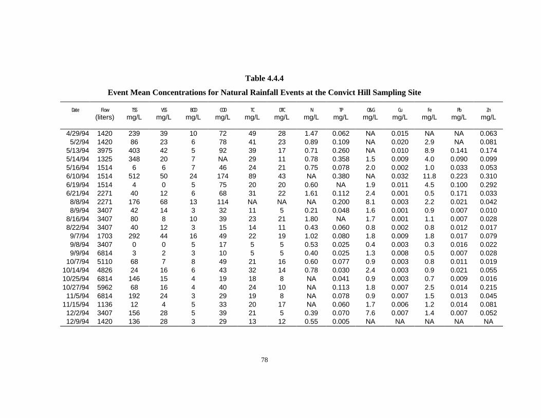
78
Table 4.4.4
Event Mean Concentrations for Natural Rainfall Events at the Convict Hill Sampling Site
Date Flow TSS VSS BOD COD TC DTC N TP O&G Cu Fe Pb Zn(liters) mg/L mg/L mg/L mg/L mg/L mg/L mg/L mg/L mg/L mg/L mg/L mg/L mg/L
4/29/94 1420 239 39 10 72 49 28 1.47 0.062 NA 0.015 NA NA 0.0635/2/94 1420 86 23 6 78 41 23 0.89 0.109 NA 0.020 2.9 NA 0.081
5/13/94 3975 403 42 5 92 39 17 0.71 0.260 NA 0.010 8.9 0.141 0.1745/14/94 1325 348 20 7 NA 29 11 0.78 0.358 1.5 0.009 4.0 0.090 0.0995/16/94 1514 6 6 7 46 24 21 0.75 0.078 2.0 0.002 1.0 0.033 0.0536/10/94 1514 512 50 24 174 89 43 NA 0.380 NA 0.032 11.8 0.223 0.3106/19/94 1514 4 0 5 75 20 20 0.60 NA 1.9 0.011 4.5 0.100 0.2926/21/94 2271 40 12 6 68 31 22 1.61 0.112 2.4 0.001 0.5 0.171 0.0338/8/94 2271 176 68 13 114 NA NA NA 0.200 8.1 0.003 2.2 0.021 0.0428/9/94 3407 42 14 3 32 11 5 0.21 0.048 1.6 0.001 0.9 0.007 0.010
8/16/94 3407 80 8 10 39 23 21 1.80 NA 1.7 0.001 1.1 0.007 0.0288/22/94 3407 40 12 3 15 14 11 0.43 0.060 0.8 0.002 0.8 0.012 0.0179/7/94 1703 292 44 16 49 22 19 1.02 0.080 1.8 0.009 1.8 0.017 0.0799/8/94 3407 0 0 5 17 5 5 0.53 0.025 0.4 0.003 0.3 0.016 0.0229/9/94 6814 3 2 3 10 5 5 0.40 0.025 1.3 0.008 0.5 0.007 0.028
10/7/94 5110 68 7 8 49 21 16 0.60 0.077 0.9 0.003 0.8 0.011 0.01910/14/94 4826 24 16 6 43 32 14 0.78 0.030 2.4 0.003 0.9 0.021 0.05510/25/94 6814 146 15 4 19 18 8 NA 0.041 0.9 0.003 0.7 0.009 0.01610/27/94 5962 68 16 4 40 24 10 NA 0.113 1.8 0.007 2.5 0.014 0.21511/5/94 6814 192 24 3 29 19 8 NA 0.078 0.9 0.007 1.5 0.013 0.045
11/15/94 1136 12 4 5 33 20 17 NA 0.060 1.7 0.006 1.2 0.014 0.08112/2/94 3407 156 28 5 39 21 5 0.39 0.070 7.6 0.007 1.4 0.007 0.05212/9/94 1420 136 28 3 29 13 12 0.55 0.005 NA NA NA NA NA

79
Table 4.4.5
Median Event Mean Concentrations (mg/L)West 35th St.
TrafficSimulation*
West 35th St.No-Traffic
Simulation*
West 35th St.NaturalEvent
Convict HillNatural Event
TSS 291 (0.4) 67 (0.5) 157 (0.9) 83 (1.1)VSS 33 (0.4) 6 (0.5) 42 (0.6) 16 (0.9)BOD5 4.7 (0.8) 2.1 (0.0) 15.3 (0.7) 5.4 (0.8)COD 86 (0.3) 24 (0.2) 142 (0.6) 44 (1.0)Total Carbon 51 (0.4) 14 (0.02) 57 (0.6) 22 (0.7)Dis. Total Carbon 18 (0.6) 13 (0.1) 28 (0.7) 16 (0.6)Nitrate 0.74 (0.3) 0.56 (0.2) 1.00 (0.8) 0.73 (0.6)Total Phosphorus 0.28 (0.5) 0.08 (0.1) 0.41 (0.5) 0.08 (1.0)Oil & Grease 3.7 (0.3) 0.4 (1.7) 5 (1.2) 2 (1.0)Copper 0.022 (0.5) 0.009 (0.03) 0.049 (0.6) 0.006 (1.0)Iron 4.2 (0.3) 1.2 (0.2) 3.5 (0.8) 1.4 (1.2)Lead 0.082 (0.6) 0.023 (1.1) 0.123 (0.8) 0.016 (1.3)Zinc 0.16 (0.8) 0.050 (0.4) 0.263 (0.7) 0.053 (1.1)
* West 35th St. simulation data has been corrected for the background in Austin tap water; Number in parenthesis is the coefficient of variation.
parentheses. The relative variation for most constituents is less during the simulated
events than during natural events. This phenomenon is a result of the “steady-state”
nature (e.g., a constant rainfall, runoff, and traffic rate) of the simulated rain storm. The
similar event duration and sampling protocols among the simulated storms also
contributed to the lower variations observed in the simulated EMCs.
The EMCs for natural storm events are higher than the simulated storm event
EMC values for every constituent except TSS. These results are attributed to a lack of
adequate sampling coverage over the entire duration of most of the natural storm events.
The automatic sampler was programmed with a predetermined sampling sequence to
sample the duration of the expected storm. However, if the rainfall intensity is higher
than anticipated, only the first part of the storm is sampled. Concentrations of
constituents were observed to be higher in the earlier stages of the runoff event, and in
particular during the rising leg of the hydrograph, for all of the constituents under study.
The values for natural storm EMCs would have been smaller had the entirety of each
natural storm been sampled. Likewise, sample collection during the simulated events
always lasted the entirety of the simulated storm event.

80
The higher concentrations of TSS observed during the simulated events are
explained by the intensity of the simulated rainfall. The simulated storms were, on
average, a higher intensity rainfall than the natural storms. The higher flow rates
associated with the simulated events moved more of the heavier dirt particles than the
smaller natural storms.
4.5 Constituent Wash-Off Patterns
The wash-off patterns observed during the simulated storm events for TSS,
nitrate, and oil and grease are shown graphically in Figures 4.5.1a-c, 4.5.2a-c, and 4.5.3a-
c, respectively. Part A of these figures shows the variation in the concentration of the
constituents during the simulated storm events. A period of high concentration is evident
at the beginning of the storm for each constituent. The period of high concentration,
however, occurs simultaneously with the rising leg of the hydrograph and ends at the
time of concentration for the watershed. It is difficult to ascertain from the graph if the
high concentration in the beginning of the storm results from a large amount of material
being washed from the highway early in the storm event (e.g., a true first flush) or from
the smaller volume of water on the watershed at the start of the storm.
The loads for TSS, nitrate, and oil and grease observed during the simulated
events are shown in Figures 4.5.1b, 4.5.2b, and 4.5.3b, respectively. These plots indicate
that load increases linearly with increased flow volume for each constituent as long as
there is traffic to provide an input of constituent mass. The cumulative load curve
becomes relatively flat for the no-traffic simulations, which is a result of the lack of
constituent mass in the runoff. The single exception is nitrate. The cumulative load
curve for nitrate continues to increase even under no-traffic conditions. This
phenomenon is explained by (1) the mobility of nitrate, because of its anionic form
(NO3), does not require the energy associated with vehicles (i.e., the forces resulting from
tires and vehicle-induced winds) to mobilize in the runoff and (2) the amount of nitrates
in the tap water used for the rainfall simulations.

81
TSS
0
200
400
600
800
1000
0 20000 40000 60000 80000Cumulative Flow (liters)
Co
nce
ntr
atio
n (
mg
/l)
Traffic No-Traff ic
(a) Median TSS Concentration During a Simulated Storm Event
TSS
0
1
2
3
4
5
0 20000 40000 60000 80000Cumulative Flow (liters)
Lo
ad (
g/m
)
Traffic No-Traff ic
(b) Median TSS Load During a Simulated Storm Event
TSS
0
2
4
6
8
10
12
0 20000 40000 60000 80000 100000Cumulative Flow (liters)
Lo
ad (
g/m
)
Simulated Natural
(c) TSS Load During Natural and Simulated Storm Events
Figure 4.5.1

82
Nitrate
0
0.2
0.4
0.6
0.8
1
1.2
0 20000 40000 60000 80000Cumulative Flow (liters)
Co
nce
ntr
atio
n (
mg
/l)
Traffic No-Traff ic
(a) Median Nitrate Concentration During a Simulated Storm Event
Nitrate
0
0.002
0.004
0.006
0.008
0.01
0.012
0.014
0 20000 40000 60000 80000Cumulative Flow (liters)
Lo
ad (
g/m
)
Traffic No-Traff ic
(b) Median Nitrate Load During a Simulated Storm Event
Nitrate
0
0.005
0.01
0.015
0.02
0.025
0 20000 40000 60000 80000 100000Cumulative Flow (liters)
Lo
ad (
g/m
)
Simulated Natural
(c) Nitrate Load During Natural and Simulated Storm Events
Figure 4.5.2

83
O&G
00.5
1
1.52
2.53
3.54
0 20000 40000 60000 80000Cumulative Flow (liters)
Co
nce
ntr
atio
n (
mg
/l)
Traffic No-Traff ic
(a) Median Oil and Grease Concentration During a Simulated Storm Event
O&G
0
0.01
0.02
0.03
0.04
0.05
0.06
0 20000 40000 60000 80000Cumulative Flow (liters)
Lo
ad (
g/m
)
Traffic No-Traff ic
(b) Median Oil and Grease Load During a Simulated Storm Event
O&G
0
0.02
0.04
0.06
0.08
0.1
0 20000 40000 60000 80000 100000Cumulative Flow (liters)
Lo
ad (
g/m
)
Simulated Natural
(c) Oil and Grease Load During Natural and Simulated Storm Events
Figure 4.5.3

84
A plot of the total observed load in relation to the total volume of flow is shown
in Figures 4.5.1c, 4.5.2c, and 4.5.3c for TSS, nitrate, and oil and grease, respectively.
Observations for both natural events and simulated events are plotted. No statistical
difference was found between the data observed for simulated events and the natural
events; this is visually evident from the graphs.
The wash-off patterns for all highway runoff constituents are presented in
Appendix F.
4.6 First Flush
The “first flush” of constituents in highway runoff is examined in Figures 4.6.1a-c
and 4.6.2a-c. The percent of the total storm load in relation to the percent of the total
storm flow is shown in Figure 4.6.1a-c. First flush of constituent mass is not strongly
pronounced on pavements with high speed traffic. The percentage of total mass
discharged is only slightly higher than the percentage of the total runoff volume
discharged. The results of Figure 4.6.1a-c are shown numerically in Table 4.6.1.
The fraction of percent mass discharged to percent runoff discharged is plotted in
relation to storm volume in Figure 4.6.2a-c. A value of one indicates the percentage of
the total storm load that has passed is equal to the percentage of the total volume of storm
flow that has passed. The value of this fraction rapidly approaches one and becomes
approximately equal to one shortly after the half-way point in the storm.
4.7 Daily and Seasonal Variations
There is no evidence that any constituents exhibited daily or seasonal trends. A
time-series plot of the TSS and nitrate data collected during the period July 1993 through
July 1994 is presented in Figure 4.7.1. The variation during the day for TSS and nitrate
for the same time period is plotted in Figure 4.7.2.
4.8 Street Sweeping Variations
Street sweeping operations were suspended at the West 35th Street sampling site
during the first 7 months of the study period, and resumed during the last months of the

85
0%
25%
50%
75%
100%
0% 25% 50% 75% 100%Total Flow
To
tal L
oad
TSS
VSS
Nitrate
TP
(a) Load vs. Flow for Solids and Nutrients
0%
25%
50%
75%
100%
0% 25% 50% 75% 100%Total Flow
To
tal L
oad
BOD
COD
TC
DTC
O&G
(b) Load vs. Flow for Organics and Oil and Grease
0%
20%
40%
60%
80%
100%
0% 20% 40% 60% 80% 100%
Total Flow
To
tal L
oad
Cu
Fe
Pb
Zn
(c) Load vs. Flow for Metals
Figure 4.6.1

86
0
1
2
3
4
5
0% 25% 50% 75% 100%Total Flow
(% o
f L
oad
) / (
% o
f F
low
)
TSS VSS Nitrate TP
(a) Percent Load vs. Flow for Solids and Nutrients
02
46
810
1214
16
0% 25% 50% 75% 100%
Total Flow
(% o
f L
oad
) / (
% o
f F
low
)
BOD COD TC DTC O&G
(b) Percent Load vs. Flow for Organics and Oil and Grease
0.0
2.0
4.0
6.0
8.0
10.0
0% 20% 40% 60% 80% 100%
Total Flow
(% o
f L
oad
)/(%
of
Flo
w)
Cu Fe Pb Zn
(c) Percent Load vs. Flow for Metals
Figure 4.6.2

87
Table 4.6.1 First Flush of Highway Runoff Constituents(percentage of constituent load versus percentage of total runoff*)
Traffic Conditions
Total Storm Runoff = 21 mm
No-Traffic Conditions
Total Storm Runoff = 28 mm
% of RunoffVolume of Runoff
21%(4.3 mm)
53%(11.2 mm)
75%(15.7 mm)
19%(5.3 mm)
53%(15.0mm)
75%(21.1 mm)
TSS 27% 55% 74% 42% 75% 87%VSS 28% 52% 76% 44% 65% 73%BOD5 63% 90% 97% 100% 100% 100%COD 32% 59% 76% 51% 93% 95%Total Carbon 27% 60% 79% 45% 72% 90%Dis. Total Carbon 36% 66% 85% 31% 59% 79%Nitrate 25% 56% 74% 31% 62% 83%Phosphorus 29% 61% 82% 63% 82% 94%Oil and Grease 21% 56% 78% 33% 60% 73%Copper 29% 55% 80% 70% 74% 74%Iron 26% 52% 75% 80% 96% 98%Lead 29% 55% 75% 84% 96% 96%Zinc 37% 57% 75% 56% 85% 93%
* Based on the median of all loads and flows recorded during the simulated storm events.

88
TSS
0
2
4
6
8
10
12
Jul-93 Sep-93 Nov-93 Feb-94 Apr-94 Jul-94
Date
Lo
ad (
g/m
)
Simulated Natural
(a) Seasonal Variation (July 1993 - July 1994), TSS
Nitrate
0.000
0.005
0.010
0.015
0.020
0.025
Jul-93 Sep-93 Nov-93 Feb-94 Apr-94 Jul-94Date
Lo
ad (
g/m
)
Simulated Natural
(b) Seasonal Variation (July 1993 - July 1994), Nitrate
Figure 4.7.1

89
TSS
0
2
4
6
8
10
12
12:00 AM 4:48 AM 9:36 AM 2:24 PM 7:12 PM 12:00 AMTime of Day
Lo
ad (
g/m
)
Simulated Natural
(a) Hourly Variation (July 1993 - July 1994), TSS
Nitrate
0.000
0.005
0.010
0.015
0.020
0.025
12:00 AM 4:48 AM 9:36 AM 2:24 PM 7:12 PM 12:00 AMTime of Day
Lo
ad (
g/m
)
Simulated Natural
(b) Hourly Variation (July 1993 - July 1994), Nitrate
Figure 4.7.2

90
study at a sweeping frequency of once every 2 weeks. There were a total of 18 simulated
storm events and 11 natural events sampled during the no-sweep period. Fourteen
simulated events and 12 natural events were sampled during the sweeping period. Two
of the three no-traffic simulated events were conducted during the no-sweeping period.
Using the simulated data only, the median load for the no-sweep period was
compared to the median load for the sweeping period for each constituent. Statistical
difference between the two groups was determined using a t-test. The only constituents
that showed a significant difference between the sweeping periods were the solids. The
storm water loading of both TSS and VSS was reduced as a result of sweeping once
every 2 weeks. The computed values the t-statistic are shown in Table 4.8.1. A negative
sign in front of the t-statistic in Table 4.8.1 indicates that the median load of the
constituent increased during the sweeping period. However, no constituent showed a
significant increase during the sweeping period.
Table 4.8.1 Computed Street Sweeping t-Statistics
Constituent Computed t-Statistic
TSS 3.53(a)
VSS 2.19(b)
BOD5 0.01COD 1.14Total Carbon 1.57Dissolved Total Carbon 1.58Nitrate -1.29Total Phosphorus 1.80Oil and Grease -0.91Copper 0.43Iron -0.79Lead -1.40Zinc 1.80
(a) |t| > t0.01,∞ = 2.326; (b) |t| > t0.05, ∞ = 1.960
4.9 Summary
A total of 35 simulated rainfall events and 23 natural storm events were sampled
at the West 35th Street sampling site. The distribution of EMCs at this site were
positively skewed; however, the degree of skewness was not enough to justify the use of
lognormal estimators to calculate the sample parameters.

91
Constituent wash-off patterns during the simulated events were similar to those
predicted by the wash-off theory presented in Chapter 2. A first flush of constituent mass
was evident during all simulated events; however, it was much more pronounced during
the no-traffic simulations because of the absence of the traffic input.
A street sweeping frequency of once every 2 weeks was found to significantly
reduce the loading of solids (TSS and VSS) in the highway runoff. Street sweeping did
not significantly change the loading of other constituents.

92

93
5.0 Model Development
5.1 Introduction
Predictive modeling of storm water quality is used to provide insight and analysis
into the control of storm water constituents. Storm water models range from simple
screening equations that can be solved on a hand-held calculator to complex simulation
methods that require considerable computer time to complete. The three most common
types of storm water predictive models include regression models, statistical techniques,
and deterministic simulation models.
The regression model is a mathematical equation that defines the line of average
relationship between a dependent variable and one or more independent, or causal,
variables. Storm water regression models commonly identify constituent concentration
or load as variables that are dependent upon runoff volume, rainfall intensity, traffic
intensity, antecedent dry period, surrounding land use, etc. The mathematical approach
used to formulate the regression model is the method of least squares. The method of
least squares minimizes the sum of the squared differences, or residuals, between the
values predicted by the regression equation and the observations. If correctly specified,
the method least squares will provide the best linear and unbiased estimate of the
population parameters.
Regression equations are easy to use and provide a quick method for screening
storm water quality. The storm water regression model can be formulated to predict total
storm load and inner-event loads. Regression models especially are well suited for
predicting the cumulative constituent load that results from a continuous series of storm
events. Regression models have been criticized as poor predictors when applied beyond
the original data set or region from that they were created (Driscoll et al., 1990);
however, this statement is universally true of all water quality modeling methods. Site-
specific quality data is critical for the calibration and verification of urban runoff quality
simulation models (Huber, 1986).
The National Urban Runoff Program (NURP) employed a statistical method for
storm water quality modeling (Driscoll et al., 1990). The NURP statistical method is
based on the assumption that rainfall, runoff volumes, and runoff event mean

94
concentrations (EMC) are all independent, random variables that vary between storm
events. The NURP study concluded that EMCs are random variables that are best
described by a lognormal distribution (USEPA, 1983). Rainfall data historically have
been considered to be represented by a gamma distribution (Chow et al., 1988).
The storm event is assumed to be independent of previous events if the time span
between event midpoints is greater than some minimum time period. This minimum
inter-event time (MIT) is typically in the range of 3 to 24 hours. The MIT is selected by
making use of the assumption that MITs are exponentially distributed (Chow et al., 1988)
and therefore have a coefficient of variation (COV) equal to one. Trial values of the MIT
are chosen until the COV of the time between event midpoints in equal to one (Driscoll
et. al., 1990).
Runoff volumes are calculated using rainfall and runoff statistics. The mean
runoff volume is computed by multiplying the mean volume of a rainfall event by the
ratio of average runoff to rainfall. The mean constituent load is determined by
multiplying the mean EMC by the mean runoff volume (Eq. 3.8.2). All variation in the
constituent loads is assumed to be attributable to the variation in the runoff volume.
The NURP statistical method is relatively easy to apply and can provide a quick
screening like regression equations. The method has also been successfully applied as
part of the NURP program. A shortcoming to the method is that temporal changes in
concentration or load cannot be predicted during the storm. Therefore, the method has
limited use in the evaluation of highway runoff control structures.
Physically based deterministic simulation models represent the most complex
tools available for storm water analysis. Modern computers allow these models to time-
step through the build-up and wash-off of highway constituents, as well as the change in
runoff quantity and quality throughout a drainage system, including storage and treatment
facilities. Most simulation models are capable of performing both single and continuous
event simulations. Build-up and wash-off functions are used to determine the amount of
material removed from the highway surface, and either the nonlinear reservoir method or
kinematic wave method is used to route the runoff throughout the remainder of the
drainage system. Several of the more common simulation models include:
1. Storm Water Management Model (SWMM)

95
2. FHWA Urban Highway Storm Drainage Model
3. Storage, Treatment, Overflow, Runoff Model (STORM)
4. Hydrological Simulation Program - FORTRAN (HSPF)
These models are considered “operational” water quality models and each one has (1) a
user's manual and documentation, (2) is in use by someone other than the model
developer, and (3) has continued support (Huber, 1986).
Simulation models typically consider constituent build-up as a function of the
length of the antecedent dry period and consider constituent wash-off as a function of the
storm duration. Linear equations are sometimes used to describe specific regions of
correlation, but intuition suggests that neither build-up nor wash-off should be entirely
linear. The most common curve forms used to describe constituent build-up are power,
exponential, and Michaelis-Menton expressions. Wash-off curves are generally a
variation of the first-order decay formulation (Huber, 1986). However, a special case of
the regression equation known as a rating curve is also used to describe wash-off. The
rating curve expresses the relationship between load or concentration and flow rate.
Rating curves are almost always power functions, although other forms are sometimes
used (Huber, 1986). Runoff flow routing downstream of the highway pavement is
accomplished using the nonlinear reservoir method or the kinematic wave method.
Simulation models have been designed to model extensive storm water collection
and transfer systems. The models are best applied to urban storm sewer designs that
include extensive pipelines, channels, storage elements, treatment elements, etc.
Simulation models produce the most varied output of any of the modeling methods and
provide the detailed analysis required for the extensive evaluation of comprehensive
storm water controls.

96
5.2 Selection of an Appropriate Modeling Technique
The selection of a storm water quality modeling technique must consider the
objective of the task at hand. The objective of this research is the development of a
model that predicts the amount of material that is washed from the highway surface
during either a design storm event or a design series of storm events. The model output is
the predicted constituent load at the edge of the pavement, at any point during the storm.
All three of the previously mentioned modeling techniques can accomplish this goal;
however, there are several important factors that must be considered in model selection.
The model should be applicable to both single-event and continuous-event design
scenarios. The model should be capable of producing a single storm event loadograph
for the evaluation of the effectiveness of storm water controls. However, receiving
waters respond relatively slowly to constituent inputs. The total load input over an
extended period of time (i.e., weeks to years) is required to estimate response of receiving
waters. All three modeling techniques are capable of single-event and continuous-event
modeling.
The modeling technique also must be capable of estimating the cumulative
amount of load produced at any specific instance during the storm. The ability to predict
cumulative edge-of-pavement loads throughout the storm is an important aspect if the
model is to be used to evaluate control structure efficiency. The amount of constituent
mass captured by a fixed-capacity control structure will be the amount of mass that has
washed from the highway at the time the structure is filled. Subsequently, the amount of
constituent mass released to the receiving stream will be that portion that is washed from
the highway after the structure is full. As shown by the data presented in Chapter 4, the
amount of constituent that is washed from the highway surface varies throughout the
duration of the storm (Figures 4.6.1 and 4.6.2). The concentration of the constituent will
be greater early in the storm than later due of the effect of “first-flush.” The model must
therefore predict the fraction of constituent mass captured by the control structure and the
mass of constituent released by the control structure based on load rate variations during
the storm. Both regression models and physically-based deterministic simulation models
can accomplish this task. However, this condition eliminates the NURP statistical
technique from consideration.

97
A final consideration is the amount of information that the model uses to
determine constituent loading. The more commonly used simulation models (e.g.,
SWMM) determine constituent build-up in terms of elapsed time since the last cleaning
(either by rain or sweeping). Although the available build-up functions include linear,
power, exponential, and Michaelis-Menton, the only information utilized by the model is
the duration of the dry period. The best fit of an exponential function to the TSS data
collected during sampling at the 35th Street site is presented in Figure 5.2.1. The
correlation coefficient (R2 = 0.0013) in Figure 5.2.1 suggests that there are other variables
that influence the build-up of TSS. If the dry period duration was calculated from a
continuous rainfall record, other known variables would include the intensity of the
preceding storm. This new information will indicate the extent of the previous wash-off
and subsequently the amount of residual material remaining on the highway from the
previous storm event. The improved explanatory power that results from using both dry
period duration and previous storm intensity to predict TSS loading at the West 35th
street site is illustrated in Figure 5.2.2
y = 4.3336e0.0001x
R2 = 0.0013
0
2
4
6
8
10
12
0 50 100 150 200 250 300 350
Antecedent Dry Period (hrs)
TS
S L
oad
(g
/m2 )
Figure 5.2.1 Exponential Function Fit to the Data Collected at the West 35th St.Sampling Site

98
0
2
4
6
8
10
12
0 2 4 6 8 10 12
Observed TSS Load (g/m2)
Pre
dic
ted
TS
S L
oad
(g
/m)
R2 = 0.39
Figure 5.2.2 Observed TSS Load vs. Predicted TSS Load using Durationof the Antecedent Dry Period and the Intensity
of the Preceding Storm as Causal Variables
Regression analysis can determine the relationship between numerous causal
variables and the constituent load. Regression analysis will also indicate the statistical
significance of each causal variable as it relates to a specific constituent, which in turn
may suggest possible mitigation procedures or model applicability scenarios.
Furthermore, the formulated regression equation may be used as input to a physically
based deterministic simulation that might model a much broader system.
In summary, regression analysis was chosen as the modeling technique best-
suited for edge-of-the-pavement load calculations because of the following:
• Regression equations can be used to calculate both single-event andcontinuous storm loading patterns.
• Regression models make use of multiple causal variables (e.g., runoffintensity, traffic volume, duration of the dry period, etc.).
• The regression analysis will evaluate the statistical significance of all causalvariables in relation to a specific constituent. This information can suggestmitigation procedures or model applicability situations.
• The regression model can be attached as the input to a larger model simulatinga much broader system.
99
5.3 Identification of Relevant Model Variables
The most important step in the development of an empirical model is the
identification of the relevant explanatory variables. The term “relevant” has two distinct
meanings in regression analysis: scientific relevance and statistical relevance (Johnson et
al., 1987). Scientific relevance is based on the underlying theory guiding the process.
Variables are included in the model because scientific theory suggests inclusion.
Statistical relevance is based on hypothesis tests that suggest whether a coefficient is
“statistically” different from zero. This section describes the process that is used to
identify the set of relevant highway storm water quality causal variables. Note that it
may not be necessary, nor desirable, to use all of the relevant variables in the final storm
water model. The process of selecting the “model variables” from the identified set of
“relevant variables” is discussed Section 5.7.
The mass of constituent that is washed from the highway surface during a storm
event is related positively to the total volume of runoff (Eq. 3.7.2). Scientific theory
suggests that a regression of constituent load against storm runoff will result in the sign
of the runoff coefficient being positive. Furthermore, the computed t-ratio for the runoff
coefficient should be greater than the critical t-ratio at the 0.95 level, which suggests
statistically a 95% confidence level in any decision to reject the null hypothesis that the
runoff coefficient is actually equal to zero. It is possible for scientific theory to suggest
variable relevancy yet be contradicted by statistics, which is the case when the exclusion
of a relevant variable from the model has led to a bias in the statistical analysis.
Likewise, statistical relevance can be established between variables that are correlated
only by happenstance. These inconsistencies make it difficult to distinguish between the
truly relevant explanatory variables and those with only circumstantial correlation. There
are certain traits, however, that are exhibited by all relevant explanatory variables. These
traits include:
(1) some underlying scientific theory explains the response of the dependentvariable to a change in the independent variable;
(2) the variable, when included with all of the other independent variables,must add some explanatory information to the model (i.e., the variablecannot be perfectly collinear with any other variable);

100
(3) the variable is known with certainty or at least capable of being measuredwith a high degree of accuracy.
The process of identifying relevant variables must be based on scientific theory,
otherwise there is no way to distinguish between true causation and circumstantial
correlation. A detailed discussion of correlation and causation is reserved for Section 5.5.
It should be noted here that a high degree of correlation between two variables in no way
implies causation. There is a high degree of correlation, for example, between the yearly
number of publications by Professor Sydney Chapman and the yearly means of sunspot
relative numbers for the years 1910 through 1967 (Campbell, 1968). This correlation is
curious, especially considering that Dr. Chapman worked in fields of research related to
solar changes, but there is absolutely no evidence of causation. The correlation
coefficient is only a measure of the degree of covariation between Dr. Chapman’s
productivity and the sunspot cycle and nothing more. The correlation coefficient, or the
more commonly used square of the correlation coefficient (R2), is a measure of the
“explanatory” power of the regression equation only if the variables that are selected for
use in the regression are derived from some guiding theory that bestows the equation with
causality.
A variable that is “relevant” also must add explanatory information that is
independent of the information collectively added by all other relevant variables in the
model. The “independence” of the explanatory variable must be considered in the
selection process because many variables in the storm water runoff process tend to move
together. The size of a storm event, for example, may be expressed in terms of rainfall
volume, runoff volume, duration of the storm, or the number of vehicles that traveled
through the storm. The lack of independent movement among the explanatory variables
is a condition known as multicollinearity.
Multicollinearity affects every storm water runoff data set. A precise estimate of
the effect of single variable is difficult since all of the variables move together. This
results in is high values for the variance of the estimated coefficients which increases the
standard error of the regression and reduces the t-ratio. A small t-ratio is not necessarily
a problem as long as the analyst is not mislead by a small t-ratio that is the result of the
presence of multicollinearity. However, multicollinearity causes the statistical

101
significance of the computed variable coefficient to vary depending on what other
variables happen to be present in the equation. This situation is interpreted as
“instability” in the regression coefficients. Scientific theory provides only general
guidelines for the selection of specific empirical variables (e.g., a general mass balance
says that the amount of material contained in the output of a storm water system is
determined by the amount of material input into the system, plus or minus any decay or
production of the material within the system; the mass balance does not indicate what the
specific inputs might be for a particular system); therefore, it is customary when working
with highway runoff data to experiment with alternative specifications of the same basic
equation. A number of formulations of the runoff model are developed that differ only
by the specific causal variables used, such as storm duration, rainfall volume, runoff
volume, traffic during the storm, duration of the antecedent dry period, traffic during the
dry period, etc. A correlation among the variables in the sample exists; therefore, the
coefficients of some variables will be significant in some formulations and not significant
in others. The coefficients will appear to be “unstable” under these conditions.
Multicollinearity does not effect the predictive performance of a regression
equation (Anselmi, 1987). The reason is that multicollinearity only obscures the
individual effects of each explanatory variable on the dependent variable. The regression
results will remain valid in terms of the effects on the dependent variable by the
collective action of the explanatory variables as long as the conditions that originally
caused the multicollinearity remain constant.
A perfect correlation between variables is seldom the case in storm water data
sets, if for no other reason than measurement error. However, perfect correlation may
occur, if the regression model is used to predict storm loading. For example, if the
predictive model uses both rainfall volume and runoff volume as explanatory variables,
and rainfall totals are the only data available, the user of the model would have to
estimate runoff as a function of rainfall. Runoff volume, in this case, would be perfectly
correlated to rainfall volume and would therefore not add any new information to the
model.
A trait of a relevant variable is measurability. The regression equation assumes
that there is measurement error associated with the value of the dependent variable. This

102
error is one of the primary reasons for the existence of a disturbance term associated with
each regression equation (refer to Appendix G). However, the regression assumes that
there is no measurement error in the independent variables. Any measurement error on
the right-hand side of the equation will invalidate the regression. Therefore, any variable
selected for use as an independent variable in the model should be one that is known or
can be measured with certainty. For example, consider the variables total rainfall and
total runoff. If there is no variation in the rainfall over the highway watershed, which is a
reasonable assumption for short highway watersheds between curb inlets, the total
rainfall can be measured more accurately than the total runoff from the watershed. All
other factors equal, total rainfall would make a better explanatory variable than total
runoff.
In summary, ordinary least squares regression will determine the correlation
between any two variables, but sound scientific principles determine if the response of
one variable is truly attributable to a change in another. Once a variable is determined to
have scientific significance, other factors such as multicollinearity and measurability
should be considered in order to establish the relevancy of the variable. The final
variables used in the model are selected using statistical procedures outlined in Section
5.7.
The causal variables that influence constituent loading in highway storm water
runoff were determined to originate during three different time periods: (1) the current
storm, (2) the antecedent dry period, and (3) the preceding storm. Mathematically, the
general population regression equation is given as:
Y X X Xs s s s si si= + + + +β β β β0 1 1 2 2( ... )+ + + +( ... )β β βa a a a ai aiX X X1 1 2 2
+ + + +( ... )β β βp p p p pi piX X X1 1 2 2
+ U i (5.3.1)where the subscripts s, a, and p refer to variables from the storm, the antecedent dry
period, and the preceding storm respectively, and U is the uncertainty term. Table 5.3.1
lists the relevant variables identified during this study.

103
Table 5.3.1 Relevant Model Variables
Variable Example of Effect
Date of the Storm Seasonal trendsTime of Day of the Storm Atmospheric conditions may change during periods
of industrial activityStorm Duration Potential for further constituent inputTotal Rainfall or Total Runoff Directly related to constituent loadingIntensity of Runoff Higher kinetic energy in runoff may flush more
materialTraffic Count during the Storm Traffic is the source of certain constituentsTraffic Mix during the Storm Construction vehicles, diesel-powered vehicles, and
others may be “dirtier” than the normal population of vehicles
Traffic Speed during the Storm Scour from tires and vehicle-induced wind forces increase with speed
Surrounding Land Use Industrial areas are “dirtier” than rural areasCurb / Guardrail Height Taller guardrails trap constituents along the highwayDuration of Antecedent Dry
PeriodProvides the opportunity for the build-up of
constituentsAntecedent Traffic Count Increased opportunity for dry vehicle contributionsWeather Conditions Heavy winds during the dry period could remove
constituents from the highway surfaceMaintenance Activities Grass cutting, bridge sanding, and guardrail
maintenance add dirt and debris to the highway surface
Street Sweeping Potential to remove constituents from highway surface
Previous Storm Characteristics The degree of removal during the previous storm event will affect the amount of material available for the current storm event.
5.4 Worksheet Development
The worksheet is a systematic way to organize and record the values of all
variables used in the regression analysis. The columns of the worksheet identify the
variables that are used in the analysis, and the rows contain the respective values of the
variables for each observation. This task was accomplished with an Excel spreadsheet,
that is compatible with the MicroTSP Econometric software used for the regression
analysis.

104
The values of all variables for each observation were recorded as cumulative
values from the beginning of the storm event so that each observation could be
considered the end of the current runoff. Therefore, the 450 observations recorded during
the 35 simulated rainfall events and 23 natural storm events each represent an individual
runoff event. The advantages to organizing the data in this manner are (1) an increase in
the available number of storm events for the regression analysis and (2) the regression
equation formulated from the data set will be able to predict inner-event loading patterns.
The disadvantage, however, is the introduction of autocorrelation, into the data set.
Autocorrelation results when the value of a variable is dependent on the preceding value
of the variable. A data set can be transformed, however, to account for the
autocorrelation prior to the formulation of the regression equation. The method used to
transform the data in this research is presented in Appendix G.
The constituent loads are adjusted for background concentrations of the
constituent prior to the formulation of the regression equation. Background
concentrations for the rainfall simulations are the constituent concentrations measured in
the tap water, and background concentrations for the natural storm events are the
constituent concentrations measured in the rainfall. In the worksheet, only the
observations recorded during the rainfall simulations were adjusted for background
concentrations of the constituents. The difference between the constituent concentration
measured in the tap water and the average concentration measured for the constituent in
the natural rainfall was added/subtracted to the constituent concentration measured in the
simulated runoff sample. This method essentially “normalized” the simulated runoff
samples to match the natural runoff samples.
Scaling of the variables is also identified in the worksheet. The objective of the
regression analysis is to formulate a predictive equation that is applicable to highway
watersheds other than the West 35th Street site. Constituent loads recorded in the
worksheet are in units of grams per square meter of highway surface (g/m2) to account
for differences in watershed areas. Likewise, runoff discharge rates were recorded in
liters per minute per square meter of highway surface (l/m2/min). Vehicle counts during
the wet and dry periods were recorded as the average count per lane of traffic in order to
be compatible with watersheds with a different number of traffic lanes.

105
5.5 Covariance, Correlation, and Causation
Covariance is the measure of linear dependence between two variables. The
covariance is given by:
Cov x yx x y y
ni i( , )
( )( )=
− −−
∑1 (5.5.1)
where: xi = ith observation of variable x;
yi = ith observation of variable y;
x = mean of x;
y = mean of y;
n = number of observations.
A large value of covariance indicates a strong linear relationship between two
variables and is equal to zero if the two variables are independent. The covariance also
could equal zero if the two variables are related by a non-linear function such as a
quadratic or exponential. The covariance, however, has little application to highway
storm water quality because the covariance is dependent on the scales chosen for the two
variables. This makes it impossible to know whether the value of the covariance is truly
large or small.
The problem is solved by converting the covariance to a scaleless covariance by
dividing by the standard deviations of the two variables. The scaleless covariance is
called the correlation coefficient, r, and is shown mathematically as:
r x y
x x y y
nS S
i i
x y
( , )
( )( )
=
− −−
∑1
(5.5.2)
where: Sx = standard deviation of x;
Sy = standard deviation of y.
The value of the correlation coefficient ranges from -1 to +1, and values that
approach -1 or +1 indicate a strong correlation between x and y. If the sign of the
correlation coefficient is positive, the value of x increases with an increase in y, and if the
sign is negative, the value of x decreases with an increase in y.

106
The coefficient of multiple determination, or R2, is the square of the correlation
coefficient and is often used in regression analysis to measure the percent of variation in
the dependent variable associated with, or explained by, variation in the independent
variable. The degree of correlation between two variables in no way implies causation.
However, the correlation coefficient can be used to measure the degree of causation if
there is reason to believe the two variables are related in the system under study.
Furthermore, R2 is only a measure of the linear association between two variables. Two
variables may be related according to a nonlinear function and have a low value of R2.
The correlation coefficients between suspected causal variables and highway
runoff constituents are presented in Table 5.5.1.
Table 5.5.1 Correlation Coefficients Between Suspected Causal Variablesand Constituent Load (g/m2)
TSS VSS BOD5 COD TotalCarbon
Dis. TotalCarbon
NO3 TP Oil &Grease
Cu Fe Pb Zn
Duration 0.07 0.05 0.24 0.30 0.07 0.12 0.11 0.31 0.42 0.49 0.12 0.17 0.32Flow 0.91 0.92 0.76 0.87 0.87 0.96 0.94 0.82 0.86 0.59 0.91 0.51 0.67Intensity 0.79 0.79 0.61 0.67 0.72 0.77 0.77 0.64 0.60 0.38 0.74 0.37 0.54VDS 0.15 0.13 0.39 0.43 0.18 0.27 0.25 0.40 0.56 0.40 0.23 0.23 0.40Air Temp. -0.04 0.04 0.14 0.09 -0.07 0.06 0.10 0.14 -0.01 -0.01 0.03 -0.09 0.06ADP 0.14 0.21 0.28 0.16 0.16 0.27 0.31 0.21 0.09 0.06 0.12 0.05 0.22ATC 0.11 0.18 0.28 0.18 0.13 0.25 0.31 0.21 0.09 0.05 0.09 0.03 0.23ADPTemp.
-0.18 -0.12 0.02 -0.03 -0.19 -0.05 0.01 0.00 -0.12 -0.06 -0.12 -0.17 -0.04
P-Duration 0.14 0.16 0.05 -0.16 0.27 0.05 -0.05 -0.10 0.04 0.01 0.17 0.12 -0.12P-Flow 0.11 0.10 0.19 0.16 0.10 0.16 0.22 0.21 0.07 -0.04 0.13 0.05 0.20P-Intensity 0.03 0.03 0.18 0.29 -0.08 0.15 0.27 0.32 0.04 -0.02 0.04 -0.02 0.32P-VDS 0.06 0.12 -0.01 -0.17 0.20 0.01 -0.09 -0.16 -0.01 0.03 0.12 0.10 -0.12P-Temp. -0.30 -0.29 -0.05 -0.07 -0.34 -0.15 -0.07 -0.05 -0.19 -0.12 -0.27 -0.28 -0.12 Duration of storm is in units of minutes; Flow = L/m2; Intensity = volume of runoff / duration; VDS = Vehicle count during the storm; ADP = Duration of the antecedent dry period; ATC = Vehicle count during the antecedent dry period; Temperature in oC; P prefix indicates previous storm characteristic.
5.6 Model Misspecification
There are four assumptions regarding the residuals that must be made for ordinary
least squares (OLS) regression to be valid. The implications of these assumptions and the
remedies used to satisfy misspecifications are discussed in Appendix G. A fifth
assumption, which of multicollinearity, is made when formulating a multiple regression
model. The effects of multicollinearity have been described in Section 5.3.

107
5.7 Variables Included in the Model
Theoretically, all of the variables identified in Table 5.3.1 influence the
constituent load in highway runoff and should be included in any empirical model used to
predict the constituent loading in highway runoff. Unfortunately, it is not possible to
include all of the identified variables in the model, nor is it particularly desirable. Some
of the variables, such as surrounding land use, traffic speed, and traffic mix cannot be
used in the model because their values are fixed in the data set. There are other variables
that influence constituent loading in highway runoff that have not been identified because
of a lack of knowledge of the build-up/wash-off process. Furthermore, the inclusion of
all relevant variables in the model, or model overfitting, can be harmful because the
prediction error of the model is proportional to the number of parameters in the model
(Berthouex and Brown, 1994). The goal is to determine an adequate model with the
fewest possible terms. Unfortunately, the method of selecting the final model is strictly
trial and error and dependent on the subjectivity of the analyst.
A three-phase approach was used to search for the simplest, “adequate” model.
The first phase begins with an overfit of the model. The regression equation is
formulated using every known causal variable and each coefficient is examined for
statistical relevance (a computed t-ratio greater than the critical t-ratio for rejecting the
null hypothesis at the 0.95 level) and scientific relevance (the coefficient has the expected
sign) to determine that variables are candidates for discard. The variables that fail both
tests are eliminated one at a time, the regression equation is reformulated, and the new
coefficients are examined for relevance. The procedure is repeated until there are no
longer any variables that are statistically insignificant and display the wrong sign.
The second phase of the search involves making a judgment on the variables that
show statistical significance and not scientific significance, or vise versa. If the variable
is statistically significant and scientifically relevant, but does not have the expected sign,
it is allowed to remain in the model since the probable cause of the sign change is
multicollinearity with an included or excluded variable. The decision is not as
straightforward if the variable is scientifically relevant and has the expected sign, but is
not statistically significant. In most cases, the variable is eliminated from the model.

108
However, there are some circumstances in which the variable should be allowed to
remain in the model. Multicollinearity may have reduced the value of the computed t-
ratio below the critical t-ratio, which could lead to the wrong conclusion.
The final phase of the search involves a reconsideration of the discarded variables
since scientific theory suggests that all of the variables should be included in the model.
It is possible for a variable that was discarded early in the process to become statistically
relevant in a new model formulation with a fewer number of variables. All discarded
variables, therefore, should be individually reinserted into the trimmed model and tested
for relevance.
The model development included the testing of different functional forms of the
major independent variables. For example, it is not scientifically appealing to use the
duration of the antecedent dry period in a linear form. Intuitively, the build-up of
material on the highway surface is not linear throughout the range of possible dry period
durations, but becomes asymptotic at some level. In this case, it is more appealing to
specify the reciprocal of the dry period duration in the model.
During model development, the linear, reciprocal, and quadratic forms of the
major independent variables were specified in model. The log-log [i.e., Ln(y) = C
+βLn(x)] and linear-log [i.e., y = C + βLn(x)] model forms also were specified.
Interestingly, a linear-linear specification showed the greatest explanatory power for all
constituents in the West 35th Street data.
It is tempting to rank the independent variables in order of their relative
importance during the selection process. Methods used to rank variables include
comparing the magnitudes of the variable coefficients, comparing simple correlation
coefficients, and comparing t-ratios. None of these methods, however, are particularly
attractive.
The absolute values of the coefficients should not be used to make statements
about the relative importance of the variables in the equation. The magnitude of the
coefficient is meaningless since the variables are scaled in different units. Simple
correlation coefficients, such as those in Table 5.5.1, also should not be used to rank the
importance of variables. Correlation coefficients are computed without regard for the
effect on the dependent variable of the other relevant variables in the equation.

109
A third basis for assigning importance to model variables is ranking by the
magnitude of the respective t-ratio. The t-ratio cannot be used to rank variables. If a
variable has a t-ratio that is twice the size of the t-ratio of another variable, it does not
follow that the variable is twice as important. All it suggests is that the relative variance
of one estimated coefficient is smaller than the relative variance of the other. If the
computed t-ratio exceeds the critical t-ratio for the confidence level of the test, all that
can be stated is that the null hypothesis can be rejected.
The methods of beta coefficients and elasticities offer the best possibilities for
ranking model variables. A description of these methods may be found in most texts on
regression analysis including Johnson et al. (1987). However, there are no compelling
reasons to rank the variables of the highway constituent runoff model.
5.8 Summary
The regression model was found to have the most applicability for predicting
edge-of-pavement constituent loads in highway runoff. Regression equations can (1) be
formulated that calculate both single-event and continuous storm loading patterns, (2)
make use of multiple causal variables, (3) provide information that can suggest mitigation
procedures or model applicability situations, and (4) be attached as the input to a larger
model simulating a much broader system.
The model was developed using a three-stage approach to examine the
applicability of suspected causal variables. The goal was to formulate the model with the
fewest explanatory variables in order to reduce prediction error. Because the explanatory
variables selected for use in the model are based on both scientific and statistical
relevance, the calculated correlation coefficient is an effective measure of the explanatory
power of the equation. The linear forms of the explanatory variables were found to have
greater explanatory power than other functional forms such as reciprocal and quadratic.

110

111
6.0 Model Results
6.1 Introduction
The results of the regression equations that were formulated using the data
collected at the West 35th Street sampling site are presented in this chapter. Although
data were collected during both simulated and natural rainfall events, no statistical
difference was detected among the data generated with the rainfall simulator and those
collected during the natural storm events. Therefore, no attempt was made to segregate
simulated from natural data during model formulation. The regression equations were
formulated using the combined data for storm events sampled at the West 35th Street site.
A statistical difference was detected among the street sweeping data. Street
sweeping was not conducted at the West 35th Street during the first 7 months of the study
period, but resumed during the last 5 months of the study at a sweeping frequency of
once every 2 weeks. No significant correlation was detected among the constituent loads
and the amount of time since the street sweeping activity. However, a statistical
difference was detected among the data collected for each period. Therefore, two sets of
regression equations were formulated. The first set applies to highway pavements where
no street sweeping activity occurred and the other to highway pavements that are swept
on a frequency of approximately once every 2 weeks. Examples of each equation are
given in the chapter. The results of all regression analysis are presented in Tables 6.2.1,
6.2.2, and 6.2.3, and in Figures 6.2.1 through 6.2.4. Additional data also are presented in
Appendix I.
6.2 Results of the Regression Analysis
The numerical results of the regression formulation are presented in Tables 6.2.1
and 6.2.2. The first column lists the constituents that were modeled. The second column,
N, is the size of the sample used to formulate the regression. The differences in sample
size among the constituents is mostly a result of missing data. The maximum sample size
possible is 422, which is the result of the 423 observations recorded less 1 observation

112
Table 6.2.1 Summary of Model Coefficients (Non-Metals)
Constituent(g/m2)
N S(g/m2) R2 C Duration
(min)Flow
(L/m2)Intensity
(L/m2min)VDS ADP
(hrs)ATC PDUR
(min)PFLOW(L/m2)
PINT(L/m2min)
TSS 402 0.5482 0.93 0.2556* 0.3068 2.0181 0.0037 -2.9865(0.2721) (0.0140) (0.8077) (0.0007) (0.6989)
VSS 401 0.0630 0.93 -0.0186* 0.0348 0.1649 0.0005 0.0069 -0.6721(0.0322) (0.0016) (0.0932) (0.0001) (0.0013) (0.1336)
COD 420 0.1169 0.95 -0.0613* 0.0007 0.0773 0.7785 -0.0041 6.0E-6(0.0343) (7.8E-5) (0.0025) (0.1156) (0.0009) (1.2E-6)
Phosphorus 411 0.0005 0.90 -0.0005 3.3E-6 0.0002 0.0032 5.1E-9(0.0002) (3.6E-7) (1.1E-5) (0.0005) (8.0E-10)
Nitrate 351 0.0010 0.95 -0.0015 0.0006 0.0086 1.2E-8(0.0004) (2.8E-5) (0.0016) (1.6E-9)
Total Carbon 404 0.0766 0.94 -0.0657* -0.0011 0.0411 0.7307 1.1E-4 6.7E-7(0.0322) (1.6E-4) (0.0015) (0.0965) (1.7E-5) (1.3E-7)
Dis. TC 402 0.0265 0.91 -0.0306 0.0073 0.3585 2.2E-5 1.3E-7 0.1983(0.0108) (0.0005) (0.0324) (2.8E-6) (5.5E-8) (0.0585)
BOD5 398 0.0145 0.86 -0.0081* 0.0035 0.0619 1.1E-5 1.5E-7(0.0046) (0.0004) (0.0228) (1.6E-6) (2.3E-8)
Oil and Grease 263 0.0054 0.94 -0.0004* 0.0030 1.0E-5(0.0020) (8.9E-5) (5.8E-7)
N = # of observations.; S = std. error of regression (g/m2); R2 = correlation coefficient adjusted for degrees of freedom; C = intercept; Duration = duration of storm event (min); Flow = total volume of runoff per unit area of watershed (L/m2); Intensity = Flow divided by Duration (L/m2/min); VDS = single-lane vehicle count during storm; ADP = duration of antecedent dry period (hrs); ATC = single-lane vehicle count during ADP; PDUR = duration of the previous storm event (min); PFLOW = total volume of runoff per unit area of watershed during the previous storm event (L/m2); PINT = PFLOW divided by PDUR (L/m2/min); An asterisk indicates the coefficient is not statistically different from zero; Numbers in parenthesis are the standard error of estimate of the coefficients; Example: TSS (g/m2) = 0.2556 + 0.3068(Flow) + 2.0181(Intensity) + 0.0037(ADP) - 2.9865 (PINT) This table is applicable only to highway pavements with no street sweeping activity. Refer to Table 6.2.3 for street sweeping adjustments.

113
Table 6.2.2 Summary of Model Coefficients (Metals)
Constituent(g/m2)
N S(g/m2) R2 C Duration
(min)Flow
(L/m2)Intensity
(L/m2min)VDS ADP
(hrs)ATC PDUR
(min)PFLOW(L/m2)
PINT(L/m2min)
Iron 399 0.0084 0.92 -0.0028* 0.0042 0.0282 2.3E-5(0.0028) (0.0002) (0.0082) (1.0E-5)
Zinc 399 0.0007 0.92 0.0002* 2.5E-6 0.0001 4.9E-9 -3.2E-6 0.0003 -0.0241(0.0002) (4.2E-7) (7.9E-6) (1.1E-9) (3.0E-7) (1.5E-5) (0.0016)
Lead 319 0.0004 0.68 0.0008 6.5E-5 -0.0020 8.0E-8 -0.0023(0.0002) (8.9E-6) (0.0006) (2.4E-8) (0.0008)
Copper 398 8.1E-5 0.90 1.9E-5* 3.8E-6 2.4E-5 -2.4E-7(2.0E-5) (1.5E-7) (9.6E-7) (1.6E-8)
N = # of observations.; S = std. error of regression (g/m2); R2 = correlation coefficient adjusted for degrees of freedom; C = intercept; Duration = duration of storm event (min); Flow = total volume of runoff per unit area of watershed (L/m2); Intensity = Flow divided by Duration (L/m2/min); VDS = single-lane vehicle count during storm; ADP = duration of antecedent dry period (hrs); ATC = single-lane vehicle count during ADP; PDUR = duration of the previous storm event (min); PFLOW = total volume of runoff per unit area of watershed during the previous storm event (L/m2); PINT = PFLOW divided by PDUR (L/m2/min); An asterisk indicates the coefficient is not statistically different from zero; Numbers in parenthesis are the standard error of estimate of the coefficients; Example: Iron (g/m2) = -0.0028 + 0.0042(Flow) + 0.0282(Intensity) + 0.000023(ADP) This table is applicable only to highway pavements with no street sweeping activity. Refer to Table 6.2.3 for street sweeping adjustments.

114
lost due to the first-order autocorrelation adjustment. The third column, S, is the standard
error of the regression. Ninety-five percent of the regression predictions fall within plus
or minus two standard errors of the regression. The fourth column is the coefficient of
multiple determination, R2, adjusted for degrees of freedom.
The following terms/acronyms are used in Table 6.2.1 to identify the variables
used in the regression equations:
C = the constant (y-intercept) term in the equation;
Duration = total duration of storm in minutes;
Flow = the total volume of flow per unit area of watershed during thestorm (L/m2);
Intensity = Flow divided by Duration (L/m2/min);
VDS = average number of vehicles traveling through the storm in asingle lane;
ADP = total duration of the antecedent dry period in hours;
ATC = average number of vehicles using the highway during the ADPin a single lane;
PDUR = the total duration of the preceding storm in minutes;
PFLOW = the total volume of flow per unit area of watershed (L/m2) thepreceding storm event;
PINT = PFLOW divided by PDUR (L/m2/min)
Columns 5 through 14 of Tables 6.2.1 and 6.2.2 list the coefficients of the
independent variables of the equation. The number in parentheses is the standard error of
the coefficient. A coefficient marked with an asterisk indicates that the coefficient is not
statistically different than zero as determined by the t-statistic (i.e., one cannot be 95%
confident the coefficient is not zero since ± 2 standard errors include zero). The only
coefficients included in the final regression equation that failed the t-test are those of the
y-intercept term C. The combination of high adjusted R2 values with the statistically
significant coefficients indicate that the equations are a “good fit” of the West 35th Street
data (further evidence of a good model fit is the normality of the residuals exhibited in
Appendix H).
The constituents listed in both Tables 6.2.1 and 6.2.2 are listed in ascending order
according to the importance of the traffic count during the storm (VDS) in the regression
equation. For example, the first constituent listed in Table 6.2.1, TSS, has the regression

115
equation comprised of the fewest number of explanatory variables of that VDS is not
included. The last constituent listed, oil and grease, has the regression equation
comprised of the fewest number of explanatory variables of that VDS is included.
Traffic count during the antecedent dry period was considered to be less important than
traffic during the storm in this order system.
The interpretation of Tables 6.2.1 and 6.2.2 is presented below using TSS for an
example. The predictive equation for the edge-of-pavement loading for TSS is
determined using the coefficients shown in line 1 of Table 6.2.1, columns 5 through 14.
The predictive equation for TSS is therefore:
TSS(g/m2) = 0.2556 + 0.3068(Flow) + 2.0181(Intensity)+ 0.0037(ADP) - 2.9865(PINT) (6.2.1)
The positive (+) sign preceding the coefficients of Flow, Intensity, and ADP
indicates that an increase in the value of any of these variables will result in an increase
in the load of TSS. Likewise, the greater the intensity of the preceding storm event
(PINT), the less the TSS load (i.e., there is less material remaining on the highway
following a larger storm event). The values given in parenthesis under each coefficient in
Table 6.2.1 are the standard errors of the coefficients. There is a 95% probability that the
true value of the variable coefficient is within +/- 2 standard errors (the given coefficients
are not necessarily the “true” values since there is uncertainty, or a lack of knowledge,
regarding the underlying build-up and wash-off processes of TSS in nature). For
example, there is a 95% probability that the true value of the coefficient for ADP is
between 0.0023 and 0.0051. Note that if there is no storm event at all (i.e., Flow,
Intensity, ADP, and PINT are all equal to zero), the load of TSS is not equal to zero, but
rather 0.2556 g/m2. However, the standard error for the constant term, C, is 0.2721, and
there is a 95% chance that the true value of the constant term is between -0.2886 and
0.7998. Since this range includes the value of zero, the equation actually states that there
is a 95% probability that the true load of TSS is zero if there is no storm at all.
The TSS equation was formulated from a data set consisting of 402 observations
(shown in column 2 of Table 6.2.1). This information is helpful in determining the
degrees of freedom of the regression analysis (i.e., the number of linear independent
pieces of information in n observations). For example, the TSS regression has 397

116
degrees of freedom, which is the result of 402 (number of observations) less 5 (the
number of estimated parameters, or the coefficients of the three explanatory variables
plus the constant term).
The standard error of the TSS regression is 0.5482 (shown in column 3 of Table
6.2.1). This number is an estimate of the uncertainty (i.e., lack of knowledge) that exists
within the West 35th Street TSS data. During the fit of the West 35th Street TSS data,
95% of the equation predictions were within +/- 1.0964 g/m2 (i.e. two standard errors) of
the observed value. Note that this is not the same as the standard error of the forecast,
which is almost always larger than the standard error of the regression.
The adjusted R2 of the TSS regression is 0.93 (shown in column 4, Table 6.2.1).
This number indicates that 93% of the variation in the TSS loading observed at the West
35th Street sampling site is explained by the variables Flow, Intensity, ADP, and PINT.
Table 6.2.3 gives the set of “street sweeping shifts” determined from the analysis
of the West 35th Street data. These coefficient shifts should be added to the coefficient
values given in Tables 6.2.1 and 6.2.2 if the regression equations are to be used for
highway pavements where street sweeping is performed approximately once every 2
weeks. The following equations demonstrate the use of the street sweeping shifts for
iron:
The predictive model for iron from Table 6.2.2 (i.e., used if there is no sweeping):
Iron(g/m2) = -0.0028 + 0.0042(Flow) + 0.0282(Intensity) + 0.000023(ADP)
The predictive model for iron if there is once every two week sweeping:
Iron(g/m2) = -0.0028 + (0.0042-0.0006)(Flow) + 0.0282(Intensity) + 0.000023(ADP)

117
Table 6.2.3 Street Sweeping Shifts (once every 2 weeks sweeping schedule)
Constituent(g/m2)
C Duration(min)
Flow(L/m2)
Intensity(L/m2min)
VDS ADP(hrs)
ATC PDUR(min)
PFLOW(L/m2)
PINT(L/m2min)
TSS -0.8225 -0.1484 2.6652(0.3031) (0.0190) (1.0463)
VSS -0.0574 -0.0142 0.2724 -0.0003 -0.0034 0.1236(0.0413) (0.0022) (0.1231) (0.0002) (0.0018) (0.2120)
BOD5 -0.0014 0.0728 -7.6E-6(0.0006) (0.0278) (0.0000)
COD -0.0181(0.0023)
Total Carbon 0.0011 -0.6375 -0.0001(0.0002) (0.0877) (1.9E-5)
Dis. Total Carbon -0.2597 -1.5E-5 3.3E-7 -0.1916(0.0302) (2.9E-6) (8.9E-8) (0.0737)
Nitrate 0.0017 0.0002 -0.0096(0.0005) (3.7E-5) (0.0020)
Phosphorus -8.0E-5(1.1E-5)
Oil and Grease -0.0009(0.0002)
Copper -3.5E-6 2.2E-7(2.1E-7) (1.9E-8)
Iron -0.0006(0.0002)
Lead -0.0010 0.0031 0.0028(0.0002) (0.0006) (0.0012)
Zinc 2.7E-6 -0.0003 0.0233(3.7E-7) (2.1E-5) (0.0024)
Shifts should only be used with coefficients in Tables 6.2.1 and 6.2.2. Refer to Tables 6.2.1 and 6.2.2 for acronym descriptions. Example: Iron (g/m2) = -0.0028 + (0.0042 - 0.0006)(Flow) + 0.0282(Intensity) + 0.000023(ADP)

118
The values shown in parentheses in Table 6.2.3 are the standard errors of the
estimates of the sweeping shifts. All of the shifts in Table 6.2.3 have been determined to
be statistically different from zero by using the t-test.
As shown in Table 4.8.1, not all constituent loads were reduced during the period
of street sweeping. The street sweeping shifts reflect these results. The highway runoff
model was used to calculate the expected storm water loading for each constituent during
a design storm under two assumptions: (1) a street sweeping program with a once every 2
weeks schedule was currently being conducted and (2) no street sweeping program was
being conducted. The results are presented in Table 6.2.4. The parameters of the design
storm are footnoted in Table 6.2.4.
The results of the regression analysis are shown graphically in Figures 6.2.1
through 6.2.4 for TSS, COD, nitrate, and zinc, respectively. Similar figures are presented
Table 6.2.4 Expected Loads based on MoPac Street Sweeping Program
Constituent Expected Load withStreet Sweeping
(g/m2)
Expected Loadwithout Street
Sweeping(g/m2)
TSS 3.2 5.8VSS 0.4 0.6BOD5 0.09 0.10COD 1.3 1.6Total Carbon 0.7 1.0Dissolved Total Carbon 0.19 0.29Nitrate 0.014 0.012Total Phosphorus 0.003 0.005Oil and Grease 0.07 0.07Copper 0.0004 0.0004Iron 0.07 0.08Lead 0.0014 0.0007Zinc 0.003 0.001
Storm duration = 60 minutes; Rainfall intensity = 25.4 mm/hr (1 in/hr); Vehicles during the storm = 3,136; Antecedent dry period = 7 days; Traffic count during dry period = 131,396; Previous storm duration = 60 minutes Previous storm intensity = 25.4 mm/hr (1 in/hr); Watershed size = 4358 m2 (46,910 ft2) Traffic lanes = 3

119
-2
0
2
4
6
8
10
12
0 2 4 6 8 10 12
Observed Load (g/m2)
Pre
dic
ted
Lo
ad (
g/m
)
(a) Fit of Data from West 35th Street Site
TSS
-3
-2
-1
0
1
2
3
0 5 10 15 20 25 30 35
Total Rainfall (mm)
Res
idu
al (
g/m
)
(b) Model Residuals vs. Total Rainfall (Dashed Lines Indicate ± 2 Std. Error)
Figure 6.2.1 TSS Model Results

120
-0.5
0
0.5
1
1.5
2
2.5
3
0 0.5 1 1.5 2 2.5 3
Observed Load (g/m2)
Pre
dic
ted
Lo
ad (
g/m
)
(a) Fit of Data from West 35th Street Site
COD
-0.6
-0.4
-0.2
0
0.2
0.4
0.6
0.8
0 5 10 15 20 25 30 35
Total Rainfall (mm)
Res
idu
al (
g/m
)
(b) Model Residuals vs. Total Rainfall (Dashed Lines Indicate ± 2 Std. Error)
Figure 6.2.2 COD Model Results

121
-0.005
0
0.005
0.01
0.015
0.02
0.025
0 0.005 0.01 0.015 0.02 0.025
Observed Load (g/m2)
Pre
dic
ted
Lo
ad (
g/m
)
(a) Fit of Data from West 35th Street Site
Nitrate
-0.006
-0.005
-0.004
-0.003
-0.002
-0.001
0
0.001
0.002
0.003
0.004
0.005
0 5 10 15 20 25 30 35
Total Rainfall (mm)
Res
idu
al (
g/m
)
b) Model Residuals vs. Total Rainfall (Dashed Lines Indicate ± 2 Std. Error)
Figure 6.2.3 Nitrate Model Results

122
-0.005
0
0.005
0.01
0.015
0.02
0 0.005 0.01 0.015 0.02
Observed Load (g/m2)
Pre
dic
ted
Lo
ad (
g/m
)
(a) Fit of Data from West 35th Street Site
Zinc
-0.004
-0.003
-0.002
-0.001
0
0.001
0.002
0.003
0.004
0.005
0.006
0 5 10 15 20 25 30 35
Total Rainfall (mm)
Res
idu
al (
g/m
)
(b) Model Residuals vs. Total Rainfall (Dashed Lines Indicate ± 2 Std. Error)
Figure 6.2.4 Zinc Model Results

123
for all other highway runoff constituents in Appendix I. Part A of Figures 6.2.1 through
6.2.4 shows a plot of the observed total load versus the predicted total load for each storm
recorded at the West 35th Street site. The solid line represents a perfect prediction, and
the distance the predicted point is away from the line is a measure of the prediction error.
Part B of each figure shows a plot of all of the residuals from the fit of the West 35th
Street site data versus the total rainfall amount at the time of the observation. The dashed
lines represent ± 2 standard errors of the regression.
Note in Part B of Figures 6.2.1 through 6.2.4 that the variation of the residuals is
similar for storms of all magnitudes and that there is a normal distribution of residuals
about the zero axis. This is graphic evidence that two fundamental ordinary least squares
assumptions are satisfied: (1) homoscedasticity (at least with respect to runoff
magnitude), and (2) a normal distribution of residuals (refer to Appendix G).
6.3 Model Verification with Data from the Convict Hill Site
The 20 storms that comprise the Convict Hill data were the only storm events
available with which to verify the model. Unfortunately, there are many inaccuracies in
the measurement of the explanatory variables at the Convict Hill site (relative to the West
35th Street site). Hourly traffic counts, for example, are measured at the site by TxDOT
one day a year, and therefore, the number of vehicles that use the highway during both
wet and dry periods must be estimated from these annual traffic counts (at West 35th
Street, hourly traffic counts are recorded year around). The weekend traffic count, which
is known to be much less than the weekday count, is complicated because the annual
traffic count is conducted on a weekday. The Convict Hill site also has experienced a
traffic growth rate of approximately 10% per year since 1993 because of increased
residential development, which further complicates the traffic estimate. The predictive
ability of each model that has traffic as an explanatory variable is adversely effected by
the inaccuracy of the traffic counts.
The estimate of storm water discharge also is subject to errors. The Convict Hill
sampling site is an overpass from that storm water drains via a downspout. Storm flow is
directed from the downspout to a box that has a V-notch weir for one side. The water
level is measured in the box using a bubbler flow meter and converted to flow using a

124
weir formula. The box has been known to overflow on several occasions, resulting in the
loss of accurate flow data. Any inaccuracy in the flow measurements will adversely
affect the predictive ability of all constituent models.
The model predictions for the Convict Hill storms are illustrated in Figures 6.3.1
through 6.3.4. The results from the fit of the West 35th Street data are shaded in the
background to give a “feel” for the prediction error for storms occurring at the Convict
Hill site.
The over-prediction tendency exhibited by the models at the Convict Hill site also
can be attributed to the large area of pavement in the Convict Hill watershed that is not
exposed to traffic (the loading differences observed for highway pavements under traffic
and no-traffic conditions is shown in Figures 4.5.1, 4.5.2, and 4.5.3). Approximately
44% of the Convict Hill site watershed is exposed to traffic, compared to 77% at the
West 35th Street site.
6.4 Interpretation of the Regression Results
The identification of the causal variables that influence constituent loading is
among the more important findings of this study. There are two major applications of
this knowledge. First, recognition of the specific variables that influence a given
constituent load may suggest constituent-specific mitigation procedures, and second, the
applicability of the model is directly reflected in the causal variables.
Because the dependent variable in the regression is expressed as load (g/m2), the
total volume of flow during the storm event will appear in every constituent model.
Similarly, the intensity of the runoff and the duration of the runoff also will frequently
appear in the models. The variables flow, intensity, and storm duration, therefore, offer
little diagnostic information in the interpretation of the model specification. The
appearance of the other variables in the model, such as VDS, ADP, and the previous
storm event are the variables that “control” the constituent loading. The examination of
the controlling variables in each model adds insight into the applicability of the model

125
-2
0
2
4
6
8
10
12
0 2 4 6 8 10 12
Observed Load (g/m2)
Pre
dic
ted
Lo
ad (
g/m
)Observed
35th St.
Convict Hill
(a) Model Predictions at the Convict Hill Site
TSS
-3
-2
-1
0
1
2
3
0 5 10 15 20 25 30 35
Total Rainfall (mm)
Res
idu
al (
g/m
)
35th St. Convict Hill
(b) Prediction Error vs. Total Rainfall
Figure 6.3.1 TSS Model Predictions

126
-0.5
0
0.5
1
1.5
2
2.5
3
0 0.5 1 1.5 2 2.5 3
Observed Load (g/m2)
Pre
dic
ted
Lo
ad (
g/m
)Observed
35th St.
Convict Hill
(a) Model Predictions at the Convict Hill Site
COD
-1
-0.8
-0.6
-0.4
-0.2
0
0.2
0.4
0.6
0.8
0 5 10 15 20 25 30 35
Total Rainfall (mm)
Res
idu
al (
g/m
)
35th St. Convict Hill
(b) Prediction Error vs. Total Rainfall
Figure 6.3.2 COD Model Predictions

127
-0.005
0
0.005
0.01
0.015
0.02
0.025
0 0.005 0.01 0.015 0.02 0.025
Observed Load (g/m2)
Pre
dic
ted
Lo
ad (
g/m
)Observed
35th St.
Convict Hill
(a) Model Predictions at the Convict Hill Site
Nitrate
-0.006
-0.004
-0.002
0
0.002
0.004
0.006
0.008
0 5 10 15 20 25 30 35Total Rainfall (mm)
Res
idu
al (
g/m
)
35th St. Convict Hill
(b) Prediction Error vs. Total Rainfall
Figure 6.3.3 Nitrate Model Predictions

128
-0.005
0
0.005
0.01
0.015
0.02
0 0.005 0.01 0.015 0.02
Observed Load (g/m2)
Pre
dic
ted
Lo
ad (
g/m
)Observed
35th St.
Convict Hill
(a) Model Predictions at the Convict Hill Site
Zinc
-0.004
-0.003
-0.002
-0.001
0
0.001
0.002
0.003
0.004
0.005
0.006
0 5 10 15 20 25 30 35
Total Rainfall (mm)
Res
idu
al (
g/m
)
35th St. Convict Hill
(b) Prediction Error vs. Total Rainfall
Figure 6.3.4 Zinc Model Predictions

129
and the mitigation of constituent loading. The following sub-sections examine the role of
the controlling variables for each constituent group.
6.4.1 Solids
The regression results for TSS and VSS indicate that conditions during the
antecedent dry period, such as dustfall and street maintenance activities (e.g., grass
cutting, guardrail repair, bridge sanding, street sweeping, etc.), and the intensity of flow
during the preceding storm event are the most significant variables that influence the
storm loading of TSS and VSS. The absence of traffic as an influential variable does not
suggest that there is no traffic contribution of solids during the storm, but simply that
dustfall, street maintenance activities, and other dry period conditions overwhelm the
contribution from vehicles (Figures 4.5.1 and F-2 illustrate that traffic does have some
positive influence on the storm loads of TSS and VSS).
An examination of the signs of the coefficients in the solids models indicates that
the storm water loading of TSS and VSS will increase with an increase in the duration of
the antecedent dry period and will decrease with an increase in the intensity of the
previous storm event. The (+) sign on the coefficient of the variable PFLOW in the VSS
model is most likely a result of multicollinearity with PINT. This formulation is
consistent with the theory that longer ADPs will result in a greater build-up of materials
on the highway and that a more intense storm event will more completely cleanse the
highway surface. More importantly, however, is that these formulations suggest the
applicability of the solids models. For example, the duration of the antecedent dry period
is a strong controlling variable (i.e., ADP is “strong” because there is only one other
competing controlling variable in the model formulation); therefore, the solids model is
applicable only to highways located in regions where the antecedent dry period
conditions are similar to that at the West 35th Street site. For example, ADP conditions
throughout the Barton Springs segment of the Edwards Aquifer recharge zone are
generally similar to that at the 35th Street sampling site. For this reason, the model
would be expected to give reasonable results throughout the region. However, the model
would be expected to under-predict if applied in an area where the ADP is dominated by
heavier dustfalls than those experienced at the West 35th Street site (e.g., summertime

130
conditions in west Texas). Furthermore, the model will prove inaccurate if extreme ADP
conditions (e.g., such as the tracking of mud onto the highway by construction vehicles,
wintertime bridge sanding, etc.) are suddenly experienced in an area where the solids
models are known (or at least thought) to provide reasonable results.
The formulation of the solids models also suggests constituent-specific mitigation
procedures. For example, the formulation suggests that efforts to clean the highway
during the dry period will reduce the storm water loading of TSS and VSS during
subsequent rainfalls. The reduction in solids was confirmed by comparing the average
loading of TSS and VSS in the no-sweeping data to that of the sweeping data. A t-test
confirms a 99% probability that the TSS loads are reduced during street sweeping and a
95% probability that the VSS loads are reduced (Section 4.8).
Street sweeping should be conducted following any activity that deposits a large
amount of dirt and debris onto the highway surface (this is currently a normal procedure
for TxDOT). However, it also might be beneficial to sweep following a large storm
event (e.g., rainfall intensities > 25.4 mm/hr). A prominent silt line was observed
following both simulated and heavy natural rainfall events. The silt line was formed
along the high-water mark approximately 2 to 2.5 m from the curb. The silt line is a
concentration of dirt and debris that is readily accessible to street sweeping equipment.
In summary, the evaluation of the dry-period conditions are important in
determining the applicability of the solids models. Reasonable results cannot be expected
in regions where the dustfall is considerably different than in the Austin area or where
other extreme ADP conditions exist, such as bridge sanding, the tracking of mud by
construction vehicles, etc. Differences in rainfall patterns that might cause an unusual
difference in the preceding storm event intensity should also be considered; however,
these effects are much more subtle and not expected to have a major impact on the
applicability of the model. Efforts to reduce the loading of solids in storm water runoff
should be focused on (1) the removal of solids from the highway during the dry period or
(2) the elimination of dry period conditions that cause dirt and debris to be deposited on
the highway surface.

131
6.4.2 Oxygen Demand / Organics
The storm water loading patterns of the group of constituents consisting of BOD5,
COD, total carbon, dissolved total carbon, and oil and grease, are dominated by traffic.
Traffic volume during both wet and dry periods influences the loading of BOD5, total
carbon, and dissolved total carbon. Traffic during the dry period alone is important in the
COD model, whereas traffic during the wet period alone in important to the oil and
grease model. The signs of all traffic variable coefficients in this group are positive,
which is consistent with the theory that traffic is a contributor of constituents to runoff.
Traffic variations will control model applicability for this group. The model will
yield the best results when used on a highway with traffic patterns similar to those at the
West 35th Street site (i.e., three-lane traffic counts near 50,000 vehicles per day). The
model is expected to over-predict in situations where the traffic count is significantly less,
and under-predict in situations where the traffic count is significantly more. Furthermore,
the models for this group are not expected to provide reasonable results for highways
with extremely low vehicle counts (i.e., less than 2,500 vehicle per day).
The model formulation suggests that the storm water loading of these constituents
will increase as the average daily traffic use of the highway increases, which is an
expected result of local population growth. Since traffic is the principal source of these
constituents, source reduction (i.e., a reduction of the traffic) is not considered a viable
alternative. Mitigation procedures should therefore focus on the collection and treatment
of the highway runoff.
6.4.3 Nutrients
The storm water loadings of nitrate and total phosphorus are dependent on the
average traffic count during the dry period. However, the antecedent traffic count, which
is a measure of the duration of the antecedent dry period, is only a marginally better
predictor for this group than the duration of the antecedent dry period measured in hours.
Therefore, the overall conditions during the dry period may actually be the controlling
variable for this group.
Rainfall, however, is the most distinguishable source of nutrients in the storm
water runoff. The analysis of rainfall samples determined that there are high

132
concentrations (relative to the storm water runoff concentrations) of nitrate and total
phosphorus in the Austin area rainfall. The median rainfall concentration for nitrate was
as high as the contribution from the highway (i.e., rainfall samples contained a median
concentration of nitrate of 0.47 mg/L, whereas the median EMC of nitrate in the storm
water runoff was 1.00 mg/L). The median rainfall concentration of total phosphorus was
approximately 25% of the total median concentration observed in the highway runoff.
Nutrient levels in the rainfall will depend on atmospheric conditions both before and
during the rainfall event.
Mitigation procedures should be similar to those of the organics group since
source control is not a viable alternative. Similarly, the model is expected to give
reasonable results only in regions where the nutrient content of the rainfall is similar to
the Austin area.
6.4.4 Metals
The models for copper and lead are similar to the models formulated for the
organics group in that they are highly influenced by the volume of traffic during the
storm. Efforts to manage copper and lead loadings should therefore be directed toward
storm water controls that collect and treat the storm water. Model applicability will be
similar to that of the organics group.
The iron model is similar to TSS in that the controlling variables are conditions
during the dry period. Iron loading is not influenced significantly by either wet-weather
or dry-weather traffic volume. The model formulation suggests that iron should be
managed similar to the solids group of constituents. Unfortunately, no significant
difference was detected between the average load of iron observed during the street
sweeping period compared to the average load during the no-sweeping period. Model
applicability, however, should follow criteria similar to those for the solids group.
The model for zinc is influenced by the traffic count during the dry period and the
runoff characteristics of the preceding storm. The model suggests that dry-period traffic
is a source since traffic volume during the antecedent dry period was found to be a better
predictor than the duration of the antecedent dry period measured in hours. This finding
is consistent with past observations that tire wear is a significant contributor of zinc in

133
highway runoff (Gupta, et al., 1981). Mitigation of the storm water loading of zinc is
therefore limited to the control options available to copper, lead, and the organics group.
6.5 Summary
The model is applicable only to high-speed highway pavements. In general, the
model will be most accurate for highway segments that are similar to the West 35th
Street sampling site. The principal similarities include (1) a curbed highway segment that
drains to a single outlet, (2) three active lanes of traffic, (3) average daily traffic counts
greater than 50,000 vehicles/day, (4) paved shoulder widths less than 10 feet wide, (5) a
relatively long watershed (i.e., greater than 700 feet) and (6) surrounding land use that is
light commercial or residential. Model inaccuracies can be expected if there are extreme
deviations in pavement use, average daily traffic counts, or dry period conditions.
Specifically, model results can be expected to vary under the following conditions:
• The model will over-predict for watersheds where the paved shoulders (or othernon-traffic-baring pavement areas) account for more than approximately 35% ofthe watershed.
• The model is applicable to highway segments with any number of active trafficlanes; the model will not be accurate where average daily traffic counts areextremely low (i.e., less than approximately 2500 vehicles/day)
• The model will under-predict where dry-period conditions are extreme, such asheavy mud tracking by construction vehicles, unusually heavy dustfalls (eithernatural or the result of local industry), or extreme highway maintenance activitiessuch as bridge sanding.

134

135
GLOSSARY
y Arithemetic mean of the transformed data set
x Arithmetic mean of the sample data
η Coefficient of variation
Sy Standard deviation of the log transformed data
µy True mean of the transformed random variable y=ln(x)
µ True population mean
σ True population standard deviation
σ2 True population variance
σy2 True variance of the transformed random variable y=ln(x)
$M Unbiased estimator of the true lognormal population median
S y2 Variance of the log transformed data
S 2 Variance of the sample data
$µ Minimum variance unbiased (MVU) estimator of a lognormalpopulation mean
σy True standard deviation of the transformed random variable y=ln(x)
ADP Antecedent Dry Period
ADT Average Daily Traffic
C Concentration (mg/L)
COV Coefficient of Variation
CRWR Center for Research in Water Resources
EMC Event Mean Concentration (mg/L)
HMT Hazardous Material Trap
K Kurtosis
L Length (meters, kilometers, etc.)
L2 Area (square meters, etc.)

136
L3 Volume (cubic meters, liters, etc.)
LOD Limit of Detection
M Mass (grams, milligrams, etc.)
m Rank of an ordered set of data
MIT minimum inter-event time
n Sample size
ND Non-Detectable
NURP USEPA Nationwide Urban Runoff Program
Q Flow (liters/sec, etc.)
S Standard deviation of the sample data or Skewness
T Time (seconds, minutes, hours, etc.)
TWC Texas Water Commission (now integrated into theTexas Natural Resource Conservation Commission)
TxDOT Texas Department of Transportation
USEPA U. S. Environmental Protection Agency
VDS Vehicles During the Storm
VIDS Vehicle Intensity During the Storm (vehicles/hr)
W Load (kg/d, kg/hr/m2, kg/mm rainfall/km, etc.)
x Sample measurement
y Sample measurement, or ln(x)
Z Standard Normal Deviate

137
BIBLIOGRAPHY
American Public Health Association, 1992, Standard Methods for the Examination ofWater and Wastewater, A. E. Greenberg, L. S. Clesceri, A. D. Eaton, eds.
Anselmi, Lt. Col. M.S., 1987, “Multicollinearity: Guidelines on its Detection andTreatment,” Air Force Center for Studies and Analysis.
Asplund, R.L., Ferguson, J.F., and Mar, B.W., 1980, Characterization of Highway Runoffin Washington State, Washington State Department of Transportation, Report No. WA-RD-39.6.
Asplund, R.L., Ferguson, J.F., and Mar, B.W., 1982, “Total Suspended Solids inHighway Runoff in Washington State,” Journal of Environmental Engineering Divisionof ASCE, Vol. 108, pp. 391-404.
Austin Geological Society, 1987, Hydrology of the Edwards Aquifer, Northern Balconesand Washita Prairie Segments, Guide Book 11, Austin, TX.
Aye, R.C., 1979, Criteria and Requirements for Statewide Highway Runoff MonitoringSites, Washington State Department of Transportation Report No. WA-RD-39.5.
Barnes, J.W., 1994, Statistical Analysis for Engineers and Scientists, A Computer-BasedApproach, McGraw-Hill, Inc.
Barrett, M.E., Zuber, R.D., Collins, E.R., III, Malina, J.F., Jr., Charbeneau, R.J., andWard, G.H., 1993, A Review and Evaluation of Literature Pertaining to the Quantity andControl of Pollution from Highway Runoff and Construction, Technical Report CRWR239, Center for Research in Water Resources, The University of Texas at Austin, AustinTX.
Berthouex, P.M., and Brown, L.C., 1994, Statistics for Environmental Engineers, CRCPress, Inc.
Box, G.E.P., and Tiao, G.C., 1973, Bayesian Inference in Statistical Analysis, John Wileyand Sons, Inc.
Campbell, W.H., 1968, “Correlation of Sunspot Numbers with the Quantity of S.Chapman Publications,” Transactions, American Geophysical Union, Vol. 49, No. 4,Dec. 1968, p 609 - 610.
Chang, G.C., Parrish, J.H., and Soeur, C., 1990, The First Flush of Runoff and its Effectson Control Structure Design, City of Austin Environmental and Conservation ServicesDepartment, Austin, TX.

138
Chow, V.T., Maidment, D.R., and Hays, L.W., 1988, Applied Hydrology, McGraw-Hill,New York, NY.
Chui, T.W.D., Mar, B.W., and Horner, R.R., 1981, Highway Runoff in Washington State:Model Validation and Statistical Analysis, Washington State Department ofTransportation, Report No. WA-RD-39.12.
Chui, T.W.D., Mar, B.W., and Horner, R.R., 1982, “Pollutant Loading Model forHighway Runoff,” Journal of Environmental Engineering Division of ASCE, Vol. 108,pp. 1193-1210.
Driscoll, E.D., Shelley, P.E., and Strecker, E.W., 1990, Pollutant Loadings and Impactsfrom Highway Stormwater Runoff, Volume III: Analytical Investigation and ResearchReport, FHWA-RD-88-008.
Edwards Aquifer Underground Water District, 1981, Water, Water Conservation, and theEdwards Aquifer.
Envirex, Inc., 1981a, Constituents of Highway Runoff, Volume I: Characteristics ofRunoff from Operating Highways, Research Report, Federal Highway Administration,PB81-241929.
Envirex, Inc., 1981b, Constituents of Highway Runoff, Volume VI: Executive Summary,Federal Highway Administration, PB81-241945.
Federal Register, July 1, 1988, “Secondary Treatment Regulation,” 40 CFR Part 133.
Gilbert, R.O., 1987, Statistical Methods for Environmental Pollution Monitoring, VanNostrand Reinhold, New York, NY.
Guadalupe-Blanco River Authority, 1988, The Edwards Aquifer - Underground River ofTexas.
Gupta, M. K., Agnew, R.W., and Kobriger, N.P., 1981, Constituents of Highway Runoff,Vol. I, State-of-the-Art Report, Federal Highway Administration, FHWA/RD-81/042.
Hamlin, H. and Bautista, J., 1965, “On-the-Spot Tests Check Gutter Capacity,” TheAmerican City, April.
Harrison, R.M. and Wilson, S.J.W., 1985, “The Chemical Composition of HighwayDrainage Waters II: Major Ions and Selected Trace Metals,” The Science of the TotalEnvironment, Vol 43, pp. 63-77.
Hewitt, C.H. and Rashed, M.B., 1992, “Removal Rates of Selected Pollutants in theRunoff Waters from a Major Rural Highway,” Water Research, Vol. 26, No. 3, pp. 311-319.

139
Hines, W.H. and Montgomery, D.C., 1990, Probability and Statistics in Engineering andManagement Science, 3rd ed., John Wiley & Sons, Inc.
Hirsch, R.M., Helsel, D.R., Cohn, T.A., and Gilroy, E.J., 1992, “Statistical Analysis ofHydrologic Data,” Handbook of Hydrology, David Maidment, ed., McGraw-Hill, Inc.
Hoffman, E.J., Latimer, J.S., Hunt, C.D., Mills, G.L., and Quinn, J.G., 1985, “StormwaterRunoff from Highways,” Water, Air, and Soil Pollution, Vol. 25, No. 4.
Horner, R.R., Burges, S.J., Ferguson, J.F., Mar, B.W., and Welch, E.B., 1979, HighwayRunoff Monitoring: The Initial Year, WA-RD-39.3, Washington State Department ofTransportation, Olympia, WA.
Horner, R.R., and Mar, B.W., 1983, “Guide for Water Quality Impact Assessment ofHighway Operations and Maintenance,” Transportation Research Record, 948, pp. 31-40.
Howell, R.B., 1978, Water Pollution Aspects of Particles that Collect on HighwaySurfaces, California Department of Transportation, Sacramento, CA, FHWA-CA-78-22.
Huber, W.C., 1992, “Contaminant Transport in Surface Water,” Handbook of Hydrology,David R. Maidment, ed., McGraw-Hill.
Huber, W.C., 1986, “Deterministic Modeling of Urban Runoff Quality,” NATO ASISeries, Vol. G10, Urban Runoff Quality, eds. H. C. Torno, J. Marsalek, and M.Desbordes, Springer-Verlag, Berlin.
Hvitved-Jacobson, T., and Yousef, Y.A., 1991, “Highway Runoff Quality, EnvironmentalImpacts and Control,” Highway Pollution, R. S. Hamilton and R. M. Harrison, Eds.,Elsevier, New York, NY.
Irish, Jr., L.B., 1992, “Water Quantity and Quality Impacts Assessment of HighwayConstruction in the Austin, Texas Area: Rainfall Simulator Design,” A DepartmentalReport in Partial Fulfillment of the Requirements for a Masters of Science inEnvironmental Health Engineering, Department of Civil Engineering, The University ofTexas at Austin, Austin, TX.
Irwin, G.A., and Losey, G.T., 1978, Water-Quality Assessment of Runoff from a RuralHighway Bridge near Tallahassee, Florida, U. S. Geological Survey, FL-ER-4-79.
James, W., and Boregowda, S., 1986, “Continuous Mass-Balance of Pollutant Build-UpProcesses,” NATO ASI Series, Vol. G10, Urban Runoff Quality, eds. H. C. Torno, J.Marsalek, and M. Desbordes, Springer-Verlag, Berlin.

140
Johnson, Jr., A.C., Johnson, M.B., and Buse, R.C., 1987, Econometrics: Basic andApplied, Macmillian, Inc.
Kent, E.J., Yu, S.L., and Wyant, D.C., 1982, “Drainage Control Through Vegetation andSoil Management,” Transportation Research Record, 896, pp. 39-46.
Kerri, K.D., Racin, J.A., and Howell, R.B., 1985, “Forecasting Pollutant Loads fromHighway Runoff,” Transportation Research Record, 1017, pp. 39-46.
Koch, Jr., G.S., and Link, R.F., 1980, Statistical Analyses of Geological Data, vols. I, andII, Dover, New York, NY.
Larkin, T.J., and Bomar, G.W., 1983, Climatic Atlas of Texas, Texas Department ofWater Resources, LP-192.
Laxen, D.P.H., and Harrison, R. M., 1977, “The Highway as a Source of Water Pollution:An Appraisal of the Heavy Metal Lead,” Water Research, Vol. 11, pp. 1-11.
Lord, B.N., 1987, “Nonpoint Source Pollution from Highway Stormwater Runoff,” TheScience of the Total Environment, Vol. 59, pp. 437-446.
Makridakis, S., and Wheelwright, S.C., 1978, Forecasting: Methods and Applications,John Wiley & Sons, Inc.
Mar, B.W. et al., 1982, Washington State Highway Runoff Water Quality Study 1977-1982, WA-RD-39.16, Washington State Department of Transportation, Olympia, WA.
McKenzie, D. J., and Irwin, G.A., 1983, Water Quality Assessment of Stormwater Runofffrom a Heavily Used Urban Highway Bridge in Miami, Florida, USGS Water ResourcesInvestigations 83-4153 (FHWA/FL/BMR-84-270).
Metcalf & Eddy, Inc., 1991, Wastewater Engineering: Treatment, Disposal, and Reuse,3rd. Ed., Rev. by George Tchobanoglous and Frank Burton, McGraw-Hill, New York,NY.
Moe, R.D., Bullin, J.A., and Polasek, J.C., 1978, Characteristics of Highway Runoff inTexas, FHWA-RD-78-197, Federal Highway Administration, Washington, D.C.
Moe, R.D., Bullin, J.A., and Lougheed, Jr., M.J., 1982, Atmospheric Particulate Analysisand Impact of Highway Runoff on Water Quality in Texas, FHWA/TX-82/30+191-1F,Texas State Department of Highways and Public Transportation, Austin, TX.
Montgomery, D.C., 1991, Design and Analysis of Experiments, 3rd. ed., John Wiley &Sons, Inc.

141
Pitt, R., 1979, Demonstration of Nonpoint Pollution Abatement Through Improved StreetCleaning Practices, U. S. Environmental Protection Agency, EPA-600/2-79-161.
Quantitative Micro Software, 1994, Eviews User’s Guide, QMS, Irvine CA.
Reed, J.R., and Kibler, D.F., 1989, “Artificial Rainfall for Pavement Studies,”Proceedings of the International Conference on Channel Flow and Catchment Runoff;Centennial of Manning's Formula and Kuichling's Rational Formula, University ofVirginia.
Sartor, J.D., and Boyd, G.B., 1972, Water Pollution Aspects of Street SurfaceContaminants, USEPA Report EPA-R2-72-081.
Shelley, P.E., and Gaboury, D.R., 1986, “Pollution from Highway Runoff - PreliminaryResults,” Proceedings of Stormwater and Water Quality Model, Users Group Meetings,March 25-26, 1986, Orlando, Florida, EPA/600/9-86/023.
Stotz, G., 1987, “Investigations of the Properties of the Surface Water Runoff fromFederal Highways in the FRG,” The Science of the Total Environment, Vol. 59, pp. 329-337.
Svensson, G., 1987, Modeling of Solids and Heavy Metal Transport from Small UrbanWatersheds, Ph.D. thesis, Chalmers University of Technology, Department of SanitaryEngineering, Gothenburg, Sweden
Thomann, R.V., and Mueller, J.A., 1987, Principles of Surface Water Quality Modelingand Control, HarperCollins Publishers, Inc., New York, NY, 644 pp.
Tietenberg, T., 1992, Environmental and Natural Resource Economics, 3rd ed.,HarperCollins Publishers, Inc., New York, NY.
Urbonus, B.R., and Roesner, L.A., 1992, “Hydrologic Design for Urban Drainage andFlood Control,” Handbook of Hydrology, David R. Maidment, ed., McGraw-Hill, NewYork, NY.
U.S. Environmental Protection Agency, 1979, Methods for Chemical Analysis of Waterand Wastes, Cincinnati, OH.
U.S. Environmental Protection Agency, 1981, Process Design Manual for LandTreatment of Municipal Wastewater, Cincinnati, OH.
U.S. Environmental Protection Agency, 1983, Results of the Nationwide Urban RunoffProgram, Volume I - Final Report, Water Planning Division, WH-554, Washigton, D.C.
U.S. Public Health Service, 1963, Public Health Service Drinking Water Standards -1962, Publication No. 956

142
Wagner, K.J., and Mitchell, D.F., 1987, Size Fractionation of Pollutants as a LakeManagement Tool, Annual Meeting for North American Lake Management Society,Orlando, FL.
Wanielista, M.P., Yousef, Y.A., and Taylor, J.S., 1981, Stormwater to Improve LakeWater Quality, EPA R-80-55800.
Welborn, C.T., and Veenhuis, J.E., 1987, Effects of Runoff Controls on the Quantity andQuality of Urban Runoff at Two Locations in Austin, Texas, U.S. Geological Survey,Water-Resources Investigations Report 87-4004.
Wiland, B., and Malina, J.F., Jr., 1976, Oil, Grease, and other Pollutants in HighwayRunoff, FHWA TX 77-16-1F, Center for Highway Research, The University of Texas atAustin, Austin, TX.
Yousef, Y.A., Wanielista, M.P., Harper, H.H., and Hvitved-Jacobson, T., 1986,Effectiveness of Retention/Detention Ponds for Control of Contaminants in HighwayRunoff, Final Report submitted to FDOT, FL, ER-34-86.

143
APPENDICES

144

145
Appendix A
Laboratory Analysis
Water quality samples were analyzed at the laboratory operated by The Center for
Research in Water Resources at The University of Texas at Austin. The methods used to
determine pollutant concentrations are summarized in Table A-1 for each constituent.
Table A-1 Laboratory Methods
Constituent Method Description Method Number
Total Coliforms Membrane Filter Technique: Delayed-
Incubation Total Coliform Procedure
SM 9222(C)
Fecal Coliforms Fecal Coliform Membrane Filter
Procedure
SM 9222(D)
Fecal Streptococcus Membrane Filter Technique SM 9230(C)
Total Suspended Solids TSS Dried at 103 - 105oC SM 2540(D)
Volatile Suspended
Solids
Fixed and Volatile Solids Ignited at
500oC
SM 2540(E)
Turbidity Nephelometric Method SM 2130(B)
5-Day Biochemical
Oxygen Demand
5-Day BOD Test SM 5210(B)
Chemical Oxygen
Demand
Closed Reflux, Colorimetric Method SM 5220(D)

146
Table A-1 (Continued) Laboratory Methods
Constituent Method Description Method Number
Total Organic Carbon Combustion-Infrared Method SM 5310(B)
Nitrogen (Nitrate) Nitrate Electrode Method SM 4500-NO3-
(D)
Phosphate Colorimetric, Ascorbic Acid, Two
Reagents
EPA 365.3
Cadmium Inductively Coupled Plasma Method SM 3500-Cd
(D)
Chromium Inductively Coupled Plasma Method SM 3500-Cr
(D)
Copper Inductively Coupled Plasma Method SM 3500-Cu
(D)
Iron Inductively Coupled Plasma Method SM 3500-Fe
(D)
Mercury Inductively Coupled Plasma Method SM 3500-Hg
(D)
Lead Inductively Coupled Plasma Method SM 3500-Pb
(D)
Nickel Inductively Coupled Plasma Method SM 3500-Ni
(D)
Zinc Inductively Coupled Plasma Method SM 3500-Zn
(D)
Oil and Grease Spectrophotometric, Infrared EPA 413.2
Procedure numbers with “SM” prefix are from Standard Methods for the Examination of Water andWastewater, (American Public Health Association, 1992).Procedure numbers with “EPA” prefix are from Methods for Chemical Analysis of Water and Wastes,(USGS, 1979).
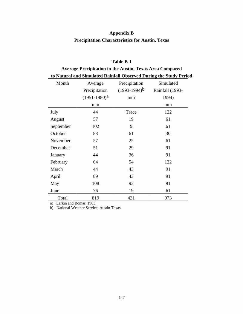
147
Appendix B
Precipitation Characteristics for Austin, Texas
Table B-1
Average Precipitation in the Austin, Texas Area Compared
to Natural and Simulated Rainfall Observed During the Study Period
Month Average
Precipitation
(1951-1980)a
mm
Precipitation
(1993-1994)b
mm
Simulated
Rainfall (1993-
1994)
mm
July 44 Trace 122
August 57 19 61
September 102 9 61
October 83 61 30
November 57 25 61
December 51 29 91
January 44 36 91
February 64 54 122
March 44 43 91
April 89 43 91
May 108 93 91
June 76 19 61
Total 819 431 973a) Larkin and Bomar, 1983b) National Weather Service, Austin Texas

148
Table B-2
Rainfall Frequency for Austin, Texas (rainfall given in mm)Duration(hrs)--------Freq.(yrs)
1/12-----
1/4-----
1/2-----
1-----
2------
3------
6------
12------
24------
1 33 41 48 53 61 71 81
2 13 28 41 51 58 66 79 89 104
5 51 64 79 86 104 122 140
10 58 74 91 102 122 145 170
25 69 86 109 119 147 173 201
50 79 99 122 135 163 196 226
100 22 48 86 107 135 152 183 221 254

149
Appendix C
Water Droplet Trajectory
The amount of energy required to throw a water droplet a given distance is
illustrated by comparing the throw distance of a droplet to that of a stream with the same
nozzle exit velocity. It is a common simplification to model water streams as a
continuous, frictionless stream traveling through the air. The trajectory of the water
stream is that of a parabola if air drag is neglected. Figure C.1 depicts the trajectory of a
water stream leaving a 4.8-mm-diameter straight nozzle under 276 millipascal pressure.
The flow rate is 0.4 L/sec and the exit velocity (Ve) is 23 m/sec. The nozzle is mounted at
an elevation of 4.3 m and has a 300 departure angle. The height (z) of travel of the stream
can be calculated as:
zV
gm
mmz
o
= = =2 2
22
30 23
2 9 86 7
[(sin )( / sec)]
( . / sec ). (Eq. C.1)
The time (T) to reach this height is found using the equation:
z m V T gT m T m Tz= = + = +6 7 05 30 23 0 5 9 82 0 2 2. . sin ( / sec) . ( . / sec ) (Eq. C.2)
When solving Equation C.2 using the quadratic equation, T is found to be 0.48 seconds.
Using this value of T, the horizontal distance traveled is determined as:
x V T m mx= = =cos ( / sec)( . sec) .30 23 0 48 9 60(Eq. C.3)
The ultimate distance of travel of the water stream can now be found using an approach
similar to the above or by defining the equation for the parabola as shown in Figure C.1.
The flight of water droplets is extremely difficult to model. Evaporation, drag
forces, and lift forces all affect the trajectory of the droplet. The following analysis
makes use of Newton's second law to illustrate the effect of air drag on the travel of a
water droplet from an elevated spray stand. The same initial velocity (23 m/sec) is used
as in the water stream example. However, to simplify the calculation, the assumption is
made that the trajectory is relatively flat and the water droplet leaves the spray head at a
zero degree angle (i.e., flat) with respect to the x-axis. The coefficient of drag (Cd) is
considered to be 0.03, and if there is little spin of the drop, the coefficient of lift can be

150
considered zero. Assuming no loss of mass (i.e., evaporation) from the droplet during
flight, the following equation can be developed for time of flight (sec) to a particular
distance:
tC Sx
mD= −
1
21
βρ
[exp( )] (Eq. C.5)
where:
β =ρC SV
mD x
2 (sec)
Vx = Velocity (m/sec)
r = density of air (mg/l)
m = mass of droplet (g)
S = effective area of droplet (m2)
x = distance along x axis of flight (m)
The y-coordinate, which represents the drop in flight of the droplet, is determined by:
ygt m t
t=−
=−
= −2 2 2
2
2
23
2115
( / sec ). (m) (Eq. C.7)
Figure C.2 shows the flight paths of 4 different droplet sizes from a 4.3-meter
elevated spray head as calculated from the above equations. Comparing Figures C.1 and
C.2 illustrates the additional energy required to produce rainfall versus a water stream.
The throw distances shown in Figure C.2 are very close to those observed during
experiments with the rainfall simulator.

151
Parabolic Trajectory of Water Stream
0.0
2.0
4.0
6.0
8.0
10.0
12.0
0.0 5.0 10.0 15.0 20.0 25.0
Throw Distance (m)
Hei
gh
t o
f S
trea
m (
m)
Figure C.1 Trajectory of Water Stream from a nozzle elevationof 4.3m (nozzle angle = 300)
Throw Distance vs. Droplet Diameter
0
0.5
1
1.5
2
2.5
3
3.5
4
4.5
0 2 4 6 8 10 12 14 16
Throw Distance (m)
Ele
vati
on
(m
)
0.8
1.2
1.6
2.3
Droplet Dia.(mm)
Water Droplet Trajectory
Figure C.2 Water Droplet Trajectory (nozzle angle = 00)

152

153
Appendix DProbability Plots
TSS Normal Probability Plot
-200
0
200
400
600
800
1000
-3 -2 -1 0 1 2 3
Z Score
EM
C (
mg
/l)
(a)
TSS Log Probability Plot
0
1
2
3
4
5
6
7
8
-3 -2 -1 0 1 2 3
Z Score
Ln
(EM
C)
(b)
Figure D-1

154
VSS Normal Probability Plot
-20
0
20
40
60
80
100
120
140
-3 -2 -1 0 1 2 3
Z Score
EM
C (
mg
/l)
(a)
VSS Log Probability Plot
0
0.5
11.5
2
2.5
3
3.54
4.5
5
-3 -2 -1 0 1 2 3
Z Score
Ln
(E
MC
)
(b)
Figure D-2

155
BOD5 Normal Probability Plot
-20
-10
0
10
20
30
40
50
60
-3 -2 -1 0 1 2 3
Z Score
EM
C (
mg
/l)
(a)
BOD5 Log Probability Plot
-2
-1
0
1
2
3
4
5
-3 -2 -1 0 1 2 3
Z Score
Ln
(E
MC
)
(b)
Figure D-3

156
COD Normal Probability Plot
-100
0
100
200
300
400
500
-3 -2 -1 0 1 2 3
Z Score
EM
C (
mg
/l)
(a)
COD Log Probability Plot
0
1
2
3
4
5
6
7
-3 -2 -1 0 1 2 3
Z Score
Ln
(E
MC
)
(b)
Figure D-4

157
Total Carbon Normal Probability Plot
-20
0
20
40
60
80
100
120
140
160
-3 -2 -1 0 1 2 3
Z Score
EM
C (
mg
/l)
(a)
Total Carbon Log Probability Plot
0
1
2
3
4
5
6
-3 -2 -1 0 1 2 3
Z Score
Ln
(E
MC
)
(b)
Figure D-5

158
Dissolved Total Carbon Normal Probability Plot
-40
-20
0
20
40
60
80
100
-3 -2 -1 0 1 2 3
Z Score
EM
C (
mg
/l)
(a)
Dissolved Total Carbon Log Probability Plot
0
0.5
1
1.5
2
2.5
3
3.5
4
4.5
5
-3 -2 -1 0 1 2 3
Z Score
Ln
(E
MC
)
(b)
Figure D-6

159
Nitrate Normal Probability Plot
-1.00
-0.50
0.00
0.50
1.00
1.502.00
2.50
3.00
3.50
4.00
-3 -2 -1 0 1 2 3
Z Score
EM
C (
mg
/l)
(a)
Nitrate Log Probability Plot
-1.5
-1
-0.5
0
0.5
1
1.5
-3 -2 -1 0 1 2 3
Z Score
Ln
(E
MC
)
(b)
Figure D-7

160
Total Phosphorus Normal Probability Plot
-0.40
-0.20
0.00
0.20
0.40
0.60
0.80
1.00
1.20
-3 -2 -1 0 1 2 3
Z Score
EM
C (
mg
/l)
(a)
Total Phosphorus Log Probability Plot
-3.5
-3
-2.5
-2
-1.5
-1
-0.5
0
0.5
-3 -2 -1 0 1 2 3
Z Score
Ln
(E
MC
)
(b)
Figure D-8

161
Oil & Grease Normal Probability Plot
-10
-5
05
10
15
20
2530
35
40
-3 -2 -1 0 1 2 3
Z Score
EM
C (
mg
/l)
(a)
Oil & Grease Log Probability Plot
-0.5
0
0.5
1
1.5
2
2.5
3
3.5
4
-3 -2 -1 0 1 2 3
Z Score
Ln
(E
MC
)
(b)
Figure D-9

162
Copper Normal Probability Plot
-0.040
-0.020
0.000
0.020
0.040
0.060
0.080
0.100
0.120
0.140
-3 -2 -1 0 1 2 3
Z Score
EM
C (
mg
/l)
(a)
Copper Log Probability Plot
-9
-8
-7
-6
-5
-4
-3
-2
-1
0
-3 -2 -1 0 1 2 3
Z Score
Ln
(E
MC
)
(b)
Figure D-10

163
Iron Normal Probability Plot
-2.0
0.0
2.0
4.0
6.0
8.0
10.0
12.0
-3 -2 -1 0 1 2 3
Z Score
EM
C (
mg
/l)
(a)
Iron Log Probability Plot
-1.5
-1
-0.5
0
0.5
1
1.5
2
2.5
3
-3 -2 -1 0 1 2 3
Z Score
Ln
(E
MC
)
(b)
Figure D-11

164
Lead Normal Probability Plot
-0.10
0.00
0.10
0.20
0.30
0.40
0.50
-3 -2 -1 0 1 2 3
Z Score
EM
C (
mg
/l)
(a)
Lead Log Probability Plot
-6
-5
-4
-3
-2
-1
0
-3 -2 -1 0 1 2 3
Z Score
Ln
(E
MC
)
(b)
Figure D-12

165
Zinc Normal Probability Plot
-0.20-0.100.000.100.200.300.400.500.600.700.800.90
-3 -2 -1 0 1 2 3
Z Score
EM
C (
mg
/l)
(a)
Zinc Log Probability Plot
-12
-10
-8
-6
-4
-2
0
2
-3 -2 -1 0 1 2 3
Z Score
Ln
(E
MC
)
(b)
Figure D-13

166

167
Appendix EHistograms of Constituent Event Mean Concentrations
0
2
4
6
8
10
12
0 100 200 300 400 500 600 700 800 900
Series: TSSSample 1 60Observations 56
Mean 280.8329Median 263.9532Maximum 913.5640Minimum 32.84788Std. Dev. 176.3990Skewness 1.331434Kurtosis 5.369535
Jarque-Bera 29.64630Probability 0.000000
Figure E-1 Histogram of TSS Observations
0
2
4
6
8
10
12
10 20 30 40 50 60 70 80 90 100 110 120 130
Series: VSSSample 1 60Observations 56
Mean 40.25125Median 37.75149Maximum 129.6032Minimum 8.043515Std. Dev. 22.32028Skewness 1.909382Kurtosis 7.693938
Jarque-Bera 85.43738Probability 0.000000
Figure E-2 Histogram of VSS Observations

168
0
4
8
12
16
0 10 20 30 40 50
Series: BOD5Sample 1 60Observations 56
Mean 10.26243Median 5.635188Maximum 55.96183Minimum 0.000000Std. Dev. 11.90662Skewness 1.818289Kurtosis 6.207110
Jarque-Bera 54.85727Probability 0.000000
Figure E-3 Histogram of BOD5 Observations
0
4
8
12
16
0 50 100 150 200 250 300 350 400 450
Series: CODSample 1 60Observations 59
Mean 115.2954Median 85.68171Maximum 451.8942Minimum 23.65436Std. Dev. 81.07346Skewness 1.876978Kurtosis 7.069881
Jarque-Bera 75.36296Probability 0.000000
Figure E-4 Histogram of COD Observations

169
0
4
8
12
16
20 40 60 80 100 120 140 160
Series: TOTAL_CARBONSample 1 60Observations 58
Mean 55.98013Median 47.40649Maximum 153.1323Minimum 15.52180Std. Dev. 31.75266Skewness 1.381747Kurtosis 4.381232
Jarque-Bera 23.06636Probability 0.000010
Figure E-5 Histogram of Total Carbon Observations
0
4
8
12
16
0 10 20 30 40 50 60 70 80 90
Series: DISSOLVED_TCSample 1 60Observations 58
Mean 23.85538Median 16.28556Maximum 89.15573Minimum 1.508748Std. Dev. 21.53276Skewness 1.740246Kurtosis 5.072970
Jarque-Bera 39.65998Probability 0.000000
Figure E-6 Histogram of Dissolved Total Carbon Observations

170
0
5
10
15
20
0.5 1.0 1.5 2.0 2.5 3.0 3.5
Series: NITRATESample 4 60Observations 52
Mean 1.072430Median 0.834079Maximum 3.655834Minimum 0.360000Std. Dev. 0.752601Skewness 2.120103Kurtosis 6.865016
Jarque-Bera 71.32168Probability 0.000000
Figure E-7 Histogram of Nitrate Observations
0
2
4
6
8
10
12
0.0 0.2 0.4 0.6 0.8 1.0
Series: PHOSPHORUSSample 1 60Observations 57
Mean 0.364631Median 0.301269Maximum 1.094537Minimum 0.043548Std. Dev. 0.246396Skewness 1.292763Kurtosis 4.049037
Jarque-Bera 18.49037Probability 0.000097
Figure E-8 Histogram of Total Phosphorus Observations

171
0
5
10
15
20
25
30
0 5 10 15 20 25 30 35
Series: OIL_GREASESample 1 58Observations 35
Mean 5.329703Median 4.000000Maximum 35.11179Minimum 0.832557Std. Dev. 6.369516Skewness 3.709168Kurtosis 16.23923
Jarque-Bera 335.8670Probability 0.000000
Figure E-9 Histogram of Oil and Grease Observations
0
2
4
6
8
10
0.00 0.02 0.04 0.06 0.08 0.10 0.12
Series: COPPERSample 1 60Observations 55
Mean 0.029204Median 0.020003Maximum 0.121927Minimum 0.000000Std. Dev. 0.025704Skewness 1.272323Kurtosis 4.500350
Jarque-Bera 19.99772Probability 0.000045
Figure E-10 Histogram of Copper Observations

172
0
2
4
6
8
0 2 4 6 8 10
Series: IRONSample 1 60Observations 56
Mean 3.928788Median 3.480462Maximum 10.11041Minimum 0.000000Std. Dev. 2.370751Skewness 0.755700Kurtosis 3.314401
Jarque-Bera 5.560755Probability 0.062015
Figure E-11 Histogram of Iron Observation
0
2
4
6
8
10
0.0 0.1 0.2 0.3 0.4
Series: LEADSample 9 60Observations 47
Mean 0.108971Median 0.081356Maximum 0.435537Minimum 0.000000Std. Dev. 0.093328Skewness 1.364516Kurtosis 4.925249
Jarque-Bera 21.84363Probability 0.000018
Figure E-12 Histogram of Lead Observations

173
0
2
4
6
8
10
12
0.0 0.1 0.2 0.3 0.4 0.5 0.6 0.7 0.8
Series: ZINCSample 1 60Observations 56
Mean 0.217646Median 0.178833Maximum 0.814556Minimum 0.000000Std. Dev. 0.173119Skewness 1.303050Kurtosis 4.684838
Jarque-Bera 22.47102Probability 0.000013
Figure E-13 Histogram of Zinc Observations

175
Appendix F
Constituent Wash-Off Patterns
TSS
0
200
400
600
800
1000
0 20000 40000 60000 80000Cumulative Flow (liters)
Co
nce
ntr
atio
n (
mg
/l)
Traffic No-Traff ic
(a) Median TSS Concentration During a Simulated Storm Event
TSS
0
1
2
3
4
5
0 20000 40000 60000 80000Cumulative Flow (liters)
Lo
ad (
g/m
)
Traffic No-Traff ic
(b) Median TSS Load During a Simulated Storm Event
TSS
0
2
4
6
8
10
12
0 20000 40000 60000 80000 100000Cumulative Flow (liters)
Lo
ad (
g/m
)
Simulated Natural
(c) TSS Load During Natural and Simulated Storm Events
Figure F-1

176
VSS
0
20
40
60
80
100
0 20000 40000 60000 80000Cumulative Flow (liters)
Co
nce
ntr
atio
n (
mg
/l)
Traffic No-Traff ic
(a) Median VSS Concentration During a Simulated Storm Event
VSS
0
0.1
0.2
0.3
0.4
0.5
0.6
0 20000 40000 60000 80000Cumulative Flow (liters)
Lo
ad (
g/m
)
Traffic No-Traff ic
(b) Median VSS Load During a Simulated Storm Event
VSS
0
0.2
0.4
0.6
0.8
1
1.2
0 20000 40000 60000 80000 100000Cumulative Flow (liters)
Lo
ad (
g/m
)
Simulated Natural
(c) VSS Load During Natural and Simulated Storm Events
Figure F-2

177
BOD
0
5
10
15
20
25
30
0 20000 40000 60000 80000Cumulative Flow (liters)
Co
nce
ntr
atio
n (
mg
/l)
Traffic No-Traff ic
(a) Median BOD5 Concentration During a Simulated Storm Event
BOD
0
0.01
0.02
0.03
0.04
0.05
0 20000 40000 60000 80000Cumulative Flow (liters)
Lo
ad (
g/m
)
Traffic No-Traff ic
(b) Median BOD5 Load During a Simulated Storm Event
BOD
0
0.05
0.1
0.15
0.2
0.25
0 20000 40000 60000 80000 100000Cumulative Flow (liters)
Lo
ad (
g/m
)
Simulated Natural
(c) BOD5 Load During Natural and Simulated Storm Events
Figure F-3

178
COD
0
50
100
150
200
250
0 20000 40000 60000 80000Cumulative Flow (liters)
Co
nce
ntr
atio
n (
mg
/l)
Traffic No-Traff ic
(a) Median COD Concentration During a Simulated Storm Event
COD
0
0.2
0.4
0.6
0.8
1
1.2
0 20000 40000 60000 80000Cumulative Flow (liters)
Lo
ad (
g/m
)
Traffic No-Traff ic
(b) Median COD Load During a Simulated Storm Event
COD
0
0.5
1
1.5
2
2.5
0 20000 40000 60000 80000 100000Cumulative Flow (liters)
Lo
ad (
g/m
)
Simulated Natural
(c) COD Load During Natural and Simulated Storm Events
Figure F-4

179
Total Carbon
0
20
40
60
80
100
120
140
0 20000 40000 60000 80000Cumulative Flow (liters)
Co
nce
ntr
atio
n (
mg
/l)
Traffic No-Traff ic
(a) Median Total Carbon Concentration During a Simulated Storm Event
Total Carbon
0
0.1
0.2
0.3
0.4
0.5
0.6
0.7
0 20000 40000 60000 80000Cumulative Flow (liters)
Lo
ad (
g/m
)
Traffic No-Traff ic
(b) Median Total Carbon Load During a Simulated Storm Event
Total Carbon
00.20.40.60.8
11.21.41.6
0 20000 40000 60000 80000 100000Cumulative Flow (liters)
Lo
ad (
g/m
)
Simulated Natural
(c) Total Carbon Load During Natural and Simulated Storm Events
Figure F-5

180
Dissolved Total Carbon
0
10
20
30
40
50
0 20000 40000 60000 80000Cumulative Flow (liters)
Co
nce
ntr
atio
n (
mg
/l)
Traffic No-Traff ic
(a) Median Dissolved TC Concentration During a Simulated Storm Event
Dissolved Total Carbon
0
0.05
0.1
0.15
0.2
0 20000 40000 60000 80000Cumulative Flow (liters)
Lo
ad (
g/m
)
Traffic No-Traff ic
(b) Median Dissolved TC Load During a Simulated Storm Event
Dissolved Total Carbon
0
0.1
0.2
0.3
0.4
0.5
0 20000 40000 60000 80000 100000Cumulative Flow (liters)
Lo
ad (
g/m
)
Simulated Natural
(c) Dissolved TC Load During Natural and Simulated Storm Events
Figure F-6

181
Nitrate
0
0.2
0.4
0.6
0.8
1
1.2
0 20000 40000 60000 80000Cumulative Flow (liters)
Co
nce
ntr
atio
n (
mg
/l)
Traffic No-Traff ic
(a) Median Nitrate Concentration During a Simulated Storm Event
Nitrate
0
0.002
0.004
0.006
0.008
0.01
0.012
0.014
0 20000 40000 60000 80000Cumulative Flow (liters)
Lo
ad (
g/m
)
Traffic No-Traff ic
(b) Median Nitrate Load During a Simulated Storm Event
Nitrate
0
0.005
0.01
0.015
0.02
0.025
0 20000 40000 60000 80000 100000Cumulative Flow (liters)
Lo
ad (
g/m
)
Simulated Natural
(c) Nitrate Load During Natural and Simulated Storm Events
Figure F-7

182
TP
0
0.1
0.2
0.3
0.4
0.5
0.6
0.7
0 20000 40000 60000 80000Cumulative Flow (liters)
Co
nce
ntr
atio
n (
mg
/l)
Traffic No-Traff ic
(a) Median Phosphorus Concentration During a Simulated Storm Event
TP
0
0.0005
0.001
0.0015
0.002
0.0025
0.003
0.0035
0 20000 40000 60000 80000Cumulative Flow (liters)
Lo
ad (
g/m
)
Traffic No-Traff ic
(b) Median Phosphorus Load During a Simulated Storm Event
TP
00.0010.0020.0030.0040.0050.0060.0070.008
0 20000 40000 60000 80000 100000Cumulative Flow (liters)
Lo
ad (
g/m
)
Simulated Natural
(c) Phosphorus Load During Natural and Simulated Storm Events
Figure F-8

183
O&G
00.5
1
1.52
2.53
3.54
0 20000 40000 60000 80000Cumulative Flow (liters)
Co
nce
ntr
atio
n (
mg
/l)
Traffic No-Traff ic
(a) Median Oil and Grease Concentration During a Simulated Storm Event
O&G
0
0.01
0.02
0.03
0.04
0.05
0.06
0 20000 40000 60000 80000Cumulative Flow (liters)
Lo
ad (
g/m
)
Traffic No-Traff ic
(b) Median Oil and Grease Load During a Simulated Storm Event
O&G
0
0.02
0.04
0.06
0.08
0.1
0 20000 40000 60000 80000 100000Cumulative Flow (liters)
Lo
ad (
g/m
)
Simulated Natural
(c) Oil and Grease Load During Natural and Simulated Storm Events
Figure F-9

184
Copper
0
0.01
0.02
0.03
0.04
0.05
0.06
0 20000 40000 60000 80000Cumulative Flow (liters)
Co
nce
ntr
atio
n (
mg
/l)
Traffic No-Traff ic
(a) Median Copper Concentration During a Simulated Storm Event
Copper
0
0.00005
0.0001
0.00015
0.0002
0.00025
0.0003
0 20000 40000 60000 80000Cumulative Flow (liters)
Lo
ad (
g/m
)
Traffic No-Traff ic
(b) Median Copper Load During a Simulated Storm Event
Copper
0
0.0002
0.0004
0.0006
0.0008
0.001
0 20000 40000 60000 80000 100000Cumulative Flow (liters)
Lo
ad (
g/m
)
Simulated Natural
(c) Copper Load During Natural and Simulated Storm Events
Figure F-10

185
Iron
012
3456
78
0 20000 40000 60000 80000Cumulative Flow (liters)
Co
nce
ntr
atio
n (
mg
/l)
Traffic No-Traff ic
(a) Median Iron Concentration During a Simulated Storm Event
Iron
0
0.01
0.02
0.03
0.04
0.05
0.06
0.07
0 20000 40000 60000 80000Cumulative Flow (liters)
Lo
ad (
g/m
)
Traffic No-Traff ic
(b) Median Iron Load During a Simulated Storm Event
Iron
0
0.02
0.04
0.06
0.08
0.1
0.12
0 20000 40000 60000 80000 100000Cumulative Flow (liters)
Lo
ad (
g/m
)
Simulated Natural
(c) Iron Load During Natural and Simulated Storm Events
Figure F-11

186
Lead
0
0.05
0.1
0.15
0.2
0 20000 40000 60000 80000Cumulative Flow (liters)
Co
nce
ntr
atio
n (
mg
/l)
Traffic No-Traff ic
(a) Median Lead Concentration During a Simulated Storm Event
Lead
0
0.0002
0.0004
0.0006
0.0008
0.001
0.0012
0 20000 40000 60000 80000Cumulative Flow (liters)
Lo
ad (
g/m
)
Traffic No-Traff ic
(b) Median Lead Load During a Simulated Storm Event
Lead
0
0.0005
0.001
0.0015
0.002
0.0025
0.003
0 20000 40000 60000 80000 100000Cumulative Flow (liters)
Lo
ad (
g/m
)
Simulated Natural
(c) Lead Load During Natural and Simulated Storm Events
Figure F-12

187
Zinc
00.10.2
0.30.40.50.6
0.70.8
0 20000 40000 60000 80000Cumulative Flow (liters)
Co
nce
ntr
atio
n (
mg
/l)
Traffic No-Traff ic
(a) Median Zinc Concentration During a Simulated Storm Event
Zinc
0
0.0005
0.001
0.0015
0.002
0.0025
0 20000 40000 60000 80000Cumulative Flow (liters)
Lo
ad (
g/m
)
Traffic No-Traff ic
(b) Median Zinc Load During a Simulated Storm Event
Zinc
00.0010.0020.0030.0040.0050.0060.0070.008
0 20000 40000 60000 80000 100000Cumulative Flow (liters)
Lo
ad (
g/m
)
Simulated Natural
(c) Zinc Load During Natural and Simulated Storm Events
Figure F-13

188

189
Appendix G
The Method of Generalized Least Squares:
Corrections for Heteroscedasticity and Autocorrelation
Introduction
Least squares regression is a method used to determine the line of average
relationship between a single dependent variable and one or more explanatory, or
independent, variables. Consider the simple relationship between COD load, the
dependent variable, and total volume of storm flow, the independent variable, illustrated
in Figure G-1. Although COD load increases in direct proportion to an increase in total
storm flow, there is substantial variation in the value of COD load for individual values
of storm flow. The best the regression model can do is estimate the expected, or average,
COD load for a given storm size. The regression model assumes that the “disturbances,”
or the variations from the expected value, are “well behaved,” meaning that their
expected value is zero, their variance is constant, and they are not correlated with each
other. The problems that arise when the disturbances are not well behaved are the subject
of this appendix.
Rationale for the Disturbance Term
The regression line illustrated in Figure G-1 is described by the linear function:
COD Flow= +0 548 0 0002. . ( ) (G-1)
Equation G-1 is not mathematically correct because not all (probably not any) of
the values of COD are truly equal to the right-hand side of the equation. To achieve the
identity, G-1 must be reformulated to include a disturbance term e defined as the
difference between the observed value of COD and the equation value of COD for a
specific value of flow.
COD Flow ei i i= + +0 548 0 0002. . ( ) (G-2)

190
Given a set of observations, each disturbance term e is measurable and is referred to as
the “residual.” The values of the residuals can be either positive, negative, or zero and
are collectively described by a normal probability distribution. The variance of this
distribution determines the standard error of regression, which is a measure of the
“goodness of fit” of the regression equation.
Adding a disturbance term to equation G-1 may seem like an arbitrary
mathematical fix, but there are several important reasons for the existence of disturbance
in the data set. First, not all of the relevant variables may have been included in the
regression. In the previous example, only about 69% of the variation in COD is
explained by total storm flow. There also are other variables that act in conjunction with
flow to influence COD loads, such as traffic volume, traffic mix, antecedent dry period,
etc.
0
2
4
6
8
1 0
0 5 0 0 0 1 0 0 0 0 1 5 0 0 0 2 0 0 0 0 2 5 0 0 0 3 0 0 0 0
Storm Flow (gal)
CO
D L
oad
(kg)
Figure G-1
Second, it is possible that the COD load measured during the storm was measured
in error. This error could result from any number of reasons, including mishandling of
the sample, mishap in the laboratory analysis, or a simple recording error, just to name a
few.

191
Third, the disturbance could be the result of an inherently random component in
the system under study. Natural systems are notoriously difficult to predict, and there
could be any number of explanatory variables that have inherently random components.
Method of Ordinary Least Squares
The method of ordinary least squares (OLS) is the usual way to calculate the
coefficients of a regression equation. OLS provides a simple procedure for calculating
the coefficients of an inexact linear function by minimizing the sum of the squared
differences, e2 , between the observed values of the dependent variable Y and the
estimated values $Y . Furthermore, the OLS coefficients computed from a sample are the
minimum-variance, linear, unbiased estimators of the population regression coefficients
only if certain assumptions are satisfied. Mathematically, the OLS procedure is defined
as
minimize e Y Yi i i2 2= −∑∑ ( $ ) (G-3)
where expression G-3 is often referred to as the error sum of squares (ESS) or the
residual sum of squares.
Although OLS guarantees the “best” linear fit of the sample data, it is not
necessarily the “best linear and unbiased estimator” (BLUE) for the population regression
coefficients. Unlike the sample disturbance term e, the population disturbance term,
denoted as U, is not observable. Consequently, the following assumptions must be made
regarding the statistical properties of the population disturbance term U to complete the
specification of the OLS model:
1. The disturbance term is normally distributed, and therefore the expected value, or
mean, of all U's for any given value of Y is zero.
2. All values of U, associated with different values of an independent variable X,
have the same variance (homoscedastic assumption).
3. Each value of U is independent of all other values of U (uncorrelated residuals).
4. The value of any independent variable X is independent of the value of U.

192
The complete OLS model specifies both the population regression equation and
the parameters of the distribution of the population disturbance term. The population
regression equation derived from the data in Figure G-1 contains two distinct statements:
a scientific statement [ 0 548 0 0002. . ( )+ Flowi ] and a statistical statement (U and its
distribution).
If any of the assumptions regarding the distributional properties of the disturbance
terms are violated, the OLS coefficients will not be BLUE. Unfortunately, the highway
runoff data collected during the course of this research exhibit the characteristics of both
heteroscedasticity and autocorrelation, which are two of the most common violations of
the disturbance term assumptions. The procedures used to identify misspecified
disturbance terms, the consequences of applying OLS procedures in the presence of a
misspecified disturbance term, and the remedies used to correct for such
misspecifications, are discussed in the remainder of this appendix.
Heteroscedasticity
Heteroscedasticity is the formal name that describes the condition in that the
variance of the residuals is not uniform across the range of an explanatory variable X.
This condition is common in cross-sectional data where the observations of variables of
differing magnitudes are collected at a single point in time. Re-consider the data plotted
in Figure G-1. It is apparent that the variance for the COD load increases as the storm
flow increases. One possible explanation for this phenomenon is that the COD loads may
vary with storm intensity. For example, low-intensity storms might produce smaller
COD loads than higher intensity storms, regardless of the duration, and consequently the
storm volume. In any case, the values for COD load are not as variable for low storm
flows as they are for the higher volume flows. This is a classic illustration of
heteroscedasticity in cross-sectional data.
It can be shown that the OLS estimate of the population regression coefficients is
an unbiased estimator regardless of the distributional properties (i.e., the variance or
correlation) of the population disturbance term. However, the OLS coefficients are not
the minimum variance estimators if the homoscedastic assumption of the disturbance

193
term is violated. This is because the most inaccurate observations, or the observations
with the largest variances, will dominate the ESS calculation. In other words, OLS will
minimize an ESS that is heavily influenced by the observations that have the largest
variances. Furthermore, this same calculation will lead to a biased estimate of the
population variance (e.g., on average, the variance will be either underestimated or
overestimated), which in turn will lead to a biased estimate of the variance of the
population regression coefficients. The result is that conventionally computed
confidence intervals and the conventionally employed t and F tests are no longer valid. If
the population variance is underestimated (there is no theoretical basis for determining
the direction of the bias), the computed confidence intervals will be narrower than they
should be, providing an ill-founded belief in the precision of the model. A complete
mathematical justification regarding the effects of misspecified disturbance terms is
found in Johnson et. al., 1987.
Method of Generalized Least Squares
The ideal regression estimating scheme should give less importance, or “weight,”
to those observations coming from populations with greater variability than those that
come from populations of smaller variability. Unfortunately, OLS does not follow this
strategy, as it assigns equal weight to each observation. But a method known as
generalized least squares (GLS) does follow this strategy and is capable of producing
estimators that are BLUE. To illustrate GLS, re-consider the COD-storm flow model:
COD Flow Ui i i= + +0 548 0 0002. . ( ) (G-4)
Assume that the heteroscedastic variances σi2 are known (i.e., E U i i( )2 2= σ ). If equation
G-4 is divided through by σi to obtain:
COD Flow Ui
i i
i
i
i
iσ σ σ σ=
+
+
0548
10 0002. . (G-5)

194
The purpose of this transformation is found in the following feature of the transformed
disturbance term:
varU
EUi
i
i
iσ σ
=
2
since is knowni2=
12
2
σσ
iiE U( )
= since 1
22 2 2
σσ σ
ii i iE U( ) ( ) =
=1, which is a constant (G-6)
The variance of the transformed disturbance term U is now constant, or
homoscedastic. But also note that the effect of this transformation is to weight each
variable by a value that is inversely proportional to its standard deviation, σi. If OLS is
applied to the transformed variables, the COD observations from populations with large
σi will be given proportionately less weight than the COD observations from populations
with smaller σi during the minimizing of the ESS. Since all other OLS assumptions are
retained, the OLS coefficients calculated from the transformed data will be BLUE.
To summarize, the method of GLS is merely OLS performed with a set of
transformed variables that satisfy the OLS assumptions. Unfortunately, GLS is difficult
in practice because the heteroscedastic variances σi2, and subsequently the correct
heteroscedastic transformations, are not known. Furthermore, there is no method to
directly determine the best transformation. The procedure is strictly trial and error. A
transformation is made, the equation is re-estimated using OLS procedures with the
transformed variables, and a statistical test is used to determine if the new disturbance
term is homoscedastic.
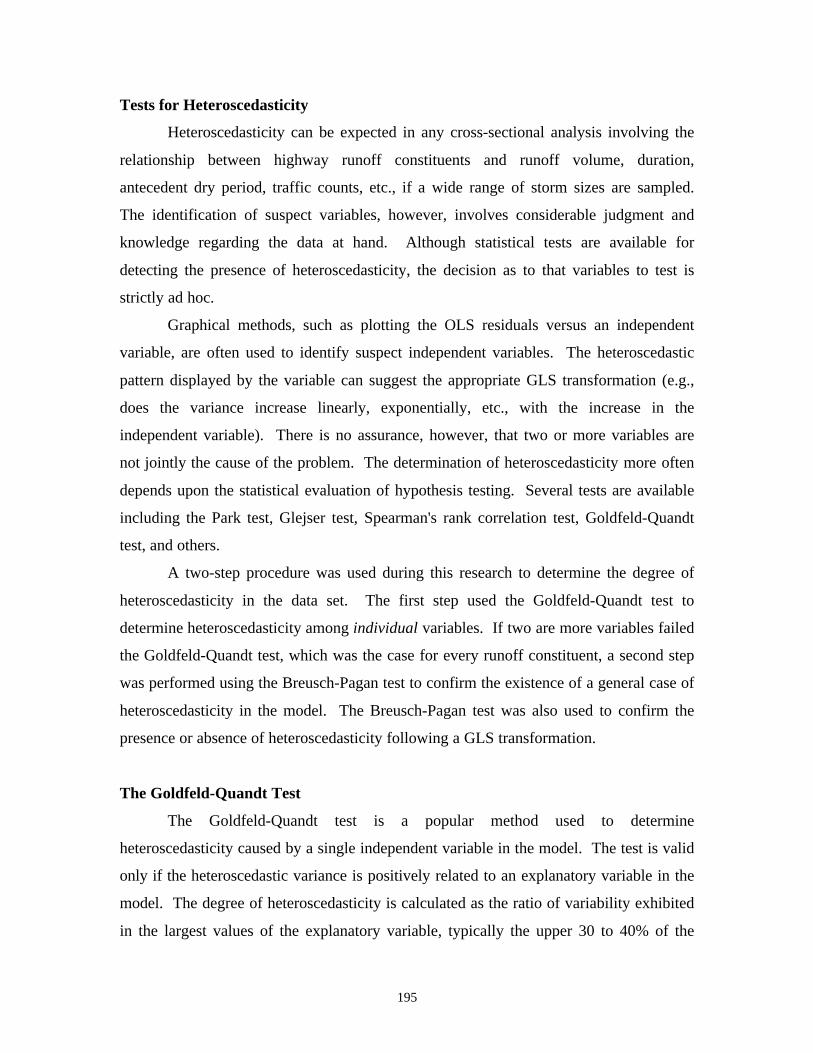
195
Tests for Heteroscedasticity
Heteroscedasticity can be expected in any cross-sectional analysis involving the
relationship between highway runoff constituents and runoff volume, duration,
antecedent dry period, traffic counts, etc., if a wide range of storm sizes are sampled.
The identification of suspect variables, however, involves considerable judgment and
knowledge regarding the data at hand. Although statistical tests are available for
detecting the presence of heteroscedasticity, the decision as to that variables to test is
strictly ad hoc.
Graphical methods, such as plotting the OLS residuals versus an independent
variable, are often used to identify suspect independent variables. The heteroscedastic
pattern displayed by the variable can suggest the appropriate GLS transformation (e.g.,
does the variance increase linearly, exponentially, etc., with the increase in the
independent variable). There is no assurance, however, that two or more variables are
not jointly the cause of the problem. The determination of heteroscedasticity more often
depends upon the statistical evaluation of hypothesis testing. Several tests are available
including the Park test, Glejser test, Spearman's rank correlation test, Goldfeld-Quandt
test, and others.
A two-step procedure was used during this research to determine the degree of
heteroscedasticity in the data set. The first step used the Goldfeld-Quandt test to
determine heteroscedasticity among individual variables. If two are more variables failed
the Goldfeld-Quandt test, which was the case for every runoff constituent, a second step
was performed using the Breusch-Pagan test to confirm the existence of a general case of
heteroscedasticity in the model. The Breusch-Pagan test was also used to confirm the
presence or absence of heteroscedasticity following a GLS transformation.
The Goldfeld-Quandt Test
The Goldfeld-Quandt test is a popular method used to determine
heteroscedasticity caused by a single independent variable in the model. The test is valid
only if the heteroscedastic variance is positively related to an explanatory variable in the
model. The degree of heteroscedasticity is calculated as the ratio of variability exhibited
in the largest values of the explanatory variable, typically the upper 30 to 40% of the

196
range of X, to the variability exhibited in the smallest values of the explanatory variable,
the lowest 30 to 40% of the range of X. If the disturbance terms are assumed to be
normally distributed and if the assumption of homoscedasticity is valid, it can be shown
that this ratio follows the F distribution with numerator and denominator degrees of
freedom equal to ( ) /n d K− − 2 2 , where n is the sample size, d is the number of
observations deleted to calculate the ratio, and K is the number of regression coefficients
estimated (including the intercept). As a hypothesis test, if the computed F-ratio is
greater than the critical F-ratio at the chosen level of significance, the null hypothesis of
homoscedasticity is rejected.
Specifically, the Goldfeld-Quandt test was performed on each explanatory
variable as follows:
1) All observations (423) are sorted by increasing value of the suspect variable.
2) The middle portion of the observations are deleted. In this study, 131
observations were deleted, leaving 146 “low” values and 146 “high” values.
3) The OLS equation is estimated for each of the two subgroups.
4) The computed test statistic is calculated by dividing the error sum of squares
(ESS) of the high group by the ESS of the low group.
5) The computed test statistic is compared to the critical F-statistic. The critical
F-statistic for 139 degrees of freedom (n = 423, d = 131, and K = 7) in the
numerator and 139 degrees of freedom in the denominator at the 0.05 level is
approximately 1.3. If the computed F-statistic is greater than the critical
F-statistic, the null hypothesis of no heteroscedasticity is rejected.
In summary, if the ESS of the upper range is 1.3 times the ESS of the lower range,
the variance across the range of X is considered heteroscedastic.
The structure of the Goldfeld-Quandt test limits the test to identifying
heteroscedasticity caused by a single variable. If the model contains more than one
independent variable, the test should be applied to as many of the variables as possible.
If two or more independent variables are identified as heteroscedastic, it must be assumed
that they jointly contribute heteroscedasticity to the model. In this case, a more general
test should be used to confirm the presence of heteroscedasticity in the model.

197
Table G-1 summarizes the results of the Goldfeld-Quandt test. The results
indicate that storm duration, storm flow, storm vehicle count, and antecedent traffic count
are all suspected of causing heteroscedasticity in each short model. The previous storm
flow is an additional suspect only in the COD short model.
Table G-1 Calculated Test Statistic in Goldfeld-Quandt Test
Constituent Duration Flow Vehicle
Count
Antecedent
Traffic
Previous
Traffic
Previous
Flow
COD 3.1 9.3 3.6 3.2 0.8 1.6
Nitrate 4.5 8.0 4.5 4.0 1.0 0.7
Oil and Grease 12.5 8.3 26.0 3.3 0.4 1.0
TSS 3.0 17.0 5.1 1.9 0.8 0.5
Phosphorous 4.0 9.1 4.0 3.0 0.5 0.9
Copper 9.0 32.9 20.5 3.0 0.1 0.3
Iron 2.5 13.8 4.3 2.9 0.4 0.2
Lead 2.3 22.9 4.8 5.7 0.4 0.1
Zinc 10.0 43.5 22.0 55.0 0.04 0.5
(Critical value of F = 1.3)
The Breusch-Pagan Test
The Breusch-Pagan test is a more general test that examines a model for
heteroscedasticity caused by one or more independent variables. Like the Goldfeld-
Quandt test, a set of suspect variables must be identified prior to application of the test.
In this research, each independent variable that failed the Goldfeld-Quandt test is
assumed to jointly contribute to heteroscedasticity in the model.
The Breusch-Pagan test standardizes each OLS residual by dividing by the
variance of the residuals. This set of standardized residuals is then regressed against the
suspect explanatory variables. A test statistic is calculated as one half of the total sum of
squares minus the ESS. The total sum of squares (SS) is defined as the sum of the
squared deviations of the sample values of the dependent variable about the sample mean
of the dependent variable. This test statistic is distributed as chi-squared with k degrees
of freedom, where k is the number of suspect explanatory variables. Because the

198
condition of homoscedasticity is assumed, the null hypothesis of homoscedasticity is
rejected if the test statistic is larger than the critical value of the chi-square statistic.
Specifically, the Breusch-Pagan test was conducted during this research as
follows:
1) Compute the OLS residuals ( ei
Yi
Yi
= − $ ) for the model, where Y is the
observed value of the dependent variable and $Y is the regression value.
2) Calculate e Si e2 2/ , where S e ne i
2 2= ∑ / and n = number of observations.
3) Regress the standardized OLS residuals, e Si i2 2/ , on the suspect independent
variables.
4) Calculate the test statistic as (SS - ESS) / 2 where SS is the Total Sum of
Squares RESSSS
2 1= −
5) If the test statistic is greater than the critical value of the chi-square statistic,
the null hypothesis of homoscedasticity is rejected. The critical value of chi-
square distribution at the 0.05 level with 4 degrees of freedom (e.g., 4 suspect
variables) is 9.49.
Heteroscedasticity Transformations
Consider the structure of the following highway runoff model estimated by OLS:
Y D F V A PV PF Ui i i i i i i i= + + + + + + +β β β β β β β0 1 2 3 4 5 6 (G-7)
where Yi = dependent variable (kg/m2);
βi = regression coefficients;
Di = storm duration (min);
Fi = storm flow (L/m2);
Vi = average # of vehicles per lane during the storm;
Ai = average # of vehicles per lane during the antecedent dry period;

199
PVi = average # of vehicles per lane during the previous storm;
PFi = flow during the previous storm (L/m2)
Ui = disturbance term
As shown in Table G-1, the Goldfeld-Quandt test determined that each of the
explanatory variables, with the exception of PV and PF, contributed heteroscedasticity in
the base model (PF only contributed in the COD data set). Furthermore, the Breusch-
Pagan test also confirmed a general case of heteroscedasticity in the base model.
Therefore, a GLS transformation must be found such that the disturbance term of the
transformed equation is homoscedastic. As noted above, there is no automatic method
for determining the “best” transformation. The process is purely trial and error until an
acceptable transformation is found. The obvious starting point is to assume that the
heteroscedastic variances are directly related to each variable that failed the Goldfeld-
Quandt test. Other possibilities include heteroscedastic variances that are related to the
estimated values of the dependent variable, or related to the OLS residuals themselves.
In all, 13 transformations were performed for the purpose of correcting for
heteroscedasticity. The logic behind each transformation is described below.
Transformation I-a: Assumes that the heteroscedastic variance is a linear function of
storm duration (i.e., E U Di i( )2 2= σ ). The transformed equation to be estimated by OLS
is:
Y
D D
D
D
F
D
V
D
A
D
PV
D
PF
D
U
Di
io
i
i
i
i
i
i
i
i
i
i
i
i
i
i
i
= + + + + + + +β β β β β β β1
1 2 3 4 5 6
Transformation I-b: Assumes that the heteroscedastic variance is a linear function of
storm flow (i.e., E U Fi i( )2 2= σ ). The transformed equation to be estimated by OLS is:
Y
F F
D
F
F
F
V
F
A
F
PV
F
PF
F
U
Fi
io
i
i
i
i
i
i
i
i
i
i
i
i
i
i
i
= + + + + + + +β β β β β β β1
1 2 3 4 5 6

200
Transformation I-c: Assumes that the heteroscedastic variance is a linear function of
vehicle intensity (i.e., E U Vi i( )2 2= σ ). The transformed equation to be estimated by OLS
is:
Y
V V
D
V
F
V
V
V
A
V
PV
V
PF
V
U
Vi
io
i
i
i
i
i
i
i
i
i
i
i
i
i
i
i
= + + + + + + +β β β β β β β1
1 2 3 4 5 6
Transformation Id: Assumes that the heteroscedastic variance is a linear function of
antecedent traffic count changes (i.e., E U Ai i( )2 2= σ ). The transformed equation to be
estimated by OLS is:
Y
A A
D
A
F
A
V
A
A
A
PV
A
PF
A
U
Ai
io
i
i
i
i
i
i
i
i
i
i
i
i
i
i
i
= + + + + + + +β β β β β β β1
1 2 3 4 5 6
Transformation I-e: Assumes that the heteroscedastic variance is a linear function of
the previous storm flow (i.e., E U PFi i( )2 2= σ ). The transformed equation to be
estimated by OLS is:
Y
PF PF
D
PF
F
PF
V
PF
A
PF
PV
PFi
io
i
i
i
i
i
i
i
i
i
i
i
= + + + + +β β β β β β1
1 2 3 4 5
+ +β6
PF
PF
U
PFi
i
i
i
Transformation II-a: Assumes that the heteroscedastic variance changes at an increasing
rate as storm duration changes (i.e., E U Di i( )2 2 2= σ ). The transformed equation to be
estimated by OLS is:
YD D
FD
VD
AD
PVD
PFD
UD
i
io
i
i
i
i
i
i
i
i
i
i
i
i
i
= + + + + + + +β β β β β β β1
1 2 3 4 5 6
Transformation II-b: Assumes that the heteroscedastic variance changes at an increasing
rate as flow changes (i.e., E U Fi i( )2 2 2= σ ). The transformed equation to be estimated by
OLS is:

201
YF F
DF
VF
AF
PVF
PFF
UF
i
io
i
i
i
i
i
i
i
i
i
i
i
i
i
= + + + + + + +β β β β β β β1
1 2 3 4 5 6
Transformation II-c: Assumes that the heteroscedastic variance changes at an increasing
rate as vehicle intensity changes (i.e., E U Vi i( )2 2 2= σ ). The transformed equation to be
estimated by OLS is:
YV V
DV
FV
AV
PVV
PFV
UV
i
io
i
i
i
i
i
i
i
i
i
i
i
i
i
= + + + + + + +β β β β β β β1
1 2 3 4 5 6
Transformation II-d: Assumes that the heteroscedastic variance changes at an increasing
rate as antecedent traffic count (i.e., E U Ai i( )2 2 2= σ ). The transformed equation to be
estimated by OLS is:
YA A
DA
FA
VA
PVA
PFA
UA
i
io
i
i
i
i
i
i
i
i
i
i
i
i
i
= + + + + + + +β β β β β β β1
1 2 3 4 5 6
Transformation II-e: Assumes that the heteroscedastic variance changes at an increasing
rate as the previous storm flow changes (i.e., E U PFi i( )2 2 2= σ ). The transformed
equation to be estimated by OLS is:
YPF PF
DPF
FPF
VPF
APF
PVPF
UPF
i
io
i
i
i
i
i
i
i
i
i
i
i
i
i
= + + + + + + +β β β β β β β1
1 2 3 4 5 6
Transformation III: Assumes that the heteroscedastic variance is proportional to the
estimated values of Y obtained from the OLS estimation of the base model (i.e.,
E U Yi i( ) $2 2 2= σ ). The transformed equation to be estimated by OLS is:
Y
Y Y
D
Y
F
Y
V
Y
A
Y
PV
Y
PF
Y
U
Yi
io
i
i
i
i
i
i
i
i
i
i
i
i
i
i
i$ $ $ $ $ $ $ $ $= + + + + + + +β β β β β β β
11 2 3 4 5 6
Transformation IV-a and IV-b: Assumes the heteroscedastic variance is a linear
function of the OLS residuals (i.e., E U ei i( )2 2= σ ). Model IV-a uses the residuals from
regressing Y on the suspect independent variables only. Model IV-b uses the residuals

202
from regressing Y on all independent variables in the base model. In either case, the
equation to be estimated by OLS is:
Y
e e
D
e
F
e
V
e
A
e
PV
e
PF
e
U
e
i
i
o
i
i
i
i
i
i
i
i
i
i
i
i
i
i
i
= + + + + + + +β β β β β β β1
1 2 3 4 5 6
Transformation IV-b was the best transformation for the data collected during this
research.
Autocorrelation
Autocorrelation (or autoregression) refers to the presence of correlation among
the disturbance terms. Autocorrelation is commonly associated with time-series data
where the value of a given observation may be dependent upon the value of the preceding
observation. In this case, a plot of the residuals will show a pronounced pattern.
Autocorrelation is unavoidable if all of the observations recorded during each
storm event are included in the highway runoff data base since each observation recorded
for the same storm will be related. Although there is no correlation between storms, the
observations within each storm will be correlated. A hypothetical pattern of residuals that
might be expected from a data set containing four storm events is plotted in Figure G-2.
A major rationale for including the disturbance term is to measure the combined
effects of all variables not included in the regression equation. Many of the variables that
affect highway runoff quality are autocorrelated. For example, every observation
recorded during a particular storm will be dependent upon the amount of material that
resided on the highway surface at the start of the rainfall. It follows that if any of the
omitted variables are autocorrelated, the disturbance term will also be autocorrelated.

203
Res
idua
l
0
+
-
X
Figure G-2
The Test for Autocorrelation
Autocorrelation is defined as a disturbance term U t whose value is dependent
upon its immediately preceding value U t−1 , plus a random variable Vt . The subscript t is
used to denote time because autocorrelation is typically a time series problem. If the
relationship between U t and U t−1 is linear, the autoregression is described as “first-order”
and takes on the form:
U U Vt t t= +−ρ 1 (G-8)
The term rho ( ρ ) is called the autoregressive coefficient and is interpreted as the change
in U t for a 1-unit change in U t−1 . It should also be noted that the random variable Vt (that
is a disturbance term) has the classical statistical specifications and is uncorrelated with
U t .
The Durbin-Watson d statistic is commonly used to detect the presence of
autocorrelation. The test is valid only for first-order autoregression and where a
“lagged,” or previous value of the dependent variable does not appear as an explanatory
variable. The d-statistic is calculated as:

204
de e
e
t tt
T
tt
T=− −
=
=
∑
∑
( )12
2
2
1
(G-9)
where the e's are the OLS residuals computed from the sample. The relationship between
the d statistic and the autoregression coefficient rho can be shown by expanding G-9 to
obtain:
de e e e
e
tt
T
t tt
T
tt
T
tt
T=− +
=−
=−
=
=
∑ ∑ ∑
∑
2
21
21
2
2
2
1
2
(G-10)
Because the squared terms summed over t = 1 and t = 2 will be nearly the same, G-10 can
be rewritten as:
de e e e
et t t t
t
≈− +− ∑∑∑
∑2
12
2
2
≈− −∑∑∑
2 221
2
e e e
et t t
t
≈ −
−∑∑
2 1 1
2
e e
et t
t
By definition, e e et t t∑ ∑− =12/ ρ , therefore
d ≈ −2 1( )ρ (G-11)
The distribution of the d statistic is based on this approximation. If there is no
first-order autocorrelation, rho is equal to zero and the d statistic is approximately equal
to 2. But because of the approximation, there is an “inconclusive” range of values for
that the d statistic can neither confirm nor deny the presence of autocorrelation. In regard

205
to hypothesis testing, there are three critical ranges: (1) values of d for that the null
hypothesis of no autocorrelation is rejected, (2) values of d for that the null hypothesis of
no autocorrelation is not rejected, and (3) an inconclusive range of d values. For this
reason, a Durbin-Watson table shows two critical values: the lower value (dL) and the
upper value (dU) of the inconclusive range.
The formal hypothesis test for autocorrelation is stated as follows:
H0: no autocorrelation.
Ha: autocorrelation
The decision rules are:
1) Reject H0 if d < dL (positive) or if d > 4 - dL (negative).
2) Do not reject H0 if dU < d < 4 - dU.
3) Test inconclusive if dL < d < dU, or, 4 - dU < d < 4 - dL.
0 d L d U 2 4 - d U 4 - d L 4 V a l u e s o f d
R e j e c t H o : D o N o t R e j e c t H o : R e j e c t H o :
P o s i t i v e A u t o c o r r e l a t i o n
I n c o n c l u s i v e N o A u t o c o r r e l a t i o n
I n c o n c l u s i v e N e g a t i v e A u t o c o r r e l a t i o n
Figure G-3 Acceptance and Rejection Regions for the Durbin-Watson Statistic(after Johnson et. al., 1987)
The approximate values for dL and dU for 423 observations, 6 explanatory
variables, and an intercept term is 1.57 and 1.78, respectively.

206
Autocorrelation Transformations
The solution to the autocorrelation misspecification is similar to that of
heteroscedasticity. The procedure is to transform the misspecified equation into one with
a uncorrelated disturbance term to permit the use of OLS procedures. The consequences
of ignoring autocorrelation are the same as with heteroscedasticity, that is, OLS
procedures will yield unbiased estimates of the population regression coefficients, but
these estimates will not be minimum-variance estimates. As explained earlier, the OLS
estimate of the population variance will be biased, that will nullify the t and F tests.
If the autoregressiveness in the sample is assumed to be first-order, equation G-8
suggests the following two-step transformation procedure:
1) Create a new set of variables Yt* and Xt
* (for all X) where:
Y Y Y2 2 1* = − ρ X X X2 2 1
* = − ρ
Y Y Y3 3 2* = − ρ X X X3 3 2
* = − ρ
. .
. .
. .
2) Re-estimate the OLS equation using the transformed variables.
Although the theoretical solution is straightforward, the practical solution is not simple
since (1) the value of rho is not known and (2) the first observation is lost in the
transformation.
The latter problem is solved by using the following transformations for the first
observation:
Y Y1 121* = − ρ X X1 1
21* = − ρ
The appropriate value of rho is determined by using the Hildreth-Lu, or grid
procedure. This is an iterative search procedure in which rho is incremented from -1 to
+1 in small increments such as 0.1, 0.05, 0.01, etc. The data is transformed using each
value of rho, the OLS equation is estimated, and the ESS recorded. The “best” value of

207
rho is the one that yields the smallest ESS. Table G-2 shows the results of the grid search
for rho in a COD model.
Table G-2
COD Rho Search
ρ ESS
0.55 144
0.60 140
0.65 137
0.70 135.4
0.75 135.5
0.80 136
0.85 140
0.90 144
0.95 150
Once a value is determined for rho, the GLS method can be applied. The formal
transformation is stated below:
Transformation V: Assumes that first-order autoregression is present in the base
model. The transformed equation to be estimated by OLS is:
Y D F V A PV PF vi i i i i i i i* * * * * * *( )= − + + + + + + +1 0 1 2 3 4 5 6ρ β β β β β β β
Dual Transformations
All of the transformations described thus far treat the problem of
heteroscedasticity and autocorrelation separately. However, both problems can occur
simultaneously, and both sets of transformations can be made to the OLS equation in an
attempt to remedy the problem. An OLS equation estimated using a heteroscedastic
transformation, for example, can be re-estimated using a first-order autoregression
transformation. Likewise, the OLS equation estimated using the first-order

208
autoregression transformation can subsequently be re-estimated using each of the
heteroscedastic transformations. Note that the result of the dual transformation is
dependent upon the sequence in which the transformations are performed. Again, there is
no hard and fast rule to determine the correct transformation.
During this study, two dual transformations were performed. The logic for each
transformation is described below:
Transformation VI: Assumes the proper heteroscedasticity correction for Model V is
the “best” transformation of Models I - IV. For example, if Model IV-b resulted in the
lowest Breusch-Pagan value, the transformed equation to be estimated by OLS is:
Y
e e
D
e
F
e
V
e
A
e
PV
e
PF
e
v
e
i
i i
i
i
i
i
i
i
i
i
i
i
i
i
i
i
* * * * *( )=
−+ + + + + + +
1 01 2 3 4 5 6
ρ ββ β β β β β
Transformation VII: Assumes that the proper correction for autoregression in the “best”
transformation of Models I - IV is the first-order model. For example, if Model IV-b
resulted in the lowest Breusch-Pagan value, the transformed equation to be estimated by
OLS is:
Y
e e
D
e
F
e
V
e
A
e
i
i i
i
i
i
i
i
i
i
i
= − +
+
+
+
* * * * *
( )1 01 2 3 4ρ
ββ β β β
+
+
+β β5 6
PV
e
PF
e
v
e
i
i
i
i
i
i
* *
Summary
Transformation VII was determined to be the best transformation of the data
collected during this research. Table G-3 lists the values of the Durbin-Watson statistic
for the final model of each constituent.
Table G-3
Values of the Durbin-Watson Statistic

209
Constituent Durbin-Watson Statistic
TSS 1.79VSS 1.99BOD5 1.89COD 1.74Total Carbon 1.81Dis. Total Carbon 1.79Nitrate 1.94Total Phosphorus 1.71Oil and Grease 1.61Copper 1.99Iron 1.78Lead 2.00Zinc 1.98
dL = 1.57 dU = 1.78

210

211
Appendix H
Residual Histograms
0
20
40
60
80
100
120
140
-3 -2 -1 0 1 2
Series: ResidualsSample 2 423Observations 402
Mean 3.92E-08Median -0.029515Maximum 2.749857Minimum -2.967174Std. Dev. 0.542684Skewness 0.070479Kurtosis 11.43024
Jarque-Bera 1190.738Probability 0.000000
Figure H-1 TSS
0
20
40
60
80
100
-0.3 -0.2 -0.1 -0.0 0.1 0.2
Series: ResidualsSample 2 423Observations 401
Mean 3.58E-09Median -0.002484Maximum 0.274283Minimum -0.289786Std. Dev. 0.062059Skewness 0.124856Kurtosis 7.424295
Jarque-Bera 328.0972Probability 0.000000
Figure H-2 VSS
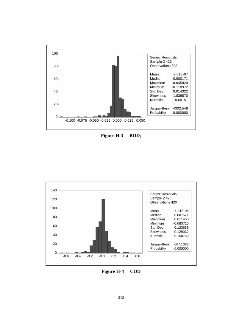
212
0
20
40
60
80
100
-0.100 -0.075 -0.050 -0.025 0.000 0.025 0.050
Series: ResidualsSample 2 423Observations 398
Mean 2.81E-07Median -0.000171Maximum 0.045824Minimum -0.118972Std. Dev. 0.014322Skewness -1.839870Kurtosis 18.68151
Jarque-Bera 4302.549Probability 0.000000
Figure H-3 BOD5
0
20
40
60
80
100
120
140
-0.6 -0.4 -0.2 -0.0 0.2 0.4 0.6
Series: ResidualsSample 2 423Observations 420
Mean 4.31E-08Median 0.007571Maximum 0.611450Minimum -0.683710Std. Dev. 0.123638Skewness -0.129032Kurtosis 9.168759
Jarque-Bera 667.1032Probability 0.000000
Figure H-4 COD

213
0
40
80
120
160
-0.4 -0.2 -0.0 0.2 0.4
Series: ResidualsSample 2 423Observations 404
Mean -1.85E-08Median 0.002795Maximum 0.462034Minimum -0.533983Std. Dev. 0.075774Skewness -0.251642Kurtosis 13.43955
Jarque-Bera 1838.832Probability 0.000000
Figure H-5 Total Carbon
0
20
40
60
80
100
120
140
-0.20 -0.15 -0.10 -0.05 0.00 0.05 0.10 0.15
Series: ResidualsSample 2 423Observations 402
Mean 9.16E-09Median 0.001865Maximum 0.151029Minimum -0.196607Std. Dev. 0.026178Skewness -0.788776Kurtosis 15.21966
Jarque-Bera 2542.795Probability 0.000000
Figure H-6 Dissolved Total Carbon

214
0
20
40
60
80
-0.0050 -0.0025 0.0000 0.0025
Series: ResidualsSample 2 423Observations 351
Mean 2.32E-09Median -6.43E-06Maximum 0.004458Minimum -0.005496Std. Dev. 0.001036Skewness -0.792611Kurtosis 8.831761
Jarque-Bera 534.1395Probability 0.000000
Figure H-7 Nitrate
0
20
40
60
80
100
120
140
-0.00375 -0.00250 -0.00125 0.00000 0.00125 0.00250
Series: ResidualsSample 2 423Observations 411
Mean 8.33E-09Median 1.34E-05Maximum 0.002629Minimum -0.003558Std. Dev. 0.000526Skewness 0.046889Kurtosis 11.88148
Jarque-Bera 1350.982Probability 0.000000
Figure H-8 Total Phosphorus

215
0
20
40
60
80
100
-0.02 -0.01 -0.00 0.01 0.02
Series: ResidualsSample 2 419Observations 263
Mean -2.49E-08Median 0.000149Maximum 0.024991Minimum -0.024298Std. Dev. 0.005338Skewness -0.159615Kurtosis 8.530587
Jarque-Bera 336.3035Probability 0.000000
Figure H-9 Oil and Grease
0
50
100
150
200
-0.00050 -0.00025 0.00000 0.00025 0.00050
Series: ResidualsSample 2 423Observations 398
Mean 1.32E-10Median -4.80E-06Maximum 0.000643Minimum -0.000509Std. Dev. 8.07E-05Skewness 0.990214Kurtosis 21.11851
Jarque-Bera 5509.022Probability 0.000000
Figure H-10 Copper

216
0
20
40
60
80
100
-0.025 0.000 0.025
Series: ResidualsSample 2 423Observations 399
Mean 9.01E-11Median -8.52E-05Maximum 0.046277Minimum -0.038511Std. Dev. 0.008340Skewness -0.094315Kurtosis 9.803021
Jarque-Bera 770.0147Probability 0.000000
Figure H-11 Iron
0
20
40
60
80
100
120
140
-0.002 -0.001 0.000 0.001 0.002
Series: ResidualsSample 68 423Observations 319
Mean 1.35E-09Median -1.49E-05Maximum 0.002630Minimum -0.001919Std. Dev. 0.000399Skewness 0.118797Kurtosis 14.72065
Jarque-Bera 1826.676Probability 0.000000
Figure H-12 Lead

217
0
20
40
60
80
100
120
140
-0.0025 0.0000 0.0025 0.0050
Series: ResidualsSample 2 423Observations 399
Mean 3.51E-10Median -3.65E-05Maximum 0.005968Minimum -0.003714Std. Dev. 0.000661Skewness 2.024230Kurtosis 25.15788
Jarque-Bera 8434.885Probability 0.000000
Figure H-13 Zinc

218

219
Appendix IRegression Results
-0.2
0
0.2
0.4
0.6
0.8
1
1.2
0 0.2 0.4 0.6 0.8 1 1.2
Observed Load (g/m2)
Pre
dic
ted
Lo
ad (
g/m
)
(a) Fit of Data from West 35th Street Site
VSS
-0.6
-0.5
-0.4
-0.3
-0.2
-0.1
0
0.1
0.2
0.3
0.4
0 5 10 15 20 25 30 35
Total Rainfall (mm)
Res
idu
al (
g/m
)
(b) Model Residuals vs. Total Rainfall (Dashed Lines Indicate ± 2 Std. Error)
Figure I-1 VSS Model Results

220
-0.2
0
0.2
0.4
0.6
0.8
1
1.2
0 0.2 0.4 0.6 0.8 1 1.2
Observed Load (g/m2)
Pre
dic
ted
Lo
ad (
g/m
)
Observed
35th St.
Convict Hill
(a) Model Predictions at the Convict Hill Site
VSS
-0.7
-0.6
-0.5
-0.4
-0.3
-0.2
-0.1
0
0.1
0.2
0.3
0.4
0 5 10 15 20 25 30 35
Total Rainfall (mm)
Res
idu
al (
g/m
)
35th St. Convict Hill
(b) Prediction Error vs. Total Rainfall
Figure I-2 VSS Model Predictions

221
-0.05
0
0.05
0.1
0.15
0.2
0.25
0.3
0 0.05 0.1 0.15 0.2 0.25 0.3
Observed Load (g/m2)
Pre
dic
ted
Lo
ad (
g/m
)
(a) Fit of Data from West 35th Street Site
BOD5
-0.12
-0.1
-0.08
-0.06
-0.04
-0.02
0
0.02
0.04
0.06
0 5 10 15 20 25 30 35
Total Rainfall (mm)
Res
idu
al (
g/m
)
(b) Model Residuals vs. Total Rainfall (Dashed Lines Indicate ± 2 Std. Error)
Figure I-3 BOD5 Model Results

222
-0.05
0
0.05
0.1
0.15
0.2
0.25
0.3
0 0.05 0.1 0.15 0.2 0.25 0.3
Observed Load (g/m2)
Pre
dic
ted
Lo
ad (
g/m
)
Observed
35th St.
Convict Hill
(a) Model Predictions at the Convict Hill Site
BOD5
-0.12
-0.1
-0.08
-0.06
-0.04
-0.02
0
0.02
0.04
0.06
0 5 10 15 20 25 30 35Total Rainfall (mm)
Res
idu
al (
g/m
)
35th St. Convict Hill
(b) Prediction Error vs. Total Rainfall
Figure I-4 BOD5 Model Predictions

223
-0.5
0
0.5
1
1.5
2
0 0.5 1 1.5 2
Observed Load (g/m2)
Pre
dic
ted
Lo
ad (
g/m
)
(a) Fit of Data from West 35th Street Site
Total Carbon
-0.6
-0.5
-0.4
-0.3
-0.2
-0.1
0
0.1
0.2
0.3
0.4
0.5
0 5 10 15 20 25 30 35
Total Rainfall (mm)
Res
idu
al (
g/m
)
(b) Model Residuals vs. Total Rainfall (Dashed Lines Indicate ± 2 Std. Error)
Figure I-5 Total Carbon Model Results

224
-0.5
0
0.5
1
1.5
2
0 0.5 1 1.5 2
Observed Load (g/m2)
Pre
dic
ted
Lo
ad (
g/m
)Observed
35th St.
Convict Hill
(a) Model Predictions at the Convict Hill Site
Total Carbon
-0.6
-0.5
-0.4
-0.3
-0.2
-0.1
0
0.1
0.2
0.3
0.4
0.5
0 5 10 15 20 25 30 35
Total Rainfall (mm)
Res
idu
al (
g/m
)
35th St. Convict Hill
(b) Prediction Error vs. Total Rainfall
Figure I-6 Total Carbon Model Predictions

225
0
0.05
0.1
0.15
0.2
0.25
0.3
0.35
0.4
0.45
0.5
0 0.05 0.1 0.15 0.2 0.25 0.3 0.35 0.4 0.45 0.5
Observed Load (g/m2)
Pre
dic
ted
Lo
ad (
g/m
)
(a) Fit of Data from West 35th Street Site
Dissolved Total Carbon
-0.2
-0.15
-0.1
-0.05
0
0.05
0.1
0.15
0.2
0 5 10 15 20 25 30 35
Total Rainfall (mm)
Res
idu
al (
g/m
)
(b) Model Residuals vs. Total Rainfall (Dashed Lines Indicate ± 2 Std. Error)
Figure I-7 Dissolved Total Carbon Model Results

226
-0.05
0
0.05
0.1
0.15
0.2
0.25
0.3
0.35
0.4
0.45
0.5
0 0.05 0.1 0.15 0.2 0.25 0.3 0.35 0.4 0.45 0.5
Observed Load (g/m2)
Pre
dic
ted
Lo
ad (
g/m
)Observed
35th St.
Convict Hill
(a) Model Predictions at the Convict Hill Site
Dissolved Total Carbon
-0.2
-0.15
-0.1
-0.05
0
0.05
0.1
0.15
0.2
0 5 10 15 20 25 30 35
Total Rainfall (mm)
Res
idu
al (
g/m
)
35th St. Convict Hill
(b) Prediction Error vs. Total Rainfall
Figure I-8 Dissolved Total Carbon Model Predictions

227
-0.001
0
0.001
0.002
0.003
0.004
0.005
0.006
0.007
0.008
0 0.001 0.002 0.003 0.004 0.005 0.006 0.007 0.008
Observed Load (g/m2)
Pre
dic
ted
Lo
ad (
g/m
)
(a) Fit of Data from West 35th Street Site
Total Phosphorus
-0.004
-0.003
-0.002
-0.001
0
0.001
0.002
0.003
0 5 10 15 20 25 30 35
Total Rainfall (mm)
Res
idu
al (
g/m
)
(b) Model Residuals vs. Total Rainfall (Dashed Lines Indicate ± 2 Std. Error)
Figure I-9 Total Phosphorus Model Results

228
-0.001
0
0.001
0.002
0.003
0.004
0.005
0.006
0.007
0.008
0 0.001 0.002 0.003 0.004 0.005 0.006 0.007 0.008
Observed Load (g/m2)
Pre
dic
ted
Lo
ad (
g/m
)Observed
35th St.
Convict Hill
(a) Model Predictions at the Convict Hill Site
Total Phosphorus
-0.004
-0.003
-0.002
-0.001
0
0.001
0.002
0.003
0 5 10 15 20 25 30 35
Total Rainfall (mm)
Res
idu
al (
g/m
)
35th St. Convict Hill
(b) Prediction Error vs. Total Rainfall
Figure I-10 Total Phosphorus Model Predictions

229
-0.02
0
0.02
0.04
0.06
0.08
0.1
0.12
0 0.02 0.04 0.06 0.08 0.1 0.12
Observed Load (g/m2)
Pre
dic
ted
Lo
ad (
g/m
)
(a) Fit of Data from West 35th Street Site
Oil & Grease
-0.025
-0.02
-0.015
-0.01
-0.005
0
0.005
0.01
0.015
0.02
0.025
0 5 10 15 20 25 30 35
Total Rainfall (mm)
Res
idu
als
(g/m
)
(b) Model Residuals vs. Total Rainfall (Dashed Lines Indicate ± 2 Std. Error)
Figure I-11 Oil and Grease Model Results

230
-0.02
0
0.02
0.04
0.06
0.08
0.1
0.12
0 0.02 0.04 0.06 0.08 0.1 0.12
Observed Load (g/m2)
Pre
dic
ted
Lo
ad (
g/m
)Observed
35th St.
Convict Hill
(a) Model Predictions at the Convict Hill Site
Oil & Grease
-0.03
-0.02
-0.01
0
0.01
0.02
0.03
0 5 10 15 20 25 30 35
Total Rainfall (mm)
Res
idu
al (
g/m
)
35th St. Convict Hill
(b) Prediction Error vs. Total Rainfall
Figure I-12 Oil and Grease Model Predictions

231
-0.0005
0
0.0005
0.001
0.0015
0.002
0.0025
0 0.0005 0.001 0.0015 0.002 0.0025
Observed Load (g/m2)
Pre
dic
ted
Lo
ad (
g/m
)
(a) Fit of Data from West 35th Street Site
Copper
-6.00E-04
-4.00E-04
-2.00E-04
0.00E+00
2.00E-04
4.00E-04
6.00E-04
8.00E-04
0 5 10 15 20 25 30 35Total Rainfall (mm)
Res
idu
al (
g/m
)
(b) Model Residuals vs. Total Rainfall (Dashed Lines Indicate ± 2 Std. Error)
Figure I-13 Copper Model Results

232
-0.0005
0
0.0005
0.001
0.0015
0.002
0.0025
0 0.0005 0.001 0.0015 0.002 0.0025
Observed Load (g/m2)
Pre
dic
ted
Lo
ad (
g/m
)Observed
35th St.
Convict Hill
(a) Model Predictions at the Convict Hill Site
Copper
-6.00E-04
-4.00E-04
-2.00E-04
0.00E+00
2.00E-04
4.00E-04
6.00E-04
8.00E-04
0 5 10 15 20 25 30 35
Total Rainfall (mm)
Res
idu
al (
g/m
)
35th St. Convict Hill
(b) Prediction Error vs. Total Rainfall
Figure I-14 Copper Model Predictions

233
-0.04
-0.02
0
0.02
0.04
0.06
0.08
0.1
0.12
0.14
0 0.02 0.04 0.06 0.08 0.1 0.12 0.14
Observed Load (g/m2)
Pre
dic
ted
Lo
ad (
g/m
)
(a) Fit of Data from West 35th Street Site
Iron
-0.04
-0.03
-0.02
-0.01
0
0.01
0.02
0.03
0.04
0.05
0 5 10 15 20 25 30 35
Total Rainfall (mm)
Res
idu
al (
g/m
)
(b) Model Residuals vs. Total Rainfall (Dashed Lines Indicate ± 2 Std. Error)
Figure I-15 Iron Model Results

234
-0.04
-0.02
0
0.02
0.04
0.06
0.08
0.1
0.12
0.14
0 0.02 0.04 0.06 0.08 0.1 0.12 0.14
Observed Load (g/m2)
Pre
dic
ted
Lo
ad (
g/m
)Observed
35th St.
Convict Hill
(a) Model Predictions at the Convict Hill Site
Iron
-0.06
-0.05
-0.04
-0.03
-0.02
-0.01
0
0.01
0.02
0.03
0.04
0.05
0 5 10 15 20 25 30 35
Total Rainfall (mm)
Res
idu
al (
g/m
)
35th St. Convict Hill
(b) Prediction Error vs. Total Rainfall
Figure I-16 Iron Model Predictions

235
-0.002
-0.001
0
0.001
0.002
0.003
0.004
0 0.001 0.002 0.003 0.004
Observed Load (g/m2)
Pre
dic
ted
Lo
ad (
g/m
)
(a) Fit of Data from West 35th Street Site
Lead
-0.002
-0.0015
-0.001
-0.0005
0
0.0005
0.001
0.0015
0.002
0.0025
0.003
0 5 10 15 20 25 30 35
Total Rainfall (mm)
Res
idu
al (
g/m
)
(b) Model Residuals vs. Total Rainfall (Dashed Lines Indicate ± 2 Std. Error)
Figure I-17 Lead Model Results

236
-0.002
-0.001
0
0.001
0.002
0.003
0.004
0 0.001 0.002 0.003 0.004
Observed Load (g/m2)
Pre
dic
ted
Lo
ad (
g/m
)Observed
35th St.
Convict Hill
(a) Model Predictions at the Convict Hill Site
Lead
-0.002
-0.0015
-0.001
-0.0005
0
0.0005
0.001
0.0015
0.002
0.0025
0.003
0 5 10 15 20 25 30 35
Total Rainfall (mm)
Res
idu
al (
g/m
)
35th St. Convict Hill
(b) Prediction Error vs. Total Rainfall
Figure I-18 Lead Model Predictions