technical report - nsk-literature.com

TECHNICAL REPORT

SUBSCRIBE TO NSK NEWSLETTERSUBSCRIBE TO NSK NEWSLETTER

http://www.nsk-literature.com/subscribe

1. ISO Dimensional system and bearing numbers 1.1 ISO Dimensional system …………………………………………………………… 6 1.2 Formulation of bearing numbers …………………………………………………… 8 1.3 Bearing numbers for tapered roller bearings (inch system) ………………… 10 1.4 Bearing numbers for miniature ball bearings ………………………………… 12 1.5 Auxiliary bearing symbols ……………………………………………………… 14

2. Dynamic load rating, fatigue life, and static load rating 2.1 Dynamic load rating ……………………………………………………………… 18 2.2 Dynamic equivalent load ………………………………………………………… 22 2.3 Dynamic equivalent load of triplex angular contact ball bearings …………… 24 2.4 Average of fluctuating load and speed ………………………………………… 26 2.5 Combination of rotating and stationary loads ………………………………… 28 2.6 Life calculation of multiple bearings as a group ……………………………… 30 2.7 Load factor and fatigue life by machine ……………………………………… 32 2.8 Radial clearance and fatigue life ………………………………………………… 34 2.9 Misalignment of inner/outer rings and fatigue life of deep-groove ball bearings ……………………………………………………………………… 36 2.10 Misalignment of inner/outer rings and fatigue life of cylindrical roller bearings …………………………………………………………………… 38 2.11 Fatigue life and reliability ………………………………………………………… 40 2.12 Oil film parameters and rolling fatigue life ……………………………………… 42 2.13 EHL oil film parameter calculation diagram …………………………………… 44 2.13.1　Oil film parameter …………………………………………………………… 44 2.13.2　Oil film parameter calculation diagram …………………………………… 44 2.13.3　Effect of oil shortage and shearing heat generation ……………………… 48 2.14 Fatigue analysis …………………………………………………………………… 50 2.14.1　Measurement of fatigue degree …………………………………………… 50 2.14.2　Surface and sub-surface fatigues ………………………………………… 52 2.14.3　Analysis of practical bearing (1) …………………………………………… 54 2.14.4　Analysis of practical bearing (2) …………………………………………… 56 2.15 Conversion of dynamic load rating with reference to life at 500 min–1 and 3 000 hours ……………………………………………………………………… 58 2.16 Basic static load ratings and static equivalent loads ………………………… 60

3. Bearing fitting practice 3.1 Load classifications ……………………………………………………………… 62 3.2 Required effective interference due to load …………………………………… 64 3.3 Interference deviation due to temperature rise (aluminum housing, plastic housing) …………………………………………… 66 3.4 Fit calculation ……………………………………………………………………… 68 3.5 Surface pressure and maximum stress on fitting surfaces ………………… 70 3.6 Mounting and withdrawal loads ………………………………………………… 72 3.7 Tolerances for bore diameter and outside diameter ………………………… 74

CONTENTSPages

3.8 Interference and clearance for fitting (shafts and inner rings) ……………… 76 3.9 Interference and clearance for fitting (housing holes and outer rings) ……… 78 3.10 Interference dispersion (shafts and inner rings) ……………………………… 80 3.11 Interference dispersion (housing bores and outer rings) …………………… 82 3.12 Fits of four-row tapered roller bearings (metric) for roll necks ……………… 84

4. Internal clearance 4.1 Internal clearance ………………………………………………………………… 86 4.2 Calculating residual internal clearance after mounting ……………………… 88 4.3 Effect of interference fit on bearing raceways (fit of inner ring) …………… 90 4.4 Effect of interference fit on bearing raceways (fit of outer ring) …………… 92 4.5 Reduction in radial internal clearance caused by a temperature difference between inner and outer rings ……………………………………… 94 4.6 Radial and axial internal clearances and contact angles for single row deep groove ball bearings ……………………………………………………… 96 4.6.1　Radial and axial internal clearances ………………………………………… 96 4.6.2　Relation between radial clearance and contact angle …………………… 98 4.7 Angular clearances in single-row deep groove ball bearings ………………… 100 4.8 Relationship between radial and axial clearances in double-row angular contact ball bearings …………………………………………………………… 102 4.9 Angular clearances in double-row angular contact ball bearings …………… 104 4.10 Measuring method of internal clearance of combined tapered roller bearings (offset measuring method) …………………………………… 106 4.11 Internal clearance adjustment method when mounting a tapered roller bearing …………………………………………………………………………… 108

5. Bearing internal load distribution and displacement 5.1 Bearing internal load distribution ……………………………………………… 110 5.2 Radial clearance and load factor for radial ball bearings …………………… 112 5.3 Radial clearance and maximum rolling element load ………………………… 114 5.4 Contact surface pressure and contact ellipse of ball bearings under pure radial loads ………………………………………………………………… 116 5.5 Contact surface pressure and contact area under pure radial load (roller bearings) …………………………………………………………………… 120 5.6 Rolling contact trace and load conditions …………………………………… 128 5.6.1　Ball bearing …………………………………………………………………… 128 5.6.2　Roller bearing …………………………………………………………………… 130 5.7 Radial load and displacement of cylindrical roller bearings ………………… 132 5.8 Misalignment, maximum rolling-element load and moment for deep groove ball bearings ……………………………………………………… 134 5.8.1　Misalignment angle of rings and maximum rolling-element load ………… 134 5.8.2　Misalignment of inner and outer rings and moment ……………………… 136 5.9 Load distribution of single-direction thrust bearing due to eccentric load …………………………………………………………………… 138

Pages

6. Preload and axial displacement 6.1 Position preload and constant-pressure preload ……………………………… 140 6.2 Load and displacement of position-preloaded bearings ……………………… 142 6.3 Average preload for duplex angular contact ball bearings …………………… 150 6.4 Axial displacement of deep groove ball bearings …………………………… 156 6.5 Axial displacement of tapered roller bearings ………………………………… 160

7. Starting and running torques 7.1 Preload and starting torque for angular contact ball bearings ……………… 162 7.2 Preload and starting torque for tapered roller bearings ……………………… 164 7.3 Empirical equations of running torque of high-speed ball bearings ………… 166 7.4 Empirical equations for running torque of tapered roller bearings ………… 168

8. Bearing type and allowable axial load 8.1 Change of contact angle of radial ball bearings and allowable axial load ………………………………………………………………………………… 172 8.1.1　Change of contact angle due to axial load ………………………………… 172 8.1.2　Allowable axial load for a deep groove ball bearing ……………………… 176 8.2 Allowable axial load (break down strength of the ribs) for a cylindrical roller bearings …………………………………………………………………… 178

9. Lubrication 9.1 Lubrication amount for the forced lubrication method ……………………… 180 9.2 Grease filling amount of spindle bearing for machine tools ………………… 182 9.3 Free space and grease filling amount for deepgroove ball bearings ……… 184 9.4 Free space of angular contact ball bearings ………………………………… 186 9.5 Free space of cylindrical roller bearings ……………………………………… 188 9.6 Free space of tapered roller bearings ………………………………………… 190 9.7 Free space of spherical roller bearings ………………………………………… 192 9.8 NSK’s dedicated greases ……………………………………………………… 194 9.8.1　NS7 and NSC greases for induction motor bearings ……………………… 194 9.8.2　ENS and ENR greases for high-temperature/speed ball bearings ……… 196 9.8.3　EA3 and EA6 greases for commutator motor shafts ……………………… 198 9.8.4　WPH grease for water pump bearings ……………………………………… 200 9.8.5　MA7 and MA8 greases for automotive electric accessory bearings ……… 202

10. Bearing materials 10.1 Comparison of national standards of rolling bearing steel …………………… 204 10.2 Long life bearing steel (NSK Z steel) ………………………………………… 206 10.3 High temperature bearing materials …………………………………………… 208 10.4 Dimensional stability of bearing steel …………………………………………… 210 10.5 Characteristics of bearing and shaft/housing materials ……………………… 212 10.6 Engineering ceramics as bearing material……………………………………… 214 10.7 Physical properties of representative polymers used as bearing material … 218

Pages

10.8 Characteristics of nylon material for cages …………………………………… 220 10.9 Heat-resistant resin materials for cages ……………………………………… 222 10.10 Features and operating temperature range of ball bearing seal material … 224

11. Load calculation of gears 11.1 Calculation of loads on spur, helical, and double-helical gears …………… 226 11.2 Calculation of load acting on straight bevel gears …………………………… 230 11.3 Calculation of load on spiral bevel gears ……………………………………… 232 11.4 Calculation of load acting on hypoid gears …………………………………… 234 11.5 Calculation of load on worm gear ……………………………………………… 238

12. General miscellaneous information 12.1 JIS concerning rolling bearings ………………………………………………… 240 12.2 Amount of permanent deformation at point where inner and outer rings contact the rolling element ………………………………………… 242 12.2.1　Ball bearings ………………………………………………………………… 242 12.2.2　Roller bearings ……………………………………………………………… 244 12.3 Rotation and revolution speed of rolling element …………………………… 248 12.4 Bearing speed and cage slip speed …………………………………………… 250 12.5 Centrifugal force of rolling elements …………………………………………… 252 12.6 Temperature rise and dimensional change …………………………………… 254 12.7 Bearing volume and apparent specific gravity ………………………………… 256 12.8 Projection amount of cage in tapered roller bearing ………………………… 258 12.9 Natural frequency of individual bearing rings ………………………………… 260 12.10 Vibration and noise of bearings ………………………………………………… 262 12.11 Application of FEM to design of bearing system …………………………… 264

13. NSK Special bearings 13.1 Ultra-precision ball bearings for gyroscopes ………………………………… 268 13.2 Bearings for vacuum use — ball bearings for X-ray tube — ……………… 274 13.3 Ball bearing for high vacuum …………………………………………………… 278 13.4 Light-contact-sealed ball bearings ……………………………………………… 280 13.5 Bearing with integral shaft ……………………………………………………… 282 13.6 Bearings for electromagnetic clutches in car air-conditioners ……………… 284 13.7 Sealed clean bearings for transmissions ……………………………………… 288 13.8 Double-row cylindrical roller bearings, NN30 T series (with polyamide resin cage) …………………………………………………… 290 13.9 Single-row cylindrical roller bearings, N10B T series (cage made of polyamide resin) ……………………………………………… 292 13.10 Sealed clean bearings for rolling mill roll neck ………………………………… 294 13.11 Bearings for chain conveyors …………………………………………………… 296 13.12 RCC bearings for railway rolling stock ………………………………………… 300

Pages

6

1. ISO Dimensional system and bearing numbers

1.1 ISO Dimensional system

The boundary dimensions of rolling bearings, namely, bore diameter, outside diameter, width, and chamfer dimensions have been standardized so that common dimensions can be adopted on a worldwide scale. In Japan, JIS (Japan Industrial Standard) adheres to the boundary dimensions established by ISO. ISO is a French acronym which is translated into English as the International Organization for Standardization. The ISO dimensional system specifies the following dimensions for rolling bearings: bore diameter, d, outside diameter, D, width, B, (or height, T) and chamfer dimension, r, and provides for the diameter to range from a bore size of 0.6 mm to an outside diameter of 2500 mm. In addition, a method to expand the range is laid out so that the bore diameter, d, (d>500 mm) is taken from the geometrical ratio standard R40.

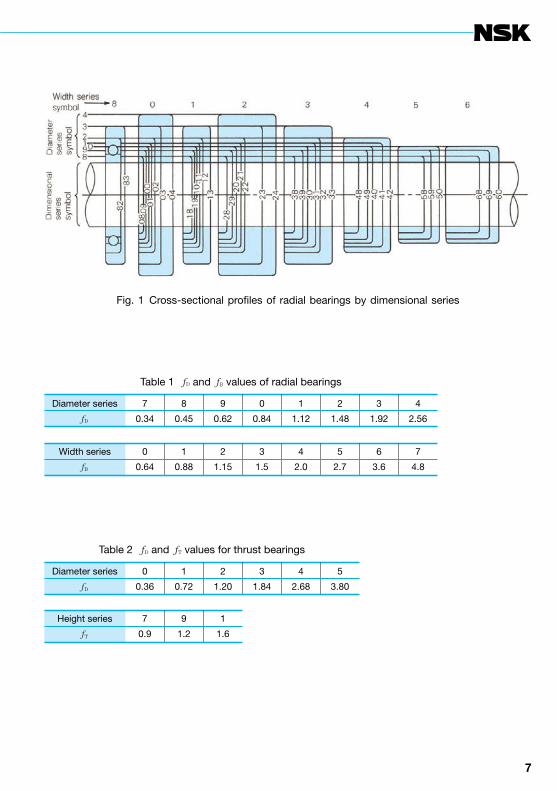
When expanding the dimensional system, the equation for the outside diameter equals D=d+ fDd0.9 and the width equals B= fB · (D–d)/2. Both of these are to be used for radial bearings. Dimensions of the width, B, if possible, should be taken from numerical sequence R80 of preferred numbers in JIS Z 8601. The values of factors fD and fB are respectively specified for the diameter series and width series in Table 1. Minimum chamfer dimension, rs min, should be selected from ISO table and in principle be that value which is nearest to, but not larger than 7% of the bearing width, B, or of the sectional height (D–d)/2, whichever is the smaller. Rounding-off of fractions has been specified for the above dimensions.

The outside diameter can be obtained from the factor fD in Table 1 and bore d. Incidentally, the diameter series symbols 9, 0, 2, 3 are used most often. The thickness between the bore and outside diameters is determined by the diameter series. The outside diameter series increases in the order of 7, 8, 9, 0, 1, 2, 3, and 4 (Fig. 1) while the bore size remains the same size. The diameter series are combined with the factor fB and classified into a few different width series. The dimension series is composed of combinations of the width series and diameter

series.In the United States, many tapered roller

bearings are expressed in the inch system rather than the metric system as specified by ISO. Japan and European countries use the metric system which is in accordance with ISO directives.

The expansion of thrust bearings series (single-direction with flat seats) is laid out in a similar manner as the radial bearings with the boundary dimensions as follows: outside diameter, D=d+ f Dd0.8, and height, T= fT · (D–d)/2. Minimum chamfer dimension, rs min, should be selected from ISO table and in principle be that value which is nearest to, but not larger than 7% of the bearing height, T, or (D–d)/2, whichever is the smaller. Values for the factors fD and fT are as shown in Table 2.

6 7

Table 1 fD and fB values of radial bearings

Diameter series 7 8 9 0 1 2 3 4

fD 0.34 0.45 0.62 0.84 1.12 1.48 1.92 2.56

Width series 0 1 2 3 4 5 6 7

fB 0.64 0.88 1.15 1.5 2.0 2.7 3.6 4.8

Table 2 fD and fT values for thrust bearings

Diameter series 0 1 2 3 4 5

fD 0.36 0.72 1.20 1.84 2.68 3.80

Height series 7 9 1

fT 0.9 1.2 1.6

Fig. 1　Cross-sectional profiles of radial bearings by dimensional series

8

ISO Dimensional system and bearing numbers

1.2 Formulation of bearing numbers

The rolling bearing is an important machine element and its boundary dimensions have been internationally standardized. International standardization of bearing numbers has been examined by ISO but not adopted. Now, manufacturers of various countries are using their own bearing numbers. Japanese manufacturers express the bearing number with 4 or 5 digits by a system which is mainly based on the SKF bearing numbers. The JIS has specified bearing numbers for some of the more commonly used bearings.A bearing number is composed as follows.

The width series symbol and diameter series symbol are combined and called the dimensional series symbol. For radial bearings, the outside diameter increases with the diameter series symbols 7, 8, 9, 0, 1, 2, 3, and 4. Usually, 9, 0, 2, and 3 are the most frequently used. Width series symbols include 0, 1, 2, 3, 4, 5, and 6 and these are combined with the respective diameter series symbols. Among the width series symbols, 0, 1, 2, and 3 are the most frequently used. Width series symbols become wider in this ordering system to match the respective diameter series symbol.

For standard radial ball bearings, the width series symbol is omitted and the bearing number is expressed by 4 digits. Also, it is common practice to omit the width series symbol of the zero for cylindrical roller bearings.

For thrust bearings, there are various combinations between the diameter symbols and height symbols (thrust bearings use the term height symbol rather than width symbol).

The bore diameter symbol is a number which is 1/5 of the bore diameter dimension when bores are 20 mm or greater. For instance, if the bore diameter is 30 mm then the bore diameter symbol is 06. However, when the bore diameter dimension is less than 17 mm, then the bore diameter symbol is by common practice taken from Table 1. Although bearing numbers vary depending on the country, many manufacturers follow this rule when formulating bore symbols.

Numbers and letters are used to form symbols to designate a variety of types and sizes of bearings. For instance, cylindrical roller bearings use letters such as N, NU, NF, NJ and so forth to indicate various roller guide rib positions. The formulation of a bearing number is shown in Table 2.

Bore No.Bore diameter d

（mm（

/0.6( 1)（1

/1.5( 1)（2

/2.5( 1)（3（4（5（6（7（8（9

00010203

0.6 1 1.5 2 2.5 3 4 5 6 7 8 9 10 12 15 17

Notes( 1)（NSK 0.6 mmbore bearing is notavailable. 1X and2X are used for theNSK bearingnumber instead of/1.5 and /2.5respectilely.

Table 1

○ ○ ○ ○ ○

Bore number

Diameter seriessymbol

Width seriessymbol

Type symbol

Dimensionalseries symbol

Bearingseries symbol

8 9

Table 2 Formulation of a bearing number

Bearing types Samplebrg Type No. Width or height(1)

series No.Dia. Series

No. Bore No.

Radialballbearing

Single-row deep groove type

629 6 [0] omitted 2 9

60106303

66

[1] omitted[0] omitted

03

1003

Single-row angular type 7215A 7 [0] omitted 2 15

Double-row angular type32065312

35


23

0612

Double-row self-aligning type12052211

12


22

0511

Radialrollerbearing

Cylindrical roller

NU 1016N 220

NU 2224NN 3016

NUN

NUNN

1[0] omitted23

0220

16202416

Tapered roller 30214 3 0 2 14

Spherical roller 23034 2 3 0 34

Thrustballbearing

Single-direction flat seatsDouble-direction flat seatsSingle-direction self-aligning seatsDouble-direction self-aligning seats

51124523125331854213

5555

123(2)4(2)

1332

24121813

Thrustrollerbearing

Spherical thrust roller 29230 2 9 2 30

Notes ( 1)（Height symbol is used for thrust bearings instead of width. ( 2)（These express a type symbol rather than a height symbol.

10


1.3 Bearing numbers for tapered roller bearings (Inch system)

The ABMA (The American Bearing Manufacturers Association) standard specifies how to formulate the bearing number for tapered roller bearings in the inch system. The ABMA method of specifying bearing numbers is applicable to bearings with new designs. Bearing numbers for tapered roller bearings in the inch system, which have been widely used, will continue to be used and known by the same bearing numbers. Although TIMKEN uses ABMA bearing numbers to designate new bearing designs, many of its bearing numbers do not conform to ABMA rules.

Tapered roller bearings (Inch system)The outer ring of a tapered roller bearing is

called a “CUP” and the inner ring is a “CONE”. A CONE ASSEMBLY consists of tapered rollers, cage and inner ring, though sometimes it is called a “CONE” instead of “CONE ASSEMBLY”. Therefore, an inch-system tapered roller bearing consists of one CUP and one CONE (exactly speaking, one CONE ASSEMBLY). Each part is sold separately. Therefore, to obtain a complete set both parts must be ordered.

In the example of page 11, LM11949 is only a CONE. A complete inch-system tapered roller bearing is called a CONE/CUP and is specified by LM11949/LM11910 for this example.

A bearing number is composed as follows.

“ A ” indicates an alphabetical character.“（” indicates a numerical digit.

Load limit symbol

Contact angle number

Series number

Auxiliary number

Auxiliary symbol

AA （（（（（（ AA

10 11

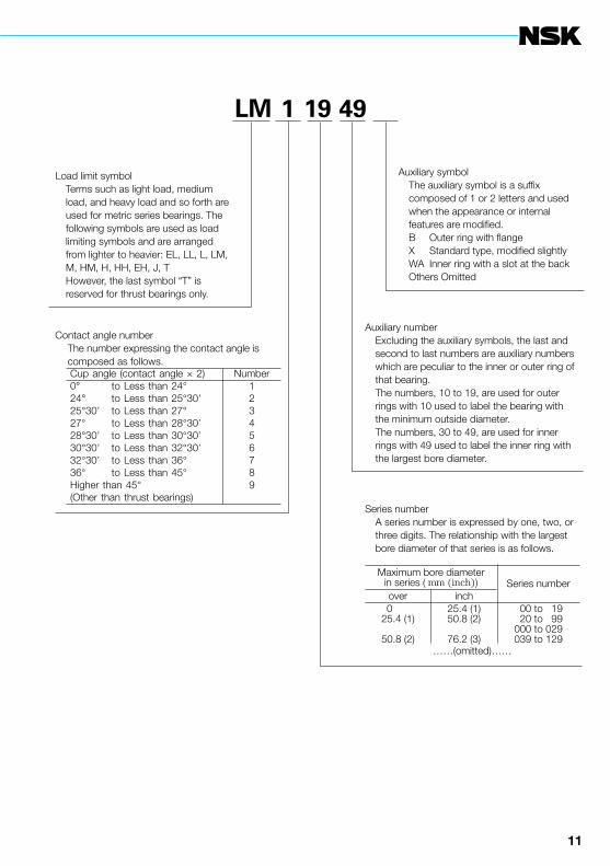
LM　1　19　49　

Contact angle numberThe number expressing the contact angle is composed as follows.

Auxiliary symbolThe auxiliary symbol is a suffix composed of 1 or 2 letters and used when the appearance or internal features are modified.B Outer ring with flangeX Standard type, modified slightlyWA Inner ring with a slot at the backOthers Omitted

Load limit symbolTerms such as light load, medium load, and heavy load and so forth are used for metric series bearings. The following symbols are used as load limiting symbols and are arranged from lighter to heavier: EL, LL, L, LM, M, HM, H, HH, EH, J, T However, the last symbol “T” is reserved for thrust bearings only.

Cup angle (contact angle × 2) Number 0° to Less than 24° 1 24° to Less than 25°30’ 2 25°30’ to Less than 27° 3 27° to Less than 28°30’ 4 28°30’ to Less than 30°30’ 5 30°30’ to Less than 32°30’ 6 32°30’ to Less than 36° 7 36° to Less than 45° 8 Higher than 45° 9 (Other than thrust bearings)

Auxiliary numberExcluding the auxiliary symbols, the last and second to last numbers are auxiliary numbers which are peculiar to the inner or outer ring of that bearing.The numbers, 10 to 19, are used for outer rings with 10 used to label the bearing with the minimum outside diameter.The numbers, 30 to 49, are used for inner rings with 49 used to label the inner ring with the largest bore diameter.

Series numberA series number is expressed by one, two, or three digits. The relationship with the largest bore diameter of that series is as follows.

Maximum bore diameter in series ( mm (inch))over inch

0　　 25.4 (1) 00 to 19 25.4 (1) 50.8 (2) 20 to 99 000 to 029 50.8 (2) 76.2 (3) 039 to 129

……(omitted)……

Series number

12


1.4 Bearing numbers for miniature ball bearings

Ball bearings with outside diameters below 9 mm (or below 9.525 mm for bearings in the inch design) are called miniature ball bearings and are mainly used in VCRs, computer peripherals, various instruments, gyros, micro-motors, etc. Ball bearings with outside diameters greater than or equal to 9 mm (greater than or equal to 9.525 mm for inch design bearings) and bore diameters less than 10 mm are called extra-small ball bearings.

As in general bearings, special capabilities of miniature ball bearings are expressed by descriptive symbols added after the basic bearing number. However, one distinction of miniature and extra-small ball bearings is that a clearance indicating symbol is always included and a torque symbol is often included even if the frictional torque is quite small.

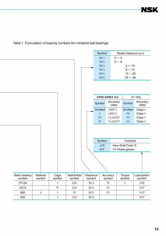
NSK has established a clearance system for miniature and extra-small ball bearings with 6 gradations of clearance so that NSK can satisfy the clearance demands of its customers. The MC3 clearance is the normal clearance suitable for general bearings.

As far as miniature and extra-small ball bearings are concerned, the ISO standards are applied to bearings in the metric design bearings and ABMA standards are applied to inch design bearings.

Miniature ball bearings are often required to have low frictional torque when used in machines. Therefore, torque standards have been established for low frictional torque. Torque symbols are used to indicate the classification of miniature bearings within the frictional standards.

The cage, seal, and shield symbols for miniature ball bearings are the same as those used for general bearings. The material symbol indicating stainless steel is an “S” and is added before the basic bearing number in both inch and metric designs for bearings of special dimensions. However, for metric stainless steel bearings of standard dimensions, an “h” is added after the basic bearing number. The figure below shows the arrangement and

meaning and so forth of bearing symbols for miniature and extra-small ball bearings.

Classification Materialsymbol

Inch design bearings S

Special metric design bearings （

Standard metric designbearings

（

（

Symbol Contents

ZZSZZ

ShieldShield

Symbol Contents

JWT

Pressed-cageCrown type cageNon-metallic cage

Symbol Contents

OmittedhS

Bearing steel (SUJ2)Stainless steel (SUS440C)Stainless steel (SUS440C)

12 13

Basic bearingnumber

Materialsymbol

Cagesymbol

Seal/shieldsymbol

Clearancesymbol

Accuracysymbol

Torquesymbol

Lubricatdonsymbol

FR133 （ J ZZS MC4 7P L AF2

MR74 （ W ZZS MC3 P5 （ NS7

692 h J ZZ MC3 P5 （ NS7

602 （ J ZZS MC4 （（ NS7

Symbol Contents

AF2NS7

Aero-Shell Fluid 12NS Hilube grease

ANSI/ABMA Std. ISO Std.

Symbol Accuracyclass Symbol Accuracy

class

Omitted3

5P7P

ABEC1ABEC3CLASS5PCLASS7P

OmittedP6P5P4

Class 0Class 6Class 5Class 4

Symbol Radial clearance (μm)

MC1MC2MC3MC4MC5MC6

（（（（（（0 〜（5（（（（（（3 〜（8

（5 〜 10（8 〜 13

13 〜 2020 〜 28

Table 1 Formulation of bearing numbers for miniature ball bearings.

14


1.5 Auxiliary bearing symbols

Rolling bearings are provided with various capabilities to meet a variety of application demands and methods of use. These special capabilities are classified and indicated by auxiliary symbols attached after the basic bearing number. The entire system of basic and auxiliary symbols should be completely unified but this level of standardization has not been achieved.

Currently, manufacturers use a combination of their own symbols and specified symbols. The internal clearance symbols and accuracy symbols are two sets of symbols which are widely used and specified by JIS. The auxiliary symbols employed by NSK are listed in alphabetical order as follows.

Note ( 1)（Part of the basic bearing number

Symbol Contents Example

A Internal design differs from standard design6307AHR32936JA

A(1) Angular contact ball bearing with standard contact angle of α=30° 7215A

AH Removable sleeve type symbol AH3132

A5(1) Angular contact ball bearing with standard contact angle of α=25° 7913A5

BCylindrical roller bearing: the allowance of roller inscribed circle diameteror circumscribed circle diameter does not comply with JIS standards NU306B

Inch series tapered roller bearing with flanged cup 779/772B

B(1) Angular contact ball bearing with standard contact angle of α=40° 7310B

C(1)Angular contact ball bearing with standard contact angle of α=15° 7205C

Tapered roller bearing with contact angle of about 20° HR32205C

CA Spherical roller bearing with high load capacity (machined cage) 22324CA

CD Spherical roller bearing with high load capacity (pressed cage) 22228CD

C1

C2

C3

C4

C5

C1 clearance (smaller than C2)C2 clearance (smaller than normal clearance)C3 clearance (larger than normal clearance)C4 clearance (larger than C3)C5 clearance (larger than C4)

6218C3

CCCC1

CC2

CC3

CC4

CC5

Normal matched clearance of cylindrical roller bearingC1 matched clearance of cylindrical roller bearingC2 matched clearance of cylindrical roller bearingC3 matched clearance of cylindrical roller bearingC4 matched clearance of cylindrical roller bearingC5 matched clearance of cylindrical roller bearing

N238CC2

CC9 Matched clearance of cylindrical roller bearing with tapered bore (smallerthan CC1) NN3017KCC9

CG15 Special radial clearance (indicates median clearance) 6022CG15

CM Special clearances for general motors of single-row deep groove ballbearing and cylindrical roller bearing (matched) NU312CM

14 15


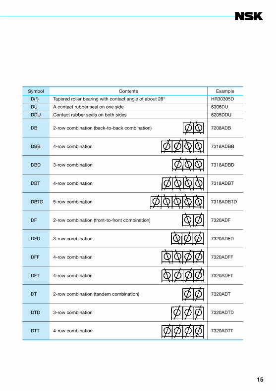
D(1) Tapered roller bearing with contact angle of about 28° HR30305D

DU A contact rubber seal on one side 6306DU

DDU Contact rubber seals on both sides 6205DDU

DB 2-row combination (back-to-back combination) 7208ADB

DBB 4-row combination 7318ADBB

DBD 3-row combination 7318ADBD

DBT 4-row combination 7318ADBT

DBTD 5-row combination 7318ADBTD

DF 2-row combination (front-to-front combination) 7320ADF

DFD 3-row combination 7320ADFD

DFF 4-row combination 7320ADFF

DFT 4-row combination 7320ADFT

DT 2-row combination (tandem combination) 7320ADT

DTD 3-row combination 7320ADTD

DTT 4-row combination 7320ADTT

16


Note ( 2 )（HR is added before bearing type symbol.


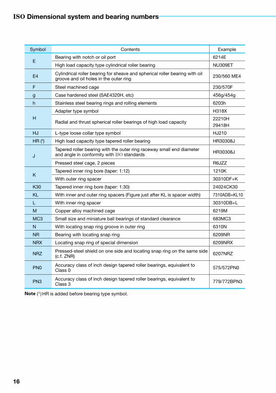
EBearing with notch or oil port 6214E

High load capacity type cylindrical roller bearing NU309ET

E4 Cylindrical roller bearing for sheave and spherical roller bearing with oilgroove and oil holes in the outer ring 230/560 ME4

F Steel machined cage 230/570F

g Case hardened steel (SAE4320H, etc) 456g/454g

h Stainless steel bearing rings and rolling elements 6203h

H

Adapter type symbol H318X

Radial and thrust spherical roller bearings of high load capacity22210H29418H

HJ L-type loose collar type symbol HJ210

HR (2) High load capacity type tapered roller bearing HR30308J

JTapered roller bearing with the outer ring raceway small end diameterand angle in conformity with ISO standards HR30308J

Pressed steel cage, 2 pieces R6JZZ

KTapered inner ring bore (taper: 1:12) 1210K

With outer ring spacer 30310DF+K

K30 Tapered inner ring bore (taper: 1:30) 24024CK30

KL With inner and outer ring spacers (Figure just after KL is spacer width) 7310ADB+KL10

L With inner ring spacer 30310DB+L

M Copper alloy machined cage 6219M

MC3 Small size and miniature ball bearings of standard clearance 683MC3

N With locating snap ring groove in outer ring 6310N

NR Bearing with locating snap ring 6209NR

NRX Locating snap ring of special dimension 6209NRX

NRZ Pressed-steel shield on one side and locating snap ring on the same side(c.f. ZNR) 6207NRZ

PN0 Accuracy class of inch design tapered roller bearings, equivalent toClass 0 575/572PN0

PN3 Accuracy class of inch design tapered roller bearings, equivalent toClass 3 779/772BPN3

16 17


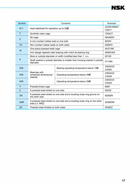
S11 Heat stabilized for operation up to 200°C22230CAMKE4C3S11

T Synthetic resin cage 7204CT

VNo cage NA4905V

A non-contact rubber seal on one side 6204V

VV Non-contact rubber seals on both sides 6306VV

WOne-piece pressed-steel cage NU210W

Inch design tapered roller bearing with notch at bearing ring 456W/454

X

Bore or outside diameter or width modified less than 1 mm 6310X

Shaft washer,s outside diameter is smaller than housing washer

,s outside

diameter 51130X

X26

Bearings withenhanced dimensionalstability

Bearing operating temperature below 150°C23032CDC3X26

X28 Operating temperature below 200°C23032CDC4X28

X29 Operating temperature below 250°C23032CDC4X29

Y Pressed-brass cage 608Y

Z A pressed-steel shield on one side 6203Z

ZN A pressed-steel shield on one side and a locating-snap-ring groove onthe other side 6208ZN

ZNR A pressed-steel shield on one side and a locating-snap-ring on the otherside (c.f. NRZ) 6208ZNR

ZZ Pressed-steel shields on both sides 6208ZZ

18

2. Dynamic load rating, fatigue life, and static load rating

2.1 Dynamic load rating

The basic dynamic load rating of rolling bearings is defined as the constant load applied on bearings with stationary outer rings that the inner rings can endure for a rating life (90% life) of one million revolutions. The basic load rating of radial bearings is defined as a central radial load of constant direction and magnitude, while the basic load rating of thrust bearings is defined as an axial load of constant magnitude in the same direction as the central axis.

This basic dynamic load rating is calculated by an equation shown in Table 1. The equation is based on the theory of G. Lundberg & A. Palmgren, and was adopted in ISO R281 : 1962 in 1962 and in JIS B 1518 : 1965 in Japan in March, 1965. Later on, these standards were established respectively as ISO 281 : 1990 and JIS B 1518 (under revision) after some modification.

The fatigue life of a bearing is calculated as follows:

L= 3

for a ball bearing ......................... (1)

L= 10/3

for a roller bearing .................... (2)

where, L: Rating fatigue life (106 rev) P: Dynamic equivalent load (N), {kgf} C: Basic dynamic load rating (N), {kgf}

The factor fc used in the calculation of Table 1 has a different value depending on the bearing type, as shown in Tables 2 and 3. The value fc of a radial ball bearing is the same as specified in JIS B 1518 : 1965, while that of a radial roller bearing was revised to be the maximum possible value. In this way, the factor fc determined from the processing accuracy and material has been at about the same level for the past 20 years.

During this period, however, bearings have undergone substantial improvement in terms of not only material, but also processing accuracy. As a result, the practical bearing life is extended considerably. It would be easier to use the above equations for calculations with improved bearings because the dynamic load rating already reflects the life extension factor. This concept of ISO 281 : 1990 and JIS B 1518 (under revision) has led to the increase of the basic dynamic load rating by multiplying by the rating factor bm. The value of the rating factor bm is as shown in Table 4.

( C )P

( C )P

18 19

Table 1 Calculation equation of basic dynamic load rating

Note ( 1 )　Diameter at the middle of the roller length Tapered roller: Arithmetic average value of roller large and small end diameters assuming the roller without chamfers Convex roller (asymmetric): Approximate value of roller diameter at the contact point of the roller and ribless raceway (generally outer ring raceway) without applying loadRemarks　When Dw>25.4 mm, Dw

1.8 becomes 3.647 Dw1.4

Classification Ball bearing Roller bearing

Radial bearing bm fc（i cos α）0.7 Z 2/3 Dw1.8 bm fc（i Lwe cos α）7/9 Z 3/4 Dwe

29/27

Single-rowthrust bearing

α 　90° bm fc Z 2/3 Dw1.8 bm fc Lwe

7/9 Z 3/4 Dwe29/27

α 　90° bm fc（cos α）0.7 tan α Z2/3 Dw1.8 bm fc（Lwe cos α）7/9 tan α Z 3/4 Dwe

29/27

Quantity symbols inequations

bm: Rating factor depending on normal material and manufacture qualityfc: Coefficient determined from shape, processing accuracy, and material of

bearing partsi: Number of rows of rolling elements in one bearingα : Nominal contact angle ( °)Z: Number of rolling elements per row

Dw: Diameter of ball (mm)Dwe: Diameter of roller used in calculation (1) (mm)Lwe: Effective length of roller (mm)

20

Dynamic load rating, fatigue life, and static load rating

Table 2 fc value of radial ball bearings

Note ( 1 )　Dpw is the pitch diameter of balls.Remarks　Figures in { } for kgf unit calculation

Dw cosα─────Dpw (1)

fc

Single-row deepgroove ball bearing,single/double rowangular contact ballbearing

Double-row deepgroove ball bearing

Self-aligning ballbearing

0.050.060.070.080.09

0.100.120.140.160.18

0.200.220.240.260.28

0.300.320.340.360.38

46.7 {4.76}49.1 {5.00}51.1 {5.21}52.8 {5.39}54.3 {5.54}

55.5 {5.66}57.5 {5.86}58.8 {6.00}59.6 {6.08}59.9 {6.11}

59.9 {6.11}59.6 {6.08}59.0 {6.02}58.2 {5.93}57.1 {5.83}

56.0 {5.70}54.6 {5.57}53.2 {5.42}51.7 {5.27}50.0 {5.10}

44.2 {4.51}46.5 {4.74}48.4 {4.94}50.0 {5.10}51.4 {5.24}

52.6 {5.37}54.5 {5.55}55.7 {5.68}56.5 {5.76}56.8 {5.79}

56.8 {5.79}56.5 {5.76}55.9 {5.70}55.1 {5.62}54.1 {5.52}

53.0 {5.40}51.8 {5.28}50.4 {5.14}48.9 {4.99}47.4 {4.84}

17.3 {1.76}18.6 {1.90}19.9 {2.03}21.1 {2.15}22.3 {2.27}

23.4 {2.39}25.6 {2.61}27.7 {2.82}29.7 {3.03}31.7 {3.23}

33.5 {3.42}35.2 {3.59}36.8 {3.75}38.2 {3.90}39.4 {4.02}

40.3 {4.11}40.9 {4.17}41.2 {4.20}41.3 {4.21}41.0 {4.18}

20 21

Table 3 fc value of radial roller　　　　　bearings

Dwecosα─────Dpw (2)

fc

0.010.020.030.040.05

0.060.070.080.090.10

0.120.140.160.180.20

0.220.240.260.280.30

52.1 {5.32}60.8 {6.20}66.5 {6.78}70.7 {7.21}74.1 {7.56}

76.9 {7.84}79.2 {8.08}81.2 {8.28}82.8 {8.45}84.2 {8.59}

86.4 {8.81}87.7 {8.95}88.5 {9.03}88.8 {9.06}88.7 {9.05}

77.2 {9.00}87.5 {8.92}86.4 {8.81}85.2 {8.69}83.8 {8.54}

Note ( 2 )　D

Remarks　

Dpw is the pitch diameter of rollers.

1. The fc value in the above table applies to a bearing in which the stress distribution in the length direction of roller is nearly uniform.2. Figures in { } for kgf unit calculation

Table 4 Value of rating factor bm

Bearing type bm

Radial Bearings

Deep groove ball bearingMagneto bearingAngular contact ball bearingBall bearing for rolling bearing unitSelf-aligning ball bearingSpherical roller bearingFilling slot ball bearingCylindrical roller bearingTapered roller bearingSolid needle roller bearing

1.31.31.31.31.31.151.11.11.11.1

Thrust Bearings

Thrust ball bearingThrust spherical roller bearingThrust tapered roller bearingThrust cylindrical roller bearingThrust needle roller bearing

1.31.151.111

22


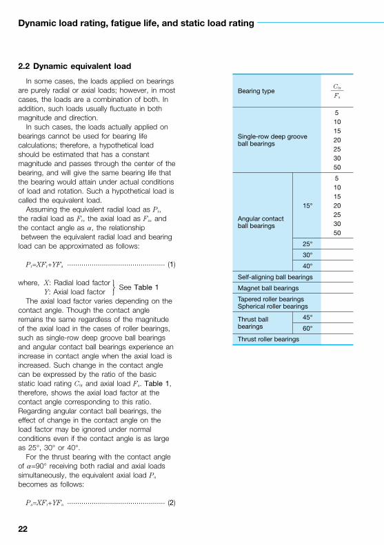
2.2 Dynamic equivalent load

In some cases, the loads applied on bearings are purely radial or axial loads; however, in most cases, the loads are a combination of both. In addition, such loads usually fluctuate in both magnitude and direction.

In such cases, the loads actually applied on bearings cannot be used for bearing life calculations; therefore, a hypothetical load should be estimated that has a constant magnitude and passes through the center of the bearing, and will give the same bearing life that the bearing would attain under actual conditions of load and rotation. Such a hypothetical load is called the equivalent load.

Assuming the equivalent radial load as Pr, the radial load as Fr, the axial load as Fa, and the contact angle as α, the relationship between the equivalent radial load and bearing load can be approximated as follows:

Pr=XFr+YFa ................................................ (1)

where, X: Radial load factor See Table 1 Y: Axial load factor

The axial load factor varies depending on the contact angle. Though the contact angle remains the same regardless of the magnitude of the axial load in the cases of roller bearings, such as single-row deep groove ball bearings and angular contact ball bearings experience an increase in contact angle when the axial load is increased. Such change in the contact angle can be expressed by the ratio of the basic static load rating C0r and axial load Fa. Table 1, therefore, shows the axial load factor at the contact angle corresponding to this ratio. Regarding angular contact ball bearings, the effect of change in the contact angle on the load factor may be ignored under normal conditions even if the contact angle is as large as 25°, 30° or 40°.

For the thrust bearing with the contact angle of α=90° receiving both radial and axial loads simultaneously, the equivalent axial load Pa becomes as follows:

Pa=XFr+YFa ................................................ (2)

Bearing typeC0r──Fa

Single-row deep grooveball bearings

　5101520253050

Angular contactball bearings

15°

　5101520253050

25° 　

30° 　

40° 　

Self-aligning ball bearings 　

Magnet ball bearings 　

Tapered roller bearingsSpherical roller bearings 　

Thrust ballbearings

45° 　

60° 　

Thrust roller bearings 　

22 23

Table 1 Value of factors X and Y

Single-row bearing Double-row bearing

eFa/Fr≦e Fa/Fr＞e Fa/Fr≦e Fa/Fr＞e

X Y X Y X Y X Y

1 0 0.56

1.261.491.641.761.851.922.13

　　　　

0.350.290.270.250.240.230.20

1 0 0.44

1.101.211.281.321.361.381.44

1

1.231.361.431.481.521.551.61

0.72

1.791.972.082.142.212.242.34

0.510.470.440.420.410.400.39

1 0 0.41 0.87 1 0.92 0.67 1.41 0.68

1 0 0.39 0.76 1 0.78 0.63 1.24 0.80

1 0 0.35 0.57 1 0.55 0.57 0.93 1.14

　　　　 1 0.42cot α 0.65 0.65cot α 1.5tan α1 0 0.5 2.5 　　　　 0.2

1 0 0.4 0.4cot α 1 0.45cot α 0.67 0.67cot α 1.5tan α

　　 0.66 1 1.18 0.59 0.66 1 1.25

　　 0.92 1 1.90 0.55 0.92 1 2.17

　　 tan α 1 1.5tan α 0.67 tan α 1 1.5tan α

Remarks 1.　Two similar single-row angular contact ball bearings are used. (1) DF or DB combination: Apply X and Y of double-row bearing. However, if obtain the axial load ratio of C0r/Fa, C0r should be half of C0r for the bearing set. (2) DT combination: Apply X and Y of single-row bearing. C0r should be half of C0r for the bearing set.2.　This table differs from JIS and ISO standards in the method of determining the axial load ratio C0r/Fa.

24


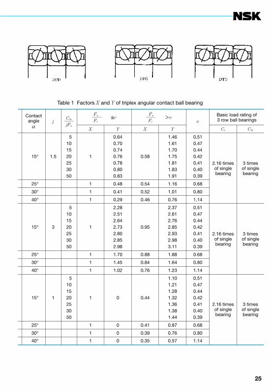
2.3 Dynamic equivalent load of triplex angular contact ball bearings

Three separate single-row bearings may be used side by side as shown in the figure when angular contact ball bearings are to be used to carry a large axial load. There are three patterns of combination, which are expressed by combination symbols of DBD, DFD, and DTD.

As in the case of single-row and double-row bearings, the dynamic equivalent load, which is determined from the radial and axial loads acting on a bearing, is used to calculate the fatigue life for these combined bearings.

Assuming the dynamic equivalent radial load as Pr, the radial load as Fr, and axial load as Fa, the relationship between the dynamic equivalent radial load and bearing load may be approximated as follows:

Pr=XFr+YFa ................................................ (1)where, X: Radial load factor See Table 1 Y: Axial load factor

The axial load factor varies with the contact angle. In an angular contact ball bearing, whose contact angle is small, the contact angle varies substantially when the axial load increases.

A change in the contact angle can be expressed by the ratio between the basic static load rating C0r and axial load Fa. Accordingly, for the angular contact ball bearing with a contact angle of 15°, the axial load factor at a contact angle corresponding to this ratio is shown. If the angular contact ball bearings have contact angles of 25°, 30° and 40°, the effect of change in the contact angle on the axial load factor may be ignored and thus the axial load factor is assumed as constant.

Arrangement Load direction

3 row matchedstack, axial loadis supported by2 rows.

3 row matchedstack, axial loadis supported by1 row.

3 row tandemmatched stack

SymbolDBD or

DFD( )

SymbolDBD or

DFD( )

SymbolDTD( )

24 25

Table 1 Factors X and Y of triplex angular contact ball bearing

Contactangleα

jC0r──jFa

　　　Fa──　　≦e　　　Fr

　　Fa──　　＞e　　　Fr e

Basic load rating of3 row ball bearings

X Y X Y Cr C0r

15° 1.5

5101520253050

1

0.640.700.740.760.780.800.83

0.58

1.461.611.701.751.811.831.91

0.510.470.440.420.410.400.39

2.16 timesof singlebearing

3 timesof singlebearing

25° 　　 1 0.48 0.54 1.16 0.68

30° 　　 1 0.41 0.52 1.01 0.80

40° 　　 1 0.29 0.46 0.76 1.14

15° 3

5101520253050

1

2.282.512.642.732.802.852.98

0.95

2.372.612.762.852.932.983.11

0.510.470.440.420.410.400.39



25° 　　 1 1.70 0.88 1.88 0.68

30° 　　 1 1.45 0.84 1.64 0.80

40° 　　 1 1.02 0.76 1.23 1.14

15° 1

5101520253050

1 0 0.44

1.101.211.281.321.361.381.44

0.510.470.440.420.410.400.39



25° 　　 1 0 0.41 0.87 0.68

30° 　　 1 0 0.39 0.76 0.80

40° 　　 1 0 0.35 0.57 1.14

26


2.4 Average of fluctuating load and speed

When the load applied on a bearing fluctuates, an average load which will yield the same bearing life as the fluctuating load should be calculated.(1) When the relation between load and rotating

speed can be partitioned into groups of rectangles (Fig. 1),

Load F1; Speed n1; Operating time t1

Load F2; Speed n2; Operating time t2 . . . . . . . . . Load Fn; Speed nn; Operating time tn

then the average load Fm may be calculated using the following equation:

Fm=p ................ (1)

where, Fm: Average of fluctuating load (N), {kgf}

p=3 for ball bearings p=10/3 for roller bearings

The average speed nm may be calculated as follows:

nm= .................... (2)

(2) When the load fluctuates almost linearly (Fig. 2), the average load may be calculated as follows:

　　　 Fm≒ (Fmin+2Fmax) .......................... (3)

where, Fmin: Minimum value of fluctuating load (N), {kgf}

Fmax: Maximum value of fluctuating load (N), {kgf}

(3) When the load fluctuation is similar to a sine wave (Fig. 3), an approximate value for the average load Fm may be calculated from the following equation:

In the case of Fig. 3 (a)Fm≒0.65 Fmax ........................................ (4)

In the case of Fig. 3 (b)Fm≒0.75 Fmax ........................................ (5)

F1pn1t1+F2

pn2t2 +...+ Fnpnntn

n1t1+n2t2 +......+ nntn

n1t1+n2t2+......+nntn

t1+t2+......+tn

13

26 27

Fig. 1　Incremental load variation Fig. 2　Simple load fluctuation

Fig. 3　Sinusoidal load variation

28


2.5 Combination of rotating and stationary loads

Generally, rotating, static, and indeterminate loads act on a rolling bearing. In certain cases, both the rotating load, which is caused by an unbalanced or a vibration weight, and the stationary load, which is caused by gravity or power transmission, may act simultaneously. The combined mean effective load when the indeterminate load caused by rotating and static loads can be calculated as follows. There are two kinds of combined loads; rotating and stationary which are classified depending on the magnitude of these loads, as shown in Fig. 1.

Namely, the combined load becomes a running load with its magnitude changing as shown in Fig. 1 (a) if the rotating load is larger than the static load. The combined load becomes an oscillating load with a magnitude changing as shown in Fig. 1 (b) if the rotating load is smaller than the stationary load.

In either case, the combined load F is expressed by the following equation:

F= FR2+FS

2–2FRFScos q ............................. (1)

where, FR: Rotating load (N), {kgf} FS: Stationary load (N), {kgf} q : Angle defined by rotating and

stationary loads

The value F can be approximated by Load Equations (2.1) and (2.2) which vary sinusoidally depending on the magnitude of FR and FS, that is, in such a manner that FR+FS becomes the maximum load Fmax and FR–FS becomes the minimum load Fmin for FR≫FS or FR≪FS.

FR≫FS, F=FR–FScos q .................................. (2.1)FR≪FS, F=FS–FRcos q .................................. (2.2)

The value F can also be approximated by Equations (3.1) and (3.2) when FR≒FS.FR>FS,

F=FR–FS+2FSsin ................................ (3.1)

FR>FS,

F=FS–FR+2FRsin ............................... (3.2)

Curves of Equations (1), (2.1), (3.1), and (3.2) are as shown in Fig. 2.

The mean value Fm of the load varying as expressed by Equations (2.1) and (2.2) or (3.1) and (3.2) can be expressed respectively by Equations (4.1) and (4.2) or (5.1) and (5.2).

Fm=Fmin +0.65 (Fmax–Fmin)FR≧FS, Fm=FR+0.3FS ................................ (4.1)FR≦FS, Fm=FS+0.3FR ................................ (4.2)

Fm=Fmin +0.75 (Fmax–Fmin)FR≧FS, Fm=FR+0.5FS ................................ (5.1)FR≦FS, Fm=FS+0.5FR ................................ (5.2)

Generally, as the value F exists somewhere among Equations (4.1), (4.2), (5.1), and (5.2), the factor 0.3 or 0.5 of the second terms of Equations (4.1) and (4.2) as well as (5.1) and (5.2) is assumed to change linearly along with FS /FR or FR /FS . Then, these factors may be expressed as follows:

0.3+0.2 , 0≦ ≦1

or 0.3+0.2 , 0≦ ≦1

Accordingly, Fm can be expressed by the following equation:

FR≧FS,

Fm=FR+(0.3+0.2 ) FS

=FR+0.3FS+0.2 ........................... (6.1)

FR≧FS,

Fm=FS+(0.3+0.2 ) FR

=FS+0.3FR+0.2 ........................... (6.2)

√————————————

q2

q2

FS

FR

FS

FR

FR

FS

FR

FS

FS

FR

FS2

FR

FR

FS

FR2

FS

28 29

Fig. 1　Combined load of rotating and stationary loads

Fig. 2　Chart of combined loads

30


2.6 Life calculation of multiple bearings as a group

When multiple rolling bearings are used in one machine, the fatigue life of individual bearings can be determined if the load acting on individual bearings is known. Generally, however, the machine becomes inoperative if a bearing in any part fails. It may therefore be necessary in certain cases to know the fatigue life of a group of bearings used in one machine.

The fatigue life of the bearings varies greatly and our fatigue life calculation equation

L= p

applies to the 90% life (also called

the rating fatigue life, which is either the gross number of revolution or hours to which 90% of multiple similar bearings operated under similar conditions can reach).

In other words, the calculated fatigue life for one bearing has a probability of 90%. Since the endurance probability of a group of multiple bearings for a certain period is a product of the endurance probability of individual bearings for the same period, the rating fatigue life of a group of multiple bearings is not determined solely from the shortest rating fatigue life among the individual bearings. In fact, the group life is much shorter than the life of the bearing with the shortest fatigue life.

Assuming the rating fatigue life of individual bearings as L1, L2, L3 ... and the rating fatigue life of the entire group of bearings as L, the below equation is obtained:

= + + + .................................... (1) where, e=1.1 (both for ball and roller bearings)

L of Equation (1) can be determined with ease by using Fig. 1.

Take the value L1 of Equation (1) on the L1 scale and the value of L2 on the L2 scale, connect them with a straight line, and read the intersection with the L scale. In this way, the value LA of

= +

is determined. Take this value LA on the L1 scale and the value L3 on the L2 scale, connect them with a straight line, and read an intersection with the L scale.In this way, the value L of

= + +

can be determined.

ExampleAssume that the calculated fatigue life of

bearings of automotive front wheels as follows:280 000 km for inner bearing320 000 km for outer bearingThen, the fatigue life of bearings of the wheel

can be determined at 160 000 km from Fig. 1.If the fatigue life of the bearing of the right-hand wheel takes this value, the fatigue life of the left-hand wheel will be the same. As a result, the fatigue life of the front wheels as a group will become 85 000 km.

( C )P

1Le

1L1

e

1L2

e

1L3

e

1LA

e

1L1

e

1L2

e

1Le

1L1

e

1L2

e

1L3

e

30 31

Fig. 1　Chart for life calculation

32


2.7 Load factor and fatigue life by machine

Loads acting on the bearing, rotating speed, and other conditions must be taken into account when selecting a bearing for a machine. Basic loads acting on a bearing are considered normally to include the weight of a rotating body supported by the bearing, load developed by power transmitted gears and belt, and other loads which can be estimated by calculation.Actually, in addition to the above loads, there are loads caused by unbalance of a rotating body, load developed due to vibration and shock during operation, etc., which are, however, difficult to determine accurately. In order to assume the dynamic equivalent load P necessary for selection of the bearing, therefore, the above basic load Fc is converted into a practical mean effective load by multiplying it by a certain factor. This factor is called the load factor fw, which is an empirical value. Table 1 shows the guideline of load factor fw for each machine and operating conditions. For example, when a part incorporating a bearing is subject to a radial load of Frc and an axial load of Fac, the dynamic equivalent load P can be expressed as follows, with load factors assumed respectively as fw1 and fw2:

P=Xfw1Frc+Yfw2Fac ....................................... (1)

Setting an unnecessarily long fatigue life during selection of a bearing is not economical because it will lead to a larger bearing. Moreover, the fatigue life of a bearing may not be the sole standard in certain cases in view of the strength, rigidity, and mounting dimensions of the shaft. In general, the bearing design life is set as a guideline for each machine and operation conditions to ensure selection of an adequate yet economical bearing.

Such a design life requires an empirical value called the fatigue life factor fh. Table 2 shows the fatigue life factors which are summarized for each machine and operating conditions. It is therefore necessary to determine the basic load rating C from the fatigue life factor fh appropriate to the bearing application purpose while using the equation as follows:

C≧ ...................................................... (2)

where, C: Basic dynamic load rating (N), {kgf} fn: Speed factor

The bearing must satisfy the calculated basic dynamic load rating C as shown above.

fh·Pfn

32 33

Table 2 Fatigue life factor fh for various bearing applications

Operatingperiods

Fatigue life factor fh and machine

　3 2 to 4 3 to 5 4 to 7 　6

Infrequently or onlyfor short periods

　Small motors for　home appli-　ances like　vacuum cleaners　Hand powered　tools

　Agricultural　equipment

Only occasionallybut reliability isimportant

　Motors for　home heaters　and air con-　ditioners　Construction　equipment

　Conveyors　Elevators

Intermittently forrelatively long periods

　Rolling mill　roll necks

　Small motors　Deck cranes　General cargo　cranes　Pinion stands　Passenger cars

　Factory motors　Machine tools　Transmissions　Vibrating　screens　Crushers

　Crane sheaves　Compressors　Specialized　transmissions

Intermittently formore than eighthours daily

　Escalators 　Centrifugal　separators　Air conditioning　equipment　Blowers　Woodworking　machines　Large motors　Axle boxes on　railway rolling　stock

　Mine hoists　Press fly-wheels　Railway traction　motors　Locomotive axle　boxes

　Papermaking　machines

Continuously andhigh reliability isimportant

　Waterworking　pumps　Electric power　station　Mine draining　pumps

Table 1 Value of load factor fw

Running conditions Typical machine fw

Smooth operation freefrom shock

Electric motors, machine tools,air conditioners 1 to 1.2

Normal operationAir blowers, compressors,elevators, cranes, paper makingmachines

1.2 to 1.5

Operation exposed toshock and vibration

Construction equipment, crushers,vibrating screens, rolling mills 1.5 to 3

34


2.8 Radial clearance and fatigue life

As shown in the catalog, etc., the fatigue life calculation equation of rolling bearings is Equation (1):

L= p

.................................................... (1)

where, L: Rating fatigue life (106rev) C: Basic dynamic load rating (N), {kgf} P: Dynamic equivalent load (N), {kgf} p: Index Ball bearing p=3,

Roller bearing p=

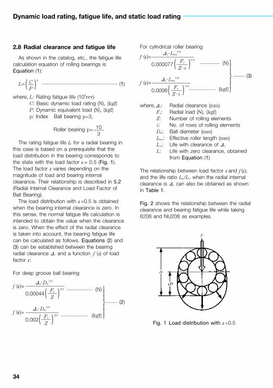
The rating fatigue life L for a radial bearing in this case is based on a prerequisite that the load distribution in the bearing corresponds to the state with the load factor ε = 0.5 (Fig. 1). The load factor ε varies depending on the magnitude of load and bearing internal clearance. Their relationship is described in 5.2 (Radial Internal Clearance and Load Factor of Ball Bearing).

The load distribution with ε =0.5 is obtained when the bearing internal clearance is zero. In this sense, the normal fatigue life calculation is intended to obtain the value when the clearance is zero. When the effect of the radial clearance is taken into account, the bearing fatigue life can be calculated as follows. Equations (2) and (3) can be established between the bearing radial clearance D r and a function f (ε) of load factor ε:

For deep groove ball bearing

f (ε)=

.................. (N)

........ (2)

f (ε)=

................... {kgf}

For cylindrical roller bearing

f (ε)=

.............. (N)

........ (3)f (ε)=

.................. {kgf}

where, D r: Radial clearance (mm) Fr: Radial load (N), {kgf} Z: Number of rolling elements i: No. of rows of rolling elements Dw: Ball diameter (mm) Lwe: Effective roller length (mm) L ε: Life with clearance of D r

L: Life with zero clearance, obtained from Equation (1)

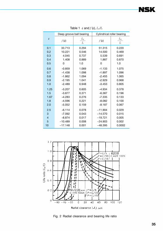
The relationship between load factor ε and f (ε), and the life ratio Lε/L, when the radial internal clearance is D r can also be obtained as shown in Table 1.

Fig. 2 shows the relationship between the radial clearance and bearing fatigue life while taking 6208 and NU208 as examples.

( C )P

103

D r·Dw1/3

( Fr )Z0.00044

2/3

D r·Dw1/3

( Fr )Z0.002

2/3

D r·Lwe0.8

( Fr )Z · i0.000077

0.9

D r·Lwe0.8

( Fr )Z · i0.0006

0.9

Fig. 1　Load distribution with ε=0.5

34 35

Table 1 ε and f (ε), Lε/L

εDeep groove ball bearing Cylindrical roller bearing

f (ε)Lε──L

f (ε)Lε──L

0.10.20.30.40.5

0.60.70.80.91.0

1.251.51.671.82.0

2.5345

10

33.71310.221

4.0451.4080

−　0.859−　1.438−　1.862−　2.195−　2.489

−　3.207−　3.877−　4.283−　4.596−　5.052

−　6.114−　7.092−　8.874

−10.489−17.148

0.2940.5460.7370.8891.0

1.0691.0981.0941.0410.948

0.6050.3710.2760.2210.159

0.0780.0430.0170.0080.001

51.31514.500

5.5391.8870

−　1.133−　1.897−　2.455−　2.929−　3.453

−　4.934−　6.387−　7.335−　8.082−　9.187

−11.904−14.570−19.721−24.903−48.395

0.2200.4690.6910.8701.0

1.0751.0961.0650.9680.805

0.3780.1960.1330.1000.067

0.0290.0150.0050.0020.0002

Fig. 2　Radial clearance and bearing life ratio

36


2.9 Misalignment of inner/outer rings and fatigue life of deep-groove ball bearings

A rolling bearing is manufactured with high accuracy, and it is essential to take utmost care with machining and assembly accuracies of surrounding shafts and housing if this accuracy is to be maintained. In practice, however, the machining accuracy of parts around the bearing is limited, and bearings are subject to misalignment of inner/outer rings caused by the shaft deflection under external load.

The allowable misalignment is generally 0.0006 ~ 0.003 rad (2’ to 10’) but this varies depending on the size of the deep-groove ball bearing, internal clearance during operation, and load.

This section introduces the relationship between the misalignment of inner/outer rings and fatigue life. Four different sizes of bearings are selected as examples from the 62 and 63 series deep-groove ball bearings.

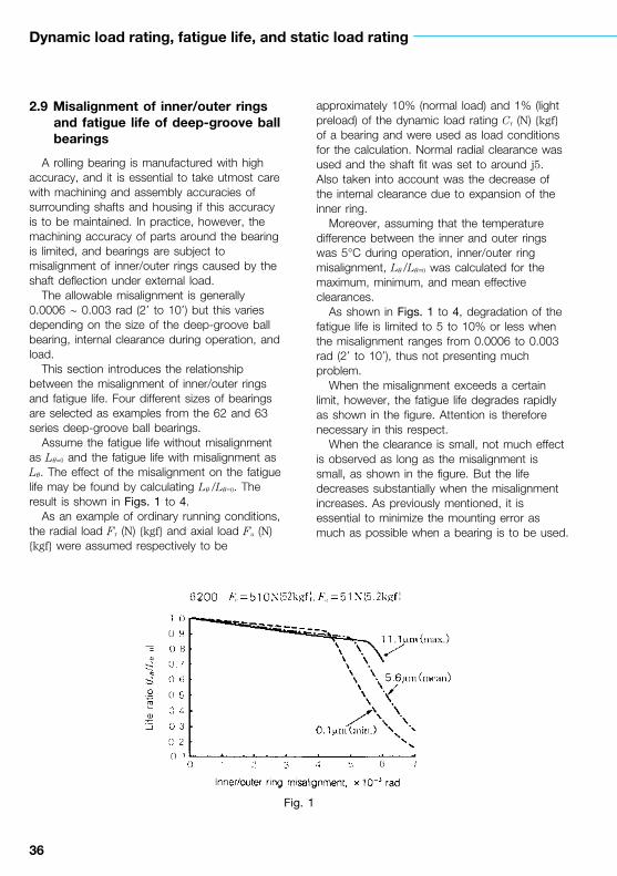
Assume the fatigue life without misalignment as Lq=0 and the fatigue life with misalignment as Lq. The effect of the misalignment on the fatigue life may be found by calculating Lq /Lq=0. The result is shown in Figs. 1 to 4.

As an example of ordinary running conditions, the radial load Fr (N) {kgf} and axial load Fa (N) {kgf} were assumed respectively to be

approximately 10% (normal load) and 1% (light preload) of the dynamic load rating Cr (N) {kgf} of a bearing and were used as load conditions for the calculation. Normal radial clearance was used and the shaft fit was set to around j5. Also taken into account was the decrease of the internal clearance due to expansion of the inner ring.

Moreover, assuming that the temperature difference between the inner and outer rings was 5°C during operation, inner/outer ring misalignment, Lq /Lq=0 was calculated for the maximum, minimum, and mean effective clearances.

As shown in Figs. 1 to 4, degradation of the fatigue life is limited to 5 to 10% or less when the misalignment ranges from 0.0006 to 0.003 rad (2’ to 10’), thus not presenting much problem.

When the misalignment exceeds a certain limit, however, the fatigue life degrades rapidly as shown in the figure. Attention is therefore necessary in this respect.

When the clearance is small, not much effect is observed as long as the misalignment is small, as shown in the figure. But the life decreases substantially when the misalignment increases. As previously mentioned, it is essential to minimize the mounting error as much as possible when a bearing is to be used.

Fig. 1

36 37

Fig. 2

Fig. 3

Fig. 4

38


2.10 Misalignment of inner/outer rings and fatigue life of cylindrical roller bearings

When a shaft supported by rolling bearings is deflected or there is some inaccuracy in a shoulder, there arises misalignment between the inner and outer rings of the bearings, thereby lowering their fatigue life. The degree of life degradation depends on the bearing type and interior design but also varies depending on the radial internal clearance and the magnitude of load during operation.

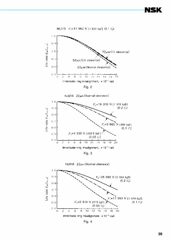
The relationship between the misalignment of inner/outer rings and fatigue life was determined, as shown in Figs. 1 to 4, while using cylindrical roller bearings NU215 and NU315 of standard design.

In these figures, the horizontal axis shows the misalignment of inner/outer rings (rad) while the vertical axis shows the fatigue life ratio Lq /Lq=0. The fatigue life without misalignment is Lq=0 and that with misalignment is Lq.

Figs. 1 and 2 show the case with constant load (10% of basic dynamic load rating Cr of a bearing) for each case when the internal clearance is a normal, C3 clearance, or C4 clearance. Figs. 3 and 4 show the case with constant clearance (normal clearance) when the load is 5%, 10%, and 20% of the basic dynamic load rating Cr.

Note that the median effective clearance in these examples was determined using m5/H7 fits and a temperature difference of 5°C between the inner and outer rings.

The fatigue life ratio for the clearance and load shows the same trend as in the case of other cylindrical roller bearings. But the life ratio itself differs among bearing series and dimensions, with life degradation rapid in 22 and 23 series bearings (wide type). It is advisable to use a bearing of special design when considerable misalignment is expected during application.

Fig. 1

38 39

Fig. 2

Fig. 3

Fig. 4

40


2.11 Fatigue life and reliability

Where any part failure may result in damage to the entire machine and repair of damage is impossible, as in applications such as aircraft, satellites, or rockets, greatly increased reliability is demanded of each component. This concept is being applied generally to durable consumer goods and may also be utilized to achieve effective preventive maintenance of machines and equipment.

The rating fatigue life of a rolling bearing is the gross number of revolutions or the gross rotating period when the rotating speed is constant for which 90% of a group of similar bearings running individually under similar conditions can rotate without suffering material damage due to rolling fatigue. In other words, fatigue life is normally defined at 90% reliability. There are other ways to describe the life. For example, the average value is employed frequently to describe the life span of human beings. However, if the average value were used for bearings, then too many bearings would fail before the average life value is reached. On the other hand, if a low or minimum value is used as a criterion, then too many bearings would have a life much longer than the set value. In this view, the value 90% was chosen for common practice. The value 95% could have been taken as the statistical reliability, but nevertheless, the slightly looser reliability of 90% was taken for bearings empirically from the practical and economical viewpoint. A 90% reliability however is not acceptable for parts of aircraft or electronic computers or communication systems these days, and a 99% or 99.9% reliability is demanded in some of these cases.

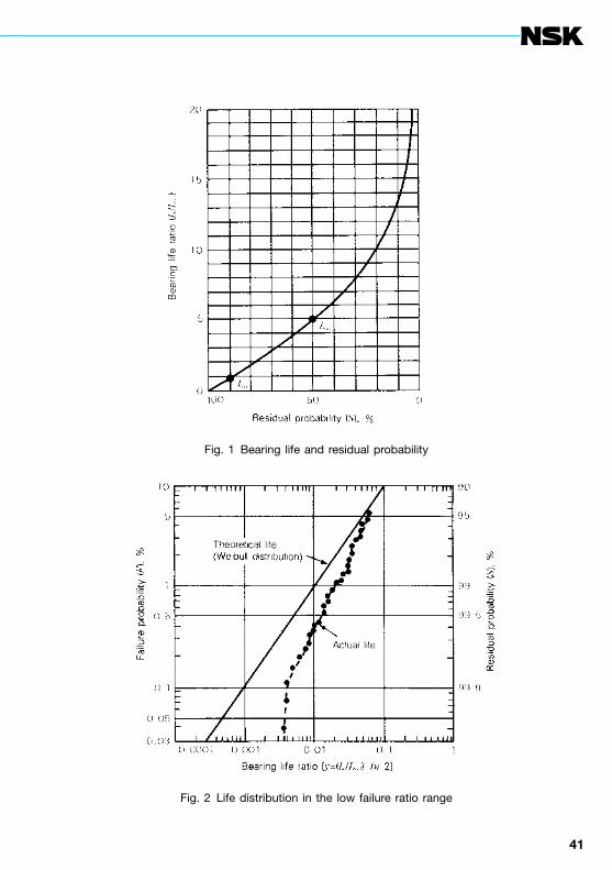
The fatigue life distribution when a group of similar bearings are operated individually under similar conditions is shown in Fig. 1. The Weibull equation can be used to describe the fatigue life distribution within a damage ratio of 10 to 60% (residual probability of 90 to 40%).

Below the damage ratio of 10% (residual probability of 90% or more), however, the rolling fatigue life becomes longer than the theoretical curve of the Weibull distribution, as shown in Fig. 2. This is a conclusion drawn from the life test of numerous, widely-varying bearings and an analysis of the data.

When bearing life with a failure ratio of 10% or less (for example, the 95% life or 98% life) is to be considered on the basis of the above concept, the reliability factor a1 as shown in the table below is used to check the life. Assume here that the 98% life L2 is to be calculated for a bearing whose rating fatigue life L10 was calculated at 10 000 hours. The life can be calculated as L2=0.33´L10=3 300 hours. In this manner, the reliability of the bearing life can be matched to the degree of reliability required of the equipment and difficulty of overhaul and inspection.

Apart from rolling fatigue, factors such as lubrication, wear, sound, and accuracy govern the durability of a bearing. These factors must be taken into account, but the endurance limit of these factors varies depending on application and conditions.

Table 1 Reliability factor

Reliability, % 90 95 96 97 98 99

Life, LaL10

rating life L5 L4 L3 L2 L1

Reliability factor, a1

1 0.62 0.53 0.44 0.33 0.21

40 41

Fig. 1　Bearing life and residual probability

Fig. 2　Life distribution in the low failure ratio range

42


2.12 Oil film parameters and rolling fatigue life

Based on numerous experiments and experiences, the rolling fatigue life of rolling bearings can be shown to be closely related to the lubrication.

The rolling fatigue life is expressed by the maximum number of rotations, which a bearing can endure, until the raceway or rolling surface of a bearing develops fatigue in the material, resulting in flaking of the surface, under action of cyclic stress by the bearing. Such flaking begins with either microscopic non-uniform portions (such as non-metallic inclusions, cavities) in the material or with microscopic defect in the material’s surface (such as extremely small cracks or surface damage or dents caused by contact between extremely small projections in the raceway or rolling surface). The former flaking is called sub-surface originating flaking while the latter is surface-originating flaking.

The oil film parameter (L), which is the ratio between the resultant oil film thickness and surface roughness, expresses whether or not the lubrication state of the rolling contact surface is satisfactory. The effect of the oil film grows with increasing L. Namely, when L is large (around 3 in general), surface-originating flaking due to contact between extremely small projections in the surface is less likely to occur. If the surface is free from defects (flaw, dent, etc.), the life is determined mainly by sub-surface originating flaking. On the other hand, a decrease in L tends to develop surface-originating flaking, resulting in degradation of the bearing’s life. This state is shown in Fig. 1.

NSK has performed life experiments with about 370 bearings within the range of L=0.3 ~ 3 using different lubricants and bearing materials (● and ▲ in Fig. 2). Fig. 2 shows a summary of the principal experiments selected from among those reported up to now. As is evident, the life decreases rapidly at around L≒1 when compared with the life values at around L=3 ~ 4 where life changes at a slower rate. The life becomes about 1/10 or less at L≦0.5. This is a result of severe surface-originating flaking.

Accordingly, it is advisable for extension of the fatigue life of rolling bearings to increase the oil film parameter (ideally to a value above 3) by improving lubrication conditions.

42 43

Fig. 1　Expression of life according to L (Tallian, et al.)

Fig. 2　Typical experiment with L and rolling fatigue life (Expressed with reference to the life at L =3)

44


2.13 EHL oil film parameter calculation diagram

Lubrication of rolling bearings can be expressed by the theory of elastohydrodynamic lubrication (EHL). Introduced below is a method to determine the oil film parameter (oil film ─ surface roughness ratio), the most critical among the EHL qualities.

2.13.1 Oil film parameterThe raceway surfaces and rolling surfaces of

a bearing are extremely smooth, but have fine irregularities when viewed through a microscope. As the EHL oil film thickness is in the same order as the surface roughness, lubricating conditions cannot be discussed without considering this surface roughness. For example, given a particular mean oil film thickness, there are two conditions which may occur depending on the surface roughness. One consists of complete separation of the two surfaces by means of the oil film (Fig. 1 (a)). The other consists of metal contact between surface projections (Fig. 1 (b)). The degradation of lubrication and surface damage is attributed to case (b). The symbol lambda (L) represents the ratio between the oil film thickness and roughness. It is widely employed as an oil film parameter in the study and application of EHL.

L=h/s ........................................................ (1)

where h: EHL oil film thickness s: Combined roughness ( s1

2+s22 )

s1, s2: Root mean square (rms) roughness of each contacting surface

The oil film parameter may be correlated to the formation of the oil film as shown in Figs. 2 and the degree of lubrication can be divided into three zones as shown in the figure.

2.13.2 Oil film parameter calculation diagram

The Dowson-Higginson minimum oil film thickness equation shown below is used for the diagram:

Hmin=2.65 ................................... (2)

The oil film thickness to be used is that of the inner ring under the maximum rolling element load (at which the thickness becomes minimum).

Equation (2) can be expressed as follows by grouping into terms (R) for speed, (A) for viscosity, (F ) for load, and (J ) for bearing technical specifications. t is a constant.

L=t ·R·A·F ·J ............................................ (3)

R and A may be quantities not dependent on a bearing. When the load P is assumed to be between 98 N {10 kgf} and 98 kN {10 tf}, F changes by 2.54 times as F∝ P –0.13. Since the actual load is determined roughly from the bearing size, however, such change may be limited to 20 to 30%. As a result, F is handled as a lump with the term J of bearing specifications [F=F (J )]. Traditional Equation (3) can therefore be grouped as shown below:

L=T·R ·A ·D .............................................. (4)

where, T: Factor determined by the bearing Type

R: Factor related to Rotation speed A: Factor related to viscosity (viscosity

grade α: Alpha) D: Factor related to bearing Dimensions

√————

G0.54U 0.7

W 0.13

44 45

h

h

100

80

60

40

20

00.4 0.6 2 4 6 101

(a) Good roughness

(b) High roughness

Surface damage range

Surface damage range whensliding is large

(Short life)Long-life range

Normal bearingoperating conditions

Oil film parameter （）

Oil

film

form

ing

rat

e, %

Λ

Fig. 1　Oil film and surface roughness

Fig. 2　Effect of oil film on bearing performance

46


The oil film parameter L, which is most vital among quantities related to EHL, is expressed by a simplified equation shown below. The fatigue life of rolling bearings becomes shorter when L is smaller.

In the equation L=T·R ·A ·D terms include A for oil viscosity h0 (mPa ·s, {cp}), R for the speed n (min–1), and D for bearing bore diameter d (mm). The calculation procedure is described below.

(1) Determine the value T from the bearing type (Table 1).

(2) Determine the R value for n (min–1) from Fig. 3.

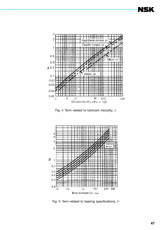
(3) Determine A from the absolute viscosity (mPa ·s, {cp}) and oil kind in Fig. 4. Generally, the kinematic viscosity ν0 (mm2/s, {cSt}) is used and conversion is made as follows:

h0=r ·ν0 ...................................................... (5)

r is the density (g/cm3) and uses the approximate value as shown below:

Mineral oil r=0.85Silicon oil r=1.0Diester oil r=0.9

When it is not known whether the mineral oil is naphthene or paraffin, use the paraffin curve shown in Fig. 4.

(4) Determine the D value from the diameter series and bore diameter d (mm) in Fig. 5.

(5) The product of the above values is used as an oil film parameter.

Table 1 Value T

Bearing type Value T

Ball bearingCylindrical roller bearingTapered roller bearingSpherical roller bearing

1.51.01.10.8

Fig. 3　Speed term, R

46 47

Fig. 4　Term related to lubricant viscosity, A

Fig. 5　Term related to bearing specifications, D

48


Examples of EHL oil film parameter calculation are described below.(Example 1)The oil film parameter is determined when a deep groove ball bearing 6312 is operated with paraffin mineral oil (h0=30 mPa ·s, {cp}) at the speed n =1 000 min–1.

(Solution)d=60 mm and D=130 mm from the bearing catalog.T=1.5 from Table 1R=3.0 from Fig. 3A=0.31 from Fig. 4D=1.76 from Fig. 5Accordingly, L=2.5

(Example 2)The oil film parameter is determined when a cylindrical roller bearing NU240 is operated with paraffin mineral oil (h0=10 mPa ·s, {cp}) at the speed n=2 500 min–1.

(Solution)d=200 mm and D=360 mm from the bearing catalog.T=1.0 from Table 1R=5.7 from Fig. 3A=0.13 from Fig. 4D=4.8 from Fig. 5Accordingly, L=3.6

2.13.3 Effect of oil shortage and shearing　　　heat generation

The oil film parameter obtained above is the value when the requirements, that is, the contact inlet fully flooded with oil and isothermal inlet are satisfied. However, these conditions may not be satisfied depending on lubrication and operating conditions.

One such condition is called starvation, and the actual oil film paramerer value may become smaller than determined by Equation (4). Starvation might occur if lubrication becomes limited. In this condition, a guideline for adjusting the oil film parameter is 50 to 70% of the value obtained from Equation (4).

Another effect is the localized temperature rise of oil in the contact inlet due to heavy shearing during high-speed operation, resulting in a decrease of the oil viscosity. In this case, the oil film parameter becomes smaller than the isothermal theoretical value. The effect of shearing heat generation was analyzed by Murch and Wilson, who established the decrease factor of the oil film parameter. An approximation using the viscosity and speed (pitch diameter of rolling element set Dpw ´ rotating speed per minute n as parameters) is shown in Fig. 6. By multiplying the oil film parameter determined in the previous section by this decrease factor Hi the oil film parameter considering the shearing heat generation is obtained.Nameny;

L=Hi ·T ·R ·A ·D ......................................... (6)

Note that the average of the bore and outside diameters of the bearings may be used as the pitch diameter Dpw (dm) of rolling element set.

Conditions for the calculation (Example 1) include dmn=9.5 ´ 104 and h0=30 mPa ·s, {cp}, and Hi is nearly equivalent to 1 as is evident from Fig. 6. There is therefore almost no effect of shearing heat generation. Conditions for (Example 2) are dmn=7´105 and h0=10 mPa ·s, {cp} while Hi=0.76, which means that the oil film parameter is smaller by about 25%. Accordingly, L is actually 2.7, not 3.6.

48 49

Fig. 6　Oil film thickness decrease factor Hi due to shearing heat generation

50


2.14 Fatigue analysis

It is necessary for prediction of the fatigue life of rolling bearings and estimation of the residual life to know all fatigue break-down phenomena of bearings. But, it will take some time before we reach a stage enabling prediction and estimation. Rolling fatigue, however, is fatigue proceeding under compressive stress at the contact point and known to develop extremely great material change until breakdown occurs. In many cases, it is possible to estimate the degree of fatigue of bearings by detecting material change. However, this estimation method is not effective in the cases where the defects in the raceway surface cause premature cracking or chemical corrosion occurs on the raceway. In these two cases, flaking grows in advance of the material change.

2.14.1 Measurement of fatigue degreeThe progress of fatigue in a bearing can be

determined by using an X-ray to measure changes in the residual stress, diffraction half-value width, and retained austenite amount.

These values change as the fatigue progresses as shown in Fig. 1. Residual stress, which grows early and approaches the saturation value, can be used to detect extremely small fatigue. For large fatigue, change of the diffraction half-value width and retained austenite amount may be correlated to the progress of fatigue. These measurements with X-ray are put together into one parameter (fatigue index) to determine the relationship with the endurance test period of a bearing.

Measured values were collected by carrying out endurance test with many ball, tapered roller, and cylindrical roller bearings under various load and lubrication conditions. Simultaneously, measurements were made on bearings used in actual machines.

Fig. 2 summarizes the data. Variance is considerable because data reflects the complexity of the fatigue phenomenon. But, there exists correlation between the fatigue index and the endurance test period or operating hours. If some uncertainty is allowed, the fatigue degree can be handled quantitatively.

Description of “sub-surface fatigue” in Fig. 2 applies to the case when fatigue is governed by internal shearing stress. “Surface fatigue” shows correlation when the surface fatigue occurs earlier and more severely than sub-surface fatigue due to contamination or oil film breakdown of lubricating oil.

50 51

Fig. 1　Change in X-ray measurements

Fig. 2　Fatigue progress and fatigue index

52


2.14.2 Surface and sub-surface fatiguesRolling bearings have an extremely smooth

finish surface and enjoy relatively satisfactory lubrication conditions. It has been considered that internal shearing stress below the rolling surface governs the failure of a bearing.

Shearing stress caused by rolling contact becomes maximum at a certain depth below the surface, with a crack (which is an origin of break-down) occurring initially under the surface. When the raceway is broken due to such sub-surface fatigue, the fatigue index as measured in the depth direction is known to increase according to the theoretical calculation of shearing stress, as is evident from an example of the ball bearing shown in Fig. 3.

The fatigue pattern shown in Fig. 3 occurs mostly when lubrication conditions are satisfactory and oil film of sufficient thickness is formed in rolling contact points. The basic dynamic load rating described in the bearing catalog is determined using data of bearing failures according to the above internal fatigue pattern.

Fig. 4 shows an example of a cylindrical roller bearing subject to endurance test under lubrication conditions causing unsatisfactory oil film. It is evident that the surface fatigue degree rises much earlier than the calculated life.

In this test, all bearings failed before sub-surface fatigue became apparent. In this way, bearing failure due to surface fatigue is mostly attributed to lubrication conditions such as insufficient oil film due to excessively low oil viscosity or entry of foreign matters or moisture into lubricant.

Needless to say, bearing failure induced by surface fatigue occurs in advance of that by sub-surface fatigue. Bearings in many machines are exposed frequently to danger of initiating such surface fatigue and, in most of the cases, failure by surface fatigue prior to failure due to sub-surface fatigue (which is the original life limit of bearings).

Fatigue analysis of bearings used in actual machines shows not the sub-surface fatigue pattern, but the surface fatigue pattern as shown in the figure in overwhelmingly high percentage.

In this manner, knowing the distribution of the fatigue index in actually used bearings leads to an understanding of effective information not only on residual life of bearings, but also on lubrication and load conditions.

52 53

Fig. 3　Progress of sub-surface fatigue

Fig. 4　Progress of surface fatigue

54


2.14.3 Analysis of practical bearing (1)Bearings for automotive transmissions must

overcome difficult problems of size and weight reduction as well as extension of durable life to meet the ever increasing efforts to conserve energy.

Fig. 5 shows an example of fatigue analysis of bearings used in the transmission of an actual passenger car. Analysis of the transmission bearings of various vehicles reveals the surface fatigue pattern as shown in Fig. 5, but almost no progress of sub-surface fatigue which is used as a criterion for calculating the bearing life.

In other words, these bearings develop less fatigue under external bearing loads but they eventually suffer damage due to fatigue by surface force on the rolling surface though they can be used for a long time.

This may be attributable to indentations caused by inclusions of extremely small foreign matters from the gear oil, which in turn cause excessive fatigue of the surface.

As is evident from Fig. 5, the fatigue index is heaviest in the counter front bearing where the load is most severe, followed by the counter rear bearing where the load is lightest. This surprising fact may be due to the fact that the counter shaft bearings are immersed in gear oil which often has many foreign particles suspend in it. Thus, metal chips in the gear oil eventually contact and abrade the counter shaft bearings.

Fig. 6 shows the result of the durability test and fatigue analysis data with two kinds of bearings used in a transmission of an actual vehicle.

As is known from above the analytical result, a bearing with a special seal (sealed clean bearing), which prevents entry of foreign matter in gear oil while allowing entry of oil only, offers remarkably extended life. In this way, the life is extended by more than ten times when compared with an open type bearing without a seal.

The fatigue pattern shows change in the sub-surface fatigue pattern in the sealed clean bearing, indicating that reduction of surface fatigue contributes greatly to the remarkable life extension.

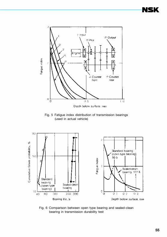
54 55

Fig. 5　Fatigue index distribution of transmission bearings (used in actual vehicle)

Fig. 6　Comparison between open type bearing and sealed-clean bearing in transmission durability test

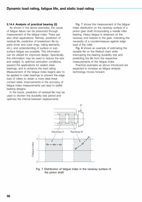
56


2.14.4 Analysis of practical bearing (2)As shown in the above examples, the cause

of fatigue failure can be presumed through measurement of the fatigue index. There are also other applications. Namely, prediction of residual life, prediction of breakdown life by parts (inner and outer rings, rolling elements, etc.), and understanding of surface or sub-surface fatigue are possible. This information can be utilized for improved design. Specifically, this information may be used to reduce the size and weight, to optimize lubrication conditions, expand the applications for sealed clean bearings, and to enhance the load rating. Measurement of the fatigue index begins also to be applied in roller bearings to prevent the edge load of rollers to obtain a more ideal linear contact state. Improvements in the accuracy of fatigue index measurements can lead to better bearing designs.

In the future, prediction of residual life may be used to shorten the durability test period and optimize the interval between replacements.

Fig. 7 shows the measurement of the fatigue index distribution on the raceway surface of a pinion gear shaft incorporating a needle roller bearing. Heavy fatigue is observed on the raceway end nearest to the gear, indicating the necessity of a countermeasure against edge load of the roller.

Fig. 8 shows an example of estimating the durable life on the Weibull chart while interrupting the bearing durability test and predicting the life from the respective measurements of the fatigue index.

Practical examples as above introduced are expected to increase as fatigue analysis technology moves forward.

P

2

1

0

Raceway BRaceway A

Fatig

ue in

dex

Fig. 7　Distribution of fatigue index in the raceway surface of the pinion shaft

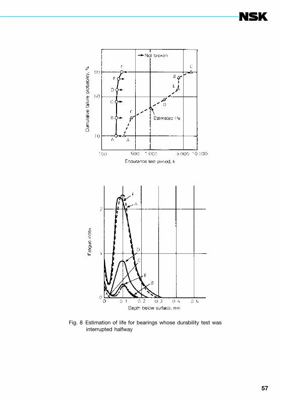
56 57

Fig. 8　Estimation of life for bearings whose durability test was interrupted halfway

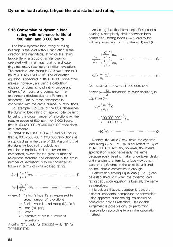
58


2.15 Conversion of dynamic load rating with reference to life at 500 min–1 and 3 000 hours

The basic dynamic load rating of rolling bearings is the load without fluctuation in the direction and magnitude, at which the rating fatigue life of a group of similar bearings operated with inner rings rotating and outer rings stationary reaches one million revolutions. The standard load rating is 33.3 min–1 and 500 hours (33.3´500´60=106). The calculation equation is specified in JIS B 1518. Some other makers, however, are using a calculation equation of dynamic load rating unique and different from ours, and comparison may encounter difficulties due to difference in standards. One of these differences is concerned with the gross number of revolutions.

For example, TIMKEN of the USA determines the dynamic load rating of tapered roller bearing by using the gross number of revolutions for the rotating speed of 500 min–1 for 3 000 hours, that is, 500´3 000´60=90 000 000 revolutions, as a standard. TORRINGTON uses 33.3 min–1 and 500 hours, that is, 33.3´500´60=1 000 000 revolutions as a standard as in the case of JIS. Assuming that the dynamic load rating calculation equation is basically similar between both companies, except for the gross number of revolutions standard, the difference in the gross number of revolutions may be converted as follows in terms of dynamic load rating:

LT= p

ńT ........................................... (1)

LR= p

ńR ........................................... (2)

where, L: Rating fatigue life as expressed by gross number of revolutions

C: Basic dynamic load rating (N), {kgf} P: Load (N), {kgf} p: Power n: Standard of gross number of

revolutionsA suffix “T” stands for TIMKEN while “R” for TORRINGTON.

Assuming that the internal specification of a bearing is completely similar between both companies, setting loads PT=PR lead to the following equation from Equations (1) and (2):

p

ńT

= =1 ................................. (3)p

ńR

CR

p= CT

p ................................................ (4)

Set nT=90 000 000, nR=1 000 000, and

power p= (applicable to roller bearings) in

Equation (4):

CR= CT

　= CT

　=90 CT ................................................ (5)

Namely, the value 3.857 times the dynamic load rating CT of TIMKEN is equivalent to CR of TORRINGTON. Actually, however, the internal specification is not necessarily the same because every bearing maker undertakes design and manufacture from its unique viewpoint. In case of a difference in the units (SI unit and pound), simple conversion is enough.

Relationship among Equations (3) to (5) can be established only when the dynamic load rating calculation equation is basically the same as described.If it is evident that the equation is based on different standards, comparison or conversion using apparent numerical figures should be considered only as reference. Reasonable judgement is possible only by performing recalculation according to a similar calculation method.

( CT )PT

( CR )PR

( CT )PT

( CR )PR

LT

LR

nT

nR

103

( nT )nR

1p

( 90 000 000 )1 000 000

310

310

60


2.16 Basic static load ratings and static equivalent loads

(1) Basic static load ratingWhen subjected to an excessive load or a

strong shock load, rolling bearings undergo a local permanent deformation of the rolling elements and raceway surface if the elastic limit is exceeded. The nonelastic deformation increases in both area and depth as the load increases, and when the load exceeds a certain limit, the smooth running of the bearing is impeded.

The basic static load rating is defined as that static load which produces the following calculated contact stress at the center of the contact area between the rolling element subjected to the maximum stress and the raceway surface.

For self-aligning ball bearings4 600 MPa {469 kgf/mm2}

For other ball bearings4 200 MPa {428 kgf/mm2}

For roller bearings4 000 MPa {408 kgf/mm2}

In this most heavily stressed contact area, the sum of the permanent deformation of the rolling element and that of the raceway is nearly 0.0001 times the rolling element’s diameter. The basic static load rating C0 is written C0r for radial bearings and C0a for thrust bearings in the bearing tables.

In addition, following the modification of the criteria for the basic static load rating by ISO, the new C0 values for NSK’s ball bearings became about 0.8 to 1.3 times the past values and those for roller bearings about 1.5 to 1.9 times. Consequently, the values of permissible static load factor fs have also changed, so please pay attention to this.

In the above description, the static load rating is not the load for failure (crack) of rolling element and bearing ring. Since the load necessary to crush a rolling element is more than seven times the static load rating, this is a sufficient safety factor against failure load when considering general machine equipment.

(2) Static equivalent loadThe static equivalent load must be considered

for radial bearings exposed to synthetic loads or axial loads only and for thrust bearings exposed to axial loads and slight radial loads.

The static equivalent load is a hypothetical load of a magnitude causing a contact stress (equivalent to the maximum contact stress occurring under actual load conditions) in the contact between the rolling element and raceway under maximum load when the bearing is stationary (including extremely low speed rotation and low-speed oscillation). This equivalent load is the radial load acting through a bearing center for radial bearings and the axial load in a direction aligned to the central axis in the case of thrust bearings.(a) Static equivalent load of radial bearingsThe static equivalent load of radial bearings is taken as the larger value of the two values obtained from the two equations below:

P0=XFr+Y0 Fa .............................................. (1)

P0=Fr .......................................................... (2)

where, P0: Static equivalent load (N), {kgf} Fr: Radial load (N), {kgf} Fa: Axial load (N), {kgf} X0: Static radial load factor Y0: Static axial load factor(b) Static equivalent load of thrust bearings

P0=X0 Fr+Fa α≠90° ................................... (3)

where, P0: Static equivalent load (N), {kgf} α : Nominal contact angleNote that the accuracy of this equation decreases when Fa<X0 Fr.Values X0 and Y0 of Equations (1) and (3) are as shown in Table 2.Note that P0=Fa for a thrust bearing with α=90°

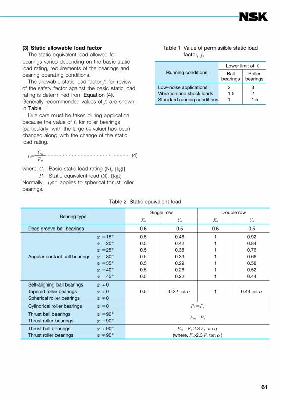
60 61

(3) Static allowable load factorThe static equivalent load allowed for

bearings varies depending on the basic static load rating, requirements of the bearings and bearing operating conditions.

The allowable static load factor fs for review of the safety factor against the basic static load rating is determined from Equation (4). Generally recommended values of fs are shown in Table 1.

Due care must be taken during application because the value of fs for roller bearings (particularly, with the large C0 value) has been changed along with the change of the static load rating.

fs= ....................................................... (4)

where, C0: Basic static load rating (N), {kgf} P0: Static equivalent load (N), {kgf}Normally, fs≧4 applies to spherical thrust roller bearings.

C0

P0

Table 1 Value of permissible static load factor, fs

Running conditionsLower limit of fs

Ballbearings

Rollerbearings

Low-noise applicationsVibration and shock loadsStandard running conditions

21.51

321.5

Table 2 Static epuivalent load

Bearing typeSingle row Double row

X0 Y0 X0 Y0

Deep groove ball bearings 0.6 0.5 0.6 0.5

Angular contact ball bearings

α ＝15°α ＝20°α ＝25°α ＝30°α ＝35°α ＝40°α ＝45°

0.50.50.50.50.50.50.5

0.460.420.380.330.290.260.22

1111111

0.920.840.760.660.580.520.44

Self-aligning ball bearingsTapered roller bearingsSpherical roller bearings

α ≠0α ≠0α ≠0

0.5 0.22 cot α 1 0.44 cot α

Cylindrical roller bearings α ＝0 P0＝Fr

Thrust ball bearingsThrust roller bearings

α ＝90°α ＝90°

P0a＝Fa

Thrust ball bearingsThrust roller bearings

α ≠90°α ≠90°

P0a＝Fa　2.3 Fr tan α(where, Fa>2.3 Fr tan α )

62

3. Bearing fitting practice

3.1 Load classifications

Bearing loads can be classified in various ways. With respect to magnitude, loads are classified as light, medium, or heavy; with respect to time, they are called stationary, fluctuating, or shock; and with respect to direction, they are divided into rotating (or “circumferential”), stationary (or “spot”), or indeterminate. The terms, “rotating”, “static”, and “indeterminate”, do not apply to the bearing itself, but instead are used to describe the load acting on each of the bearing rings.

Whether an interference fit or a loose fit should be adopted depends on whether the load applied to the inner and outer rings is rotating or stationary. A so-called “rotating load” is one where the loading direction on a bearing ring changes continuously regardless of whether the bearing ring itself rotates or remains stationary. On the other hand, a so called “stationary load” is one where the loading direction on a bearing ring is the same regardless of whether the bearing ring itself rotates or remains stationary.

As an example, when the load direction on a bearing remains constant and the inner ring rotates and the outer ring stays fixed, a rotating load is applied to the inner ring and a stationary load to the outer ring. In the case that the majority of the bearing load is an unbalanced load due to rotation, even if the inner ring rotates and the outer ring stays fixed, a stationary load is applied to the inner ring and a rotating load to the outer ring. (See Table 1).

Depending on the actual conditions, the situation is not usually as simple as described above. The loads may vary in complex ways with the load direction being a combination of fixed and rotating loads caused by mass, by imbalance, by vibration, and by power transmission. If the load direction on a bearing ring is highly irregular or a rotating load and stationary load are applied alternatively, such a load is called an indeterminate load.

The fit of a bearing ring on which a rotating load is applied should generally be an interference fit. If a bearing ring, on which a rotating load is applied, is mounted with a loose

fit, the bearing ring may slip on the shaft or in the housing and, if the load is heavy, the fitting surface may be damaged or fretting corrosion may occur. The tightness of the fit should be sufficient to prevent the interference from becoming zero as a result of the applied load and a temperature difference between the inner ring and shaft or between the outer ring and housing during operation. Depending on the operation conditions, the inner ring fitting is usually k5, m5, n6, etc. and for the outer ring, it is N7, P7, etc.

For large bearings, to avoid the difficulty of mounting and dismounting, sometimes a loose fit is adopted for the bearing ring on which a rotating load is applied. In such a case, the shaft material must be sufficiently hard, its surface must be well finished, and a lubricant needs to be applied to minimize damage due to slipping.

There is no problem with slipping between the shaft or housing for a bearing ring on which a stationary load is applied; therefore, a loose fit or transition fit can be used. The looseness of the fit depends on the accuracy required in use and the reduction in the load distribution range caused by bearing-ring deformation. For inner rings, g6, h6, js5( j5), etc. are often used, and for outer rings, H7, JS7(J7), etc.

For indeterminate loads, it cannot be determined easily, but in most cases, both the inner and outer rings are mounted with an interference fit.

62 63

Table 1 Rotating and stationary load of inner rings

Rotating loadon inner ring

(1) When bearing load direction is constant, theinner ring rotates and the outer ring remainsfixed.

(2) When the inner ring remains fixed, the outerring rotates, and the load direction rotates withthe same speed as the outer ring (unbalancedload, etc.).

Static loadon inner ring

(1) When the outer ring remains fixed, the innerring rotates, and the load direction rotates withthe same speed as the inner ring (unbalancedload, etc.).

(2) When the load direction is constant, the outerring rotates, and the inner ring remains fixed.

64

Bearing fitting practice

3.2 Required effective interference due to load

The magnitude of the load is an important factor in determining the fit (interference tolerance) of a bearing.

When a load is applied to the inner ring, it is compressed radially and, at the same time, it expands circumferentially a little; thereby, the initial interference is reduced.

To obtain the interference reduction of the inner ring, Equation (1) is usually used.

DdF =0.08 Fr´10–3 (N)

............. (1)

=0.25 Fr´10–3 {kgf}

where DdF: Interference reduction of inner ring due to load (mm)

d: Inner ring bore diameter (mm) B: Inner ring width (mm) Fr: Radial load (N), {kgf}

Therefore, the effective interference Dd should be larger than the interference given by Equation (1).

The interference given by Equation (1) is sufficient for relatively low loads (less than about 0.2 C0r where C0r is the static load rating. For most general applications, this condition applies). However, under special conditions where the load is heavy (when Fr is close to C0r), the interference becomes insufficient.

For heavy radial loads exceeding 0.2 C0r, it is better to rely on Equation (2).

Dd ≧0.02 ´10–3 (N)

............. (2)

≧0.2 ´10–3 {kgf}

where Dd: Required effective interference due to load (mm)

B: Inner ring width (mm) Fr: Radial load (N), {kgf}

Creep experiments conducted by NSK with NU219 bearings showed a linear relation between radial load (load at creep occurrence limit) and required effective interference. It was confirmed that this line agrees well with the straight line of Equation (2).

For NU219, with the interference given by Equation (1) for loads heavier than 0.25 C0r, the interference becomes insufficient and creep occurs.

Generally speaking, the necessary interference for loads heavier than 0.25 C0r should be calculated using Equation (2). When doing this, sufficient care should be taken to prevent excessive circumferential stress.

Calculation exampleFor NU219, B=32 (mm) and assumeFr=98 100 N {10 000 kgf}C0r=183 000 N {18 600 kgf}

= =0.536>0.2

Therefore, the required effective interference is calculated using Equation (2).

Dd=0.02´ ´10–3=0.061 (mm)

This result agrees well with Fig. 1.

dB

dB

Fr

B

Fr

B

Fr

C0r

98 100183 000

98 10032

64 65

0

0 2 4 6 8 10

20

20

15

10

5

00

1

2

3

4

5

6

7

8

9

10

11

122

1.5

1

0.5

040 60 80 100 120×103

12×103

N

kgf

0.070

0.060

0.050

0.040

0.030

0.020

0.010

0

120

110

100

90

80

70

60

50

40

30

20

10

0

No creeping zone

Creeping zone

0.25

C0r

0.3C

0r 0.4C

0r

0.5C

0r

　d = 0.02 ×

10−3

Fr

B

dF = 0.08 √ dB

Fr×10−3

D

D

Fig. 1　Load and required effective interference for fit

66


3.3 Interference deviation due to temperature rise (aluminum housing, plastic housing)

For reducing weight and cost or improving the performance of equipment, bearing housing materials such as aluminum, light alloys, or plastics (polyacetal resin, etc.) are often used.

When non-ferrous materials are used in housings, any temperature rise occurring during operation affects the interference or clearance of the outer ring due to the difference in the coefficients of linear expansion. This change is large for plastics which have high coefficients of linear expansion.

The deviation DDT of clearance or interference of a fitting surface of a bearing’s outer ring due to temperature rise is expressed by the following equation:

DDT=(a1·DT1–a2·DT2)D (mm) ...................... (1)

where DDT: Change of clearance or interference at fitting surface due to temperature rise

a1: Coefficient of linear expansion of housing (1/°C)

DT1: Housing temperature rise near fitting surface (°C)

a2: Coefficient of linear expansion of bearing outer ring

Bearing steel .... a2=12.5´10–6 (1/°C)

DT2: Outer ring temperature rise near fitting surface (°C)

D: Bearing outside diameter (mm)In general, the housing temperature rise and

that of the outer ring are somewhat different, but if we assume they are approximately equal near the fitting surfaces, (DT1≒DT2=DT ), Equation (1) becomes,

DDT=(a1–a2) DT ·D (mm) ............................. (2)

where DT: Temperature rise of outer ring and housing near fitting surfaces (°C)

In the case of an aluminum housing (a1=23.7´10–6), Equation (2) can be shown graphically as in Fig. 1.

Among the various plastics, polyacetal resin is one that is often used for bearing housings. The coefficients of linear expansion of plastics may vary or show directional characteristics. In the case of polyacetal resin, for molded products, it is approximately 9´10–5. Equation (2) can be shown as in Fig. 2.

66 67

Fig. 1　Aluminum housing

Fig. 2　Polyacetal resin housing

68


3.4 Fit calculation

It is easier to mount a bearings with a loose fit than with an interference fit. However, if there is clearance between the fitting surfaces or too little interference, depending on the loading condition, creep may occur and damage the fitting surfaces; therefore, a sufficient interference must be chosen to prevent such damage.

The most common loading condition is to have a fixed load and fixed direction with the inner ring (i.e. shaft) rotating and the outer ring stationary. This condition is referred to as a rotating load on the inner ring or a stationary load on the outer ring. In other words, a circumferential load is applied to the inner ring and a spot load on the outer ring.

In the case of automobile wheels, a circumferential load is applied to the outer ring (rotating load on outer ring) and a spot load on the inner ring. In any case, for a spot load, the interference can be almost negligible, but it must be tight for the bearing ring to which a circumferential load is applied.

For indeterminate loads caused by unbalanced weight, vibration, etc., the magnitude of the interference should be almost the same as for circumferential loads. The interference appropriate for the tolerances of the shaft and housing given in the bearing manufacturer’s catalog is sufficient for most cases.

If a bearing ring is mounted with interference, the ring becomes deformed and stress is generated. This stress is calculated in the same way as for thick-walled cylinders to which uniform internal and external pressures are applied. The equations for both inner and outer rings are summarized in Table 1. The Young’s modulus and Poisson’s ratio for the shaft and housing are assumed to be the same as for the inner and outer rings.

What we obtain by measurement is called “apparent interference”, but what is necessary is “effective interference” (Dd and DD given in Table 1 are effective interferences). Since the effective interference is related to the reduction of bearing internal clearance caused by fit, the relation between apparent interference and effective interference is important.

The effective interference is less than the apparent interference mainly due to the deformation of the fitting surface caused by the fit.

The relation between apparent interference Dda and effective interference Dd is not necessarily uniform. Usually, the following equations can be used though they differ a little from empirical equations due to roughness.

For ground shafts: Dd= Dda (mm)

For machined shafts: Dd= Dda (mm)

Satisfactory results can be obtained by using the nominal bearing ring diameter when estimating the expansion/contraction of a ring to correct the internal bearing clearance. It is not necessary to use the mean outside diameter (or mean bore diameter) which gives an equal cross sectional area.

dd+2

dd+3

68 69

Table 1 Fit conditions

Inner ring and shaft Outer ring and housing

Surface pressure pm

(MPa) {kgf/mm2}

Hollow shaft

Solid shaft

Housing outside diameter

Expansion of innerring raceway

D Di (mm)Contraction of outerring racewayDDe (mm)

(hollow shaft)

(solid shaft)

Maximum stress σt max

(MPa) {kgf/mm2}

Circumferential stress at inner ring borefitting surface is maximum.

Circumferential stress at outer ring boresurface is maximum.

Symbols

d : Shaft diameter, inner ring bored0: Hollow shaft boreDi: Inner ring raceway diameter

k ＝ d/Di, k0 ＝ d0/dEi: Inner ring Young

,s modulus,

208 000 MPa {21 200 kgf/mm2}Es: Shaft Young

,s modulus

mi: Inner ring poisson,s number, 3.33

ms: Shaft poisson,s number

D : Housing bore diameter, outer ring outside diameter

D0: Housing outside diameterDe: Outer ring raceway diameter

h ＝ De/D, h0 ＝ D/D0

Ee: Outer ring Young,s modulus,

208 000 MPa {21 200 kgf/mm2}Eh: Housing Young

,s modulus

me: Outer ring poisson,s number, 3.33

mh: Housing poisson,s number

DDe＝2D ── ───

　　＝DD・h ────

pm

Ee

h1−h2

1−h02

1−h2h02

DDi＝2d ── ───

　　＝Dd・k ────　

　　＝Dd・k 　　　　　

pm

Ei

k1−k2

1−k02

1−k2k02

　　　　　 2σt max＝pm ───　　　　　1−h2

　　　　　1＋k2

σt max＝pm ───　　　　　1−k2

　　 Dd　　　　　　　　　　1pm ＝── ──────────────────────　　　d 　ms−1　mi−1　　　　　　k0

2　　　　　1───−───　＋2　─────＋─────　msEs　 miEi　　　　Es（1−k02）　 Ei（1−k2）［］［］

　　 DD　　　　　　　　　　1pm ＝── ──────────────────────　　　D 　me−1　mh−1　　　　　　h2　　　　　 1───−───　＋2　─────＋─────　meEe　 mhEh　　　　Ee（1−h2）　 Eh（1−h0

2）［］［］　　 Dd　　　　　　　1pm ＝── ───────────────　　　d 　ms−1　mi−1　　　　 2───−───　＋ ─────　msEs　 miEi　 Ei（1−k2）［］

70


3.5 Surface pressure and maximum stress on fitting surfaces

In order for rolling bearings to achieve their full life expectancy, their fitting must be appropriate. Usually for an inner ring, which is the rotating ring, an interference fit is chosen, and for a fixed outer ring, a loose fit is used. To select the fit, the magnitude of the load, the temperature differences among the bearing and shaft and housing, the material characteristics of the shaft and housing, the level of finish, the material thickness, and the bearing mounting/dismounting method must all be considered.

If the interference is insufficient for the operating conditions, ring loosening, creep, fretting, heat generation, etc. may occur. If the interference is excessive, the ring may crack. The magnitude of the interference is usually satisfactory if it is set for the size of the shaft or housing listed in the bearing manufacturer’s catalog. To determine the surface pressure and stress on the fitting surfaces, calculations can be made assuming a thick-walled cylinder with uniform internal and external pressures. To do this, the necessary equations are summarized in Section 3.4 “Fit calculation”. For convenience in the fitting of bearing inner rings on solid steel shafts, which are the most common, the surface pressure and maximum stress are shown in Figs. 2 and 3.

Fig. 2 shows the surface pressure pm and maximum stress σt max variations with shaft diameter when interference results from the mean values of the tolerance grade shaft and bearing bore tolerances. Fig. 3 shows the maximum surface pressure pm and maximum stress σt max when maximum interference occurs.

Fig. 3 is convenient for checking whether σt max exceeds the tolerances. The tensile strength of hardened bearing steel is about 1 570 to 1 960 MPa {160 to 200 kgf/mm2}. However, for safety, plan for a maximum fitting stress of 127 MPa {13 kgf/mm2}. For reference, the distributions of circumferential stress σt and radial stress σr in an inner ring are shown in Fig. 1.

Fig. 1　Distribution of circumferential stress σt and radial stress σr

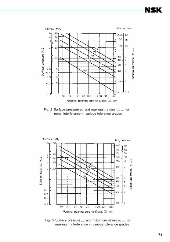
70 71

Fig. 2　Surface pressure pm and maximum stress σt max for 　mean interference in various tolerance grades

Fig. 3　Surface pressure pm and maximum stress σt max for maximum interference in various tolerance grades

72


3.6 Mounting and withdrawal loads

The push-up load needed to mount bearings on shafts or in a housing hole with interference can be obtained using the thick-walled cylinder theory.

The mounting load (or withdrawal load) depends upon the contact area, surface pressure, and coefficient of friction between the fitting surfaces.

The mounting load (or withdrawal load) K needed to mount inner rings on shafts is given by Equation (1).

K=m pm p d B (N), {kgf} .............................. (1)

where m: Coefficient of friction between fitting surfaces

m=0.12 (for mounting) m=0.18 (for withdrawal) pm: Surface pressure (MPa), {kgf/mm2} For example, inner ring surface

pressure can be obtained using Table 1 (Page 69)

pm=

d: Shaft diameter (mm) B: Bearing width (mm) Dd: Effective interference (mm) E: Young’s modulus of steel (MPa),

{kgf/mm2} E=208 000 MPa {21 200 kgf/mm2} k: Inner ring thickness ratio k=d/Di

Di: Inner ring raceway diameter (mm) k0: Hollow shaft thickness ratio k0=d0/d d0: Bore diameter of hollow shaft (mm)

For solid shafts, d0=0, consequently k0=0. The value of k varies depending on the bearing type and size, but it usually ranges between k=0.7 and 0.9. Assuming that k=0.8 and the shaft is solid, Equation (1) is:

K = 118 000m Dd B (N) ........................... (2)

= 12 000m Dd B {kgf}

Equation (2) is shown graphically in Fig. 1. The mounting and withdrawal loads for outer rings and housings have been calculated and the results are shown in Fig. 2.

The actual mounting and withdrawal loads can become much higher than the calculated values if the bearing ring and shaft (or housing) are slightly misaligned or the load is applied unevenly to the circumference of the bearing ring hole. Consequently, the loads obtained from Figs. 1 and 2 should be considered only as guides when designing withdrawal tools, their strength should be five to six times higher than that indicated by the figures.

E2

Ddd

(1–k2) (1–k02)

1–k2 k02

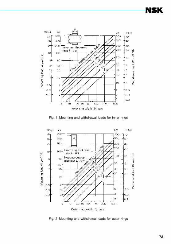
72 73

B

B

Fig. 1　Mounting and withdrawal loads for inner rings

Fig. 2　Mounting and withdrawal loads for outer rings

B

B

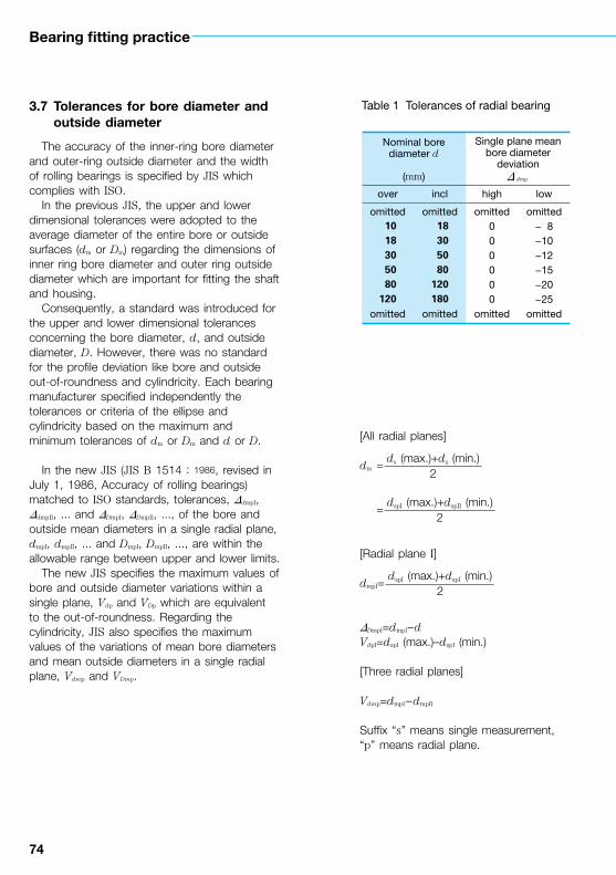
74


3.7 Tolerances for bore diameter and outside diameter

The accuracy of the inner-ring bore diameter and outer-ring outside diameter and the width of rolling bearings is specified by JIS which complies with ISO.

In the previous JIS, the upper and lower dimensional tolerances were adopted to the average diameter of the entire bore or outside surfaces (dm or Dm) regarding the dimensions of inner ring bore diameter and outer ring outside diameter which are important for fitting the shaft and housing.

Consequently, a standard was introduced for the upper and lower dimensional tolerances concerning the bore diameter, d, and outside diameter, D. However, there was no standard for the profile deviation like bore and outside out-of-roundness and cylindricity. Each bearing manufacturer specified independently the tolerances or criteria of the ellipse and cylindricity based on the maximum and minimum tolerances of dm or Dm and d or D.

In the new JIS (JIS B 1514 : 1986, revised in July 1, 1986, Accuracy of rolling bearings) matched to ISO standards, tolerances, DdmpI, DdmpII, ... and DDmpI, DDmpII, ..., of the bore and outside mean diameters in a single radial plane, dmpI, dmpII, ... and DmpI, DmpII, ..., are within the allowable range between upper and lower limits.

The new JIS specifies the maximum values of bore and outside diameter variations within a single plane, Vdp and VDp which are equivalent to the out-of-roundness. Regarding the cylindricity, JIS also specifies the maximum values of the variations of mean bore diameters and mean outside diameters in a single radial plane, Vdmp and VDmp.

[All radial planes]

dm =

=

[Radial plane I]

dmpI=

DDmpI=dmpI–dVdpI=dspI (max.)–dspI (min.)

[Three radial planes]

Vdmp=dmpI –dmpII

Suffix “s” means single measurement, “p” means radial plane.

ds (max.)+ds (min.)2

dspI (max.)+dspII (min.)2

dspI (max.)+dspI (min.)2

Table 1 Tolerances of radial bearing

Nominal borediameter d

(mm)

Single plane meanbore diameter

deviationD dmp

over incl high low

omitted 10 18 30 50 80120

omitted

omitted 18 30 50 80120180

omitted

omitted000000

omitted

omitted− 8−10−12−15−20−25

omitted

74 75

Note ( 1 )　Applicable to individual rings manufactured for combined bearings.

inner rings (Accuracy Class 0) except tapered roller bearings

Diameter series Mean borediametervariation

Vdmp

Radialrunout ofinner ring

Kia

Single bearing Matched set bearing(1) Inner ringwidth

variationVBs

7, 8, 9 0, 1 2, 3, 4 Deviation of inner or outer ring widthD Bs ( orD Cs )Bore diameter variation in a plane Vdp

max. max. max. high low high low max.

omitted101315192531

omitted

omitted 81012192531

omitted

omitted 6 8 9111519

omitted

omitted 6 8 9111519

omitted

omitted101315202530

omitted

omitted000000

omitted

omitted−120−120−120−150−200−250

omitted

omitted000000

omitted

omitted−250−250−250−380−380−500

omitted

omitted202020252530

omitted

Units: mm

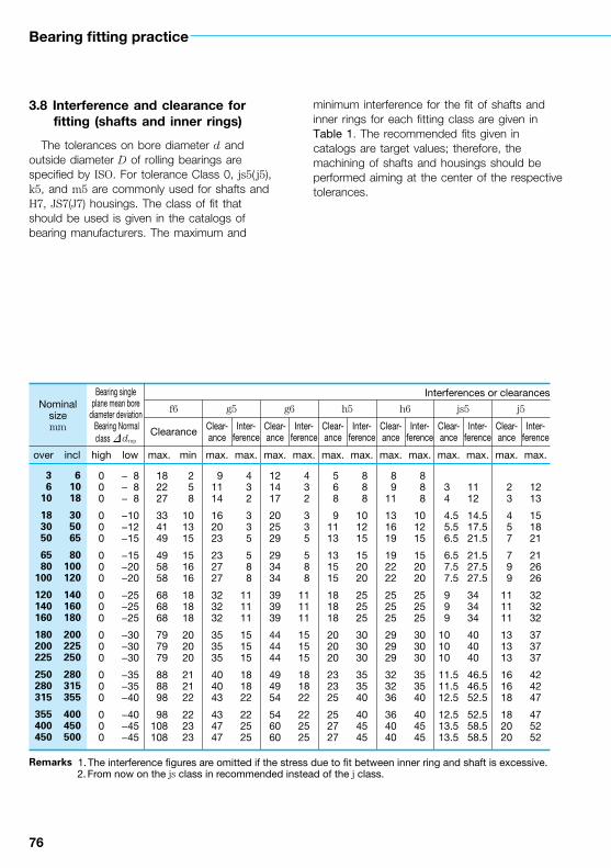
76


3.8 Interference and clearance for fitting (shafts and inner rings)

The tolerances on bore diameter d and outside diameter D of rolling bearings are specified by ISO. For tolerance Class 0, js5( j5), k5, and m5 are commonly used for shafts and H7, JS7(J7) housings. The class of fit that should be used is given in the catalogs of bearing manufacturers. The maximum and

minimum interference for the fit of shafts and inner rings for each fitting class are given in Table 1. The recommended fits given in catalogs are target values; therefore, the machining of shafts and housings should be performed aiming at the center of the respective tolerances.

Remarks 1.　The interference figures are omitted if the stress due to fit between inner ring and shaft is excessive. 2.　From now on the js class in recommended instead of the j class.

Nominalsize　mm　

Bearing singleplane mean bore

diameter deviation　Bearing　 Normalclass　 Ddmp

Interferences or clearances

f6 g5 g6 h5 h6 js5 j5

Clearance Clear-ance

Inter-ference

Clear-ance

Inter-ference

Clear-ance

Inter-ference

Clear-ance

Inter-ference

Clear-ance

Inter-ference

Clear-ance

Inter-ference

over incl high low max. min max. max. max. max. max. max. max. max. max. max. max. max.

3 6 10

18 30 50

65 80100

120140160

180200225

250280315

355400450

6 10 18

30 50 65

80100120

140160180

200225250

280315355

400450500

000

000

000

000

000

000

000

− 8− 8− 8

−10−12−15

−15−20−20

−25−25−25

−30−30−30

−35−35−40

−40−45−45

18 22 27

33 41 49

49 58 58

68 68 68

79 79 79

88 88 98

98108108

2 5 8

101315

151616

181818

202020

212122

222323

91114

162023

232727

323232

353535

404043

434747

4 3 2

3 3 5

5 8 8

111111

151515

181822

222525

121417

202529

293434

393939

444444

494954

546060

4 3 2

3 3 5

5 8 8

111111

151515

181822

222525

5 6 8

91113

131515

181818

202020

232325

252727

8 8 8

101215

152020

252525

303030

353540

404545

8 911

131619

192222

252525

292929

323236

364040

8 8 8

101215

152020

252525

303030

353540

404545

　34

4.55.56.5

6.57.57.5

999

101010

11.511.512.5

12.513.513.5

　1112

14.517.521.5

21.527.527.5

343434

404040

46.546.552.5

52.558.558.5

　 2 3

4 5 7

7 9 9

111111

131313

161618

182020

　1213

151821

212626

323232

373737

424247

475252

76 77

Units: mm

for each shaft toleranceNominal

size　mm　

js6 j6 k5 k6 m5 m6 n6 p6 r6

Clear-ance

Interfer-ence

Clear-ance

Interfer-ence Interference Interference Interference Interference Interference Interference Interference

max. max. max. max. min. max. min. max. min. max. min. max. min. max. min. max. min. max. over incl

　4.55.5

6.589.5

9.51111

12.512.512.5

14.514.514.5

161618

182020

　12.513.5

16.52024.5

24.53131

37.537.537.5

44.544.544.5

515158

586565

　 2 3

4 5 7

7 9 9

111111

131313

161618

182020

　1516

192327

273333

393939

464646

515158

586565

　　　

222

233

333

444

444

455

　　　

212530

303838

464646

545454

626269

697777

　　　

222

233

333

444

444

455

　　　

253036

364545

535353

636363

717180

809090

　　　

　 911

111313

151515

171717

202021

212323

　　　

　3239

394848

585858

676767

787886

869595

　　　

　 911

111313

151515

171717

202021

212323

　　　

　 37 45

45 55 55

65 65 65

76 76 76

87 87 97

97108108

　　　

　　　

202323

272727

313131

343437

374040

　　　

　　　

54 65 65

77 77 77

90 90 90

101101113

113125125

　　　

　　　

　3737

434343

505050

565662

626868

　　　

　　　

　 79 79

93 93 93

109109109

123123138

138153153

　　　

　　　

　　　

63 65 68

77 80 84

94 98108

114126132

　　　

　　　

　　　

113115118

136139143

161165184

190211217

3 6 10

18 30 50

65 80100

120140160

180200225

250280315

355400450

6 10 18

30 50 65

80100120

140160180

200225250

280315355

400450500

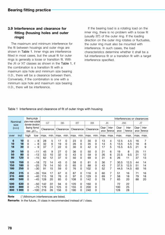
78


3.9 Interference and clearance for fitting (housing holes and outer rings)

The maximum and minimum interference for the fit between housings and outer rings are shown in Table 1. Inner rings are interference fitted in most cases, but the usual fit for outer rings is generally a loose or transition fit. With the J6 or N7 classes as shown in the Table 1, if the combination is a transition fit with a maximum size hole and minimum size bearing O.D., there will be a clearance between them. Conversely, if the combination is one with a minimum size hole and maximum size bearing O.D., there will be interference.

If the bearing load is a rotating load on the inner ring, there is no problem with a loose fit (usually H7) of the outer ring. If the loading direction on the outer ring rotates or fluctuates, the outer ring must also be mounted with interference. In such cases, the load characteristics determine whether it shall be a full interference fit or a transition fit with a target interference specified.

Note ( 1 )　Minimum interferences are listed.Remarks In the future, JS class in recommended instead of J class.

Table 1 Interference and clearance of fit of outer rings with housing

Nominalsize(mm)

Bearing single plane mean outside diameter deviation 　Bearing: Normal class　 DDmp

Interferences or clearances

G7 H6 H7 H8 J6 JS6 J7

Clearance Clearance Clearance Clearance Clear-ance

Inter-ference

Clear-ance

Inter-ference

Clear-ance

Inter-ference

over incl high low max. min. max. min. max. min. max. min. max. max. max. max. max. max.

6 10 18

30 50 80

120150180

250315400

500630800

10 18 30

50 80 120

150 180 250

315 400 500

630 8001 000

000

000

000

000

000

− 8 − 8 − 9

−11 −13 −15

−18 −25 −30

−35 −40 −45

−50 −75−100

28 32 37

45 53 62

72 79 91

104115128

142179216

5 6 7

91012

141415

171820

222426

17 19 22

27 32 37

43 50 59

67 76 85

94125156

000

000

000

000

000

23 26 30

36 43 50

58 65 76

87 97108

120155190

000

000

000

000

000

30 35 42

50 59 69

81 88102

116129142

160200240

000

000

000

000

000

131417

212631

364352

606978

　　　

455

666

777

777

　　　

12.513.515.5

1922.526

30.537.544.5

515865

72100128

4.55.56.5

89.5

11

12.512.514.5

161820

222528

161821

253137

445160

717988

　　　

7 8 9

111213

141416

161820

　　　

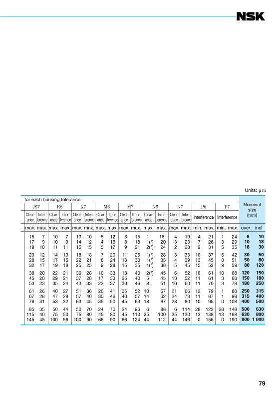
78 79

Units: mm

for each housing toleranceNominal

size(mm)

JS7 K6 K7 M6 M7 N6 N7 P6 P7

Clear-ance

Inter-ference

Clear-ance

Inter-ference

Clear-ance

Inter-ference

Clear-ance

Inter-ference

Clear-ance

IInter-ference

Clear-ance

Inter-ference

Clear-ance

Inter-ference Interference Interference

max. max. max. max. max. max. max. max. max. max. max. max. max. max. min. max. min. max. over incl

15 17 19

23 28 32

38 45 53

61 67 76

85115145

7 910

121517

202023

262831

354045

10 10 11

14 17 19

22 29 35

40 47 53

50 75100

7 911

131518

212124

272932

445056

13 14 15

18 22 25

30 37 43

51 57 63

50 75100

101215

182125

282833

364045

708090

5 4 5

7 8 9

101722

263035

244566

121517

202428

333337

414650

708090

8 8 9

111315

182530

354045

244566

15 18 21

25 30 35

40 40 46

52 57 63

96110124

11(1)2(1)

1(1)1(1)1(1)

2(1)58

101418

62544

16 20 24

28 33 38

45 45 51

57 62 67

88100112

4 3 2

3 4 5

61316

212428

62544

19 23 28

33 39 45

52 52 60

66 73 80

114130146

4 7 9

101315

181111

121110

2813 0

21 26 31

37 45 52

61 61 70

79 87 95

122138156

1 3 5

6 8 9

10 3 3

1 1 0

2813 0

24 29 35

42 51 59

68 68 79

88 98108

148168190

6 10 18

30 50 80

120150180

250315400

500630800

10 18 30

50 80 120

150 180 250

315 400 500

630 8001 000

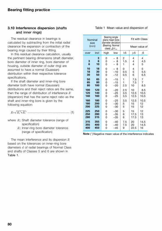
80


3.10 Interference dispersion (shafts and inner rings)

The residual clearance in bearings is calculated by subtracting from the initial radial clearance the expansion or contraction of the bearing rings caused by their fitting.

In this residual clearance calculation, usually the pertinent bearing dimensions (shaft diameter, bore diameter of inner ring, bore diameter of housing, outside diameter of outer ring) are assumed to have a normal (Guassian) distribution within their respective tolerance specifications.

If the shaft diameter and inner-ring bore diameter both have normal (Gaussian) distributions and their reject ratios are the same, then the range of distribution of interference R (dispersion) that has the same reject ratio as the shaft and inner-ring bore is given by the following equation:

R= Rs2+Ri

2 ................................................. (1)

where Rs: Shaft diameter tolerance (range of specification)

Ri: Inner-ring bore diameter tolerance (range of specification)

The mean interference and its dispersion R based on the tolerances on inner-ring bore diameters d of radial bearings of Normal Class and shafts of Classes 5 and 6 are shown in Table 1.

√————

Note ( 1 )　Negative mean value of the interference indicates

Table 1 Mean value and dispersion of

Nominalsize(mm)

Bearing singleplane mean bore

diameter deviation(Bearing: Normal

class) Ddmp

Fit with Class

Mean value of

over incl high low h5 js5 j5

　 3 6

10 18 30

50 65 80

100120140

160180200

225250280

315355400

3 6 10

18 30 50

65 80100

120140160

180200225

250280315

355400450

000

000

000

000

000

000

000

− 8− 8− 8

− 8−10−12

−15−15−20

−20−25−25

−25−30−30

−30−35−35

−40−40−45

21.51

00.50.5

112.5

2.53.53.5

3.555

566

7.57.59

444

456

7.57.5

10

1012.512.5

12.51515

1517.517.5

202022.5

44.55

55.56.5

778.5

8.510.510.5

10.51212

121313

14.514.516

80 81

clearance.

interference for fitting of inner rings with shaftsUnits: mm

5 shaft Fit with Class 6 shaft

interference Dispersion ofinterference

R　 Rs2　Ri

2

Mean value of interference (1) Dispersion ofinterference

R　 Rs2　Ri

2k5 m5 h6 js6 j6 k6 m6 n6 p6 r6

67.58

911.513.5

161620.5

20.524.524.5

24.52929

293333

36.536.541

810.513

1517.520.5

252530.5

30.536.536.5

36.54242

424949

53.553.559

± 4.5± 4.5± 5

± 5.5± 6.5± 8

±10±10±12.5

±12.5±15.5±15.5

±15.5±18±18

±18±21±21

±23.5±23.5±26

10

−0.5

−1.5−1.5−2

−2−2−1

−100

00.50.5

0.51.51.5

222.5

444

456

7.57.5

10

1012.512.5

12.51515

1517.517.5

202022.5

566.5

6.57.59

101012

121414

1416.516.5

16.517.517.5

202022.5

799.5

10.513.516

191924

242828

2833.533.5

33.537.537.5

424247.5

91214.5

16.519.523

282834

344040

4046.546.5

46.553.553.5

595965.5

111618.5

21.526.531

373744

445252

5260.560.5

60.567.567.5

757582.5

132023.5

27.533.540

494958

586868

6879.579.5

79.589.589.5

100100110.5

172327.5

32.539.548

586072

758890

93106.5109.5

113.5127.5131.5

146152168.5

± 5± 5.5± 6

± 7± 8±10

±12±12±15

±15±17.5±17.5

±17.5±21±21

±21±23.5±23.5

±27±27±30

82


3.11 Interference dispersion (housing bores and outer rings)

In a manner similar to the previous interference dispersion for shafts and inner rings, that for housings and outer rings is shown in Table 1. The interference dispersion R in Table 1 is given by the following equation:

R= Re2+RH

2 ................................................. (1)

where Re: Tolerance on outside diameter of outer ring (range of specification value)

RH: Tolerance on bore diameter of housing (range of specification value)

This is based on the property that the sum of two or more numbers, which are normally distributed, is also distributed normally (rule for the addition of Gaussian distributions).

Table 1 shows the mean value and dispersion R of interference for the fitting of radial bearings of Normal Class and housings of Classes 6 and 7.

This rule for the addition of Gaussian distributions is widely used for calculating residual clearance and estimating the overall dispersion of a series of parts which are within respective tolerance ranges.

√————

Note ( 1 )　Negative mean value of the interference indicates

Table 1 Mean value and dispersion of

Nominalsize(mm)

Bearing singleplane mean outsidediameter deviation(Bearing: Normal

class) DDmp

Fit with

Mean value

over incl high low H6 J6 JS6

3 6 10

18 30 50

80120150

180250315

400500630

800

6 10 18

30 50 80

120 150 180

250 315 400

500 630 800

1000

000

000

000

000

000

0

− 8− 8− 8

− 9− 11− 13

− 15− 18− 25

− 30− 35− 40

− 45− 50− 75

−100

− 8− 8.5− 9.5

−11−13.5−16

−18.5−21.5−25

−29.5−33.5−38

−42.5−47−62.5

−78

− 5− 4.5− 4.5

− 6− 7.5−10

−12.5−14.5−18

−22.5−26.5−31

−35.5　　

　

− 4− 4− 4

− 4.5− 5.5− 6.5

− 7.5− 9−12.5

−15−17.5−20

−22.5−25−37.5

−50

82 83

clearance.

interference for the fitting of outer rings with housingsUnits: mm

Class 6 housing Fit with Class 7 housing

of interference (1) Dispersion ofinterferenceR= Re

2　RH2

Mean value of interference (1) Dispersion ofinterferenceR= Re

2　RH2

K6 M6 N6 P6 H7 J7 JS7 K7 M7 N7 P7

− 2− 1.5− 0.5

0− 0.5− 1

− 0.5− 0.5− 4

− 5.5− 6.5− 9

−10.5− 3−12.5

−22

13.55.5

66.58

9.511.5

8

7.57.58

7.52317.5

12

57.5

10.5

1314.517

19.523.520

21.523.524

24.54137.5

34

912.516.5

2023.529

33.539.536

40.545.549

52.57575.5

78

± 5.5± 6± 7

± 8± 9.5±11.5

±13.5±15.5±17.5

±21±23.5±27

±30±33.5±45

±57.5

−10−11.5−13

−15−18−21.5

−25−29−32.5

−38−43.5−48.5

−54−60−77.5

−95

− 4− 4.5− 5

− 6− 7− 9.5

−12−15−18.5

−22−27.5−30.5

−34　　

　

− 4− 4− 4

− 4.5− 5.5− 6.5

− 7.5− 9−12.5

−15−17.5−20

−22.5−25−37.5

−50

− 1− 1.5− 1

00

− 0.5

0− 1− 4.5

− 5− 7.5− 8.5

− 910

2.5

− 5

23.55

678.5

1011

7.5

88.58.5

93632.5

29

67.5

10

131517.5

202319.5

2222.524.5

265452.5

51

1012.516

202429.5

343935.5

4144.549.5

548890.5

95

± 7± 8.5±10

±11.5±13.5±16.5

±19±22±23.5

±27.5±31.5±35

±38.5±43±55

±67

84


3.12 Fits of four-row tapered roller bearings (metric) for roll necks

Bearings of various sizes and types are used in steel mill rolling equipment, such as rolling rolls, reducers, pinion stands, thrust blocks, table rollers, etc. Among them, roll neck bearings are the ones which must be watched most closely because of their severe operating conditions and their vital role.

As a rule for rolling bearing rings, a tight fit should be used for the ring rotating under a load. This rule applies for roll neck bearings, the fit of the inner ring rotating under the load should be tight.

However, since the rolls are replaced frequently, mounting and dismounting of the bearings on the roll necks should be easy. To meet this requirement, the fit of the roll neck and bearing is loose enabling easy handling. This means that the inner ring of the roll neck bearing which sustains relatively heavy load, may creep resulting in wear or score on the roll neck surface. Therefore, the fitting of the roll neck and bearing should have some clearance and a lubricant (with an extreme pressure additive) is applied to the bore surface to create a protective oil film.

If a loose fit is used, the roll neck tolerance should be close to the figures listed in Table 1. Compared with the bearing bore tolerance, the clearance of the fit is much larger than that of a loose fit for general rolling bearings.

The fit between the bearing outer ring and chock (housing bore) is also a loose fit as shown in Table 2.

Even if the clearance between the roll neck and bearing bore is kept within the values in Table 1, steel particles and dust in the fitting clearance may roughen the fitting surface.

Roll neck bearings are inevitably mounted with a loose fit to satisfy easy mounting/dismounting. If the roll neck bearing replacement interval is long, a tight fit is preferable.

Some rolling mills use tapered roll necks. In this case, the bearing may be mounted and dismounted with a hydraulic device.

Also, there are some rolling mills that use four-row cylindrical roller bearings where the inner ring is tightly fitted with the roll neck. By the way, inner ring replacement is easier if an induction heating device is used.

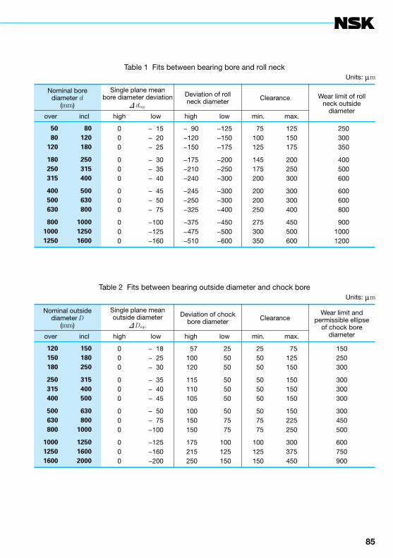
84 85

Table 1 Fits between bearing bore and roll neckUnits: mm

Nominal borediameter d

(mm)

Single plane meanbore diameter deviation

D dmp

Deviation of roll neck diameter Clearance Wear limit of roll

neck outside diameter

over incl high low high low min. max.

50 80 120

180 250 315

400 500 630

80010001250

80 120 180

250 315 400

500 630 800

100012501600

000

000

000

000

− 15− 20− 25

− 30− 35− 40

− 45− 50− 75

−100−125−160

− 90−120−150

−175−210−240

−245−250−325

−375−475−510

−125−150−175

−200−250−300

−300−300−400

−450−500−600

75100125

145175200

200200250

275300350

125150175

200250300

300300400

450500600

250 300 350

400 500 600

600 600 800

90010001200

Table 2 Fits between bearing outside diameter and chock boreUnits: mm

Nominal outsidediameter D

(mm)

Single plane meanoutside diameter

D Dmp

Deviation of chockbore diameter Clearance

Wear limit andpermissible ellipse

of chock borediameterover incl high low high low min. max.

120 150 180

250 315 400

500 630 800

100012501600

150 180 250

315 400 500

630 8001000

125016002000

000

000

000

000

− 18− 25− 30

− 35− 40− 45

− 50− 75−100

−125−160−200

　 57　100　120

　115　110　105

　100　150　150

　175　215　250

　 25　 50　 50

　 50　 50　 50

　 50　 75　 75

　100　125　150

25 50 50

50 50 50

50 75 75

100125150

75125150

150150150

150225250

300375450

150250300

300300300

300450500

600750900

86

4. Internal clearance

4.1 Internal clearance

Internal clearance is one of the most important factors affecting bearing performance. The bearing “internal clearance” is the relative movement of the outer and inner rings when they are lightly pushed in opposite directions. Movement in the diametrical direction is called radial clearance and that in the shaft’s direction is called axial clearance.

The reason why the internal clearance is so important for bearings is that it is directly related to their performance in the following respects. The amount of clearance influences the load distribution in a bearing and this can affect its life. It also influences the noise and vibration. In addition, it can influence whether the rolling elements move by rolling or sliding motion.

Normally, bearings are installed with interference for either the inner or outer ring and this leads to its expansion or contraction which causes a change in the clearance. Also, the bearing temperature reaches saturation during operation; however, the temperature of the inner ring, outer ring, and rolling elements are all different from each other, and this temperature difference changes the clearance (Fig. 1). Moreover, when a bearing operates under load, an elastic displacement of the inner ring, outer ring, and rolling elements also leads to a change in clearance. Because of these changes, bearing internal clearance is a very complex subject.

Therefore, what is the ideal clearance? Before considering this question, let us define the following different types of clearance. The symbol for each clearance amount is shown in parentheses.

Measured Internal Clearance (D1)This is the internal clearance measured under a specified measuring load and can be called “apparent clearance”. This clearance includes the elastic deformation (dFO) caused by the measuring load.

D1=D0+dFO

Theoretical Internal Clearance (D0)This is the radial internal clearance which is the measured clearance minus the elastic deformation caused by the measuring load.

D0=D1+dFO

dFO is significant for ball bearings, but not for roller bearings where it is assumed to be equal to zero, and thus, D0=D1.

Residual Internal Clearance (Df)This is the clearance left in a bearing after mounting it on a shaft and in a housing. The elastic deformation caused by the mass of the shaft, etc. is neglected. Assuming the clearance decrease caused by the ring expansion or contraction is df, then:

Df=D0+df

Effective Internal Clearance (D)This is the bearing clearance that exists in a machine at its operating temperature except that the elastic deformation caused by load is not included. That is to say, this is the clearance when considering only the changes due to bearing fitting df and temperature difference between the inner and outer rings dt. The basic load ratings of bearings apply only when the effective clearance D=0.

D=Df–dt=D0–(df+dt)

Operating Clearance (DF)This is the actual clearance when a bearing is installed and running under load. Here, the effect of elastic deformation dF is included as well as fitting and temperature. Generally, the operating clearance is not used in the calculation.

DF=D+dF

86 87

The most important clearance of a bearing is the effective clearance as we have already explained. Theoretically speaking, the bearing whose effective clearance D is slightly negative has the longest life. (The slightly negative clearance means such effective clearance that the operating clearance turns to positive by the influence of bearing load. Strictly speaking, the amount of negative clearance varies with the magnitude of bearing load.) However, it is impossible to make the clearance of all bearings to the ideal effective clearance, and we have to

consider the geometrical clearance D0 in order to let the minimum value of effecive clearance be zero or a slightly negative value. To obtain this value, we should have both accurate reduction amount of clearance caused by the interference of the inner ring and outer ring df and accurate amount of clearance change caused by the temperature difference between inner ring and outer ring dt. The methods of the calculation are discussed in the following sections.

Roller

Outer ring

Fig. 1　Changes of radial internal clearance of roller bearing

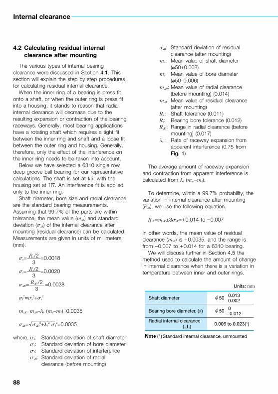
88

Internal clearance

4.2 Calculating residual internal clearance after mounting

The various types of internal bearing clearance were discussed in Section 4.1. This section will explain the step by step procedures for calculating residual internal clearance.

When the inner ring of a bearing is press fit onto a shaft, or when the outer ring is press fit into a housing, it stands to reason that radial internal clearance will decrease due to the resulting expansion or contraction of the bearing raceways. Generally, most bearing applications have a rotating shaft which requires a tight fit between the inner ring and shaft and a loose fit between the outer ring and housing. Generally, therefore, only the effect of the interference on the inner ring needs to be taken into account.

Below we have selected a 6310 single row deep groove ball bearing for our representative calculations. The shaft is set at k5, with the housing set at H7. An interference fit is applied only to the inner ring.

Shaft diameter, bore size and radial clearance are the standard bearing measurements. Assuming that 99.7% of the parts are within tolerance, the mean value (mDf) and standard deviation (sDf) of the internal clearance after mounting (residual clearance) can be calculated. Measurements are given in units of millimeters (mm).

ss= =0.0018

si= =0.0020

sD0= =0.0028

sf2=ss

2+si2

mDf=mD0–li (ms–mi)=0.0035

sDf= sD02+li

2 sf2=0.0035

where, ss: Standard deviation of shaft diameter si: Standard deviation of bore diameter sf: Standard deviation of interference sD0: Standard deviation of radial

clearance (before mounting)

sDf: Standard deviation of residual clearance (after mounting)

ms: Mean value of shaft diameter (f50+0.008)

mi: Mean value of bore diameter (f50–0.006)

mD0: Mean value of radial clearance (before mounting) (0.014)

mDf: Mean value of residual clearance (after mounting)

Rs: Shaft tolerance (0.011) Ri: Bearing bore tolerance (0.012) RD0: Range in radial clearance (before

mounting) (0.017) li: Rate of raceway expansion from

apparent interference (0.75 from Fig. 1)

The average amount of raceway expansion and contraction from apparent interference is calculated from li (mm–mi).

To determine, wihtin a 99.7% probability, the variation in internal clearance after mounting (RDf), we use the following equation.

RDf=mDf±3sDf=+0.014 to –0.007

In other words, the mean value of residual clearance (mDf) is +0.0035, and the range is from –0.007 to +0.014 for a 6310 bearing.

We will discuss further in Section 4.5 the method used to calculate the amount of change in internal clearance when there is a variation in temperature between inner and outer rings.

Rs/23

Ri/23

RD0/23

√——————

Note ( 1 )　Standard internal clearance, unmounted

Units: mm

Shaft diameter 　0.013φ50 　0.002

Bearing bore diameter, (d) 　0φ50 −0.012

Radial internal clearance (D 0)

0.006 to 0.023(1)

88 89

Fig. 1　Rate of inner ring raceway expansion (li) from apparent interference

Fig. 2　Distribution of residual internal clearance

90

Internal clearance

4.3 Effect of interference fit on bearing raceways (fit of inner ring)

One of the important factors that relates to radial clearance is the reduction in radial clearance resulting from the mounting fit. When inner ring is mounted on a shaft with an interference fit and the outer ring is secured in a housing with an interference fit, the inner ring will expand and the outer ring will contract.

The means of calculating the amount of ring expansion or contraction were previously noted in Section 3.4, however, the equation for establishing the amount of inner raceway expansion (DDi) is given in Equation (1).

DDi=Dd k ................................. (1)

where, Dd: Effective interference (mm) k: Ratio of bore to inner raceway

diameter; k=d/Di

k0: Ratio of inside to outside diameter of hollow shaft; k0=d0/Di

d: Bore or shaft diameter (mm) Di: Inner raceway diameter (mm) d0: Inside diameter of hollow shaft (mm)

Equation (1) has been translated into a clearer graphical form in Fig. 1.

The vertical axis of Fig. 1 represents the inner raceway diameter expansion in relation to the amount of interference. The horizontal axis is the ratio of inside and outside diameter of the hollow shaft (k0) and uses as its parameter the ratio of bore diameter and raceway diameter of the inner ring (k).

Generally, the decrease in radial clearance is calculated to be approximately 80% of the interference. However, this is for solid shaft mountings only. For hollow shaft mountings the decrease in radial clearance varies with the ratio of inside to outside diameter of the shaft. Since the general 80% rule is based on average bearing bore size to inner raceway diameter ratios, the change will vary with different bearing types, sizes, and series. Typical plots for Single Row Deep Groove Ball Bearings and for

Cylindrical Roller Bearings are shown in Figs. 2 and 3. Values in Fig. 1 apply only for steel shafts.

Let’s take as an example a 6220 ball bearing mounted on a hollow shaft (diameter d=100 mm, inside diameter d0=65 mm) with a fit class of m5 and determine the decrease in radial clearance.

The ratio between bore diameter and raceway diameter, k is 0.87 as shown in Fig. 2. The ratio of inside to outside diameter for shaft, k0, is k0=d0/d=0.65. Thus, reading from Fig. 1, the rate of raceway expansion is 73%.

Given that an interference of m5 has a mean value of 30 mm, the amount of raceway expansion, or, the amount of decrease in the radial clearance from the fit is 0.73×30=22 mm.

1–k02

1–k2 k02

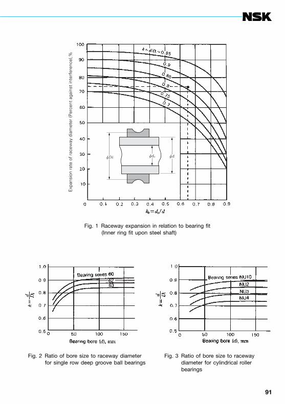
90 91

φdφDi φd0

Exp

ansi

on r

ate

of r

acew

ay d

iam

eter

(Per

cent

aga

inst

inte

rfer

ence

),%

Fig. 1　Raceway expansion in relation to bearing fit (Inner ring fit upon steel shaft)

Fig. 2　Ratio of bore size to raceway diameter for single row deep groove ball bearings

Fig. 3　Ratio of bore size to raceway diameter for cylindrical roller bearings

φdφDi φd0

Exp

ansi

on r

ate

of r

acew

ay d

iam

eter

(Per

cent

aga

inst

inte

rfer

ence

),%

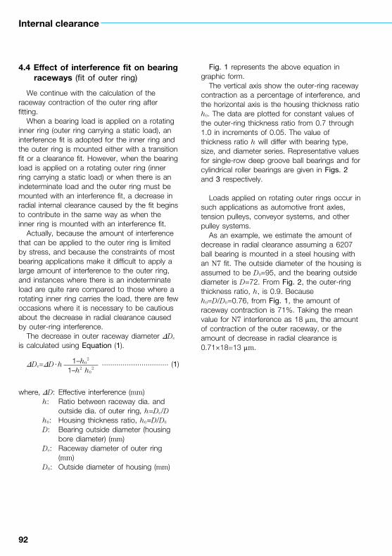
92

Internal clearance

4.4 Effect of interference fit on bearing raceways (fit of outer ring)

We continue with the calculation of the raceway contraction of the outer ring after fitting.

When a bearing load is applied on a rotating inner ring (outer ring carrying a static load), an interference fit is adopted for the inner ring and the outer ring is mounted either with a transition fit or a clearance fit. However, when the bearing load is applied on a rotating outer ring (inner ring carrying a static load) or when there is an indeterminate load and the outer ring must be mounted with an interference fit, a decrease in radial internal clearance caused by the fit begins to contribute in the same way as when the inner ring is mounted with an interference fit.

Actually, because the amount of interference that can be applied to the outer ring is limited by stress, and because the constraints of most bearing applications make it difficult to apply a large amount of interference to the outer ring, and instances where there is an indeterminate load are quite rare compared to those where a rotating inner ring carries the load, there are few occasions where it is necessary to be cautious about the decrease in radial clearance caused by outer-ring interference.

The decrease in outer raceway diameter DDe is calculated using Equation (1).

DDe=DD ·h ................................ (1)

where, DD: Effective interference (mm) h: Ratio between raceway dia. and

outside dia. of outer ring, h=De/D h0: Housing thickness ratio, h0=D/D0

D: Bearing outside diameter (housing bore diameter) (mm)

De: Raceway diameter of outer ring (mm)

D0: Outside diameter of housing (mm)

Fig. 1 represents the above equation in graphic form.

The vertical axis show the outer-ring raceway contraction as a percentage of interference, and the horizontal axis is the housing thickness ratio h0. The data are plotted for constant values of the outer-ring thickness ratio from 0.7 through 1.0 in increments of 0.05. The value of thickness ratio h will differ with bearing type, size, and diameter series. Representative values for single-row deep groove ball bearings and for cylindrical roller bearings are given in Figs. 2 and 3 respectively.

Loads applied on rotating outer rings occur in such applications as automotive front axles, tension pulleys, conveyor systems, and other pulley systems.

As an example, we estimate the amount of decrease in radial clearance assuming a 6207 ball bearing is mounted in a steel housing with an N7 fit. The outside diameter of the housing is assumed to be D0=95, and the bearing outside diameter is D=72. From Fig. 2, the outer-ring thickness ratio, h, is 0.9. Because h0=D/D0=0.76, from Fig. 1, the amount of raceway contraction is 71%. Taking the mean value for N7 interference as 18 mm, the amount of contraction of the outer raceway, or the amount of decrease in radial clearance is 0.71×18=13 mm.

1–h02

1–h2 h02

92 93

φD φDe φD0

Con

trac

tion

rate

of

race

way

dia

met

er (P

erce

nt a

gain

st in

terf

eren

ce),%

Fig. 1　Raceway contraction in relation to bearing fit (Outer ring fit in steel housing)

Fig. 2　Ratio of outside diameter to raceway diameter for single row deep groove ball bearings

Fig. 3　Ratio of outside diameter to raceway diameter for cylindrical roller bearings

94

Internal clearance

4.5 Reduction in radial internal clearance caused by a temperature difference between inner and outer rings

The internal clearance after mounting was explained in Section 4.2. We continue here by explaining the way to determine the reduction in radial internal clearance caused by inner and outer ring temperature differences and, finally, the method of estimating the effective internal clearance in a systematic fashion.

When a bearing runs under a load, the temperature of the entire bearing will rise. Of course, the rolling elements also undergo a temperature change, but, because the change is extremely difficult to measure or even estimate, the temperature of the rolling elements is generally assumed to be the same as the inner-ring temperature.

We will use the same bearing for our example as we did in Section 4.2, a 6310, and determine the reduction in clearance caused by a temperature difference of 5°C between the inner and outer rings using the equation below.

dt=aDtDe≒aDt ................................... (1)

≒12.5×10–6×5×

≒6×10–3 (mm)

where dt: Decrease in radial internal clearance caused by a temperature difference between the inner and outer rings (mm)

a: Linear thermal expansion coefficient for bearing steel, 12.5×10–6 (1/°C)

Dt: Difference in temperature between inner ring (or rolling elements) and outer ring (°C)

D: Outside diameter (6310 bearing, 110 mm)

d: Bore diameter (6310 bearing, 50 mm) De: Outer-ring raceway diameter (mm)

The following equations are used to calculate the outer-ring raceway diameter:

Ball Bearings: De=(4D+d)/5Roller Bearings: De=(3D+d)/4

Using the values for Df, the residual clearance arrived at in Section 4.2, and for dt, the reduction in radial internal clearance caused by a temperature difference between the inner and outer rings just calculated, we can determine the effective internal clearance (D) using the following equation.D=Df–dt=(+0.014 to –0.007) –0.006

= +0.008 to –0.013

Referring to Fig. 1 below (also see Section 2.8) we can see how the effective internal clearance influences bearing life (in this example with a radial load of 3 350 N {340 kgf}, or approximately 5% of the basic load rating). The longest bearing life occurs under conditions where the effective internal clearance is –13 mm. The lowest limit to the preferred effective internal clearance range is also –13 mm.

To summarize radial internal clearances briefly:(1) Generally, the radial clearances given in

tables and figures are theoretical internal clearances, D0.

(2) The most important clearance for bearings is the effective radial internal clearance, D. It is a value determined by taking the theoretical clearance D0 and subtracting df, the reduction in clearance caused by the interference fit of one or both rings, and dt, the reduction in clearance caused by a temperature difference between the inner and outer rings. D=D0–(df+dt).

(3) Theoretically, the optimum effective internal clearance D is a negative number close to zero which gives maximum bearing life. Therefore, it is desirable for a bearing to have an effective internal clearance greater than the ideal minimum value.

(4) To determine the relation between the effective internal clearance and bearing life (strictly speaking, the bearing load should also be considered), there is actually no need to give serious consideration to

4D+d5

4×110+505

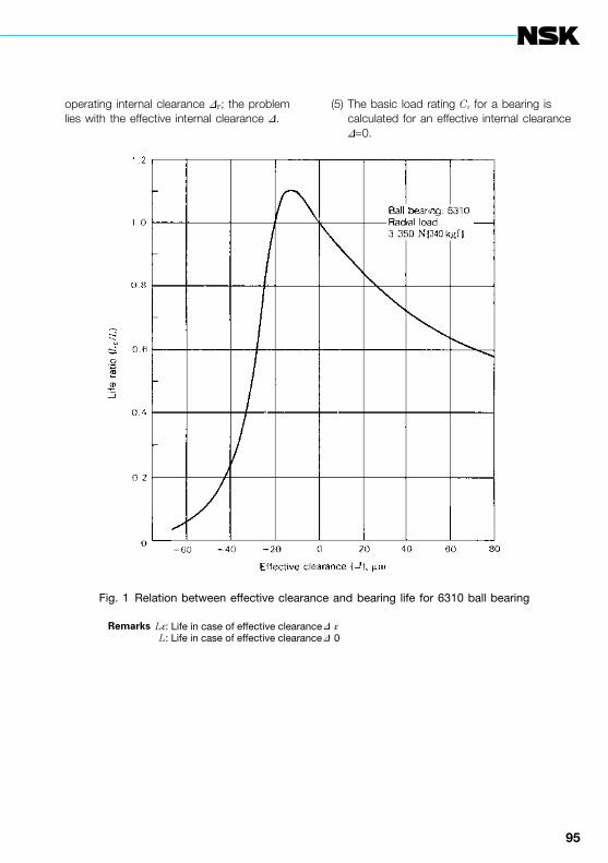
94 95

operating internal clearance DF; the problem lies with the effective internal clearance D.

(5) The basic load rating Cr for a bearing is calculated for an effective internal clearance D=0.

Fig. 1　Relation between effective clearance and bearing life for 6310 ball bearing

Remarks Lε: Life in case of effective clearance D 　ε L: Life in case of effective clearance D 　0

96

Internal clearance

4.6 Radial and axial internal clearances and contact angles for single row deep groove ball bearings

4.6.1 Radial and axial internal clearancesThe internal clearance in single row bearings

has been specified as the radial internal clearance. The bearing internal clearance is the amount of relative displacement possible between the bearing rings when one ring is fixed and the other ring does not bear a load. The amount of movement along the direction of the bearing radius is called the radial clearance, and the amount along the direction of the axis is called the axial clearance.

The geometric relation between the radial and axial clearance is shown in Fig. 1.

Symbols used in Fig. 1Oa: Ball centerOe: Center of groove curvature, outer ringOi: Center of groove curvature, inner ringDw: Ball diameter (mm)re: Radius of outer ring groove (mm)ri: Radius of inner ring groove (mm)a: Contact angle (° )Dr: Radial clearance (mm)Da: Axial clearance (mm)

It is apparent from Fig. 1 that Dr=Dre +Dri.

From geometric relationships, various equations for clearance, contact angle, etc. can be derived.

Dr=2 (1–cos a) (re+ri–Dw) ............................... (1)

Da=2 sin a (re+ri–Dw) ..................................... (2)

=cot .................................................... (3)

Da≒2 (re+ri–Dw)1/2Dr1/2 ...................................... (4)

a=cos–1 ................................ (5)

=sin–1 ......................................... (6)

Because (re+ri–Dw) is a constant, it is apparent why fixed relationships between Dr, Da and a exist for all the various bearing types.

As was previously mentioned, the clearances for deep groove ball bearings are given as radial clearances, but there are specific applications where it is desirable to have an axial clearance as well. The relationship between deep groove ball bearing radial clearance Dr and axial clearance Da is given in Equation (4). To simplify,Da≒K Dr

1/2 ................................................... (7)

where K: Constant depending on bearing design

K=2 (re+ri–Dw)1/2

Fig. 2 shows one example. The various values for K are presented by bearing size in Table 1 below.

ExampleAssume a 6312 bearing, for a sample calculation, which has a radial clearance of 0.017 mm. From Table 1, K=2.09. Therefore, the axial clearance Da is:D=2.09× 0.017=2.09×0.13=0.27 (mm)

Da

Dr

a2

re+ri–Dw–

re+ri–Dw

Dr

2( )Da/2

re+ri–Dw( )

√———

Fig. 1　Relationship Between D r and D a

96 97

Fig. 2　Radial clearance, D r and axial clearance, D a of deep groove ball bearings

Table 1 Constant values of K for radial and axial clearance conversion

Bearingbore No.

K

Series 160 Series 60 Series 62 Series 63

000102030405060708091011121314151617181920212224262830

　0.800.800.800.900.900.960.960.961.011.011.061.061.061.161.161.201.201.291.291.291.371.401.401.541.541.57

　0.800.930.930.960.961.011.061.061.111.111.201.201.201.291.291.371.371.441.441.441.541.641.641.701.701.76

0.930.930.930.991.061.061.071.251.291.291.331.401.501.541.571.571.641.701.761.821.881.952.012.062.112.112.11

1.141.061.061.111.071.201.191.371.451.571.641.702.091.821.881.952.012.062.112.162.252.322.402.402.492.592.59

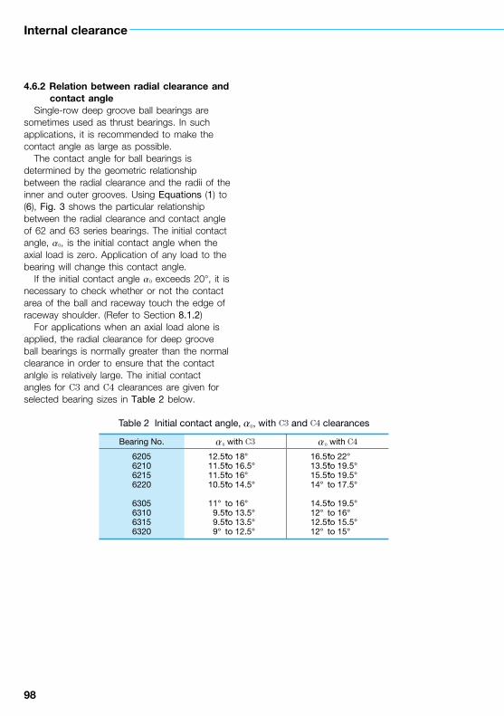
98

Internal clearance

4.6.2 Relation between radial clearance and contact angle

Single-row deep groove ball bearings are sometimes used as thrust bearings. In such applications, it is recommended to make the contact angle as large as possible.

The contact angle for ball bearings is determined by the geometric relationship between the radial clearance and the radii of the inner and outer grooves. Using Equations (1) to (6), Fig. 3 shows the particular relationship between the radial clearance and contact angle of 62 and 63 series bearings. The initial contact angle, a0, is the initial contact angle when the axial load is zero. Application of any load to the bearing will change this contact angle.

If the initial contact angle a0 exceeds 20°, it is necessary to check whether or not the contact area of the ball and raceway touch the edge of raceway shoulder. (Refer to Section 8.1.2)

For applications when an axial load alone is applied, the radial clearance for deep groove ball bearings is normally greater than the normal clearance in order to ensure that the contact anlgle is relatively large. The initial contact angles for C3 and C4 clearances are given for selected bearing sizes in Table 2 below.

Table 2 Initial contact angle, a0, with C3 and C4 clearances

Bearing No. a0 with C3 a0 with C4

6205621062156220

6305631063156320

12.5° to 18°11.5° to 16.5°11.5° to 16°10.5° to 14.5°

11° to 16° 9.5° to 13.5° 9.5° to 13.5° 9° to 12.5°

16.5° to 22°13.5° to 19.5°15.5° to 19.5°14° to 17.5°

14.5° to 19.5°12° to 16°12.5° to 15.5°12° to 15°

98 99

Fig. 3　Radial clearance and contact angle

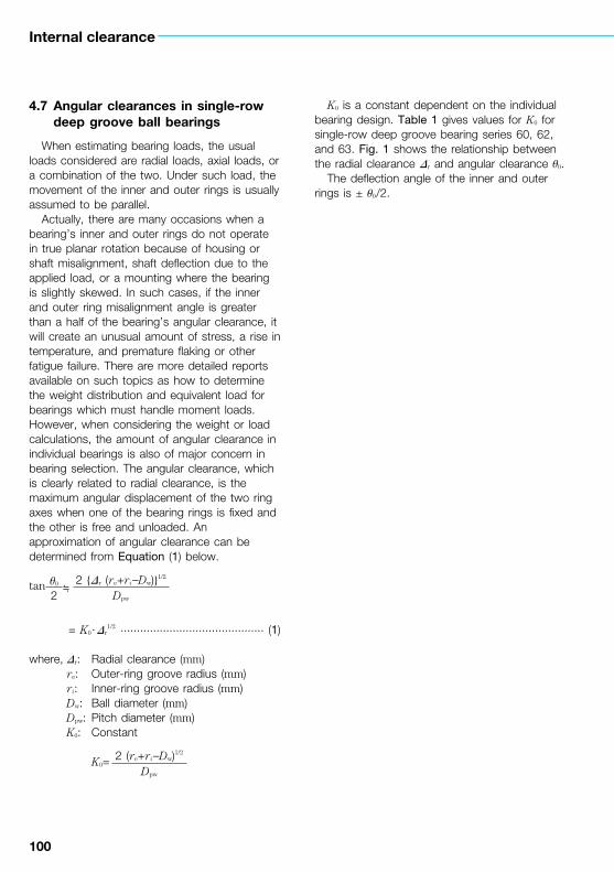
100

Internal clearance

4.7 Angular clearances in single-row deep groove ball bearings

When estimating bearing loads, the usual loads considered are radial loads, axial loads, or a combination of the two. Under such load, the movement of the inner and outer rings is usually assumed to be parallel.

Actually, there are many occasions when a bearing’s inner and outer rings do not operate in true planar rotation because of housing or shaft misalignment, shaft deflection due to the applied load, or a mounting where the bearing is slightly skewed. In such cases, if the inner and outer ring misalignment angle is greater than a half of the bearing’s angular clearance, it will create an unusual amount of stress, a rise in temperature, and premature flaking or other fatigue failure. There are more detailed reports available on such topics as how to determine the weight distribution and equivalent load for bearings which must handle moment loads. However, when considering the weight or load calculations, the amount of angular clearance in individual bearings is also of major concern in bearing selection. The angular clearance, which is clearly related to radial clearance, is the maximum angular displacement of the two ring axes when one of the bearing rings is fixed and the other is free and unloaded. An approximation of angular clearance can be determined from Equation (1) below.

tan ≒

= K0·Dr1/2 ............................................ (1)

where, Dr: Radial clearance (mm) re: Outer-ring groove radius (mm) ri: Inner-ring groove radius (mm) Dw: Ball diameter (mm) Dpw: Pitch diameter (mm) K0: Constant

K0=

K0 is a constant dependent on the individual bearing design. Table 1 gives values for K0 for single-row deep groove bearing series 60, 62, and 63. Fig. 1 shows the relationship between the radial clearance Dr and angular clearance q0.

The deflection angle of the inner and outer rings is ± q0/2.

q0

22 {Dr (re+ri–Dw)}1/2

Dpw

2 (re+ri–Dw)1/2

Dpw

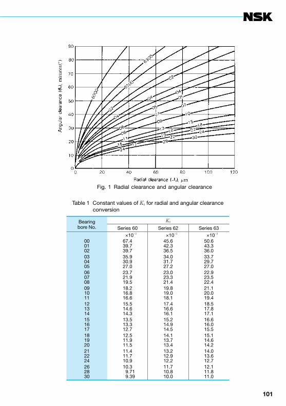
100 101

Fig. 1　Radial clearance and angular clearance

Table 1 Constant values of K0 for radial and angular clearance conversion

Bearingbore No.

K0

Series 60 Series 62 Series 63

000102030405060708091011121314151617181920212224262830

　　　　　×10−3

67.439.739.735.930.927.023.721.919.518.216.816.615.514.614.313.513.312.712.511.911.511.411.710.910.3

9.71 9.39

　　　　　×10−3

45.642.336.534.031.727.223.023.321.419.819.018.117.416.616.115.214.914.514.113.713.413.212.912.211.710.810.0

　　　　　×10−3

50.643.336.033.729.727.022.923.522.421.120.019.418.517.817.116.616.015.515.114.614.214.013.612.712.111.811.0

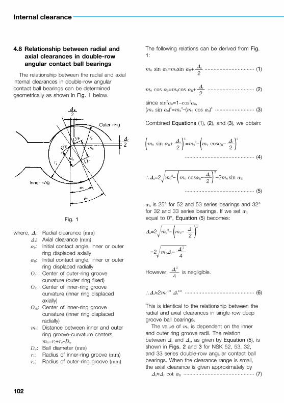
102

Internal clearance

4.8 Relationship between radial and axial clearances in double-row angular contact ball bearings

The relationship between the radial and axial internal clearances in double-row angular contact ball bearings can be determined geometrically as shown in Fig. 1 below.

where, Dr: Radial clearance (mm) Da: Axial clearance (mm) a0: Initial contact angle, inner or outer

ring displaced axially aR: Initial contact angle, inner or outer

ring displaced radially Oe: Center of outer-ring groove

curvature (outer ring fixed) Oi0: Center of inner-ring groove

curvature (inner ring displaced axially)

OiR: Center of inner-ring groove curvature (inner ring displaced radially)

m0: Distance between inner and outer ring groove-curvature centers, m0=ri+re–Dw

Dw: Ball diameter (mm) ri: Radius of inner-ring groove (mm) re: Radius of outer-ring groove (mm)

The following relations can be derived from Fig. 1:

m0 sin a0=m0sin aR+ ................................. (1)

m0 cos a0=m0cos aR+ ............................... (2)

since sin2a0=1–cos2a0,(m0 sin a0)2=m0

2–(m0 cos a0)2 .......................... (3)

Combined Equations (1), (2), and (3), we obtain:

m0 sin aR+ 2

=m02– m0 cosaR–

2

.............................................. (4)

\Da=2 m02– m0 cosaR–

2

–2m0 sin aR

.............................................. (5)

aR is 25° for 52 and 53 series bearings and 32° for 32 and 33 series bearings. If we set aR equal to 0°, Equation (5) becomes:

Da=2 m02– m0–

2

=2 m0Dr–

However, is negligible.

\Da≒2m01/2 Dr

1/2 .............................................. (6)

This is identical to the relationship between the radial and axial clearances in single-row deep groove ball bearings.

The value of m0 is dependent on the inner and outer ring groove radii. The relation between Dr and Da, as given by Equation (5), is shown in Figs. 2 and 3 for NSK 52, 53, 32, and 33 series double-row angular contact ball bearings. When the clearance range is small, the axial clearance is given approximately byDa≒Dr cot aR ............................................... (7)

Da

2

Dr

2

Da

2( ) ( )Dr

2

( )Dr

2

( )Dr

2

Dr2

4

Dr2

4

Fig. 1

102 103

However, when the clearance is relatively large, (when Dr/Dw > 0.002) the error in Equation (7) can be quite large.

The contact angle aR is independent of the

radial clearance; however, the initial contact angle a0 varies with the radial clearance when the inner or outer ring is displaced axially. This relationship is given by Equation (2).

Fig. 2　Radial and axial clearances of bearing series 52 and 53

Fig. 3　Radial and axial clearances of bearing series 32 and 33

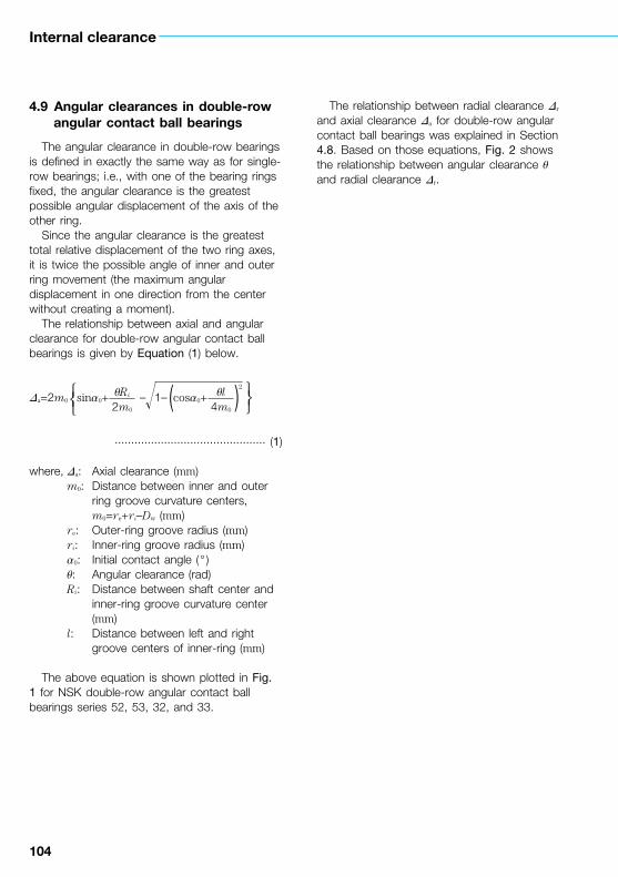
104

Internal clearance

4.9 Angular clearances in double-row angular contact ball bearings

The angular clearance in double-row bearings is defined in exactly the same way as for single-row bearings; i.e., with one of the bearing rings fixed, the angular clearance is the greatest possible angular displacement of the axis of the other ring.

Since the angular clearance is the greatest total relative displacement of the two ring axes, it is twice the possible angle of inner and outer ring movement (the maximum angular displacement in one direction from the center without creating a moment).

The relationship between axial and angular clearance for double-row angular contact ball bearings is given by Equation (1) below.

Da=2m0 sina0+ – 1– cosa0+ 2

.............................................. (1)

where, Da: Axial clearance (mm) m0: Distance between inner and outer

ring groove curvature centers, m0=re+ri–Dw (mm)

re: Outer-ring groove radius (mm) ri: Inner-ring groove radius (mm) a0: Initial contact angle (° ) q: Angular clearance (rad) Ri: Distance between shaft center and

inner-ring groove curvature center (mm)

l: Distance between left and right groove centers of inner-ring (mm)

The above equation is shown plotted in Fig. 1 for NSK double-row angular contact ball bearings series 52, 53, 32, and 33.

The relationship between radial clearance Dr and axial clearance Da for double-row angular contact ball bearings was explained in Section 4.8. Based on those equations, Fig. 2 shows the relationship between angular clearance q and radial clearance Dr.

( )ql4m0

qRi

2m0

104 105

Fig. 1　Relationship between axial and angular clearances

Fig. 2　Relationship between radial and angular clearances

106

Internal clearance

4.10 Measuring method of internal clearance of combined tapered roller bearings (offset measuring method)

Combined tapered roller bearings are available in two types: a back-to-back combination (DB type) and a face-to-face combination (DF type) (see Fig. 1 and Fig. 2). The advantages of these combinations can be obtained by assembly as one set or combined with other bearings to be a fixed- or free-side bearing.

For the DB type of combined tapered roller bearing, as its cage protrudes from the back side of the outer ring, the outer ring spacer (K spacer in Fig. 1) is mounted to prevent mutual contact of cages. For the inner ring, the inner ring spacer (L spacer in Fig. 1), having an appropriate width, is provided to secure the clearance. For the DF type, as shown in Fig. 2, bearings are used with a K spacer.

In general, to use such a bearing arrangement either an appropriate clearance is required that takes into account the heat generated during operation or an applied preload is required that increases the rigidity of the bearings. The spacer width should be adjusted so as to provide an appropriate clearance or preload (minus clearance) after mounting.

Hereunder, we introduce you to a clearance measurement method for a DB arrangement.(1) As shown in Fig. 3, put the bearing A on the surface plate and after stabilization of rollers by rotating the outer ring (more than 10 turns), measure the offset fA=TA–BA.(2) Next, as shown in Fig. 4, use the same procedure to measure the other bearing B for its offset fB=TB–BB.(3) Next, measure the width of the K and L spacers as shown in Fig. 5.

From the results of the above measurements, the axial clearance Da of the combined tapered roller bearing can be obtained, with the use of symbols shown in Figs. 3 through 5 by Equation (1):

Da=(L–K)–( fA+ fB) ......................................... (1)

As an example, for the combined tapered roller bearing HR32232JDB+KLR10AC3, confirm the clearance of the actual product conforms to the specifications. First, refer to NSK Rolling Bearing Catalog CAT. No. E1102 (Page A93) and notice that the C3 clearance range is Dr=110 to 140 mm.To compare this specification with the offset measurement results, convert it into an axial clearance Da by using Equation (2):

Da=Drcot a≒Dr ....................................... (2)

where, e: Constant determined for each bearing No. (Listed in the Bearing Tables of NSK Rolling Bearings Catalog)

refering to the said catalog (Page B127), with use of e=0.44, the following is obtained:

Da=(110 to 140)×

≒380 to 480 mm

It is possible to confirm that the bearing clearance is C3, by verifying that the axial clearance Da of Equation (1) (obtained by the bearing offset measurement) is within the above mentioned range.

1.5e

1.5e

106 107

TA BA

fA

TB BB

fB

Bearing A

Bearing A

Bearing B

Bearing BK spacer L spacer

Bearing A Bearing BK spacer

Fig. 1　DB arrangement Fig. 2　DF arrangement

Fig. 3

Fig. 4

Fig. 5

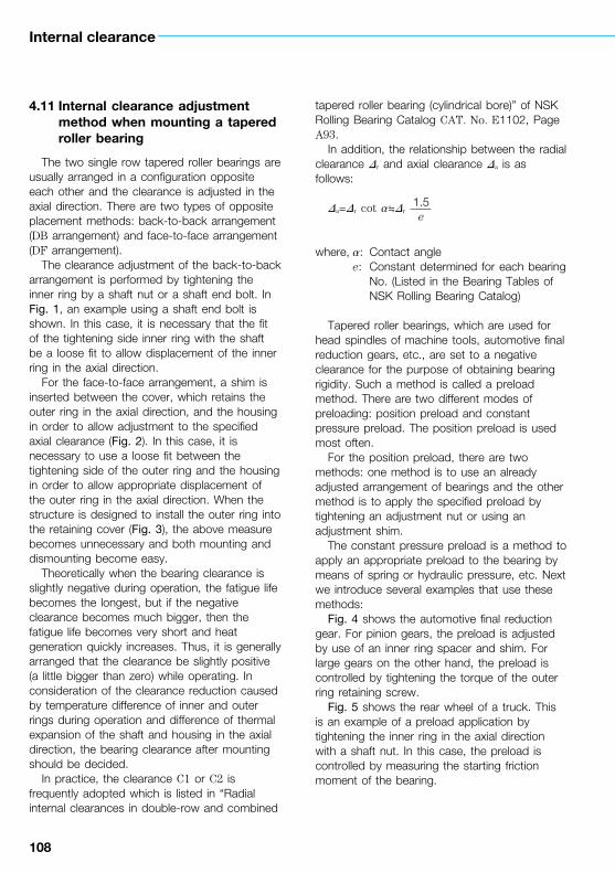
108

Internal clearance

4.11 Internal clearance adjustment method when mounting a tapered roller bearing

The two single row tapered roller bearings are usually arranged in a configuration opposite each other and the clearance is adjusted in the axial direction. There are two types of opposite placement methods: back-to-back arrangement (DB arrangement) and face-to-face arrangement (DF arrangement).

The clearance adjustment of the back-to-back arrangement is performed by tightening the inner ring by a shaft nut or a shaft end bolt. In Fig. 1, an example using a shaft end bolt is shown. In this case, it is necessary that the fit of the tightening side inner ring with the shaft be a loose fit to allow displacement of the inner ring in the axial direction.

For the face-to-face arrangement, a shim is inserted between the cover, which retains the outer ring in the axial direction, and the housing in order to allow adjustment to the specified axial clearance (Fig. 2). In this case, it is necessary to use a loose fit between the tightening side of the outer ring and the housing in order to allow appropriate displacement of the outer ring in the axial direction. When the structure is designed to install the outer ring into the retaining cover (Fig. 3), the above measure becomes unnecessary and both mounting and dismounting become easy.

Theoretically when the bearing clearance is slightly negative during operation, the fatigue life becomes the longest, but if the negative clearance becomes much bigger, then the fatigue life becomes very short and heat generation quickly increases. Thus, it is generally arranged that the clearance be slightly positive (a little bigger than zero) while operating. In consideration of the clearance reduction caused by temperature difference of inner and outer rings during operation and difference of thermal expansion of the shaft and housing in the axial direction, the bearing clearance after mounting should be decided.

In practice, the clearance C1 or C2 is frequently adopted which is listed in “Radial internal clearances in double-row and combined

tapered roller bearing (cylindrical bore)” of NSK Rolling Bearing Catalog CAT. No. E1102, Page A93.

In addition, the relationship between the radial clearance Dr and axial clearance Da is as follows:

Da=Dr cot a≒Dr

where, a: Contact angle e: Constant determined for each bearing

No. (Listed in the Bearing Tables of NSK Rolling Bearing Catalog)

Tapered roller bearings, which are used for head spindles of machine tools, automotive final reduction gears, etc., are set to a negative clearance for the purpose of obtaining bearing rigidity. Such a method is called a preload method. There are two different modes of preloading: position preload and constant pressure preload. The position preload is used most often.

For the position preload, there are two methods: one method is to use an already adjusted arrangement of bearings and the other method is to apply the specified preload by tightening an adjustment nut or using an adjustment shim.

The constant pressure preload is a method to apply an appropriate preload to the bearing by means of spring or hydraulic pressure, etc. Next we introduce several examples that use these methods:

Fig. 4 shows the automotive final reduction gear. For pinion gears, the preload is adjusted by use of an inner ring spacer and shim. For large gears on the other hand, the preload is controlled by tightening the torque of the outer ring retaining screw.

Fig. 5 shows the rear wheel of a truck. This is an example of a preload application by tightening the inner ring in the axial direction with a shaft nut. In this case, the preload is controlled by measuring the starting friction moment of the bearing.

1.5e

108 109

Fig. 6 shows an example of the head spindle of the lathe, the preload is adjusted by tightening the shaft nut.

Fig. 7 shows an example of a constant pressure preload for which the preload is

adjusted by the displacement of the spring. In this case, first find a relationship between the spring’s preload and displacement, then use this information to establish a constant pressure preload.

Fig. 1　DB arrangement whose clearance is adjusted by inner rings.

Fig. 2　DF arrangement whose clearance is adjusted by outer rings.

Fig. 3　Examples of clearance adjusted by shim thickness of outer ring cover

Fig. 4　Automotive final reduction gear

Fig. 5　Rear wheel of truck

Fig. 6　Head spindle of lathe

Fig. 7　Constant pressure preload applied by spring

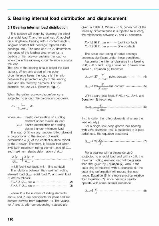
110

5. Bearing internal load distribution and displacement

5.1 Bearing internal load distribution

This section will begin by examing the effect of a radial load Fr and an axial load Fa applied on a single-row bearing with a contact angle a (angular contact ball bearings, tapered roller bearings, etc.). The ratio of Fa to Fr determines the range of the loading area when just a portion of the raceway sustains the load, or when the entire raceway circumference sustains the load.The size of the loading area is called the load factor ε. When only a part of the outer circumference bears the load, ε is the ratio between the projected length of the loading area and the raceway diameter. For this example, we use ε≦1. (Refer to Fig. 1).

When the entire raceway circumference is subjected to a load, the calculation becomes,

ε = ≧1

where, dmax: Elastic deformation of a rolling element under maximum load

dmin: Elastic deformation of a rolling element under minimum load

The load Q (y) on any random rolling element is proportional to the amount of elastic deformation d (y) of the contact surface raised to the t power. Therefore, it follows that when y=0 (with maximum rolling element load of Qmax and maximum elastic deformation of dmax),

= t

....................................... (1)

t=1.5 (point contact), t=1.1 (line contact)The relations between the maximum rolling

element load Qmax, radial load Fr, and axial load Fa are as follows:

Fr=Jr Z Qmax cos a ...................................... (2)Fa=Ja Z Qmax sin a ...................................... (3)

where Z is the number of rolling elements, and Jr and Ja are coefficients for point and line contact derived from Equation (1). The values for Jr and Ja with corresponding ε values are

given in Table 1. When ε =0.5, (when half of the raceway circumference is subjected to a load), the relationship between Fa and Fr becomes,

Fa=1.216 Fr tan a ........ (point contact)Fa=1.260 Fr tan a ........ (line contact)

The basic load rating of radial bearings becomes significant under these conditions.

Assuming the internal clearance in a bearing D=0, ε =0.5 and using a value for Jr taken from Table 1, Equation (2) becomes,

Qmax=4.37 point contact ................. (4)

Qmax=4.08 line contact ................... (5)

With a pure axial load, Fr=0, ε =∞, Ja=1, and Equation (3) becomes;

Q=Qmax= ......................................... (6)

(In this case, the rolling elements all share the load equally.)

For a single-row deep groove ball bearing with zero clearance that is subjected to a pure radial load, the equation becomes;

Qmax=4.37 .............................................. (7)

For a bearing with a clearance D >0 subjected to a radial load and with ε <0.5, the maximum rolling element load will be greater than that given by Equation (7). Also, if the outer ring is mounted with a clearance fit, the outer ring deformation will reduce the load range. Equation (8) is a more practical relation than Equation (7), since bearings usually operate with some internal clearance.

Qmax=5 ................................................... (8)

dmax

dmax– dmin

Q (y)

Qmax

d (y)

dmax( )

Fr

Z cosa

Fr

Z cosa

Fa

Z sina

Fr

Z

Fr

Z

110 111

Fig. 1

Table 1 Values for Jr and Ja in single-row bearings

εPoint contact Line contact

Frtan a────Fa

Jr JaFrtan a────

Fa

Jr Ja

00.10.2

0.30.40.5

0.60.70.8

0.91.01.25

1.672.55

∞

10.96630.9318

0.89640.86010.8225

0.78350.74270.6995

0.65290.60000.4338

0.30880.18500.08310

00.11560.1590

0.18920.21170.2288

0.24160.25050.2559

0.25760.25460.2289

0.18710.13390.07110

00.11960.1707

0.21100.24620.2782

0.30840.33740.3658

0.39450.42440.5044

0.60600.72400.85581

10.96130.9215

0.88050.83800.7939

0.74800.69990.6486

0.59200.52380.3598

0.23400.13720.06110

00.12680.1737

0.20550.22860.2453

0.25680.26360.2658

0.26280.25230.2078

0.15890.10750.05440

00.13190.1885

0.23340.27280.3090

0.34330.37660.4098

0.44390.48170.5775

0.67900.78370.89091

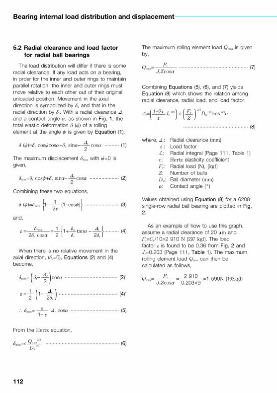
112

Bearing internal load distribution and displacement

5.2 Radial clearance and load factor for radial ball bearings

The load distribution will differ if there is some radial clearance. If any load acts on a bearing, in order for the inner and outer rings to maintain parallel rotation, the inner and outer rings must move relative to each other out of their original unloaded position. Movement in the axial direction is symbolized by da and that in the radial direction by dr. With a radial clearance Dr and a contact angle a, as shown in Fig. 1, the total elastic deformation d (y) of a rolling element at the angle y is given by Equation (1).

d (y)=dr cosycosa+da sina– cosa .......... (1)

The maximum displacement dmax with y=0 is given,

dmax=dr cosy+da sina– cosa .................... (2)

Combining these two equations,

d (y)=dmax 1– (1–cosy) ....................... (3)

and,

ε = = 1+ tana – .......... (4)

When there is no relative movement in the axial direction, (da=0), Equations (2) and (4) become,

dmax= dr– cosa .................................... (2)’

ε = 1– ........................................ (4)’

\ dmax= Dr cosa ................................. (5)

From the Hertz equation,

dmax=c .................................................. (6)

The maximum rolling element load Qmax is given by,

Qmax= ............................................... (7)

Combining Equations (5), (6), and (7) yields Equation (8) which shows the relation among radial clearance, radial load, and load factor.

Dr= Jr–2/3 c

2/3

Dw–1/3cos–5/3a

............................................ (8)

where, Dr: Radial clearance (mm) ε : Load factor Jr: Radial integral (Page 111, Table 1) c: Hertz elasticity coefficient Fr: Radial load (N), {kgf} Z: Number of balls Dw: Ball diameter (mm) a: Contact angle (° )

Values obtained using Equation (8) for a 6208 single-row radial ball bearing are plotted in Fig. 2.

As an example of how to use this graph, assume a radial clearance of 20 mm and Fr=Cr/10=2 910 N {297 kgf}. The load factor ε is found to be 0.36 from Fig. 2 and Jr=0.203 (Page 111, Table 1). The maximum rolling element load Qmax can then be calculated as follows,

Qmax= = =1 590N {163kgf}

Dr

2

Dr

2

12 ε

dmax

2dr cosa12

da

dr

Dr

2dr

Dr

2( )12

Dr

2dr( )

ε1– ε

Qmax2/3

Dw1/3

Fr

JrZcosa

1–2 εε

Fr

Z( ) ( )

Fr

JrZcosa2 910

0.203×9

112 113

Fig. 1

Fig. 2

114


5.3 Radial clearance and maximum rolling element load

If we consider an example where a deep groove ball bearing is subjected to a radial load and the radial clearance Dr is 0, then the load factor ε will be 0.5. When Dr>0 (where there is a clearance), ε <0.5; when Dr<0, ε >0.5. (See Fig. 1).

Fig. 2 in section 5.2 shows how the load factor change due to clearance decreases with increasing radial load.

When the relationship between radial clearance and load factor is determined, it can be used to establish the relationship between radial clearance and bearing life, and between radial clearance and maximum rolling element load.

The maximum rolling element load is calculated using Equation (1).

Qmax= ............................................. (1)

where, Fr: Radial load (N), {kgf} Jr: Radial integral Z: Number of balls a: Contact angle (° )

Jr is dependent on the value of ε (Page 111, Table 1), and ε is determined, as explained in Section 5.2, from the radial load and radial clearance.

Fig. 2 shows the relationship between the radial clearance and maximum rolling element load for a 6208 deep groove ball bearing. As can be seen from Fig. 2, the maximum rolling element load increases with increasing radial clearance or reduction in the loaded range. When the radial clearance falls slightly below zero, the loaded range grows widely resulting in minimum in the maximum rolling element load. However, as the compression load on all rolling elements is increased when the clearance is further reduced, the maximum rolling element load begins to increase sharply.Fr

JrZcosa

Fig. 1　Radial clearance and load distribution

114 115

Fig. 2　Radial clearance and maximum rolling element load

116


5.4 Contact surface pressure and contact ellipse of ball bearings under pure radial loads

Details about the contact between a rolling element and raceway is a classic exercise in the Hertz theory and one where theory and practice have proven to agree well. It also forms the basis for theories on ball bearing life and friction.

Generally, the contact conditions between the inner ring raceway and ball is more severe than those between the outer ring raceway and ball. Moreover, when checking the running trace (rolling contact trace), it is much easier to observe the inner ring raceway than the outer ring raceway. Therefore, we explain the relation of contact ellipse width and load between an inner ring raceway and a ball in a deep groove ball bearing. With no applied load, the ball and inner ring raceway meet at a point. When a load is applied to the bearing, however, elastic deformation is caused and the contact area assumes an elliptical shape as shown in Fig. 1.

When a ball bearing is subjected to a load, the resulting maximum contact surface pressure on the elliptical area of contact between a ball and a bearing raceway is Pmax. The major axis of the ellipse is represented by 2a and the minor axis by 2b. The following relationships were derived from the Hertz equation.

Pmax= 1– –2/3

(Sr)2/3Q1/3

= (Sr)2/3Q1/3

(MPa), {kgf/mm2} ................... (1)

where, Constant A1: 858 for (N-unit), 187 for {kgf-unit}

2a=m 1/3

=A2m 1/3

(mm) ................................. (2)

where, Constant A2 : 0.0472 for (N-unit), 0.101 for {kgf-unit}

2b=ν 1/3

=A2ν 1/3

(mm) .................................. (3)

where, E : Young’s modulus (Steel: E=208 000 MPa {21 200 kgf/mm2})

m : Poisson’s number (Steel: 10/3) Q : Rolling element (ball) load (N), {kgf} Sr : Total major curvatureFor radial ball bearing,

Sr= 4– ± ................................. (4)

Symbol of ± : The upper is for inner ring. The lower is for outer ring.

Dw : Ball diameter (mm)f : Ratio of groove radius to ball

diameterg : Dwcosa/Dpw

Dpw : Ball pitch diameter (mm)a : Contact angle (° )

m and ν are shown in Fig. 2 based on cost in Equation (5).

±cos t= ................................... (5) 4– ±

Symbol of ± : The upper is for the inner ring. The lower is for the outer ring.

If the maximum rolling element load of the ball bearing under the radial load Fr is Qmax and the number of balls is Z, an approximate relation between them is shown in Equation (6).

Qmax=5 ........................................................ (6)

1.5p

3E

1m2

1mν( )

A1

mν

24 ( 1– 1m2 ) Q

ESr

QSr( )

24 (1– 1m2 ) Q

ESr

QSr( )

1Dw

1f( )

1f

Fr

Z

2g1 g±

1f

2g1 g±

2g1 g±

116 117

2a

2b Contact ellipse

Running trace

Fig. 1　Inner ring raceway running trace (Rolling contact trace)

Fig. 2　m and ν values against cost

118


Therefore, Equations (1), (2), and (3) can be changed into the following equations by substituting Equations (4) and (6).

Pmax =K1·Fr1/3 (MPa) ............. (7)

=0.218K1·Fr1/3 {kgf/mm2}

2a =K2·Fr1/3 (N)

(mm) ........... (8)

=2.14K2·Fr1/3 {kgf}

2b =K3·Fr1/3 (N)

(mm) ............ (9)

=2.14K3·Fr1/3 {kgf}

Table 1 gives values for the constants K1, K2,, and K3 for different bearing numbers.

Generally, the ball bearing raceway has a running trace caused by the balls whose width is equivalent to 2a. We can estimate the applied load by referring to the trace on the raceway. Therefore, we can judge whether or not any abnormal load was sustained by the bearing which was beyond what the bearing was originally designed to carry.

ExampleThe pure radial load, Fr=3 500 N (10% of basic dynamic load rating), is applied to a deep groove ball bearing, 6210. Calculate the maximum surface pressure, Pmax, and contact widths of the ball and inner ring raceway, 2a and 2b.

Using the figures of K1 ~ K3 in Table 1, the following values can be obtained.

Pmax = K1·Fr1/3=143×3 5001/3=2 170 (MPa)

2a = K2·Fr1/3=0.258×3 5001/3=3.92 (mm)

2b = K3·Fr1/3=0.026×3 5001/3=0.39 (mm)

Bearingbore No.

Bearing series 60

K1 K2 K3

000102

030405

060708

091011

121314

151617

181920

212224

262830

324305287

274191181

160148182

166161148

144140130

127120117

111108108

10298.295.3

88.185.981.8

0.2150.2050.196

0.1890.3320.320

0.3260.3420.205

0.2060.2010.219

0.2140.2090.224

0.2190.2350.229

0.2440.2380.238

0.2430.2680.261

0.2630.2570.264

0.0200.0190.019

0.0180.0170.016

0.0170.0170.021

0.0210.0210.023

0.0220.0220.023

0.0230.0240.024

0.0250.0250.025

0.0260.0280.027

0.0280.0270.028

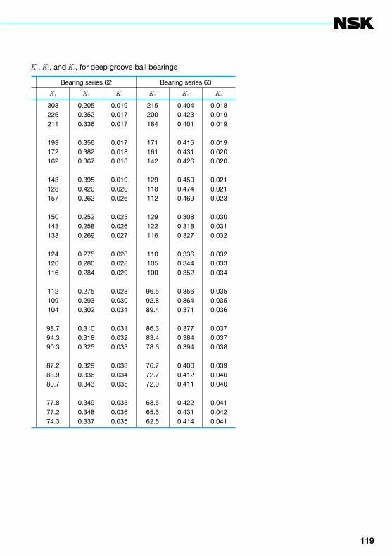
118 119

K1, K2, and K3, for deep groove ball bearings

Bearing series 62 Bearing series 63

K1 K2 K3 K1 K2 K3

303226211

193172162

143128157

150143133

124120116

112109104

98.794.390.3

87.283.980.7

77.877.274.3

0.2050.3520.336

0.3560.3820.367

0.3950.4200.262

0.2520.2580.269

0.2750.2800.284

0.2750.2930.302

0.3100.3180.325

0.3290.3360.343

0.3490.3480.337

0.0190.0170.017

0.0170.0180.018

0.0190.0200.026

0.0250.0260.027

0.0280.0280.029

0.0280.0300.031

0.0310.0320.033

0.0330.0340.035

0.0350.0360.035

215200184

171161142

129118112

129122116

110105100

96.592.889.4

86.383.478.6

76.772.772.0

68.565.562.5

0.4040.4230.401

0.4150.4310.426

0.4500.4740.469

0.3080.3180.327

0.3360.3440.352

0.3560.3640.371

0.3770.3840.394

0.4000.4120.411

0.4220.4310.414

0.0180.0190.019

0.0190.0200.020

0.0210.0210.023

0.0300.0310.032

0.0320.0330.034

0.0350.0350.036

0.0370.0370.038

0.0390.0400.040

0.0410.0420.041

120


5.5 Contact surface pressure and contact area under pure radial load (roller bearings)

The following equations, Equations 1 and 2, which were derived from the Hertz equation, give the contact surface pressure Pmax between two axially-parallel cylinders and the contact area width 2b (Fig. 1).

Pmax= =A1

(MPa) {kgf/mm2} .................... (1)

where, constant A1: 191 .................... (N-unit): 60.9 ................ {kgf-unit}

2b= =A2

(mm) ..................................... (2)

where, constant A2: 0.00668 ................. (N-unit): 0.0209 ................ {kgf-unit}

where, E: Young’s modulus (Steel: E=208 000 MPa {21 200 kgf/mm2})

m: Poisson’s number (for steel, m=10/3)

Sr: Composite curvature for both cylinders

Sr=rI1+rII1 (mm–1) rI1: Curvature, cylinier I (roller) rI1=1/Dw/2=2/Dw (mm–1) rII1: Curvature, cylinier II (raceway) rII1=1/Di/2=2/Di (mm–1) for inner ring

raceway rII1=−1/De/2=−2/De (mm–1) for outer

ring raceway Q: Normal load on cylinders (N), {kgf} Lwe: Effective contact length of cylinders

(mm)

When a radial load Fr is applied on a radial roller bearing, the maximum rolling element load Qmax for practical use is given by Equation (3).

Qmax= (N), {kgf} ........................ (3)

where, i: Number of roller rows Z: Number of rollers per row a: Contact angle (° )

The contact surface pressure Pmax and contact width 2b of raceway and roller which sustains the largest load are given by Equations (4) and (5).

Pmax = K1 √—Fr (MPa) ............. (4) = 0.319K1 √—Fr {kgf/mm2}

2b = K2 √—Fr (N) .................. (5) = 3.13K2 √—Fr {kgf}

The constant K1 and K2 of cylindrical roller bearings and tapered roller bearings are listed in Tables 1 to 6 according to the bearing numbers. K1i and K2i are the constants for the contact of roller and inner ring raceway, and K1e and K2e are the constants for the contact of roller and outer ring raceway.

E · Sr ·Q

2p (1– 1m2

) Lwe

Sr ·QLw

32 (1– 1m2 ) Q

p ·E · Sr ·Lw

QSr ·Lw

4.6 Fr

i Zcosa

120 121

ExampleA pure radial load, Fr=4 800 N (10% of basic

dynamic load rating), is applied to the cylindrical roller bearing, NU210. Calculate the maximum surface pressure, Pmax, and contact widths of the roller and raceway, 2b.

Using the figures of K1i, K1e K2i, and K2e in Table 1, the following values can be obtained.

Contact of roller and inner ring raceway:Pmax=K1i √—Fr=17.0× 4 800=1 180 (MPa)2b=K2i √—Fr=2.55×10–3× 4 800=0.18 (mm)

Contact of roller and outer ring raceway:Pmax=K1e √—Fr=14.7× 4 800=1 020 (MPa)2b=K2e √—Fr=2.95×10–3× 4 800=0.20 (mm)

√———

√———

√———

√———

Fig. 1　Contact surface pressure Pmax and contact width 2b

122


Table 1 Constants, K1i, K1e, K2i, and K2e, for cylindrical roller bearings

BearingNo.

Bearing series NU2 BearingNo.

Bearing series NU3

K1i K1e K2i K2e K1i K1e K2i K2e

NU205WNU206WNU207W

NU208WNU209WNU210W

NU211WNU212WNU213W

NU214WNU215WNU216W

NU217WNU218WNU219W

NU220WNU221WNU222W

NU224WNU226WNU228WNU230W

30.626.121.6

18.517.717.0

15.414.012.5

12.411.511.0

10.29.108.98

8.237.827.36

7.026.766.275.80

25.822.218.2

15.715.214.7

13.312.210.8

10.910.19.57

8.947.877.77

7.136.786.34

6.085.915.485.07

2.902.872.83

2.702.632.55

2.542.532.44

2.452.442.49

2.482.452.56

2.472.472.53

2.532.462.472.47

3.443.393.36

3.203.072.95

2.932.922.82

2.812.802.86

2.852.842.96

2.852.852.93

2.922.822.832.83

NU305WNU306WNU307W

NU308WNU309WNU310W

NU311WNU312WNU313W

NU314WNU315WNU316W

NU317WNU318WNU319W

NU320WNU321WNU322W


24.220.517.7

16.114.413.1

11.510.810.3

9.358.838.43

8.047.457.14

6.616.426.06

5.385.074.804.61

19.616.814.6

13.411.810.8

9.448.918.54

7.787.317.05

6.686.225.97

5.525.345.04

4.444.213.993.85

3.032.892.76

2.762.852.79

2.762.762.79

2.682.772.68

2.762.682.68

2.662.762.78

2.752.752.752.79

3.733.523.35

3.323.463.37

3.363.343.37

3.223.343.20

3.323.213.20

3.193.313.34

3.333.323.313.34

─×10−3──×10−3 ─×10−3──×10−3

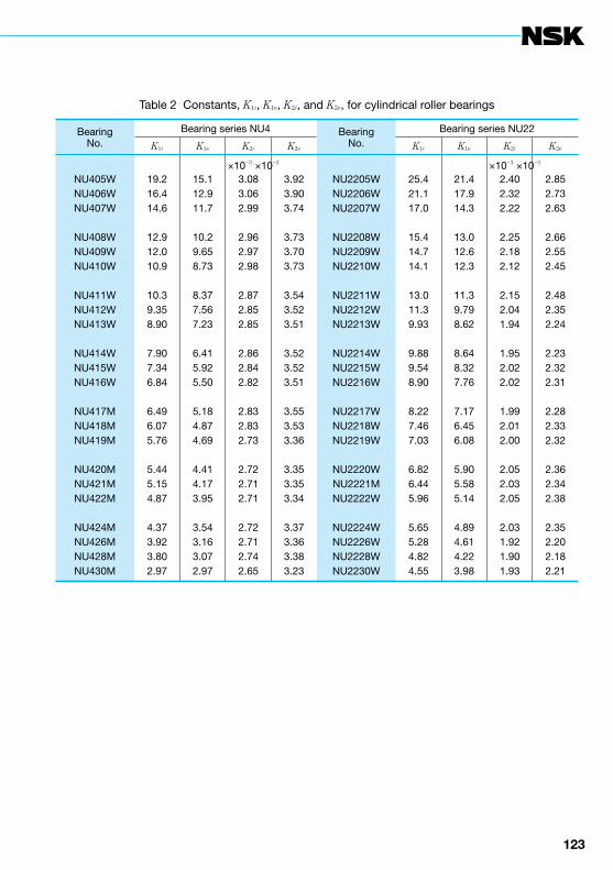
122 123


BearingNo.


Bearing series NU22


NU405WNU406WNU407W

NU408WNU409WNU410W

NU411WNU412WNU413W

NU414WNU415WNU416W

NU417MNU418MNU419M

NU420MNU421MNU422M

NU424MNU426MNU428MNU430M

19.216.414.6

12.912.010.9

10.39.358.90

7.907.346.84

6.496.075.76

5.445.154.87

4.373.923.802.97

15.112.911.7

10.29.658.73

8.377.567.23

6.415.925.50

5.184.874.69

4.414.173.95

3.543.163.072.97

3.083.062.99

2.962.972.98

2.872.852.85

2.862.842.82

2.832.832.73

2.722.712.71

2.722.712.742.65

3.923.903.74

3.733.703.73

3.543.523.51

3.523.523.51

3.553.533.36

3.353.353.34

3.373.363.383.23

NU2205WNU2206WNU2207W





NU2220WNU2221MNU2222W


25.421.117.0

15.414.714.1

13.011.39.93

9.889.548.90

8.227.467.03

6.826.445.96

5.655.284.824.55

21.417.914.3

13.012.612.3

11.39.798.62

8.648.327.76

7.176.456.08

5.905.585.14

4.894.614.223.98

2.402.322.22

2.252.182.12

2.152.041.94

1.952.022.02

1.992.012.00

2.052.032.05

2.031.921.901.93

2.852.732.63

2.662.552.45

2.482.352.24

2.232.322.31

2.282.332.32

2.362.342.38

2.352.202.182.21

─×10−3──×10−3 ─×10−3──×10−3

124



BearingNo.


Bearing series NN30







NU2320WNU2321MNU2322M


19.017.015.6

12.911.910.6

9.538.858.32

7.506.986.66

6.216.115.65

5.404.804.48

4.003.623.433.24

15.414.012.9

10.79.798.76

7.837.316.90

6.245.785.58

5.175.104.73

4.513.993.73

3.313.002.862.70

2.382.412.43

2.222.362.26

2.292.262.26

2.152.192.11

2.142.202.12

2.182.062.05

2.051.961.971.96

2.932.932.96

2.672.862.73

2.782.742.72

2.582.642.53

2.572.632.53

2.602.482.47

2.482.372.362.34

NN3005NN3006NN3007T

NN3008TNN3009TNN3010T





NN3024TNN3026TNN3028NN3030

31.328.124.3

23.120.720.1

17.516.715.9

14.414.012.6

12.311.411.1

10.99.759.04

8.667.867.557.08

27.324.721.5

20.418.418.1

15.615.014.5

13.012.811.4

11.210.310.2

10.08.848.18

7.907.146.906.47

2.362.362.24

2.312.252.20

2.182.092.02

2.042.011.99

1.961.981.95

1.922.002.00

1.931.991.921.92

2.722.692.53

2.612.522.45

2.432.322.22

2.252.202.19

2.152.182.14

2.092.212.20

2.112.192.112.10

─×10−3──×10−3 ─×10−3──×10−3

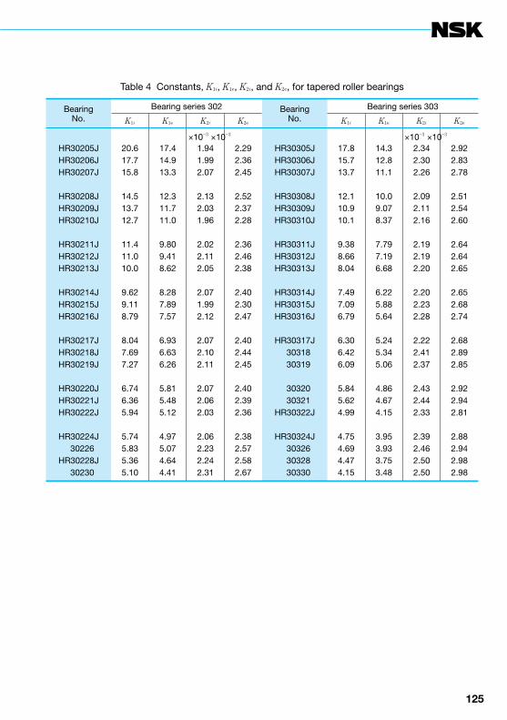
124 125

Table 4 Constants, K1i, K1e, K2i, and K2e, for tapered roller bearings

BearingNo.

Bearing series 302 BearingNo.

Bearing series 303


HR30205JHR30206JHR30207J

HR30208JHR30209JHR30210J

HR30211JHR30212JHR30213J

HR30214JHR30215JHR30216J

HR30217JHR30218JHR30219J

HR30220JHR30221JHR30222J

HR30224J 30226HR30228J 30230

20.617.715.8

14.513.712.7

11.411.010.0

9.629.118.79

8.047.697.27

6.746.365.94

5.745.835.365.10

17.414.913.3

12.311.711.0

9.809.418.62

8.287.897.57

6.936.636.26

5.815.485.12

4.975.074.644.41

1.941.992.07

2.132.031.96

2.022.112.05

2.071.992.12

2.072.102.11

2.072.062.03

2.062.232.242.31

2.292.362.45

2.522.372.28

2.362.462.38

2.402.302.47

2.402.442.45

2.402.392.36

2.382.572.582.67

HR30305JHR30306JHR30307J

HR30308JHR30309JHR30310J

HR30311JHR30312JHR30313J

HR30314JHR30315JHR30316J

HR30317J 30318 30319

30320 30321HR30322J

HR30324J 30326 30328 30330

17.815.713.7

12.110.910.1

9.388.668.04

7.497.096.79

6.306.426.09

5.845.624.99

4.754.694.474.15

14.312.811.1

10.09.078.37

7.797.196.68

6.225.885.64

5.245.345.06

4.864.674.15

3.953.933.753.48

2.342.302.26

2.092.112.16

2.192.192.20

2.202.232.28

2.222.412.37

2.432.442.33

2.392.462.502.50

2.922.832.78

2.512.542.60

2.642.642.65

2.652.682.74

2.682.892.85

2.922.942.81

2.882.942.982.98

─×10−3──×10−3 ─×10−3──×10−3

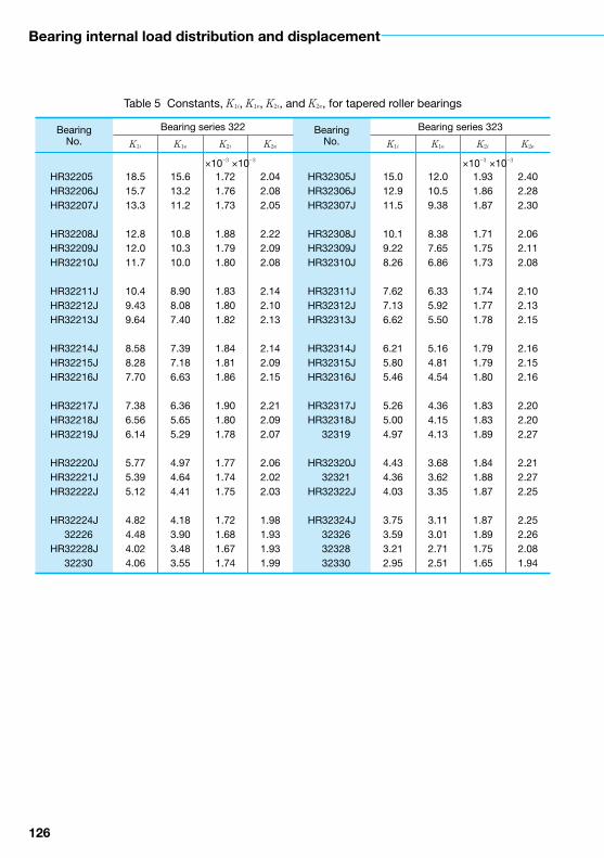
126



BearingNo.

Bearing series 322 BearingNo.

Bearing series 323


HR32205HR32206JHR32207J

HR32208JHR32209JHR32210J

HR32211JHR32212JHR32213J

HR32214JHR32215JHR32216J

HR32217JHR32218JHR32219J

HR32220JHR32221JHR32222J

HR32224J 32226HR32228J 32230

18.515.713.3

12.812.011.7

10.49.439.64

8.588.287.70

7.386.566.14

5.775.395.12

4.824.484.024.06

15.613.211.2

10.810.310.0

8.908.087.40

7.397.186.63

6.365.655.29

4.974.644.41

4.183.903.483.55

1.721.761.73

1.881.791.80

1.831.801.82

1.841.811.86

1.901.801.78

1.771.741.75

1.721.681.671.74

2.042.082.05

2.222.092.08

2.142.102.13

2.142.092.15

2.212.092.07

2.062.022.03

1.981.931.931.99

HR32305JHR32306JHR32307J

HR32308JHR32309JHR32310J

HR32311JHR32312JHR32313J

HR32314JHR32315JHR32316J

HR32317JHR32318J 32319

HR32320J 32321HR32322J

HR32324J 32326 32328 32330

15.012.911.5

10.19.228.26

7.627.136.62

6.215.805.46

5.265.004.97

4.434.364.03

3.753.593.212.95

12.010.59.38

8.387.656.86

6.335.925.50

5.164.814.54

4.364.154.13

3.683.623.35

3.113.012.712.51

1.931.861.87

1.711.751.73

1.741.771.78

1.791.791.80

1.831.831.89

1.841.881.87

1.871.891.751.65

2.402.282.30

2.062.112.08

2.102.132.15

2.162.152.16

2.202.202.27

2.212.272.25

2.252.262.081.94

─×10−3──×10−3 ─×10−3──×10−3

126 127


BearingNo.

Bearing series 303D BearingNo.

Bearing series 320


30305D 30306D

HR30307DJ

HR30308DJHR30309DJHR30310DJ




───

────

22.019.014.8

13.011.910.8

10.09.338.66

8.207.837.37

6.936.966.34

───

────

18.415.812.4

10.89.949.02

8.377.797.23

6.856.546.15

5.795.815.30

───

────

2.422.482.18

2.182.222.21

2.222.262.27

2.282.342.33

2.342.482.37

───

────

2.912.982.62

2.612.662.65

2.662.712.71

2.742.802.80

2.802.982.84

───

────

HR32005XJHR32006XJHR32007XJ






HR32024XJHR32026XJHR32028XJHR32030XJ

21.118.216.4

14.413.313.0

11.310.810.6

9.689.328.15

8.007.367.22

7.106.616.19

6.105.265.154.77

18.415.914.4

12.711.811.6

10.09.699.57

8.708.437.35

7.256.646.54

6.455.995.59

5.524.744.674.32

1.581.611.57

1.481.471.45

1.461.411.39

1.441.391.36

1.341.371.35

1.341.361.39

1.421.411.391.38

1.821.851.79

1.671.651.62

1.641.571.54

1.601.541.51

1.481.521.50

1.471.501.54

1.561.571.541.53

─×10−3──×10−3 ─×10−3──×10−3

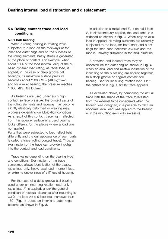
128


5.6 Rolling contact trace and load conditions

5.6.1 Ball bearingWhen a rolling bearing is rotating while

subjected to a load on the raceways of the inner and outer rings and on the surfaces of the rolling elements, heavy stress is generated at the place of contact. For example, when about 10% of the load (normal load) of the Cr, basic dynamic load rating, as radial load, is applied, in the case of deep groove ball bearings, its maximum surface pressure becomes about 2 000 MPa {204 kgf/mm2} and for a roller bearing, the pressure reaches 1 000 MPa {102 kgf/mm2}.

As bearings are used under such high contact surface pressure, the contact parts of the rolling elements and raceway may become slightly elastically deformed or wearing may progress depending on lubrication conditions. As a result of this contact trace, light reflected from the raceway surface of a used bearing looks different for the places where a load was not applied.Parts that were subjected to load reflect light differently and the dull appearance of such parts is called a trace (rolling contact trace). Thus, an examination of the trace can provide insights into the contact and load conditions.

Trace varies depending on the bearing type and conditions. Examination of the trace sometimes allows identification of the cause: radial load only, heavy axial load, moment load, or extreme unevenness of stiffness of housing.

For the case of a deep groove ball bearing used under an inner ring rotation load, only radial load Fr is applied, under the general condition of residual clearance after mounting is Df>0, the load zone y becomes narrower than 180° (Fig. 1), traces on inner and outer rings become as shown in Fig. 2.

In addition to a radial load Fr, if an axial load Fa is simultaneously applied, the load zone y is widened as shown in Fig. 3. When only an axial load is applied, all rolling elements are uniformly subjected to the load, for both inner and outer rings the load zone becomes y=360° and the race is unevenly displaced in the axial direction.

A deviated and inclined trace may be observed on the outer ring as shown in Fig. 4, when an axial load and relative inclination of the inner ring to the outer ring are applied together to a deep groove or angular contact ball bearing used for inner ring rotation load. Or if the deflection is big, a similar trace appears.

As explained above, by comparing the actual trace with the shape of the trace forecasted from the external force considered when the bearing was designed, it is possible to tell if an abnormal axial load was applied to the bearing or if the mounting error was excessive.

128 129

Fig. 1　Load zone under a radial load only

Fig. 3　Load zone for radial load + axial load

2a

2b

Major axis

Min

or a

xis

Contactellipse

Runningtrace

Inner ring

Fig. 2　Trace (rolling contact trace) on raceway surface

Fig. 4　Deviation and inclination of trace (rolling contact trace) on raceway surface of outer ring

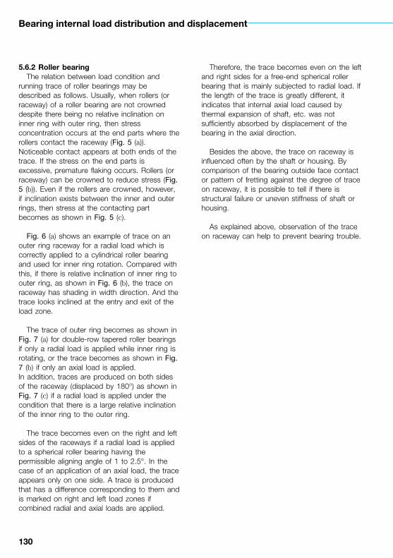
130


5.6.2 Roller bearingThe relation between load condition and

running trace of roller bearings may be described as follows. Usually, when rollers (or raceway) of a roller bearing are not crowned despite there being no relative inclination on inner ring with outer ring, then stress concentration occurs at the end parts where the rollers contact the raceway (Fig. 5 (a)). Noticeable contact appears at both ends of the trace. If the stress on the end parts is excessive, premature flaking occurs. Rollers (or raceway) can be crowned to reduce stress (Fig. 5 (b)). Even if the rollers are crowned, however, if inclination exists between the inner and outer rings, then stress at the contacting part becomes as shown in Fig. 5 (c).

Fig. 6 (a) shows an example of trace on an outer ring raceway for a radial load which is correctly applied to a cylindrical roller bearing and used for inner ring rotation. Compared with this, if there is relative inclination of inner ring to outer ring, as shown in Fig. 6 (b), the trace on raceway has shading in width direction. And the trace looks inclined at the entry and exit of the load zone.

The trace of outer ring becomes as shown in Fig. 7 (a) for double-row tapered roller bearings if only a radial load is applied while inner ring is rotating, or the trace becomes as shown in Fig. 7 (b) if only an axial load is applied.In addition, traces are produced on both sides of the raceway (displaced by 180°) as shown in Fig. 7 (c) if a radial load is applied under the condition that there is a large relative inclination of the inner ring to the outer ring.

The trace becomes even on the right and left sides of the raceways if a radial load is applied to a spherical roller bearing having the permissible aligning angle of 1 to 2.5°. In the case of an application of an axial load, the trace appears only on one side. A trace is produced that has a difference corresponding to them and is marked on right and left load zones if combined radial and axial loads are applied.

Therefore, the trace becomes even on the left and right sides for a free-end spherical roller bearing that is mainly subjected to radial load. If the length of the trace is greatly different, it indicates that internal axial load caused by thermal expansion of shaft, etc. was not sufficiently absorbed by displacement of the bearing in the axial direction.

Besides the above, the trace on raceway is influenced often by the shaft or housing. By comparison of the bearing outside face contact or pattern of fretting against the degree of trace on raceway, it is possible to tell if there is structural failure or uneven stiffness of shaft or housing.

As explained above, observation of the trace on raceway can help to prevent bearing trouble.

130 131

Fig. 5　Stress distribution of cylindrical roller

Fig. 6　Trace (rolling contact trace) of outer ring of cylindrical roller bearing

Fig. 7　Trace (rolling contact trace) of outer ring of double row tapered roller bearing

132


5.7 Radial load and displacement of cylindrical roller bearings

One of the most important requirements for bearings to be used in machine-tool applications is that there be as little deflection as possible with applied loading, i.e. that the bearings have high rigidity.

Double-row cylindrical roller bearings are considered to be the most rigid types under radial loads and also best for use at high speeds. NN30K and NNU49K series are the particular radial bearings most often used in machine tool head spindles.

The amount of bearing displacement under a radial load will vary with the amount of internal clearance in the bearings. However, since machine-tool spindle cylindrical roller bearings are adjusted so the internal clearance after mounting is less than several micrometers, we can consider the internal clearance to be zero for most general calculations. The radial elastic displacement dr of cylindrical roller bearings can be calculated using Equation (1).

dr=0.000077 (N)

(mm) ......... (1)

=0.0006 {kgf}

where, Qmax: Maximum rolling element load (N), {kgf}

Lwe: Effective contact length of roller (mm)

If the internal clearance is zero, the relationship between maximum rolling element load Qmax and radial load Fr becomes: Qmax= Fr (N), {kgf} .......................... (2)

where, i: Number of rows of rollers in a bearing (double-row bearings: i=2)

Z: Number of rollers per row Fr: Radial load (N), {kgf}

Combining Equations (1) and (2), it follows that the relation between radial load Fr and radial displacement dr becomes.

dr=K Fr0.9 (N)

(mm) ........ (3)

=7.8K Fr0.9 {kgf}

where, K=

K is a constant determined by the individual double-row cylindrical roller bearing. Table 1 gives values for K for bearing series NN30. Fig. 1 shows the relation between radial load Fr and radial displacement dr.

Qmax0.9

Lwe0.8

Qmax0.9

Lwe0.8

4.08iZ

0.000146Z 0.9 Lwe

0.8

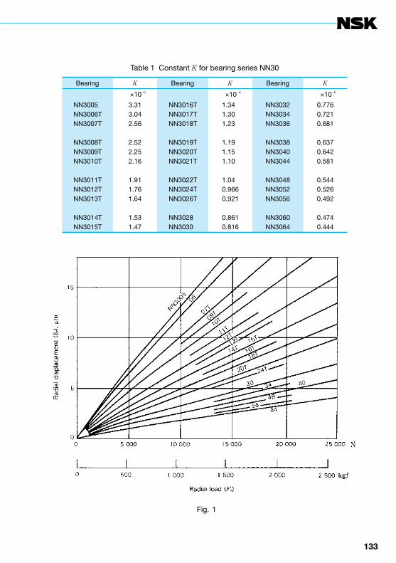
132 133

Table 1 Constant K for bearing series NN30

Bearing K Bearing K Bearing K

───×10−6 ───×10−6 ───×10−6

NN3005NN3006TNN3007T



NN3014TNN3015T

3.313.042.56

2.522.252.16

1.911.761.64

1.531.47




NN3028NN3030

1.341.301.23

1.191.151.10

1.040.9660.921

0.8610.816

NN3032NN3034NN3036

NN3038NN3040NN3044

NN3048NN3052NN3056

NN3060NN3064

0.7760.7210.681

0.6370.6420.581

0.5440.5260.492

0.4740.444

Fig. 1

134


5.8 Misalignment, maximum rolling-element load and moment for deep groove ball bearings

5.8.1 Misalignment angle of rings and　　 maximum rolling-element load

There are occasions when the inner and outer rings of deep groove bearings are forced to rotate out of parallel, whether from shaft deflection or mounting error. The allowable misalignment can be determined from the relation between the inner or outer ring deflection angle q and maximum rolling-element load Qmax.

For standard groove radii, the relation between q and Qmax (see Fig. 1) is given by Equation (1).

Qmax=K Dw2 q 2+cos2a0–1

3/2

(N), {kgf} ............................... (1)

where, K: Constant determined by bearing material and design

Approximately for deep groove ball bearing

K=717 (N-unit) K=72.7 {kgf-unit} Qmax: Maximum rolling element load (N),

{kgf} Dw: Ball diameter (mm) Ri: Distance between bearing center

and inner ring raceway curvature center (mm)

m0: m0=ri+re–Dw

ri and re are inner and outer ring groove radii, respectively

q: Inner and outer ring misalignment angle (rad)

a0: Initial contact angle (° )

cos a0=1–

Dr: Radial clearance (mm)

Fig. 2 shows the relationship between q and Qmax for a 6208 ball bearing with various radial clearances Dr.

When a radial load Fr equivalent to the basic static load rating C0r=17 800 N {1 820 kgf} or basic dynamic load rating Cr=29 100 N {2 970 kgf} is applied on a bearing, Qmax becomes as follows by Equation 8 in Section 5.1.

Fr=C0r Qmax=9 915 N {1 011 kgf}Fr=Cr Qmax=16 167 N {1 650 kgf}

Since the allowable misalignment q during operation will vary depending on the load, it is impossible to make an unqualified statement, but if we reasonably assume Qmax=2 000 N {204 kgf}, 20% of Qmax when Fr=C0r, we can determine from Fig. 2 that q will be:

Dr=0 q=18’Dr=0.050 mm q=24.5’

Ri

2m0( )

Dr

2m0

Fig. 1

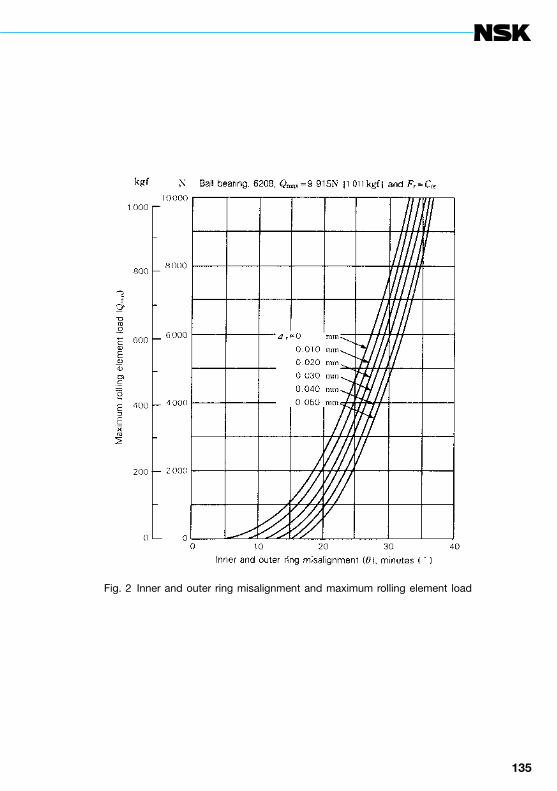
134 135

Fig. 2　Inner and outer ring misalignment and maximum rolling element load

136


5.8.2 Misalignment of inner and outer rings　　 and moment

To determine the angle y (Fig. 3) between the positions of the ball and ball under maximum rolling-element load, for standard race way radii, Equation (2) for rolling-element load Q (y) can be used like Equation (1) (Page 134).

Q (y)=K Dw2 q

2cos2y+cos2a0–1

3/2

(N), {kgf} ............................... (2)

The moment M (y) caused by the relative inner and outer ring misalignment from this Q (y) is given by,

M (y)= cos y Q (y) sina (y)

where, Dpw: Ball pitch diameter (mm) a (y), as used here, represents the local rolling element contact angle at the y position. It is given by,

q cos ysina (y)= q

2 cos2y+cos2a0

It is better to consider that the moment M originating from bearing can be replaced with the total moment originating from individual rolling element loads. The relation between the inner and outer ring misalignment angle q and moment M is as shown by Equation (3):

M= S cos yQ (y) sina (y)

=

(mN ·m), {kgf ·mm} ................ (3)

where, K: Constant determined by bearing material and design

Figs. 4 shows the calculated results for a 6208 deep groove ball bearing with various internal clearances. The allowable moment for a 6208 bearing with a maximum rolling element load Qmax of 2 000 N {204 kgf}, can be estimated using Fig. 2 (Page 135):

Radial clearance Dr=0, q=18’M=60 N ·m {6.2 kgf ·mm}

Radial clearance Dr=0.050 mm q=24.5’M=70 N ·m {7.1 kgf ·mm}

Ri

m0( )

Dpw

2

Ri

m0( )

Ri

m0( )

Dpw

2

2p

y=0

q 2cos2y+cos2a0–1

3/2

q cos2y S

q 2 cos2y+cos2a0

Ri

m0( ) Ri

m0( )

Ri

m0( )

KDpwDw2

2

Fig. 3

136 137

Fig. 4　Inner and outer ring misalignment and moment

138


5.9 Load distribution of single-direction thrust bearing due to eccentric load

When a pure axial load Fa is applied on a single-direction thrust bearing with a contact angle of a=90°, each rolling element is subjected to a uniform load Q:

Q=

where, Z: Number of rolling elementsFig. 1 shows the distribution with any

eccentric load Fa applied on a single-direction thrust bearing with a contact angle a=90°.

Based on Fig. 1, the following equations can be derived to determine the total elastic deformation dmax of the rolling element under the maximum load and the elastic deformation of any other rolling element d (y).

dmax=dT+ .............................................. (1)

d (y)=dT+ cosy .................................. (2)

From Equation (1) and (2) we obtain,

d (y)=dmax 1– (1– cosy) ...................... (3)

where,

ε = 1+ ....................................... (4)

The load Q (y) on any rolling element is proportional to the elastic deformation d (y) of the contact surface to the t power. Thus when y=0, with Qmax representing the maximum rolling element load and dmax the elastic deformation, we obtain.

= t

.......................................... (5)

t=1.5 (point contact), t=1.1 (line contact)

From Equations (3) and (5), we obtain,

=1– (1–cosy) t

......................... (6)

Since the eccentric load Fa acting on a bearing must be the sum of the individual rolling element loads, we obtain (Z is the number of the rolling elements),

Fa= S Q (y)

= S Qmax= 1– (1– cosy) t

=Qmax Z JA ................................................... (7)

Based on Fig. 1, the moment M acting on the shaft with y=90° as the axis is,

M= S Q (y) cosy

= S Qmax 1– (1–cosy) t

cosy

=Qmax Z JR ........................................... (8)

Values for ε and the corresponding JA and JR values for point contact and line contact from Equations (7) and (8) are listed in Table 1.

Sample CalculationFind the maximum rolling element load for a 51130X single-direction thrust ball bearing (f150×f190×31 mm) that sustains an axial load of 10 000 N {1 020 kgf} at a position 80 mm out from the bearing center.

e=80, Dpw≒ (150+190)=170

= =0.941

Z=32

Fa

Z

qDpw

2

1

2ε

1

22dT

qDpw( )

Q (y) Qmax

d (y)dmax

1

2ε

2p

y=0

2p

y=0

1

2ε

Dpw

2

2p

y=0

2p

y=0

1

2ε

1

2

2e

Dpw

2×80

170

qDpw

2

Dpw

2

Dpw

2

Q (y) Qmax

138 139

Using Table 1, the value for JA corresponding to 2e/Dpw=0.941 is 0.157. Substituting these values into Equation (7), we obtain,

Qmax= = =1 990 (N)

= =203 {kgf}

Fa

Z JA

10 00032×0.157

1 02032×0.157

Fig. 1

e: Distance between bearing center and loading pointDpw: Rolling-element pitch diameter

Table 1 JR and JA values for single-direction thrust bearings

εPoint contact Line contact

2e/Dpw

2M/Dpw Fa

JR JA2e/Dpw

2M/Dpw Fa

JR JA

00.10.2

0.30.40.5

0.60.70.8

0.91.01.25

1.672.55.0∞

1.00000.96630.9318

0.89640.86010.8225

0.78350.74270.6995

0.65290.60000.4338

0.30880.18500.08310

1/Z0.11560.1590

0.18920.21170.2288

0.24160.25050.2559

0.25760.25460.2289

0.18710.13390.07110

1/Z0.11960.1707

0.21100.24620.2782

0.30840.33740.3658

0.39450.42440.5044

0.60600.72400.85581.0000

1.00000.96130.9215

0.88050.83800.7939

0.74800.69990.6486

0.59200.52380.3598

0.23400.13720.06110

1/Z0.12680.1737

0.20550.22860.2453

0.25680.26360.2658

0.26280.25230.2078

0.15890.10750.05440

1/Z0.13190.1885

0.23340.27280.3090

0.34330.37660.4098

0.44390.48170.5775

0.67900.78370.89091.0000

140

6. Preload and axial displacement

6.1 Position preload and constant-pressure preload

Bearings for machine-tool head spindles, hypoid-gear pinion shafts, and other similar applications are often preloaded to increase bearing rigidity and, thereby, reduce as far as possible undesirable bearing displacement due to applied loads.

Generally, a preload is applied as shown in Fig. 1, using a spacer, shim, etc. to set the displacement dimensionally (position preload), or, as shown in Fig. 2, using a spring (constant pressure preload).

The effect of a position preload on rigidity is apparent in preload graphs such as Fig. 3. This graph is similar to data generally found in bearing makers’ catalogs. That is, Fig. 3 shows that the relation between the axial displacement da and external load Fa (axial load) under the preload of Fa0. This graph of position preload is derived from the displacement curves for the two side-by-side bearings, A and B.

By substituting a spring displacement curve (a straight line) for the bearing B displacement curve and plotting it together with the displacement curve for bearing A, a graph for a constant-pressure preload is formed.

Fig. 4 is a preload graph for a constant-pressure preload. Because spring rigidity is, as a rule, small compared with bearing rigidity, the displacement curve for the spring is a straight line that is nearly parallel to the horizontal axis of the graph. It also follows that an increase in rigidity under a constant-pressure preload will be nearly the same as an increase in rigidity for a single bearing subjected to an Fa0 preload.

Fig. 5 compares the rigidity provided by various preload methods on a 7212A angular contact ball bearing.

Fig. 1　Position preload

Fig. 2　Constant-pressure preload

Fig. 3　Preload graph for position preload

140 141

Fig. 4　Preload graph for constant-pressure preload

Fig. 5　Comparison of rigidity among different preload methods

142

Preload and axial displacement

6.2 Load and displacement of position-preloaded bearings

Two (or more) ball or tapered roller bearings mounted side by side as a set are termed duplex (or multiple) bearing sets. The bearings most often used in multiple arrangements are single-row angular contact ball bearings for machine tool spindles, since there is a requirement to reduce the bearing displacement under load as much as possible.

There are various ways of assembling sets depending on the effect desired. Duplex angular contact bearings fall into three types of arrangements, Back-to-Back, with lines of force convergent on the bearing back faces, Face-to-Face, with lines of force convergent on the bearing front faces, and Tandem, with lines of force being parallel. The symbols for these are DB, DF, and DT arrangements respectively (Fig. 1).

DB and DF arrangement sets can take axial loads in either direction. Since the distance of the load centers of DB bearing set is longer than that of DF bearing set, they are widely used in applications where there is a moment. DT type sets can only take axial loads in one direction. However, because the two bearings share some load equally between them, a set can be used where the load in one direction is large.

By selecting the DB or DF bearing sets with the proper preloads which have already been adjusted to an appropriate range by the bearing manufacturer, the radial and axial displacements of the bearing inner and outer ring can be reduced as much as allowed by certain limits. However, the DT bearing set cannot be preloaded.

The amount of preload can be adjusted by changing clearance between bearings, da0, as shown in Figs. 3 to 5. Preloads are divided into four graduated classification — Extra light (EL), Light (L), Medium (M), and Heavy (H). Therefore, DB and DF bearing sets are often used for applications where shaft misalignments and displacements due to loads must be minimized.

Triplex sets are also available in three types (symbols: DBD, DFD, and DTD) of arrangements as shown in Fig. 2. Sets of four or five bearings can also be used depending on the application requirements.

Duplex bearings are often used with a preload applied. Since the preload affects the rise in bearing temperature during operation, torque, bearing noise, and especially bearing life, it is extremely important to avoid applying an excessive preload.

Generally, the axial displacement da under an axial load Fa for single-row angular contact ball bearings is calculated as follows,

da=c Fa2/3 ..................................................... (1)

where, c: Constant depending on the bearing type and dimensions.

Fig. 3 shows the preload curves of duplex DB arrangement, and Figs. 4 and 5 show those for triplex DBD arrangement.

If the inner rings of the duplex bearing set in Fig. 3 are pressed axially, A-side and B-side bearings are deformed da0A and da0B respectively and the clearance (between the inner rings), da0, becomes zero. This condition means that the preload Fa0 is applied on the bearing set. If an external axial load Fa is applied on the preloaded bearing set from the A-side, then the A-side bearing will be deformed da1 additionally and the displacement of B-side bearing will be reduced to the same amount as the A-side bearing displacement da1. Therefore, the displacements of A- and B-side bearings are daA=da0A+da1 and daB=da0B+da1 respectively. That is, the load on A-side bearing including the preload is (Fa0+Fa–Fa’) and the B-side bearing is (Fa0–Fa’).

142 143

Fig. 1　Duplex bearing arrangements　　　

Fig. 2　Triplex bearing arrangements

Fig. 3　Preload graph of DB arrangement duplex bearings

144


If the bearing set has an applied preload, the A-side bearing should have a sufficient life and load capacity for an axial load (Fa0+Fa–Fa’) under the speed condition. The axial clearance da0 is shown in Tables 3 to 7 of Section 6.3 (Pages 151 to 155).

In Fig. 4, with an external axial load Fa applied on the AA-side bearings, the axial loads and displacements of AA- and B-side bearings are summarized in Table 1.

In Fig. 5, with an external axial load Fa applied on the A-side bearing, the axial loads and displacements of A- and BB-side bearings are summarized in Table 2.

The examples, Figs. 6 to 11, show the relation of the axial loads and axial displacements using duplex DB and triplex DBD arrangements of 7018C and 7018A bearings under several preload ranges.

Fig. 4　Preload graph of triplex DBD bearing set (Axial load is applied from AA-side)

Table 1

Direction Displacement Axial load

AA-side da0A＋da1 Fa0＋Fa−Fa′B-side da0B−da1 Fa0−Fa′

Table 2

Direction Displacement Axial load

A-side da0A＋da1 Fa0＋Fa−Fa′BB-side da0B−da1 Fa0−Fa′

144 145

Fig. 5　Preload graph of triplex DBD bearing set (Axial load is applied from A-side)

146


Fig. 6

Fig. 7

146 147

Fig. 8

Remarks A (◯) mark on the axial load or displacement curve indicates the point where the preload is zero. Therefore, if the axial load is larger than this, the opposed bearing does not impose a load.

148


Fig. 10

Fig. 9

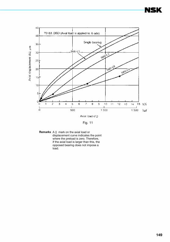
148 149

Fig. 11

Remarks A (◯) mark on the axial load or displacement curve indicates the point where the preload is zero. Therefore, if the axial load is larger than this, the opposed bearing does not impose a load.

150


6.3 Average preload for duplex angular contact ball bearings

Angular contact ball bearings are widely used in spindles for grinding, milling, high-speed turning, etc. At NSK, preloads are divided into four graduated classifications — Extra light (EL), Light (L), Medium (M), and Heavy (H) — to allow the customer to freely choose the appropriate preload for the specific application. These four preload classes are expressed in symbols, EL, L, M, and H, respectively, when applied to DB and DF bearing sets.

The average preload and axial clearance (measured) for duplex angular contact ball bearing sets with contact angles 15° and 30° (widely used on machine tool spindles) are given in Tables 3 to 7.

The measuring load when measuring axial clearance is shown in Table 1.

The recommended axial clearance to achieve the proper preload was determined for machine-tool spindles and other applications requiring ISO Class 5 and above high-precision bearing sets. The standard values given in Table 2 are used for the shaft — inner ring and housing — outer ring fits. The housing fits shouldbe selected in the lower part of the standard clearance for bearings in fixed-end applications and the higher part of the standard clearance for bearings in free-end applications.

As general rules when selecting preloads, grinding machine spindles or machining center spindles require extra light to light preloads, whereas lathe spindles, which need rigidity, require medium preloads.

The bearing preloads, if the bearing set is mounted with tight fit, are larger than those shown in Tables 3 to 7. Since excessive preloads cause bearing temperature rise and seizure, etc., it is necessary to pay attention to fitting.

*10 mm is included in this range.

Table 1 Measuring load of axial clearance

◯◯Nominal bearingoutside diameter D (mm) Measuring load

over incl (N)

10* 50120200

50120200

◯

24.54998

196

Table 2 Target of fittingUnits: μm

Bore or outside diameterd or D (mm)

Shaft andinner ring

Housing andouter ring

over incl Target interference Target clearance

◯

18

30

50

80

120

150

180

18

30

50

80

120

150

180

250

0 to 2

0 to 2.5

0 to 2.5

0 to 3

0 to 4

◯

◯

◯

◯

2 to 6

2 to 6

3 to 8

3 to 9

4 to 12

4 to 12

5 to 15

150 151

Remarks　In the axial clearance column, the measured value is given.

Table 3 Average preloads and axial clearance for bearing series 79C

Bearing

No.

Extra light EL Light L Medium M Heavy H

PreloadAxial

clearancePreload

Axialclearance

PreloadAxial

clearancePreload

Axialclearance

(N) (μm) (N) (μm) (N) (μm) (N) (μm)

7900C

7901C

7902C

7903C

7904C

7905C

7906C

7907C

7908C

7909C

7910C

7911C

7912C

7913C

7914C

7915C

7916C

7917C

7918C

7919C

7920C

7

8.6

12

12

19

19

24

34

39

50

50

60

60

75

100

100

100

145

145

145

195

◯5

◯4

◯3

◯3

◯1

◯1

◯0

◯2

◯1

◯0

◯0

−1

−1

−2

−4

−4

−4

−6

−3

−3

−5

15

15

25

25

39

39

49

69

78

100

100

120

120

150

200

200

200

290

290

290

390

◯ 2

◯ 2

◯ 0

◯0

−3

−2

−3

−2

−3

−5

−4

−5

−5

−7

−10

−9

−9

−14

−9

−9

−13

29

39

49

59

78

100

100

150

200

200

250

290

290

340

490

490

490

640

740

780

880

−1

−3

−4

−5

−8

−9

−8

−9

−12

−11

−13

−15

−15

−16

−22

−21

−21

−25

−23

−24

−28

59

78

100

120

150

200

200

290

390

390

490

590

590

690

980

980

980

1 270

1 470

1 570

1 770

−6

−8

−11

−12

−15

−17

−16

−18

−22

−21

−24

−26

−25

−27

−36

−35

−34

−41

−39

−40

−46

152




Bearing

No.


PreloadAxial

clearancePreload

Axialclearance

PreloadAxial

clearancePreload

Axialclearance

(N) (μm) (N) (μm) (N) (μm) (N) (μm)

7000C

7001C

7002C

7003C

7004C

7005C

7006C

7007C

7008C

7009C

7010C

7011C

7012C

7013C

7014C

7015C

7016C

7017C

7018C

7019C

7020C

12

12

14

14

24

29

39

60

60

75

75

100

100

125

145

145

195

195

245

270

270

◯3

◯3

◯3

◯2

◯0

−1

◯1

−1

−1

−3

−2

−4

−4

−6

−7

−7

−6

−6

−8

−9

−9

25

25

29

29

49

59

78

120

120

150

150

200

200

250

290

290

390

390

490

540

540

◯ 0

◯ 0

−1

−1

−4

−5

−3

−7

−6

−8

−8

−11

−10

−13

−14

−14

−14

−14

−18

−19

−18

49

59

69

69

120

150

200

250

290

340

390

490

540

540

740

780

930

980

1 180

1 180

1 270

−5

−6

−7

−7

−12

−14

−13

−16

−17

−19

−20

−24

−25

−24

−30

−31

−31

−32

−37

−36

−37

100

120

150

150

250

290

390

490

590

690

780

980

1 080

1 080

1 470

1 570

1 860

1 960

2 350

2 350

2 550

−12

−14

−16

−16

−22

−24

−24

−28

−30

−33

−34

−40

−42

−39

−48

−49

−52

−52

−60

−58

−60

152 153



Bearing

No.


PreloadAxial

clearancePreload

Axialclearance

PreloadAxial

clearancePreload

Axialclearance

(N) (μm) (N) (μm) (N) (μm) (N) (μm)

7200C

7201C

7202C

7203C

7204C

7205C

7206C

7207C

7208C

7209C

7210C

7211C

7212C

7213C

7214C

7215C

7216C

7217C

7218C

7219C

7220C

14

19

19

24

34

39

60

75

100

125

125

145

195

220

245

270

295

345

390

440

490

◯ 3

◯ 1

◯ 1

◯ 0

−2

◯ 1

−1

−3

−5

−7

−7

−8

−11

−12

−9

−10

−12

−14

−15

−18

−20

29

39

39

49

69

78

120

150

200

250

250

290

390

440

490

540

590

690

780

880

980

−1

−3

−3

−4

−7

−4

−7

−10

−13

−16

−15

−17

−22

−23

−20

−21

−24

−27

−29

−33

−36

69

100

100

150

200

200

290

390

490

540

590

780

930

1 080

1 180

1 230

1 370

1 670

1 860

2 060

2 350

−8

−12

−11

−16

−20

−14

−20

−25

−29

−30

−31

−38

−42

−44

−42

−42

−47

−53

−57

−63

−68

150

200

200

290

390

390

590

780

980

1 080

1 180

1 570

1 860

2 160

2 350

2 450

2 750

3 330

3 730

4 120

4 710

−18

−22

−21

−28

−33

−27

−35

−43

−47

−49

−50

−60

−67

−70

−69

−68

−76

−85

−90

−99

−107

154



Table 6 Average preloads and axial clearance for bearing series 70A

Bearing

No.


PreloadAxial

clearancePreload

Axialclearance

PreloadAxial

clearancePreload

Axialclearance

(N) (μm) (N) (μm) (N) (μm) (N) (μm)

7000A

7001A

7002A

7003A

7004A

7005A

7006A

7007A

7008A

7009A

7010A

7011A

7012A

7013A

7014A

7015A

7016A

7017A

7018A

7019A

7020A

25

25

25

25

25

25

50

50

50

50

50

50

50

50

50

50

100

100

100

100

100

0

0

0

0

0

0

0

0

0

0

0

0

0

0

0

0

0

0

0

0

0

100

110

110

120

130

140

190

210

220

230

250

250

250

270

270

280

760

780

780

810

840

−5

−5

−5

−5

−5

−5

−5

−5

−5

−5

−5

−5

−5

−5

−5

−5

−10

−10

−10

−10

−10

210

220

240

250

280

290

390

420

460

480

530

880

930

980

1 080

1 080

1 770

1 860

2 450

2 550

2 750

−10

−10

−10

−10

−10

−10

−10

−10

−10

−10

−10

−15

−15

−15

−15

−15

−20

−20

−25

−25

−25

330

360

390

420

470

510

640

700

760

1 180

1 270

1 270

1 370

1 470

2 060

2 160

3 040

3 240

3 920

4 120

4 310

−15

−15

−15

−15

−15

−15

−15

−15

−15

−20

−20

−20

−20

−20

−25

−25

−30

−30

−35

−35

−35

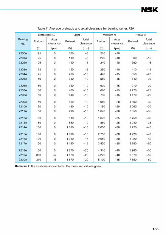
154 155


Table 7 Average preloads and axial clearance for bearing series 72A

Bearing

No.


PreloadAxial

clearancePreload

Axialclearance

PreloadAxial

clearancePreload

Axialclearance

(N) (μm) (N) (μm) (N) (μm) (N) (μm)

7200A

7201A

7202A

7203A

7204A

7205A

7206A

7207A

7208A

7209A

7210A

7211A

7212A

7213A

7214A

7215A

7216A

7217A

7218A

7219A

7220A

25

25

25

25

25

50

50

50

50

50

50

50

50

50

100

100

100

100

100

360

370

◯0

◯0

◯0

◯0

◯0

◯0

◯0

◯0

◯0

◯0

◯0

◯0

◯0

◯0

◯0

◯0

◯0

◯0

◯0

−5

−5

100

110

110

120

260

350

380

400

440

450

480

490

510

550

1 080

1 080

1 080

1 180

1 670

1 670

1 670

−5

−5

−5

−5

−10

−10

−10

−10

−10

−10

−10

−10

−10

−10

−15

−15

−15

−15

−20

−20

−20

210

220

240

250

440

580

630

660

730

1 080

1 180

1 670

1 670

1 860

2 650

2 750

2 650

3 430

4 310

4 220

5 100

−10

−10

−10

−10

−15

−15

−15

−15

−15

−20

−20

−26

−25

−25

−30

−30

−30

−35

−40

−40

−45

◯

360

390

410

650

840

910

1 270

1 470

1 860

2 060

2 650

2 750

3 040

3 920

4 220

4 020

5 790

5 980

6 670

7 650

◯

−15

−15

−15

−20

−20

−20

−25

−25

−30

−30

−35

−35

−35

−40

−40

−40

−50

−50

−55

−60

156


6.4 Axial displacement of deep groove ball bearings

When an axial load Fa is applied to a radial bearing with a contact angle a0 and the inner ring is displaced da, the center Oi of the inner ring raceway radius is also moved to Oi’ resulting in the contact angle a as shown in Fig. 1. If dN represents the elastic deformation of the raceway and ball in the direction of the rolling element load Q, Equation (1) is derived from Fig. 1.

(m0+dN)2=(m0·sina0+da)2+(m0·cosa0)2

\ dN=m0 sina0+ 2

+cos2a0– 1 ............. (1)

Also there is the following relationship between the rolling element load Q and elastic deformation dN.

Q=KN·dN3/2 ................................................... (2)

where, KN: Constant depending on bearing material, type, and dimension

\ If we introduce the relation of

m0= + – 1 Dw=B ·Dw

Equations (1) and (2) are,

Q=KN (B ·Dw)3/2 (sina0+h)2+cos2a0–1 3/2

where, h= =

If we introduce the relation of KN=K ·

Q=K ·Dw2 　 (sina0+h)2+cos2a0–1

3/2 ................... (3)

On the other hand, the relation between the bearing axial load and rolling element load is shown in Equation (4) using Fig. 2:

Fa=Z ·Q ·sina .............................................. (4)

Based on Fig. 1, we obtain,

(m0+dN) sina=m0·sina0+da

\ sina= =

If we substitute Equation (1),

sina= ............................. (5)

That is, the relation between the bearing axial load Fa and axial displacement da can be obtained by substituting Equations (3) and (5) for Equation (4).

Fa=K ·Z ·Dw2 ·

........................................ (6)

where, K: Constant depending on the bearing material and design

Dw: Ball diameter Z: Number of balls a0: Initial contact angle In case of single-row deep groove

ball bearings, the initial contact angle can be obtained using Equation (5) of Section 4.6 (Page 96)

Actual axial deformation varies depending on the bearing mounting conditions, such as the material and thickness of the shaft and housing, and bearing fitting. For details, consult with NSK regarding the axial deformation after mounting.

( )da

m0

re

Dw

ri

Dw( )

√—————————

da

m0

da

B ·Dw

Dw

B3/2

√—

√—————————

m0·sina0+da

m0+dN

sina0+h

1+ dN

m0

sina0+h(sina0+h)2+cos2a0√—————————

(sina0+h)2+cos2a0–1 3/2

´(sina0+h)(sina0+h)2+cos2a0√—————————

√—————————

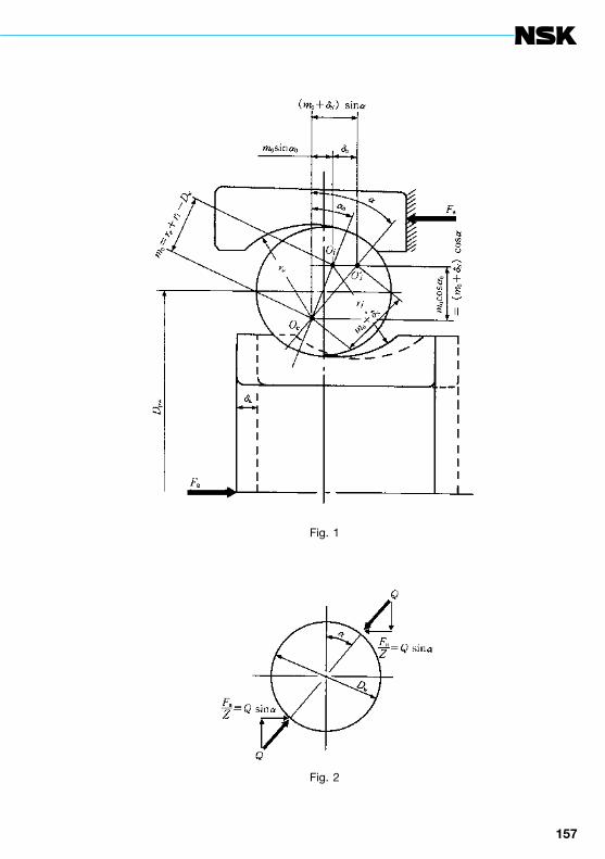
156 157

Fig. 1

Fig. 2

158


Fig. 3 gives the relation between axial load and axial displacement for 6210 and 6310 single-row deep groove ball bearings with initial contact angles of a0=0°, 10°, 15°. The larger the initial contact angle a0, the more rigid the bearing will be in the axial direction and also the smaller the difference between the axial displacements of 6210 and 6310 under the same axial load. The angle a0 depends upon the groove radius and the radial clearance.

Fig. 4 gives the relation between axial load and axial displacement for 72 series angular contact ball bearings with initial contact angles of 15° (C), 30° (A), and 40° (B). Because 70 and 73 series bearings with identical contact angles and bore diameters can be considered to have almost the same values as 72 series bearings.

Angular contact ball bearings that sustain loads in the axial direction must maintain their running accuracy and reduce the bearing elastic deformation from applied loads when used as multiple bearing sets with a preload applied.

To determine the preload to keep the elastic deformation caused by applied loads within the required limits, it is important to know the characteristics of load vs. deformation. The relationship between load and displacement can be expressed by Equation (6) as Fa∝da

3/2 or da∝Fa

3/2. That is, the axial displacement da is proportional to the axial load Fa to the 2/3 power. When this axial load index is less than one, it indicates the relative axial displacement will be small with only a small increase in the axial load. (Fig. 4) The underlying reason for applying a preload is to reduce the amount of displacement.

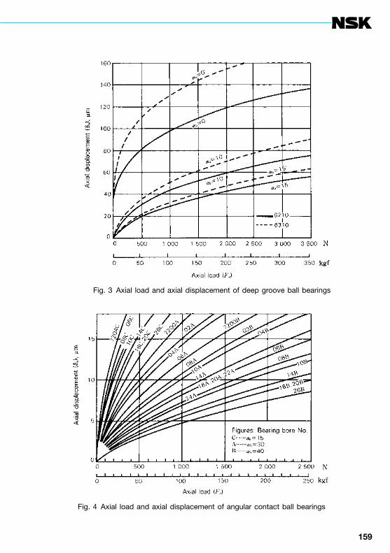
158 159

Fig. 3　Axial load and axial displacement of deep groove ball bearings

Fig. 4　Axial load and axial displacement of angular contact ball bearings

160


6.5 Axial displacement of tapered roller bearings

Tapered roller bearings are widely used in pairs like angular contact ball bearings. Care should be taken to select appropriate tapered roller bearings.

For example, the bearings of machine tool head spindles and automobile differential pinions are preloaded to increase shaft rigidity.

When a bearing with an applied preload is to be used in an application, it is essential to have some knowledge of the relationship between axial load and axial displacement. For tapered roller bearings, the axial displacement calculated using Palmgren’s method, Equation (1) generally agrees well with actual measured values.

Actual axial deformation varies depending on the bearing mounting conditions, such as the material and thickness of the shaft and housing, and bearing fitting. For details, consult with NSK regarding the axial deformation after mounting.

da= · (N) ......... (1)

= · {kgf}

where, da: Axial displacement of inner, outer ring (mm)

a: Contact angle...1/2 the cup angle (°) Q: Load on rolling elements (N), {kgf}

Q=

Lwe: Length of effective contact on roller (mm)

Fa: Axial load (N), {kgf} Z: Number of rollers

Equation (1) can also be expressed as Equation (2).

da=Ka·Fa0.9 ................................................... (2)

where,Ka= ................................ (N)

= ............................. {kgf}

Here, Ka: Coefficient determined by the bearing internal design.

Axial loads and axial displacement for tapered roller bearings are plotted in Fig. 1.

The amount of axial displacement of tapered roller bearings is proportional to the axial load raised to the 0.9 power. The displacement of ball bearings is proportional to the axial load raised to the 0.67 power, thus the preload required to control displacement is much greater for ball bearings than for tapered roller bearings.

Caution should be taken not to make the preload indiscriminately large on tapered roller bearings, since too large of a preload can cause excessive heat, seizure, and reduced bearing life.0.000077

sinaQ0.9

Lwe0.8

0.0006sina

Q0.9

Lwe0.8

Fa

Zsina

0.00007(sina)1.9 Z 0.9 Lwe

0.8

0.0006(sina)1.9 Z 0.9 Lwe

0.8

160 161

Fig. 1　Axial load and axial displacement for tapered roller bearings

162

7. Starting and running torques

7.1 Preload and starting torque for angular contact ball bearings

Angular contact ball bearings, like tapered roller bearings, are most often used in pairs rather than alone or in other multiple bearing sets. Back-to-back and face-to-face bearing sets can be preloaded to adjust bearing rigidity. Extra light (EL), Light (L), Medium (M), and Heavy (H) are standard preloads. Friction torque for the bearing will increase in direct proportion to the preload.

The starting torque of angular contact ball bearings is mainly the torque caused by angular slippage between the balls and contact surfaces on the inner and outer rings. Starting torque for the bearing M due to such spin is given by,

M=Ms·Zsina (mN ·m), {kgf ·mm} ................. (1)

where, Ms: Spin friction for contact angle a centered on the shaft,

Ms= ms·Q ·a E (k)

(mN ·m), {kgf ·mm} ms: Contact-surface slip friction

coefficient Q: Load on rolling elements (N), {kgf} a: (1/2) of contact-ellipse major axis

(mm)

E (k): With k= 1– 2

as the population parameter, second class complete ellipsoidal integration

b: (1/2) of contact-ellipse minor axis (mm)

Z: Number of balls a: Contact angle (° )

Actual measurements with 15° angular contact ball bearings correlate well with calculated results using ms=0.15 in Equation (1). Fig. 1 shows the calculated friction torque for 70C and 72C series bearings.

ba( )

38

162 163

Fig. 1　Preload and starting torque for angular contact ball bearings (a=15°) of DF and DB duplex sets

164

Starting and running torques

7.2 Preload and starting torque for tapered roller bearings

The balance of loads on the bearing rollers when a tapered roller bearing is subjected to axial load Fa is expressed by the following three Equations (1), (2), and (3):

Qe= ............................................... (1)

Qi=Qecos2b= Fa ........................... (2)

Qf=Qesin2b= Fa ............................ (3)

where, Qe: Rolling element load on outer ring (N), {kgf}

Qi: Rolling element load on inner ring (N), {kgf}

Qf: Rolling element load on inner-ring large end rib, (N), {kgf} (assume Qf ^ Qi)

Z: Number of rollers a: Contact angle...(1/2) of the cup

angle (° ) b: (1/2) of tapered roller angle (° ) Dw1: Roller large-end diameter (mm)

(Fig. 1) e: Contact point between roller end

and rib (Fig. 1)

As represented in Fig. 1, when circumferential load F is applied to the bearing outer ring and the roller turns in the direction of the applied load, the starting torque for contact point C relative to instantaneous center A becomes e meQf.

Therefore, the balance of frictional torque is,

Dw1F=e meQf (mN ·m), {kgf ·mm} ................. (4)

where, me: Friction coefficient between inner ring large rib and roller endface

The starting torque M for one bearing is given by,

M=F Z l

= Fa

(mN ·m), {kgf ·mm} ................ (5)

because, Dw1=2 OB sin b, and l=OB sin a.If we substitute these into Equation (5) we obtain,

M=e me cosb Fa (mN ·m), {kgf ·mm} .......................................... (6)

The starting torque M is sought considering only the slip friction between the roller end and the inner-ring large-end rib. However, when the load on a tapered roller bearing reaches or exceeds a certain level (around the preload) the slip friction in the space between the roller end and inner-ring large end rib becomes the decisive factor for bearing starting torque. The torque caused by other factors can be ignored. Values for e and b in Equation (5) are determined by the bearing design. Consequently, assuming a value for me, the starting torque can be calculated.

The values for me and for e have to be thought of as a dispersion, thus, even for bearings with the same number, the individual starting torques can be quite diverse. When using a value for e determined by the bearing design, the average value for the bearing starting torque can be estimated using me=0.20 which is the average value determined from various test results.

Fig. 2 shows the results of calculations for various tapered roller bearing series.

cos 2bZ sin a

sin 2bZ sin a

e me l sin 2bDw1 sin a

Fa

Z sin a

164 165

Fig. 1

Fig. 2　Axial load and starting torque for tapered roller bearings

166


7.3 Empirical equation of running torque of high-speed ball bearings

We present here empirical equations for the running torque of high speed ball bearings subject to axial loading and jet lubrication. These equations are based on the results of tests of angular contact ball bearings with bore diameters of 10 to 30 mm, but they can be extrapolated to bigger bearings.

The running torque M can be obtained as the sum of a load term Ml and speed term Mv as follows:

M=Ml+Mv (mN ·m), {kgf ·mm} ..................... (1)

The load term Ml is the term for friction, which has no relation with speed or fluid friction, and is expressed by Equation (2) which is based on experiments.

Ml=0.672´10–3Dpw0.7Fa

1.2 (mN ·m) .............. (2)=1.06´10–3Dpw

0.7Fa1.2 {kgf ·mm}

where, Dpw: Pitch diameter of rolling elements (mm)

Fa: Axial load (N), {kgf}

The speed term Mv is that for fluid friction, which depends on angular speed, and is expressed by Equation (3).

Mv=3.47´10–10Dpw3ni

1.4ZBaQb (mN ·m)

=3.54´10–11Dpw3ni

1.4ZBaQb {kgf ·mm}

......................................... (3)

where, ni: Inner ring speed (min–1) ZB: Absolute viscosity of oil at outer ring

temperature (mPa ·s), {cp} Q: Oil flow rate (kg/min)

The exponents a and b, that affect the oil viscosity and flow rate factors, depend only on the angular speed and are given by Equations (4) and (5) as follows:

a=24ni–0.37 ....................................................... (4)

b=4´10–9ni1.6+0.03 ......................................... (5)

An example of the estimation of the running torque of high speed ball bearings is shown in Fig. 1. A comparison of values calculated using these equations and actual measurements is shown in Fig. 2. When the contact angle exceeds 30°, the influence of spin friction becomes big, so the running torque given by the equations will be low.

Calculation ExampleObtain the running torque of high speed

angular contact ball bearing 20BNT02 (f20´f47´14) under the following conditions:

ni=70 000 min–1

Fa=590 N, {60 kgf}Lubrication: Jet, oil viscosity:

10 mPa ·s {10 cp}oil flow: 1.5 kg/min

From Equation (2),Ml=0.672´10–3Dpw

0.7Fa1.2

=0.672´10–3´33.50.7´5901.2

=16.6´10–3 (mN ·m)Ml=1.06´10–333.50.7´601.2=1.7

{kgf ·mm}

From Equations (4) and (5),a=24ni

–0.37

=24´70 000–0.37=0.39b=4´10–9ni

1.6+0.03=4´10–9´70 0001.6+0.03=0.26

From Equation (3),Mv=3.47´10–10Dpw

3ni1.4ZB

aQb

=3.47´10–10´33.53´70 0001.4´100.39´1.50.26

=216 (mN ·m)Mv=3.54´10–11´33.53´70 0001.4´100.39´1.50.26

=22.0 {kgf ·mm}M=Ml+Mv=16.6+216=232.6 (mN ·m)M=Ml+Mv=1.7+22=23.7 {kgf ·mm}

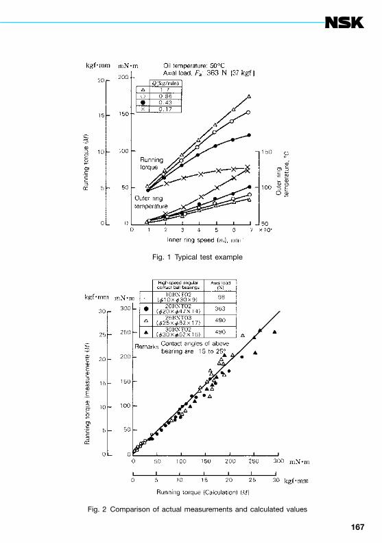
166 167

Fig. 1　Typical test example

Fig. 2　Comparison of actual measurements and calculated values

168


7.4 Empirical equations for running torque of tapered roller bearings

When tapered roller bearings operate under axial load, we reanalyzed the torque of tapered roller bearings based on the following two kinds of resistance, which are the major components of friction:(1) Rolling resistance (friction) of rollers with

outer or inner ring raceways — elastic hysteresis and viscous rolling resistance of EHL

(2) Sliding friction between inner ring ribs and roller ends

When an axial load Fa is applied on tapered roller bearings, the loads shown in Fig. 1 are applied on the rollers.

Qe≒Qi= .......................................... (1)

Qf= ............................................. (2)

where, Qe: Rolling element load on outer ring Qi: Rolling element load on inner ring Q f: Rolling element load on inner-ring

large end rib Z: Number of rollers a: Contact angle…(1/2) of the cup

angle b: (1/2) of tapered roller angle

For simplification, a model using the average diameter Dwe as shows in Fig. 2 can be used.

Where, Mi, Me: Rolling resistance (moment)

Fsi, Fse, Fsf: Sliding friction Ri, Re: Radii at center of inner

and outer ring raceways e: Contact height of roller

end face with rib

In Fig. 2, when the balance of sliding friction and moments on the rollers are considered, the following equations are obtained:

Fse–Fsi=Fsf ................................................... (3)

Mi+Me= Fse+ Fsi+ –e Fsf

............................................. (4)

When the running torque M applied on the outer (inner) ring is calculated using Equations (3) and (4) and multiplying by Z, which is the number of rollers:

M=Z (Re Fse–Me)

= (Re Mi+RiMe)+ Re e Fsf

=MR+MS

Therefore, the friction on the raceway surface MR and that on the ribs MS are separately obtained. Additionally, MR and MS are rolling friction and sliding friction respectively.

Fa

Z sina

Fa sin 2bZ sina

Dw

2 ( )Dw

2Dw

2

ZDw

ZDw

168 169

Fig. 1　Loads applied on roller

Fig. 2　Model of parts where friction is generated

170


The running torque M of a tapered roller bearing can be obtained from the rolling friction on the raceway MR and sliding friction on the ribs MS.

M=MR+MS= (Re Mi+Ri Me )

+ Re e Fsf ........................................... (5)

Sliding friction on rib MS

As a part of MS, Fsf is the tangential load caused by sliding, so we can write Fsf = mQf using the coefficient of dynamic friction m. Further, by substitution of the axial load Fa,the following equation is obtained:

MS = e m cosb Fa ........................................ (6)

This is the same as the equation for starting torque, but m is not constant and it decreases depending on the conditions or running in. For this reason, Equation (6) can be rewritten as follows:

MS=e m0 cosb Fa f ’ (L, t, s) ........................ (7)

Where m0 is approximately 0.2 and f ’ (L, t, s) is a function which decreases with running in and oil film formation, but it is set equal to one when starting.

Rolling friction on raceway surface MR

Most of the rolling friction on the raceway is viscous oil resistance (EHL rolling resistance). Mi and Me in Equation (5) correspond to it. A theoretical equation exists, but it should be corrected as a result of experiments. We obtained the following equation that includes corrective terms:

Mi, e= f (w)

(G ·U)0.658W 0.0126R2Lwe i, e

..................... (8)

f (w)= 0.3

............................. (9)

Therefore, MR can be obtained using Equations (8) and (9) together with the following equation:

MR= (Re Mi+Ri Me )

Running torque of bearings MFrom these, the running torque of tapered

roller bearings M is given by Equation (10)

M= (Re Mi+Ri Me )+e m0 cosb Fa f ’ (L, t, s)

....................................... (10)

As shown in Figs. 3 and 4, the values obtained using Equation (10) correlate rather well with actual measurements. Therefore, estimation of running torque with good accuracy is possible. When needed, please consult NSK.

[Explanation of Symbols]G, W, U: EHL dimensionless parametersL: Coefficient of thermal loada0: Pressure coefficient of lubricating oil

viscosityR: Equivalent radiusk: ConstantE’: Equivalent elastic modulusa: Contact angle (Half of cup angle)Ri , Re : Inner and outer ring raceway radii

(center)b: Half angle of rolleri, e: Indicate inner ring or outer ring

respectivelyLwe: Effective roller length

ZDw

ZDw

( 11+0.29L0.78

4.318a0

)[

]kFa

E’ DwLweZsina( )

ZDw

ZDw

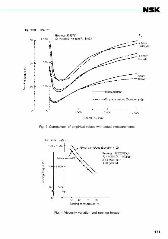
170 171

Fig. 3　Comparison of empirical values with actual measurements

Fig. 4　Viscosity variation and running torque

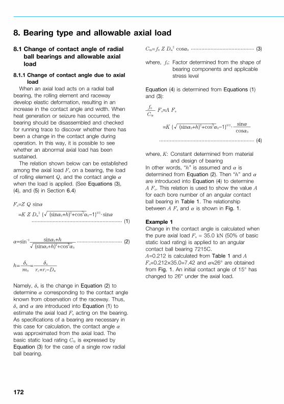
172

8. Bearing type and allowable axial load

8.1 Change of contact angle of radial ball bearings and allowable axial load

8.1.1 Change of contact angle due to axial 　　　load

When an axial load acts on a radial ball bearing, the rolling element and raceway develop elastic deformation, resulting in an increase in the contact angle and width. When heat generation or seizure has occurred, the bearing should be disassembled and checked for running trace to discover whether there has been a change in the contact angle during operation. In this way, it is possible to see whether an abnormal axial load has been sustained.

The relation shown below can be established among the axial load Fa on a bearing, the load of rolling element Q, and the contact angle a when the load is applied. (See Equations (3), (4), and (5) in Section 6.4)

Fa=Z Q sina

=K Z Dw2 { (sina0+h)2+cos2a0–1}3/2·sina

............................................................ (1)

a=sin–1 .............................. (2)

h= =

Namely, da is the change in Equation (2) to determine a corresponding to the contact angle known from observation of the raceway. Thus, da and a are introduced into Equation (1) to estimate the axial load Fa acting on the bearing. As specifications of a bearing are necessary in this case for calculation, the contact angle a was approximated from the axial load. The basic static load rating C0r is expressed by Equation (3) for the case of a single row radial ball bearing.

C0r= f0 Z Dw2 cosa0 .......................................... (3)

where, f0: Factor determined from the shape of bearing components and applicable stress level

Equation (4) is determined from Equations (1) and (3):

Fa=A Fa

=K { (sina0+h)2+cos2a0–1}3/2·

............................................................... (4)

where, K: Constant determined from material and design of bearing

In other words, “h” is assumed and a is determined from Equation (2). Then “h” and a are introduced into Equation (4) to determine A Fa. This relation is used to show the value A for each bore number of an angular contact ball bearing in Table 1. The relationship between A Fa and a is shown in Fig. 1.

Example 1Change in the contact angle is calculated when the pure axial load Fa = 35.0 kN (50% of basic static load rating) is applied to an angular contact ball bearing 7215C.A=0.212 is calculated from Table 1 and A Fa=0.212´35.0=7.42 and a≒26° are obtained from Fig. 1. An initial contact angle of 15° has changed to 26° under the axial load.

sina0+h(sina0+h)2+cos2a0

√—————————

√—————————

da

m0

da

re+ri–Dw

f0

C0r

√————————— sinacosa0

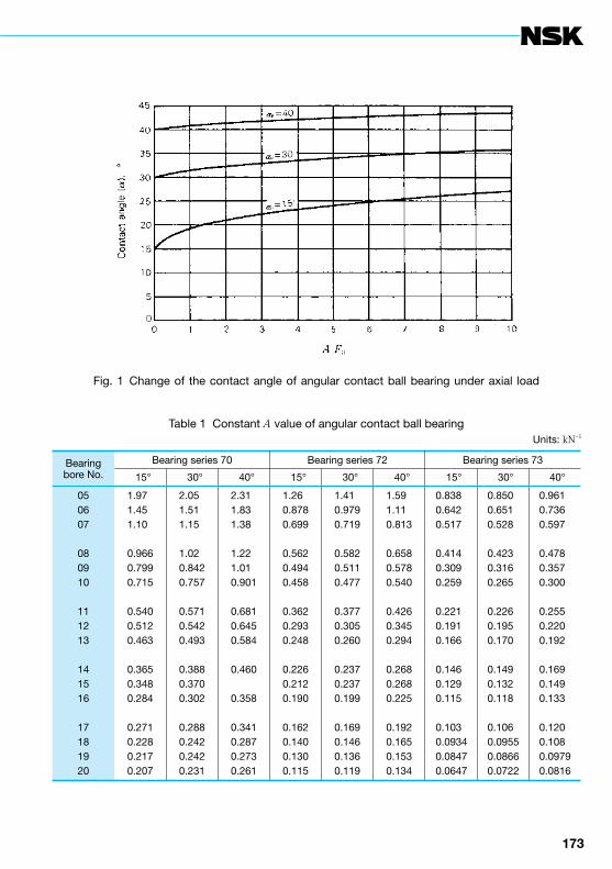
172 173

Fig. 1　Change of the contact angle of angular contact ball bearing under axial load

Table 1 Constant A value of angular contact ball bearingUnits: kN−1

Bearingbore No.

Bearing series 70 Bearing series 72 Bearing series 73

15° 30° 40° 15° 30° 40° 15° 30° 40°

050607

080910

111213

141516

17181920

1.971.451.10

0.9660.7990.715

0.5400.5120.463

0.3650.3480.284

0.2710.2280.2170.207

2.051.511.15

1.020.8420.757

0.5710.5420.493

0.3880.3700.302

0.2880.2420.2420.231

2.311.831.38

1.221.010.901

0.6810.6450.584

0.460―

0.358

0.3410.2870.2730.261

1.260.8780.699

0.5620.4940.458

0.3620.2930.248

0.2260.2120.190

0.1620.1400.1300.115

1.410.9790.719

0.5820.5110.477

0.3770.3050.260

0.2370.2370.199

0.1690.1460.1360.119

1.591.110.813

0.6580.5780.540

0.4260.3450.294

0.2680.2680.225

0.1920.1650.1530.134

0.8380.6420.517

0.4140.3090.259

0.2210.1910.166

0.1460.1290.115

0.1030.09340.08470.0647

0.8500.6510.528

0.4230.3160.265

0.2260.1950.170

0.1490.1320.118

0.1060.09550.08660.0722

0.9610.7360.597

0.4780.3570.300

0.2550.2200.192

0.1690.1490.133

0.1200.1080.09790.0816

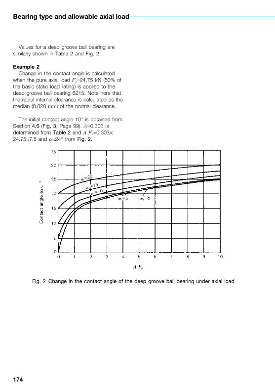
174

Bearing type and allowable axial load

Values for a deep groove ball bearing are similarly shown in Table 2 and Fig. 2.

Example 2Change in the contact angle is calculated

when the pure axial load Fa=24.75 kN (50% of the basic static load rating) is applied to the deep groove ball bearing 6215. Note here that the radial internal clearance is calculated as the median (0.020 mm) of the normal clearance.

The initial contact angle 10° is obtained from Section 4.6 (Fig. 3, Page 99). A=0.303 is determined from Table 2 and A Fa=0.303´ 24.75≒7.5 and a≒24° from Fig. 2.

Fig. 2　Change in the contact angle of the deep groove ball bearing under axial load

174 175

Table 2 Contact A value of deep groove ball bearingUnits: kN−1

Bearingbore No.

Bearing series 62

0° 5° 10° 15° 20°

050607

080910

111213

141516

17181920

1.761.220.900

0.7840.7050.620

0.4900.3970.360

0.3280.2980.276

0.2350.2020.1760.155

1.771.230.903

0.7870.7080.622

0.4920.3980.361

0.3290.2990.277

0.2360.2030.1770.156

1.791.240.914

0.7960.7160.630

0.4970.4030.365

0.3330.3030.280

0.2380.2060.1790.157

1.831.270.932

0.8110.7300.642

0.5070.4110.373

0.3400.3090.285

0.2430.2100.1830.160

1.881.300.958

0.8340.7510.660

0.5210.4220.383

0.3490.3170.293

0.2500.2150.1880.165

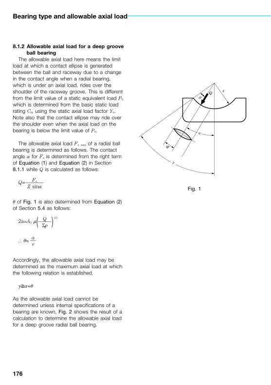
176


8.1.2 Allowable axial load for a deep groove 　　　ball bearing

The allowable axial load here means the limit load at which a contact ellipse is generated between the ball and raceway due to a change in the contact angle when a radial bearing, which is under an axial load, rides over the shoulder of the raceway groove. This is different from the limit value of a static equivalent load P0 which is determined from the basic static load rating C0r using the static axial load factor Y0. Note also that the contact ellipse may ride over the shoulder even when the axial load on the bearing is below the limit value of P0.

The allowable axial load Fa max of a radial ball bearing is determined as follows. The contact angle a for Fa is determined from the right term of Equation (1) and Equation (2) in Section 8.1.1 while Q is calculated as follows:

Q=

q of Fig. 1 is also determined from Equation (2) of Section 5.4 as follows:

2a=A2 m 1/3

\ q≒

Accordingly, the allowable axial load may be determined as the maximum axial load at which the following relation is established.

g≧a+q

As the allowable axial load cannot be determined unless internal specifications of a bearing are known, Fig. 2 shows the result of a calculation to determine the allowable axial load for a deep groove radial ball bearing.

Fa

Z sina

( )QSr

ar

Q r

a

θ

α

γ

Fig. 1

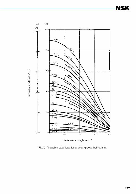
176 177

　　Fig. 2　Allowable axial load for a deep groove ball bearing

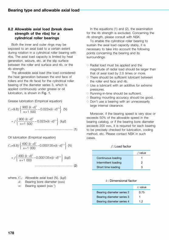
178


8.2 Allowable axial load (break down strength of the ribs) for a cylindrical roller bearings

Both the inner and outer rings may be exposed to an axial load to a certain extent during rotation in a cylindrical roller bearing with ribs. The axial load capacity is limited by heat generation, seizure, etc. at the slip surface between the roller end surface and rib, or the rib strength.

The allowable axial load (the load considered the heat generation between the end face of rollers and the rib face) for the cylindrical roller bearing of the diameter series 3, which is applied continuously under grease or oil lubrication, is shown in Fig. 1.

Grease lubrication (Empirical equation)

CA=9.8 f – 0.023´(k ·d)2.5 (N)

= f – 0.023´(k ·d)2.5 {kgf}

.......................................... (1)

Oil lubrication (Empirical equation)

CA=9.8 f –0.000135´(k ·d)3.4　 (N)

= f –0.000135´(k ·d)3.4 {kgf}

.......................................... (2)

where, CA: Allowable axial load (N), {kgf} d: Bearing bore diameter (mm) n: Bearing speed (min–1)

In the equations (1) and (2), the examination for the rib strength is excluded. Concerning the rib strength, please consult with NSK.

To enable the cylindrical roller bearing to sustain the axial load capacity stably, it is necessary to take into account the following points concerning the bearing and its surroundings.

○ Radial load must be applied and the magnitude of radial load should be larger than that of axial load by 2.5 times or more.

○ There should be sufficient lubricant between the roller end face and rib.

○ Use a lubricant with an additive for extreme pressures.

○ Running-in-time should be sufficient.○ Bearing mounting accuracy should be good.○ Don’t use a bearing with an unnecessarily

large internal clearance.

Moreover, if the bearing speed is very slow or exceeds 50% of the allowable speed in the bearing catalog, or if the bearing bore diameter exceeds 200 mm, it is required for each bearing to be precisely checked for lubrication, cooling method, etc. Please contact NSK in such cases.

900 (k ·d)2

n+1 500

490 (k ·d)2

n+1 000

490 (k ·d)2

n+1 000

900 (k ·d)2

n+1 500

f : Load factor

f value

Continuous loading

Intermittent loading

Short time loading

1

2

3

k : Dimensional factor

k value

Bearing diameter series 2



0.75

1

1.2

178 179

Fig. 1　Allowable axial load for a cylindrical roller bearing

180

9. Lubrication

9.1 Lubrication amount for the forced lubrication method

When a rolling bearing runs at high speed, the rolling friction of the bearing itself and the churning of lubricant cause heat generation, resulting in substantial temperature rise. Positive removal or dissipation of such generated heat serves greatly to prevent overheating in bearings. The maintenance of a sufficient lubrication oil film ensures stable and continuous operation of bearings at high speed.

Various heat removal or dissipation methods are available. An effective method is to remove the heat directly from bearings by forcing a large quantity of lubricating oil to circulate inside the bearing. This method is called the forced lubrication method. In this case, the amount of oil supplied is mostly determined on the basis of the actual operating conditions. Important factors to be considered include the allowable temperature of the machine or system, radiation effect, and heat generation caused by oil stirring.

Below is an empirical equation which can be used to estimate the amount of forced circulation oil needed for a bearing.

Q= d m n F (N) ................ (1)

= d m n F {kgf}

where, Q: Oil supply rate (liters/min) T1: Oil temperature at the oil inlet (°C) T2: Oil temperature at the oil outled (°C) d: Bearing bore (mm) m: Coefficient of dynamic friction

(Table 1) n: Bearing speed (min–1) F: Load on a bearing (N), {kgf}

Systems employing the forced circulation lubrication method include large industrial machinery, such as a paper making machines, presses, steel-making machines, and various speed reducers. Most of these machines incorporate a large bearing. As an example, the calculation of the supply rate for a spherical roller bearing used in a speed reducer is shown below:

Bearing: 22324 CAM E4 C3 d=120 mm m=0.0028Speed: n=1 800 min–1

Bearing load: F=73 500 N, {7 500 kgf}Temperature difference: Assumed to be T2–T1=20°C

Q≒ ×120×0.0028×1 800

　×73 500≒4.2

The calculated value is about 4 liters/min. This value is only a guideline and may be modified after considering such factors as restrictions on the oil supply and oil outlet bore.

Note that the oil drain pipe and oil drain port must be designed large enough to prevent stagnation of the circulating oil in the housing. For a large bearing with a bore exceeding 200 mm, which is exposed to a heavy load, the oil amount according to Equation (1) is calculated to be slightly larger. However, the user may select a value of about 1/2 to 2/3 of the above calculated value for most practical applications.

0.19×10–5

T2–T1

1.85×10–5

T2–T1

0.19×10–5

20

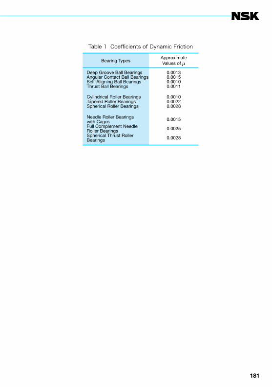
180 181

Table 1 Coefficients of Dynamic Friction

Bearing TypesApproximateValues of m

Deep Groove Ball BearingsAngular Contact Ball BearingsSelf-Aligning Ball BearingsThrust Ball Bearings

0.00130.00150.00100.0011

Cylindrical Roller BearingsTapered Roller BearingsSpherical Roller Bearings

0.00100.00220.0028

Needle Roller Bearingswith CagesFull Complement NeedleRoller BearingsSpherical Thrust RollerBearings

0.0015

0.0025

0.0028

182

Lubrication

9.2 Grease filling amount of spindle bearing for machine tools

Recent machine tools, such as machining centers and NC lathes, show a remarkable trend towards increased spindle speeds. The positive results of these higher speeds include enhanced machining efficiency and improved accuracy of the machined surface. But a problem has emerged in line with this trend. Faster spindle speeds cause the spindle temperature to rise which adversely affects the machining accuracy.

In general, grease lubrication is employed with spindle bearings and in particular, for spindle bearings with bores of 150 mm or less. When grease lubrication is employed, filling the bearing with too much grease may cause abnormal heat generation. This is an especially severe problem during the initial operation immediately after filling, and may even result in the deterioration of the grease. It is essential to prevent such a problem by taking sufficient time for a thorough warm-up. In other words, the spindle bearing needs to be accelerated gradually during its initial operation.

Based on its past experience, NSK recommends that spindle bearings for machine tools be filled with the standard amount of grease, which is equivalent to 10% of the cylindrical roller bearing free internal space or 15% of the angular contact ball bearing free internal space, so as to facilitate the initial warm-up wihtout adversely affecting the lubrication performance.

Table 1 shows the standard grease filling amount for bearings used in spindles which is equivalent to 10% of the bearing free space. As an alternative to this table, the simplified equation shown next may be used to estimate the value.

V10= f×10–5 (D2–d2) B

where, V10: Approximate filling amount (cm3) D: Nominal outside diameter (mm) d: Nominal bore (mm) B: Nominal bearing width (mm) f=1.5 for NN30 series and BA10X and 　BT10X series f=1.7 for 70 and 72 series f=1.4 for NN49 series

The grease for high-speed bearings should be a quality grease: use a grease with a synthetic oil as a base if the application involves ball bearings; use a grease with a mineral oil as a base if the application involves roller bearings.

182 183

Remarks　For the 　　TAC2OD double-direction angular-contact thrust ball bearings, grease should be filled to the same amount as that for the NN30 double-row cylindrical roller bearing.

Table 1 Standard grease filling amounts for spindle bearings for machine toolsUnits: cm3

Bearingbore No.

Bearingbore

dimension(mm)

Filling amount (per bearing)

Cylindrical roller bearing High-speed angular contact thrust ball

bearing BA, BT series

Angular contact ball bearing High-speed angular contact ball bearing

NN30 series N10B series 70 series 72 series BNC10 series

10

11

12

13

14

15

16

17

18

19

20

21

22

24

26

28

30

32

44

50

55

60

65

70

75

80

85

90

95

100

105

110

120

130

140

150

160

170

1.4

2.0

2.1

2.2

3.2

3.5

4.7

4.9

6.5

6.6

6.8

9.3

11

12.5

18

20

23

29

38

1.1

1.5

1.7

1.8

2.4

2.5

3.3

3.5

4.7

4.8

5.1

6.7

7.8

8.1

12.4

　

　

　

　

1.2

2.0

2.0

2.1

3.0

3.2

4.2

4.4

6.0

6.3

6.5

8.4

10.1

10.8

16.5

17.1

21.8

26.9

32.4

1.7

2.3

2.4

2.7

3.6

3.8

5.1

5.3

6.9

7.2

7.4

9.3

11.9

12.3

19.5

20.7

25.8

33.8

41.6

3.1

4.0

4.9

5.7

6.6

7.2

8.8

10.9

13.5

16.3

19.8

23.4

27.0

32.0

35.3

42.6

53.6

62.6

81.4

1.5

2.0

2.0

2.3

3.3

3.6

4.4

4.7

6.2

6.5

6.8

8.1

10.1

10.8

16.1

17.0

21.2

25.5

33.2

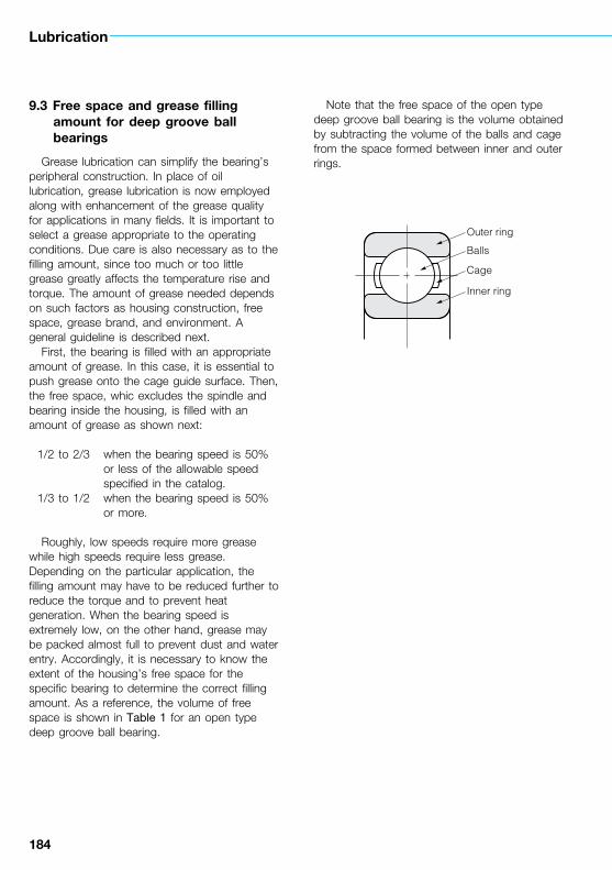
184

Lubrication

9.3 Free space and grease filling amount for deep groove ball bearings

Grease lubrication can simplify the bearing’s peripheral construction. In place of oil lubrication, grease lubrication is now employed along with enhancement of the grease quality for applications in many fields. It is important to select a grease appropriate to the operating conditions. Due care is also necessary as to the filling amount, since too much or too little grease greatly affects the temperature rise and torque. The amount of grease needed depends on such factors as housing construction, free space, grease brand, and environment. A general guideline is described next.

First, the bearing is filled with an appropriate amount of grease. In this case, it is essential to push grease onto the cage guide surface. Then, the free space, whic excludes the spindle and bearing inside the housing, is filled with an amount of grease as shown next:

1/2 to 2/3 when the bearing speed is 50% or less of the allowable speed specified in the catalog.

1/3 to 1/2 when the bearing speed is 50% or more.

Roughly, low speeds require more grease while high speeds require less grease. Depending on the particular application, the filling amount may have to be reduced further to reduce the torque and to prevent heat generation. When the bearing speed is extremely low, on the other hand, grease may be packed almost full to prevent dust and water entry. Accordingly, it is necessary to know the extent of the housing’s free space for the specific bearing to determine the correct filling amount. As a reference, the volume of free space is shown in Table 1 for an open type deep groove ball bearing.

Note that the free space of the open type deep groove ball bearing is the volume obtained by subtracting the volume of the balls and cage from the space formed between inner and outer rings.

Outer ring

Balls

Cage

Inner ring

184 185

Remarks　The table above shows the free space of a bearing using a pressed steel cage. The free space of a bearing using a high-tension brass machined cage is about 50 to 60% of the value in the table.

Table 1 Free space of open type deep groove ball bearingUnits: cm3

Bearingbore No.

Bearing free spaceBearingbore No.

Bearing free space

Bearing series Bearing series

60 62 63 60 62 63

00

01

02

03

04

05

06

07

08

09

10

11

12

13

1.2

1.2

1.6

2.0

4.0

4.6

6.5

9.2

11

14

15

22

23

24

1.5

2.1

2.7

3.7

6.0

7.7

11

15

20

23

28

34

45

54

2.9

3.5

4.8

6.4

7.9

12

19

25

35

49

64

79

98

122

14

15

16

17

18

19

20

21

22

24

26

28

30

32

34

35

47

48

63

66

68

88

114

122

172

180

220

285

61

67

84

104

127

155

184

216

224

310

355

415

485

545

148

180

213

253

297

345

425

475

555

675

830

1 030

1 140

1 410

186

Lubrication

9.4 Free space of angular contact ball bearings

Angular contact ball bearings are used in various components, such as spindles of machine tools, vertical pump motors, and worm gear reducers.

This kind of bearing is used mostly with grease lubrication. But such grease lubrication may affect the bearing in terms of temperature rise or durability. To allow a bearing to demonstrate its full performance, it is essential to fill the bearing with the proper amount of a suitable grease. A prerequisite for this job is a knowledge of the bearing’s free space.

The angular ball bearing is available in various kinds which are independent of the combinations of bearing series, contact angle, and cage type. The free space of the bearing used most frequently is described below. Table 1 shows the free space of a bearing with a pressed cage for general use and Table 2 shows that of a bearing with a high-tension brass machined cage. The contact angle symbols A, B, and C in each table refer to the nominal contact angle of 30°, 40°, and 15° of each bearing.

Table 1 Free space of angular contact ball bearing (1)

(with pressed steel cage) Units: cm3

Bearingbore No.

Bearing free space

Bearing series 　 Contact angle symbol

72-A 72-B 73-A 73-B

00

01

02

03

04

05

06

07

08

09

10

1.5

2.1

2.8

3.7

6.2

7.8

12

16

20

25

28

1.4

2.0

2.7

3.6

5.9

7.4

11

15

19

24

27

2.9

3.7

4.8

6.2

8.4

13

20

26

36

48

63

2.8

3.5

4.6

5.9

8.0

12

19

24

34

45

60

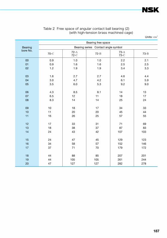
186 187

Table 2 Free space of angular contact ball bearing (2) (with high-tension brass machined cage)

Units: cm3

Bearingbore No.

Bearing free space

Bearing series 　 Contact angle symbol

70-C 72-A72-C 72-B 73-A

73-C 73-B

000102

030405

060708

091011

121314

151617

181920

0.90.91.2

1.63.03.5

4.36.58.3

101116

171824

243437

444447

1.01.61.9

2.74.76.0

8.51214

182026

333843

475871

88105127

1.01.61.9

2.74.25.3

8.11114

172025

313742

455770

85105127

2.22.53.4

4.66.19.2

141825

344557

7187

107

129152179

207261282

2.12.53.3

4.45.99.0

131724

334455

6983

103

123146172

201244278

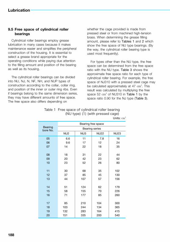
188

Lubrication

9.5 Free space of cylindrical roller bearings

Cylindrical roller bearings employ grease lubrication in many cases because it makes maintenance easier and simplifies the peripheral construction of the housing. It is essential to select a grease brand appropriate for the operating conditions while paying due attention to the filling amount and position of the bearing as well as its housing.

The cylindrical roller bearings can be divided into NU, NJ, N, NF, NH, and NUP types of construction according to the collar, collar ring, and position of the inner or outer ring ribs. Even if bearings belong to the same dimension series, they may have different amounts of free space. The free space also differs depending on

whether the cage provided is made from pressed steel or from machined high-tension brass. When determining the grease filling amount, please refer to Tables 1 and 2 which show the free space of NU type bearings. (By the way, the cylindrical roller bearing type is used most frequently).

For types other than the NU type, the free space can be determined from the free space ratio with the NU type. Table 3 shows the approximate free space ratio for each type of cylindrical roller bearing. For example, the free space of NJ310 with a pressed steel cage may be calculated approximately at 47 cm3. This result was calculated by multiplying the free space 52 cm3 of NU310 in Table 1 by the space ratio 0.90 for the NJ type (Table 3).

Table 1 Free space of cylindrical roller bearing (NU type) (1) (with pressed cage)

Units: cm3

Bearingbore No.

Bearing free space

Bearing series

NU2 NU3 NU22 NU23

050607

080910

111213

141516

17181920

6.69.6

14

182023

303744

515871

85103132151

11 17 22

31 42 52

68 85107

124155177

210244283335

7.81218

222326

354557

627085

104134164200

16 24 35

44 62 80

102130156

179226260

300365415540

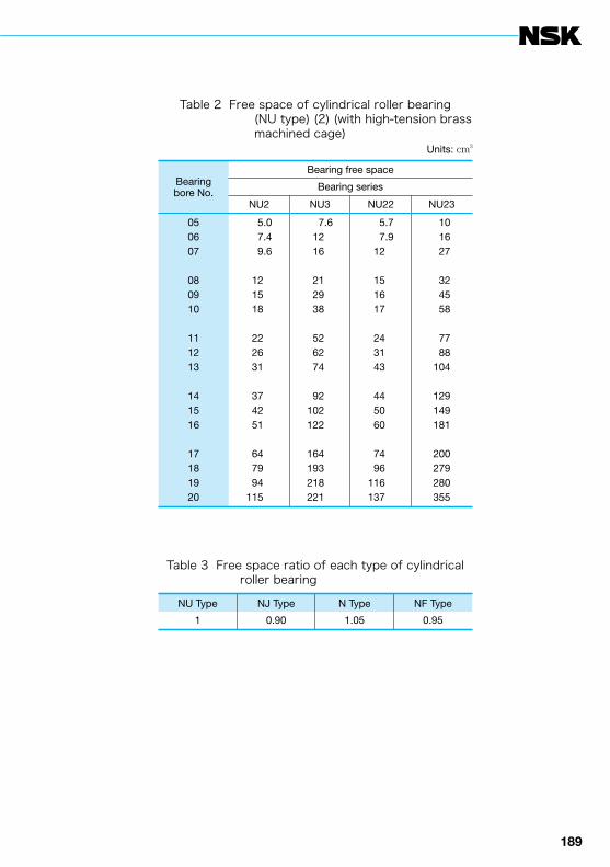
188 189

Table 2 Free space of cylindrical roller bearing (NU type) (2) (with high-tension brass machined cage)

Units: cm3

Bearingbore No.

Bearing free space

Bearing series

NU2 NU3 NU22 NU23

050607

080910

111213

141516

17181920

5.07.49.6

121518

222631

374251

647994

115

7.61216

212938

526274

92102122

164193218221

5.77.9

12

151617

243143

445060

7496

116137

10 16 27

32 45 58

77 88104

129149181

200279280355

Table 3 Free space ratio of each type of cylindrical roller bearing

NU Type NJ Type N Type NF Type

1 0.90 1.05 0.95

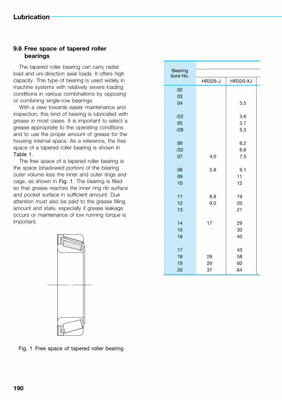
190

Lubrication

9.6 Free space of tapered roller bearings

The tapered roller bearing can carry radial load and uni-direction axial loads. It offers high capacity. This type of bearing is used widely in machine systems with relatively severe loading conditions in various combinations by opposing or combining single-row bearings.

With a view towards easier maintenance and inspection, this kind of bearing is lubricated with grease in most cases. It is important to select a grease appropriate to the operating conditions and to use the proper amount of grease for the housing internal space. As a reference, the free space of a tapered roller bearing is shown in Table 1.

The free space of a tapered roller bearing is the space (shadowed portion) of the bearing outer volume less the inner and outer rings and cage, as shown in Fig. 1. The bearing is filled so that grease reaches the inner ring rib surface and pocket surface in sufficient amount. Due attention must also be paid to the grease filling amount and state, especially if grease leakage occurs or maintenance of low running torque is important.

Fig. 1　Free space of tapered roller bearing

Bearingbore No.

HR329-J HR320-XJ

020304

/2205/28

06/3207

080910

111213

141516

17181920

　　　

　　　

　　4.0

5.8　　

8.89.0　

17　　

　282937

　　3.5

3.63.75.3

6.26.67.5

9.11112

192021

293040

43586064

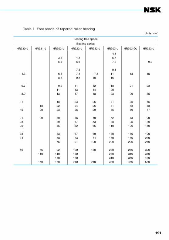
190 191

Table 1 Free space of tapered roller bearingUnits: cm3

Bearing free space

Bearing series

HR330-J HR331-J HR302-J HR322-J HR332-J HR303-J HR303-DJ HR323-J

　　　

　4.3　

6.7　8.9

11　

15

212325

3334

　

49　　　

　　　

　　　

　　　

　 18 20

29　　

　　　

76110

　150

　3.35.3

　6.38.8

9.21113

182223

303945

535875

92110140160

　4.36.6

7.37.49.8

111317

232426

364762

677391

120150170210

　　　

　7.5

10

121418

252629

405365

6974

100

130　　

240

4.55.77.2

9.11116

182023

314155

7288

110

130160200

230260310380

　　　

　 13

　

21　

26

35 48 59

78 95120

150180200

250310350460

　　9.2

　15　

23　

35

455877

99130150

190230270

320370430580

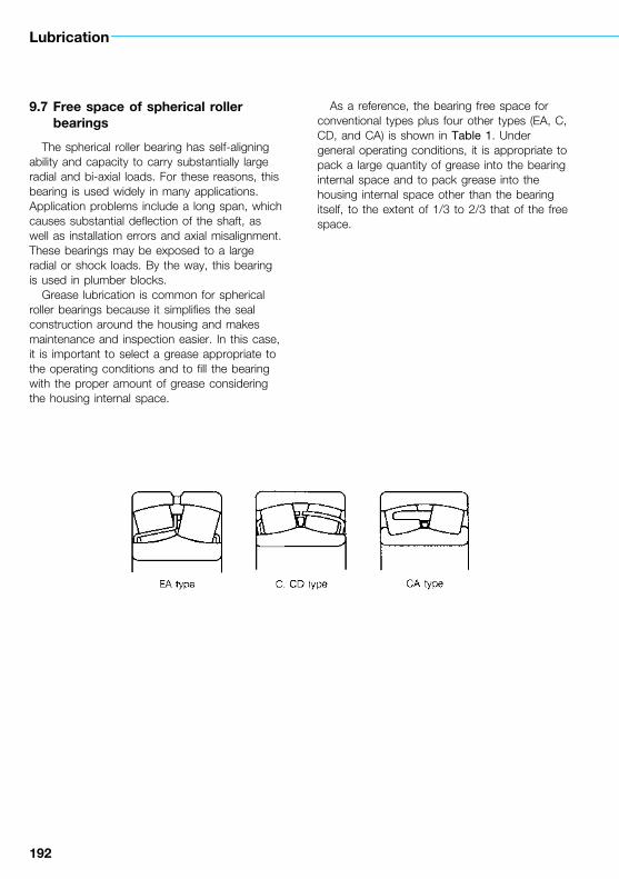
192

Lubrication

9.7 Free space of spherical roller bearings

The spherical roller bearing has self-aligning ability and capacity to carry substantially large radial and bi-axial loads. For these reasons, this bearing is used widely in many applications. Application problems include a long span, which causes substantial deflection of the shaft, as well as installation errors and axial misalignment. These bearings may be exposed to a large radial or shock loads. By the way, this bearing is used in plumber blocks.

Grease lubrication is common for spherical roller bearings because it simplifies the seal construction around the housing and makes maintenance and inspection easier. In this case, it is important to select a grease appropriate to the operating conditions and to fill the bearing with the proper amount of grease considering the housing internal space.

As a reference, the bearing free space for conventional types plus four other types (EA, C, CD, and CA) is shown in Table 1. Under general operating conditions, it is appropriate to pack a large quantity of grease into the bearing internal space and to pack grease into the housing internal space other than the bearing itself, to the extent of 1/3 to 2/3 that of the free space.

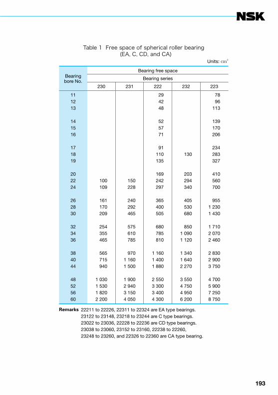
192 193

Table 1 Free space of spherical roller bearing (EA, C, CD, and CA)

Units: cm3

Bearingbore No.

Bearing free space

Bearing series

230 231 222 232 223

111213

141516

171819

202224

262830

323436

384044

48525660

　　　

　　　

　　　

　 100 109

161 170 209

254 355 465

565 715 940

1 0301 5301 8202 200

　　　

　　　

　　　

　 150 228

240 292 465

575 610 785

9701 1601 500

1 9002 9403 1504 050

29 42 48

52 57 71

91 110 135

169 242 297

365 400 505

680 785 810

1 1601 4001 880

2 5503 3003 4004 300

　　　

　　　

　 130

　

203 294 340

405 530 680

8501 0901 120

1 3401 6402 270

3 5504 7504 9506 200

78 96 113

139 170 206

234 283 327

410 560 700

9551 2301 430

1 7102 0702 460

2 8302 9003 750

4 7005 9007 2508 750

Remarks 22211 to 22226, 22311 to 22324 are EA type bearings.23122 to 23148, 23218 to 23244 are C type bearings.23022 to 23036, 22228 to 22236 are CD type bearings.23038 to 23060, 23152 to 23160, 22238 to 22260,23248 to 23260, and 22326 to 22360 are CA type bearing.

194

Lubrication

9.8 NSK’s dedicated greases

9.8.1 NS7 and NSC greases for induction motor bearings

NS7 and NSC greases have been developed by NSK mainly for lubrication of bearings for induction motors. These greases consist of ingredients such as synthetic oil and lithium soap. Synthetic oil is superior in oxidation, thermal stability, and low-temperature fluidity while lithium soap is superior in water resistance, and shearing stability.

NS7 and NSC greases are applicable over a wide range of temperature from –40°C to +140°C. The viscosity of the base oil is lowest in NS7 and highest in NSC. Namely, NS7 grease is best suited when the low-temperature performance is important and NSC grease for high-temperature performance.

Features(1) Superior in high-temperature durability, with

long grease life(2) Superior in low-temperature performance,

with less abnormal sound and vibration in a bearing at cold start

(3) Superior in high-speed running performance, with little grease leakage

(4) Reduction of the friction torque of a bearing at low and room temperature

(5) Fewer particle inclusions and satisfactory acoustic performance. Moreover, NSC grease can maintain superior acoustic performance over a long period (long acoustic life).

(6) Superior in water resistance(7) Superior in anti-rusting performance against

salt water

Table 1 Characteristics of NS7 and NSC greases

Characteristics NS7 NSC Test method

Appearance

Thickener

Base oil

Kinematic viscosity of base oil, mm2/s　　 40°C　　 100°C

Worked penetration, 25°C, 60W

Dropping point, °C

Corrosiveness, (Copper strip) 100°C, 24 h

Evaporation, %　99°C, 22 h

Oil separation, %　100°C, 24 h

Oxidative stability, kPa　99°C, 100 h

Worked stability, 25°C, 105W

Water wash-out, %　38°C, 1 h

Low temperature torque, mN　m　−30°C　　 Starting {−40°C}　　 Running

Rust protection test, 0.1%, NaCl25°C, 48 h, 100% RH

Light brown

Li soap

Polyolesterdiester

26.05.0

250

192

Good

0.30

1.2

25

306

1.4

{115}{25}

1,1,1

Light brown

Li soap

Polyolester diphenylether

53.08.3

235

192

Good

0.25

1.1

20

332

1.4

42184

1,1,1

　

　

　

JIS K 2283

JIS K 2220: 2003 (Clause 7)

JIS K 2220: 2003 (Clause 8)

JIS K 2220: 2003 (Clause 9)

JIS K 2220: 2003 (Clause 10)

JIS K 2220: 2003 (Clause 11)

JIS K 2220: 2003 (Clause 12)

JIS K 2220: 2003 (Clause 15)

JIS K 2220: 2003 (Clause 16)

JIS K 2220: 2003 (Clause 18)

ASTM D 1743

Remarks　The value of parentheses is low temperature torque value at −40　.

194 195

Application* Motor for home electric products (video

cassette recorder, air conditioner fan motor, electric oven hood fan motor)

* Motor for office automation equipment (fixed disk drive spindle, floppy disk drive spindle, stepping motor, IC cooling fan motor)

* Industrial motor (blower motor, pump motor, large and medium motor)

* Automotive equipment (starter, distributor, wind shield wiper motor)

Fig. 1　Grease life

Fig. 2　Acoustic life

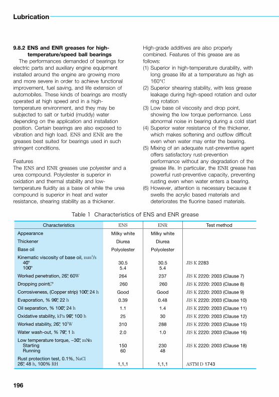
196

Lubrication

9.8.2 ENS and ENR greases for high-temperature/speed ball bearings

The performances demanded of bearings for electric parts and auxiliary engine equipment installed around the engine are growing more and more severe in order to achieve functional improvement, fuel saving, and life extension of automobiles. These kinds of bearings are mostly operated at high speed and in a high-temperature environment, and they may be subjected to salt or turbid (muddy) water depending on the application and installation position. Certain bearings are also exposed to vibration and high load. ENS and ENR are the greases best suited for bearings used in such stringent conditions.

FeaturesThe ENS and ENR greases use polyester and a urea compound. Polyolester is superior in oxidation and thermal stability and low-temperature fluidity as a base oil while the urea compound is superior in heat and water resistance, shearing stability as a thickener.

High-grade additives are also properly combined. Features of this grease are as follows:(1) Superior in high-temperature durability, with

long grease life at a temperature as high as 160°C

(2) Superior shearing stability, with less grease leakage during high-speed rotation and outer ring rotation

(3) Low base oil viscosity and drop point, showing the low torque performance. Less abnormal noise in bearing during a cold start

(4) Superior water resistance of the thickener, which makes softening and outflow difficult even when water may enter the bearing.

(5) Mixing of an adequate rust-preventive agent offers satisfactory rust-prevention performance without any degradation of the grease life. In particular, the ENR grease has powerful rust-preventive capacity, preventing rusting even when water enters a bearing.

(6) However, attention is necessary because it swells the acrylic based materials and deteriorates the fluorine based materials.

Table 1 Characteristics of ENS and ENR grease

Characteristics ENS ENR Test method

Appearance

Thickener

Base oil



Dropping point, °C







Low temperature torque, −30°C, mN　m　　 Starting　　 Running


Milky white

Diurea

Polyolester

30.55.4

264

　260

Good

0.39

1.1

25

310

2.0

15060

1,1,1

Milky white

Diurea

Polyolester

30.55.4

237

　260

Good

0.48

1.4

30

288

1.0

23048

1,1,1

　

　

　

JIS K 2283

JIS K 2220: 2003 (Clause 7)

JIS K 2220: 2003 (Clause 8)

JIS K 2220: 2003 (Clause 9)

JIS K 2220: 2003 (Clause 10)

JIS K 2220: 2003 (Clause 11)

JIS K 2220: 2003 (Clause 12)

JIS K 2220: 2003 (Clause 15)

JIS K 2220: 2003 (Clause 16)

JIS K 2220: 2003 (Clause 18)

ASTM D 1743

196 197

Applications* Electric equipment (electromagnetic clutch,

alternator, starter, idler pulley)* Engine auxiliary equipment (timing belt

tensioner, clutch release)

* Office automation equipment (copying machine heat roller)

* Motors (inverter motor, servo motor)


Test method　As per ASTM D 1743　　Bearing: Tapered roller bearing 09074R/09194R (φ19.05×φ49.23×23.02 mm)　　Relative humidioy: 100 %Evaluation:　1; No rusting, 2; Minor rusting in three or less points, 3; Worse than Rank 2

Table 2 Bearing rust-prevention test

Base oilthickener

Testconditions

ENSTable 1

ENRTable 1

Wide range grease High-temp grease

Ester syntheticoil

Ester syntheticoil and mineral

oilMineral oil Mineral oil

Table 1 Table 1 Li soap Naterephtalamate

Li complexsoap Polyurea

0.1% salt 25°C, 48 h

0.5% salt 52°C, 24 h

1.0% salt 52°C, 24 h

1,1,1

2,2,3

　

1,1,1

1,1,1

1,1,1

1,1,1

1,2,2

　

1,1,1

1,1,1

1,2,2

3,3,3

　

　

1,1,1

1,2,2

　

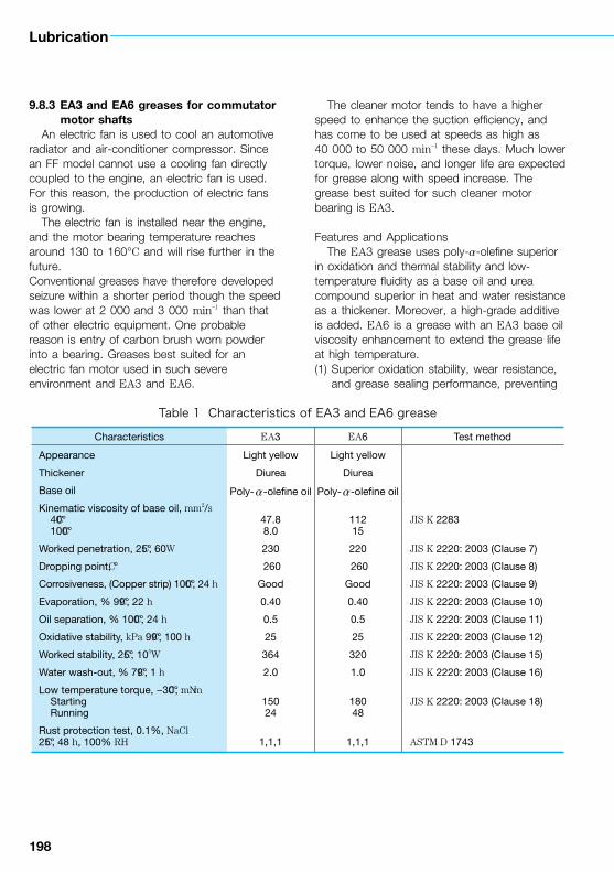
198

Lubrication

9.8.3 EA3 and EA6 greases for commutator motor shafts

An electric fan is used to cool an automotive radiator and air-conditioner compressor. Since an FF model cannot use a cooling fan directly coupled to the engine, an electric fan is used. For this reason, the production of electric fans is growing.

The electric fan is installed near the engine, and the motor bearing temperature reaches around 130 to 160°C and will rise further in the future.Conventional greases have therefore developed seizure within a shorter period though the speed was lower at 2 000 and 3 000 min–1 than that of other electric equipment. One probable reason is entry of carbon brush worn powder into a bearing. Greases best suited for an electric fan motor used in such severe environment and EA3 and EA6.

The cleaner motor tends to have a higher speed to enhance the suction efficiency, and has come to be used at speeds as high as 40 000 to 50 000 min–1 these days. Much lower torque, lower noise, and longer life are expected for grease along with speed increase. The grease best suited for such cleaner motor bearing is EA3.

Features and ApplicationsThe EA3 grease uses poly-a-olefine superior

in oxidation and thermal stability and low-temperature fluidity as a base oil and urea compound superior in heat and water resistance as a thickener. Moreover, a high-grade additive is added. EA6 is a grease with an EA3 base oil viscosity enhancement to extend the grease life at high temperature.(1) Superior oxidation stability, wear resistance,

and grease sealing performance, preventing

Table 1 Characteristics of EA3 and EA6 grease

Characteristics EA3 EA6 Test method

Appearance

Thickener

Base oil



Dropping point, °C









Light yellow

Diurea

Poly-a-olefine oil

47.88.0

230

　260

Good

0.40

0.5

25

364

2.0

15024

1,1,1

Light yellow

Diurea

Poly-a-olefine oil

11215

220

　260

Good

0.40

0.5

25

320

1.0

18048

1,1,1

　

　

　

JIS K 2283

JIS K 2220: 2003 (Clause 7)

JIS K 2220: 2003 (Clause 8)

JIS K 2220: 2003 (Clause 9)

JIS K 2220: 2003 (Clause 10)

JIS K 2220: 2003 (Clause 11)

JIS K 2220: 2003 (Clause 12)

JIS K 2220: 2003 (Clause 15)

JIS K 2220: 2003 (Clause 16)

JIS K 2220: 2003 (Clause 18)

ASTM D 1743

198 199

entry of carbon brush abrasion powder into a bearing. The grease life in the electric fan motor bearing is long. EA3 is suitable when low-torque performance is important and EA6 is suitable when the bearing temperature exceeds 150°C.

(2) EA3 grease is superior in low-torque and low-noise performances, with superior fluidity, showing superb lubrication performance during rotation as fast as 40 000 to 50 000 min–1. Also, the grease life of a cleaner motor bearing is longer.

(3) Superior rust-preventive performance and less adverse effect on rubber and plastics.

(4) However, attention is necessary because it deteriorates the fluorine based materials.

Fig. 1　Durability test with electric fan motors

Fig. 2　Running torque


200

Lubrication

9.8.4 WPH grease for water pump bearingsAn automotive water pump is a pump to

circulate cooling water through the engine. A typical bearing for a water pump is a bearing unit which measures 16 mm in shaft diameter and 30 mm in outer shell diameter and uses either balls with balls or balls with rollers. Though the water pump bearing unit is equipped with a high-performance seal, cooling water may enter the unit. In fact, most water pump bearing failures can be attributed to entry of coolant into the bearing.

Recently, the bearing speed tends to rise in line with performance and efficiency enhancement of engines. Moreover, the bearing temperature rises further along with temperature rise of the cooling water and engine. The bearing load is also growing these days as the number of models employing poly V-belts is growing rapidly.

The grease guaranteeing high reliability and best applicability for water pump bearings and bearing units used in such severe environment is WPH.

FeaturesThe WPH grease uses poly-a-olefine, which is

superior in oxidation and thermal stability, as a base oil and a urea compound, which is superior in heat and water resistance, as a thickener. A high-grade additive is also used. Features are as described below:(1) This grease does not readily soften and

outflow even if coolant enters the bearing. Also, this grease can maintain satisfactory lubrication performance over an extended period of time. As a result, this grease can prevent flaking in a bearing.

(2) Superior in high-temperature durability, preventing deterioration and seizure even when the bearing temperature rises.

(3) Superior rust-preventive performance prevents rusting even if water or coolant enters the bearing.

Table 1 Characteristics of WPH grease

Characteristics WPH Test method

Appearance

Thickener

Base oil



Dropping point,°C









Butter-like milky yellow

Diurea

Poly-a-olefine oil

95.814.4

240

259

Good

0.20

0.2

20

306

0

24045

1,1,1

　

　

　

JIS K 2283

JIS K 2220: 2003 (Clause 7)

JIS K 2220: 2003 (Clause 8)

JIS K 2220: 2003 (Clause 9)

JIS K 2220: 2003 (Clause 10)

JIS K 2220: 2003 (Clause 11)

JIS K 2220: 2003 (Clause 12)

JIS K 2220: 2003 (Clause 15)

JIS K 2220: 2003 (Clause 16)

JIS K 2220: 2003 (Clause 18)

ASTM D 1743

200 201

Fig. 1　Water resistant test of grease for water pump bearings

Fig. 2　Life test of water pump bearings

202

Lubrication

9.8.5 MA7 and MA8 greases for automotive electric accessory bearings

Severe performance criteria for automotive electric accessory or engine auxiliary equipment bearings are increasingly requested to meet the high-capability, fuel saving, and long-life requirements of cars. These bearings are located in narrow engine compartments, which generally provide a hot environment. Furthermore, the adoption of poly-V-belts, which have excellent endurance, results in constantly

high loads on the bearings. Also, depending on the conditions, salty or muddy water may enter the bearings. MA7 and MA8 greases are the optimum greases for use in bearings which run under such severe operating conditions.

Table 1 Characteristics of MA7 and MA8 grease

Characteristics MA7 MA8 Test method

Appearance

Thickener

Base oil



Dropping point, °C









Light brown

Diurea

Ether-basesynthetic oil

10313

290

248

Good

0.18

0.6

20

335

1.0

304206

1,1,1

Milky white

Diurea

Ether-basesynthetic

hydrocarbon oil

7611

277

　260

Good

0.39

0.6

125

330

1.0

28057

1,1,1

　

　

　

JIS K 2283

JIS K 2220: 2003 (Clause 7)

JIS K 2220: 2003 (Clause 8)

JIS K 2220: 2003 (Clause 9)

JIS K 2220: 2003 (Clause 10)

JIS K 2220: 2003 (Clause 11)

JIS K 2220: 2003 (Clause 12)

JIS K 2220: 2003 (Clause 15)

JIS K 2220: 2003 (Clause 16)

JIS K 2220: 2003 (Clause 18)

ASTM D 1743

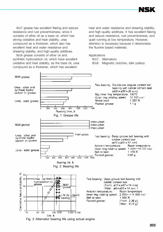
202 203

MA7 grease has excellent flaking and seizure resistance and rust preventiveness, since it consists of ether oil as a base oil, which has strong oxidative and heat stability, urea compound as a thickener, which also has excellent heat and water resistance and shearing stability, and high-quality additives.

MA8 grease consists of ether oil and synthetic hydrocarbon oil, which have excellent oxidative and heat stability, as the base oil, urea compound as a thickener, which has excellent

heat and water resistance and shearing stability, and high-quality additives. It has excellent flaking and seizure resistance, rust preventiveness, and quiet running at low temperature. However, attention is necessary because it deteriorates the fluorine based materials.

ApplicationsMA7: AlternatorsMA8: Magnetic clutches, idler pulleys


Fig. 2　Bearing life

Fig. 3　Alternator bearing life using actual engine

204

10. Bearing materials

10.1 Comparison of national standards of rolling bearing steel

The dimension series of rolling bearings as mechanical elements have been standardized internationally, and the material to be used for them specified in ISO 683/17 (heat treatment, alloy, and free cutting steels / Part 17 ball and roller bearing steels). However, materials are also standardized according to standards of individual countries and, in some cases, makers are even making their own modifications.

As internationalization of products incorporating bearings and references to the standards of these kinds of steels are increasing nowadays, applicable standards are compared and their features described for some representative bearing steels.

Notes　*1: P≦0.025, S≦0.025Remarks　ASTM: Standard of American Society

Table 1

JISG 4805 ASTM Other major

national standards

SUJ1 ≦ ≦

≦ 51100 ≦

SUJ2 ≦ ≦

≦ A 295-8952100

≦

≦ ≦ 100Cr6 (DIN)

≦ ≦ 100C6 (NF)

≦ ≦ 535A99 (BS)

SUJ3 ≦ ≦

≦ A 485-03Grade 1

≦

≦ A 485-03Grade 2

≦

SUJ4 ≦ ≦

SUJ5 ≦ ≦

≦ A 485-03Grade 3

≦

Notes　*2: P≦0.030, S≦0.030≦*3: P≦0.025, S≦0.015

JISG 4052G 4053

ASTMA 534-90 C

SCr420H

≦

≦

5120H

0.17 to 0.23

0.17 to 0.23

SCM420H

≦

≦

4118H

0.17 to 0.23

0.17 to 0.23

SNCM220H

≦

≦

8620H

0.17 to 0.23

0.17 to 0.23

SNCM420H

≦

≦

4320H

0.17 to 0.23

0.17 to 0.23

SNCM815

≦

≦

9310H

0.12 to 0.18

0.07 to 0.13

204 205

of Testing Materials, DIN: German Standard, NF: French Standard, BS: British Standard

Applicable national standards and chemical composition of high-carbon chrome bearing steel

Chemical composition (%)Application Remarks

C Si Mn Cr Mo Others

0.95 to 1.10 0.15 to 0.35 ≦0.50 0.90 to 1.20 ≦ *1 Not used generally

Equivalent to each other though there are slight differences in the ranges.

0.98 to 1.10 0.15 to 0.35 0.25 to 0.45 0.90 to 1.15 ≦0.10 *1

0.95 to 1.10 0.15 to 0.35 ≦0.50 1.30 to 1.60 ≦ *1 Typical steel type for small and medium size bearings

Equivalent to each other though there are slight differences in the ranges.

0.93 to 1.05 0.15 to 0.35 0.25 to 0.45 1.35 to 1.60 ≦0.10 P≦0.025S≦0.015

0.90 to 1.05 0.15 to 0.35 0.25 to 0.40 1.40 to 1.65 ≦ ≦

0.95 to 1.10 0.15 to 0.35 0.20 to 0.40 1.35 to 1.60 ≦0.08 P≦0.030S≦0.025

0.95 to 1.10 0.10 to 0.35 0.40 to 0.70 1.20 to 1.60 ≦ *1

0.95 to 1.10 0.40 to 0.70 0.90 to 1.15 0.90 to 1.20 ≦ *1 For large size bearings

SUJ3 is equivalent to Grade 1.Grade 2 hasbetter quenching capability

0.90 to 1.05 0.45 to 0.75 0.90 to 1.20 0.90 to 1.20 ≦0.10 P≦0.025S≦0.015

0.85 to 1.00 0.50 to 0.80 1.40 to 1.70 1.40 to 1.80 ≦0.10 P≦0.025S≦0.015

0.95 to 1.10 0.15 to 0.35 ≦0.50 1.30 to 1.60 0.10 to 0.25 *1 Scarcely used Better quenching capability than SUJ2

0.95 to 1.10 0.40 to 0.70 0.90 to 1.15 0.90 to 1.20 0.10 to 0.25 *1 For ultralarge size bearings

Though Grade 3 is equivalent to SUJ5, quenching capability of Grade 3 is better than SUJ5.

0.95 to 1.10 0.15 to 0.35 0.65 to 0.90 1.10 to 1.50 0.20 to 0.30 P≦0.025S≦0.015

Table 2 JIS and ASTM standards and chemical composition of carburizing bearing steel

Chemical composition (%)Application Remarks

Si Mn Ni Cr Mo Others

0.15 to 0.35

0.15 to 0.35

0.55 to 0.95

0.60 to 1.00

≦0.25

≦

0.85 to 1.25

0.60 to 1.00

≦

≦

*2

*3

For small bearings

Similar steel type

0.15 to 0.35

0.15 to 0.35

0.55 to 0.95

0.60 to 1.00

≦0.25

≦

0.85 to 1.25

0.30 to 0.70

0.15 to 0.35

0.08 to 0.15

*2

*3

For small bearings

Similar steel type, though quenching capability of 4118H is inferior to SCM420H

0.15 to 0.35

0.15 to 0.35

0.60 to 0.95

0.60 to 0.95

0.35 to 0.75

0.35 to 0.75

0.35 to 0.65

0.35 to 0.65

0.15 to 0.30

0.15 to 0.25

*2

*3

For small bearings

Equivalent, though there are slight differences

0.15 to 0.35

0.15 to 0.35

0.40 to 0.70

0.40 to 0.70

1.55 to 2.00

1.55 to 2.00

0.35 to 0.65

0.35 to 0.65

0.15 to 0.30

0.20 to 0.30

*2

*3

For medium bearings

Equivalent, though there are slight differences

0.15 to 0.35

0.15 to 0.35

0.30 to 0.60

0.40 to 0.70

4.00 to 4.50

2.95 to 3.55

0.70 to 1.00

1.00 to 1.45

0.15 to 0.30

0.08 to 0.15

*2

*3

For large bearings

Similar steel type

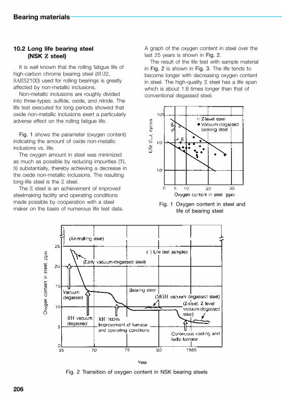
206

Bearing materials

10.2 Long life bearing steel (NSK Z steel)

It is well known that the rolling fatigue life of high-carbon chrome bearing steel (SUJ2, SAE52100) used for rolling bearings is greatly affected by non-metallic inclusions.

Non-metallic inclusions are roughly divided into three-types: sulfide, oxide, and nitride. The life test executed for long periods showed that oxide non-metallic inclusions exert a particularly adverse effect on the rolling fatigue life.

Fig. 1 shows the parameter (oxygen content) indicating the amount of oxide non-metallic inclusions vs. life.

The oxygen amount in steel was minimized as much as possible by reducing impurities (Ti, S) substantially, thereby achieving a decrease in the oxide non-metallic inclusions. The resulting long-life steel is the Z steel.

The Z steel is an achievement of improved steelmaking facility and operating conditions made possible by cooperation with a steel maker on the basis of numerous life test data.

A graph of the oxygen content in steel over the last 25 years is shown in Fig. 2.

The result of the life test with sample material in Fig. 2 is shown in Fig. 3. The life tends to become longer with decreasing oxygen content in steel. The high-quality Z steel has a life span which is about 1.8 times longer than that of conventional degassed steel.

Fig. 2　Transition of oxygen content in NSK bearing steels

Fig. 1　Oxygen content in steel and life of bearing steel

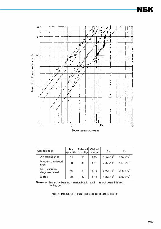
206 207

Fig. 3　Result of thrust life test of bearing steel

Remarks　Testing of bearings marked dark ≦ and ≦ has not been finished testing yet.

Classification Test quantity

Failured quantity

Weibull slope L10 L50

≦ Air-melting steel 44 44 1.02 1.67×106 1.06×107

≦ Vacuum degassed steel 30 30 1.10 2.82×106 1.55×107

≦ MGH vacuum degassed steel 46 41 1.16 6.92×106 3.47×107

≦ Z steel 70 39 1.11 1.26×107 6.89×107

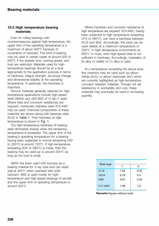
208

Bearing materials

10.3 High temperature bearing materials

Even for rolling bearings with countermeasures against high-temperature, the upper limit of the operating temperature is a maximum of about 400°C because of constraints of lubricant. This kind of bearing may be used in certain cases at around 500 to 600°C if the durable time, running speed, and load are restricted. Materials used for high-temperature bearings should be at a level appropriate to the application purpose in terms of hardness, fatigue strength, structural change, and dimensional stability at the operating temperature. In particular, the hardness is important.

Ferrous materials generally selected for high temperature applications include high-speed steel (SKH4) and AISI M50 of Cr-Mo-V steel. Where heat and corrosion resistances are required, martensitic stainless steel SUS　440C may be used. Chemical components of these materials are shown along with bearings steel SUJ2 in Table 1. Their hardness at high temperature is shown in Fig. 1.

The high-temperature hardness of bearing steel diminishes sharply when the tempering temperature is exceeded. The upper limit of the bearing’s operating temperature for a bearing having been subjected to normal tempering (160 to 200°C) is around 120°C. If high-temperature tempering (230 to 280°C) is made, then the bearing may be used up to around 200°C as long as the load is small.

SKH4 has been used with success as a bearing material for X-ray tube and can resist well at 450°C when operated with solid lubricant. M50 is used mostly for high-temperature and high-speed bearings of aircraft, and the upper limit of operating temperature is around 320°C.

Where hardness and corrosion resistance at high temperature are required, SUS　440C, having been subjected to high temperature tempering (470 to 480°C), can have a hardness between SUJ2 and M50. Accordingly, this steel can be used reliably at a maximum temperature of 200°C. In high temperature environments at 600°C or more, even high-speed steel is not sufficient in hardness. Accordingly, hastealloy of Ni alloy or stellite of Co alloy is used.

At a temperature exceeding the above level, fine ceramics may be used such as silicon nitride (Si3N4) or silicon carbonate (SiC) which are currently highlighted as high-temperature corrosion resistant materials. Though not yet satisfactory in workability and cost, these materials may eventually be used in increasing quantity.

Remarks≦Figures without≦mark

Steel typeC Si

SUJ2

SKH4

M50

SUS 440C

1.02

0.78

0.81

1.08

0.25

≦0.4

≦0.25

≦1.0

208 209

indicate median of tolerance.

Table 1 High-temperature bearing materials

Chemical composition %Remarks

Mn Ni Cr Mo W V Co

≦0.5

≦0.4

≦0.35

≦1.0

≦

≦

≦0.10

≦0.60

1.45

4.15

4.0

17.0

≦

≦

4.25

≦0.75

≦

18.0

≦0.25

≦

≦

1.25

1.0

≦

≦

10.0

≦0.25

≦

General use

High-temperatureuse

C o r r o s i o n resistance/high temperature

Fig. 1　Hardness of high-temperature materials

210

Bearing materials

10.4 Dimensional stability of bearing steel

Sectional changes or changes in the dimensions of rolling bearings as time passes during operation is called aging deformation. When the inner ring develops expansion due to such deformation, the result is a decrease in the interference between the shaft and inner ring. This becomes one of the causes of inner ring creep. Creep phenomenon, by which the shaft and inner ring slip mutually, causes the bearing to proceed from heat generation to seizure, resulting in critical damage to the entire machine. Consequently, appropriate measures must be taken against aging deformation of the bearing depending on the application.

Aging deformation of bearings may be attributed to secular thermal decomposition of retained austenite in steel after heat treatment. The bearing develops gradual expansion along with phase transformation.

The dimensional stability of the bearings, therefore, varies in accordance with the relative relationship between the tempering during heat treatment and the bearing’s operating temperature. The bearing dimensional stability increases with rising tempering temperature while the retained austenite decomposition gradually expands as the bearing’s operating temperature rises.

Fig. 1 shows how temperature influences the bearing’s dimensional stability. In the right-hand portion of the figure, the interference between the inner ring and shaft in various shaft tolerance classes is shown as percentages for the shaft diameter. As is evident from Fig. 1, the bearing dimensional stability becomes more unfavorable as the bearing’s temperature rises. Under these conditions, the interference between the shaft and inner ring of a general bearing is expected to decrease gradually. In this view, loosening of the fit surface needs to be prevented by using a bearing which has received dimension stabilization treatment.

Fig. 1　Bearing temperature and dimensional change ratio

210 211

When the bearing temperature is high, there is a possibility of inner ring creep. Since due attention is necessary for selection of an appropriate bearing, it is essential to consult NSK beforehand.

212

Bearing materials

10.5 Characteristics of bearing and shaft/housing materials

Rolling bearings must be able to resist high load, run at high speed, and endure long-time operation. It is also important to know the characteristics of the shaft and housing materials if the bearing performance is to be fully exploited. Physical and mechanical properties or typical materials of a bearing and shaft/housing are shown for reference in Table 1.

Note　 * JIS standard or reference value. ** Though Rockwell C scale is generallyRemarks　Proportional limits of SUJ2 and

Hou

sing

Bea

ring

Sha

ft

Material Heat treatment

SUJ2 Quenching, tempering

SUJ2 Spheroidizing annealing

SCr420 Quenching, low temptempering

SAE4320(SNCM420)

Quenching, low temptempering

SNCM815 Quenching, low temptempering

SUS440C Quenching, low temptempering

SPCC Annealing

S25C Annealing

CAC301(HBsC1) ≦≦

S45C Quenching, 650°Ctempering

SCr430 Quenching, 520 to 620°Cfast cooling

SCr440 Quenching, 520 to 620°Cfast cooling

SCM420 Quenching, 150 to 200°Cair cooling

SNCM439 Quenching, 650°Ctempering

SC46 Normalizing

SUS420J2 1 038°C oil cooling,400°C air cooling

FC200 Casting

FCD400 Casting

A1100 Annealing

AC4C Casting

ADC10 Casting

SUS304 Annealing

212 213

used, Brinel hardness is shown for comparison.SCr420 are 833 MPa {85 kgf/mm2} and 440 MPa {45 kgf/mm2} respectively as reference.

Table 1 Physical and mechanical properties of bearing and shaft/housing materials

Densityg/cm

Specificheat

kJ/(kg≦K)

Thermalconduc-

tivityW/(m≦K)

Electric resistanceμΩ≦cm

Linearexpansion

coeff.(0 to 100°C)×10−6/°C

Young,s

modulusMPa

{kgf/mm2}

Yield pointMPa

{kgf/mm2}

Tensilestrength

MPa{kgf/mm2}

Elong-ation

%

Hardness

HBRemarks

High carbonchromebearingsteel No. 2

ChromesteelNickelchromemolybde-num steelMartensiticstainlesssteelCold rolledsteel plateC a r b o n steelfor machinestructureH i g h -tensionbrassC a r b o n steelfor machinestructure

Chromesteel

Chromemolybde-num steelNickelchromemolybde-num steelLow carboncast steelMartensiticstainlesssteelGray castironSpheroidalgraphitecast ironPurealuminumAluminumalloy fors a n d castingAluminumalloy for diecastingAusteniticstainlesssteel

7.83

0.47

46 2212.5

208 000{21 200}

1 370{140}

1 570to 1 960

{160to 200}

0.5 Max. 650 to 740

7.86 11.9 420{43}

647{66} 27 180

7.8348 21 12.8 882

{90}1 225{125} 15 370

44 20 11.7 902{92}

1 009{103} 16 **293

to 375

7.89 40 35 ≦ ≦ *1 080{110} Min. *12 Min. *311

to 375

7.68 0.46 24 60 10.1 200 000{20 400}

1 860{190}

1 960{200} ≦ **580

7.86

0.47 59 15 11.6206 000{21 000}

≦ *275{28} Min. *32 Min. ≦

0.48 50 17 11.8 323{33}

431{44} 33 120

8.5 0.38 123 6.2 19.1 103 000{10 500} ≦ *431

{44} Min. *20 Min. ≦

7.83

0.4847

18 12.8 207 000{21 100}

440{45}

735{75} 25 217

2212.5

208 000{21 100}

*637{65} Min.

*784{80} Min. *18 Min. *229

to 293

45 23 *784{80} Min.

*930{95} Min. *13 Min. *269

to 331

0.47

48 21 12.8 ≦ *930{95} Min. *14 Min. *262

to 352

38 30 11.3 207 000{21 100}

920{94}

1 030{105} 18 320

≦ ≦ ≦ ≦ ≦ 206 000{21 000}

294{30}

520{53} 27 143

7.75 0.46 22 5510.4

200 000{20 400}

1 440{147}

1 650{168} 10 400

7.3 0.50 43 ≦98 000{10 000}

≦ *200{20} Min. ≦ *217 Max.

7.0 0.48 20 ≦ 11.7 *250{26} Min.

*400{41} Min. *12 Min. *201

00Max.

2.69 0.90 222 3.0 23.7 70 600{7 200}

34{3.5}

78{8} 35 ≦

2.68 0.88 151 4.2 21.5 72 000{7 350}

88{9}

167{17} 7 ≦

2.74 0.96 96 7.5 22.0 71 000{7 240}

167{17}

323{33} 4 ≦

8.03 0.50 15 72 15.7 to 16.8

193 000{19 700}

245{25}

588{60} 60 150

214

Bearing materials

10.6 Engineering ceramics as bearing material

Ceramics are superior to metal materials in corrosion, heat, and wear resistance, but limited in application because they are generally fragile. But engineering ceramics that have overcome this problem of fragility are highlighted as materials to replace metals in various fields. Engineering ceramics have already been used widely for cutting tools, valves, nozzles, heat insulation materials, and structural members.

More specifically, ceramic material is highlighted as a bearing material. In practice, the angular contact ball bearing with silicon nitride balls is applied to the head spindle of machine tools. The heat generation characteristics and machine rigidity allow this material to offer functions which have not been available up to now with other materials.

Characteristics of engineering ceramics and bearing steel are shown in Table 1. Engineering ceramics have the following advantages as a bearing material over metals:○ Low density for weight reduction and high-

speed rotation○ High hardness and small frictional

coefficient, and superiority in wear resistance

○ Small coefficient of thermal expansion and satisfactory dimensional stability

○ Superior heat resistance and less strength degradation at high temperature

○ Excellent corrosion resistance○ Superior electric insulation○ Non-magnetic

Development of applications that take advantage of these characteristics are actively underway. For example, bearings for rotary units to handle molten metals, and non-lubricated bearings in clean environments (clean rooms, semiconductor manufacture systems, etc.).

Engineering ceramics include many kinds such as silicon nitride, silicon carbonate, alumina, partially-stabilized zirconia. Each of these materials has its own distinctive properties.

To successfully use ceramics as bearing material, it is essential to know various properties of ceramic materials and to select the material to match the operating conditions. Though suffering from problems of workability and cost, improvement in material design and manufacturing technology will further accelerate application of ceramic bearings in high temperature environments, corrosive environments, and in vacuum environments.

Material Densityg/cm3

HardnessHV

Silicon nitride(Si3N4)

3.1 to 3.3 1 500 to 2 000

Silicon carbonate (SiC) 3.1 to 3.2 1 800 to 2 500

Alumina(Al2O3)

3.6 to 3.9 1 900 to 2 700

Partly-stabilized zirconia (ZrO2)

5.8 to 6.1 1 300 to 1 500

Bearing steel 7.8 700

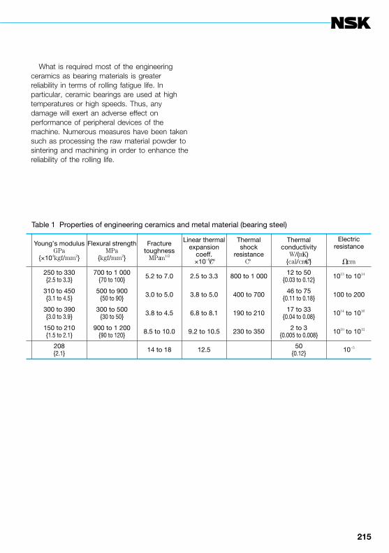
214 215

What is required most of the engineering ceramics as bearing materials is greater reliability in terms of rolling fatigue life. In particular, ceramic bearings are used at high temperatures or high speeds. Thus, any damage will exert an adverse effect on performance of peripheral devices of the machine. Numerous measures have been taken such as processing the raw material powder to sintering and machining in order to enhance the reliability of the rolling life.

Table 1 Properties of engineering ceramics and metal material (bearing steel)

Young,s modulusGPa

{×104kgf/mm2}

Flexural strengthMPa

{kgf/mm2}

Fracturetoughness

MPa≦m1/2

Linear thermalexpansion

coeff.×10−6/°C

Thermalshock

resistance°C

Thermalconductivity

W/(m≦K){cal/cm≦s°C}

Electricresistance

Ω≦cm

250 to 330{2.5 to 3.3}

700 to 1 000{70 to 100} 5.2 to 7.0 2.5 to 3.3 800 to 1 000 12 to 50

{0.03 to 0.12} 1013 to 1014

310 to 450{3.1 to 4.5}

500 to 900{50 to 90} 3.0 to 5.0 3.8 to 5.0 400 to 700 46 to 75

{0.11 to 0.18} 100 to 200

300 to 390{3.0 to 3.9}

300 to 500{30 to 50} 3.8 to 4.5 6.8 to 8.1 190 to 210 17 to 33

{0.04 to 0.08} 1014 to 1016

150 to 210{1.5 to 2.1}

900 to 1 200{90 to 120} 8.5 to 10.0 9.2 to 10.5 230 to 350 2 to 3

{0.005 to 0.008} 1010 to 1012

208{2.1} ≦ 14 to 18 12.5 ≦ 50

{0.12} 10−5

216

Bearing materials

Fig. 1 shows a Weibull plot of the results of a test with radial ball bearings using ceramic balls of silicon nitride of six kinds of HIP (sintered under atmospheric pressure) differing in raw material, structure, and components. The test was conducted, with 3/8” diameter ceramic balls incorporated into inner and outer rings of bearing steel, under conditions of Table 2.

X and Y in Fig. 1 are bearings with NSK-made ceramic balls developed under strict control of the material manufacturing process. A theoretical calculation life (L10) of bearing with steel balls under the same test conditions is 263 hours. It can, therefore, be stated that NSK-made ceramic balls have a life of more than eight times as long as L10 of bearings with steel balls. Other ceramic balls develop flaking while suffering wider variance within a shorter period of time.

The flaking pattern shows a unique fatigue appearance (Photo 1), mostly indicating a type of flaking which is generated by foreign metallic material, segregation of the sintering auxiliary agent, or the occurrence of pores.

The commonly highlighted strength characteristics of engineering ceramics are flexural strength, hardness, and KIC (fracture toughness). Apart from these characteristics, the material needs to be free from defects such as pores or segregation of the auxiliary agent. This can be accomplished through cleaning of the material base and optimum sintering.

Accordingly, due and careful consideration of the material maker is necessary during processing stages from raw material powder to sintering in order to transform ceramics into a an extremely reliable engineering bearing material.

Table 2 Test conditions

Test bearing

Support bearing

Radial load

Max. contact surfacepressure

Speed

Lubrication

6206 with 8 ceramic balls and nylon cage

6304

3 800 N {390 kgf}

2 800 MPa {290 kgf/mm2}

3 000 min−1

FBK oil RO-68

216 217

　　　Fig. 1　Weibull plot of life test results

Photo 1　Appearance of flaking

1　mm

218

Bearing materials

10.7 Physical properties of representative polymers used as bearing material

Because of lightweight, easy formability, and high corrosion resistance, polymer materials are used widely as a material for cages. Polymers may be used independently, but they are usually combined with functional fillers to form a composite material. Composites can be customized to have specific properties. In this way composites can be designed to be bearing materials. For example, fillers can be used to improve such properties as low friction, low wear, non-stick slip characteristic, high limit PV value, non-scrubbing of counterpart material, mechanical properties, and heat resistance, etc.

Table 1 shows characteristics of representative polymer materials used for bearings.

Notes ( 1 )≦GPa≦104 kgf/cm2＝102 kgf/mm2

( 2 )≦If there is a slash mark “/” in the thermal ( 3 )≦Reference value

PlasticsElastic

modulus(GPa) (1)

PolyethyleneHDPEUHMWPE

0.1150.5

PolyamideNylon 6Nylon 66

2.53.0

Nylon 11 1.25

Polytetra fluoroethylenePTFE 0.40

Poly buthylene terephthalatePBT 2.7

PolyacetalPOM

Homo-polymerCo-polymer

3.22.9

Polyether sulfonPES 2.46

PolysulfonPSf 2.5

Polyallylate(Aromatic polyester)

1.33.0

Polyphenylene sulfidePPS (GF 40%) 4.2

Polyether ether ketonPEEK 1.7

Poly-meta-phenyleneisophthalic amide

10(fiber)7.7

(mold)

Polypromellitic imide(Aromatic polyimide) PI

3(film)

2.5 to 3.2(mold)

Polyamide imidePAI 4.7

Polyether imide(Aromatic polyimide) PI 3.6

Polyamino bis-maleimide ≦

218 219

deformation temperature column, then the value to the left of the “/” applies to 451 kPa, If there, the value relates to 1.82 MPa.

Table 1 Characteristics of representative polymers

Strength

GPa (1)

Density

g/cm3

Specificelastic

modulus×104mm

Specificstrength×104mm

Meltingpoint

°C

Glasstransition

temp°C

Thermaldeformationtemperature

°C (2)

Continuousoperating

temperature°C

Remarks

High creep andtoughness,softeningHigh waterabsorption andtoughness

Low waterabsorption

High creep, sintering,lowfriction andadhesion, inert.Stable at 290°C

High ha rdness andtoughness, lowwater absorptionUsable up to200°CChemically stable

Inert, highhardness, Used asfiller for PTFEStable up to 320°CHot cured at360°C

F i re re ta rdant , heatresistance fiber

No change in inertgas up to 350°C

Usable up to300°C for bearing.S i n t e r i n g , n o fusion(molded products)Usable up to290°C as adhesiveor enamelImprovedpolyimide ofmelting formingImprovedpolyimide ofmelting forming

0.030.025

0.960.94

12.653.2

3.32.7

132136

−20−20

75/5075/50

≦≦

0.070.08

1.131.14

221.2263.2

6.27.0

215264

5060

150/57180/60

80 to 12080 to 120

0.04 1.04 120.2 3.8 180 ≦ 150/55Lower than

nylon 6or 66

0.028 2.16 18.5 1.3 327 115 120/≦ 260

0.06 1.31 206.1 4.6 225 30 230/215 155

0.070.06

1.421.41

225.3205.7

4.94.3

175165

−13≦

170/120155/110

≦104

0.086 1.37 179.6 6.3 ≦ 225 210/203 180

0.07 1.24 201.6 5.6 ≦ 190 181/175 150

0.070.075

1.351.40

96.3214.3

5.25.4

350350

≦≦

293293

300260 to 300

0.14 1.64 256.1 8.5 275 94 >260 220

0.093 1.30 130.8 7.2 335 144 152 240

0.70.18

1.381.33

724.6579

50.713.5

375415

(decomposition)

>230>230

280280

220220

0.17 1.43 203 7.0 Heat de-composition

417decomposition 360/250 300 (3)

0.1 1.43 203 7.0 Heat de-composition

417decomposition 360/250 260

0.2 1.41 333.3 14.2 ≦ 280 260 210

0.107 1.27 240.9 ≦ ≦ 215 210/200 170

0.35 1.6 ≦ 21.9 ≦ ≦ 330 (3) 260

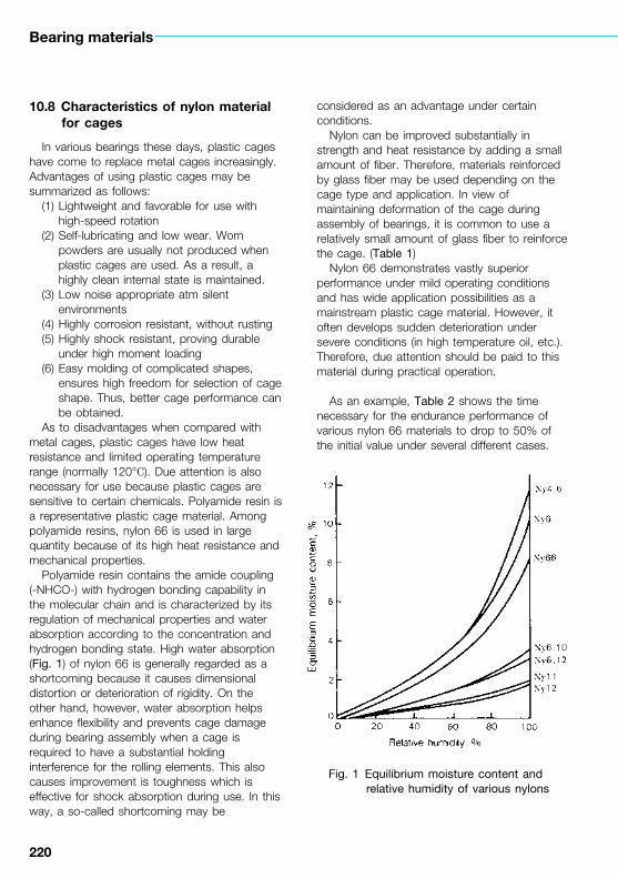
220

Bearing materials

10.8 Characteristics of nylon material for cages

In various bearings these days, plastic cages have come to replace metal cages increasingly. Advantages of using plastic cages may be summarized as follows:

(1) Lightweight and favorable for use with high-speed rotation

(2) Self-lubricating and low wear. Worn powders are usually not produced when plastic cages are used. As a result, a highly clean internal state is maintained.

(3) Low noise appropriate atm silent environments

(4) Highly corrosion resistant, without rusting(5) Highly shock resistant, proving durable

under high moment loading(6) Easy molding of complicated shapes,

ensures high freedom for selection of cage shape. Thus, better cage performance can be obtained.

As to disadvantages when compared with metal cages, plastic cages have low heat resistance and limited operating temperature range (normally 120°C). Due attention is also necessary for use because plastic cages are sensitive to certain chemicals. Polyamide resin is a representative plastic cage material. Among polyamide resins, nylon 66 is used in large quantity because of its high heat resistance and mechanical properties.

Polyamide resin contains the amide coupling (-NHCO-) with hydrogen bonding capability in the molecular chain and is characterized by its regulation of mechanical properties and water absorption according to the concentration and hydrogen bonding state. High water absorption (Fig. 1) of nylon 66 is generally regarded as a shortcoming because it causes dimensional distortion or deterioration of rigidity. On the other hand, however, water absorption helps enhance flexibility and prevents cage damage during bearing assembly when a cage is required to have a substantial holding interference for the rolling elements. This also causes improvement is toughness which is effective for shock absorption during use. In this way, a so-called shortcoming may be

considered as an advantage under certain conditions.

Nylon can be improved substantially in strength and heat resistance by adding a small amount of fiber. Therefore, materials reinforced by glass fiber may be used depending on the cage type and application. In view of maintaining deformation of the cage during assembly of bearings, it is common to use a relatively small amount of glass fiber to reinforce the cage. (Table 1)

Nylon 66 demonstrates vastly superior performance under mild operating conditions and has wide application possibilities as a mainstream plastic cage material. However, it often develops sudden deterioration under severe conditions (in high temperature oil, etc.). Therefore, due attention should be paid to this material during practical operation.

As an example, Table 2 shows the time necessary for the endurance performance of various nylon 66 materials to drop to 50% of the initial value under several different cases.

Fig. 1　Equilibrium moisture content and relative humidity of various nylons

220 221

Material deterioration in oil varies depending on the kind of oil. Deterioration is excessive if the oil contains an extreme-pressure agent. It is known that sulfurous extreme-pressure agents accelerate deterioration more than phosphorous extreme-pressure agents and such deterioration occurs more rapidly with rising temperatures.

On the other hand, material deteriorates less in grease or air than in oil. Besides, materials reinforced with glass fiber can suppress deterioration of the strength through material deterioration by means of the reinforcement effect of glass fibers, thereby, helping to extend the durability period.

Class content: A<B<C<D

Table 1 Examples of applications with fiber reinforced nylon cages

Rol

ler

bea

ring

Bal

l bea

ring

Bearing type Main aplication Cage material

Miniature ball bearings

Deep groove ball bearings

Angular contact ball bearings

VCR, IC cooling fans

Alternators, fan motors for airconditioners

Magnetic clutches, automotivewheels

Nylon 66(Glass fiber content: 0 to 10%)

Needle roller bearings

Tapered roller bearings

ET-type cylindrical roller bearings

H-type spherical roller bearings

Automotive transmissions

Automotive wheels

General

General

Nylon 66(Glass fiber content: 10 to 25%)

Table 2 Environmental resistance of nylon 66 resin

▲▲

▲▲

▲▲

▲▲

▲▲

▲▲

▲▲

▲▲

▲▲

▲▲

▲▲

Hours for the physical property value to drop to 50%, h 500 1000 1500 2000 Remarks

C o n t a i n s anextreme pressureadditiveC o n t a i n s anextremepressureadditive

C o n t a i n s anextremepressureadditive

Environment Temper-ature, °C

Glasscontent

Oil

Gear oil

Syn

thet

ic

lub

ricat

ing

oil

Hydraulic oil

ATF oil

Engine oil

Grease

Air

120 0D

1400AD

100 A

120 A

1300AC

1500BD

80 0D

120 0D

150 0D

120 0D

1400AD

120 0D

80 0D

120 0D

130 AD

1600AC

180 0B

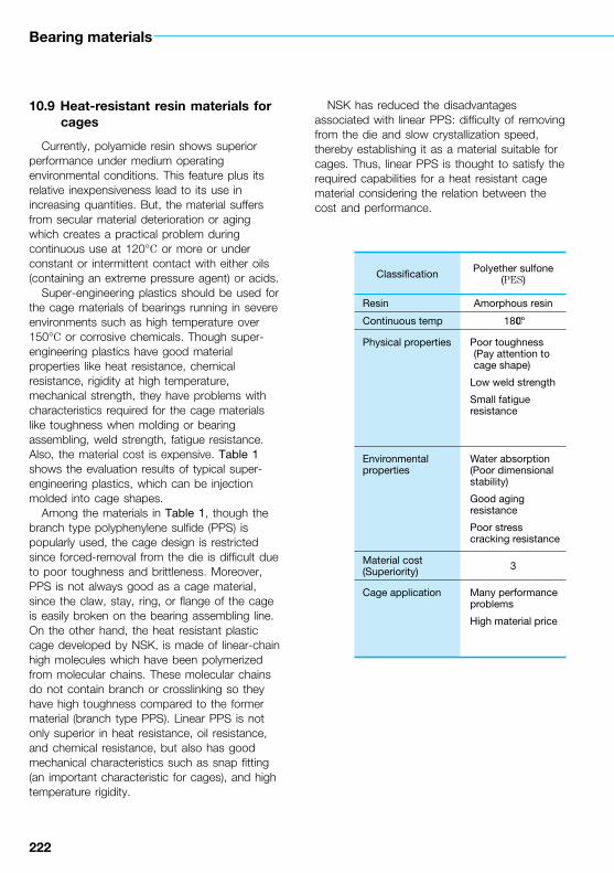
222

Bearing materials

10.9 Heat-resistant resin materials for cages

Currently, polyamide resin shows superior performance under medium operating environmental conditions. This feature plus its relative inexpensiveness lead to its use in increasing quantities. But, the material suffers from secular material deterioration or aging which creates a practical problem during continuous use at 120°C or more or under constant or intermittent contact with either oils (containing an extreme pressure agent) or acids.

Super-engineering plastics should be used for the cage materials of bearings running in severe environments such as high temperature over 150°C or corrosive chemicals. Though super-engineering plastics have good material properties like heat resistance, chemical resistance, rigidity at high temperature, mechanical strength, they have problems with characteristics required for the cage materials like toughness when molding or bearing assembling, weld strength, fatigue resistance. Also, the material cost is expensive. Table 1 shows the evaluation results of typical super-engineering plastics, which can be injection molded into cage shapes.

Among the materials in Table 1, though the branch type polyphenylene sulfide (PPS) is popularly used, the cage design is restricted since forced-removal from the die is difficult due to poor toughness and brittleness. Moreover, PPS is not always good as a cage material, since the claw, stay, ring, or flange of the cage is easily broken on the bearing assembling line. On the other hand, the heat resistant plastic cage developed by NSK, is made of linear-chain high molecules which have been polymerized from molecular chains. These molecular chains do not contain branch or crosslinking so they have high toughness compared to the former material (branch type PPS). Linear PPS is not only superior in heat resistance, oil resistance, and chemical resistance, but also has good mechanical characteristics such as snap fitting (an important characteristic for cages), and high temperature rigidity.

NSK has reduced the disadvantages associated with linear PPS: difficulty of removing from the die and slow crystallization speed, thereby establishing it as a material suitable for cages. Thus, linear PPS is thought to satisfy the required capabilities for a heat resistant cage material considering the relation between the cost and performance.

Classification Polyether sulfone(PES)

Resin Amorphous resin

Continuous temp 180°C

Physical properties ≦Poor toughness(Pay attention tocage shape)

≦Low weld strength

≦Small fatigue≦resistance

Environmentalproperties

≦Water absorption≦(Poor dimensional≦stability)

≦Good aging≦resistance

≦Poor stress≦cracking resistance

Material cost(Superiority) 3

Cage application ≦Many performance≦problems

≦High material price

222 223

Table 1 Properties of typical super-engineering plastic materials for cages

Polyether imide(PEI)

Polyamide imide(PAI)

Polyether etherketon(PEEK)

Branch typepolyphenylenesulfide (PPS)

Linear typepolyphenylenesulfide (L-PPS)

Amorphous resin Amorphous resin Crystalline resin Crystalline resin Crystalline resin

170°C 210°C 240°C 220°C 220°C

≦Poor toughness

≦Small weld strength

≦Small fatigue≦resistance

≦Very brittle (No≦forced-removal≦molding)

≦Special heat≦treatment before≦use

≦High rigidity, after≦heat treatment

≦Excellent≦toughness, wear≦and fatigue≦resistance

≦Small weld strength

≦Excellent≦mechanical≦properties

≦Slightly low≦toughness

≦Excellent≦mechanical≦properties

≦Good toughness

≦Good dimensional≦stability (No water≦absorption)

≦Good aging≦resistance

≦Poor stress≦cracking resistance

≦Good environment≦resistance



≦Good environment≦resistance (Not≦affected by most≦chemicals. Doesn

,t

≦deteriorate in high≦temperature oil with≦extreme pressure≦additives).

2 5 4 1 1

≦Many performance≦problems

≦High material cost

≦Good performance

≦High material and≦molding cost (For≦special applications)

≦Excellent≦performance

≦High material cost≦(For special≦applications)

≦Problems with≦toughness

≦Cost is high≦compared to its≦performance

≦Reasonable cost for≦its performance≦(For general≦applications)

224

Bearing materials

10.10 Features and operating temperature range of ball bearing seal material

The sealed ball bearing is a ball bearing with seals as shown in Figs. 1 and 2. There are two seal types: non-contact seal type and contact seal type. For rubber seal material, nitrile rubber is used for general purpose and poly-acrylic rubber, silicon rubber, and fluoric rubber are used depending on temperature conditions.

These rubbers have their own unique nature and appropriate rubber must be selected by considering the particular application environment and running conditions.

Table 1 shows principal features of each rubber material and the operating temperature range of the bearing seal. The operating temperature range of Table 1 is a guideline for continuous operation. Thermal aging of rubber is related to the temperature and time. Rubber may be used in a much wider range of operating temperatures depending on the operating time and frequency.

In the non-contact seal, heat generation due to friction on the lip can be ignored. And thermal factors, which cause aging of the rubber, are physical changes due to atmospheric and bearing temperatures. Accordingly, increased hardness or loss of elasticity due to thermal aging exerts only a negligible effect on the seal performance. A rubber non-contact seal can thus be used in an expanded range of operating temperatures greater than that for a contact seal.

But there are some disadvantages. The contact seal has a problem with wear occurring at the seal lip due to friction, thermal plastic deformation, and hardening. When friction or plastic deformation occurs, the contact pressure between the lip and slide surface decreases, resulting in a clearance. This clearance is minimum and does not cause excessive degradation of sealing performance (for instance, it does not allow dust entry or grease leakage). In most cases, this minor plastic deformation or slightly increased hardness presents no practical problems.

However, in external environments with dust and water in large quantity, the bearing seal is used as an auxiliary seal and a principal seal should be provided separately. As so far described, the operating temperature range of rubber material is only a guideline for selection. Since heat resistant rubber is expensive, it is important to understand the temperature conditions so that an economical selection can be made. Due attention should also be paid not only to heat resistance, but also to the distinctive features of each rubber.

Fig. 1 Fig. 2

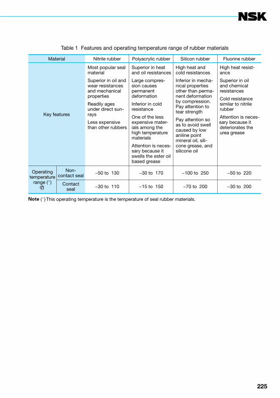
224 225

Table 1 Features and operating temperature range of rubber materials

Material Nitrile rubber Polyacrylic rubber Silicon rubber Fluorine rubber

Key features

≦Most popular seal≦material

≦Superior in oil and≦wear resistances≦and mechanical≦properties

≦Readily ages≦under direct sun-≦rays

≦Less expensive≦than other rubbers

≦Superior in heat≦and oil resistances

≦Large compres-≦sion causes≦permanent≦deformation

≦Inferior in cold≦resistance

≦One of the less≦expensive mater-≦ials among the≦high temperature≦materials

≦Attention is neces-≦sary because it ≦swells the ester oil≦based grease

≦High heat and≦cold resistances

≦Inferior in mecha-≦nical properties≦other than perma-≦nent deformation≦by compression.≦Pay attention to≦tear strength

≦Pay attention so≦as to avoid swell≦caused by low≦aniline point≦mineral oil, sili-≦cone grease, and≦silicone oil

≦High heat resist-≦ance

≦Superior in oil≦and chemical≦resistances

≦Cold resistance≦similar to nitrile≦rubber

≦Attention is neces-≦

sary because it ≦deteriorates the ≦urea grease

Operatingtemperature

range ( 1 )(°C)

Non-contact seal −50 to ≦130 −30 to ≦170 −100 to ≦250 −50 to ≦220

Contactseal −30 to ≦110 −15 to ≦150 −70 to ≦200 −30 to ≦200

Note ( 1 )≦This operating temperature is the temperature of seal rubber materials.

226

11. Load calculation of gears

11.1 Calculation of loads on spur, helical, and double-helical gears

There is an extremely close relationship among the two mechanical elements, gears and rolling bearings. Gear units, which are widely used in machines, are almost always used with bearings. Rating life calculation and selection of bearings to be used in gear units are based on the load at the gear meshing point.

The load at the gear meshing point is calculated as follows:

Spur gear:

P1=P2= =

............................................. (N)

= = ....... {kgf}

S1=S2=P1tana

The magnitudes of the forces P2 and S2 applied to the driven gear are the same as P1 and S1 respectively, but the direction is opposite.

Helical gear:

P1=P2= =

............................................. (N)

= = ....... {kgf}

S1=S2=

T1=T2=P1tanb

The magnitudes of the forces P2, S2, and T2 applied to the driven gear are the same as P1, S1, and T1 respectively, but the direction is opposite.

Double-helical gear:

P1=P2= =

............................................. (N)

= = ....... {kgf}

S1=S2=

where, P: Tangential force (N), {kgf} S: Separating force (N), {kgf} T: Thrust (N), {kgf} H: Transmitted power (kW) n: Speed (min–1) dp: Pitch diameter (mm) a: Gear pressure angle an: Gear normal pressure angle b: Twist angle

Subscript 1: Driving gearSubscript 2: Driving gear

In the case of double-helical gears, thrust of the helical gears offsets each other and thus only tangential and separating forces act. For the directions of tangential, separating, and thrust forces, please refer to Figs. 1 and 2.

P1tanan

cosb

9 550 000H

n1 ( dp1 )2

9 550 000H

n2 ( dp2 )2

974 000H

n1 ( dp1 )2

974 000H

n2 ( dp2 )2

9 550 000H

n1 ( dp1 )2

9 550 000H

n2 ( dp2 )2

974 000H

n1 ( dp1 )2

974 000H

n2 ( dp2 )2

P1tanan

cosb

9 550 000H

n1 ( dp1 )2

9 550 000H

n2 ( dp2 )2

974 000H

n1 ( dp1 )2

974 000H

n2 ( dp2 )2

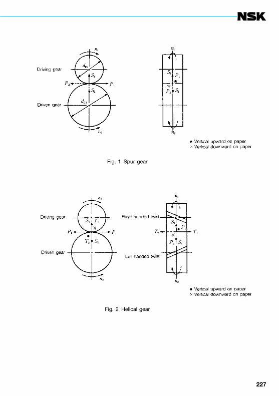
226 227

Fig. 1　Spur gear

Fig. 2　Helical gear

228

Load calculation of gears

The thrust direction of the helical gear varies depending on the gear running direction, gear twist direction, and whether the gear is driving or driven.The directions are as follows:

The force on the bearing is determined as follows:

Tangential force:

P1=P2= =

............................................. (N)

= = ....... {kgf}

Separating force: S1=S2=P1

Thrust: T1=T2=P1· tanb

The same method can be applied to bearings C and D.

tanan

cosb

9 550 000H

n1 ( dp1 )2

9 550 000H

n2 ( dp2 )2

974 000H

n1 ( dp1 )2

974 000H

n2 ( dp2 )2

Load direction is shown referring to left side of Fig. 3.

Table 1

Rad

ial l

oad

Loadclassification Bearing A Bearing B

FromP1

　　　bPA＝───P1　　⊗　　 a＋b

　　　aPB＝───P1　　⊗　　 a＋b

FromS1

　　　bSA＝───S1　　扌　　 a＋b

　　　aSB＝───S1　　扌　　 a＋b

FromT1

　　dp1/2UA＝───T1　　扌　　 a＋b

　　dp1/2UB＝───T1　　➡　　 a＋b

Combinedradial load FrA＝　 PA

2＋（SA＋UA）2 FrB＝　PB2＋（SB−UB）2

Axial load 　　　　　　　　Fa＝T1　　➡

Fig. 3

228 229

Fig. 4　Thrust direction

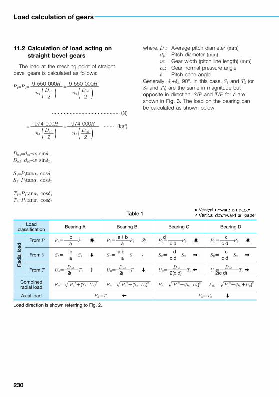
230


11.2 Calculation of load acting on straight bevel gears

The load at the meshing point of straight bevel gears is calculated as follows:

P1=P2= =

............................................. (N)

= = ....... {kgf}

Dm1=dp1–w sind1

Dm2=dp2–w sind2

S1=P1tanan cosd1

S2=P2tanan cosd2

T1=P1tanan cosd1

T2=P2tanan cosd2

where, Dm: Average pitch diameter (mm) dp: Pitch diameter (mm) w: Gear width (pitch line length) (mm) an: Gear normal pressure angle d: Pitch cone angleGenerally, d1+d2=90°. In this case, S1 and T2 (or S2 and T1) are the same in magnitude but opposite in direction. S/P and T/P for d are shown in Fig. 3. The load on the bearing can be calculated as shown below.

9 550 000H

n1 ( Dm1 )2

9 550 000H

n2 ( Dm2 )2

974 000H

n1 ( Dm1 )2

974 000H

n2 ( Dm2 )2

Load direction is shown referring to Fig. 2.

Table 1

Rad

ial l

oad

Loadclassification Bearing A Bearing B Bearing C Bearing D

From P　　　bPA＝───P1　　 ◉　　　a

　　 a＋bPB＝───P1　　 ⊗　　　a

　　　dPC＝───P2　　 ◉　　 c　d

　　　cPD＝───P2　　 ◉　　 c　d

From S　　　bSA＝───S1 　　 ➡　　　a

　　 a　bSB＝───S1　　扌　　　a

　　　dSC＝───S2　　 ➡　　 c　d

　　　cSD＝───S2　　 ➡　　 c　d

From T　　　Dm1UA＝───T1 　扌　　　2　a

　　　Dm1UB＝───T1 　 ➡　　　2　a　　　　Dm2UC＝────T2 ➡　　2(c　d)

　　　　Dm2UD＝────T2 ➡　　 2(c　d)

Combinedradial load FrA＝　PA

2＋(SA−UA)2 FrB＝　PB2＋(SB−UB)2 FrC＝　PC

2＋(SC−UC)2 FrD＝　PD2＋(SD＋UD)2

Axial load Fa＝T1　　　➡ Fa＝T2　　　➡

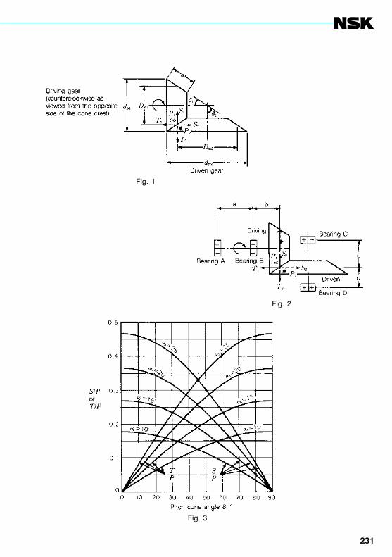
230 231

Fig. 1

Fig. 2

Fig. 3

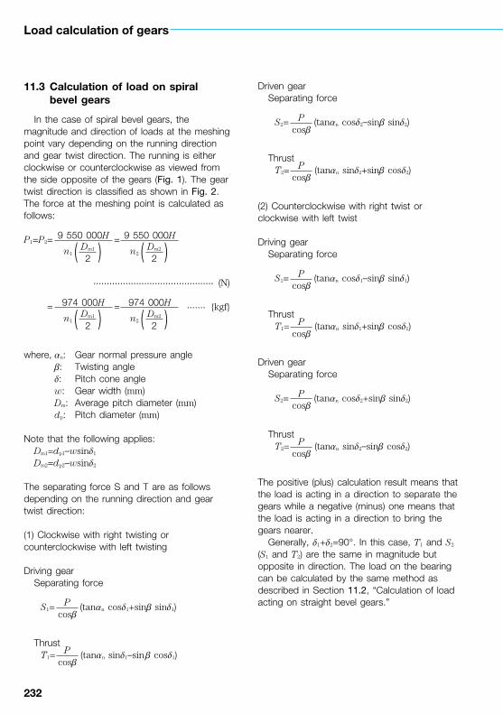
232


11.3 Calculation of load on spiral bevel gears

In the case of spiral bevel gears, the magnitude and direction of loads at the meshing point vary depending on the running direction and gear twist direction. The running is either clockwise or counterclockwise as viewed from the side opposite of the gears (Fig. 1). The gear twist direction is classified as shown in Fig. 2. The force at the meshing point is calculated as follows:

P1=P2= =

............................................. (N)

= = ....... {kgf}

where, an: Gear normal pressure angle b: Twisting angle d: Pitch cone angle w: Gear width (mm) Dm: Average pitch diameter (mm) dp: Pitch diameter (mm)

Note that the following applies:Dm1=dp1–wsind1

Dm2=dp2–wsind2

The separating force S and T are as follows depending on the running direction and gear twist direction:

(1) Clockwise with right twisting or counterclockwise with left twisting

Driving gearSeparating force

S1= (tanan cosd1+sinb sind1)

ThrustT1= (tanan sind1–sinb cosd1)

Driven gearSeparating force

S2= (tanan cosd2–sinb sind2)

ThrustT2= (tanan sind2+sinb cosd2)

(2) Counterclockwise with right twist or clockwise with left twist


S1= (tanan cosd1–sinb sind1)

ThrustT1= (tanan sind1+sinb cosd1)


S2= (tanan cosd2+sinb sind2)

ThrustT2= (tanan sind2–sinb cosd2)

The positive (plus) calculation result means that the load is acting in a direction to separate the gears while a negative (minus) one means that the load is acting in a direction to bring the gears nearer.

Generally, d1+d2=90°. In this case, T1 and S2 (S1 and T2) are the same in magnitude but opposite in direction. The load on the bearing can be calculated by the same method as described in Section 11.2, “Calculation of load acting on straight bevel gears.”

9 550 000H

n1 ( Dm1 )2

9 550 000H

n2 ( Dm2 )2

974 000H

n1 ( Dm1 )2

974 000H

n2 ( Dm2 )2

Pcosb

Pcosb

Pcosb

Pcosb

Pcosb

Pcosb

Pcosb

Pcosb

232 233

Fig. 1

Fig. 2

Fig. 3

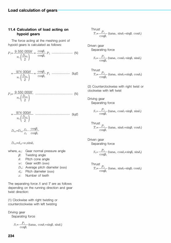
234


11.4 Calculation of load acting on hypoid gears

The force acting at the meshing point of hypoid gears is calculated as follows:

P1= = P2 ....................... (N)

= = P2 .................... {kgf}

P2= ......................................... (N)

= ...................................... {kgf}

Dm1=Dm2 ·

Dm2=dp2–w2sind2

where, an: Gear normal pressure angle b: Twisting angle d: Pitch cone angle w: Gear width (mm) Dm: Average pitch diameter (mm) dp: Pitch diameter (mm) z: Number of teeth

The separating force S and T are as follows depending on the running direction and gear twist direction:

(1) Clockwise with right twisting or counterclockwise with left twisting


S1= (tanan cosd1+sinb1 sind1)

ThrustT1= (tanan sind1–sinb1 cosd1)


S2= (tanan cosd2–sinb2 sind2)

ThrustT2= (tanan sind2+sinb2 cosd2)

(2) Counterclockwise with right twist or clockwise with left twist


S1= (tanan cosd1–sinb1 sind1)

ThrustT1= (tanan sind1+sinb1 cosd1)


S2= (tanan cosd2+sinb2 sind2)

ThrustT2= (tanan sind2–sinb2 cosd2)

9 550 000H

n1 ( Dm1 )2

974 000H

n1 ( Dm1 )2

cosb1

cosb2

cosb1

cosb2

9 550 000H

n2 ( Dm2 )2

974 000H

n2 ( Dm2 )2

z1

z2

cosb1

cosb2

P1

cosb1

P1

cosb1

P2

cosb2

P2

cosb2

P1

cosb1

P2

cosb2

P2

cosb2

P1

cosb1

234 235

The positive (plus) calculation result means that the load is acting in a direction to separate the gears while a negative (minus) one means that the load is acting in a direction to bring the gears nearer.

For the running direction and gear twist direction, refer to Section 11.3, “Calculation of load on spiral bevel gears.” The load on the bearing can be calculated by the same method as described in Section 11.2, “Calculation of load acting on straight bevel gears.”

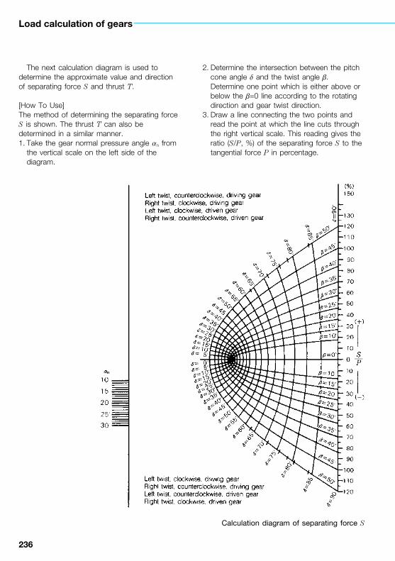
236


The next calculation diagram is used to determine the approximate value and direction of separating force S and thrust T.

[How To Use]The method of determining the separating force S is shown. The thrust T can also be determined in a similar manner.1. Take the gear normal pressure angle an from

the vertical scale on the left side of the diagram.

2. Determine the intersection between the pitch cone angle d and the twist angle b. Determine one point which is either above or below the b=0 line according to the rotating direction and gear twist direction.

3. Draw a line connecting the two points and read the point at which the line cuts through the right vertical scale. This reading gives the ratio (S/P, %) of the separating force S to the tangential force P in percentage.

Calculation diagram of separating force S Calculation diagram of thrust T

236 237

Calculation diagram of separating force S Calculation diagram of thrust T

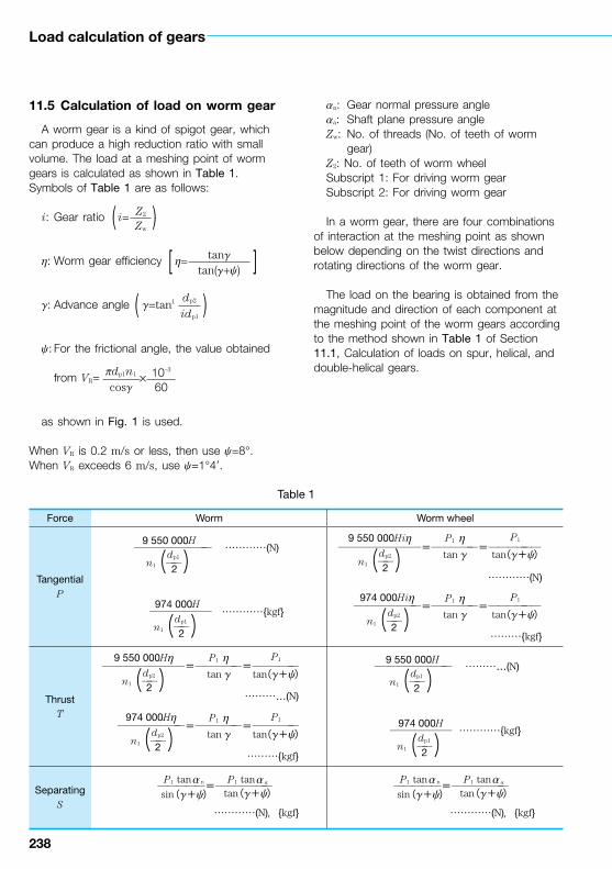
238


11.5 Calculation of load on worm gear

A worm gear is a kind of spigot gear, which can produce a high reduction ratio with small volume. The load at a meshing point of worm gears is calculated as shown in Table 1. Symbols of Table 1 are as follows:

i: Gear ratio i=

h: Worm gear efficiency h=

g: Advance angle g=tan1

y: For the frictional angle, the value obtained

from VR= ´

as shown in Fig. 1 is used.

When VR is 0.2 m/s or less, then use y=8°.When VR exceeds 6 m/s, use y=1°4’.

an: Gear normal pressure angleaa: Shaft plane pressure angleZw: No. of threads (No. of teeth of worm

gear)Z2: No. of teeth of worm wheelSubscript 1: For driving worm gearSubscript 2: For driving worm gear

In a worm gear, there are four combinations of interaction at the meshing point as shown below depending on the twist directions and rotating directions of the worm gear.

The load on the bearing is obtained from the magnitude and direction of each component at the meshing point of the worm gears according to the method shown in Table 1 of Section 11.1, Calculation of loads on spur, helical, and double-helical gears.

Z2

Zw( )

tangtan(g+y)[ ]

dp2

idp1( )

10–3

60pdp1n1

cosg

Table 1

Force Worm Worm wheel

TangentialP

ThrustT

SeparatingS

──────── …………(N)

　　────── …………{kgf}

9 550 000H

974 000H

　　dp1n1　──　　　2( )

　　dp1n1　──　　　2( )

────────＝─────＝─────

…………(N)

　 ───────＝─────＝─────

………{kgf}

　　dp2n1　──　　　2( )

9 550 000Hh

974 000Hh

P1 h P1

　　dp2n1　──　　　2( )

tan g tan（g＋y）

P1 h P1


─────＝──────

　　　　　 …………(N)，{kgf}

P1 tana n

tan（g＋y）sin（g＋y）P1 tana a

────────＝─────＝──────

…………(N)

　 ───────＝─────＝──────

………{kgf}

　　dp2n1　──　　　2( )

9 550 000Hih

974 000Hih

P1 h P1

　　dp2n1　──　　　2( )


P1 h P1


──────── …………(N)

　　────── …………{kgf}

9 550 000H

974 000H

　　dp1n1　──　　　2( )

　　dp1n1　──　　　2( )─────＝──────

　　　　　 …………(N)，{kgf}

P1 tana n

tan（g＋y）sin（g＋y）P1 tana a

238 239

Fig. 1

Fig. 2.1　Right twist worm gear

Fig. 2.2　Right twist worm gear (Worm rotation is opposite that of Fig. 2.1)

Fig. 2.3　Left twist worm gear

Fig. 2.4　Left twist worm gear (Worm rotation is opposite that of Fig. 2.3)

240

12. General miscellaneous information

12.1 JIS concerning rolling bearings

Rolling bearings are critical mechanical elements which are used in a wide variety of machines. They are standardized internationally by ISO (International Organization for Stan dardization). Standards concerning rolling bearings can also be found in DIN (Germany), ANSI (USA), and BS (England). In Japan, the conventional JIS standards related to rolling bearings are arranged systematically and revised in accordance to the JIS standards enacted in 1965. Since then, these have been individually revised in reference to the ISO standards or compliance with the actual state of production and sales.

Most of the standard bearings manufactured in Japan are based on the JIS standards. BAS (Japan Bearing Association Standards), on the other hand, acts as a supplement to JIS. Table 1 lists JIS standards related to bearings.

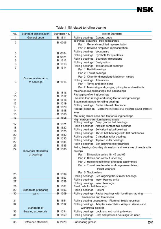
240 241

No. Standard classification Standard No. Title of Standard 1 General code B 1511 Rolling bearings ― General code

2

3 4 5 6 7

8

910111213141516

Common standardsof bearings

B 0005

B 0104B 0124B 1512B 1513B 1514

B 1515

B 1516B 1517B 1518B 1519B 1520B 1548B 1566G 4805

Technical drawings ― Rolling bearings――――― Part 1: General simplified representation――――― Part 2: Detailed simplified representationRolling bearings ― VocabularyRolling bearings ― Symbols for quantitiesRolling bearings ― Boundary dimensionsRolling bearings ― DesignationRolling bearings ― Tolerances of bearings――――― Part 1: Radial bearings――――― Part 2: Thrust bearings――――― Part 3: Chamfer dimensions-Maximum valuesRolling bearings ― Tolerances――――― Part 1: Terms and definitions――――― Part 2: Measuring and gauging principles and methodsMaking on rolling bearings and packagingsPackaging of rolling bearingsDynamic load ratings and rating life for rolling bearingsStatic load ratings for rolling bearingsRolling bearings ― Radial internal clearanceRolling bearings ― Measuring methods of A-weighted sound pressure levelsMounting dimensions and fits for rolling bearingsHigh carbon chromium bearing steels

1718192021222324

252627

Individual standardsof bearings

B 1521B 1522B 1523B 1532B 1533B 1534B 1535B 1536

B 1539B 1557B 1558

Rolling bearings ― Deep groove ball bearingsRolling bearings ― Angular contact ball bearingsRolling bearings ― Self-aligning ball bearingsRolling bearings ― Thrust ball bearings with flat back facesRolling bearings ― Cylindrical roller bearingsRolling bearings ― Tapered roller bearingsRolling bearings ― Self-aligning roller bearingsRolling bearings-Boundary dimensions and tolerances of needle roller bearings――――― Part 1: Dimension series 48, 49 and 69――――― Part 2: Drawn cup without inner ring――――― Part 3: Radial needle roller and cage assemblies――――― Part 4: Thrust needle roller and cage assemblies, thrust washers――――― Part 5: Track rollersRolling bearings ― Self-aligning thrust roller bearingsRolling bearings ― Insert bearing unitsRolling bearings ― Insert bearings

282930

Standards of bearingparts

B 1501B 1506B 1509

Steel balls for ball bearingsRolling bearings ― RollersRolling bearings ― Radial bearings with locating snap ring―――――――――― Dimensions and tolerances

3132

3334

Standards ofbearing accessorie

B 1551B 1552

B 1554B 1559

Rolling bearing accessories ― Plummer block housingsRolling bearings ― Adapter assemblies, Adapter sleeves and――――――― ― Withdrawal sleevesRolling bearings ― Locknuts and locking devicesRolling bearings ― Cast and pressed housings for insert――――――― ― bearings

35 Reference standard K 2220 Lubricating grease

Table 1 JIS related to rolling bearing

242

General miscellaneous information

12.2 Amount of permanent deformation at point where inner and outer rings contact rolling element

When two materials are in contact, a point within the contact zone develops local permanent deformation if it is exposed to a load exceeding the elastic limit of the material. The rolling and raceway surfaces of a bearing, which appear to be perfect to a human eye, are found to be imperfect when observed by microscope even though the surfaces are extremely hard and finished to an extreme accuracy. Therefore, the true contact area is surprisingly small when compared with the apparent contact area, because the surface is actually jagged and rough with asperities or sharp points. These local points develop permanent deformation when exposed to a relatively small load. Such microscopic permanent deformations seldom affect the function of the bearing. Usually, the only major change is that light is reflected differently from the raceway surface (running marks, etc.).

As the load grows further, the amount of permanent deformation increases corresponding to the degree identifiable on the macroscopic scale in the final stage. Fig. 1 shows the manner of this change. While the load is small, the elastic displacement during point contact in a ball bearing is proportional to the pth power of the load Q (p=2/3 for ball bearings and p=0.9

for roller bearings) in compliance with the Hertz theory. The amount of permanent deformation grows as the load increases, resulting in substantial deviation of the elastic displacement from the theoretical value.

For normal bearings, about 1/3 of the gross amount of permanent deformation dq occurs in rolling element and about 2/3 in the bearing ring.

12.2.1 Ball bearingsThe amount of permanent deformation dq can

also be expressed in relation to the load Q. Equation (1) shows the relationship between dq and Q for ball bearings:

dq=1.30´10–7 (rI1+rII1) (rI2+rII2)

...................... (N)

=1.25´10–5 (rI1+rII1) (rI2+rII2)

.................... {kgf}

(mm) ..................................... (1)

where, dq: Gross amount of permanent deformation between the rolling element and bearing ring (mm)

Q: Load of rolling element (N), {kgf} Dw: Diameter of rolling element (mm) rI1, rI2 and rII1, rII2: Take the reciprocal of the main

radius of curvature of the area

where materials I and II make contact (Units: 1/mm).

When the equation is rewritten using the relation between dq and Q, Equation (2) is obtained:

dq=K ·Q2 (N) (mm)

............ (2)=96.2K ·Q2 {kgf}

The value of the constant K is as shown for the bearing series and bore number in Table 1. Ki applies to the contact between the inner ring and rolling element while Ke to that between the outer ring and rolling element.

Q2

Dw

Q2

Dw

Fig. 1

242 243

Table 1 Value of the constant K for deep groove ball bearings

Bearingbore No.

Bearing series 60 Bearing series 62 Bearing series 63

Ki Ke Ki Ke Ki Ke

―――×10−10 ―――×10−10 ―――×10−10 ―――×10−10 ―――×10−10 ―――×10−10

00

01

02

03

04

05

06

07

08

09

10

11

12

13

14

15

16

17

18

19

20

22

24

26

28

30

2.10

2.03

1.94

1.89

0.279

0.270

0.180

0.127

0.417

0.312

0.308

0.187

0.185

0.183

0.119

0.118

0.0814

0.0808

0.0581

0.0576

0.0574

0.0296

0.0293

0.0229

0.0227

0.0181

4.12

1.25

2.21

2.24

0.975

0.997

0.703

0.511

0.311

0.234

0.236

0.140

0.141

0.142

0.0914

0.0920

0.0624

0.0628

0.0446

0.0449

0.0450

0.0225

0.0227

0.0178

0.0179

0.0143

2.01

0.376

0.358

0.236

0.139

0.133

0.0747

0.0460

0.129

0.127

0.104

0.0728

0.0547

0.0469

0.0407

0.0402

0.0309

0.0243

0.0194

0.0158

0.0130

0.00928

0.00783

0.00666

0.00656

0.00647

2.16

1.13

1.16

0.792

0.481

0.494

0.237

0.178

0.0864

0.0875

0.0720

0.0501

0.0377

0.0326

0.0283

0.0286

0.0218

0.0170

0.0136

0.0110

0.00900

0.00639

0.00544

0.00467

0.00472

0.00477

0.220

0.157

0.145

0.107

0.0808

0.0597

0.0379

0.0255

0.0206

0.0436

0.0333

0.0262

0.0208

0.0169

0.0138

0.0117

0.00982

0.00832

0.00710

0.00611

0.00465

0.00326

0.00320

0.00255

0.00209

0.00205

0.808

0.449

0.469

0.353

0.226

0.218

0.119

0.0968

0.0692

0.0270

0.0207

0.0162

0.0218

0.0105

0.00863

0.00733

0.00616

0.00523

0.00447

0.00386

0.00292

0.00203

0.00205

0.00164

0.00134

0.00136

244


As an example, the dq and Q relation may be illustrated as shown in Fig. 2 for the 62 series of deep groove ball bearings.

12.2.2 Roller bearingsIn the case of roller bearings, the permanent

deformation dq and load Q between the rolling element and bearing ring may be related as shown in Equation (3).

dq=2.12´10–11 · · 3

· ( rI+rII1)3/2

...................... (N)

=2.00´10–8 · · 3

· ( rI+rII1)3/2

.................... {kgf}

(mm) ..................................... (3)

1Dw√—

QLwe

( )

1Dw√—

QLwe

( )

Fig. 2　Load and permanent deformation of rolling element

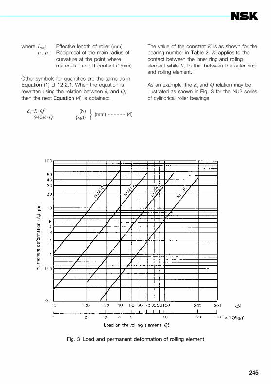
244 245

where, Lwe: Effective length of roller (mm) rI, rII: Reciprocal of the main radius of

curvature at the point where materials I and II contact (1/mm)

Other symbols for quantities are the same as in Equation (1) of 12.2.1. When the equation is rewritten using the relation between dq and Q, then the next Equation (4) is obtained:

dq=K ·Q3 (N) (mm)

............ (4)=943K ·Q2 {kgf}

The value of the constant K is as shown for the bearing number in Table 2. Ki applies to the contact between the inner ring and rolling element while Ke to that between the outer ring and rolling element.

As an example, the dq and Q relation may be illustrated as shown in Fig. 3 for the NU2 series of cylindrical roller bearings.

Fig. 3　Load and permanent deformation of rolling element

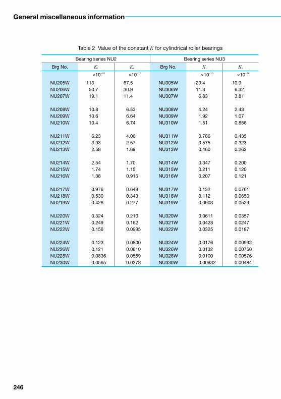
246


Table 2 Value of the constant K for cylindrical roller bearings

Bearing series NU2 Bearing series NU3

Brg No. Ki Ke Brg No. Ki Ke

――――×10−16 ――――×10−16 ――――×10−16 ――――×10−16

NU205WNU206WNU207W

NU208WNU209WNU210W

NU211WNU212WNU213W

NU214WNU215WNU216W

NU217WNU218WNU219W

NU220WNU221WNU222W


11350.719.1

10.810.610.4

6.233.932.58

2.541.741.38

0.9760.5300.426

0.3240.2490.156

0.1230.1210.08360.0565

67.530.911.4

6.536.646.74

4.062.571.69

1.701.150.915

0.6480.3430.277

0.2100.1620.0995

0.08000.08100.05590.0378

NU305WNU306WNU307W

NU308WNU309WNU310W

NU311WNU312WNU313W

NU314WNU315WNU316W

NU317WNU318WNU319W

NU320WNU321WNU322W


20.411.3

6.83

4.241.921.51

0.7860.5750.460

0.3470.2110.207

0.1320.1120.0903

0.06110.04280.0325

0.01760.01320.01000.00832

10.96.323.81

2.431.070.856

0.4350.3230.262

0.2000.1200.121

0.07610.06500.0529

0.03570.02470.0187

0.009920.007500.005760.00484

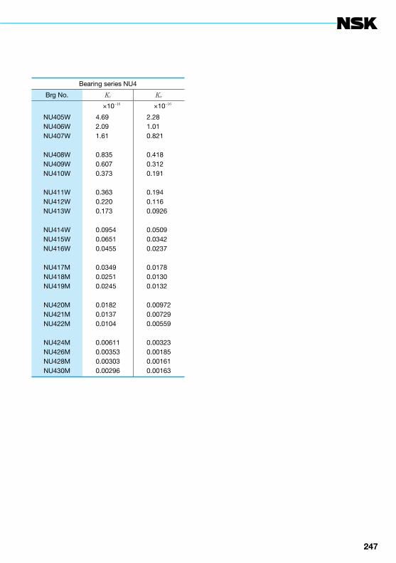
246 247

Bearing series NU4

Brg No. Ki Ke

――――×10−16 ――――×10−16

NU405WNU406WNU407W

NU408WNU409WNU410W

NU411WNU412WNU413W

NU414WNU415WNU416W

NU417MNU418MNU419M

NU420MNU421MNU422M


4.692.091.61

0.8350.6070.373

0.3630.2200.173

0.09540.06510.0455

0.03490.02510.0245

0.01820.01370.0104

0.006110.003530.003030.00296

2.281.010.821

0.4180.3120.191

0.1940.1160.0926

0.05090.03420.0237

0.01780.01300.0132

0.009720.007290.00559

0.003230.001850.001610.00163

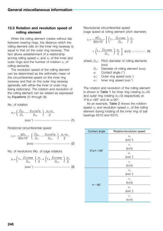
248


12.3 Rotation and revolution speed of rolling element

When the rolling element rotates without slip between bearing rings, the distance which the rolling element rolls on the inner ring raceway is equal to that on the outer ring raceway. This fact allows establishment of a relationship among rolling speed ni and ne of the inner and outer rings and the number of rotation na of rolling elements.

The revolution speed of the rolling element can be determined as the arithmetic mean of the circumferential speed on the inner ring raceway and that on the outer ring raceway (generally with either the inner or outer ring being stationary). The rotation and revolution of the rolling element can be related as expressed by Equations (1) through (4).

No. of rotation

na= –

(min–1) ......................................... (1)

Rotational circumferential speed

va= –

(m/s) ......................................... (2)

No. of revolutions (No. of cage rotation)

nc= 1– + 1+

(min–1) ......................................... (3)

Revolutional circumferential speed(cage speed at rolling element pitch diameter)

vc= 1–

+ 1+ (m/s) ................ (4)

where, Dpw: Pitch diameter of rolling elements (mm)

Dw: Diameter of rolling element (mm) a: Contact angle (° ) ne: Outer ring speed (min–1) ni: Inner ring speed (min–1)

The rotation and revolution of the rolling element is shown in Table 1 for inner ring rotating (ne=0) and outer ring rotating (ni=0) respectively at 0°≦ a <90° and at a=90°.

As an example, Table 2 shows the rotation speed na and revolution speed nc of the rolling element during rotating of the inner ring of ball bearings 6210 and 6310.

Dpw

Dw

Dwcos2aDpw

ne–ni

2( )

pDw

60´103

Dpw

Dw

Dwcos2aDpw

ne–ni

2( )

DwcosaDpw

ni

2( ) DwcosaDpw

ne

2( )

pDpw

60´103

DwcosaDpw

ni

2( )[

]DwcosaDpw

ne

2( )

Contact angle Rotation/revolution speed

0°≦ a＜90°

na

(min−1)

va

(m/s)

nc

(min−1)

vc

(m/s)

a＝90°

na

(min−1)

va

(m/s)

nc

(min−1)

vc

(m/s)

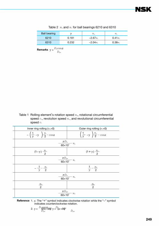
248 249

　　　　　　 Dwcos aRemarks　γ =――――　　　　　　　　Dpw

Table 2 na and nc for ball bearings 6210 and 6310

Ball bearing γ na nc

6210 0.181 −2.67ni 0.41ni

6310 0.232 −2.04ni 0.38ni

Table 1 Rolling element,s rotation speed na, rotational circumferential

speed va, revolution speed nc, and revolutional circumferentialspeed vc

Reference 1. ±: The “＋” symbol indicates clockwise rotation while the “−” symbol indicates counterclockwise rotation. Dwcosa ――――――――Dw2. γ =―――― (0°―a <90°), γ =――― (a =90°) Dpw Dpw

Inner ring rolling (ne=0) Outer ring rolling (ni=0)

−　── −γ 　──・cosa 　── −γ 　──・cosa

───── na

(1−γ ) ── (1＋γ ) ──

───── nc

− ──・── ─・──

───── na

── ──

───── nC

1γ

ni

2( ) 1γ

ne

2( )p Dw

60×103

ni

2ne

2

p Dpw

60×103

1γ

ni

21γ

ne

2

p Dw

60×103

ni

2ne

2

p Dpw

60×103

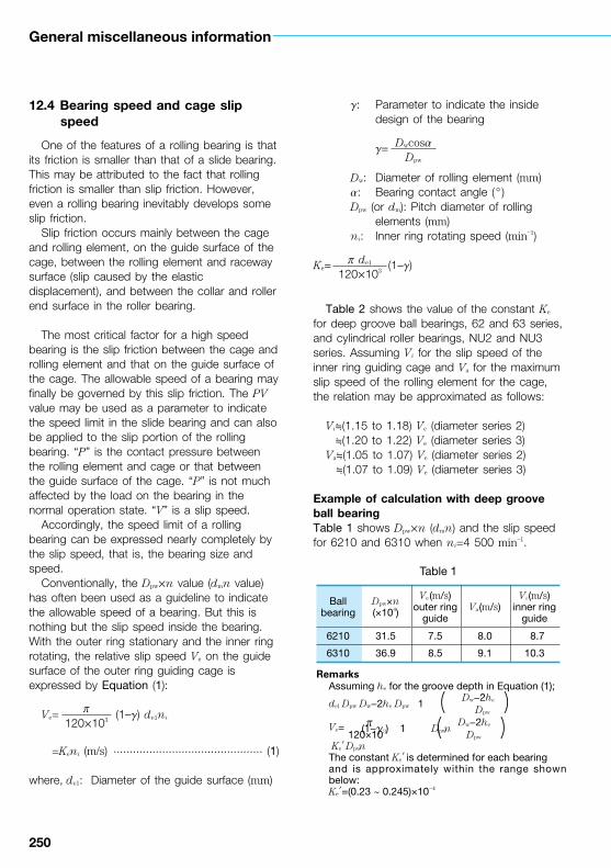
250


12.4 Bearing speed and cage slip speed

One of the features of a rolling bearing is that its friction is smaller than that of a slide bearing. This may be attributed to the fact that rolling friction is smaller than slip friction. However, even a rolling bearing inevitably develops some slip friction.

Slip friction occurs mainly between the cage and rolling element, on the guide surface of the cage, between the rolling element and raceway surface (slip caused by the elastic displacement), and between the collar and roller end surface in the roller bearing.

The most critical factor for a high speed bearing is the slip friction between the cage and rolling element and that on the guide surface of the cage. The allowable speed of a bearing may finally be governed by this slip friction. The PV value may be used as a parameter to indicate the speed limit in the slide bearing and can also be applied to the slip portion of the rolling bearing. “P” is the contact pressure between the rolling element and cage or that between the guide surface of the cage. “P” is not much affected by the load on the bearing in the normal operation state. “V” is a slip speed.

Accordingly, the speed limit of a rolling bearing can be expressed nearly completely by the slip speed, that is, the bearing size and speed.

Conventionally, the Dpw´n value (dmn value) has often been used as a guideline to indicate the allowable speed of a bearing. But this is nothing but the slip speed inside the bearing. With the outer ring stationary and the inner ring rotating, the relative slip speed Ve on the guide surface of the outer ring guiding cage is expressed by Equation (1):

Ve= (1–γ) de1ni

=Keni (m/s) .............................................. (1)

where, de1: Diameter of the guide surface (mm)

γ: Parameter to indicate the inside design of the bearing

γ=

Dw: Diameter of rolling element (mm) a: Bearing contact angle (° ) Dpw (or dm): Pitch diameter of rolling

elements (mm) ni: Inner ring rotating speed (min–1)

Ke= (1–γ)

Table 2 shows the value of the constant Ke for deep groove ball bearings, 62 and 63 series, and cylindrical roller bearings, NU2 and NU3 series. Assuming Vi for the slip speed of the inner ring guiding cage and Va for the maximum slip speed of the rolling element for the cage, the relation may be approximated as follows:

Vi≒(1.15 to 1.18) Ve (diameter series 2)≒(1.20 to 1.22) Ve (diameter series 3)

Va≒(1.05 to 1.07) Ve (diameter series 2)≒(1.07 to 1.09) Ve (diameter series 3)

Example of calculation with deep groove ball bearingTable 1 shows Dpw´n (dmn) and the slip speed for 6210 and 6310 when ni=4 500 min–1.

p120´103

DwcosaDpw

p de1

120´103

Table 1

Ball bearing

Dpw×n(×104)

Ve(m/s)outer ring

guideVa(m/s)

Vi(m/s)inner ring

guide

6210 31.5 7.5 8.0 8.7

6310 36.9 8.5 9.1 10.3

RemarksAssuming he for the groove depth in Equation (1); Dw−2hedel―Dpw―Dw−2he―Dpw 1――――― Dpw

p Dw−2heVe=――――― (1−γ ) 1――――― Dpw―n 120×103 Dpw

―Ke′―Dpw―nThe constant Ke′ is determined for each bearingand is approximately within the range shown below:Ke′=(0.23 ~ 0.245)×10−4

( )( )

250 251

Table 2 Constant Ke for 62 and 63 series ball bearings and NU2 and NU3 series roller bearings

Bearing bore No.

Bearing series

62 63 NU2 NU3

―――――――×10−5 ―――――――×10−5 ―――――――×10−5 ―――――――×10−5

000102

030405

060708

091011

121314

151617

181920

212224

262830

323436

3840

48 50 59

67 77 92

110125142

155168184

206221233

249264281

298316334

350368400

430470510

550585607

642682

49 52 66

74 81103

121133149

171189201

218235252

270287305

323340366

379406441

475511551

585615655

695725

―――

― 79 92

110126144

157172189

208226239

251270288

304323341

361378408

441478515

551588615

651689

―――

― 84102

123136155

171189206

224259261

278298314

333352376

392416449

486523559

599635670

707747

252


12.5 Centrifugal force of rolling elements

Under normal operating conditions, the centrifugal force on a rolling element is negligible when compared with the load on the bearing and thus not taken into account during calculation of the effective life of the bearing. However, if the bearing is running at high speed, then even if the load is small, the effect of the centrifugal force on the rolling element cannot be ignored. The deep groove ball bearing and cylindrical roller bearing suffer a decrease in the effective life because of the centrifugal force on the rolling element. In the case of an angular contact ball bearing, the contact angle of the inner ring increases and that of the outer ring decreases from the initial value, resulting in relative variation in the fatigue probability.

Apart from details of the effect on the life, the centrifugal force Fc of the rolling element during rotating of the inner ring is expressed by Equations (1) and (2) respectively for a ball bearing and roller bearing.

Ball bearing

Fc=KBni2 ......................................................... (1)

KB=5.580´10–12Dw3Dpw (1–γ)2 ......................... (N)

=0.569´10–12Dw3Dpw (1–γ)2 ...................... {kgf}

Roller bearing

Fc=KRni2 ......................................................... (2)

KR=8.385´10–12Dw2LwDpw (1–γ)2

....................................... (N)=0.855´10–12Dw

2LwDpw (1–γ)2

.................................... {kgf}

where, Dw: Diameter of roller element (mm) Dpw: Pitch diameter of rolling elements

(mm) γ: Parameter to indicate the internal

design of the bearing

γ=

a: Contact angle of bearing (° ) Lw: Length of roller (mm) ni: Inner ring rotating speed (min–1)

Table 1 shows the K values (KB and KR) for both series of NU2 & NU3 roller bearings and the 62 & 63 ball bearings.

DwcosaDpw

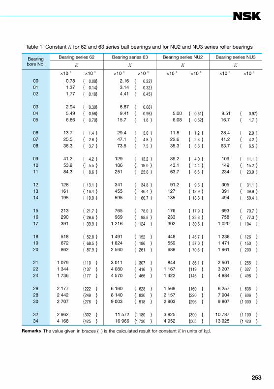
252 253

Table 1 Constant K for 62 and 63 series ball bearings and for NU2 and NU3 series roller bearings

Bearingbore No.

Bearing series 62 Bearing series 63 Bearing series NU2

K K K

×10−8 ×10−8 ×10−8 ×10−8 ×10−8 ×10−8

000102

030405

060708

091011

121314

151617

181920

212224

262830

3234

0.781.371.77

2.945.496.86

13.725.536.3

41.253.984.3

128161195

213290391

518672862

1 0791 3441 736

2 1772 4422 707

2 9624 168

{ 0.08}{ 0.14}{ 0.18}

{ 0.30}{ 0.56}{ 0.70}

{ 1.4 }{ 2.6 }{ 3.7 }

{ 4.2 }{ 5.5 }{ 8.6 }

{ 13.1 }{ 16.4 }{ 19.9 }

{ 21.7 }{ 29.6 }{ 39.9 }

{ 52.8 }{ 68.5 }{ 87.9 }

{110 }{137 }{177 }

{222 }{249 }{276 }

{302 }{425 }

2.163.144.41

6.679.41

15.70

29.4047.1073.50

129 186 251

341 455 595

765 9691 216

1 4911 8242 560

3 0114 0804 570

6 1608 1409 003

11 572――16 966――

{ 0.22}{ 0.32}{ 0.45}

{ 0.68}{ 0.96}{ 1.6 }

{ 3.0 }{ 4.8 }{ 7.5 }

{ 13.2 }{ 19.0 }{ 25.6 }

{ 34.8 }{ 46.4 }{ 60.7 }

{ 78.0 }{ 98.8 }

{ 124 }

{ 152 }{ 186 }{ 261 }

{ 307 }{ 416 }{ 466 }

{ 628 }{ 830 }{ 918 }

{1 180 }{1 730 }

―――

―5.006.08

11.822.635.3

39.243.163.7

91.2127135

176233302

448559689

8441 1671 422

1 5692 1572 903

3 8254 952

{ 0.51}{ 0.62}

{ 1.2 }{ 2.3 }{ 3.6 }

{ 4.0 }{ 4.4 }{ 6.5 }

{ 9.3 }{ 12.9 }{ 13.8 }

{ 17.9 }{ 23.8 }{ 30.8 }

{ 45.7 }{ 57.0 }{ 70.3 }

{ 86.1 }{119 }{145 }

{160 }{220 }{296 }

{390 }{505 }

Bearing series NU3

K

×10−8 ×10−8

―――

―――― 9.51―― 16.7

―― 28.4―― 41.2―― 63.7

109 149 234

305 391 494

693 7581 020

1 2361 4711 961

2 5013 2074 884

6 2577 9049 807

10 78713 925

{ 0.97}{ 1.7 }

{ 2.9 }{ 4.2 }{ 6.5 }

{ 11.1 }{ 15.2 }{ 23.9 }

{ 31.1 }{ 39.9 }{ 50.4 }

{ 70.7 }{ 77.3 }{ 104 }

{ 126 }{ 150 }{ 200 }

{ 255 }{ 327 }{ 498 }

{ 638 }{ 806 }{1 000 }

{1 100 }{1 420 }

Remarks　The value given in braces { } is the calculated result for constant K in units of kgf.

254


12.6 Temperature rise and dimensional change

Rolling bearings are extremely precise mechanical elements. Any change in dimensional accuracy due to temperature cannot be ignored. Accordingly, it is specified as a rule that measurement of a bearing must be made at 20°C and that the dimensions to be set forth in the standards must be expressed by values at 20°C.

Dimensional change due to temperature change not only affects the dimensional accuracy, but also causes change in the internal clearance of a bearing during operation. Dimensional change may cause interference between the inner ring and shaft or between the outer ring and housing bore. It is also possible to achieve shrink fitting with large interference by utilizing dimensional change induced by temperature difference. The dimensional change Dl due to temperature rise can be expressed as in Equation (1) below:

Dl=DT a l (mm) ...................................... (1)

where, Dl: Dimentional change (mm) DT: temperature rise (°C) a: Coefficient of linear expansion for

bearing steel a=12.5´10–6 (1/°C) l: Original dimension (mm)

Equation (1) may be illustrated as shown in Fig. 1. In the following cases, Fig. 1 can be utilized to easily obtain an approximate numerical values for dimensional change:

(1) To correct dimensional measurements according to the ambient air temperature

(2) To find the change in bearing internal clearance due to temperature difference between inner and outer rings during operation

(3) To find the relationship between the interference and heating temperature during shrink fitting

(4) To find the change in the interference when a temperature difference exists on the fit surface

ExampleTo what temperature should the inner ring be heated if an inner ring of 110 mm in bore is to be shrink fitted to a shaft belonging to the n6 tolerance range class?

The maximum interference between the n6 shaft of 110 in diameter and the inner ring is 0.065. To enable insertion of the inner ring with ease on the shaft, there must be a clearance of 0.03 to 0.04. Accordingly, the amount to expand the inner ring must be 0.095 to 0.105.Intersection of a vertical axis Dl=0.105 and a horizontal axis l=110 is determined on a diagram. DT is located in the temperature range between 70°C and 80°C (DT≒77°C). Therefore, it is enough to set the inner ring heating temperature to the room temperature +80°C.

254 255

Fig. 1　Temperature rise and dimensional change of bearing steel

256


12.7 Bearing volume and apparent specific gravity

The bearing bore is expressed by “d” (mm), the bearing outside diameter by “D” (mm), and the width by “B” (mm). The volume “V” of a bearing is expressed as follows:

V= (D2–d2) B´10–3 (cm3) ........................ (1)

Table 1 shows the bearing volume for the principal dimension series of radial bearings. In the case of a tapered roller bearing, the volume is a calculated value assuming the assembly width as “B”. When the bearing mass is expressed by “W” (kg), W/V=k may be considered as an apparent specific gravity and the value of “k” is nearly constant according to the type of bearings.

Table 2 shows the values of “k” for radial bearings of each dimension series. When the mass of a bearing not included in the standard dimension series is to be determined, the approximate mass value may be known by using the apparent specific gravity “k” if the bearing volume “V” has been determined.

p4

Bearingbore No.

Radial bearing

10 30

000102

030405

060708

091011

121314

151617

181920

212224

262830

3.64.05.4

7.412.914.9

21.728.835.6

45.249.071.7

76.781.6

113

119159175

217226236

298369396

598632773

5.46.07.9

10.317.120.0

31.741.150.0

65.070.5

104

111118170

179239270

334348362

469594649

9451 0201 240

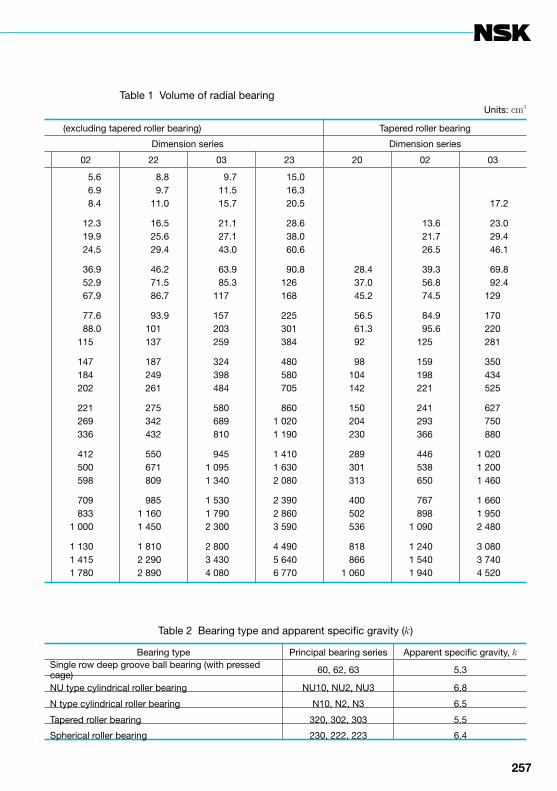
256 257

Table 1 Volume of radial bearingUnits: cm3

(excluding tapered roller bearing) Tapered roller bearing

Dimension series Dimension series

02 22 03 23 20 02 03

5.66.98.4

12.319.924.5

36.952.967.9

77.688.0

115

147184202

221269336

412500598

709833

1 000

1 1301 4151 780

8.89.7

11.0

16.525.629.4

46.271.586.7

93.9101137

187249261

275342432

550671809

9851 1601 450

1 8102 2902 890

9.711.515.7

21.127.143.0

63.985.3

117

157203259

324398484

580689810

9451 0951 340

1 5301 7902 300

2 8003 4304 080

15.016.320.5

28.638.060.6

90.8126168

225301384

480580705

8601 0201 190

1 4101 6302 080

2 3902 8603 590

4 4905 6406 770

―――

―――

28.437.045.2

56.561.392

98104142

150204230

289301313

400502536

818866

1 060

―――

13.621.726.5

39.356.874.5

84.995.6

125

159198221

241293366

446538650

767898

1 090

1 2401 5401 940

――17.2

23.029.446.1

69.892.4

129

170220281

350434525

627750880

1 0201 2001 460

1 6601 9502 480

3 0803 7404 520

Table 2 Bearing type and apparent specific gravity (k)

Bearing type Principal bearing series Apparent specific gravity, kSingle row deep groove ball bearing (with pressed cage) 60, 62, 63 5.3

NU type cylindrical roller bearing NU10, NU2, NU3 6.8

N type cylindrical roller bearing N10, N2, N3 6.5

Tapered roller bearing 320, 302, 303 5.5

Spherical roller bearing 230, 222, 223 6.4

258


12.8 Projection amount of cage in tapered roller bearing

The cage of a tapered roller bearing is made of a steel plate press construction and projects perpendicularly from the side of the outer ring as shown in Fig. 1. It is essential to design the bearing mounting to prevent the cage from contacting such parts as the housing and spacer. It is also recommended to employ the dimension larger than specified in JIS B 1566 “Mounting Dimensions and Fit for Rolling Bearing” and Sa and Sb of the bearing catalog in view of securing the grease retaining space in the case of grease lubrication and in view of improving the oil flow in the case of oil lubrication.

However, if the dimension cannot be designed smaller due to a dimensional restriction in the axial direction, then mounting dimensions Sa and Sb should be selected by adding as large as possible space to the maximum projection values d1 and d2 (Table 1) to the cage from the outer ring side.

Fig. 1　Projection of a cage

Fig. 2　Dimensions related to bearing mounting

Bearingbore No.

HR329J HR320XJ

d1 d2 d1 d2

020304

/2205/28

06/3207

080910

111213

141516

17181920

―――

―――

――

1.3

1.9――

1.92.3

―

2.5――

―3.43.33.4

―――

―――

――

2.7

2.9――

3.33.5

―

4.1――

―5.55.25.1

――

1.5

1.61.91.9

2.02.02.5

2.32.93.0

3.13.12.5

2.93.54.5

4.24.44.54.5

――

2.9

3.13.53.5

3.13.93.7

4.24.74.6

5.15.05.9

5.65.57.2

6.57.27.17.1

258 259

Table 1 Projection of a cage of tapered roller bearingUnits: mm

―――――――――――――――Bearing series

HR330J HR331J HR302J HR322J HR332J HR303J HR303DJ HR323J

d1 d2 d1 d2 d1 d2 d1 d2 d1 d2 d1 d2 d1 d2 d1 d2

―――

―2.0

―

2.0―

2.2

2.2―

2.4

2.92.93.0

3.53.5

―

3.7―――

―――

―3.1

―

4.0―

3.4

3.2―

4.4

4.85.15.1

5.55.4

―

6.0―――

―――

―――

―――

―3.33.3

3.3――

―――

4.84.8

―3.8

―――

―――

―――

―4.75.1

6.3――

―――

7.67.5

―8.8

―0.71.0

―0.81.4

1.40.72.0

1.11.81.8

2.71.23.9

3.33.93.1

3.13.63.53.2

―2.02.9

―2.93.4

3.43.33.1

4.73.95.5

4.85.94.8

5.35.35.5

6.35.15.96.9

―0.30.6

0.90.91.5

1.51.61.7

1.41.91.7

2.13.42.8

2.72.83.1

2.12.61.92.0

―3.03.5

3.83.83.4

3.32.84.3

5.15.16.2

4.54.24.0

5.04.74.6

5.85.15.45.6

―――

―2.01.8

2.12.22.6

3.13.73.3

3.53.94.9

5.55.04.7

4.6――

3.8

―――

―3.33.8

4.64.44.7

5.56.05.8

6.67.07.4

7.07.97.6

8.7――

9.4

1.21.40.9

1.11.61.5

2.1―

2.9

1.82.52.2

2.63.13.1

3.23.02.2

3.4―――

3.33.73.7

2.93.44.8

3.9―

4.8

4.95.15.9

5.76.56.2

6.57.67.8

8.5―――

―――

―――

――

2.1

2.02.33.7

3.33.23.9

3.83.73.4

4.03.23.0

―

―――

―――

――

4.8

5.0 5.5 6.8

6.0 8.010.0

8.2 8.6 9.2

10.3 9.610.3

―

――

1.3

―1.5

―

1.6―

1.1

0.52.01.5

1.82.72.3

2.11.82.2

2.82.1

―2.1

――

3.2

― 4.5

―

4.0―

4.1

4.5 5.2 5.7

6.4 6.5 7.4

7.2 7.7 7.9

9.8 8.9

―10.3

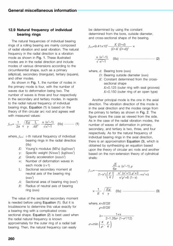
260


12.9 Natural frequency of individual bearing rings

The natural frequencies of individual bearing rings of a rolling bearing are mainly composed of radial vibration and axial vibration. The natural frequency in the radial direction is a vibration mode as shown in Fig. 1. These illustrated modes are in the radial direction and include modes of various dimensions according to the circumferential shape, such as a primary (elliptical), secondary (triangular), tertiary (square), and other modes.

As shown in Fig. 1, the number of nodes in the primary mode is four, with the number of waves due to deformation being two. The number of waves is three and four respectively in the secondary and tertiary modes. In regards to the radial natural frequency of individual bearing rings, Equation (1) is based on the theory of thin circular arc rod and agrees well with measured values:

fRiN= (Hz) ........... (1)

where, fRiN: ith natural frequency of individual bearing rings in the radial directios (Hz)

E: Young’s modulus (MPa) {kgf/mm2} γ: Specific weight (N/mm3) {kgf/mm3} g: Gravity acceleration (mm/s2) n: Number of deformation waves in

each mode (i+1) Ix: Sectional secondary moment at

neutral axis of the bearing ring (mm4)

A: Sectional area of bearing ring (mm2) R: Radius of neutral axis of bearing

ring (mm)

The value of the sectional secondary moment is needed before using Equation (1). But it is troublesome to determine this value exactly for a bearing ring with a complicated crosssectional shape. Equation (2) is best used when the radial natural frequency is known approximately for the outer ring of a radial ball bearing. Then, the natural frequency can easily

be determined by using the constant determined from the bore, outside diameter, and crosssectional shape of the bearing.

fRiN=9.41´105 ´

(Hz) ...................................... (2)

where, d: Bearing bore (mm) D: Bearing outside diameter (mm) K: Constant determined from the cross

sectional shape K=0.125 (outer ring with seal grooves) K=0.150 (outer ring of an open type)

Another principal mode is the one in the axial direction. The vibration direction of this mode is in the axial direction and the modes range from the primary to tertiary as shown in Fig. 2. The figure shows the case as viewed from the side. As in the case of the radial vibration modes, the number of waves of deformation in primary, secondary, and tertiary is two, three, and four respectively. As for the natural frequency of individual bearing rings in the axial direction, there is an approximation Equation (3), which is obtained by synthesizing an equation based upon the theory of circular arc rods and another based on the nonextension theory of cylindrical shells:

n (n2–1) rfAiN=

(1–ν2) 2 +n2+l

´ (Hz) ................................... (3)

where,κ=H/2R r=B/2R

l=

s=min ,

12p

Egγ

Ix

AR4

n (n2–1)n2–1

K (D–d){D–K (D–d)}2

√———

n (n2–1)n2–1√———

√—3

6pn2 (n2+1) r2+3n2r2+6 (1–ν)

1R

Egγ

1+ν2–1.26s (1–s4/12)

( )r

rr

κ

( )κκ

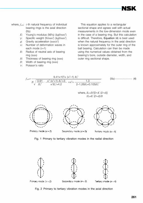
260 261

where, fAiN: ith natural frequency of individual bearing rings is the axial direction (Hz)

E: Young’s modulus (MPa) {kgf/mm2} γ: Specific weight (N/mm3) {kgf/mm3} g: Gravity acceleration (mm/s2) n: Number of deformation waves in

each mode (i+1) R: Radius of neutral axis of bearing

ring (mm) H: Thickness of bearing ring (mm) B: Width of bearing ring (mm)　 ν: Poisson’s ratio

This equation applies to a rectangular sectional shape and agrees well with actual measurements in the lowdimension mode even in the case of a bearing ring. But this calculation is difficult. Therefore, Equation (4) is best used when the natural frequency in the axial direction is known approximately for the outer ring of the ball bearing. Calculation can then be made using the numerical values obtained from the bearing’s bore, outside diameter, width, and outer ring sectional shape.

where, R0=B/{D–K (D–d)} H0=K (D–d)/B

fAiN= (Hz) ....................... (4)B · +n2+ 0.91

H02

n2 (n2+1) R02+3

n2R02+4.2

1.32–1.26H0+0.105H0

5

9.41´105n (n2–1) R02

Fig. 1　Primary to tertiary vibration modes in the radial direction

Fig. 2　Primary to tertiary vibration modes in the axial direction

262


12.10 Vibration and noise of bearings

The vibration and noise occurring in a rolling bearing are very diverse. Some examples are shown in Table 1. This table shows the vibration and noise of bearings while classifying them roughly into those inherent in the bearing design which occur regardless of the present superb technology and those caused by other reasons, both are further subdivided into several groups. The boundaries among these groups, however, are not absolute. Although vibration and noise due to the bearing structure may be related to the magnitude of the bearing accuracy, nevertheless, vibration attributed to accuracy may not be eliminated completely by improving the accuracy, because there exists certain effects generated by the parts surrounding the bearing.

Arrows in the table show the relationship between the vibration and noise.

Generally, vibration and noise are in a causal sequence but they may be confused. Under normal bearing running conditions, however, around 1 kHz may be used as a boundary line to separate vibration from noise. Namely, by convention, the frequency range of about 1 kHz or less will be treated as vibration while that above this range will be treated as noise.

Typical vibration and noise, as shown in Table 1, have already been clarified as to their causes and present less practical problems. But the environmental changes as encountered these days during operation of a bearing have come to generate new kinds of vibration and noise. In particular, there are cases of abnormal noise in the low temperature environment, which can often be attributed to friction inside of a bearing. If the vibration and noise (including new kinds of abnormal noise) of a bearing are to be prevented or reduced, it is essential to define and understand the phenomenon by focusing on vibration and noise beforehand. As portable tape recorders with satisfactory performance are commonly available these days, it is recommended to use a tape recorder to record the actual sound of the vibration or noise.

Table 1 Vibration and noise of rolling bearing

Vibration inherentin bearing design

Vibration related tobearing accuracy

Vibration causedby faulty handlingof bearing

Passing vibrationof rolling element

Natural frequencyof bearing ring

Vibration causedby bearingelasticity

Vibration causedby waviness ofraceway or rollingsurface

Vibration of cage

Vibration due tonicks

Vibration due tocontamination

262 263

Bearing Vibration Noise

Angular natural frequencyof outer ring inertiamoment system

Axial natural frequency ofouter ring mass system

Bending natural frequencyof bearing ring

Axial vibration

Radial vibration

Resonant vibration aroundbearing

Race noise

Rolling elementdropping noise

Squealling noise

Humming noise

Bracket resonancenoise

Noise caused bywaviness ofraceway or rollingelement

Cage noise

Nick noise

Noise fromcontamination

Noise inherent in bearingconstruction

Noise generated afterbearing mounting

Noise related to bearingaccuracy

Noise caused by improperhandling of bearing

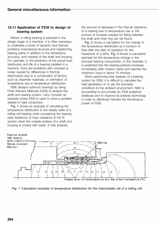
264


12.11 Application of FEM to design of bearing system

Before a rolling bearing is selected in the design stage of a machine, it is often necessary to undertake a study of dynamic and thermal problems (mechanical structure and neighboring bearing parts) in addition to the dimensions, accuracy, and material of the shaft and housing. For example, in the prediction of the actual load distribution and life of a bearing installed in a machine, there are problems with overload or creep caused by differences in thermal deformation due to a combination of factors such as dissimilar materials, or estimation of temperature rise or temperature distribution.

NSK designs optimum bearings by using Finite Element Methods (FEM) to analyze the shaft and bearing system. Let’s consider an example where FEM is used to solve a problem related to heat conduction.

Fig. 1 shows an example of calculating the temperature distribution in the steady state of a rolling mill bearing while considering the bearing heat resistance or heat resistance in the fit section when the outside surface of a shaft and housing is cooled with water. In this analysis,

the amount of decrease in the internal clearance of a bearing due to temperature rise or the amount of increase needed for fitting between the shaft and inner ring can be found.

Fig. 2 shows a calculation for the change in the temperature distribution as a function of time after the start of operation for the headstock of a lathe. Fig. 3 shows a calculation example for the temperature change in the principal bearing components. In this example, it is predicted that the bearing preload increases immediately after rotation starts and reaches the maximum value in about 10 minutes.

When performing heat analysis of a bearing system by FEM, it is difficult to calculate the heat generation or to set the boundary conditions to the ambient environment. NSK is proceeding to accumulate an FEM analytical database and to improve its analysis technology in order to effectively harness the tremendous power of FEM.

Fig. 1　Calculation example of temperature distribution for the intermediate roll of a rolling mill

264 265

Fig. 2　Calculation example of temperature rise in headstock of lathe

Fig. 3　Calculation example of temperature rise in bearing system

266


As an example of applying the FEMbased analysis, we introduce here the result of a study on the effect of the shape of a rocker plate supporting the housing of a plate rolling mill both on the life of a tapered roller bearing (f489´f635 in dia. ´321) and on the housing stress. Fig. 4 shows an approximated view of the housing and rocker plate under analysis. The following points are the rerults of analysis made while changing the relief amount l at the top surface of the rocker plate:

(1) The maximum value smax of the stress (maximum main stress) on a housing occurs at the bottom of the housing.

(2) smax increases with increase in l. But it is small relative to the fatigue limit of the material.

(3) The load distribution in the rolling element of the bearing varies greatly depending on l. The bearing life reaches a maximum at around l/L=0.7.

(4) In this example, l/L=0.5 to 0.7 is considered to be the most appropriate in view of the stress in the housing and the bearing life.Fig. 5 shows the result of calculation on the housing stress distribution and shape as well as the rolling element load distribution when l/L≒0.55.

Fig. 6 shows the result of a calculation on the housing stress and bearing life as a function of change in l.

FEMbased analysis plays a crucial role in the design of bearing systems. Finite Element Methods are applicable in widelyvarying fields as shown in Table 1. Apart from these, FEM is used to analyze individual bearing components and contribute to NSK’s highlevel bearing design capabilities and achievements. Two examples are the analysis of the strength of a rib of a roller bearing and the analysis of the natural mode of a cage.

Fig. 4　Rolling mill housing and rocker plate

Fig. 5　Calculation example of housing stress and rolling element load distribution of bearing

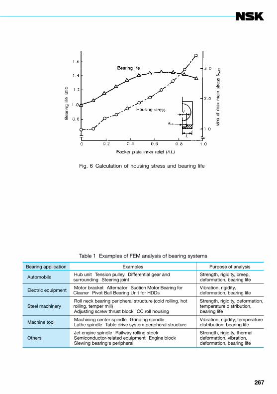
266 267

Fig. 6　Calculation of housing stress and bearing life

Table 1 Examples of FEM analysis of bearing systems

Bearing application Examples Purpose of analysis

Automobile―Hub unit ―Tension pulley ―Differential gear andsurrounding ―Steering joint

Strength, rigidity, creep,deformation, bearing life

Electric equipment―Motor bracket ―Alternator ―Suction Motor Bearing for Cleaner ―Pivot Ball Bearing Unit for HDDs

Vibration, rigidity,deformation, bearing life

Steel machinery―Roll neck bearing peripheral structure (cold rolling, hotrolling, temper mill)―Adjusting screw thrust block ―CC roll housing

Strength, rigidity, deformation,temperature distribution,bearing life

Machine tool―Machining center spindle ―Grinding spindle―Lathe spindle ―Table drive system peripheral structure

Vibration, rigidity, temperaturedistribution, bearing life

Others―Jet engine spindle ―Railway rolling stock―Semiconductor-related equipment ―Engine block―Slewing bearing,s peripheral

Strength, rigidity, thermaldeformation, vibration,deformation, bearing life

268

13. NSK special bearings

13.1 Ultra-precision ball bearings for gyroscopes

(1) Gyroscope bearingsGyroscopes are used to detect and

determine traveling position and angular velocity in airplanes and ships. Gyros are structurally divided into two groups depending on the number of directions and speeds of movement to be detected: those with one degree of freedom and those with two degrees of freedom. (See Fig. 1)The performance of a gyro depends on the characteristics of the bearing. Thus, a gyro bearing is required to demonstrate top grade performance among the ultra-precision miniature bearings. Gyros have two sets of bearings. One set supports the rotor shaft running at high speed and the other set supports the frame (gimbal). Both must have stable, low frictional torque. Principal types and application environments of rolling bearings for gyros are shown in Table 1.

The inch series of ultra-precision bearings are almost exclusively used for rotors and gimbals. Boundary dimensions and typical NSK bearing numbers are shown in Table 2.

Special-shaped bearings dedicated to gyro applications are also used in large quantity.

Table 1 Type and running conditions of gyro bearings

Application Principal bearing type Typical running conditions

RotorAngular contact ball bearingEnd-cap ball bearing

12 000, 24 000 min−1 or 36 000 min−1, 60 to 80°Chelium gas

GimbalDeep groove ball bearingOther special-shaped bearings

Oscillation within ±2°,Normal temperatures to 80°C,Silicon oil or air

268 269

Fig. 1　Gyro type

270

NSK special bearings

*　Angular contact type bearing is also available for rotor.

Table 2 Boundary dimensions and bearing number of gyroscope bearings

Boundary dimensions (mm) Bearing numbers

d D B B1 r(min.)

Open Both-sideshielded

1.0161.1911.397

1.9842.380

3.175

3.967

4.762

6.350

7.9389.525

3.175 3.967 4.762

6.350 4.762 4.762 7.938

6.350 7.938 9.525

9.52512.700 7.938

7.938 9.52512.700

9.52512.70015.87519.050

12.70022.225

1.1911.5881.984

2.3801.588

　2.779

2.3802.7792.779

3.9674.3662.779

2.7793.1753.967

3.1753.1754.9785.558

3.9675.558

　2.3802.779

3.571　

2.3803.571

2.7793.5713.571

3.9674.3663.175

3.1753.1754.978

3.1754.7624.9787.142

3.9677.142

0.10.10.1

0.10.10.10.15

0.10.10.15

0.30.30.1

0.10.10.3

0.10.150.30.4

0.150.4

R 09R 0

*R 1

*R 1-4*R 133

　*R 1-5

*R 144R 2-5

*R 2-6

*R 2R 2 AR 155

R 156R 166

*R 3

R 168 BR 188

*R 4 B*R 4 AA

R 1810R 6

　R 0 ZZR 1 ZZ

R 1-4 ZZ

　R 133 ZZSR 1-5 ZZ

R 144 ZZR 2-5 ZZR 2-6 ZZS

R 2 ZZR 2 AZZR 155 ZZS

R 156 ZZSR 166 ZZR 3 ZZ

R 168 BZZR 188 ZZR 4 BZZR 4 AAZZ

R 1810 ZZR 6 ZZ

270 271

Boundary dimensions (mm) Bearing numbers

D1 C1 C2 Open,with flange

Both-side shielded,with flange

　 5.156 5.944

7.518 5.944 5.944 9.119

7.518 9.11910.719

11.176　

9.119

9.11910.71914.351

10.71913.89417.526

　

13.89424.613

　0.3300.580

0.5800.460

　0.580

0.5800.5800.580

0.760　

0.580

0.5800.5801.070

0.5800.5801.070

　

0.7901.570

　0.7900.790

0.790　

0.7900.790

0.7900.7900.790

0.760　

0.910

0.9100.7901.070

0.9101.1401.070

　

0.7901.570

　FR 0FR 1

FR 1-4FR 133

　FR 1-5

FR 144FR 2-5FR 2-6

FR 2　

FR 155

FR 156FR 166FR 3

FR 168 BFR 188FR 4 B

　

FR 1810FR 6

　FR 0 ZZFR 1 ZZ

FR 1-4 ZZ

　FR 133 ZZSFR 1-5 ZZ

FR 144 ZZFR 2-5 ZZFR 2-6 ZZS

FR 2 ZZ

　FR 155 ZZS

FR 156 ZZSFR 166 ZZFR 3 ZZ

FR 168 BZZFR 188 ZZFR 4 BZZ

　

FR 1810 ZZFR 6 ZZ

272


(2) Characteristics of gyroscope bearings(2.1) Rotor bearing

The rotor bearing is required to offer extremely-low, torque at high speed, and free from variation and long term stability. To meet these demands, the bearing uses an oil-immersed cage in most cases. A lubrication method of injecting the lubricating oil dissolved with solvent into a bearing is also available, but this method requires adequate concentration adjustment because the frictional torque is affected by the oil amount (Fig. 2). In such an event, the oil amount is adjusted through centrifugal separation to obtain variation-free running torque. A special bearing type, in which an end cap is integrated with the outer ring, may also be used (Fig. 3).

(2.2) Gimbal bearingRequirements on the gimbal bearing as a

gyro output axis include low frictional torque and vibration resistance. Table 3 shows the

maximum starting frictional torque for typical bearings. Much smaller starting torque can be obtained through precision machining of the raceway groove and special design of the cage.

Fig. 3　Typical end-cap ball bearing

Fig. 2　Oil amount and running torque

272 273

Table 4 Specifications of bearings for rotors and gimbals

Item Rotor bearing Gimbal bearing

Bearing type

Bearing accuracy

Lubricationmethod

Cage

Ball accuracy

Bearing contactangle ( °)

Angular contact ball

CLASS 7P or above

Oil-immersed cage and self-lubrication (dual use greaseavailable)

Laminated phenol

Around Grade 3

20 to 28

Deep groove ball or angularcontact ball

CLASS 5P or CLASS 7P

Oil lubrication, filled with anadequate quantity

Steel sheet (low torque design)

Around Grade 5 or above

　

Table 3 Maximum starting torque

BearingNo.

Measuring load

mN {gf}

Radial internal clearance (μm)

MC23 to 8

MC35 to 10

MC48 to 13

MC513 to 20

MC620 to 28

Maximum starting torque (μN　m) {mgf　mm}

R1

R1-5

R144

R2

R3

R4B

735{75}

735{75}

735{75}

735{75}

3 900{400}

3 900{400}

7.95{810}

13.2{1 350}

8.92{910}

14.7{1 500}

63.5{6 500}

68.5{7 000}

7.35{750}

12.3{1 250}

8.35{840}

13.7{1 400}

54.0{5 500}

59.0{6 000}

6.75{690}

11.8{1 200}

7.65{780}

12.7{1 300}

54.0{5 500}

59.0{6 000}

6.10{620}

10.7{1 090}

6.85{700}

11.8{1 200}

49.0{5 000}

54.0{5 500}

5.20{530}

9.70{990}

6.08{620}

11.4{1 160}

44.0{4 500}

49.0{5 000}

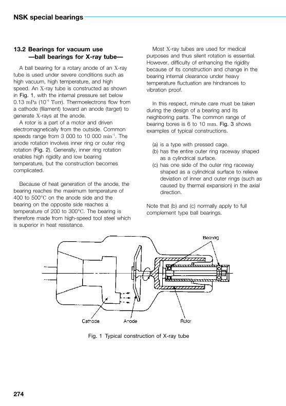
274


13.2 Bearings for vacuum use —ball bearings for X-ray tube—

A ball bearing for a rotary anode of an X-ray tube is used under severe conditions such as high vacuum, high temperature, and high speed. An X-ray tube is constructed as shown in Fig. 1, with the internal pressure set below 0.13 mPa (10–6 Torr). Thermoelectrons flow from a cathode (filament) toward an anode (target) to generate X-rays at the anode.

A rotor is a part of a motor and driven electromagnetically from the outside. Common speeds range from 3 000 to 10 000 min–1. The anode rotation involves inner ring or outer ring rotation (Fig. 2). Generally, inner ring rotation enables high rigidity and low bearing temperature, but the construction becomes complicated.

Because of heat generation of the anode, the bearing reaches the maximum temperature of 400 to 500°C on the anode side and the bearing on the opposite side reaches a temperature of 200 to 300°C. The bearing is therefore made from high-speed tool steel which is superior in heat resistance.

Most X-ray tubes are used for medical purposes and thus silent rotation is essential. However, difficulty of enhancing the rigidity because of its construction and change in the bearing internal clearance under heavy temperature fluctuation are hindrances to vibration proof.

In this respect, minute care must be taken during the design of a bearing and its neighboring parts. The common range of bearing bores is 6 to 10 mm. Fig. 3 shows examples of typical constructions.

(a) is a type with pressed cage.(b) has the entire outer ring raceway shaped

as a cylindrical surface.(c) has one side of the outer ring raceway

shaped as a cylindrical surface to relieve deviation of inner and outer rings (such as caused by thermal expansion) in the axial direction.

Note that (b) and (c) normally apply to full complement type ball bearings.

Fig. 1　Typical construction of X-ray tube

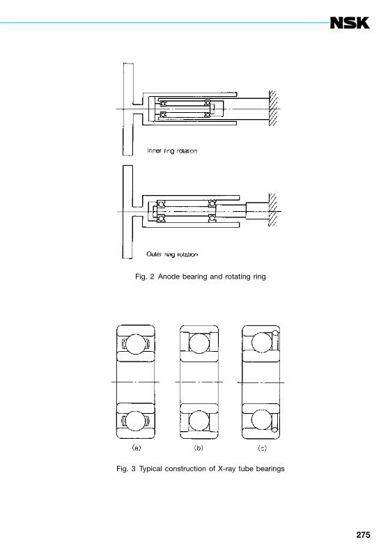
274 275

Fig. 2　Anode bearing and rotating ring

Fig. 3　Typical construction of X-ray tube bearings

276


One of the greatest challenges facing X-ray tube ball bearings is the lubrication method. Because of the vacuum and high temperature environment, a solid lubricant is used with one of the methods described below:(1) Provision of laminated solid lubrication (molybdenum disulfide) to the pocket surface of a cage(2) Provision of thin film of mild metal (silver or lead) over the surface of balls, inner ring/outer ring raceway

The method (2) above applies mostly to full-complement type ball bearings and the thin film is provided by plating, ion plating, etc. The results of a durability test performed on a ball bearing with a soft metal coating in a vacuum are shown in Fig. 4. By the way, Fig. 4 shows a comparison of the endurance time for different conditions of ball bearings (8 mm in bore and 22 mm in outside diameter) that are rotated at 9 000 min–1 under an axial load of 20 N {2 kgf} at 0.13 mPa {10–6 Torr} while at room temperature. Fig. 5 shows a graph of the change in running torque as a function of time.

The raceway wear becomes substantial only when the balls are made of ceramics and there is no lubrication. However, if a lubrication film is provided for the raceway, then the torque variation becomes small and stable. Fig. 6 shows an example of a test with the housing temperature set at 300°C for a ball bearing of 9.5 mm in bore and 22 mm in outside diameter which rotates at 9 000 min–1 under an axial load of 5 N {0.5 kgf} or 20 N {2 kgf}.

　

　

0 50 100

Time, h

MaterialLubrication DurationInner/outer

ring Ball

Metal

Metal

a. No lubrication

b. Silver coated balls

c. Silver coated inner/ outer rings and balls

Ceramicsd. No lubrication

e. Silver coated inner/ outer rings

Fig. 4　Lubricating conditions and durable time (room temperature)

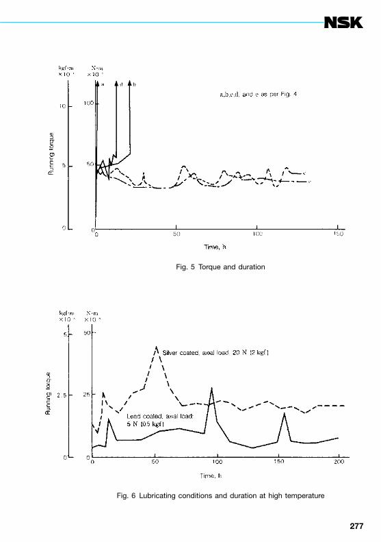
276 277

Fig. 5　Torque and duration

Fig. 6　Lubricating conditions and duration at high temperature

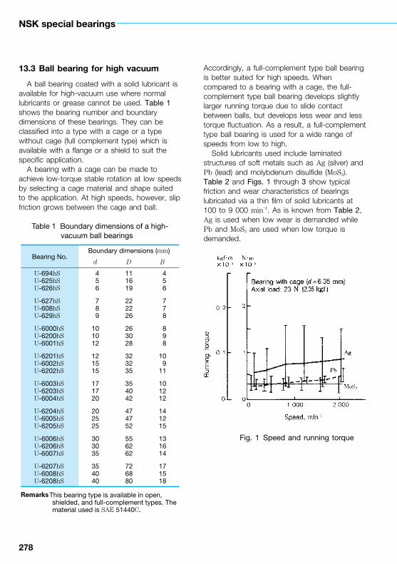
278


13.3 Ball bearing for high vacuum

A ball bearing coated with a solid lubricant is available for high-vacuum use where normal lubricants or grease cannot be used. Table 1 shows the bearing number and boundary dimensions of these bearings. They can be classified into a type with a cage or a type without cage (full complement type) which is available with a flange or a shield to suit the specific application.

A bearing with a cage can be made to achieve low-torque stable rotation at low speeds by selecting a cage material and shape suited to the application. At high speeds, however, slip friction grows between the cage and ball.

Accordingly, a full-complement type ball bearing is better suited for high speeds. When compared to a bearing with a cage, the full-complement type ball bearing develops slightly larger running torque due to slide contact between balls, but develops less wear and less torque fluctuation. As a result, a full-complement type ball bearing is used for a wide range of speeds from low to high.

Solid lubricants used include laminated structures of soft metals such as Ag (silver) and Pb (lead) and molybdenum disulfide (MoS2). Table 2 and Figs. 1 through 3 show typical friction and wear characteristics of bearings lubricated via a thin film of solid lubricants at 100 to 9 000 min–1. As is known from Table 2, Ag is used when low wear is demanded while Pb and MoS2 are used when low torque is demanded.

Table 1 Boundary dimensions of a high- vacuum ball bearings

Remarks　This bearing type is available in open, shielded, and full-complement types. The material used is SAE 51440C.

Bearing No.Boundary dimensions (mm)

d D B

U-694hSU-625hSU-626hS

U-627hSU-608hSU-629hS

U-6000hSU-6200hSU-6001hS

U-6201hSU-6002hSU-6202hS

U-6003hSU-6203hSU-6004hS

U-6204hSU-6005hSU-6205hS

U-6006hSU-6206hSU-6007hS

U-6207hSU-6008hSU-6208hS

4 5 6

7 8 9

101012

121515

171720

202525

303035

354040

111619

222226

263028

323235

354042

474752

556262

726880

4 5 6

7 7 8

8 9 8

10 911

101212

141215

131614

171518

Fig. 1　Speed and running torque

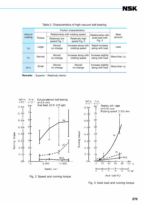
278 279

Remarks　　: Superior　　: Relatively inferior

Table 2 Characteristics of high-vacuum ball bearing

Kind ofcoating

Friction characteristics

WearamountTorque

Relationship with rotating speed Relationship withaxial load with

Fig. 3Relatively lowspeed Fig. 1

Relatively highspeed Fig. 2

Ag Large　

Almostno change

　

Increase along withrotating speed

　

Rapid increasealong with load

　

Less　

Pb Normal　

Almostno change

　

Increase along withrotating speed

　

Increase slightlyalong with load

　

More than Ag　

MoS2Small

　

Almostno change

　

Almostno change

　

Increase slightlyalong with load

　

More than Ag　

Fig. 2　Speed and running torque

Fig. 3　Axial load and running torque

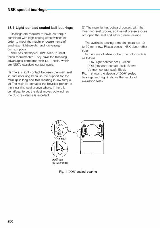
280


13.4 Light-contact-sealed ball bearings

Bearings are required to have low torque combined with high sealing effectiveness in order to meet the machine requirements of small-size, light-weight, and low-energy- comsumption.

NSK has developed DDW seals to meet these requirements. They have the following advantages compared with DDU seals, which are NSK’s standard contact seals.

(1) There is light contact between the main seal lip and inner ring because the support for the main lip is long and thin resulting in low torque.(2) The main lip contacts the bevelled portion of the inner ring seal groove where, if there is centrifugal force, the dust moves outward, so the dust resistance is excellent.

(3) The main lip has outward contact with the inner ring seal groove, so internal pressure does not open the seal and allow grease leakage.

The available bearing bore diameters are 10 to 50 mm now. Please consult NSK about other sizes.

In the case of nitrile rubber, the color code is as follows:

DDW (light-contact seal): GreenDDU (standard contact seal): BrownVV (non-contact seal): Black

Fig. 1 shows the design of DDW sealed bearings and Fig. 2 shows the results of evaluation tests.

Fig. 1　DDW sealed bearing

280 281

Fig. 2　Evaluation test results of DDW sealed bearings

282


13.5 Bearing with integral shaft

In consideration of the need for improved Audio-Visual (AV) and Office Automation (OA) equipment, bearings used in rotary mechanisms of small precision motors and so forth are increasingly demanded to demonstrate much higher performance. Enhanced quality of Video Cassette Recorders (VCR) and Digital Audio Terminals (DAT), increased density of Hard Disk Drives (HDD), and improved printing quality of Laser Beam Printers (LBP) have imposed severe requirements on equipment. These severe design requirements cover improvement of the runout accuracy (rotational repetitive runout, non-repetitive runout), low-noise, and reduction of power consumption as well as being easy-to-assemble. An NSK bearing with integral shaft is available and meets these exacting demands.

The bearing with integral shaft is a unit, which has no inner ring while having the raceway groove directly on the shaft to incorporate a preload spring between both outer rings (Fig. 1). This type of bearing has the following advantages over normal bearings:

(1) Improved recording/reproduction accuracy○Integration of the shaft and inner ring,

thereby eliminating movement of the shaft caused by fitting between the shaft and inner ring

○Thick-wall design of the outer ring as required, thereby reducing deformation of the outer ring due to interference

(2) Reduced power consumption of motor○Integration of the shaft and inner ring,

thereby reducing the ball pitch diameter for the same shaft diameter and resulting in a decrease of torque

(3) High shaft rigidity and compactness○Integration of the shaft and inner ring,

thereby reducing the bearing’s outside diameter for a given size shaft diameter.

(Example) 684ZZ: Shaft diameter 4 mm, outside diameter 9 mm (without shaft)

4BVD: Shaft diameter 4 mm, outside diameter 8 mm (with integral shaft)

(4) Aiming at “easy-to-assemble” designs○No parts are required for preload adjustment

and preloading○No need for selective fitting and adhesion

securing of the shaft and inner ringSpecifications on the NSK bearing with integral shaft are shown in Table 1.

282 283

Remarks　Consult NSK for the shaft length.

Table 1 Specifications on bearing with integral shaft

Boundary dimensions Basic load Ratings

(mm) (N) {kgf}

d D1 D2 W Cr Cor Cr Cor

345

678

6.4589

101315

7.051010

121517

3.544

456

435 550 640

710 9801 330

124173223

271365505

45 56 65

73100135

131823

283752

Fig. 1　Composition and runout accuracy of bearing with integral shaft

284


13.6 Bearings for electromagnetic clutches in car air-conditioners

The electromagnetic clutch is an important part and is necessary to activate the compressor of a car air-conditioner. The performance required of an electromagnetic clutch bearing differs depending on the type of compressor.Table 1 shows the relationship between the compressor type and the application conditions for electromagnetic clutch bearings.

Values shown in Table 1 are the maximum during practical operation. A bench test is made under more severe conditions to confirm the durability of the bearing.

The electromagnetic clutch bearing must prove durable under these conditions. Principal performances required of the bearing are listed below:○ Durability at high speed○ Durability at high temperature○ Bearing angular clearance should be kept

small to assure maintenance of a proper clearance between disk and armatureWhen deciding the bearing specifications, the

appropriateness of the following points should be considered:

○ Bearing internal design for high speed and longer life

○ Long-life grease for high temperatures and high speeds

○ Proper radial clearance○ Effective sealing system with low grease

leakage and superior in terms of dust proof and water proofMost of the bearings for electromagnetic

clutches have a bore in the range of 30 to 45 mm. One common arrangement is to use a pair of single-row deep groove ball bearings, and another is to use a double-row angular contact ball bearing.

A bearing for an electromagnetic clutch is required to have high speed, long grease life, proper internal clearance, and superior seal effectiveness. NSK bearings for electromagnetic clutches have the dimensions and features described below to meet the above performance requirements:

Fig. 1　Electromagnetic clutch for a reciprocating type compressor

Fig. 2　Electromagnetic clutch for axial type and rotary type compressors

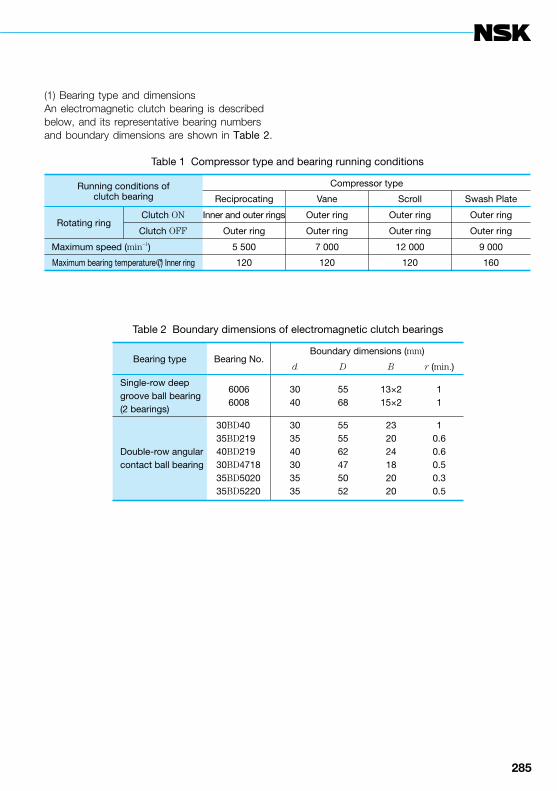
284 285

(1) Bearing type and dimensionsAn electromagnetic clutch bearing is described below, and its representative bearing numbers and boundary dimensions are shown in Table 2.

Table 2 Boundary dimensions of electromagnetic clutch bearings

Bearing type Bearing No.Boundary dimensions (mm)

d D B r (min.)

Single-row deepgroove ball bearing(2 bearings)

60066008

3040

5568

13×215×2

11

Double-row angularcontact ball bearing

30BD4035BD21940BD21930BD471835BD502035BD5220

303540303535

555562475052

232024182020

10.60.60.50.30.5

Table 1 Compressor type and bearing running conditions

Running conditions ofclutch bearing

Compressor type

Reciprocating Vane Scroll Swash Plate

Rotating ringClutch ON Inner and outer rings Outer ring Outer ring Outer ring

Clutch OFF Outer ring Outer ring Outer ring Outer ring

Maximum speed (min−1) 5 500 7 000 12 000 9 000

Maximum bearing temperature (°C) Inner ring 120 120 120 160

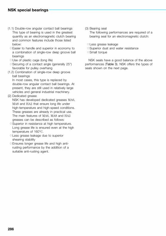
286


(1.1) Double-row angular contact ball bearingsThis type of bearing is used in the greatest quantity as an electromagnetic clutch bearing and common features include those listed below:

○ Easier to handle and superior in economy to a combination of single-row deep groove ball bearings

○ Use of plastic cage (long life)○ Securing of a contact angle (generally 25°)

favorable for pulley overhang(1.2) Combination of single-row deep groove

ball bearingsIn most cases, this type is replaced by double-row angular contact ball bearings. At present, they are still used in relatively large vehicles and general industrial machinery.

(2) Dedicated greaseNSK has developed dedicated greases MA6, MA8 and HA2 that ensure long life under high-temperature and high-speed conditions. These greases are already in practical use. The main features of MA6, MA8 and HA2 greases can be described as follows:

○ Superior in resistance at high temperature. Long grease life is ensured even at the high temperature of 160°C.

○ Less grease leakage due to superior shearing stability

○ Ensures longer grease life and high anti-rusting performance by the addition of a suitable anti-rusting agent.

(3) Bearing sealThe following performances are required of a bearing seal for an electromagnetic clutch:

○ Less grease leakage○ Superior dust and water resistance○ Small torque

NSK seals have a good balance of the above performances (Table 3). NSK offers the types of seals shown on the next page.

286 287

Table 3 Type and performance of NSK bearing seals

Seal performanceSeal type

DU DUK DUM

Grease leakage Fair Good Superior

Seal effectiveness(dust and water resistance) Fair Good Superior

Torque Good Good Good

Seal groove-seal lipcontact condition

Contact(with air hole)

Contact(without air hole)

Contact(without air hole)

288


13.7 Sealed clean bearings for transmissions

A sealed clean bearing for a transmission is a bearing with a special seal that can prevent entry of foreign matters into a gear box and thereby extend the fatigue life of a bearing substantially.

This type of bearing has proven in actual transmission endurance tests to have a durability life which is 6 to 10 times longer than that of standard ball bearings.

The special seal prevents harmful, extremely-small foreign matters suspended in the gear oil from entering the gear box. Thereby minimizing the number of dents and foreign matter that become embedded in the raceway. The bearing fatigue pattern is thus changed from a surface fatigue pattern to an internal fatigue pattern (a reference to be used in judgment of the bearing fatigue), which contributes to extension of the bearing life. This is not much affected by the recent trend to use low viscosity gear oil, either. In these respects, this kind of bearing is better than open type bearings.

Sealed clean bearings as described above are generally called transmission (TM) ball bearings. They are dedicated bearings for use in transmission applications and have the following major features:

1. Satisfactory design and specifications for a transmission bearing

2. Grease with an affinity for gear oil is filled to assist initial lubrication

3. The seal lip construction allows inflow of lubricating oil while preventing entry of foreign matters. (Fig. 1)

4. Lower torque when compared with normal contact seal bearingsThese TM ball bearings are produced as

series products as shown in Table 1. TM ball bearings have the same nominal dimensions as the open type bearing series 62 and 63 currently in use. Thus, they can readily be substitued.

Fig. 1　Sectional and expanded views

288 289

Table 1 Specifications of TM ball bearings

BearingNo.

Boundary dimensions Basic load ratings(mm) (N) {kgf}

d D B Cr C0r Cr C0r

TM203TM303TM204TM304

TM2/22TM3/22TM205TM305

TM2/28TM3/28TM206TM306

TM2/32TM3/32TM207TM307




TM214TM314

17172020

22222525

28283030

32323535

40404545

50505555

60606565

7070

40 47 47 52

50 56 52 62

58 68 62 72

65 75 72 80

80 90 85100

90110100120

110130120140

125150

12141415

14161517

16181619

17201721

18231925

20272129

22312333

2435

9 550 13 600 12 800 15 900

12 900 18 400 14 000 20 600

16 600 26 700 19 500 26 700

20 700 29 400 25 700 33 500

29 100 40 500 31 500 53 000

35 000 62 000 43 500 71 500

52 500 82 000 57 500 92 500

62 000104 000

4 800 6 650 6 600 7 900

6 800 9 250 7 85011 200

9 50014 00011 30015 000

11 60017 00015 30019 200

17 80024 00020 40032 000

23 20038 50029 30044 500

36 00052 00040 00060 000

44 00068 000

975 1 390 1 300 1 620

1 320 1 870 1 430 2 100

1 700 2 730 1 980 2 720

2 120 3 000 2 620 3 400

2 970 4 150 3 200 5 400

3 600 6 300 4 450 7 300

5 350 8 350 5 850 9 450

6 35010 600

490 675 670 805

695 940 8001 150

9701 4301 1501 530

1 1901 7301 5601 960

1 8202 4502 0803 250

2 3703 9002 9804 550

3 7005 3004 1006 100

4 5006 950

290


13.8 Double-row cylindrical roller bearings, NN30 T series (with polyamide resin cage)

For machine tool spindle systems which require particularly high rigidity, double-row cylindrical roller bearings (NN30 series) are used in increasing quantities. New machine tools are required to have the following improvements: reduction of the machining time, enhancement of the surface finishing accuracy through reduction of cutting resistance, extension of the tool life, and performance of light, high-speed cutting of materials such as aluminum, graphite, and copper.

NSK has developed double-row cylindrical roller bearings to meet these requirements. These bearings have polyamide cages which are far superior in high speed, low friction, and low noise over conventional types. Key features are listed below:

(1) Superiority in high speedThe polyamide cage is extremely light (about

1/6 that of copper alloy) and satisfactory in self-lubrication, with a lower coefficient of friction. As a result, heat generation is small and superior high speed characteristics are obtainable during high-speed rotation.(2) Low noise

Low coefficient of friction, superior vibration absorption, and dampening contribute to reduction of the cage-induced noise to a level lower than that of conventional types.(3) Extension of grease life

The polyamide cage avoids metallic contact with rollers while offering superior wear resistance. Accordingly, grease discoloration and deterioration due to wear of the cage is minimized, helping to further extend the grease life.

Polyamide cage are also used in single-row cylindrical roller bearings (N10 series). They are used mainly as bearings for the rear side of the spindle and are now marketed as the N10B T series.

Fig. 1

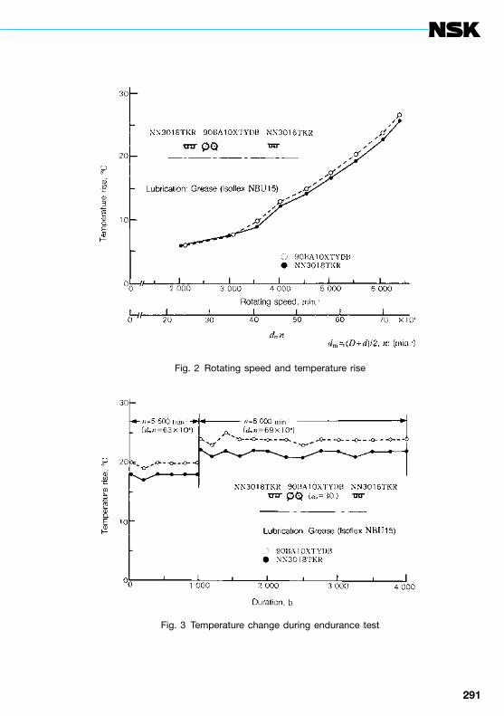
290 291

Fig. 2　Rotating speed and temperature rise

Fig. 3　Temperature change during endurance test

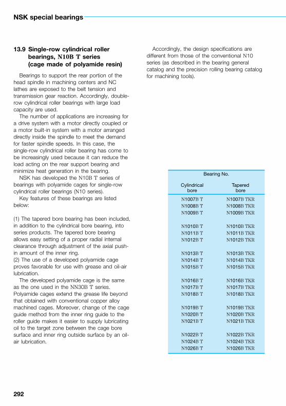
292


13.9 Single-row cylindrical roller bearings, N10B T series (cage made of polyamide resin)

Bearings to support the rear portion of the head spindle in machining centers and NC lathes are exposed to the belt tension and transmission gear reaction. Accordingly, double-row cylindrical roller bearings with large load capacity are used.

The number of applications are increasing for a drive system with a motor directly coupled or a motor built-in system with a motor arranged directly inside the spindle to meet the demand for faster spindle speeds. In this case, the single-row cylindrical roller bearing has come to be increasingly used because it can reduce the load acting on the rear support bearing and minimize heat generation in the bearing.

NSK has developed the N10B T series of bearings with polyamide cages for single-row cylindrical roller bearings (N10 series).

Key features of these bearings are listed below:

(1) The tapered bore bearing has been included, in addition to the cylindrical bore bearing, into series products. The tapered bore bearing allows easy setting of a proper radial internal clearance through adjustment of the axial push-in amount of the inner ring.(2) The use of a developed polyamide cage proves favorable for use with grease and oil-air lubrication.

The developed polyamide cage is the same as the one used in the NN30B T series. Polyamide cages extend the grease life beyond that obtained with conventional copper alloy machined cages. Moreover, change of the cage guide method from the inner ring guide to the roller guide makes it easier to supply lubricating oil to the target zone between the cage bore surface and inner ring outside surface by an oil-air lubrication.

Accordingly, the design specifications are different from those of the conventional N10 series (as described in the bearing general catalog and the precision rolling bearing catalog for machining tools).

Bearing No.

Cylindricalbore

Taperedbore

N1007B TN1008B TN1009B T

N1010B TN1011B TN1012B T

N1013B TN1014B TN1015B T

N1016B TN1017B TN1018B T

N1019B TN1020B TN1021B T

N1022B TN1024B TN1026B T

N1007B TKRN1008B TKRN1009B TKR






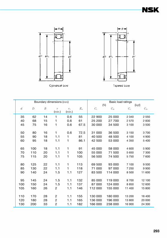
292 293

Boundary dimensions (mm) Basic load ratings(N) {kgf}

d D B r(min.)

r1

(min.)Ew Cr C0r Cr C0r

35 40 45

50 55 60

65 70 75

80 85 90

95100105

110120130

62 68 75

80 90 95

100110115

125130140

145150160

170180200

141516

161818

182020

222224

242426

282833

111

11.11.1

1.11.11.1

1.11.11.5

1.51.52

222

0.60.60.6

0.611

111

111.1

1.11.11.1

1.11.11.1

556167.5

72.58186.1

91100105

113118127

132137146

155165182

22 900 25 200 30 000

31 000 40 500 42 500

45 000 55 000 56 500

69 500 71 000 83 500

85 000 87 000112 000

130 000136 000166 000

25 000 27 700 34 500

36 500 48 500 53 000

58 000 71 500 74 500

93 000 97 000114 000

119 000124 000155 000

180 000196 000238 000

2 340 2 570 3 100

3 150 4 100 4 350

4 600 5 650 5 750

7 100 7 250 8 500

8 700 8 85011 400

13 20013 80016 900

2 550 2 830 3 500

3 700 4 900 5 400

5 900 7 300 7 600

9 500 9 90011 600

12 10012 60015 800

18 40020 00024 300

294


13.10 Sealed clean bearings for rolling mill roll neck

A large quantity of roll cooling water (or rolling oil) or scales is splasthed around the roll neck bearing of the rolling mill. Moreover, the roll and chock must be removed and installed quickly. In this environment, the oil seal provided on the chock may be readily damaged and the roll neck bearing may be exposed to entry of cooling water or scale.

Upon investigation, used grease from the bearing was found to be high in water content. Also, the bearing raceway often shows numerous dents due to inclusion of foreign matter, indicating progress of fatigue on the raceway surface.

The roll neck sealed clean bearing, which NSK has developed on the basis of the above investigation and analytical results, is already employed in large quantity inside and outside of Japan.Features of the roll neck sealed clean bearing are listed below:

(1) Reduce the frequency of grease replenishment. The conventional man-hour needed for grease supply each day per bearing becomes totally unnecessary. In this way, maintenance costs can be reduced substantially.(2) Seals are incorporated on both ends of the bearing, thus eliminating the possibility of damaging a seal during handling and effectively preventing entry of water and scale into the bearing. As a result, the rolling fatigue life can be improved substantially and there are fewer accidental seizures.(3) The grease consumption can be reduced. For example, when assuming a case of three turns of chock for the cold rolling mill work rolls of five stands, the total number of bearings becomes 60 (4 ´ 5 stands ´ 3 turns) and, in this case, 10 to 15 tons of grease can be saved annually.

(4) The cleaning interval of a bearing can be extended. Conventional interval of partial cleaning every three months or so can be extended to every six months or more, thereby reducing the amount of maintenance work. However, the optimum interval needs to be determined after considering and experimenting with the particular conditions of the specific rolling mill.(5) Reduction of the grease supply man-hour and of the grease consumption can decrease the contamination around a roll mill and roll shop and thus improves the cleanliness of the work environment.

Fig. 1 shows a typical assembly of a sealed clean bearing for the roll neck. Table 1 shows typical dimensions of a representative sealed clean bearing. For details, refer to the NSK catalog “Large-Size Rolling Bearings”, CAT. No. E125.

294 295

Fig. 1　Typical assembly of sealed clean bearing for roll neck

Table 1 Boundary dimensions of a sealed clean bearing for a roll neck

Bearing No.Boundary dimensions (mm)

d D B4 C4

STF 343 KVS 4551 Eg

STF 457 KVS 5951 Eg

STF 482 KVS 6151 Eg

343.052

457.200

482.600

457.098

596.900

615.950

254.000

276.225

330.200

254.000

279.400

330.200

296


13.11 Bearings for chain conveyors

Many chain conveyors are used to transport semi-finished products and finished products (coil, etc.) between processes in a steelmaking plant. Bearings dedicated to these chain conveyors are used. The inner ring is fixed to the pin connecting the link plates while the outer ring functions as a wheel to carry the load on the rail by rolling.

Though varying in design depending on the purpose, typical conveyors used in steelmaking plant are shown in Figs. 1 and 2.

The bearing for chain conveyors rotates with outer rings at extremely low speed while being exposed to relatively heavy load and shock load. They are also used in poor environments with lots of water and scale at high temperature. In view of enhancing the breakdown strength by providing the roller (outer ring) with high wear resistance, a thick-wall design is employed and carburization or special heat treatment is made to increase the shock resistance. A full-complement type cylindrical roller bearing is designed to sustain these heavy loads. A double-row cylindrical roller bearing is not needed usually.

Either the S type (side seal type, Fig. 3) or labyrinth type (Figs. 4 and 5) is available. Thus, dust-proof and water-resistance as well as grease sealing are ensured. In particular, the S type has achieved further improvements in seal effectiveness through the use of a contact seal.

Normally, the outer ring outside has a cylindrical surface. There are various types: some with the outer ring width longer than the inner ring width (Figs. 3 and 4) and some with the outer ring and inner ring widths nearly equal (Fig. 5). Features of the chain conveyor bearing may be summarized as follows:

(1) The rollers (outer rings) are thick and made resistant to shock load and wear through carburization or special heat treatment.(2) Special tempering allows use at high temperature.(3) Optimum grease is filled for maintenance free operation, ensuring superior durability and economic feasibility.

(4) The seal construction is superior in grease sealing and dust- and water-proof, with a measure incorporated to prevent dislodgement of the seal by shock. In particular, the S type, which uses a contact seal, can realize improved sealing. The benefits of improved sealing include extension of the bearing life, substantial reduction of both supply grease and supply man-hours, and even cleaner surroundings.

Typical specifications on this bearing are shown in Table 1. Please contact NSK for information on bearings not shown in Table 1.

296 297

Fig. 1

Fig. 2

Fig. 3

Fig. 4 Fig. 5

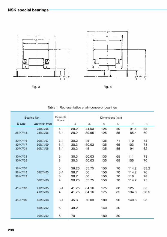
298


Table 1 Representative chain conveyor bearings

Example figure

Bearing No. Dimensions (mm)

S-type Labyrinth type d d1 D C B B1

　28RCV13

30RCV1630RCV1730RCV21

30RCV2330RCV25


　

41RCV07　

45RCV09

　

　

28RCV0528RCV06


　　

　38RCV05

　38RCV06

41RCV0541RCV06

45RCV06

48RCV02

70RCV02

43,4

3,43,43,4

33

33,434

3,44

3,4

5

5

28.228.2

30.230.330.2

30.330.3

38.2538.738.738.25

41.7541.75

45.3

48.2

70

44.0339.95

4550.0345

50.0350.03

55.75565655.75

64.1664.16

70.03

　

　

125125

135135135

135135

150150150150

175175

180

140

180

5055

716555

6565

70707070

8085

90

50

80

91.485.4

110103

94

111105

114.2114.2116114.2

125134.8

140.6

　

　

6560

787862

7870

83.2767875

8590.5

95

　

　

Fig. 3 Fig. 4

298 299

Basic load ratingsS-type Labyrinth type

(N) {kgf} (N) {kgf}Cr C0r Cr C0r Cr C0r Cr C0r

　160 000

275 000253 000196 000

253 000242 000

294 000294 000294 000

　

380 000　

435 000

　

　

　177 000

330 000298 000215 000

298 000282 000

350 000350 000350 000

　

485 000　

590 000

　

　

　16 400

28 00025 80020 000

25 80024 700

30 00030 00030 000

　

39 000　

44 500

　

　

　18 100

34 00030 50022 000

30 50028 700

35 50035 50035 500

　

49 500　

60 000

　

　

198 000175 000

285 000253 000196 000

　　

　305 000

　305 000

380 000415 000

485 000

229 000

380 000

233 000198 000

350 000298 000215 000

　　

　365 000

　365 000

485 000540 000

690 000

278 000

675 000

20 20017 800

29 10025 80020 000

　　

　31 000

　31 000

39 00042 000

49 500

23 400

39 000

23 80020 200

35 50030 50022 000

　　

　37 500

　37 500

49 50055 000

70 500

28 400

69 000

Fig. 5

300


13.12 RCC bearings for railway rolling stock

Recent trains as well as the rolling stock are required to be high speeds and maintenance-free to satisfy the technical trends and environments.

Among the railway rolling stock, the axlebox bearings which run under the severe conditions such as large vibration and strong shocks when passing the rail joints or points, harsh environments with dust, rain and snow, are required to be high reliability for a long time.

NSK developed RCC bearings (Sealed cylindrical roller bearings for railway axle) to meet the above requirements. The RCC (Rotating end Cap type Cylindrical roller bearing) is a sealed bearing unit in which specially designed oil seals are attached directly to both ends of a double-row cylindrical roller bearing with double collars and filled with a dedicated long-life grease. (Fig. 1) The exclusive greases are the greases which are popularly used at AAR (Association of American Railroads) or long-life grease for axlebox developed by NSK.

The RCC bearings have the following features.1. Unit construction, enabling easy handling.2. The axle end can be exposed simply by

removing an end cap, facilitating flaw detection of the axles or grinding of axles.

3. The roller and cage sub-unit can be removed from inner and outer rings during disassembly, making cleaning and inspection easier.

4. This unit bearing has an anti-rusting coating applied over the outer ring outside. An adaptor to be set on the outer ring is enough for a bearing box, thereby making the construction around the bearing simpler and reducing the weight.

Now, due to the good results, RCC bearings are widely used in new electric and passenger cars of both private and semi-national (JR) railways in Japan. Specifications of principal NSK RCC bearing units are shown in Table 1.

Unit No.d

J-801 130

J-803 120

J-805 120

J-806 120

J-807 130

J-810A 120

J-811 120

J-814 130

J-816 130

J-817 120

J-818 90

J-819 120

J-820 85

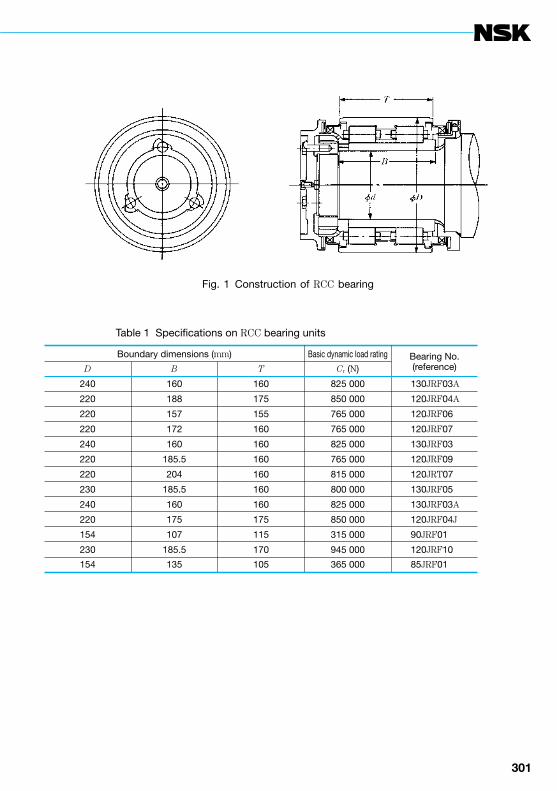
300 301

Table 1 Specifications on RCC bearing units

Boundary dimensions (mm) Basic dynamic load rating Bearing No.(reference)D B T Cr (N)

240 160 160 825 000 130JRF03A

220 188 175 850 000 120JRF04A

220 157 155 765 000 120JRF06

220 172 160 765 000 120JRF07

240 160 160 825 000 130JRF03

220 185.5 160 765 000 120JRF09

220 204 160 815 000 120JRT07

230 185.5 160 800 000 130JRF05

240 160 160 825 000 130JRF03A

220 175 175 850 000 120JRF04J

154 107 115 315 000 90JRF01

230 185.5 170 945 000 120JRF10

154 135 105 365 000 85JRF01

Fig. 1　Construction of RCC bearing

Every care has been taken to ensure the infor mation in this publication is accurate but no liability can be accepted for any errors or omissions. © Copyright NSK 2011. The contents of this publication are the copyright of the publishers. Printed in Japan. Ref: TR/A/E/02.14 - E728e

NSK Sales Offices – Europe, Middle East and Africa

Please also visit our website: www.nskeurope.com | Global NSK: www.nsk.com

UKNSK UK Ltd. Northern Road, Newark Nottinghamshire NG24 2JFTel. +44 (0) 1636 605123 Fax +44 (0) 1636 [email protected]

France & BeneluxNSK France S.A.S. Quartier de l’Europe 2, rue Georges Guynemer 78283 Guyancourt Cedex Tel. +33 (0) 1 30573939 Fax +33 (0) 1 30570001 [email protected]

Germany, Austria, Switzerland, NordicNSK Deutschland GmbH Harkortstraße 15 40880 Ratingen Tel. +49 (0) 2102 4810 Fax +49 (0) 2102 4812290 [email protected]

ItalyNSK Italia S.p.A.Via Garibaldi, 21520024 Garbagnate Milanese (MI)Tel. +39 02 995 191Fax +39 02 990 25 [email protected]

Middle EastNSK Bearings Gulf Trading Co. JAFZA View 19, Floor 24 Office 2/3Jebel Ali Downtown, PO Box 262163Dubai, UAE Tel. +971 (0) 4 804 8205Fax +971 (0) 4 884 7227 [email protected]

Poland & CEENSK Polska Sp. z o.o. Warsaw Branch Ul. Migdałowa 4/73 02-796 Warszawa Tel. +48 22 645 15 25 Fax +48 22 645 15 29 [email protected]

RussiaNSK Polska Sp. z o.o. Russian Branch Office I 703, Bldg 29, 18th Line of Vasilievskiy Ostrov, Saint-Petersburg, 199178Tel. +7 812 3325071 Fax +7 812 3325072 [email protected]

South AfricaNSK South Africa (Pty) Ltd.25 Galaxy Avenue Linbro Business ParkSandton 2146 Tel. +27 (011) 458 3600Fax +27 (011) 458 [email protected]

SpainNSK Spain, S.A. C/ Tarragona, 161 Cuerpo Bajo 2a Planta, 08014 Barcelona Tel. +34 93 2892763 Fax +34 93 4335776 [email protected]

TurkeyNSK Rulmanları Orta Doğu Tic. Ltd. Şti 19 Mayıs Mah. Atatürk Cad.Ulya Engin İş Merkezi No: 68/3 Kat. 6 P.K.: 34736 - Kozyatağı - İstanbul Tel. +90 216 4777111 Fax +90 216 4777174 [email protected]

http://www.nskeurope.com

http://www.nsk.com

technical report - nsk-literature.com

Documents