technical report standard title pace 1 · pdf filetechnical report standard title pace 2....
TRANSCRIPT

TECHNICAL REPORT STANDARD TITLE PACE
2. Go"elnmen' "ce ... ion No. 3. RocipiO/ll'1 Catolo. No.
- FHWA/TX-84;/03 +340-1 ~~~ __ ~~~ ____________ ~ __________________ ' ______ ~~ __ ~ _______________ 4 __ 1 -
4. T"I. and Subli.le 5. R.,.rt Ooto _
April 1983 Pressuremeter Design of Shallow Foundations 6. PorI.,.",,,, O'teI'll.trOft C.,..
7. "u'horl II
Jean-Louis Briaud and Gerald Jordan 9. P.,lo,ming Orgonl zalron Nome and Addr ...
Texas Transportation Institute The Texas A&M University System College Station, Texas 77843
12. Spon.o,ing "goncy Nomo and Add, ... ------------------------~
8. It.''O'''''''1I O, •• n' .otion ROllo,t No.
Research Report 340-1 10. Work Unit No.
II. Conl,oct or G,an' No.
Research Study 2-5-83-340 13. Typ. of Rapo,t onll P.riod Co ... r.cI
State Department of Highways and Public Transportatio I t 'm September 1982 n erl - April 1983
Transportation Planning Division P. O. Box 5051 Austin, Texas 78763
14. Sttonlorin, ..... ncy C040
--------~--------.------------------~------------------------~ 1 S. Supplementary Not .. Research performed in cooperation with DOT, FHWA. Research Study Title: The Pressuremeter and the Design of Highway Related
Foundations. 16_ "ba"oct
In this report, a detailed description is made of the established procedures to design shallow foundations on the basis of preboring pressuremeter tests. Both the bearing capacity and settlement calculations are outlined in the form of step-by-step procedures. Design examples are given and solved. An indication of the precision of the methods is presented by comparing the predicted behavior to the measured behavior for over 50 case histories.
17. Key Wo,d,
Shallow Foundation, Pressuremeter Design, Clay, Sand, Rock
II, OlatrlllutlOft St •• _ont
No restriction. This document is available to the public through the National Technical Information Service, 5285 Port RO'yal Road, Springfield, Virginia 22161.
19 Se.,uri t)l ClolSi I. (01 thi. report) 20. S.curlty Cl ... II. f.f thta , ... 1 21. No. 01 p.... 22. Price
I
J
~~ __ cl~a~s_s~if~l='e~d~ ___________ ~~ __ u_n_c_la~s_s_i_f_i_ed ____________ ~ __ 7_9 ____ ~ __________ ~1 Form DOT F 1700.7 CI.UI

PRESSUREMETER DESIGN OF SHALLOW FOUNDATIONS
by
Jean-Louis Briaud and Gerald Jordan
Research Report 340-1
The Pressuremeter and the Design of Highway Related Foundations Research Study 2-5-83-340
Sponsored by
State Department of Highways and Public Transportation In cooperation with the
U. S. Department of Transportation, Federal Highway Administration
Texas Transportation Institute The Texas A&M University System
College Station, Texas
April 1983

SUMMARY
In this report, a detailed description is made of the established
procedures to design shallow foundations on the basis of preboring
pressuremeter tests. Both the bearing capacity and settlement calcu-
lations are presented in the form of step-by-step design procedures.
The bearing capacity equation is:
q = kp * + q P . Le 0
where q is the bearing capacity of the foundation, k is the pressurep
meter bearing capacity factor, PL~ is the equivalent net limit pressure
obtained from preboring pressuremeter tests performed within the zone
of influence of the foundation and qQ is the vertical total pressure at
the foundation level prior to construction. The bearing capacity factor
k depends on the relative depth of embedment of the foundation, the type
of soil, and the shape of the foundation. Charts for k have been pro
posed by Menard and Gambin in 1963, Baquelin, Jezequel and Shields in
1978, and Bustamante and Gianeselli in 1982.
The three charts are presented and used to solve several example
problems. The results of those examples show that generally the Busta
mante-Gianeselli method gives the lowest bearing capacity-values, that
the Menard-Gambin method gives higher values and that the Baquelin-Jeze
quel-Shields method gives values which are slightly higher than the
values obtained with the Menard-Gambin method.
The settlement equation is:
2 10.. - 0.. 1 S ="9 E q. Bo' (Ad ~) + 9" E q Ac B
d . B c o
iii

where S is the settlement of the foundation, Ed is the average modulus
obtained from preboring pressuremeter tests performed within several
foundation widths below the foundation level, q is the net bearing pres
sure, Bo is a reference width, B is the width of the foundation, Ad and
AC are 'shap~ factors, a is a rheologic factor, Ec is the average modulus
obtained from preboring pressuremeter tests performed immediately below
the foundation level.
The two terms of the settlement equations correspond to two dis
tinct components: the settlement due to shearing stresses (deviatoric
component) and the settlement due to hydrostatic compression {spherical
component). When the width of the foundation is small compared to the
thickness of the bearing stratum (common case of shallow foundation),
the settlement due to shearing stresses is larger than the settlement
due to the hydr?static compression.
The above settJement equation applies when the ratio of the
foundation width to the thickness of the bearing stratum is small. This
equation is modified when the ratio is large and in this case the
pressuremeter settlement analysis should be complemented by a consoli
dation test analysis. Example of settlement calculations are presented
to illustrate the design procedures in various cases.
The above bearing capacity and settlement rules are evaluated ?y
presenting the results of comparisons between predicted andmeasured.
behavior for over 50 case histories. It must be emphasized that one
of the critical elements in the accuracy of the predictions is the
performance of quality pressuremeter tests by trained
professionals.
, iv

IMPLEMENTATION SETTLEMENT
. _ •. o-~ •• -~_ ~
This report gives the details of existing pressuremeter methods
for the design of shallow foundations. These methods require the use
of a new piece of equipment: a preboring pressuremeter. These methods
are directly applicable to design practice and should be used in
parallel with current methods for a period of time until a final de
cision can be made as to their implementation.
v
:"., ,

ACKNOWLEDGMENTS
The authors are grateful for the continued support and encourage
ment of Mr. George Odom of the Texas State Department of Highways and
Public Transportation.
DISCLAIMER
The contents of this report reflect the views of the authors who . are responsible for the opinions, findings, and conclusions presented herein. The contents do not necessarily reflect the official views or policies of the Federal Highway Administration, or the State Department of Highways and Public Transportation. This report does not constitute a standard, a specification, or a regulation.
vi
.. "
. -.:" .

TABLE OF·CONTENTS
PRESSUREMETER DESIGN OF SHALLOW FOUNDATIONS
SUMMARY . . . . . . . . . . ~ .
GLOSSARY OF TERMS AND EQUATIONS
1. INTRODUCTION...
2. BEARING CAPACITY
2.1 Theoretical Background
2.2 Methods for Finding the Bearing Capac~ty Factor, K
2.3 Bearing Capacity Equation .......... .
* 2.4 Calculating PLe' the Equivalent Limit Pressure
2.5 Calculating He, the Equivalent Depth of Embedment ..
2.6 Obtaining k, the Pressuremeter Bearing Capacity Factor . . . . . . . . . . . . . . . . . . . . .
2.7 Calculating qp' qsafe' and qnet ....... .
2.8 Reduction of the Bearing Capacity Factor for· Footings Near Excavations .
3. SETTLEMENT.. . .
3.1 Menard Method.
3.1.1 Theoretical Background.
Page
iii
x
1
2
2
2
12 12
12
13
13
14.
16
16
16
3.1.2 Calculating the Layer Moduli 18
3.1.3 Calculating Ec and Ed 21
3.1.4 Obtaining a and A • . • 22
·3.1.5 Calculating the Settlement 22
3.1.6 Special Case of a Thin Soft Layer at Depth 22
3.1.7 Special Case of a Thin Soft Layer Close to the Ground Surface . . . . . . . . . . . . . . 23
vii
......

Page
3.2 Settlement + Schmertmann Method Using Pressuremeter Moduli ........ .
4. EXAMPLES OF DESIGK PROBLEMS AND THEIR SOLUTIONS
25
28
5.
Example la Shallow Footing on a Clay (Menard Method) 30
Example lb Shallow Footing on a Clay (B.J.S. Method) . 32
Example lc Shallow Footing on a Clay (B.G. Method) . 34
Example 2a Shallow Footing on Sand (Menard Method) . 37
Example 2b Shallow Footing on Sand (B.J.S. Method) 39
Example 2c Shallow Footing on Sand (B.G. Method) 41
Example 3 Strip Footing on Sand.
Example 4
Example 5
Example 6
Rectangular Footing on a Layered Soil (Menard Method) . . . . . . . . . . .
Strip Footing on a Soft Layer at Depth ..
Mat Foundation on a Soft Layer . . . .
COMPARISON BETWEEN ·PREDICTED AND MEASURED BEHAVIOR . . . . REFERENCES .......... -.......... .
viii
.... ~. .
44
50
54
57
59
65
.~ -.

Figure
1
2
3
4
5
6
7
8
9
10
11
12
13
14
15
16
17
LIST OF FIGURES
Pressuremeter Bearing Capacity Method for Foundations .............. .
Footing Capacity Due to lateral Soil Support
Bearing Capacity. Factors for Menard ..... .
Beari ng: apacity Factors for Baquel in, Jezeguel, Shields Method ................ .
Beari ng Capacity· Factors for Bustamante and Giansell i
Soil Categories for Use with Menard Bearing Capacity Chart of Figure 3 .................. .
Soil Categories for Use with Bustamante and Gianselli Bearing Capacity Chart of Figure 5 .....•..
Reduction of the Bearing Capacity of a Footing as a Function of Tan S . . . ...
Rheological Factor, a
Shape Factors Ac' Ad ......... .
layers to be Considered in the Settlement Analysis
Schmertmann Settlement Concepts and Influence Factor Distribution ...... .
Pressuremeter Settlement Concepts ..
Predicted Versus Measured Settlement (Very Small Settlement) ...... .
Predicted Versus Meansured Settlement (Moderate Settlement) ......•.
Predicted Versus Measured Settlement (large Settlement) ........ .
. . . . . . ..
Comparison of the Bearing Capacity Factors Predicted by the B.G. Method and Measured by Menard ..•....
ix
3
4
6
7
9
10
11
15
19
19
20
27
60
61
62
63
64

GLOSSARY OF TERMS AND EQUATIONS
BEARING CAPACITY
k = Pressuremeter bearing capacity factor p (sphere) L
= -p"'---r( c-y""'l~i n-d'-e-r) L
* PL = net limit pressure = PL - Poh
POH = total horizontal stress in soil at rest
PL = ultimate limit pressure
qp = pressuremeter bearing capacity
* qp = k PLe + qo
qsafe = k P~e/3 + qo
* where PLe = equivalent net limit pressure
qo = total stress overburden at foundation level
He = equivalent depth of embedment
* n PI . He = ~ t.Z i
_1 -*-
1 PLe
q" = reduced bearing capacity for slopes and excavations p
qp = ~ qp where: ~ = reduction factor
qp = normal bearing capacity
x

..
~ i . 'J." 'f·. ••••• ..o; ...... ~ •• ". -.'" • ... ~~ ..
Qv = vertical load on the foundation
f = friction on the side of the foundation 5
C = undrained soil shear strength u .
..~ .. " : ..... -'.", ; >.' .... : ...
D = actual depth of embedment of the foundation
L = length of the foundation
B = width of the foundation
xi

SETTLEMENT
ST = long-term, drained settlement
Su = rapid, undrained settlement
Sc = consolidation settlement = sT - Su
Layer moduli by harmonic mean:
n
n = L __ 1 __ where Ek = average PMT modulus within kth layer Ek 1 Ei
E. = moduli from PMT results in kth layer 1
Settlement with a thin, soft layer at depth:
s = s· + Sll
s· = settlement without considering soft layer
Sll = settlement of soft layer alone
= ( 1 (l Esoft
where ~crv = change in vertical pressure between top
and bottom of soft layer
H = thickness of soft layer
(l = rheological factor
E = pressuremeter modulus
Settlement of a thin, soft layer at ground surface: n L (li Pi
S = ~Z. 1 E. 1 1
i = layer number,
where S = coefficient based on the safety factor, F
xii
.. ". ~. .

F = ultimate bearing pressure actual bearing pressure 2 F e = "3 (F-f)
~vi = change in vertical pressure in the ith layer
ai = rheological factor of each layer
~zi = thickness of each layer
The pressuremeter settlement equation:
S = total footing settlement
Ed = pressuremeter modulus within zone of deviatoric
tensor influence
_1_ = 1 (L +. 1 + _1_ + 1 + 1 ) Ed 4 E1 0.85E2 E3/6 2.5E6/ 8 2.5E9/ 16
E. = pressuremeter modulus within zone of spherical tensor 1
influence
E = first layer average modulus c q = net footing bearing pressure (qnet)
Bo = reference width = 2 ft or 60 cm
Ad = devia~oric shape factor .. '
A = spherical shape factor' c
a = rheological factor
STRESS, STRAIN, MODULI
o = total stress tensor
= 0 + 0 s d
where: Os = spherical stress component
xiii

ad = deviatoric stress component
likewise: ~ = spherical strain component 's
Ed = deviatoric strain component
E = Young's Modulus
y = Poisson's Ratio
G = Shear Modulus
K =.Bulk Modulus
xiv

CHAPTER 1. - INTRODUCTION
The established procedures to design shallow foundations on the
basis of preboring pressuremeter tests are presented in detail in this
report. In a first part the bearing capacity and settlement calculations
are described in the form of step-by-step procedures. Then the accuracy
of the methods presented are evaluated by comparing predicted and mea
sured behavior of shallow foundations for over 50 case histories. Fin
ally, design examples are solved to illustrate the design rules.
It must be emphasized that one of the critical elements for the
successful prediction of shallow foundation behavior using these design
rules is the performance of quality pressuremeter tests. Such quality
pressuremeter tests can only be performed by trained professionals.
1

CHAPTER 2. - BEARING CAPACITY
2.1 Theoretical Background
Figures 1 and 2 show the analogy between the pressuremeter limit
pre.ssure PL and the ul timate bearing capacity qp' If the penetration
of a circular footing is associated with the expansion of a spherical
cavity, then the ultimate bearing capacity of that footing is given by
the limit pressure to the expansion of a spherical cavity (PL sphere).
The pressuremeter test on the other hand is associated with the ex
pansion of a cylindrical cavity and leads to a limit pressure (PLCy
linder). The ratio between the pressuremeter limit pressure and the
ultimate bearing capacity of a circular footing could therefore be
expressed as the pressuremeter bearing capacity factor, k:
PL (sphere) k =-----
PL(cylinder) (1) .
This theoretical bearing capacity factor can be evaluated using plastic
ity theory; such values of k vary from 1.4 to 2.4 (6). However, the k
values have been determined from full scale field tests.
2.2 Methods for Funding the Bearinq Capacity Factor, k
At present there are three methods available to find the bearing
capacity factor for shallow foundations. These are: the Menard chart
2

f = ap* S L
• p . L
Theoretically k = I. 4 To 2.4
However k And a Obtained
From Load Test Data
FIGURE 1: Pressuremeter Bearing Capaci.ty. Method forFou~dattons
3
. ,

Soi I
6c . u
I I III , I
Soil
1/11/111111 111/111.11/11111111/1//111/1111
Bearing Capacity Of Plate = 6 Cu Part Of Bearing Capacity Due To Vertical Resistance Only = 2cu Part Of Bearing Capacity Due To Latera I Resistance Only = 4cu Where Cu :. Undrained Shear Strength
• • q = k PLe
6c u = kx 4cu --~ ... -k=1.5
FIGURE 2: Footing Capacity Due To Lateral Soil Support
4

(Ref. 10, Fig. 3), charts by Baguelin, Jezeguel, and Shields (B.J.S., Ref.
1, Fig. 4), and a chart developed after Bustamante and Gianselli (B.G.,
Ref. 3, Fi g. 5).
Figure 5 was obtained from the early part of the B.G. chart for
piles. It wa_s assumed that circular footings have the same capacity
factors as very shallow bored piles. This led to the design curves for
circular footings. The curves for the strip footings were obtained by
reducing consistently the k values of the circular footings.
The Menard, the B.J.S., and the B.G. charts relate the bearing
capacity factor to -a relavtive depth for various soil classifications.
These charts can hand1~ circular, square, and strip footinqs. Values of
k must be interpolated for rectangular footings.
The Menard and B.G. charts use similar soil classification tables
to distinguish between design curves (Figures 6 and 7). Both charts
express k as a function of the ratio of the equivalent embedment depth
of the foundation (He) to the radius of the foundation R. For non cir~
cular footings the radius of the foundation is considered to be half
the width B of the foundation.
The B.J.S. charts express k as a function of the depth to width
ratio He {Figure 4}. There are four charts; each one is used for a B
single soil classification and gives different curves for different soil
* strengths (p ). This seems to allow for a more detailed determination L
of k. Anytime an interpolation is necessary to find the bearing capa-
city factor, a linear variation is assumed to exist between the design
points on the chart; for rectangular footings the interpolation para
meter is ~ where L is the length of the foundation.
5
- --------- --~~---.:....~~~~~~~~~~~~~~~

k
3~----~------~-----+------4---~~----~
.Yo
.. S-o +> U to u.. 2 ~ .... U to 0... to
U
en t:
co,eoof1 1.
co,eQOf1111.~ t-__ ~~~---+-II!::.---___ -=i~==---+--::::ao"-~co'eQor'll1L ....
S-'to
QJ co
0.8 o 2
Equivalent Depth of Embedment He Radius of Foundation ' if
teoOrY'II cot8Q;ryl
3
FIr,UP.E 3: Bearing Capacity Factors Fo .. Menard (Reference 10)
--_ ..
CIRCULAR OR SQUARE FOOT I NG
2R = I L
STRIP FOOTING
2R =0 L
He R

.. So
+..l u n:s
LL.
.,.... u n:s 0.. n:s u en c .,.... S-
I 83,540
3~--+---+---~~~---4----~--+--
ROUND
83,540= pi
--2 I-----I-F-+--t-
. ,.... u n:s 0.. n:s u en c .,.... S-
~--f62,660
3r---+---+---1-~~---+--~
ROUND ~-- 20,880 = pi
I ._--t-10,440
_ 62,660 -2r---~~4---~--~~~~--+----__ 20,880-
I p. 10440- .. , I
STRIP
~ 0.8 ~ 0.8 c:a SILT c:a
o
CLAY
(pI in pst)
1234567 Equivalent D~pth of Embedment He
Width of Foundation ' 11
(pi in pst) o~~~~~~~~~~~~~~
o 123 4 5 6 Equivalent D~p~n of Embedment He
Width of ~Foundation ' B
FIGURE 4: Bearing Capacity Factors For Baguelin, Jezeguel, Shields Method (Reference 1) .

8
.. ~ " 7
'" S-o +J 6 u ttl
LL. 5
~ .,... u 4 ttl 0-ttl
U 3 " .
Ol 00 s:: .,... 2 s-
ttl Q)
I al ,0.8
SAND AND GRAVEL I
V 125,300 l--
V p
V ROUND V I....- f-4I,770' f.-
or 1/ L..-V SQUARE
V-V ./
." 20,890 - -- -125,300 t
j V / ---L,..- _41770
t V 10.:140- - .... - STRIP
~ /-
~ r,/ - -J-- - 8,350
",.-I-
(p; In pst)
° , I I ,
° 2 3 4 5 .6 7 8 9 10 II 12 13
Equivalent Depth of Embedment He Width of Foundation ' 13
FIGURE 4: (Continued)
~ .. s-o +J U ttl
LL.
~ .,... U ttl 0-ttl
U
Ol s:: .,... s-ttl Q) al
5
4
3
2
I I ROCK
pt.
(pi In pst)
012345678
Equivalent Depth of Embedment He Width of Foundation ' If
'"

. k for Shallow Foundations
3~----~----~------~----~------+---__ ~
--- Circular or Square - - Strip
~ 2~-----+--~---+----~-+-------r------~-------
.,....
-- -- -- - --
CAT. I
O~~--~~--~--~~--~--~~--~--~~ .. o 2 ,4
Equivalent Depth of Embedment He Radi us of Foundation' R
5
FIGURE 5: Bearing Capacity Factors For Bustamante and Gianeselli (Reference 3)
9
. -.'-.'
He R

, ~
LIMIT PRESSURE
(psf)
o - 25000
o - 15000
37500 - 84000
25000 - 63000
8000 - 17000
21000 - 63000
21000 - 42000
83500 - 209000
62500 - 125000
Clay
Si It
SOIL TYPE
Firm Clay or Marl
Compact Sil t
Compressible Sand
Soft or Weathered Rock
Sand and Gravel
Rock
Very Compact Sand and Gravel
CATEGORY
I
II
III
lIlA
Fiqure 6: Soil Categories for Use with Menard Bearing Capacity Chart of Figure 3 (Reference 10)
10

LIMIT PRESSURE
21
25
(psf)
15000
17000
15000
- 42,000
- 63,000
31 - 84,000
21 - 52,000
52 - 84,000
63,000
94,000
52,000
94,000
SOIL TYPE CATEGORY
Soft Clay
Silt and Soft Chalk 1
Loose Clayey, Silty, or Muddy Soil
Medium Dense Sand and Gravel
Clay and Compact Silt
Marl and Limestone-Marl
Weathered Chalk 2
Weathered Rock
Fragmented Chalk
Very Compact Marl
Dense to Very Dense Sand and Gravel 3
Fragmented Rock
Figure 7. Soil Categories for Use with Bustamante and Gianeselli Bearing Capacity Chart of Figure 5 (Reference 3)
11

The B.J.S. and Menard charts give similar k values; the B.G. chart
gives consistently lower values. The effects of these differences on
bearing capacity can be seen in examples 1a,b,c and 2a,b,c.
2.3 Bearing Capacity Equation
The ultimate bearing capacity, qp is:
. (2).
where
k = pressuremeter bearing capacity factor (Figs. 3, 4, 5),
* PL = net limit pressure = PL - Poh'
Poh = total horizontal stress at rest PL = limit pressure (from test),
pte = equivalent net limit pressure near the foundation level, and
q = total stress overburden pressure at foundation level. u
* 2.4 Calculating PLe ' the Equivalent Limit Pressure
* * * PL1 x PL2 x • • . x PLn (3).
where PL1' ... , PLn are the net limit pressures obtained from tests
performed within the (+) 1.SB to (-) 1.SB zone near the foundation level.
See examples 3 and 4.
2.5 Calculating He' the Egui'va 1 ent Depth of Embedment
n * H = L 6z. PLi e 1 1 -r PLe
(4) .
12

* where PLi are the limit pressures obtained from tests between the ground
surface and the foundation level, and ~zi are the thicknesses of the ele
mentary layers corresponding to the pressuremeter tests. See examples
3 and 4.
2.6 Obtaining k, the Pressuremeter Bearing Capacity Factor
The relative embedment depih is H IR for the Men~rd and the B.G. e
method, and HelB for the B.J.S. method. The parameter R is the radius
of the footing or half the width and B is the diamet~r or the width of
the footing.
The soil category is determined from Figures 6 and 7 for Menard
and B.G. method, respectively; B.J.S. has separate charts for different
soils. Then the bearing capacity factor is read on Figure 3, 4, or 5.
If the footing .is rectangular, linear interpolation is performed between
the case of a square footing and the case of a strip footing; the inter
polating parameter is S/L. See Examples 1, 2, and 3.
2.7 Calculating qp~qsafe' and qnet
+ q , o
* q - q - kPLe net - qsafe - 0 - --
3
See Examples 1, 2, and 3, Section 3.
.. : .....
(5) .
(6) .
(7) .
13

~ Reducti on of . th~._~_~~.~.i.!l.g .. ~a.p~'£~!l'_~~<:.!or_.!.Q!'. y'~oti ngs Nea r
Excavations
It is sometimes necessary or practical to set footings near slopes
or excavations. In this case the bearing capacity factor must be re
duced to allow for the reduced lateral confinement in the soil below the
footing.
Menard (IO) proposes a reduction factor (u) related to the tangent
of the angle e between the near edge of the footing and the bottom of
the excavation, or the angle of the slope on which the footinq rests.
The definition of e and the value of u can be found on Figure 8.
The bearing capacity of the footing, q'P is:
q' = uq p
where qp is the bearing capacity of the footing on flat ground and u is
the reduction factor. According to Menard, tan e should not exceed
0.67.
14

0.9 ~
0.8
0.7
0.6
0.5
0.4
0.3
0.2 t--
0.1
o o
REDUCTION OF THE BEARING CAPACITY OF A FOOTING AS A FUNCTION OF 10/3
f\ \ !\ \~
f' r-...
~ ...... ...... ..... i""'--
- to· o _
-I- t- ,., -i-I- -- - -
0.5 1.5
safe range
I I ;,_. '.,';/. '. :, -. V>: ' ~'.,,:.: -.... '.., .... . , ",'.,. .. """,
2R \ \
H \
19/3. li 13) a r/'//
~
-... ~ ..... :-l-I-
-- -I- I-1- -- --I-1- -I- i- -I-
2 2.5 3
FIGURE 8: REDUCTION OF THE BEARING CAPACITY OF A FOOTING AS A FUNCTION OF TAN 8 (Reference 10)
15
-1-
1913

CHAPTER 3. - SETTLEMENT
3.1 Menard Method
3.1.1 Theoretical Background
Two settlements can be considered: an undrained or no volume
change settlement s which takes place rapidly and a drained or final u
settlement sT' In elasticity Su would be calculated by using undrained
parameters (Eu' vu' Gu )and sT by using drained-long term parameters
(E', v', G) where: E is Young's modulus, v is Poisson's ratio, and G
is the shear modulus.
The stress tensor (0) at any point within the loaded mass of soil
can be decomposed into its spherical component (os), and deviatoric com
ponent (od ) :
In elasticity the stress-strain relations can be written:
Os = 3 KES E = 3{1-2v} ES
2GEd E Ed
°d = = l+v
where
K = Bulk Modulus,
ES = Spherical Strain Tensor, and
Ed = Deviatoric Strain Tensor.
(8) .
(9) .
(10) .
The deviatoric component of the stress tensor is the same whether it is
expressed in effective stress or total stress. Therefore:
16

O'du = O'd (11) .
Since,
O'du = 2Gu Ed (12) .
and,
0'1 = 2G I
Ed (13) • d
then,
G = GI = G. (14) . u
Let us consider the settlement of a rigid circular plate on an
elastic half space:
and,
'!'" I-vi qB sT= 8" -G-
_ 1T 1-0.5 qB Su - '8 G
The difference sT - Su is the consolidation settlement sc'
(15) .
(16)' •
(17) •
(18).
For an average Poissonls ratio (Vi) of 0.33, Su is three times larger.
than Sc and therefore represent 75% of the total settlement sT; this
shows that when the width of the foundation is small compared to the
depth of the compressible layer (most common case for shallow footings)
,the undrained settlement is the major portion of the final settlement.
The above discussion of the settlement problem is the backbone of
17

the pressuremeter equation for settlement (3):
where
2 s =-9Ed
I deviatoric settlement
s = footing settlement,
+ 9~ q Ac B c
spherical settlement
Ed = pressuremeter modulus within the zone of influence of the
deviatoric tensor,
q = footing net bearing pressure qnet
B = reference width of 2 ft. or 60 cm., o
B = footing width,
Ad = shape factor for deviatoric term (Figure 10),
A = shape factor for spherical term (Figure 10), c
a ~ rheological factor (Figure 9), and
E= pressuremeter modulus within the zone of influence of the c .
spherical tensor.
(19) .
This equation is an elasticity equation wh~ch has been altered to
take into account the real soil behavior, in particular the footing scale
effect Ba and the magnitude of the pressuremeter modulus. This equation
is applicable to pressuremeter results obtained in prebored holes.
3.1.2 Calculating the Layer Moduli
The soil below the foundation level is divided into a series of
elementary layers B/2 thick (Fig. 11.). In each layer the average
pressuremeter modulus is calculated using the PMT results within that
18

~-
Soil Type
Over-consolidated
Normally consolidated
Weathered and/or remou 1 ded
Rock
Sand and Peat Cl ay Si It Sand Grave 1
E/pt a. E/p* L a. E/pt a. E/pt E/pt a.
,>16 1 >14 2/3 >12 1/2 >10 1/3
for all 1 . 9-16 2/3 8-14 1/2 7-12 1/3 6-10 1/4
values
7-9 1/2 1/2 1/3 1/4
Extreme 1y Slightly fractured fractured Other or extremely
weathered a. = 1/3 a. = 1.2 a. = 2/3
FIGURE 9: Rheological Factor ~ (Reference 1)
25------------~--~~------~-----
2.0
1.5
1.0 OL.---'--12--I3-.....I.4-...I..5-..L...6-..L...7-..L...8-9.L-.-~1 0
LIB
FIGURE 10: Shape Factors Ac' Ad" (Reference 1)
19

I 2
3 4 5 S 7
S 9
10 II
\
12 13 14 15 IS
R 2R 3R 4R 5R SR 7R SR 9R lOR II R 12R' 13R 14R ISR ISR
12R I EI Pi III(
E2
E 3/4/5
ES/7/8
E9/IS
FIGURE 11: Layers to be considered in the Settlement Analysis
20

layer and the harmonic mean technique,
where
n Ek
n = 2:_1_, 1 Ei
E. = PMT moduli within kth layer and , Ek = average PMT modulus of kth layer ..
(20).
This process is repeated for all layers (1 through 16); if no PMT data is
available beyond a certain depth z the moduli of the layers deeper than
z are assumed to be equal to the deepest measured modulus. See Example 3.
3.1.3 Calculating Ec and Ed_
According to the theory of elasticity the spherical part of the
strain tensor (c s ) decreases rapidly with depth (1); on the contrary, the
magnitude of the deviatoric part of the strain tensor (Ed) is significant
even at large depth. As a result, Ec is taken as the modulus of the
first layer under the footing (see Example 3). On the other hand, Ed is
taken as an equivalent modulus within 16 layers, B/2 thick, under the
footing; the formula.which gives the equivalent distortion modulus Ed
is based on an assumed reasonable Ed strain distribution (2):
+ 1 + 1 )' 2.5 E6/ 7/ 8 2.5 E9/ 16 ,
(21)
where Ep/ q is the harmonic mean of the moduli of layers p to q. For ex
ample,
21
. ". ~ .

See Examples 3 and 4 for examples of complete calculations.
3.1.4 Obtaining~a and A
The parameters a, Ad' and Ac are obtained from Figures 9 and 10.
The determination of a is made by assessing the soil type and estimating
* the state of consolidation through the use of the ratio~ E/PL' The
shape factors AC and Ad depend on the length to width ratio, LIB. See
Examples 1, 2, and 3.
3.1.5 Ca1~ulating the Settlement
The settlement is calculated using equation (19) mentioned above;
the bearing pressure is taken to be the net safe pressure:
See Examples 1, 2, and 3.
3.1.6 The Special Case of a Thin Soft Layer at Depth
In this case the settlement is (1):
s = s· + Sll
(7)
(22)
where s· is the settlement of the footing when considering that the
modulus of the soft layer (Esoft ) is the same as the modulus of the
soil immediately above the soft layer (Ehard ) ; and s .. is the compres
sion of the soft layer alone.
22

Sl 2 q Bo (Ad _B_)ct + ct Ac Band - 9Ed Bo grq
c (19 )
Sll = ( 1 1 IJcrv H. ct Esoft Ehard
(23)
IJcrv is the average increase in vertical stress in the soft layer and H is
the thickness of the soft layer. The settlement S" is calculated using
an elasticity formula with a modulus equal to E/ct. See Example 5.
3.1 .7 The Speci a 1 Case of a Thi n Soft Layer Close to the Ground Surface
If the raft or the embankment rests on a soft layer which is thinner
than B/2, the settlement of .the soft layer is calculated as (1):
s = n ",,' D A •
u. .., ucr' IJZ., E .::..:....;.-.-=-...=..;;.. ,
I E. . ,
(24)
where n is the number of layers constituting the soft layer and 13 is a.
function of the safety factor, F.
13 = £ x F 3 F-l
F ;s the ratio of ultimate bearing capacity to the pressure applied
by the foundation, IJcrvi is the average increase in vertical pressure in
the ith layer computed by elastic theory, cti is the rheological factor
for the i!h layer, Ei is the pressuremeter modulus for the ith layer, 'and
IJzi is the thickness of the ith layer. Equation (24) above is based on
the theory of elasticity using a modulus I . ct
The coefficient 13 tends to take into account the increase in com-
pressibility beyond the preconsolidation pressure and is explained as
23

--------------
follows:
1.
2.
s is a consolidation settlement,
if the factor of safety is 3, the bearing pressure is likely to
be close to or smaller than the preconsolidation pressure, and
S is 1 in this case.
3. if the factor of safety is less than 3, the bearing pressure is
likely to exceed the preconsolidation pressure and S increases
accordingly.
See Example 6.
24
-.-.:..

3.2 Settlement t Schmertmann Method Using Pressuremeter Moduli
A method was developed by Schmertmann to calculate the. settlement
of shallow footings on sands (11, 12 ). The method is based on 'the
theory of elasticity. A simplified strain distribution under the footing
is assumed, a profile of moduli is obtained, and the compression of the
layers within the depth of influence is calculated.
Schmertmann recommended that the soil modulus be obtained from the
co'ne penetrometer te'st' (CPT) by a correlation to the CPT point resis":
tance. If no cone penetrometer data is available, the Standard Pene-
tration Test blow count could also be used. Although Schmertmann
made no mention of it, it appears to be logical to use the pressure
meter modulus profile in connection with this method. However, the
pressuremeter modulus is usually a large strain modulus and may not
be appropriate for Schmertmann's method. Further work is necessary to
prove whether or not this alternate method is accurate. Encouraging
results have already been obtained (4).
The Schmertmann-pressuremeter method is described in detail below:
I . (~ ~z.) E. 1
1 (26)
where:
Cl = Correction factor to take into account beneficial effect ~f
embedment depth , Cl = 1-0.5 POVp(l) 0.5 < C
l < 1
P~v (1) = effective vertical stress at foundation
level after construction (See Figure 12)
C2 = correction factor accounting for creep settlement
25:

C2 = 1 + 0.2 log (t 6:~S»; C2 ~ 1
t <: 1 yrs ,
AP = net bearing pressure = P-Pov
p = bearing pressure at foundation level
P~v = effective vertical stress at foundation level before
construction
n = total number of layers
Izi = average influence factor for the'i th layer
Figure 12 shows the simplified distribution of the strain influence
factor proposed by Schmertmann. This distribution reaches a maximum
Izmax ' expressed as:
Izmax = 0.5 + 0.1 J ~[l vp
where:
0' vp E.
1
=
=
effective stress at the depth of Izmax before construction
pressuremeter modulus of the ith layer
b.z. = 1
thickness of ith layer
The distribution of Iz for square and strip footings is shown on
Figure 12. Interpolations must be made for rectangular footings.
26

INFLUENCE FACTOR DISTRIBUTION
FOR SQUARE AND STRIP FOOTINGS
8/2
(Izp>max=O.5+0.1'ns:;;- 8 V~
t1p = net bearing pressure
(j ~p = effective stress at peak I·zp
28
38
before construction 48
z
Figure 12: Schmertmann Settlement Concepts and the Influence Factor Distribution.
27
---- -----'------------'-----------

CHAPTER 4. - EXAMPLES OF DESIGN PROBLEMS AND THEIR SOLUTIONS
In this chapter a series of examples have been solved to show the
detailed steps of the Pressuremeter Design Method for shallow foundations.
Example 1: Rectangular footing on a uniform deposit of clay.
Menard, B.J.S., and B.G. methods demonstrated.
Example 2: Rectangular footing on a uniform deposit of sand.
Menard, B.J.S., and B.G. methods demonstrated.
Example 3: Strip footing on a layered deposit of sand. Menard,
B.J.S., and B.G. methods demonstrated.
Example 4: Rectangular footing on a layered deposit of clay.
Menard method.
Example 5: Strip footing on a layered deposit of sand with a soft
silt layer at depth.
Example 6. Mat foundation on a soft soil layer close to the ground
surface.
28
-- - -- -- ----'- ~----------------------

EXAMPLE PROBLEM I:
RECTANGULAR FOOTING ON CLAY
. L = 13 ft. B = 6 f t.
Q
5 ft.
1.5ft.
hard silty cloy
18 ft.
29
qo = overburden (total stress)
y = 115 Ib.lft. 3
GWT _-::!!sz:-__ _ _ ...
PL= 32,800 psf
P~= 30,700psf
E = 230,000 psf

EXAMPLE 1a. SHALLOW FOOTING ON A CLAY (MENARD METHOD)
Bearing Capacity
k * qsafe = 3 PL = qo
Ed = Ec (homogenous soil layer)
he = h = 5.0 ft B R = "2 = 3.0 ft
From Fig. 6 + Soil Category II He/R = 1.67 and B/L = 0.46
From Fig. 3 + k(strip) = 1.20
k(square) = 1.76
Interpolating + k (~= 0.46) = 1.46
qsafe = 1.46/3 x 30700 psf + (115 1£3 x 5 ft) = 15516 psf ft
Settlement
s = 9-E-~- qnet Bo [Ad B: ~. + 9~ qnet '-c B ,-I ________ ~I I c
deviatoric settlement
spherical settlement
qnet = qsafe - qo = 15516 - 575 = 14941 psf
E/PL ~ 7; From Fig. 9 + a = 0.5
L/B = 2.2; From Fig. 10 + Ad = 1.58 and Ac = 1.22
30

i.;
2 1 14941 2 ° [1.58 62.·00JO.5 + 0.5 s=9230,000x x. J 9x230,000 x
14941 x 1.22 x 6.0
s = .063 + .026 = .089 ft > sall = .082 ft
therefore, use qall = .082 x 15516 • 14296 psf .089
31

EXAMPLE lb. SHALLOW FOOTING ON A CLAY (B.J.S. METHOD)
Bearing Capacity
* q = k P = q L L· 0
Ed = Ec
He = h = 5.0 ft B R = 2 = 3.0 ft
D = He = 5.0 ft D/B = 1. 7 * PL = 30700 psf
From Fig. 4, k values for clay square footing:
* for PL = 83540 psf + k = 2.66,
for P~ = 2088~ psf + k = 2.36, then
* for PL = 30700 psf + k = 2.41
Similarly, for a strip footing: k = 1.54
One most interpolate between strip and square footings to yield: .J
B k (2 = 0.46) = 1.94
qsafe = 1.~4 x 30700 + (115 x 5) = 20428 psf
qnet = 19853 psf
Settlement
s = 9~d qnet Bo ~d B: ]Cl + Cl A B 9E qnet c . c
32
.. ". ~ .

E/PL ~ 7, then from Fig. 9 + a = 0.5
L/B = 2.2, then from Fig. 10 ~ \ = 1.22 and Ad = 1.58
2 1 6.0 0.5 0.5 1 s = "9 230,000 x 19853 x 2.0 x (1.58 x 2.0) + -9- 230,000 x
19853 x 1.22 x 6.0
s = .082 + .035 = .117 ft > sa'l = .082 ft
therefore, use Pall ~ .082 x 20428 = 14317 psf .117
33
. -.-.:-

EXAMPLE 1c. SHALLOW FOOTING ON A CLAY (B.G. METHOD)
Bearing Capacity
Ed = Ec h = He = 5.0 ft
From Fig. 7, hard silty clay + soil category 2
B R = 2" = 3.0 ft He
'T = 1.7 B [= 0.5
From Fig. 5: k(strip) = 1.0
k(square) = 1.09
Interpolating: k(f = 0.46} = 1.04
qsafe = 1304 x 30700 + (115 x 5) = 11218 psf
qnet = 10643 psf
Settlement
E/PL ~ 7, then from Fig. 9 + a = 0.5
LIB = 2.2, then from Fig. 10 + ~c = 1.22 and ~d = 1.58
34

s = 2 1 6.00.5 9 230,000 x 10643 x 2.0 x (1.58 210) +0.5 x
. 9 x 230,000
10643 x 1.22 x 6.0
s = .045 + .034 = .079 ft > sall = .082 ft
therefore, p 11 = q f = 11218 psf a sa e
•
35

EXAMPLE PROBLEM 2:
RECTANGULAR FOOTING ON SAND.
5ft.
1.5 ft.
18ft.
L = 13 ft. B = 6 ft.
a qo = overburden (total stress)
y = 115 Ib Ift.3
very dense sand and gravel·
36
PL = 56,400 psf
P~= 54,300.psf
E = 689 ,000 psf
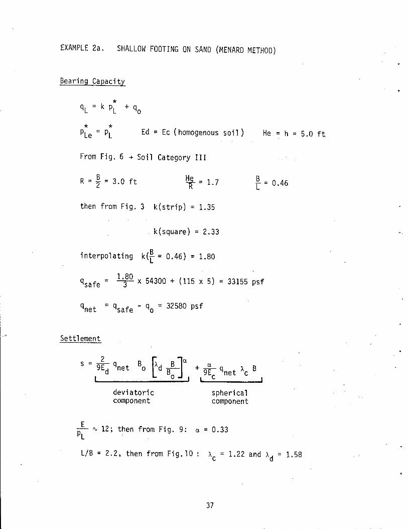
EXAMPLE 2a. SHALLOW FOOTING ON SAND (MENARD METHOD)
Bearing Capacity
Ed = Ec (homogenous soil) He = h = 5.0 ft
From Fig. 6 -+- Soil Category III
B R = '2 = 3.0 ft tlt = 1.7
B . r = 0.46
then from Fig. 3 k(strip) = 1.35
k(square) = 2.33
interpolating B k(r = 0.46) = 1.80
q = 1.80 x 54300 + (115 x 5) = 33155 psf safe 3
q = q - q = 32580 psf net safe 0
Settlement
deviatoric component
spherical component
PE ~ 12; then from Fig. 9: a = 0.33 L ..
LIB = 2.2, then from Fig. 10: Ac = 1.22 and Ad = 1.58
37

2 32580 6 0 0.33 0 33 32580 s = x 2. 0 x (1. 58 2.' 0 ) + -'9- x 9 689,000 689,000 x
1.22 x 6.0
s = .035 + .013 = . 048 ft < sall = .082 ft
therefore, use Pall = qsafe = 33155 psf
38

EXAMPLE 2b. SHALLOW FOOTING ON SAND (B.J.S. METHOD)
Bearing Capacity
Ed = Ec D = He = 5.0 ft
From Fig. 4 : Use chart for sand and gravel
~ = ~:~ = 0.83 * PL = 54300
* For a square footing: PL = 125300 psf + k = 2.64
* PL = 41770 psf + k = 2.55
* then for PL = 54300 psf + k = 2.56
Similarly, for a strip footing: k = 1.43
Interpolating with ~ = 0.46 + k = 1.95
q = 1.95 x 54300 + (115 x 5) = 35870 psf safe 3 .,~
qnet = 35295 psf
Settlement.
E/PL ~ 12, From Fig. 9 + a = 0.33
L/B = 2.2, From Fig. 10 + ~d: = 1.58 and ~c = 1.22
39

2 35295 6.0 0.33 0.33 35295 s = 9" 689,000 x 2.0 x(1.58 2.0) + -9- 689,000 x 1.22 x 6.0
s = .038 + .014 = .052 ft
s < sall' therefo~e, use Pall = qsafe ~ 35870 psf
40

EXAMPLE 2e. SHALLOW FOOTING ON SAND (B.G. METHOD)
.Beari Q9 Capacity
He = h = 5.0 ft
From Fig. 7 + Soil Category 3
~ = 1.7 B _ [ - 0.46
From Fig. 5: k(square) = 1.21
k(strip) = 1.11
Interpolating: k (~ = 0.46) = 1.16
q = 1.16 x 54300 + (115 x 5) = 21571 psf safe 3
qnet = 20996 psf
Settlement
2 B a. a. S = 9E qnet Bo ( Ad -B -) + 9E qnet \ B doe
E/PL ~ 12, then from Fig. 9 + a. = 0.33
Ed = Ec
L/B = 2.2, then from Fig. 10 + Ad = 1.58 and I.e = 1.22
2 20996 6.0 0.33 0.33 20996 s = 9 689,000 x 2.0 x (1.58 2.0) + -g-- 689,000 x 1.22 x 6.0
41

s = .023 + .008 = .031 ft
s < sall' therefore, use Pall = qsafe = 21571 psf
42

EXAMPLE PROBLEM 3:
STRIP 'FOOTING ON SAND
L = 33 ft.
Pl (pst) E(psf) B= 7 ft.
Yt = 124 pef t 50,100 451,000
5ft.
l--.l 5 · 39,700 . 343,000 I
35,500 326,000 silty
33,400 299,000 f sand
10 · . 3.5 ft. 2 37,400 372,000 t 52,200 428,000 3
15 ..
4 83,600 585,000
20 .~
61,600 524,000 5
62,700 520,000 6 25 ·
66,800 622,000 7.
30 83,500 693,000 8
z(ft,} z (ft.l
43

EXAMPLE 3 STRIP FOOTING ON SAND
Bearing Capacity
qL = k pte + qo
where pt i = [~ PL J 1 In " equi va 1 ent net 1 imit pressure
ptl = (50100 x 39700)1/2 = 44600
pt2 = (39700 x 35500 x 33400)'/3 = 35700
pt3 = 37400
pte = (44600 x 35700 x 37400)1/3 = 38600
n He = _1_ I: (pt. x z.):: equivalent embedment depth where 1 - n are
pte 1 I 1
layers within the actual depth of embedment 1
He = 38600 (50100 x 5.0) = 6.5 ft
Determination of k, (Menard)
From Fig. 6, silty sand + soil category 1
B 7.0 0 21 r = 33.0 = • he = 6.5 =
R 3.5 1.9
From Fig. 3: k(strip) = 1.11
k(square) = 1.58
B k(r = 0.21) = 1.30
qsafe = 1.~0 x 38600 + (124 x 5) +17347 psf

qnet = 16727 psf
Determination of k, (B.J.S.)
Q = 5.0 = 0 71 B 7.0 . B _ "[ - 0.21
From Fig. 4, sand and gravel:
* square footing + for PL = 41770; k = 2.4
* for PL = 20890; k = 2.0
* then, for PLe = 38600; k = 2.34
Similarly, for a strip footing:
* for PL = 41770; k = 1.35
* for PL ~ 8350; k = 1.10
* then, for PL = 38600; k = 1.31
Interpolating with ~ = 0.21 + k = 1.53
qsafe = 1353 x 38600 + (124 x 5) = 20306 psf
qnet = 19686 psf
Determination of k, (B.G.)
He = 6.5 ft ~ = 6.5 = 1 9 R 3.5 .
B L = 0.21
From Fig. 7 , Soil Category 2
45

From Fig. 5: k(square) = 1.11
k(strip) = 1.0
B k(r = 0.21) = 1.02
q = 1.02 x 38600 + (124 x 5) = 13744 psf safe 3
qnet = 13124 psf
Settlement
where Ec = harmonic mean of E's within layer 1
Ed = weighted average of E's from layers 1 - 16
3 1 1 1 Ec + Ic - 343,000 + 326,000 + 299,000
Ec = 321,632 psf
2 1 1 E2 = 299,000 + 372,000
E2 = 331,529 psf
=-~3_= 1 + 1 + 1 E3/ 4/ 5 428,000 585,006 524,000
E3/!/5 = 503,842 psf
46

3 1 1 1 ~E6--/~7/--8 = 520,000 + 622,000 + 693,000
E6/ 7/ 8 = 603,161 psf
E9/ 16 is taken as equal to E6/ 7/8· This is conservative since
modulus increases with depth.
4 1 1 1 1 Ed = 321,632 + 10.85){331,529) + 503,842 + (2.5){603,161) +
1 {2.5){603,161
Ed = 401,250 psf
Note: (0.85) and (2.5) are weighing coefficients used to indicate the
relative importance of the depth to the soil layers in question. E _d_ = 401,250 '" 10 P* 38600 Le
From Fig. 9 + ad = 0.33
E _c_ = 321,632 '" 8 P* 38600 Le
From Fig. 9 + ac = 0.33
L 33 6"=-,-=4.7 From Fig. 10 + Ad = 2.09 and Ac = 1.38
Settlement with Menard qnet:
2 16727 7.0 0.33 0.33 16727 s = 9" = 401,250 (2.0) (2.09 2.0) + -9- 321,632 (1.38) (7.0)
s = .036 + .018 = .054 ft
47
..

Settlement with B.J.S. qnet:
2 19686 7.0 )0.33 0.33 19686 s = 9 401,250 (2.0) (2.09 2.0 + --9-- 321,632 (1.38) (7.0)
s = .042 + .021 = .063 ft
Settlement with B.G. qnet:
2 13124 7.0 0.33 0.33 13124 s = 9 401,250 (2.0) (2.09 2.0 ) + --9-- 321,632 (1.38) (7.0)
s = .028 + .014 = .042 ft
48

EXAMPLE PROBLEM 4:
RECTANGULAR FOOTING ON LAYERED SOIL
L = 40 ft. • PL (pst) E{psf)
B = 16 ft.
33,500 246 10002: Yt = 102 pcf qo =612 psf 1
'7 - - - -6.0ft. l J ! !!
* 10 26,800 290,000 .. 37,900 446,000 I 8ft. = 8/2
! 37,900· 357,000
20 37,900 603,000 cloy 2 and marl
40,200 893,000
40,200 781,000
30 31,250 536,000 3 42,400 781,000
40,200 826,000
46,900 1,562,000 4 40
37,900 1,228,000
49,100 1,339,000 marl 5
51,300 1,562,000
50 51,300 1,674,000
67,000 1,897,000 6
It
z {ftl z (ttl
49

EXAMPLE 4. RECTANGULAR FOOTING ON A LAYERED SOIL (MENARD METHOD)
Bearing Capacity
where: 1
* * * * 3" PLe = (PLl x PL2 x PL3)
* PU"= 33500 psf 1
* ~ PL2 = (26800 x 37900 x 37900)~
* PL2 = 33415 psf
* k PL3 = (37900 x 40200) 2
* PL3 = 39033 psf 1
P~e = (33500 x 33415 x 39033) j
* so that:PLe = 34855 psf
1 n * 1 He = --:jC E (PU x ~zi ) = 34855 33500 x 6.0
PLe 1
He = 5.77 ft
From Fig. 6 + Soil Category II
B 16 [ = 40 = 0.40 "~= 5.77 = 072 R 8.00 .
From Fig 3 + k(square) = 1.32
k(strip) = 1.00
50

From Fig. 3 ~ k(~ = 0.40) = 1.13
qsafe = 1313
x 34855 + (6.0 x 10²) = 13741 psf
qnet = 13129 psf
Settlement
Ec = harmonic mean of Els within layer 1
3 _ 1 1 1 ~ - 290,000 + 446,000 + 357,000
Ec = 353,292 psf
Ed = weighted harmonic mean of Els from layers 1 - 16
E1 = Ec = 353,292 psf
2 _ 1 1 ~ - 603,000 + 893,000
E2 = 719,892 psf
8 _ 1 +.1 1 1 1 E3/ 4/ 5 - 781,000 536,000 + 781,000 + 826,000 + 1,562,000 +
1 + 1 + 1 1,228,000 1,339,000 1,562,000
E3/4/5 = 943,539 psf
2 1 + 1 ~ = 1,674,000 1,897,000
E6 = 1,778,537 psf
51

E6/ 8 and E9/ 16 are taken equal to E6 since no deeper modulus data
is available. This assumption is conservative if the modulus con-
tinues to increase with depth.
4 _ 1 111 Ed - 353,292 + (0.85)(719,892) + 943,539 + ....,....,{2:-....... 5),...,.(~1:....,7r=78=-,-=53=7~) +
1 ( 2.5)( 1,778,537)
Ed = 669,523 psf
~ = 669,523 ~ 19' From Fig. 9 + ad = 1.0 * 34855 ' PLe
Ec. = 353,292 ~ 10' From Fig. 9 + etc = 0.67 * 34855 ' PLe
~ = i~ = 2.5; From Fig. 10 + Ad = 1.82 and Ac = 1.25
2 34855 ( 16 )1. O. 0.67 34855 s = 9 659,523 (2.0) 1.82 2.0 + --9-- 353,292 (1.25)(16)
s = .337 + .147 = .484 ft
Recommend bearing pressure: Pall = .082 x 13741 .484
Pall = 2328 psf
52

EXAMPLE PROBLEM 5:
STRIP FOOTING WITH SOFT LAYER AT DEPTH
L = 33 ft.
P~ (psf) E(psf) B = 6.5 ft.
Yt = 124 pef j
50,100 451,000 5 ft.
I~ 5 39,700 343,000 I
35,500 326,000 - I silty 40,200 299,000 sond
t 10 3.25 ft. 2 41,800 372,000· t
52,200 428,000 3
15 . 14.75 ft.
4 soft 5850 58,500 silt
, layer 20
5640 52,400 5
20.75
62.700 520,000 6
25
66,800 622.000 7
30 83,500 693,000 8
~ It
z(ft') z(ft.}
53

EXAMPLE 5. STRIP FOOTING ON A SOFT LAYER AT DEPTH
Bearing Capacity
Estimate=
Silty sand, from Fig. 7 -+ Soil Category 2
.!!=~=02 L 33.0 . ¥ = i:~5 = 1.54
Now, from Fig. 5 -+ k(5quare) = 1.06
k(strip) = 1.02
k(~ = 0.2) = 1.03
* Assume that PLe is probably controlled by weak layer. (This is
conservatively false.)
* k PLe = (5850 x 5640) 2 = 5744 p5f
_ 1 ( ( qsafe - 3 1.03) (5744) + 5 x 124) = 2592 psf
qnet = 1972 p5f
Settlement
Here: 5 = 5' + 511
T
2 B CY. N Where: 5' - q B (, ) + ~ q - 9Ed n 0 Ad B 9E nAB o c c
54

· ,\,,:0 .. ... :j .•.. : •.
" (II) H s = a - - - IIp Ec Em c
From Example 3, Menard method yields Sl = .054 ft
Now consid~r the softness of the silt layer:
Ec = pressuremeter modulus of soft layer
2 1 1 Ec = 58500 + 52400
Ec = 55282 psf
Em = Ed = 401,250 psf (from Example 3)
Note: ~ _ ~ is a measure of the different hardnesses of the soil c m
layers in question.
From Boussinesq theory and Newmarkls chart, the vertical stresses at
the upper and lower surfaces of the soft layer have changed by:
z = 14.75 ft + llcrv = 0.24 qnet
z = 20.75 ft + llcrv = 0.17 qnet
qnet = 1972 psf (llOv) at 14.75 ft = 473 psf
(llov) at 20.75 ft = 335 psf
Average IIp = (473 + 335)/2 = 404 pst
" (II) H s = a - - - IIp Ec Em
E Pt = ~~~~2_ ~ 10, From Fig. 9. silt + a = 0.5
s" = 0.5 (55~82 - 401:250-)(404){20.75 - 14.75)
s" = 0.018 1
thus, sT = 0.054 1 + 0.018 1 ~ 0.0721
55

EXAMPLE PROBLEM 6:
MAT FOUNDATION ON A SOFT LAYER CLOSE TO GROUND SURFACE
B = 160 tt. p~ (pst) E (pst)
1.5 -----¢ 1.5 ft.1
5000 45,100 3.5 -----
3970 34,200
5.5 --- --3550 32,600
loose Yt = 124 pet silt
7.5 - - ---3760 29,900
9.5 10
-+-----+----------------9.5 ft.
shale
20
z(ftl z (ftl
56

EXAMPLE 6. MAT FOUNDATION ON A SOFT LAYER
Bearing Capacity
1 * Estimate qsafe = 3 k PLe + qo
Since ~e ~ 0 + k = 0.8
Assume that the silt layer controls bearing capacity; then let:
* PLe = average of the compressible layer
* ~ PLe = (5000 x 3970 x 3550 x 3760)4 = 4035 psf
qsafe = (~ x 0.8 x 4035) + (124 x 1.5) = 1262 psf
qnet = 1076 psf
Settlement
For a wide foundation underlain by a soft layer (i.e. relatively
thin, soft layer~
h () ~) () n ex. Bi p. s = f a z B F P z dz = r I 1 ~z. o E z) 1 Ei 1
For silt layer:
E ~ ~ 9, From Fig. 9 + a = 0.5 PL
* k p F = safety factor = . Le, where k = 0.8
qnet
57

4035 F = (0.8) 1076 = 3.0
2 F 2 3.0 thus, B(F) = 3 (F-l) = 3 (3.0-1.0) = 1.0
Assume that ~pv due to foundation loading is equal to actual
foundation pressure since layers of silt are thin compared to
foundation.
Then:
s = 0.124 ft
58

CHAPTER 5. - COMPARISON BETWEEN PREDICTED AND MEASURED BEHAVIOR
It has been shown in 3.1.1 that when the width of the footing (8) is
.small compared to the depth of the deposit (H), the major part of the
settlement is induced by the deviatoric tensor (very little consolidation
settlement). In section 3.1.6 and 3.1.7 special steps were taken to deal
with the cases where the width of the foundation (B) is large compared
to the thickness of the compressible layer (H); in this case the major
part of the settlement is due to consolidation (Figure 13). As a re
sult, the pressuremeter approach to settlement of shallow foundations is
recommended when HIB is large (2 or more); otherwise the pressuremeter
approach must be complemented by conventional consolidation tests.
Numerous comparisons of predicted versus measured settlement have
been made with the pressuremeter approach (1); they are presented in
Figures 14 through 16.
Experimental evidence for the bearing capacity factor k (shallow
foundation) can be found in references 6, 7, 8, and 1. The experimental
results are presented in Figure 17.
Figure 17 shows the design bearing capacity curves for the B.G. me
thod and the actual data points found through experiment by Menard (1).
In the investigation by Menard, the ultimate bearing capacity was con
sidered to be the pressure at a footing penetration of 1.6 inches.
The design curves shown on Figure 17 are the design curves of Busta
mante and Gianeselli (Figure 7).
59

B
p
H +
/77777)//// 777777777777/ 7777 77/
li»1 B
H
FIGURE 13: Pressuremeter Settlement Concepts
60

LO of
--c: Q)
E ~O. --Q) C/)
"0 Q)
of f
-o 0.25 of ~sf "0
Q) \,.,
a.
O~------~------~--____ ~ ____ ~ o
Legend o Clay o Sand t::. Sil t
* Other
0.25 0.50 0.75 Measured Settlement, em
e Embankment sf Strip Footing
r Raft f Individual Footing
1.0
FIGURE 14: PREDICTED VERSUS MEASURED SETTLEMENT (Very Small Settlement)
61

IO~----~----~----~----~ __ ~
E 8 u ..rc: Q)
E ..! 6 .. -CD en "C .! 4 .2 "C Q)
d: 2
fbcl
4 6 8
Measured Settlement, em ~ o Cloy [J Sand, A Silt * Other
e Embankment sf Strip Footing r Raft f Individual Footing
10
FIGURE 15: PREDICTED VERSUS MEASURED SETTLEMENT (Moderate Settlement)
62

E o .. -
.... ' . ." -: .' ~ , .. ,'.-. .' ,-: "-.
2
150
~ 100 E G)
= -G)
en "'C G) -o .-"'C G) ... 0.
~gend o Clay oSand t:. Silt .Other
oe
50 100 150
Measured Settlement, em
e Embankment sf Stri p Footing r Raft f Individual Footing
FIGURE 16 : PREDICTED VERSUS MEASURED SETTLEMENT (Large Settlement)
63
200

· ........ ; .... . ":':.; ...... ;.'. - ....
k for Sha Ilow Foundations
3r-----+-----~-----+----~------~-----
o Silt c Sand
Circular or Square ~ __ -+-___ +-__ --.-_S_tri P .,..----f----
CI CI
CI
CI 2r-----~----~~----;-----~------~------
CAT. I
o------~--~~--~----~--~--~--~~~--o 2 4 5 He -
R
FIGURE 17 : Comparison of the Bearing Capacity Factors Predicted by the B.G. Method and Measured by Menard (References 1, 6, 7, 8),
64
•
..
..
- --- ------------------------------

REFERENCES
1. Baguelin, F., Jezequel, J.-F., and Shields, D. H., liThe Pressuremeter and Foundation Engineeringll, Trans-tech Publication, Rockport, Mass., 1978.
2. Briaud, J.-L., liThe Pressuremeter: Application to Pavement Design ll , Ph.D. Dissertation Civil Engineering Department, University of Ottawa, Canada.
3. Bustamante, M., and Gianeselli, L., Portance Reel1e et Portance Cal-culee des Pieux Isoles,'Sollicit Verticalement ll , Revue Francaise de Geotechnigue, No. 16, August, 1981.
4. Kahle, J. G., IIPredicting Settlement in Piedmont Residual Soil With the Pressuremeter Test,1I presented at the Transportation Research Board Meeting, Washington, January 1983.
5. Menard, L., Rousseau, J., "LI Evaluation des Tassements, Tendances Nouvelles", Sols - Soils No.1, 1962.
6. Menard, L., "Calcul de la Force Portante des Fondations sur 1a Base des Resu1tats des Essais Pressiometriques ll
,' Sols - Soils No.5. 1963.
7. Menard, L., "Ca1cul de 1a Force Portante des Fondations sur 1a Base des Resultats des Essais Pressiometriques: Resultats Experlmentaux et Conc1usions", Sols - Soils No.6, 1963.
8. Menard, L., "Etude Experimenta1e du Tassement et de 1a Force Portante des Fondations Superficiel1es ll , Sols - Soils No. 10, Septembre, 1964.
9. Menard, L., IILe Tassement des Fondations et 1es Techniques Pressiometri ques II , Anna 1 es ITBTP, Pari s, Supplement No. 288, Decembre, 1971.
10. Menard, L., liThe Menard Pressuremeter: Interpretation .and Application of Pressuremeter Test Results to Foundation Design ll
, General Memorandum, Sols - Soils, No. 26, 1975.
11. Schmertman, J. H., IIStati c Cone to Compute Stati c Settl ement over Sand," Journal of the Soil Mechanics and Foundation Engineering Division of ASCE, Vol. 96, 5M3, 1970.
12. Schmertman, J. H., "Improved Strain Influence Factor Diagram," Technical Note, Journal of the Soil Mechanics and Foundation Engineering Division of ASCE, Vol. 104, No. BT8, August 1978.
65