1

Technical Support for the Analysis of Historical Flow Data from Selected Flow Gauges in the Trinity, San Jacinto, and

Adjacent Coastal Basins

Galveston Bay Salinity Zonation Analysis

for the

Trinity-San Jacinto and Galveston Bay Basin and Bay Expert Science Team

Submitted to:

Trinity –San Jacinto BBEST

Prepared by:

Espey Consultants, Inc. 3809 S. 2nd St. Suite B-300

Austin, TX 78704

and

Trungale Engineering & Science 707 Rio Grande, Suite 200

Austin, TX 78701

August 2009

2

i

Table of Contents 1.0 Introduction............................................................................................................. 1 2.0 Assessment of Spatial and Temporal Characterizations of Salinity-Flow Methods for Galveston Bay ............................................................................................................... 2

2.1 Flow Comparison Analysis................................................................................. 3 2.2 Comparative Statistical Analyses ..................................................................... 11

3.0 Evaluation of Pre-Reservoir Flow Patterns........................................................... 22 4.0 Development of Salinity-Ecology Relationships.................................................. 26 5.0 Preliminary Flow Evaluation for Desired Salinity Conditions ............................. 29 6.0 Conclusions........................................................................................................... 45 7.0 References............................................................................................................. 47 Appendices Appendix A: Pre-Post Reservoir Flow Patterns Appendix B: Salinity-Ecology Workshop 1 Appendix C: Salinity-Ecology Workshop 2 Appendix D: Isohaline Plots Appendix E: Historical Salinity Zone Area Analyses Appendix F: Historical Flow Ogives Appendix G: Response to Comments

ii

List of Figures Figure 2.1 TWDB Datasonde Locations ........................................................................................................ 2 Figure 2.2 Correlation Plot for Total Galveston Bay Watershed Representations ......................................... 6 Figure 2.3 Correlation Plot for Trinity Watershed Representations ............................................................... 6 Figure 2.4 Correlation Plot for San Jacinto Watershed Representations........................................................ 7 Figure 2.5 Time Series Plot for Total Galveston Bay Watershed Representations ........................................ 8 Figure 2.6 Time Series Plot for Trinity Watershed Representations .............................................................. 8 Figure 2.7 Time Series Plot for San Jacinto Watershed Representations....................................................... 9 Figure 2.8 Comparison of Monthly Flows between Period of Record (1941-2005) and Model Period (1983-2005)............................................................................................................................................................. 11 Figure 2.9 TWDB Datasonde Locations (Green) and Daily Modeled Locations (Red), and Monthly Modeled Locations (Black) .......................................................................................................................... 12 Figure 2.10 Univariate Logarithmic Regressions at Trinity ........................................................................ 13 Figure 2.11 Univariate Logarithmic Regressions at Redbluff ..................................................................... 14 Figure 2.12 Univariate Logarithmic Regressions at Dollar and Midgal....................................................... 14 Figure 2.13 Univariate Logarithmic Regressions at Bolivar ........................................................................ 15 Figure 2.14 Time series comparison at Trinity............................................................................................. 15 Figure 2.15 Time series comparison at Redbluff.......................................................................................... 16 Figure 2.16 Time series comparison at Dollar and Midgal ......................................................................... 16 Figure 2.17 Time series comparison at Bolivar........................................................................................... 17 Figure 2.18 Spatial Depiction of Modeled Salinities.................................................................................... 20 Figure 2.19 Percent of Bay Area with 5 PSU bins and associated Historical Hydrograph .......................... 21 Figure 3.1 Monthly Medain Flow Pre- and Post- 1968 (Lake Livingston Impoundment) ........................... 22 Figure 3.2 Annual Flow (ACFT/YR) at Trinity Rv at Romayor about 11th percentile annual flow based on full POR (25-09)........................................................................................................................................... 24 Figure 3.3 Annual Flow (ACFT/YR) at Trinity Rv at Romayor about 48th percentile annual flow based on full POR (25-09)........................................................................................................................................... 24 Figure 3.4 Annual Flow (ACFT/YR) at Trinity Rv at Romayor about 91th percentile annual flow based on full POR (25-09)........................................................................................................................................... 25 Figure 4.1 Map of Identified Species Regions for Galveston Bay ............................................................... 28 Figure 5.1 Example 1-year Depiction of Spatial Variability in Salinity Zone (2-10 psu) ............................ 30 Figure 5.2 Historical Seasonal Frequency of Occurrence of Atlantic Rangia Salinity Zone Area (2-10 psu)...................................................................................................................................................................... 33 Figure 5.3 Historical Seasonal Frequency of Occurrence of Gulf Menhaden Salinity Zone Area (5-15 psu) in Spring ....................................................................................................................................................... 33 Figure 5.4 Historical Relation between Monthly Salinity Zone Area for Atlantic Rangia and Trinity Watershed Monthly Flow - Spring ............................................................................................................... 34 Figure 5.5 Historical Relation between Salinity Zone Area for Atlantic Rangia and Trinity Watershed Monthly Flow - Summer .............................................................................................................................. 34 Figure 5.6 Historical Relation between Salinity Zone Area for Atlantic Rangia and Trinity Watershed Monthly Flow - Fall...................................................................................................................................... 35 Figure 5.7 Least-squares Fit Step Function for Atlantic Rangia Salinity Zone Area related to Trinity River Watershed Monthly Flows – Spring (2-10 psu)............................................................................................ 35 Figure 5.8 Least-squares Fit Step Function for Atlantic Rangia Salinity Zone Area related to Trinity River Watershed Monthly Flows – Summer (2-10 psu)......................................................................................... 36 Figure 5.9 Least-squares Fit Step Function for Atlantic Rangia Salinity Zone Area related to Trinity River Watershed Monthly Flows – Fall (2-10 psu) ................................................................................................ 36 Figure 5.10 Historical Monthly Trinity River Watershed Flow Ogive for Spring (1983-2005)................... 39 Figure 5.11 Historical Monthly Trinity River Watershed Flow Ogive for Summer (1983-2005)................ 39 Figure 5.12 Historical Monthly Trinity River Watershed Flow Ogive for Fall (1983-2005) ....................... 40 Figure 5.13 Historical Monthly Trinity River Watershed Flow Ogive for Winter (1983-2005) .................. 40 Figure 5.14 Historical Relation between Salinity Zone Area for Vallisneria and Trinity Watershed Monthly Flow - Fall .................................................................................................................................................... 44

iii

List of Tables Table 2.1 TWDB Datasondes........................................................................................................................ 3 Table 2.2 TxBLEND vs. TWDB Difference in Total Galveston Bay Inflows ............................................... 4 Table 2.3 TxBLEND Original vs. New Difference in Total Galveston Bay Inflows ..................................... 5 Table 2.4 TxBLEND Original vs. New Hydrologic Inputs ............................................................................ 5 Table 2.5 Annual Flow Volume Rankings ................................................................................................... 10 Table 2.6 Model Goodness of Fit at Trinity ................................................................................................. 18 Table 2.7 Model Goodness of Fit at Redbluff .............................................................................................. 19 Table 2.8 Model Goodness of Fit at Dollar and Midgal ............................................................................... 19 Table 2.9 Model Goodness of Fit at Bolivar ................................................................................................ 19 Table 3.1 Annual Flows Pre- and Post - 1968 (Lake Livingston) ................................................................ 23 Table 4.1 Preliminary Identified Biological Indicators for Galveston Bay .................................................. 27 Table 4.2 Seasonal Assignment of Months .................................................................................................. 28 Table 5.1 Percentiles of Monthly Area (ha.) for Atlantic Rangia Salinity Zone (2-10 psu)......................... 32 Table 5.2 Percentiles of Monthly %Area for Atlantic Rangia Salinity Zone (2-10 psu) .............................. 32 Table 5.3 Selected Seasonal Maximum Salinity Zone Areas (ha.) for Atlantic Rangia (2-10 psu).............. 37 Table 5.4 Example Seasonal Flow Range for Trinity River Watershed based upon 68% Prediction Intervals for Maximum Area Historical Frequency Atlantic Rangia Salinity Zone (2-10 psu)................................... 38 Table 5.5 Example Flow Matrix for Trinity River Watershed for Atlantic Rangia (2-10 psu) .................... 38 Table 5.6 Example Preliminary Flow Matrix for the Trinity River Basin.................................................... 41 Table 5.7 Example Preliminary Flow Matrix for the San Jacinto River Basin............................................. 42

iv

1

1.0 Introduction Galveston Bay is the largest estuary on the Texas coast (approximately 600 square miles, or 384,000 acres), with numerous economically and ecologically important organisms utilizing habitat areas within the system as a nursery, and various habitat types providing sufficient conditions for survival and development (Minello 1999, Weinstein 1979). Freshwater inflow demonstrates its ecologically important functional roles in several ways: through the transportation of sediments and nutrients; the maintenance of varying salinity gradients; maintenance of wetlands, plant, and animal productivity; and the maintenance of economically important fish and shellfish populations. The principal freshwater inflows to the Galveston Bay system originate from the Trinity and San Jacinto river basins, and the coastal watershed contributing to the estuarine system. One of the principal mandates set forth by Senate Bill 3 (SB3) to the Trinity-San Jacinto and Galveston Bay Basin and Bay Expert Science Team (BBEST) states that the BBEST shall, “[d]evelop environmental flow analyses and a recommended environmental flow regime…”. An “environmental flow regime” is defined by SB3 as:

“a schedule of flow quantities that reflects seasonal and yearly fluctuations that typically would vary geographically, by specific location in a watershed, and that are shown to be adequate to support a sound ecological environment and to maintain the productivity, extent, and persistence of key aquatic habitats in and along the affected water bodies.”

Recalling that definition as one that reflects seasonal and yearly fluctuations, fundamental to the proposed approach herein is the recognition of one of the dramatic features of the climate of Texas; namely, its pronounced geographical variation, which leads to a marked decline in precipitation and river flow from east to west across the state (Ward, 2000). This decline in flow from east to west can in fact be characterized as a variation in frequency of the salinity regime, wherein flow varies inter- and intra-annually. These flow regimes, arriving at varying frequencies to each estuarine system, can indeed be characterized as delivering a corresponding salinity regime to each estuary, from the Sabine (where the system is frequently fresh), to the upper Laguna-Madre (where the system is frequently saline). Organisms have adapted over time to succeed within these estuarine systems’ variable salinity conditions, and it is the characterization of the range and frequency of these conditions which has been identified by the Trinity-San Jacinto BBEST as one critical factor to the maintenance of the ecological health of Galveston Bay’s estuarine environment. This project report describes work performed under a scope of work developed by the Trinity-San Jacinto BBEST to be used in part to support the development of recommended flow quantities and a flow regime supportive of a sound ecological environment for the Galveston Bay system. A fundamental aspect to the development of a flow recommendation for Galveston Bay is the relation of inflows necessary to maintain specified salinity conditions sufficient for organisms inhabiting the system;

2

more specifically, precisely defined areas identified throughout the bay. It is important to understand the historical salinity regimes in these areas, and their relationships to freshwater inflows from the Trinity, San Jacinto, and coastal watersheds. Thus it has been the primary objective of this study is to characterize historical spatial and temporal salinity conditions in Galveston Bay, and determine whether the relationship between freshwater inflow from the Trinity and San Jacinto Rivers and these salinity patterns can be accurately and robustly combined with ecological data. A secondary objective of this study has been the identification of appropriate biological indicators representative of the ecological characteristics of Galveston Bay that can be utilized to specify salinity ranges and associated flow regimes to which these organisms respond.

2.0 Assessment of Spatial and Temporal Characterizations of Salinity-Flow Methods for Galveston Bay

Prior to the development of a historical depiction of salinities, an investigation was made into the ability of the Texas Water Development Board’s TxBLEND 2-dimensional hydrodynamic salinity model for Galveston Bay to accurately reproduce observed conditions via comparison with data collected through the TWDB datasonde program. Four locations have been evaluated within this investigation to assess model capability: Trinity Bay, Red Bluff, Dollar Pt/MidGal, and Bolivar (located in Figure 2.1).

Figure 2.1 TWDB Datasonde Locations

3

The TWDB datasonde data have been utilized within this analysis and the periods of record are indicated in Table 2.1 below. As can be seen in this table, in order to sufficiently capture an adequate period of record for analysis it has been deemed necessary to combine the Dollar and MidGal gages for this assessment. Ultimately this is suspected to contribute to the variance to any solution, and as further data is developed at the MidGal gage over time this will be one aspect that could be improved in subsequent analyses.

Table 2.1 TWDB Datasondes

Sonde Name Period of Record Trinity Bay 1986-2000, 2004-2007 Red Bluff 1990-1999 MidGal 2001-2007 Dollar 1987-2000 Bolivar 1987-2007

Prior to any flow/salinity analyses, a rudimentary QA/QC was performed on the raw hourly sonde data wherein spurious and suspect values (e.g. entries of -9.99, continuous 0 values for extended periods of time where sonde exposure is suspected, redundant, and non-salinity data) were removed, and daily averages subsequently calculated without regard for the depth at which they were collected. In some cases data were removed based on comparison to spot check measurements made by the TWDB. Daily hydrologic data for all of the contributing watersheds to the Galveston Bay system were acquired from the TWDB. These data represent USGS gaged flows, ungaged flows as calculated by the TWDB’s Texas Rainfall Runoff model (TxRR), and reported diversions and discharge amounts downstream of the gaged locations.

2.1 Flow Comparison Analysis In the process of comparative analysis of TxBLEND and datasonde salinity data, a discrepancy in inflow data was found between the hydrologic representations for the contributing watersheds utilized by the TWDB within the Galveston Bay TxBLEND input data and hydrologic data reported on the TWDB website for the Total Galveston system(http://midgewater.twdb.state.tx.us/bays_estuaries/hydrology/galvestonsum.txt). The difference in these reported monthly flows is displayed in Table 2.2. From this comparison it can be seen that over the entire period of record (1977-2005), 21% of months exhibit a difference greater than -10% and 1% of months exhibit a difference greater than +10%. With the 1991-1994 period excluded, 12% of months exhibit a difference greater than -10% and 2% of months exhibit a difference greater than +10%. Prior to 1991, 6% of months exhibit a difference greater than -10% and 2% of months exhibit a difference greater than +10%. After 1994, 19% of months exhibit a difference greater than -10% and 2% of months exhibit a difference greater than +10%.

4

Through communications of this discrepancy with TWDB staff, it was determined that the Total Galveston Bay hydrologic data reported on the TWDB website has been in error, as it potentially represents old estimations of flows from Lake Houston based on an incorrect datum.

Table 2.2

TxBLEND vs. TWDB Difference in Total Galveston Bay Inflows

January February March April May June July August September October November December1977 -7.8% -1.2% -6.2% 2.2% -5.2% -6.5% -2.1% -3.4% -5.0% -2.5% -5.1% -4.9%1978 -3.5% 0.1% -9.0% 0.5% 1.0% 2.9% -0.5% -0.1% -3.5% -1.8% -5.3% -14.3%1979 2.9% 3.8% -2.2% 12.3% -0.9% 2.8% -4.9% -8.5% 2.5% -10.2% -6.2% -5.7%1980 -3.9% -0.4% -3.1% -5.1% -0.6% -8.1% -5.5% -2.1% -6.8% -5.0% -3.9% -5.6%1981 -4.5% -3.7% -8.6% -4.3% 1.5% -0.7% -2.8% -5.4% -3.2% -4.7% -2.3% -4.9%1982 -7.3% -8.1% -6.8% 2.6% 6.2% -1.2% -0.5% -1.1% -0.2% -2.6% -1.4% -4.0%1983 -6.1% 0.4% 1.4% -8.3% 17.9% -8.2% -5.1% 2.3% -4.6% -20.3% -12.8% -2.4%1984 -7.3% -1.6% -4.5% -6.9% -3.5% -10.4% -8.4% -0.9% -3.0% 1.2% -4.7% -3.9%1985 -2.4% 1.4% 0.7% -7.0% -3.1% -5.7% -11.4% -3.7% -6.3% -5.3% 4.9% 1.5%1986 -15.6% -0.1% -10.2% 0.1% -0.8% 3.7% -5.2% -0.8% -4.3% -7.8% -3.6% 0.7%1987 -3.3% -2.8% -0.3% 0.4% -6.3% 3.6% -2.9% -0.3% -5.9% -7.9% 3.5% -6.0%1988 -6.3% -11.0% -4.1% -7.7% -6.6% -1.7% -2.8% -2.4% -7.5% -0.9% -1.1% -1.7%1989 -3.5% -7.7% -2.1% -4.0% 12.2% -0.8% -2.8% -4.3% -1.8% -5.5% -5.2% -1.9%1990 -2.8% -1.6% -2.2% -1.9% -1.6% -1.3% -2.8% -0.7% -4.5% -4.3% -2.3% -4.2%1991 -14.0% -21.5% -40.1% -15.4% -25.9% -30.3% -50.2% -48.8% -39.5% -51.7% -17.6% -14.6%1992 -10.5% -9.2% -10.1% -21.9% -26.9% -19.9% -47.2% -56.9% -33.0% -5.0% -26.0% -22.9%1993 -20.5% -28.3% -14.3% -20.4% -21.4% -14.1% -43.4% -61.6% -76.2% -5.8% -4.7% -8.4%1994 -10.5% 1.6% -1.5% -10.1% -3.3% -5.8% -10.4% -10.9% -15.1% -0.3% -2.3% -1.3%1995 0.5% -6.9% -1.4% -0.7% -3.4% -5.0% -10.4% -11.9% -25.3% -13.2% -17.1% -5.8%1996 -18.8% -28.7% -19.1% -7.6% -17.4% -5.2% -17.2% -9.9% -6.8% -14.2% -4.9% -3.4%1997 -4.4% 1.9% 0.2% -0.7% -1.6% -2.8% -11.0% -8.9% -5.5% -5.9% -9.4% -2.3%1998 0.4% -1.4% 2.2% -0.1% -9.6% -4.4% 0.8% -6.8% -7.8% 8.2% 16.1% -2.0%1999 -6.0% -3.3% -6.0% -3.9% -7.8% -4.2% -5.9% 2.0% -3.9% -4.6% 0.2% -5.6%2000 -3.5% -0.4% -1.0% -7.8% -4.4% -3.7% 0.2% 2.6% -3.4% -1.5% -0.7% -3.6%2001 -0.6% -1.9% -0.9% -8.1% -7.0% 3.4% -12.8% -10.3% -7.0% -1.8% -2.4% 1.5%2002 -5.0% -3.3% -7.4% -0.9% -3.5% -8.3% -6.7% -7.7% -7.9% 2.0% 11.0% -1.1%2003 -1.1% 3.2% -2.4% -12.3% -16.9% -7.4% -11.7% -13.2% -9.3% -5.0% 3.4% -11.6%2004 -0.2% 0.0% -6.3% -7.2% 0.0% -2.0% -0.6% -5.8% -10.1% -5.6% 1.4% -3.2%2005 -2.9% 3.2% -4.3% -8.3% -11.7% -14.0% -8.4% -16.9% -9.1% -15.9% -18.8% -9.3%

Subsequent to this assessment, new representations of the hydrology were provided by TWDB correcting for the above mentioned discrepancy. Some adjustments to the inflow dataset were made by TWDB as a result of improvements to the rainfall-runoff calculations and updated diversion and return data. Comparisons were next carried out between the original and new TxBLEND flow inputs. Monthly differences between the original and new TxBLEND inputs are presented in Table 2.3. The comparison between the original and new TxBLEND inputs indicates that over the entire period of record (1977-2005), 5% of months exhibit a difference greater than -10% and 3% of months exhibit a difference greater than +10%. The above comparisons display comparisons of the monthly inflow data for the Total Galveston Bay watershed. Further comparisons were carried out with daily inflow inputs for several of the component watershed areas contributing to the Galveston Bay system, including the Total Galveston Bay watershed, the Trinity watershed, and the San Jacinto watershed. The comparison results between original and new TxBLEND hydrologic inputs are presented in Table 2.4.

5

Table 2.3 TxBLEND Original vs. New Difference in Total Galveston Bay Inflows

January February March April May June July August September October November December

1977 -2.2% -0.9% -0.3% -0.9% -0.7% -3.7% -2.5% -3.5% -5.0% -2.5% -5.1% -4.9%1978 -3.8% -1.5% -0.2% -0.7% -0.4% -1.0% -1.3% -0.6% -3.5% -2.0% -4.7% -1.9%1979 -1.2% -1.5% -1.8% -1.7% -1.6% -0.8% -5.0% -1.9% -3.4% -1.7% -2.4% -0.8%1980 -3.8% -0.7% -3.1% -1.1% -1.7% -2.2% -6.3% -2.6% -6.8% -1.8% -3.5% -5.1%1981 -4.6% -3.7% -2.3% -4.1% -0.4% -3.2% -2.1% -5.2% -4.7% -2.5% -0.8% -0.4%1982 -2.3% -2.0% -0.8% -0.7% -0.7% -0.3% -0.4% -1.5% -0.4% -2.6% -2.1% -4.0%1983 -3.0% -2.2% -0.8% -0.4% -0.4% -3.4% -4.5% -3.9% -5.2% -0.8% -2.1% -2.0%1984 -3.3% -1.0% -0.3% -0.2% -2.1% -1.3% -0.5% -1.2% -3.0% -1.8% -1.4% -0.5%1985 -0.4% -2.2% -2.0% -0.4% -1.7% -4.2% -7.6% -3.7% -6.3% -3.9% -1.4% -0.3%1986 -0.8% -0.4% -0.4% -0.3% -0.3% -0.8% -0.1% -1.5% -3.3% -4.2% -3.2% 0.7%1987 6.1% -2.1% -0.3% -0.2% -6.2% -1.3% -2.5% -0.9% -6.1% -9.1% -5.0% -4.3%1988 -1.8% -1.0% -1.4% -3.9% -4.8% -1.9% -2.8% -2.5% -7.6% -0.9% -1.1% -1.8%1989 -3.2% -0.4% -0.6% -0.2% -0.5% -2.8% -2.5% -2.8% -1.9% -5.6% -5.3% -1.9%1990 -2.2% -0.7% -1.0% -1.2% -1.0% -0.1% -2.8% -0.7% -4.5% -4.2% -2.4% -4.2%1991 -2.0% -2.4% -1.2% -1.9% -2.9% -2.7% -6.4% -5.6% -7.3% -2.6% -1.4% -1.6%1992 -1.4% -1.4% -0.2% -1.7% -1.7% -1.7% -1.1% -0.9% -2.0% -1.0% -3.3% -1.5%1993 -2.3% -1.5% -1.5% -1.8% -2.1% -2.4% -0.1% -0.5% -3.0% -2.1% -0.3% -0.2%1994 0.2% 0.3% 0.1% -0.6% -1.2% 0.0% -1.7% -9.0% -5.4% -1.5% -0.1% -1.0%1995 -0.7% -0.7% -1.3% -0.3% -0.4% -0.8% -2.5% -6.0% 0.2% -2.9% -4.1% -4.0%1996 -5.0% 1.6% 1.1% -1.6% 4.1% 0.8% 1.4% -5.8% -4.7% 1.5% 4.8% 0.5%1997 -0.6% -0.6% -0.8% -1.3% -2.0% -2.4% -2.2% -5.5% -6.6% 1.2% 1.3% -1.3%1998 -1.4% 0.1% 1.2% 4.1% 30.5% 12.6% 14.8% 4.3% -3.0% -2.1% -0.6% -0.7%1999 -0.9% -0.4% -0.6% -0.2% -2.8% -1.5% -4.6% 3.7% -7.0% -6.2% -1.6% -6.4%2000 -18.9% -13.0% -10.5% -5.7% -5.7% -1.8% -7.7% -15.4% -20.5% -21.4% -6.2% 0.0%2001 -0.2% -1.0% -1.2% 81.9% -2.0% -0.8% 38.8% 4.9% 20.7% -4.5% -1.4% -2.6%2002 -2.7% -0.7% -3.1% -2.5% -2.2% -8.1% -7.5% -9.0% -6.6% -3.4% -2.9% -3.6%2003 -4.3% 0.1% -0.6% -5.7% -11.9% -8.1% 18.8% 11.8% 12.1% -7.7% -10.3% -10.9%2004 -7.2% -12.6% -10.5% -15.2% -7.8% -8.0% -1.2% -5.2% -7.4% 6.1% -7.2% 2.1%2005 -0.7% -4.9% -5.3% -4.2% 4.7% 5.3% -30.9% -20.9% -18.2% 0.5% -21.3% -12.0%

Table 2.4

TxBLEND Original vs. New Hydrologic Inputs

< -10% > +10%TGALB 7.4% 3.2%TRNTY 12.8% 0.6%SNJAC 0.5% 5.9%

TxBLEND Original vs. New Percentage of Days with Difference

Correlation plots between the different input sources are shown in Figures 2.2-2.4, with points yielding differences greater than +/- 10% highlighted in red. A perfect fit would result in a cluster of points along the diagonal line.

6

Total Galveston Bay

0

200,000

400,000

600,000

800,000

1,000,000

0 200,000 400,000 600,000 800,000 1,000,000TxBLEND Original

(ac-ft/d)

TxB

LEN

D N

ew(a

c-ft/

d)

Figure 2.2 Correlation Plot for Total Galveston Bay Watershed Representations

Trinity Watershed

0

100,000

200,000

300,000

400,000

500,000

0 100,000 200,000 300,000 400,000 500,000TxBLEND Original

(ac-ft/d)

TxB

LEN

D N

ew(a

c-ft/

d)

Figure 2.3 Correlation Plot for Trinity Watershed Representations

7

San Jacinto Watershed

0

100,000

200,000

300,000

400,000

500,000

0 100,000 200,000 300,000 400,000 500,000

TxBLEND Original(ac-ft/d)

TxB

LEN

D N

ew(a

c-ft/

d)

Figure 2.4 Correlation Plot for San Jacinto Watershed Representations

An assessment of the timing of these points, as displayed in Figures 2.5-2.7, indicates that a majority of the discrepancies occurred after the year 2000. In Total Galveston bay, 70% of months with differences higher than 10% occurred post 2000. In Trinity watershed, 83% of months with differences higher than 10% occurred post 2000. In San Jacinto watershed, 100% months with differences higher than 10% occurred post 2000. Thus the model calibration, the period of which was from 1989-1996, was determined to not be affected by this discrepancy in inflow data found between the original and more recent TxBLEND hydrologic inputs. The model was then re-run with the best available inflow data.

8

Comparative Time Series Plot of Total Galveston Bay Amounts

1

10

100

1,000

10,000

100,000

1,000,000

1/1/

1977

12/2

2/19

78

12/1

1/19

80

12/1

/198

2

11/2

0/19

84

11/1

0/19

86

10/3

0/19

88

10/2

0/19

90

10/9

/199

2

9/29

/199

4

9/18

/199

6

9/8/

1998

8/28

/200

0

8/18

/200

2

8/7/

2004

Date (Month)

Flow

(ac-

ft)

TxBLEND_OriginalTxBLEND_New

Figure 2.5

Time Series Plot for Total Galveston Bay Watershed Representations

Comparative Time Series Plot of Trinity Watershed Amounts

1

10

100

1,000

10,000

100,000

1,000,000

1/1/

1977

12/2

2/19

78

12/1

1/19

80

12/1

/198

2

11/2

0/19

84

11/1

0/19

86

10/3

0/19

88

10/2

0/19

90

10/9

/199

2

9/29

/199

4

9/18

/199

6

9/8/

1998

8/28

/200

0

8/18

/200

2

8/7/

2004

Date (Month)

Flow

(ac-

ft)

TxBLEND_OriginalTxBLEND_New

Figure 2.6 Time Series Plot for Trinity Watershed Representations

9

Comparative Time Series Plot of San Jacinto Watershed Amounts

1

10

100

1,000

10,000

100,000

1,000,000

1/1/

1977

12/2

2/19

78

12/1

1/19

80

12/1

/198

2

11/2

0/19

84

11/1

0/19

86

10/3

0/19

88

10/2

0/19

90

10/9

/199

2

9/29

/199

4

9/18

/199

6

9/8/

1998

8/28

/200

0

8/18

/200

2

8/7/

2004

Date (Month)

Flow

(ac-

ft)

TxBLEND_OriginalTxBLEND_New

Figure 2.7 Time Series Plot for San Jacinto Watershed Representations

10

Subsequent to the completion of the flow assessment, a long term simulation was conducted to provide salinity values under a wide range of inflow conditions. The model was originally calibrated for the period from 1987-1996 which was a relatively wet period. Table 2.5 which show the rankings in terms of annual flow volumes. The percent rank is based on the full period of annual inflow estimates beginning in 1941 (a 0% rank would indicate the lowest inflow year, 100% the highest). In order to simulate a period with a wider range of flow conditions the period from January 1983 through December 2005 was modeled. As an aid in identifying period types, pink indicates the driest third, yellow equates to the middle third, and green equals the wettest third.

Table 2.5

Annual Flow Volume Rankings

Year Surf.In. PerecentRank1983 13,248,081 64%1984 7,795,042 34%1985 12,491,535 59%1986 13,277,419 66%1987 9,988,234 44%1988 3,954,690 8%1989 12,530,243 61%1990 14,394,320 73%1991 22,598,609 97%1992 25,148,391 100%1993 19,951,721 91%1994 16,462,970 80%1995 15,484,064 77%1996 5,156,988 17%1997 16,811,926 83%1998 18,223,638 86%1999 7,112,886 28%2000 6,973,234 27%2001 24,324,853 98%2002 15,609,910 78%2003 11,666,127 56%2004 16,486,943 81%2005 8,058,561 38%

As can be seen from the comparison of the monthly flow ogives for the period of record and this modeled period (Figure 2.8 below), the two historical periods compare fairly well, with the 1941-2005 period appearing moderately wetter. This provides a means to place perspective on model results when considering the longer time period from 1941-2005.

11

0.0

0.1

0.2

0.3

0.4

0.5

0.6

0.7

0.8

0.9

1.0

10,000 100,000 1,000,000 10,000,000

Flow

Perc

enta

ge o

f Exc

eeda

nce

1983~2005 Flow

1941~2005 Flow

Figure 2.8

Comparison of Monthly Flows between Period of Record (1941-2005) and Model Period (1983-2005)

2.2 Comparative Statistical Analyses A long term simulation of the TxBLEND hydrodynamic model for Galveston Bay was conducted to provide estimated salinity values under a wide range of inflow conditions for the period from January 1983 through December 2005. Comparisons of the results of this simulation to observed sonde data are presented and utilized herein to conduct a model fit analysis and assess the utility of the model for further application to the development of characteristic salinity-zones within the Galveston Bay system. The modeled locations, along with the four datasonde locations utilized within this investigation are shown in Figure 2.9 below. The TxBLEND model is a 2-dimensional finite element model developed by TWDB (Matsumoto 1992) to simulate water circulation and salinity conditions in Texas Estuaries. The model uses triangular elements with linear basis functions to simulate salinity in two dimensions. Water circulation is simulated by simultaneously solving shallow water equations (continuity and momentum) and the salinity condition is solved by the mass transport equation or the convective-diffusion equation. The TxBLEND model itself is an expanded version of the BLEND model which was derived from an earlier model called FLEET (Grey 1987).

12

Figure 2.9

TWDB Datasonde Locations (Green) and Daily Modeled Locations (Red), and Monthly Modeled Locations (Black)

TxBLEND has been applied on all of the major bays in Texas primarily as part of the state methodology to determine freshwater inflow needs at the direction of 69th Texas Legislature which directed the agencies to determine beneficial flows to maintain “an ecologically sound environment …. for the maintenance of productivity of economically important and ecologically characteristic sport or commercial fish and shellfish and the estuarine life upon which such fish and shellfish are dependent.” The methodology employed for this determination is beyond the scope of this report, however the primary use of TxBLEND was as a check on the preliminary inflow recommendations derived from statistical relationships and optimization programming. The model has been criticized by several reviewers (Ward 1999, Monismith 2005). The principal critiques being that the model is no longer state of the art and that there are fundamental problems with attempting to model salinity circulation, a three dimensional process with a two dimensional model. TWBD published a validation analysis of TxBLEND as part of a study evaluating the effects of structural modifications to Galveston Bay. (Matsumoto 2005) and have presented updated validation results to the Trinity San Jacinto BBEST (Solis 2009). Salinity relations have been statistically calculated utilizing the most recent hydrologic data representations for the Total Galveston Bay watershed collected from the TWDB

13

and salinity data collected from the TWDB Estuary Datasonde Program. Univariate logarithmic regressions between 30 day antecedent cumulative flows and observed salinity and between 30 days antecedent cumulative flows and TxBLEND modeled salinity are shown in Figure 2.10-2.13. In order to address the fact that the variation in salinities is indeed physically related at different locations within the system, the comparative analysis has been performed first by evaluating the relations of flow to salinity at the datasonde with the best explained variance to flow, in this case the Dollar/Mid regression. Linear regressions between the daily salinity at the Dollar/Mid datasonde and salinities at each of the other datasonde locations are then developed to be used as the predicted model with observations. Time series comparisons between observed, TxBLEND modeled, and predicted results from these regressions on observed data are shown in Figures 2.14-2.17.

Regression

y = -5.5027Ln(x) + 82.346R2 = 0.6096

y = -5.8116Ln(x) + 90.095R2 = 0.846

02468

1012141618202224262830323436

0

150,

000

300,

000

450,

000

600,

000

750,

000

900,

000

1,05

0,00

0

1,20

0,00

0

1,35

0,00

0

1,50

0,00

0

1,65

0,00

0

1,80

0,00

0

1,95

0,00

0

2,10

0,00

0

2,25

0,00

0

2,40

0,00

0

2,55

0,00

0

2,70

0,00

0

2,85

0,00

0

3,00

0,00

0

Antecedent 30-day f low (acft) TGALB

Salin

ity (P

SU) trin

TxBlend

Log. (trin)

Log. (TxBlend)

Figure 2.10

Univariate Logarithmic Regressions between Salinity (both sonde observed and TxBLEND modeled) and Antecedent 30-day Flow at Trinity

14

Regression

y = -4.816Ln(x) + 77.165R2 = 0.7039

y = -5.4466Ln(x) + 87.254R2 = 0.8278

02468

1012141618202224262830323436

0

150,

000

300,

000

450,

000

600,

000

750,

000

900,

000

1,05

0,00

0

1,20

0,00

0

1,35

0,00

0

1,50

0,00

0

1,65

0,00

0

1,80

0,00

0

1,95

0,00

0

2,10

0,00

0

2,25

0,00

0

2,40

0,00

0

2,55

0,00

0

2,70

0,00

0

2,85

0,00

0

3,00

0,00

0

Antecedent 30-day f low (acft) TGALB

Salin

ity (P

SU) red

TxBlend

Log. (red)

Log. (TxBlend)

Figure 2.11 Univariate Logarithmic Regressions between Salinity (both sonde observed and TxBLEND modeled)

and Antecedent 30-day Flow at Redbluff

Regression

y = -5.3716Ln(x) + 89.097R2 = 0.7391

y = -5.3034Ln(x) + 87.767R2 = 0.7899

02468

1012141618202224262830323436

0

150,

000

300,

000

450,

000

600,

000

750,

000

900,

000

1,05

0,00

0

1,20

0,00

0

1,35

0,00

0

1,50

0,00

0

1,65

0,00

0

1,80

0,00

0

1,95

0,00

0

2,10

0,00

0

2,25

0,00

0

2,40

0,00

0

2,55

0,00

0

2,70

0,00

0

2,85

0,00

0

3,00

0,00

0

Antecedent 30-day flow (acft) TGALB

Salin

ity (P

SU) DollarMid

TxBlend

Log. (DollarMid)

Log. (TxBlend)

Figure 2.12 Univariate Logarithmic Regressions between Salinity (both sonde observed and TxBLEND modeled)

and Antecedent 30-day Flow at Dollar and Midgal

15

Regression

y = -4.304Ln(x) + 79.385R2 = 0.4941

y = -3.8351Ln(x) + 74.388R2 = 0.6272

02468

1012141618202224262830323436

0

150,

000

300,

000

450,

000

600,

000

750,

000

900,

000

1,05

0,00

0

1,20

0,00

0

1,35

0,00

0

1,50

0,00

0

1,65

0,00

0

1,80

0,00

0

1,95

0,00

0

2,10

0,00

0

2,25

0,00

0

2,40

0,00

0

2,55

0,00

0

2,70

0,00

0

2,85

0,00

0

3,00

0,00

0

Antecedent 30-day f low (acft) TGALB

Salin

ity (P

SU) bolivar

TxBlend

Log. (bolivar)

Log. (TxBlend)

Figure 2.13

Univariate Logarithmic Regressions between Salinity (both sonde observed and TxBLEND modeled) and Antecedent 30-day Flow at Bolivar

Time Series

02468

1012141618202224262830323436

1983

1984

1985

1986

1987

1988

1989

1990

1991

1992

1993

1994

1995

1996

1997

1998

1999

2000

2001

2002

2003

2004

2005

Date

Salin

ity (P

SU)

trin

TxBlend

Regression

Figure 2.14

Time series comparison at Trinity

16

Time Series

02468

1012141618202224262830323436

1983

1984

1985

1986

1987

1988

1989

1990

1991

1992

1993

1994

1995

1996

1997

1998

1999

2000

2001

2002

2003

2004

2005

Date

Salin

ity (P

SU)

red

TxBlend

Regression

Figure 2.15

Time series comparison at Redbluff

Time Series

02468

1012141618202224262830323436

1983

1984

1985

1986

1987

1988

1989

1990

1991

1992

1993

1994

1995

1996

1997

1998

1999

2000

2001

2002

2003

2004

2005

Date

Salin

ity (P

SU)

DollarMid

TxBlend

Regression

Figure 2.16

Time series comparison at Dollar and Midgal

17

Time Series

02468

1012141618202224262830323436

1983

1984

1985

1986

1987

1988

1989

1990

1991

1992

1993

1994

1995

1996

1997

1998

1999

2000

2001

2002

2003

2004

2005

Date

Salin

ity (P

SU)

bolivar

TxBlend

Regression

Figure 2.17

Time series comparison at Bolivar While visual inspection of the time series plots indicate a relatively adequate fit between TxBLEND model predictions, statistical regressions, and observed data, model fit statistics assist in the quantification of the capabilities of the TxBLEND model and the regressions on observed flow to estimate salinity for given flows. Statistical tests were performed based upon output from the TxBLEND model itself, and regressions of flow to observed salinity, calculating associated goodness of fit statistics for subsequent evaluation. To characterize the goodness of fit of the regression and TxBLEND results, a number of statistics have been applied. The absolute mean error (AME) has been calculated, as Cole and Wells (2002) recommends this statistic for its relatively straightforward derivation and ease of interpretation. The root mean square error (RMSE) has also been calculated for comparison, with the difference being that the RMSE assesses an extra penalty for predictions that are very different from observations. Neither the AME nor RMSE provide information on model bias, as positive or negative deviations from the observed measures are accounted for equally. Thus, for a quantification of model result bias the mean error (ME) has been calculated. The reliability index (RI) of Leggett and Williams (1981) has been also been utilized in many studies of model adequacy. The RI was recommended as the best statistic for assessing aggregate model performance by Wlosinski (1984), wherein the RI indicates the average factor by which model predictions differ from observations. A RI of 1.0 indicates a perfect fit; whereas if all predicted values are one-half order of magnitude apart, a RI of 5 will result. The RI could be expected to be lower for a conservative substance such as salinity. A limitation of the RI is that the value is difficult to interpret as it is unitless and its range is expected to vary. As a result, the RI is typically presented with other measures of absolute and relative error.

18

Nash-Sutcliffe efficiency is also used by modelers to evaluate model fits. Root mean squared error of observed data minus predicted results and variance of the observations are included as numerator and denominator in Nash-Sutcliffe efficiency. A Nash-Sutcliffe value of 1 indicates a perfect fit (zero error). Nash-Sutcliffe value of 0 indicates that the model fit is no better than a model that uses the mean of observations as prediction. If Nash-Sutcliffe efficiency is less than 0, the model is considered worse than mean of observed. The TxBLEND vs. regression results were subjected to the following measures of goodness of fit:

Mean error nyyMEn

iii /)ˆ(

1⎟⎠

⎞⎜⎝

⎛−= ∑

=

Absolute mean error nyyAMEn

iii /ˆ

1⎟⎠

⎞⎜⎝

⎛−= ∑

=

Root mean square error ( )5.0

2 /ˆ⎪⎭

⎪⎬⎫

⎪⎩

⎪⎨⎧

⎥⎦

⎤⎢⎣

⎡−= ∑ nyyRMSE ii

Reliability index (Leggett and Williams 1981) 2

1

2

1

)ˆ/(1)ˆ/(111

)ˆ/(1)ˆ/(111

∑

∑

=

=

⎥⎦

⎤⎢⎣

⎡+−

−

⎥⎦

⎤⎢⎣

⎡+−

+

=n

i ii

ii

n

i ii

ii

g

yyyy

n

yyyy

nk

Nash-Sutcliffe efficiency E = 1 – (σerror

2 / σobserved2)

The resultant statistics for the TxBLEND model and regressions on observed data are summarized in Tables 2.6-2.9.

Table 2.6

Model Goodness of Fit at Trinity Trinity TxBLEND Model Prediction from Observed DataABS Mean Error 4.39 3.52Mean Error 3.87668 0.32306RMSE 4.99 4.33r 0.81 0.78RI 2.35 4.12Nash-Sutcliffe 0.34 0.60

19

Table 2.7 Model Goodness of Fit at Redbluff

Redbluff TxBLEND Model Prediction from Observed DataABS Mean Error 2.52 3.01Mean Error -0.92771 -0.36765RMSE 3.27 3.57r 0.86 0.84RI 1.54 1.58Nash-Sutcliffe 0.69 0.63

Table 2.8

Model Goodness of Fit at Dollar and Midgal Dollar-Mid TxBLEND Model Prediction from Observed DataABS Mean Error 2.41 2.62Mean Error 0.57023 0.00003RMSE 3.11 3.32r 0.88 0.86RI 1.32 1.34Nash-Sutcliffe 0.77 0.74

Table 2.9 Model Goodness of Fit at Bolivar

Bolivar TxBLEND Model Prediction from Observed DataABS Mean Error 2.85 3.52Mean Error -0.70032 -0.42281RMSE 3.69 4.36r 0.80 0.70RI 1.23 1.28Nash-Sutcliffe 0.63 0.49

TxBLEND predicted results and regressions based upon observed data appear to yield similar results according to above statistical evaluations. This information was presented at an August 18, 2009 meeting to interested Science Advisory Committee (SAC) members and TWDB staff. After presenting these results, it was concluded that while the regressions and the TxBLEND model seem to both perform statistically similar, the TxBLEND model may at least allow for specific analysis in external areas of the bay (although it has not been validated in such locations) and would potentially allow for future evaluations of alternative scenarios. Thus, it has been determined that the TxBLEND model output can be assumed to be depicting the same relations as those developed empirically and may be further utilized for the calculation of historical salinity zones, their associated areas, and their historical frequencies of occurrence, along with associated uncertainty. The application of the TxBLEND model in Galveston Bay includes 5,070 nodes which form 8,040 triangular elements. Each node is assigned starting salinity condition, spatial information describing the estuarine bathymetry and parameters for bed roughness and dispersion. The model includes time series data for inflows from nine contributing water sheds and diversions and returns from two power plants on Galveston Bay. Finally the model includes time series data for evaporation, precipitation, winds and tides. The

20

primary outputs from the model are salinity and velocity at each node. The analysis in this report is based on monthly average salinities within sub-bay areas. River segments, bay inlets and the gulf portion of the model were trimmed from the spatial domain prior to the analysis. The salinity node data were processed in GIS to generate isohaline maps for each month in the period of record (276 months). Figure 2.18 provides an example for January 1983. The maps display salinity from fresher (green) to saltier (red). The base maps include oyster bed and wetland maps as well as the location of nodes for which hourly data was generated (checknodes).

Figure 2.18

Spatial Depiction of Modeled Salinities The area of the bay within each unit PSU isohalines is then calculated from these maps and is summarized in Figure 2.19 as the percent of bay area with 5 unit PSU bins for each month in the record. The historical hydrograph corresponding to this period is shown below. Salinity zone area exceedance frequencies and salinity zone area-monthly flow relationships have been developed from these results. As described below, the biological indicators workgroup delineated bay areas associated with abundances of ecologically characteristic, salinity sensitive species. The above process was repeated for each sub bay region and an example is described in detail within Section 4 below.

21

Percent of Bay Area Within Salinity Ranges

0%

10%

20%

30%

40%

50%

60%

70%

80%

90%

100%

1983

1984

1985

1986

1987

1988

1989

1990

1991

1992

1993

1994

1995

1996

1997

1998

1999

2000

2001

2002

2003

2004

2005

Month

% B

ay A

rea

>3025-3020-2515-2010-155-100-5

Monthly Freshwater Inflow

0

1,000,000

2,000,000

3,000,000

4,000,000

5,000,000

Jan-

83

Jan-

84

Dec

-84

Jan-

86

Jan-

87

Jan-

88

Jan-

89

Jan-

90

Jan-

91

Jan-

92

Jan-

93

Jan-

94

Jan-

95

Jan-

96

Jan-

97

Jan-

98

Jan-

99

Jan-

00

Jan-

01

Jan-

02

Jan-

03

Jan-

04

Jan-

05

Month

ACFT

/MO

N

TrinitySan JacintoFWI TOTAL

Figure 2.19

Percent of Bay Area with 5 PSU bins and associated Historical Hydrograph

22

3.0 Evaluation of Pre-Reservoir Flow Patterns This task was undertaken to determine if a pre-reservoir synthetic flow time series should be developed to simulate salinities more representative of natural conditions in Galveston Bay. Many issues would need to be addressed before undertaking such an activity, not the least of which would be a discussion among the Trinity-San Jacinto BBEST as to the merits and concerns with the natural flow regime paradigm and how this issue might fit into the overall goals of the SB3 process. Leaving these issues aside for the moment, this task focused on a fairly gross analysis of the change to the flow regime that can be detected from a comparison between flow before and after the construction of the last major on-channel reservoir in the lower Trinity. Lake Livingston began impounding water in 1968. Figure 3.1 shows the median flows for the pre-1968 post-1968 and full period of record (1941-2005) total Galveston Bay inflows.

Medians

0

200,000

400,000

600,000

800,000

1,000,000

1,200,000

1,400,000

1,600,000

January

Febru

aryMarc

hApril

MayJu

neJu

ly

August

Septem

ber

October

November

Decem

ber

Month

Flow

(AC

FT/M

O)

Pre-68Post-68All Median

Figure 3.1

Monthly Medain Flow Pre- and Post- 1968 (Lake Livingston Impoundment) Clearly there has been an increase in bay inflow in the later period. This study did not attempt to determine the source of this increase, e.g. does meteorological data show a similar change? The next step in the assessment was to investigate if and how these alterations to flows might be affecting seasonal inflow patterns, in other words have high flow events in the spring and fall been captured by the reservoir and are these flows showing up as increased base flow in the typically drier summer months? It should be noted that there

23

are other more thorough and perhaps more scientifically defensible approaches to investigating trends in flow data however given the limited time allocated to this task, this section presents a more qualitative analysis of flow patterns by plotting years with similar total annual inflow that occurred before and after 1968 to see if human alterations are noticeable. Whereas the preceding analysis was based on total monthly inflow to Galveston Bay, the seasonal shift analysis was done by looking at daily flows at a location downstream of Lake Livingston on the Trinity River at Romayor. The first step was to calculate annual frequency statistics to find years with similar total annual flow. Years with similar annual volumes were plotted on the same figures to investigate how the impoundment may have altered flows. Table 3.1 shows the years and flows that were plotted together.

Table 3.1 Annual Flows Pre- and Post - 1968 (Lake Livingston) Pre -1968 Post-168 1925-2009

Year Annual Volume Year

Annual Volume Frequency

Annual Volume

1955 1,783,384 1996 1,780,191 5% 1,781,7881967 2,065,745 1988 1,993,051 11% 2,029,3981936 3,043,424 1970 3,029,173 22% 3,036,2991953 3,975,540 2005 4,045,416 36% 4,010,4781947 5,286,778 1987 5,223,846 48% 5,255,3121966 6,171,947 1985 6,165,975 58% 6,168,9611950 6,961,309 1986 7,040,668 68% 7,000,9881944 8,140,889 1995 8,541,394 79% 8,341,1411941 10,335,392 2007 10,320,585 91% 10,327,9881945 12,277,111 1992 12,784,149 99% 12,530,630

Figures 3.2-3.4 show years with approximately the 10th, 50th and 90th percentile annual flows. All of the plots are available in Appendix A.

24

Pre in 1967 = 2,065,745 Post in 1988 = 1,993,051

0

5,000

10,000

15,000

20,000

25,000

30,000

35,000

40,000

45,000

50,000

Jan Feb Mar Apr May Jun Jul Aug Sep Oct Nov Dec

Flow

(cfs

)

1967

1988

Figure 3.2

Annual Flow (ACFT/YR) at Trinity Rv at Romayor about 11th percentile annual flow based on full POR (25-09)

Pre in 1947 = 5,286,778 Post in 1987 = 5,223,846

0

5,000

10,000

15,000

20,000

25,000

30,000

35,000

40,000

45,000

50,000

Jan Feb Mar Apr May Jun Jul Aug Sep Oct Nov Dec

Flow

(cfs

)

19471987

Figure 3.3

Annual Flow (ACFT/YR) at Trinity Rv at Romayor about 48th percentile annual flow based on full POR (25-09)

25

Pre in 1941 = 10,335,392 Post in 2007 = 10,320,585

0

5,000

10,000

15,000

20,000

25,000

30,000

35,000

40,000

45,000

50,000

Jan Feb Mar Apr May Jun Jul Aug Sep Oct Nov Dec

Flow

(cfs

)

19412007

Figure 3.4

Annual Flow (ACFT/YR) at Trinity Rv at Romayor about 91th percentile annual flow based on full POR (25-09)

While these plots clearly represent only snapshots in time and do not provide a complete picture of the potential alterations to flows as a result of the reservoir, they do support what would be expected namely that the reservoir probably has the most significant effect on low flow conditions. In the example of the 11th percentile flows (Figure 3.2) it appears that summer flows may be elevated though it is difficult to detect visually a reservoir signal in the higher flow years. The preceding analysis was presented to the Salinity-Ecology Workgroup on August 14th. While it is clear that further investigations would be beneficial the group agreed that this analysis does not raise the creation of a synthetic flow set to a top priority at this time.

26

4.0 Development of Salinity-Ecology Relationships Two workshops have been held consisting of Trinity-San Jacinto BBEST members and external experts with specific knowledge of the ecology of Galveston Bay. These workshops’ objectives were to determine the appropriate biological indicators of a freshwater inflow regime that would maintain the ecological characteristics of Galveston Bay based on salinity relationships. At the first workshop, held on August 14, 2009, a list of selected organisms was developed to identify preliminary biological indicators (Table 4.1). As seen in Table 4.1, associated biological endpoints were identified by the participants at the workshop in terms that allow parameters to be set for the historical assessment of spatial and temporal patterns of salinity zones. Also identified and recommended by the workshop participants were specific regions within Galveston Bay to assess each of these species’ historical salinity ranges, as seen in Figure 4.1, although this has been revised per the results of a subsequent workshop as discussed below. An agenda and minutes from the first workshop are presented in Appendix B. Preliminary results were presented at a second workshop, held August 26, 2009, based upon the identified preliminary biological indicators and selected regions associated for these indicators. An agenda and minutes from this second workshop are presented in Appendix C. Based upon the considerations at this meeting, the following modifications were made to the methodological approach:

• Seasons were selected to be characterized and investigated as displayed in Table 4.2,

• The regions of characterization for Atlantic Rangia and American Oyster were modified, where for Atlantic Rangia the region will be a concave Trinity Bay, and the oyster area will cover Redfish Bar and extend into the mouth of East Bay, as displayed in Figure 4.1.

• The seasonal characterizations for each organism were identified as displayed in Table 4.1.

• Relations of organism salinity zone areas to flows for the Trinity and San Jacinto watersheds were identified to be investigated and evaluated.

• Cypress swamp and Brittlestar were removed from consideration at this time. Cypress swamp is problematic due to the performance of the TXBlend model upstream from the river mouths. Too little data on brittle star abundance and distribution has been obtained so far. George Guillen is trying to obtain more. The oyster indicator’s salinity range was determined to be related to susceptibility to parasite infection, i.e. Dermo. The infection process is a function of salinity and temperature, which was incorporated by limiting the seasons of concern to summer and fall.

• Relations of organism salinity zone areas to flows for the Trinity and San Jacinto watersheds were identified to be investigated and evaluated. In the case of indicators with areas of concern solely or principally in Trinity Bay, some felt that

27

flow from the Trinity River should be our primary concern and it should be distinguished from total flow. Others argued that San Jacinto and other flow sources contribute to low salinity in Trinity Bay. More investigation and discussion will follow on this topic.

• The frequency of occurrence of the initiation of the maximum salinity zone area, (i.e. the breakpoint in salinity zone area frequency curves for each season on the ogive curve) was identified as that to be maintained. In other words, the analysis will be based on the conditions when the total area of concern for a given indicator meets the historical salinity frequency requirements.

• The flow range approximating +/- one standard deviation about the modeled monthly flow/area regression for each season will be presented along with the flow representing the mean predicted relation to this salinity zone area. There was debate about how to incorporate the uncertainty in the model into a desirable flow. The historical frequency of occurrence of each of these flows during the given seasons would also be presented.

• The resultant flow matrix generated through the aggregation of these flows, by season, for each species under analysis in this study would constitute the basic information upon which a flow recommendation will be considered by the Trinity-San Jacinto BBEST.

Table 4.1

Preliminary Identified Biological Indicators for Galveston Bay

Indicator Species/Type

Taxonomic Classification Salinity Range Seasonality

Habitat Indicator Wild celery Vallisneria americana <5 psu for

establishment; Spring – Summer - Fall

High Flow-Low Salinity Indicators

Atlantic Rangia Rangia cuneata, 2-10 psu for larval survival Spring – Fall (spawning)

Gulf Menhaden Brevoortia patronus 5-15 psu for common occurrence

Winter – Spring (Confirmed in TPWD trawl data. Bag seine occurrence is spring.)

Blue Catfish Ictalurus furcatus <10 psu in single freshet during seasons Winter - Spring

Low Flow-High Salinity Indicators Mantis shrimp Squilla empusa >25 psu Summer – Fall Pinfish Lagodon rhomboids >25 psu Summer – Fall Oyster Indicators American Oyster Crassostrea virginica 10-20 Summer - Fall

28

Table 4.2 Seasonal Assignment of Months

Month Season March April May

Spring

June July

August Summer

September October

November Fall

December January February

Winter

Figure 4.1

Map of Identified Species Regions for Galveston Bay

29

5.0 Preliminary Flow Evaluation for Desired Salinity Conditions

Utilizing the identified species’ regions from the Salinity-Ecology workshops and the TxBLEND salinity model, historic flows from 1983-2005 were processed to generate monthly patterns of salinity isohalines within the Galveston Bay system. Each region has been analyzed individually to assess the historical occurrence of the given species’ preferred salinity range, and frequency ogives generated for each region. For each identified organism and associated region within the Galveston Bay system, the salinity range for that organism has been modeled and derived in a spatial and temporal context. Figure 5.1 displays an example 1-year period of the monthly spatial variability of the identified salinity zone for the Atlantic Rangia in the selected region of the bay for that species. As would be expected, as flows vary the associated pattern of the salinity isohalines vary. The area within these identified isohalines (i.e. 2-10 psu for Atlantic Rangia) can be derived for every month over the period of record within the region specified for the species, and statistics calculated upon these historical variations in salinity zone area. Modeled monthly isohaline plots identifying salinity zones for each indicator organism’s identified region of the bay are provided in Appendix D. As displayed in Tables 5.1 and 5.2, cursory frequency statistics for the identified salinity area may then be investigated to consider seasonality. It is at this time within the process that a decision point (DP1) must be made and applied by the BBEST: what is the associated seasonality of the species to be analyzed, if any, and to what flow amount should that be related? For this investigation the relations of salinity zone area to flow have been developed on a monthly timestep, in order to facilitate the practical development of a flow recommendation and to yield informative results. Based upon the evaluations from participants at the second Salinity-Ecology workshop, 3-month seasons were applied to each of the identified study organisms, with the months apportioned as shown in Table 4.2 previously. Once a seasonal evaluation is applied, the historical frequency of occurrence of the identified salinity area within a given season may be depicted. Figure 5.2 illustrates the historical frequency of occurrence of the 2-10 psu salinity area for spring, summer, winter, and fall. It is at this point in the process that the second, and possibly the most critical decision, must be made and applied by the BBEST (DP2): what frequency of salinity zone area must be maintained? Put another way, if this salinity zone area is maintained at this frequency within the region during this season, can the system be said to be maintained? As noted previously, based upon the evaluations from participants at the second Salinity-Ecology workshop the frequency at which each salinity zone area occurs maximally (i.e. the breakpoint in the modeled area frequency distribution curve) for each species and season has been selected for the maintenance condition upon which flows will be assessed.

30

Dec.-Jan. – Feb.

Mar.-Apr. - May

Jun.-Jul. – Aug.

Sept.-Oct. – Nov.

Figure 5.1 Example 1-year Depiction of Spatial Variability in Salinity Zone (2-10 psu)

Once a historical frequency has been identified for a given species/region/season, the monthly flow(s) associated may be derived through inspection of the historical monthly relation between salinity area and monthly flows. As an example, Figures 5.3-5.5 depict the relations between the historical salinity zone areas for Atlantic Rangia (2-10 psu) and monthly flows during each season important for larval survival through least-squares fitting of a quadratic function. At this point a third decision (DP3) must be made by the

31

BBEST: what statistical confidence to apply for the assessment of the relation between salinity zone area and flow? Based upon the considerations from participants at the second Salinity-Ecology workshop, the 68% prediction interval has been applied to approximate one standard deviation about the mean. It should be noted that workshop participants reached consensus on the concept of using the area of maximum occurrence based on review of the ogives for Atlantic Rangia (Figure 5.2). The maximum salinity zone area for this species, as well as other indicator organisms, shows a distinct breakpoint near the area of maximum occurrence. Subsequent review of the other species does not reflect this same pattern; in fact several species’ seasonal salinity zone area ogives depict a more gradual transition for minimum to maximum area occurrences, specifically mantis shrimp and pinfish. For Gulf Menhaden spring salinity zone areas (Figure 5.3), the identified salinity zone (5-15 psu) begins to appear at about the 92nd percentile time (about 8 percent of the time there is no area within the Gulf Menhaden identified zone that is within 5-15 psu). The area increases gradually, with perhaps some breakpoints in the rate of increase, until it reaches the maximum of about 97,000 in one month. To be consistent with the direction of the August 26th workshop value very near the 97,000 hectare area was selected as the target area; however, the conditions to meet that area would only be expected very infrequently. This likely does not reflect the intent of the workshop participants and merits a re-evaluation of this basic assumption. Inspection of Figures 5.4-5.6 indicates that the monthly relation of flows to the preferred salinity area for Atlantic Rangia are behaving more typically akin to a step function, such as those depicted in Figures 5.7-5.9. In fact, as can be seen from the relation to flows for the higher-flow indicator species presented in Appendix E, vallisneria, Blue catfish, and Atlantic Rangia are found to yield step function relations when relating salinity area to monthly flow. It is not believed that the system typically behaves in such a manner, whereupon as flows increase the identified preferred salinity zone for the organisms are not found at all, then at a given flow amount suddenly 100% of the maximum preferred salinity area occurs in a specific month. Rather, it is believed that this is an artifact of relating the monthly flow amounts to the salinity area, as it is likely that for these higher flow-lower salinity conditions the long term seasonal pulses, i.e. freshets, may in fact be demonstrating a more significant impact upon the salinity conditions within the identified regions of concern. Thus a monthly characterization may be insufficient for characterizing these relations. It is recommended that the longer-term freshet conditions be considered for their relation to these low-salinity condition identification organisms.

32

Table 5.1

Percentiles of Monthly Area (ha.) for Atlantic Rangia Salinity Zone (2-10 psu) Month 0.1 0.25 0.5 0.75 0.9Jan 0 0 18,085 30,553 30,664Feb 0 1,908 28,654 30,659 30,663Mar 0 2,145 26,288 30,589 30,660Apr 0 3,114 21,433 29,839 30,531May 0 0 7,882 28,980 30,659Jun 0 8 27,322 30,657 30,665Jul 0 0 83 25,435 30,662Aug 0 0 0 0 15,466Sep 0 0 0 0 1,345Oct 0 0 0 10,368 23,619Nov 0 0 1,507 18,439 28,645Dec 0 0 6,530 30,097 30,614

All 0 0 1,254 29,625 30,660

Table 5.2 Percentiles of Monthly %Area for Atlantic Rangia Salinity Zone (2-10 psu)

Month 0.1 0.25 0.5 0.75 0.9Jan 0% 0% 59% 100% 100%Feb 0% 6% 93% 100% 100%Mar 0% 7% 86% 100% 100%Apr 0% 10% 70% 97% 100%May 0% 0% 26% 95% 100%Jun 0% 0% 89% 100% 100%Jul 0% 0% 0% 83% 100%Aug 0% 0% 0% 0% 50%Sep 0% 0% 0% 0% 4%Oct 0% 0% 0% 34% 77%Nov 0% 0% 5% 60% 93%Dec 0% 0% 21% 98% 100%

All 0% 0% 4% 97% 100%

33

Exceedence Curve (Ogive)

0%

10%

20%

30%

40%

50%

60%

70%

80%

90%

100%

0 5,000 10,000 15,000 20,000 25,000 30,000 35,000

Area (hectares)

Perc

ent o

f tim

e ex

cede

d

Winter

Spring

Summer

Fall

Figure 5.2

Historical Seasonal Frequency of Occurrence of Atlantic Rangia Salinity Zone Area (2-10 psu)

Exceedence Curve (Ogive)

0%

10%

20%

30%

40%

50%

60%

70%

80%

90%

100%

0 20,000 40,000 60,000 80,000 100,000 120,000

Area (hectares)

Perc

ent o

f tim

e ex

cede

d

Figure 5.3

Historical Seasonal Frequency of Occurrence of Gulf Menhaden Salinity Zone Area (5-15 psu) in Spring

34

Least Squares Fit to Non-Weighted Quadratic

0

5,000

10,000

15,000

20,000

25,000

30,000

35,000

40,000

45,000

0 500,000 1,000,000 1,500,000 2,000,000 2,500,000 3,000,000 3,500,000 4,000,000

Flow Magnitude (ac-ft/month)

Are

a (h

ecta

res)

Raw DataQuad RegressionLower PIUpper PI

Figure 5.4

Historical Relation between Monthly Salinity Zone Area for Atlantic Rangia and Trinity Watershed Monthly Flow - Spring

Least Squares Fit to Non-Weighted Quadratic

0

5,000

10,000

15,000

20,000

25,000

30,000

35,000

40,000

45,000

0 500,000 1,000,000 1,500,000 2,000,000 2,500,000

Flow Magnitude (ac-ft/month)

Are

a (h

ecta

res)

Raw DataQuad RegressionLower PIUpper PI

Figure 5.5

Historical Relation between Salinity Zone Area for Atlantic Rangia and Trinity Watershed Monthly Flow - Summer

35

Least Squares Fit to Non-Weighted Quadratic

0

5,000

10,000

15,000

20,000

25,000

30,000

35,000

0 500,000 1,000,000 1,500,000 2,000,000 2,500,000

Flow Magnitude (ac-ft/month)

Are

a (h

ecta

res)

Raw DataQuad RegressionLower PIUpper PI

Figure 5.6

Historical Relation between Salinity Zone Area for Atlantic Rangia and Trinity Watershed Monthly Flow - Fall

0.00

5000.00

10000.00

15000.00

20000.00

25000.00

30000.00

35000.00

0 500,000 1,000,000 1,500,000 2,000,000 2,500,000 3,000,000 3,500,000 4,000,000

Flow Magnitude (ac-ft/month)

Are

a (h

ecta

res)

Step Function

Raw Data

Figure 5.7

Least-squares Fit Step Function for Atlantic Rangia Salinity Zone Area related to Trinity River Watershed Monthly Flows – Spring (2-10 psu)

36

0.00

5000.00

10000.00

15000.00

20000.00

25000.00

30000.00

35000.00

0 500,000 1,000,000 1,500,000 2,000,000 2,500,000

Flow Magnitude (ac-ft/month)

Are

a (h

ecta

res)

Step Function

Raw Data

Figure 5.8

Least-squares Fit Step Function for Atlantic Rangia Salinity Zone Area related to Trinity River Watershed Monthly Flows – Summer (2-10 psu)

0.00

5000.00

10000.00

15000.00

20000.00

25000.00

30000.00

35000.00

0 500,000 1,000,000 1,500,000 2,000,000 2,500,000

Flow Magnitude (ac-ft/month)

Are

a (h

ecta

res)

Step Function

Raw Data

Figure 5.9

Least-squares Fit Step Function for Atlantic Rangia Salinity Zone Area related to Trinity River Watershed Monthly Flows – Fall (2-10 psu)

37

The statistical confidence between the relation of salinity zone area and flow can then be assessed, as can be seen in Figures 5.4-5.6. The participants at the second Salinity-Ecology workshop identified the frequency at which each salinity zone area occurs maximally (i.e. the breakpoints in the modeled area frequency distribution curves) for each species and season as the frequencies representative of the salinity zone areas which should be maintained. Utilizing the maximum salinity zone area that occurs at their respective historical frequencies and the associated relations between salinity zone areas and monthly flows during identified seasons (e.g. Figures 5.4-5.6), the recommended flow, or range of flows, may then be derived. Thus, the following method could be applied to develop a flow recommendation. As derived from Figure 5.2, the Atlantic Rangia salinity areas occurring at the frequency of maximum occurrence for each season within the identified region are approximately those amounts shown in Table 5.3 below:

Table 5.3

Selected Seasonal Maximum Salinity Zone Areas (ha.) for Atlantic Rangia (2-10 psu)

Season

Maximum-Percentile

Salinity Zone Area(ha.)

Spring 30,394 Summer 30,657

Fall 30,663 Utilizing the derived relations between historical monthly flows and salinity zone areas (e.g. Figures 5.4-5.6), the 68% prediction intervals about the regression of modeled monthly area to monthly flow have been utilized to identify the flows that will yield each of the identified salinity areas, as indicated in Table 5.4. (This neglects the outstanding issue regarding the behavior of the high-flow indicator organisms, such as Atlantic Rangia, yielding step-function relations, and the possible future investigation of a more suitable relation to freshets.) Where the prediction intervals exceed historically observed flows, it was decided at the second Salinity-Ecology workshop to substitute the historical minimum or maximum monthly flow amounts as appropriate.

38

Table 5.4 Example Seasonal Flow Range for Trinity River Watershed based upon 68% Prediction Intervals

for Maximum Area Historical Frequency Atlantic Rangia Salinity Zone (2-10 psu)

Season

68% Confidence Flow Range & Predicted Mean Flow(s)

to Yield Selected Salinity Zone Area (ac-ft)

Spring (815,560; 2,940,011) Summer 1,172,671 & 1,766,674 (660,810 ; 2,214,891)

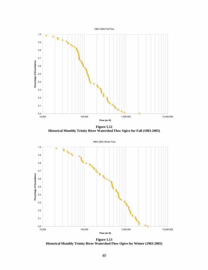
Fall (1,390,620 ; 2,082,474) 68% Confidence bounds denoted by ( ) The recommended frequencies at which these flows might occur can be developed through an investigation of the monthly historical flow frequencies during each season, such as those depicted in Figures 5.10-5.13 for the Trinity watershed. The resultant flow matrix for a given species can thus be presented as shown in Table 5.5.

Table 5.5 Example Flow Matrix for Trinity River Watershed for Atlantic Rangia (2-10 psu)

Species/Season Spring Summer Fall

1,172,671 & 1,766,67412% & 3%

(815,560 ; 2,940,011) (660,810 ; 2,214,891) (1,390,620 ; 2,082,474)42% - 3% 19% - 0% 4% - 0%

Atlantic/Brown Rangia(2-10 psu)

68% Confidence bounds denoted by () Based on the methodology utilized, the resultant matrix can be interpreted such that as long as X-ac-ft. occurs in one month the desired area will be obtained Y% of the time during the given season over the period of record (or analysis period), with an uncertainty that ranges from M-ac-ft that occurs N% of the time to R-ac-ft that occurs S% of the time. In fact, these decisions applied for each identified species under analysis in this study would yield the flow matrices for the Trinity and San Jacinto Rivers presented in Table 5.6 and 5.7 below, respectively. As noted previously, the analyses of historical salinity areas and the resultant relations to monthly flow are provided for each identified species in Appendix B. The associated analyses investigating historical frequencies of occurrence for organism salinity zone areas and their relation to flows for each species are presented in Appendix E. The historical monthly flow ogives for the Trinity and San Jacinto watersheds for each season (as defined herein) and the data upon which they are based are provided in Appendix F.

39

1983~2005 Spring Flow

0.0

0.1

0.2

0.3

0.4

0.5

0.6

0.7

0.8

0.9

1.0

10,000 100,000 1,000,000 10,000,000

Flow (ac-ft)

Perc

enta

ge o

f Exc

eeda

nce

Figure 5.10

Historical Monthly Trinity River Watershed Flow Ogive for Spring (1983-2005)

1983~2005 Summer Flow

0.0

0.1

0.2

0.3

0.4

0.5

0.6

0.7

0.8

0.9

1.0

10,000 100,000 1,000,000 10,000,000

Flow (ac-ft)

Perc

enta

ge o

f Exc

eeda

nce

Figure 5.11

Historical Monthly Trinity River Watershed Flow Ogive for Summer (1983-2005)

40

1983~2005 Fall Flow

0.0

0.1

0.2

0.3

0.4

0.5

0.6

0.7

0.8

0.9

1.0

10,000 100,000 1,000,000 10,000,000

Flow (ac-ft)

Perc

enta

ge o

f Exc

eeda

nce

Figure 5.12

Historical Monthly Trinity River Watershed Flow Ogive for Fall (1983-2005)

1983~2005 Winter Flow

0.0

0.1

0.2

0.3

0.4

0.5

0.6

0.7

0.8

0.9

1.0

10,000 100,000 1,000,000 10,000,000

Flow (ac-ft)

Perc

enta

ge o

f Exc

eeda

nce

Figure 5.13

Historical Monthly Trinity River Watershed Flow Ogive for Winter (1983-2005)

41

Table 5.6 Example Preliminary Flow Matrix for the Trinity River Basin

Species/Season Spring Summer Fall Winter

1,876,390 & 3,507,490 1,885,9506% & 1% 2%

(1,233,252 ; 3,708,904) (1,455,574 ; 2,214,891)(29% ; 0%) (6% ; 0%)

1,172,671 & 1,766,67412% & 3%

(815,560 ; 2,940,011) (660,810 ; 2,214,891) (1,390,620 ; 2,082,474)(42% ; 3%) (19% ; 0%) (4% ; 0%)

(1,093,669 ; 2,771,399) (1,103,861 ; 2,224,153)(35% ; 4%) (28% ; 4%)

1,579,937 & 3,322,520 1,408,556 & 2,971,34614% & 2% 13% & 1%

(928,355 ; 3,708,904) (858,080 ; 3,343,791)(41% ; 0%) (39% ; 0%)

(12,216 ; 47,738) (17,867 ; 26,428)(100% ; 99%) (100% ; 95%)

(12,216 ; 103,654) (17,867 ; 59,296)(100% ; 77%) (100% ; 81%)

(245,386 ; 1,711,069) (63,566 ; 2,082,474)(47% ; 5%) (40% ; 2%)

Mantis Shrimp(>25 psu)

Pinfish(>25 psu)

Oyster Indicators

American Oyster(10-20 psu)

Habitat Indicators

High Flow-Low Salinity Indicators

Low Flow-High Salinity Indicators

Gulf Menhaden(5-15 psu for common

occurrence)

Atlantic Rangia(2-10 psu for larval

survival)

Wild celery(<5 psu for

establishment)

Blue Catfish(<10 psu in single

freshet during seasons)

Red text denotes substitution of historical minimum flow Green text denotes substitution of historical maximum flow.

42

Table 5.7 Example Preliminary Flow Matrix for the San Jacinto River Basin

Species/Season Spring Summer Fall Winter

(320,292 ; 799,144) (800,831 ; 1,501,736)(35% ; 3%) (3% ; 0%)

697,891 & 1,419,1278% & 0.2%

(235,001 ; 815,135) (321,390 ; 1,501,736) (967,728 ; 1,384,362)(45% ; 2%) (17% ; 0%) (3% ; 0%)

('357,277 ; 743,472) (413,582 ; 597,408)(29% ; 5%) (28% ; 10%)

72651738%1%

(245,187 ; 888,311) (320,770 ; 896,815)(44% ; 2%) (35% ; 0%)

(47,693 ; 55,782) (43,260 ; 43,290)(100% ; 92%) (100% ; 100%)

(47,693 ; 108,213) (43,260 ; 91,818)(100% ; 64%) (100% ; 60%)

(186,470 ; 1,335,163) (210,025 ; 1,227,330)(42% ; 0%) (36% ; 2%)

Habitat Indicators

High Flow-Low Salinity Indicators

Low Flow-High Salinity Indicators

Gulf Menhaden(5-15 psu for common

occurrence)

Atlantic Rangia(2-10 psu for larval

survival)

Wild celery(<5 psu for

establishment)

Blue Catfish(<10 psu in single

freshet during seasons)

Oyster Indicators

American Oyster(10-20 psu)

Mantis Shrimp(>25 psu)

Pinfish(>25 psu)

Red text denotes substitution of historical minimum flow Green text denotes substitution of historical maximum flow.

43

It is anticipated that these resultant flow matrices may now be scrutinized and evaluated by the Trinity-San Jacinto BBEST to assess earlier decisions, such as the utility of the selection of the maximum area as the maintenance criterion, the seasonality components, whether the minimum confidence bound or the prediction from the mean might be utilized as a flow recommendation for a given season, the characterization of the high-flow indicator organisms via their monthly relation to salinity, and how these results might be interpreted as a flow recommendation…to name a few. It may also be assessed where certain flows are similar in given time periods, such that flows shown as recommended to maintain some frequency of salinity zone area for one organism may also provide the necessary flows for the frequency of salinity zone area for another organism, and thus condensing of the flow matrix could be possible. As seen from Tables 5.6 and 5.7, there remain several topics to be considered by the BBEST, specifically as to the effect such decisions have upon the subsequent application of the methodology and its derived results. For vallisneria, an organism where it has now been hypothesized that a more improved relation might be developed to seasonal freshets (due to the step-function nature of the relation to its preferred salinity zone area to monthly flows), the selection of the maximum salinity zone area for a maintenance condition is found to unsuccessfully yield a related monthly flow amount for the Trinity nor San Jacinto watersheds during the fall. As can be seen in Figure 5.14 for fall monthly flows from the Trinity Watershed, the regression, even at the historical maximum flow, is unable to yield the historical maximum salinity zone area. This is specifically an artifact of the least-squares fitting of a regression through these data as they are represented and the identification of the historical maximum as the target value to be maintained. Similar situations arise for mantis shrimp and pinfish, although for these organisms (as can be seen in Appendix E) the utilization of an alternative regression form yielding a slightly lower explained variance allows for the identification of a functional monthly flow related to the identified historical maximum salinity zone area.

44

Least Squares Fit to Non-Weighted Quadratic

0

200

400

600

800

1,000

1,200

1,400

1,600

0 200,000 400,000 600,000 800,000 1,000,000 1,200,000 1,400,000 1,600,000

Flow Magnitude (ac-ft/month)

Are

a (h

ecta

res)

Raw DataQuad RegressionLower PIUpper PI

Figure 5.14

Historical Relation between Salinity Zone Area for Vallisneria and Trinity Watershed Monthly Flow - Fall

45

6.0 Conclusions As stated at the outset of this document, organisms have adapted over time to succeed within these estuarine systems’ variable salinity conditions, and it is the characterization of the range and frequency of these conditions which has been identified by the Trinity-San Jacinto BBEST as one critical factor to the maintenance of the ecological health of Galveston Bay’s estuarine environment. This project report describes work performed under a scope of work developed by the Trinity-San Jacinto BBEST to be used in part to support the development of recommended flow quantities and a flow regime supportive of a sound ecological environment for the Galveston Bay system. Through a comparative analysis of statistical regressions on observed data and model results from the TxBLEND hydrodynamic salinity model for Galveston Bay, this study determined that as while the regressions and the TxBLEND model appear to both perform statistically similarly. It was thus determined, through coordination with the TWDB and several SAC members, that the TxBLEND model would prove beneficial for use by the Trinity-San Jacinto BBEST as it would at least allow for specific analyses in external areas of the bay (although it has not been validated in such locations) and could potentially allow for future evaluations of alternative scenarios. Thus the TxBLEND model has been applied to the Galveston Bay system to characterize historical spatial and temporal salinity conditions in Galveston Bay. Through a collaborative process involving staff from TPWD, invited biological experts, SAC members, and members of the Trinity-San Jacinto BBEST a list of selected species has been identified as appropriate biological indicators representative of the ecological characteristics of Galveston Bay. Along with this species list associated salinity ranges and specified regions in the bay from which to assess these ranges has been identified. Utilizing this information, the TxBLEND model results for Galveston Bay from 1983-2005 have been evaluated, and a methodology presented to develop a flow regime recommendation. This methodology investigates the historical frequencies of occurrence for given salinity ranges, spatially translated as areas within the specified regions that are predicted to be within this salinity zone. It is the historical assessment of these salinity zone areas, and their associated relations to flow, that represents the core of the methodology. Incorporated within this methodology are three decision points (DP’s) upon which the BBEST might scrutinize the historical data to arrive at a flow recommendation:

1. What is the associated seasonality of the species to be analyzed, if any, and to what flow timestep should that be related?

2. What frequency of salinity zone area must be maintained? 3. What statistical confidence to apply for the assessment of the relation between

salinity zone area and flow?

46

As discussed within Section 5, each of these decision points, which may be made by the BBEST per individual organism or as blanket decisions for all organisms under analysis, are critical to the resultant flow matrices. It is hypothesized that the identified high-flow species’ salinity zones may be better assessed through an investigation of their relations to longer-term, seasonal pulses (i.e. freshets). The flow matrices could then be assessed to determine where components of these flow matrices might be condensed. It is these flow matrices which may then be utilized as a basis for freshwater inflow recommendations, as they have been developed to represent a wide range of representative indicator organisms’ preferred salinity ranges for various regions of the bay. The flow matrices are based upon the concept of maintaining the maximum area of the indicator organisms at their historical frequency of occurrence, utilizing the best available tools to determine the flows necessary to produce these salinity ranges and acknowledging the uncertainty associated with these relations. This methodology asserts that the “maintenance” of the ecological health of a system is more scientifically defensible when coupled to the biology in such a way that it can be supported by actual data. This is accomplished through the assessment of the historic flow regime and associated historic salinity regime, and the salinity ranges of organisms identified as representative for Galveston Bay. Ultimately it is through these applied methods a more defensible flow recommendation may be made. Indeed, the fundamental question posited via this method that the BBEST must consider is “how much change in salinity area can the bay tolerate?” Through the use of this methodology it is proposed that the BBEST might consider how much change in the historic frequency of occurrence of the salinity zones’ areas is considered “too much”, considering the latent uncertainty shown to exist from the available data and methods utilized to characterize the system. The relations presented in Appendix D present the context in which historical frequencies of the identified salinity zone areas have occurred, with the latent uncertainty about these areas’ relations to flow depicted. It is proffered that such an assessment, performed in an ecologic context, is a more scientifically defensible approach to the development of a flow regime recommendation for the Galveston Bay system.

47

7.0 References Cole, TM, and SA Wells. 2002. CE-QUAL-W2: A two-dimensional, laterally averaged,

hydrodynamic and water quality model, version 3.1: user manual. Instruction report EL-02-1. U.S. Army Corps of Engineers, Washington DC, August 2002.

Lee, W., D. Buzan, P. Eldridge, and W. Pulich, Jr.,. Freshwater Inflow Recommendation for the Trinity – San Jacinto Estuary of Texas. Texas Parks and Wildlife, February 2001.

Leggett, R. W., and Williams, L.R. 1981. “A Reliability Index for Models,” Ecological Modelling, 13:303-312.

Longley, W.L. 1994. Freshwater inflows to Texas bays and estuaries: ecological relationships and methods for determination of needs. Texas Water Development Board and Texas Parks and Wildlife Department, Austin. 386 pp. Matsumoto, J., 1992. Users Manual for The Texas Water Development Board’s Circulation and Salinity Model: TxBLEND. Texas Water Development Board.

Matsumoto, J., Users Maual for The Texas Water Development Board’s Circulation and Salinity Model: TxBLEND. Texas Water Development Board. September, 1992.

Matsumoto, J., Effects of Structures and Practices on the Circulation and Salinity Patterns of Galveston Bay, Texas. Texas Water Development Board. February, 2005.

Monismith, S.G., “Letter to TWDB regarding the suitability of the hydrodynamics/transport model (code) TxBLEND” January, 29,2005.

Ward, G. in association with Espey, Padden Consultants, Inc., Brown & Root, Inc. and Freese & Nichols, Inc., Technical Basis for Establishing Freshwater Inflow Requirements for Galveston Bay, Prepared for the Trinity River Authority, Tarrant Regional Water District and the City of Houston. November 1999.

Wlosinski, JH. 1984. Evaluation techniques for CE-QUAL-R1 – a one-dimensional

reservoir water quality model. Miscellaneous Paper E-84-1. U.S. Army Corps of Engineers Waterways Experiment Station, Vicksburg, MS.