1

Techniques of Precipitation Analysis and Prediction for High-resolution Precipitation Nowcasts

The Japan Meteorological Agency*

Abstract

High-resolution Precipitation Nowcasts (HRPNs) – a type of close-up high-precision precipitation

analysis and prediction – were introduced in 2014 primarily to support the observation and prediction

of localized heavy rain. As such rainfall events caused by cumulonimbus clouds are generally

short-term phenomena, HRPNs involve both extrapolation and spatially three-dimensional forecasting

for heavy rain areas. These techniques enable practical prediction of rapidly developing heavy rainfall

events.

This paper describes the techniques used for precipitation analysis and prediction in HRPN

generation as described in the Japan Meteorological Agency’s Weather Forecast Training Textbook (in

Japanese).

1. Introduction

The Japan Meteorological Agency (JMA) works to enhance capacity for the observation and

prediction of localized heavy rainfall using high-precision radar observation data. The Agency

upgraded the data processing systems of all its radar sites in Japan and installed its High-resolution

Precipitation Prediction System in FY 2012 and 2013. These enhancements helped JMA to develop

High-resolution Precipitation Nowcasts, (HRPNs), which support close-up high-precision

precipitation analysis and prediction. HRPNs involve the use of an X-band multi-parameter radar

observation system (referred to here simply as X-band) called XRAIN operated by Japan’s Ministry of

Land, Infrastructure, Transport and Tourism (MLIT).

HRPNs, as the name suggests, are precipitation nowcasting products with the grid point interval

shortened from the conventional 1 km to 250 m for higher resolution. Conventional precipitation

nowcasts are generated using only observation data from JMA’s C-band Doppler Radar (referred to

here simply as C-band), while HRPNs involve the use of varied observation radar data such as C-band

and XRAIN in addition to the advanced application of observation data from the Automated

Meteorological Data Acquisition System (AMeDAS) as well as upper-air radiosonde and wind

profiler observation information.

JMA has developed two key techniques for the generation of HRPNs: 1) a spatially

* Corresponding author: Seiichiro Kigawa

2

three-dimensional prediction approach for heavy rainfall domains, including prediction for heavy

rainfall areas where no heavy rainfall is initially observed; and 2) an approach incorporating a

relatively long temporal scale and a large spatial scale (for phenomena such as stationary linear heavy

rainfall and rain generated by typhoons) to improve forecast accuracy for rain events.

The advanced application of these observation data and techniques is based on concepts differing

from those of conventional precipitation nowcasts. For instance, the data processing functions used for

HRPN analysis and prediction were enhanced for optimal performance in the analysis and prediction

of ground-level precipitation amounts and intensity. In other development for HRPN prediction

techniques, data processing functions were innovated using methods including 1) a kinetic prediction

approach in which phenomenon movement trends are extrapolated, and 2) a dynamical estimation

approach for the prediction of short-term and significantly developing rain phenomena.

Thus, HRPNs are a new precipitation nowcasting product based on the comprehensive use of

observation data from various sources and the application of some of the world’s most advanced

techniques.

2. Algorithms

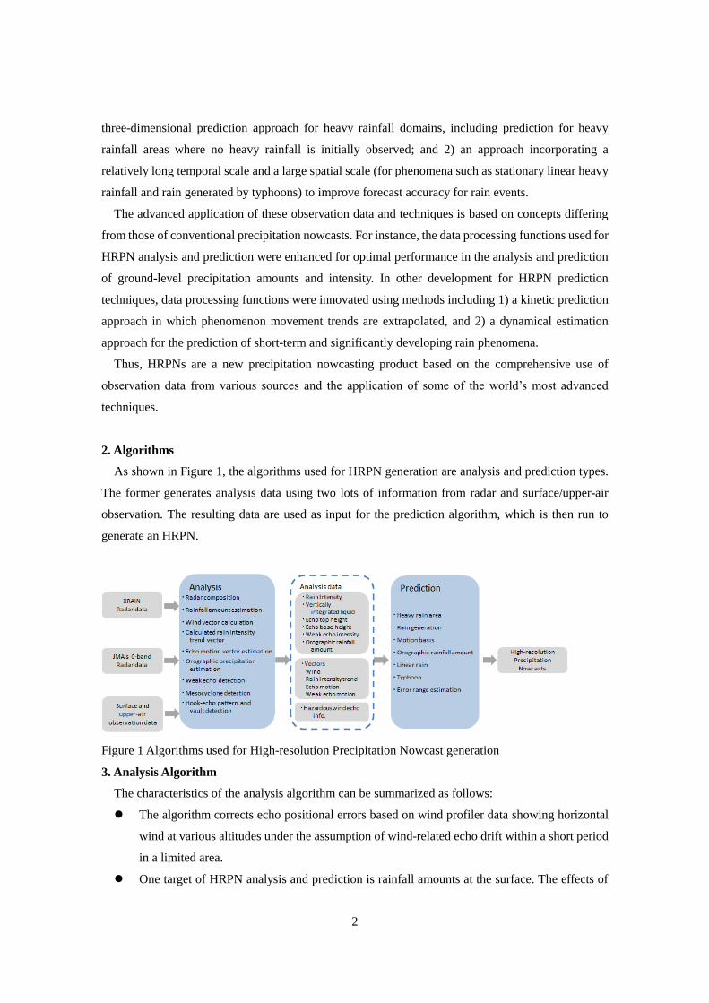
As shown in Figure 1, the algorithms used for HRPN generation are analysis and prediction types.

The former generates analysis data using two lots of information from radar and surface/upper-air

observation. The resulting data are used as input for the prediction algorithm, which is then run to

generate an HRPN.

Figure 1 Algorithms used for High-resolution Precipitation Nowcast generation

3. Analysis Algorithm

The characteristics of the analysis algorithm can be summarized as follows:

The algorithm corrects echo positional errors based on wind profiler data showing horizontal

wind at various altitudes under the assumption of wind-related echo drift within a short period

in a limited area.

One target of HRPN analysis and prediction is rainfall amounts at the surface. The effects of

3

horizontal raindrop drift are corrected based on the calculation of such drift during descent

from an altitude of around 1 to 2 km, which is the height used for radar-based rain intensity

estimation.

Radar clutter is detected by analyzing a vertical radar beam pattern based on a clutter

phenomenon by which the intensity of reflected radar beams rapidly decreases with height due

to sources of clutter on or near the ground.

The altitude and thickness of radar’s bright bands are estimated from the size and shape of the

ring-shaped echo observed at the maximum radar scan elevation, vertical speed as observed

using wind profilers, and surface temperature from AMeDAS data.

The processes of radar composition are as follows:

In the C-band, rain intensity at a specific height for each radar is estimated using a method

for linear interpolation between data of two scan elevation angles. A nationwide radar

composition of rain intensity analysis is then calculated using the weighted average

method, by which radar intensity for every radar is averaged with different weights.

In the X-band, a nationwide radar composition is calculated using the maximum method

because the weighted average method may result in underestimation of rain intensity if

rain-related radio wave attenuation is not estimated accurately.

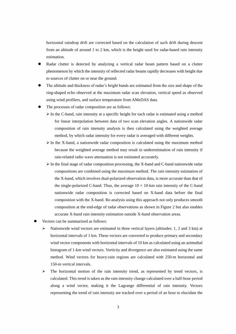
In the final stage of radar composition processing, the X-band and C-band nationwide radar

compositions are combined using the maximum method. The rain intensity estimation of

the X-band, which involves dual-polarized observation data, is more accurate than that of

the single-polarized C-band. Thus, the average 10 × 10-km rain intensity of the C-band

nationwide radar composition is corrected based on X-band data before the final

composition with the X-band. Re-analysis using this approach not only produces smooth

composition at the end-edge of radar observations as shown in Figure 2 but also enables

accurate X-band rain intensity estimation outside X-band observation areas.

Vectors can be summarized as follows:

Nationwide wind vectors are estimated in three vertical layers (altitudes: 1, 2 and 3 km) at

horizontal intervals of 1 km. These vectors are converted to produce primary and secondary

wind vector components with horizontal intervals of 10 km as calculated using an azimuthal

histogram of 1-km wind vectors. Vorticity and divergence are also estimated using the same

method. Wind vectors for heavy-rain regions are calculated with 250-m horizontal and

150-m vertical intervals.

The horizontal motion of the rain intensity trend, as represented by trend vectors, is

calculated. This trend is taken as the rain intensity change calculated over a half-hour period

along a wind vector, making it the Lagrange differential of rain intensity. Vectors

representing the trend of rain intensity are tracked over a period of an hour to elucidate the

4

longer-term scale change in an area of rain.

A multi-scale motion detection technique corresponding to the conventional method of echo

motion vector calculation in Precipitation Nowcasts is adopted to highlight temporally and

spatially varying scales of motion for echo motion vector estimation.

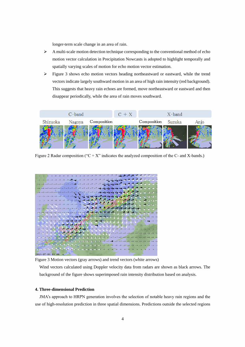
Figure 3 shows echo motion vectors heading northeastward or eastward, while the trend

vectors indicate largely southward motion in an area of high rain intensity (red background).

This suggests that heavy rain echoes are formed, move northeastward or eastward and then

disappear periodically, while the area of rain moves southward.

Figure 2 Radar composition (“C + X” indicates the analyzed composition of the C- and X-bands.)

Figure 3 Motion vectors (gray arrows) and trend vectors (white arrows)

Wind vectors calculated using Doppler velocity data from radars are shown as black arrows. The

background of the figure shows superimposed rain intensity distribution based on analysis.

4. Three-dimensional Prediction

JMA’s approach to HRPN generation involves the selection of notable heavy rain regions and the

use of high-resolution prediction in three spatial dimensions. Predictions outside the selected regions

5

are generated using a longer time step and fewer vertical calculations based on various types of

two-dimensional information converted from the three-dimensional distribution of rain. This enables

high-resolution, high-quality prediction with guaranteed timeliness for nowcasting products.

5. High-resolution Three-dimensional Prediction

High-resolution Three-dimensional Prediction involves extrapolation of precipitation analysis and

prediction obtained from the Vertically One-dimensional Convection Model (VOCM). Analysis

extrapolation is used to predict three-dimensional distribution of water content based on the

integration of HRPN analysis with one-minute time steps using the time integration of the

semi-Lagrangian method. The time integration is divided into two types: (1) that of water content

exclusively in the vertical direction in proportion to the terminal velocity estimated on the basis of

water content, and (2) that in all directions based on three-dimensional wind vectors calculated from

radar Doppler velocity data. The results of calculation for these values are combined using the

maximum method to generate predictions. In this way, it is possible to predict the movement, rotation,

extent, growth and decline of rain areas because the water content of (2) is multiplied by a factor

relative to the trend of growth/decline in the rain area or rainfall as predicted using the VOCM. This

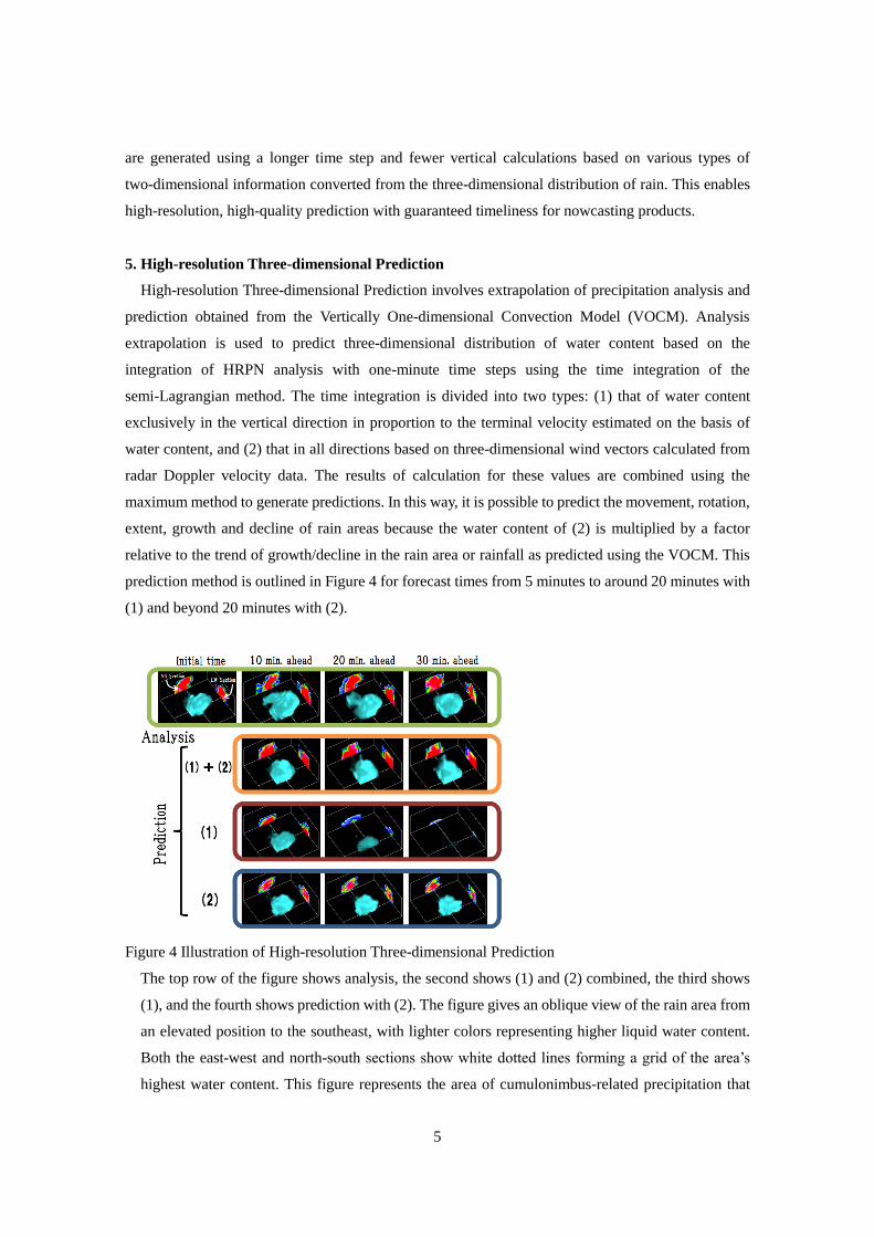
prediction method is outlined in Figure 4 for forecast times from 5 minutes to around 20 minutes with

(1) and beyond 20 minutes with (2).

Figure 4 Illustration of High-resolution Three-dimensional Prediction

The top row of the figure shows analysis, the second shows (1) and (2) combined, the third shows

(1), and the fourth shows prediction with (2). The figure gives an oblique view of the rain area from

an elevated position to the southeast, with lighter colors representing higher liquid water content.

Both the east-west and north-south sections show white dotted lines forming a grid of the area’s

highest water content. This figure represents the area of cumulonimbus-related precipitation that

6

brought hail to the Mitaka area of Tokyo with an initial time of 14:30 on June 24 2014. The

awning-shaped echo structures (called overhangs) in the figure suggest the presence of strong

updrafts. It should be noted that practical prediction processing involves a supply of water content

from (2) to (1), while the figure for (1) shows the results of calculation with zero supply for simple

representation of how rain falls.

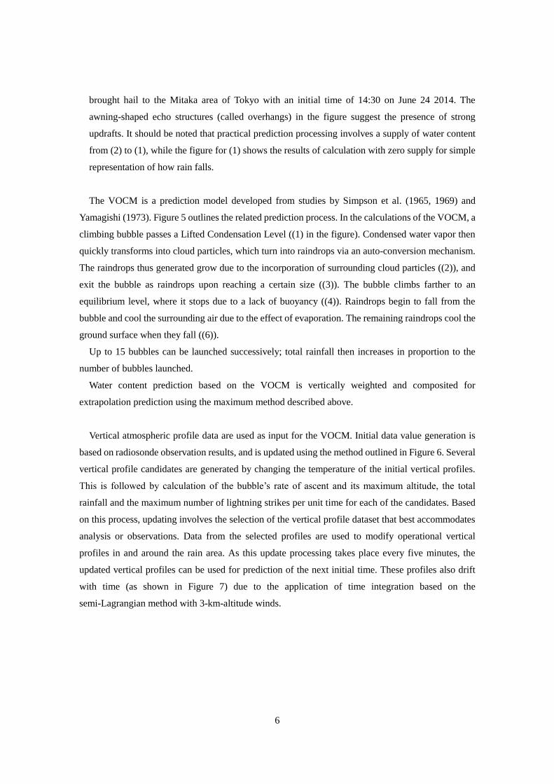
The VOCM is a prediction model developed from studies by Simpson et al. (1965, 1969) and

Yamagishi (1973). Figure 5 outlines the related prediction process. In the calculations of the VOCM, a

climbing bubble passes a Lifted Condensation Level ((1) in the figure). Condensed water vapor then

quickly transforms into cloud particles, which turn into raindrops via an auto-conversion mechanism.

The raindrops thus generated grow due to the incorporation of surrounding cloud particles ((2)), and

exit the bubble as raindrops upon reaching a certain size ((3)). The bubble climbs farther to an

equilibrium level, where it stops due to a lack of buoyancy ((4)). Raindrops begin to fall from the

bubble and cool the surrounding air due to the effect of evaporation. The remaining raindrops cool the

ground surface when they fall ((6)).

Up to 15 bubbles can be launched successively; total rainfall then increases in proportion to the

number of bubbles launched.

Water content prediction based on the VOCM is vertically weighted and composited for

extrapolation prediction using the maximum method described above.

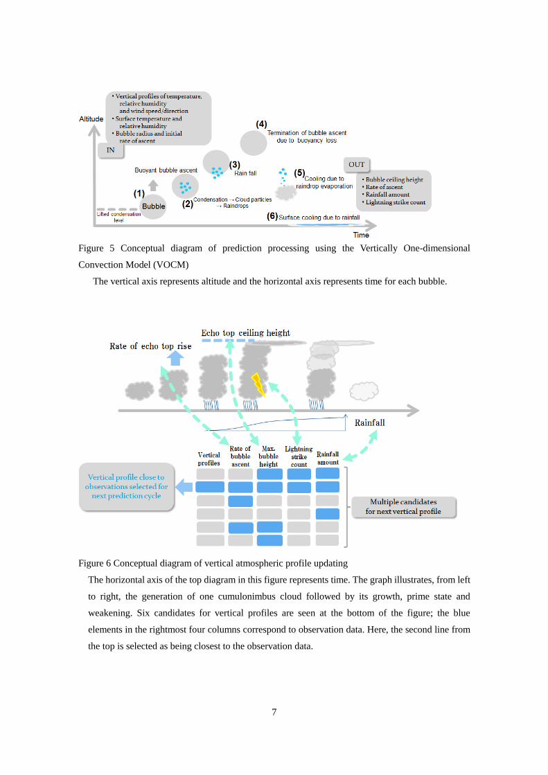
Vertical atmospheric profile data are used as input for the VOCM. Initial data value generation is

based on radiosonde observation results, and is updated using the method outlined in Figure 6. Several

vertical profile candidates are generated by changing the temperature of the initial vertical profiles.

This is followed by calculation of the bubble’s rate of ascent and its maximum altitude, the total

rainfall and the maximum number of lightning strikes per unit time for each of the candidates. Based

on this process, updating involves the selection of the vertical profile dataset that best accommodates

analysis or observations. Data from the selected profiles are used to modify operational vertical

profiles in and around the rain area. As this update processing takes place every five minutes, the

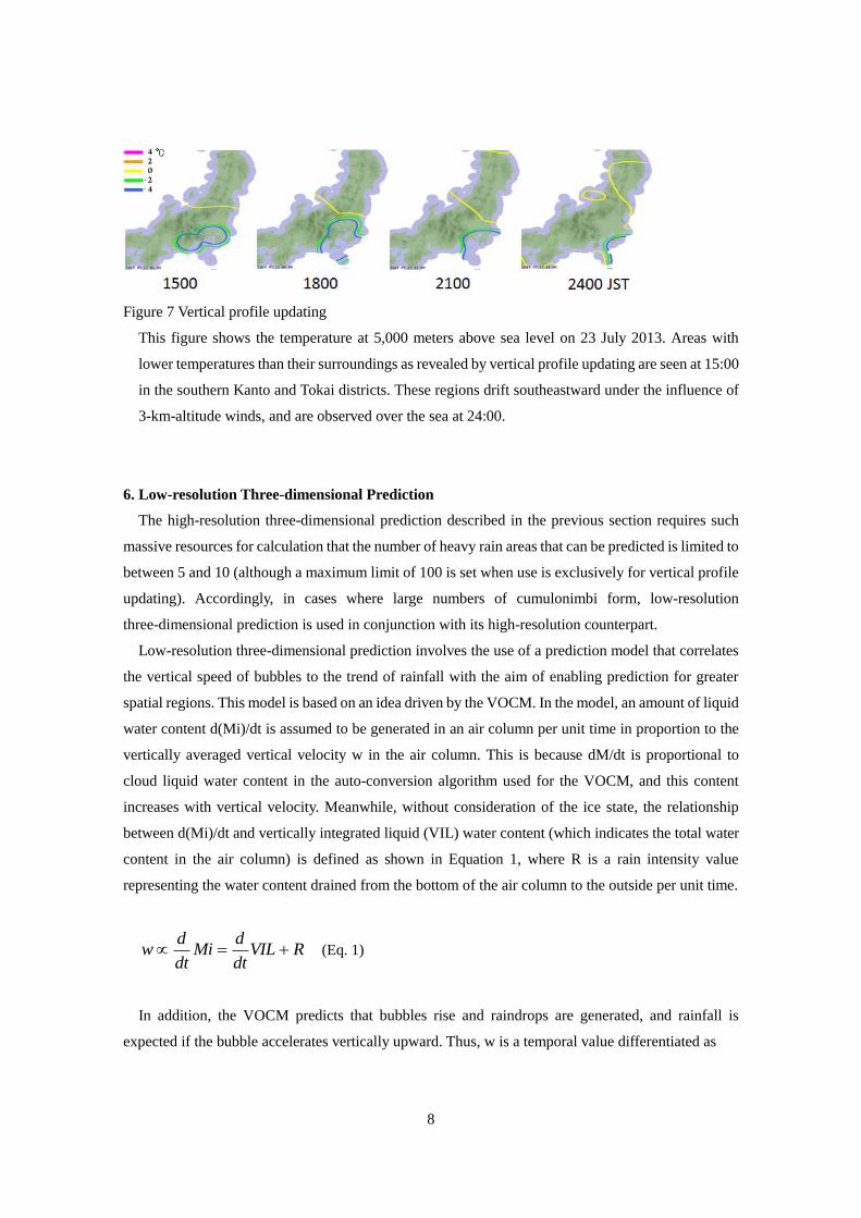
updated vertical profiles can be used for prediction of the next initial time. These profiles also drift

with time (as shown in Figure 7) due to the application of time integration based on the

semi-Lagrangian method with 3-km-altitude winds.

7

Figure 5 Conceptual diagram of prediction processing using the Vertically One-dimensional

Convection Model (VOCM)

The vertical axis represents altitude and the horizontal axis represents time for each bubble.

Figure 6 Conceptual diagram of vertical atmospheric profile updating

The horizontal axis of the top diagram in this figure represents time. The graph illustrates, from left

to right, the generation of one cumulonimbus cloud followed by its growth, prime state and

weakening. Six candidates for vertical profiles are seen at the bottom of the figure; the blue

elements in the rightmost four columns correspond to observation data. Here, the second line from

the top is selected as being closest to the observation data.

8

Figure 7 Vertical profile updating

This figure shows the temperature at 5,000 meters above sea level on 23 July 2013. Areas with

lower temperatures than their surroundings as revealed by vertical profile updating are seen at 15:00

in the southern Kanto and Tokai districts. These regions drift southeastward under the influence of

3-km-altitude winds, and are observed over the sea at 24:00.

6. Low-resolution Three-dimensional Prediction

The high-resolution three-dimensional prediction described in the previous section requires such

massive resources for calculation that the number of heavy rain areas that can be predicted is limited to

between 5 and 10 (although a maximum limit of 100 is set when use is exclusively for vertical profile

updating). Accordingly, in cases where large numbers of cumulonimbi form, low-resolution

three-dimensional prediction is used in conjunction with its high-resolution counterpart.

Low-resolution three-dimensional prediction involves the use of a prediction model that correlates

the vertical speed of bubbles to the trend of rainfall with the aim of enabling prediction for greater

spatial regions. This model is based on an idea driven by the VOCM. In the model, an amount of liquid

water content d(Mi)/dt is assumed to be generated in an air column per unit time in proportion to the

vertically averaged vertical velocity w in the air column. This is because dM/dt is proportional to

cloud liquid water content in the auto-conversion algorithm used for the VOCM, and this content

increases with vertical velocity. Meanwhile, without consideration of the ice state, the relationship

between d(Mi)/dt and vertically integrated liquid (VIL) water content (which indicates the total water

content in the air column) is defined as shown in Equation 1, where R is a rain intensity value

representing the water content drained from the bottom of the air column to the outside per unit time.

RVILdt

dMi

dt

dw (Eq. 1)

In addition, the VOCM predicts that bubbles rise and raindrops are generated, and rainfall is

expected if the bubble accelerates vertically upward. Thus, w is a temporal value differentiated as

9

Rdt

dVIL

dt

dw

dt

d

2

2

(Eq. 2)

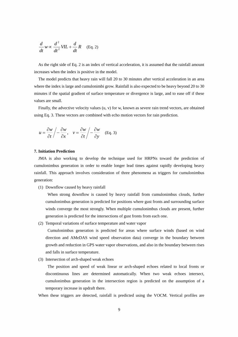
As the right side of Eq. 2 is an index of vertical acceleration, it is assumed that the rainfall amount

increases when the index is positive in the model.

The model predicts that heavy rain will fall 20 to 30 minutes after vertical acceleration in an area

where the index is large and cumulonimbi grow. Rainfall is also expected to be heavy beyond 20 to 30

minutes if the spatial gradient of surface temperature or divergence is large, and to ease off if these

values are small.

Finally, the advective velocity values (u, v) for w, known as severe rain trend vectors, are obtained

using Eq. 3. These vectors are combined with echo motion vectors for rain prediction.

y

w

t

wv

x

w

t

wu

, (Eq. 3)

7. Initiation Prediction

JMA is also working to develop the technique used for HRPNs toward the prediction of

cumulonimbus generation in order to enable longer lead times against rapidly developing heavy

rainfall. This approach involves consideration of three phenomena as triggers for cumulonimbus

generation:

(1) Downflow caused by heavy rainfall

When strong downflow is caused by heavy rainfall from cumulonimbus clouds, further

cumulonimbus generation is predicted for positions where gust fronts and surrounding surface

winds converge the most strongly. When multiple cumulonimbus clouds are present, further

generation is predicted for the intersections of gust fronts from each one.

(2) Temporal variations of surface temperature and water vapor

Cumulonimbus generation is predicted for areas where surface winds (based on wind

direction and AMeDAS wind speed observation data) converge in the boundary between

growth and reduction in GPS water vapor observations, and also in the boundary between rises

and falls in surface temperature.

(3) Intersection of arch-shaped weak echoes

The position and speed of weak linear or arch-shaped echoes related to local fronts or

discontinuous lines are determined automatically. When two weak echoes intersect,

cumulonimbus generation in the intersection region is predicted on the assumption of a

temporary increase in updraft there.

When these triggers are detected, rainfall is predicted using the VOCM. Vertical profiles are

10

adjusted directionally for stability when no new cumulonimbus clouds actually appear despite the

appearance of triggers, when aerial conditions are unstable, and when cumulonimbus generation is

predicted.

Due to the presence of fewer AMeDAS observation stations on islands/mountains and difficulties in

detecting weak echoes in mountainous areas, generation prediction based on the above techniques

results in a probability of detection (POD) below 10%. Accordingly, further improvement is needed.

8. Error Range Estimation

HRPN distribution data consist of information on five-minute integral rainfall amounts and rain

intensity. The data contain different types of information on analysis/prediction uncertainty.

The integral rainfall amount data generally applied to quantitative forecasting contain an estimated

error range ε. With P defined as the hourly rainfall amount forecast and O as the amount observed,

the probability that P – O will be between –2ε and +ε is about 70%. As the hourly rainfall amount

forecast error (P – O) can actually be determined after an hour, ε represents a prediction of the error

range included in the rainfall amount forecast.

Meanwhile, rain intensity data contain information on possible sources of error in rain intensity

analysis, such as clutter, bright-band, upper-air echo or hail, as an alert to increased uncertainty on the

assumption of visual application.

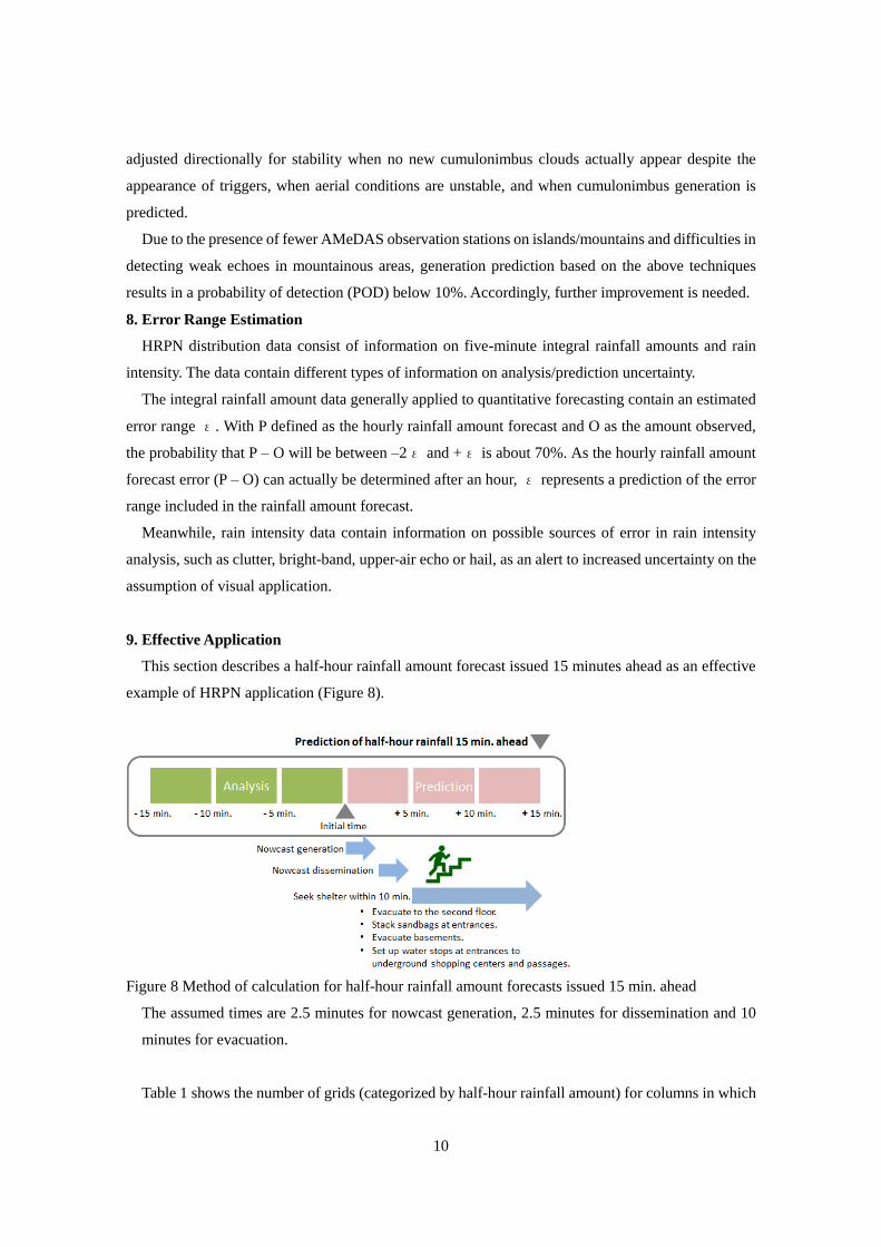
9. Effective Application

This section describes a half-hour rainfall amount forecast issued 15 minutes ahead as an effective

example of HRPN application (Figure 8).

Figure 8 Method of calculation for half-hour rainfall amount forecasts issued 15 min. ahead

The assumed times are 2.5 minutes for nowcast generation, 2.5 minutes for dissemination and 10

minutes for evacuation.

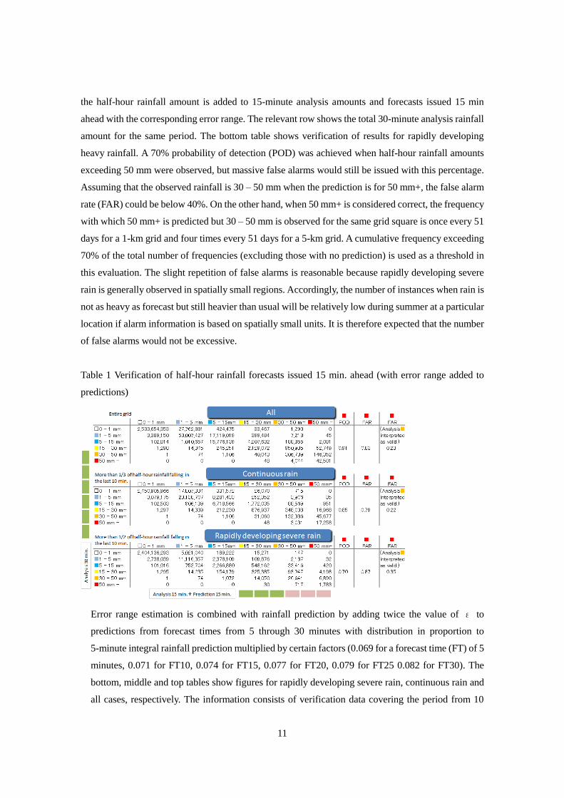
Table 1 shows the number of grids (categorized by half-hour rainfall amount) for columns in which

11

the half-hour rainfall amount is added to 15-minute analysis amounts and forecasts issued 15 min

ahead with the corresponding error range. The relevant row shows the total 30-minute analysis rainfall

amount for the same period. The bottom table shows verification of results for rapidly developing

heavy rainfall. A 70% probability of detection (POD) was achieved when half-hour rainfall amounts

exceeding 50 mm were observed, but massive false alarms would still be issued with this percentage.

Assuming that the observed rainfall is 30 – 50 mm when the prediction is for 50 mm+, the false alarm

rate (FAR) could be below 40%. On the other hand, when 50 mm+ is considered correct, the frequency

with which 50 mm+ is predicted but 30 – 50 mm is observed for the same grid square is once every 51

days for a 1-km grid and four times every 51 days for a 5-km grid. A cumulative frequency exceeding

70% of the total number of frequencies (excluding those with no prediction) is used as a threshold in

this evaluation. The slight repetition of false alarms is reasonable because rapidly developing severe

rain is generally observed in spatially small regions. Accordingly, the number of instances when rain is

not as heavy as forecast but still heavier than usual will be relatively low during summer at a particular

location if alarm information is based on spatially small units. It is therefore expected that the number

of false alarms would not be excessive.

Table 1 Verification of half-hour rainfall forecasts issued 15 min. ahead (with error range added to

predictions)

Error range estimation is combined with rainfall prediction by adding twice the value of ε to

predictions from forecast times from 5 through 30 minutes with distribution in proportion to

5-minute integral rainfall prediction multiplied by certain factors (0.069 for a forecast time (FT) of 5

minutes, 0.071 for FT10, 0.074 for FT15, 0.077 for FT20, 0.079 for FT25 0.082 for FT30). The

bottom, middle and top tables show figures for rapidly developing severe rain, continuous rain and

all cases, respectively. The information consists of verification data covering the period from 10

12

July 2014 through 31 August 2014 at 10-min. intervals over land based on 1-km grid data converted

from a 250-m grid via simple averaging.

As described above, it is considered feasible to issue half-hour rainfall amount forecasts 15 minutes

ahead with the smallest unit of information condensed to a 1-km grid with a high POD and a low false

alarm rate. This allows the practical provision of reliable information with a short lead time.

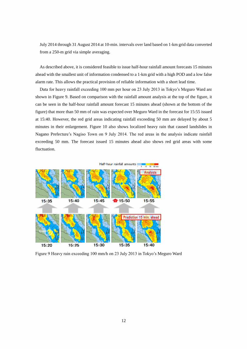
Data for heavy rainfall exceeding 100 mm per hour on 23 July 2013 in Tokyo’s Meguro Ward are

shown in Figure 9. Based on comparison with the rainfall amount analysis at the top of the figure, it

can be seen in the half-hour rainfall amount forecast 15 minutes ahead (shown at the bottom of the

figure) that more than 50 mm of rain was expected over Meguro Ward in the forecast for 15:55 issued

at 15:40. However, the red grid areas indicating rainfall exceeding 50 mm are delayed by about 5

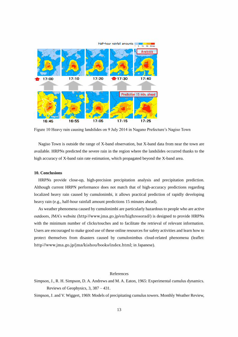
minutes in their enlargement. Figure 10 also shows localized heavy rain that caused landslides in

Nagano Prefecture’s Nagiso Town on 9 July 2014. The red areas in the analysis indicate rainfall

exceeding 50 mm. The forecast issued 15 minutes ahead also shows red grid areas with some

fluctuation.

Figure 9 Heavy rain exceeding 100 mm/h on 23 July 2013 in Tokyo’s Meguro Ward

13

Figure 10 Heavy rain causing landslides on 9 July 2014 in Nagano Prefecture’s Nagiso Town

Nagiso Town is outside the range of X-band observation, but X-band data from near the town are

available. HRPNs predicted the severe rain in the region where the landslides occurred thanks to the

high accuracy of X-band rain rate estimation, which propagated beyond the X-band area.

10. Conclusions

HRPNs provide close-up, high-precision precipitation analysis and precipitation prediction.

Although current HRPN performance does not match that of high-accuracy predictions regarding

localized heavy rain caused by cumulonimbi, it allows practical prediction of rapidly developing

heavy rain (e.g., half-hour rainfall amount predictions 15 minutes ahead).

As weather phenomena caused by cumulonimbi are particularly hazardous to people who are active

outdoors, JMA’s website (http://www.jma.go.jp/en/highresorad/) is designed to provide HRPNs

with the minimum number of clicks/touches and to facilitate the retrieval of relevant information.

Users are encouraged to make good use of these online resources for safety activities and learn how to

protect themselves from disasters caused by cumulonimbus cloud-related phenomena (leaflet:

http://www.jma.go.jp/jma/kishou/books/index.html; in Japanese).

References

Simpson, J., R. H. Simpson, D. A. Andrews and M. A. Eaton, 1965: Experimental cumulus dynamics.

Reviews of Geophysics, 3, 387 – 431.

Simpson, J. and V. Wiggert, 1969: Models of precipitating cumulus towers. Monthly Weather Review,

14

97, 471 – 489.

Yamagishi, Y., 1973: On the characteristics of a One-dimensional Model of Cumulus Convection.

Papers in Meteorology and Geophysics, Vol. 24, No. 1, pp. 79 – 109.