mediatum.ub.tum.demediatum.ub.tum.de/doc/977798/file.pdftechnische universitÄt mÜnchen fakultÄt...
TRANSCRIPT

◦
◦ ◦ ◦
◦ ◦ ◦ ◦
◦ ◦
◦ ◦ ◦
◦ ◦ ◦ ◦
◦ ◦ ◦
TECHNISCHE UNIVERSITÄT MÜNCHEN
FAKULTÄT FÜR INFORMATIK
Lehrstuhl für Effiziente Algorithmen
Counting in the Jacobian of Hyperelliptic CurvesIn the light of genus 2 curves for cryptography
Sandeep Sadanandan
Vollständiger Abdruck der von der Fakultät für Informatik der Technischen UniversitätMünchen zur Erlangung des akademischen Grades eines
Doktors der Naturwissenschaften (Dr. rer. nat.)
genehmigten Dissertation.
Vorsitzender: UNIV.-PROF. DR. GEORG CARLE
Prüfer der Dissertation:
1. UNIV.-PROF. DR. ERNST W. MAYR
2. UNIV.-PROF. DR. HANS-JOACHIM BUNGARTZ
Die Dissertation wurde am 06.05.2010 bei der Technischen Universität München
eingereicht und durch die Fakultät für Informatik am 24.09.2010 angenommen.

ii
Document Classification according to ACM CCS (1998)
Categories and subject descriptors:

Abstract
With the drastic increase in the number and the use of handheld devices, – mobile
phones and smart cards – light weight cryptography has come to the lime light. El-
liptic and Hyperelliptic curve cryptosystems (ECC, HECC) are emerging as the best
solutions for light weight cryptography. Like in any traditional cryptosystem, the size
of the cipher-text space is a significant factor indicating the achievable security level. In
the traditional systems, the size of the group on which the system is defined, defines
the cipher-text space. Unlike the traditional ones, ECC and HECC are defined on the
Jacobian of curves. Gaining knowledge about the size of the Jacobian is not straight-
forward and the computation is inefficient. Since the generic group order counting
methods are incapable of counting in large groups of cryptographic size (2160), special
methods were devised for counting in the Jacobian of hyperelliptic curves, which are
not yet fast enough for practical applications. In this thesis, we are bringing together
the advances in group order counting and the special properties of genus 2 hyperelliptic
curves. The Primorial method for group order counting is applied in a special interval
where the group order is predicted to be. The resulting method provides an improve-
ment factor of Pϕ(P )
, where P is the product of the first p primes and ϕ is Euler’s totient
function. We will see that the value of p varies, depending on the expected size of the
Jacobian. It will also be shown that the factor of improvement becomes larger when the
size of the group gets larger.
iii

iv

Acknowledgment
It would not have been possible to finish this thesis, without the help from many people.
On successful completion of the dissertation I take this opportunity to thank all those
involved directly or indirectly in its accomplishment.
First and foremost, I thank Prof. Dr. Ernst W Mayr for accepting me as a doctoral
candidate to work at the Chair for Efficient Algorithms. He has been very kind to me all
through the 4 years of my doctoral studies. For any kind of academic or non-academic
matters, I could approach him and there was always some solution to my problems.The
discussions with him were invaluable; the discussions and his infinite energy have in-
spired and encouraged me innumerous times during the past few years.
I also thank Dr. Peter Ullrich, who guided me through the first few months of doc-
toral studies. It was he who gave me the initial momentum which helped me continue
my research on the topic of this thesis.
The atmosphere in the institute was always very warm. Hanjo, who could be very
well be called the “Guru” of the chair was there to answer any logistical queries. Ernst
Bayer and the secretaries were more than friendly and helpful whenever I was in need.
Johannes Nowak, Johannes Krugel and Stefan Schmidt were always there for any little
puzzles or riddles or some random proofs/jokes. I thank all of them for being wonder-
ful.
Many thanks to the member of GraduiertenKollege GKAAM and German Research
Foundation (DFG - Deutsche Forschungsgemeinschaft) for the scholarship they pro-
vided me for the initial couple of years.
Last but not the least - family and friends. On this occasion I not only thank them,
but also express my love for all of them. I thank Rajyalakshmi for being there for almost
anything I needed during my doctoral studies. I also thank Suthirtha Saha who helped
me initially with coming to Germany. The list would get too long, if I am to do so. I once
again thank everybody who helped directly or indirectly in the making of this thesis.
Sandeep Sadanandan
München, May 2010
v

vi

IT IS BETTER TO DO THE RIGHT PROBLEM THE WRONG WAY THAN THE
WRONG PROBLEM THE RIGHT WAY.
- RICHARD HAMMING.
vii

viii

Contents
vii
Preface xvii
1 Introduction 1
1.1 Light weight cryptography . . . . . . . . . . . . . . . . . . . . . . . . . . . 2
1.2 Generic algorithms . . . . . . . . . . . . . . . . . . . . . . . . . . . . . . . . 2
1.2.1 Private key systems . . . . . . . . . . . . . . . . . . . . . . . . . . . 3
1.2.2 Public key systems . . . . . . . . . . . . . . . . . . . . . . . . . . . . 3
1.3 Improvement over traditional systems . . . . . . . . . . . . . . . . . . . . . 5
1.3.1 What is this thesis about? . . . . . . . . . . . . . . . . . . . . . . . . 6
1.4 Bird’s view . . . . . . . . . . . . . . . . . . . . . . . . . . . . . . . . . . . . . 6
1.5 A note on notation . . . . . . . . . . . . . . . . . . . . . . . . . . . . . . . . 8
2 Mathematical Background 9
2.1 Cryptographic requirements . . . . . . . . . . . . . . . . . . . . . . . . . . . 9
2.1.1 One way functions . . . . . . . . . . . . . . . . . . . . . . . . . . . . 10
2.1.2 Discrete Logarithm Problem - DLP . . . . . . . . . . . . . . . . . . . 11
2.2 Algebraic geometry . . . . . . . . . . . . . . . . . . . . . . . . . . . . . . . . 12
2.2.1 Affine geometry . . . . . . . . . . . . . . . . . . . . . . . . . . . . . . 12
2.2.2 Projective geometry . . . . . . . . . . . . . . . . . . . . . . . . . . . 13
2.2.3 Affine and projective spaces - relation . . . . . . . . . . . . . . . . . 14
2.2.4 Divisors . . . . . . . . . . . . . . . . . . . . . . . . . . . . . . . . . . 17
2.2.5 Genus of a curve . . . . . . . . . . . . . . . . . . . . . . . . . . . . . 18
2.3 Hyperelliptic curves . . . . . . . . . . . . . . . . . . . . . . . . . . . . . . . 19
2.3.1 Examples . . . . . . . . . . . . . . . . . . . . . . . . . . . . . . . . . 19
2.3.2 Divisors . . . . . . . . . . . . . . . . . . . . . . . . . . . . . . . . . . 22
ix

x CONTENTS
2.3.3 Semi-reduced divisors . . . . . . . . . . . . . . . . . . . . . . . . . . 22
2.3.4 Reduced divisors . . . . . . . . . . . . . . . . . . . . . . . . . . . . . 22
2.3.5 Representations of divisors . . . . . . . . . . . . . . . . . . . . . . . 23
2.4 Jacobian of a curve . . . . . . . . . . . . . . . . . . . . . . . . . . . . . . . . 25
2.4.1 Group operation in Jacobian . . . . . . . . . . . . . . . . . . . . . . 25
2.5 Frobenius endomorphism . . . . . . . . . . . . . . . . . . . . . . . . . . . . 26
2.5.1 Characteristic polynomial . . . . . . . . . . . . . . . . . . . . . . . . 27
2.5.2 Bounds on cardinality - Weil Interval . . . . . . . . . . . . . . . . . 27
2.6 Addition algorithms for divisors . . . . . . . . . . . . . . . . . . . . . . . . 28
2.6.1 Geometrically what is it? . . . . . . . . . . . . . . . . . . . . . . . . 28
2.6.2 Examples . . . . . . . . . . . . . . . . . . . . . . . . . . . . . . . . . 29
2.6.3 Algebraic methods . . . . . . . . . . . . . . . . . . . . . . . . . . . . 29
2.7 ECDLP and HECDLP . . . . . . . . . . . . . . . . . . . . . . . . . . . . . . . 33
2.7.1 Elliptic Curve Discrete Logarithm Problem . . . . . . . . . . . . . . 33
2.7.2 Hyperelliptic Curve DLP . . . . . . . . . . . . . . . . . . . . . . . . 34
3 The State Of The Art 35
3.1 Existing methods for counting . . . . . . . . . . . . . . . . . . . . . . . . . . 35
3.1.1 Baby Step Giant Step - BSGS . . . . . . . . . . . . . . . . . . . . . . 36
3.1.2 Birthday paradox method . . . . . . . . . . . . . . . . . . . . . . . . 37
3.1.3 Order counting with Primorial . . . . . . . . . . . . . . . . . . . . . 38
3.2 Counting in the Jacobian . . . . . . . . . . . . . . . . . . . . . . . . . . . . . 38
3.2.1 Fields with small characteristic . . . . . . . . . . . . . . . . . . . . . 38
3.2.2 Fields with larger/arbitrary characteristic . . . . . . . . . . . . . . . 39
3.2.3 Gaudry-Harley method . . . . . . . . . . . . . . . . . . . . . . . . . 39
3.3 Can this be improved? . . . . . . . . . . . . . . . . . . . . . . . . . . . . . . 40
4 The Solution 43
4.1 Primorial Vs Weil . . . . . . . . . . . . . . . . . . . . . . . . . . . . . . . . . 44
4.2 Primorial and Weil . . . . . . . . . . . . . . . . . . . . . . . . . . . . . . . . 45
4.2.1 Put in perspective . . . . . . . . . . . . . . . . . . . . . . . . . . . . . 46
4.3 Including Cartier Manin operator . . . . . . . . . . . . . . . . . . . . . . . . 46
4.3.1 The Cost - Reduction and Estimation . . . . . . . . . . . . . . . . . 48
4.4 Including Schoof’s improvement . . . . . . . . . . . . . . . . . . . . . . . . 49
4.4.1 The trouble introduced . . . . . . . . . . . . . . . . . . . . . . . . . . 50

CONTENTS xi
4.4.2 The algorithm . . . . . . . . . . . . . . . . . . . . . . . . . . . . . . . 51
4.5 Proof . . . . . . . . . . . . . . . . . . . . . . . . . . . . . . . . . . . . . . . . 54
4.5.1 The algorithm terminates . . . . . . . . . . . . . . . . . . . . . . . . 54
4.5.2 It gives the deemed result . . . . . . . . . . . . . . . . . . . . . . . . 54
4.6 Cost analysis . . . . . . . . . . . . . . . . . . . . . . . . . . . . . . . . . . . . 55
4.6.1 In practice . . . . . . . . . . . . . . . . . . . . . . . . . . . . . . . . . 56
4.6.2 In theory . . . . . . . . . . . . . . . . . . . . . . . . . . . . . . . . . . 56
4.7 Cryptographic restrictions . . . . . . . . . . . . . . . . . . . . . . . . . . . . 56
4.7.1 Good curves . . . . . . . . . . . . . . . . . . . . . . . . . . . . . . . . 57
4.8 Applying the restrictions . . . . . . . . . . . . . . . . . . . . . . . . . . . . . 58
4.8.1 Some facts . . . . . . . . . . . . . . . . . . . . . . . . . . . . . . . . . 59
4.8.2 Analysis and Advantages . . . . . . . . . . . . . . . . . . . . . . . . 59
4.9 Summary . . . . . . . . . . . . . . . . . . . . . . . . . . . . . . . . . . . . . . 61
5 Implementation, Results and Future Prospects 63
5.1 Implementation . . . . . . . . . . . . . . . . . . . . . . . . . . . . . . . . . . 63
5.1.1 Generating the Curve . . . . . . . . . . . . . . . . . . . . . . . . . . 63
5.1.2 Counting Algorithms . . . . . . . . . . . . . . . . . . . . . . . . . . 64
5.2 Results: Old Vs. New - Comparison Tables . . . . . . . . . . . . . . . . . . 64
5.2.1 Most of the curves . . . . . . . . . . . . . . . . . . . . . . . . . . . . 65
5.2.2 The curves which faired well . . . . . . . . . . . . . . . . . . . . . . 65
5.2.3 Curves on non-prime fields . . . . . . . . . . . . . . . . . . . . . . . 65
5.3 Summary and Future Prospects . . . . . . . . . . . . . . . . . . . . . . . . . 70
5.3.1 Bringing in Birthday Paradox . . . . . . . . . . . . . . . . . . . . . . 70
5.3.2 Reverse Engineering . . . . . . . . . . . . . . . . . . . . . . . . . . . 70
A Algebra Refresher 73
A.1 Groups . . . . . . . . . . . . . . . . . . . . . . . . . . . . . . . . . . . . . . . 73
A.2 Rings and Fields . . . . . . . . . . . . . . . . . . . . . . . . . . . . . . . . . . 76
A.3 Extension Field . . . . . . . . . . . . . . . . . . . . . . . . . . . . . . . . . . 77
B Curve Database 79
Bibliography 85
Index 89

xii CONTENTS

List of Tables
1.1 NIST recommended Key Sizes . . . . . . . . . . . . . . . . . . . . . . . . . . 5
1.2 Note on Notation . . . . . . . . . . . . . . . . . . . . . . . . . . . . . . . . . 8
4.1 Improvements for different curves. . . . . . . . . . . . . . . . . . . . . . . . 44
5.1 Comparison old vs. new methods: Time and Group Order . . . . . . . . . 66
5.2 Comparison old vs. new methods: Number of operations . . . . . . . . . . 67
5.3 Comparison old vs. new: Time and Group Order (Better Curves) . . . . . 68
5.4 Comparison old vs. new: Number of operations(Better Curves) . . . . . . 68
5.5 Curves : Time and Group Order (Better Curves) . . . . . . . . . . . . . . . 69
5.6 Comparison old vs. new: Number of operations(Better Curves) . . . . . . 69
5.7 Comparison old vs. new: Time and Group Order (Better Curves) . . . . . 69
5.8 Comparison old vs. new: Number of operations(Better Curves) . . . . . . 70
B.1 Curve Database I . . . . . . . . . . . . . . . . . . . . . . . . . . . . . . . . . 79
B.2 Curve Database II . . . . . . . . . . . . . . . . . . . . . . . . . . . . . . . . . 80
B.3 Curve Database III . . . . . . . . . . . . . . . . . . . . . . . . . . . . . . . . 81
B.4 Curve Database IV . . . . . . . . . . . . . . . . . . . . . . . . . . . . . . . . 82
B.5 Curve Database V . . . . . . . . . . . . . . . . . . . . . . . . . . . . . . . . . 83
xiii

xiv LIST OF TABLES

List of Figures
2.1 Examples for (hyper)elliptic curves . . . . . . . . . . . . . . . . . . . . . . . 20
2.2 Divisor Addition . . . . . . . . . . . . . . . . . . . . . . . . . . . . . . . . . 30
xv

xvi LIST OF FIGURES

Preface
The world of communication is expanding day by day and the number of devices for
communication are increasing exponentially. Especially, the world of handheld devices
has trillions of devices currently in use where as there were practically none in the early
’90s. With increased communication does come more need of security.
As the device-to-device handshakes are common, public key cryptosystems are of
supreme importance. The small devices have no power (neither computing nor bat-
tery) to use the traditional “hefty” algorithms like RSA. Cryptographers have been de-
veloping new cryptosystems based on elliptic and hyperelliptic curves for the past two
decades. The developments made in this field are fascinating.
But, unlike traditional systems based on RSA, where the security level of a cryp-
tosystem could be easily computed, cryptosystems based on the curves need more in-
formation to assess and assert the security. One of the parameters needed for asserting
the security is the size of Jacobian1 of the curves.
In this thesis we propose a method for counting the elements in the Jacobian. The
method we propose makes use of a generic group order counting algorithm applied
in the special conditions of hyperelliptic curves of genus 2 (which are best known for
hyperelliptic curve cryptosystems).
While the best algorithms of the day are still exponential (O(N12 )), our method helps
to reduce the time/space requirement to a fraction ϕ(P )P
where P is the product of primes
up to p. The value of p depends on the size of the curve. For the curves which are large
enough for cryptographic purposes, the reduction is up to 60%.
1Jacobian is a group of points or combinations-of-points on the curve in elliptic curves or hyperellipticcurves respectively
xvii

xviii PREFACE

Chapter 1
Introduction
“Basic research is what I am doing,
when I don’t know what I am doing.”
- Wernher Von Braun.
With the migration of communication from paper to emails/SMS and other digital
media, the world has moved completely to the digital era. Even wires and cables are
technologies of the past. Now all happens in the air, wireless.
Technology has made life very easy. Connectivity is the new “keyword”. But there
is no coin without another side.
With the old media of communication, it was easier to know when the messages
were tampered with. It was easier to assure the integrity of messages, non-repudiation
was an integral part of the system.
But with the advent of the digital age, a message can be copied without leaving
any trace on the original one. Creating fake messages is a million times easier. Non-
repudiation doesn’t even exist in the horizon, unless it is specifically implemented.
With all the communication, not to mention all the financial, defense, military intel-
ligence communications too, happening through live wire, or even wireless, it is imper-
ative that we need methods to keep the information secure and also its integrity has to
be confirmed.
Security - this has been one of the silent parts of all the communication technologies
- dating back to 1940s, starting with ENIGMA. Everyone appreciated the revolutions in
communication technology, without really realising the importance of the silent revolu-
tions happening in the security area, which in fact made the communication revolutions
possible.
1

2 CHAPTER 1. INTRODUCTION
1.1 Light weight cryptography
The very first form of security was Private Key Cryptosystem. Starting from the age of
Caesar, it monopolised the message-security field up until mid 1970s.
Private key cryptosystems were good to keep unwanted people from reading the
messages. And that was the only thing a private key system could do. But it was FAST.
However, with the discovery of public key cryptosystems in 1976 [DH76], all the
other requirements of non-repudiation and message-signing could be satisfied. But it
was not fast enough to serve all the communication needs.
The computation technology grew and secure communication developed into a proper
blend of both public and private key cryptosystems. The processor power was too good
to notice the large requirements of public key cryptosystems. Even when man thrived
for speed, most of the communication needs were served with the above mentioned
rudimentary combination.
The new era in which billions or trillions of text messages are sent everyday, millions
of cars are opened with remote controls, with the large scale use of mobile phones,
smart cards and remote control keys, cryptosystems are entering a new dimension of
communication.
Most of the devices are getting smaller and the computing power is increasing, but
the communication needs and security needs are on a rise that there is a need for better
and light weight cryptosystems. So the ease and facilities of new-digital age comes with
a bottleneck, through which well encrypted messages cannot easily pass.
That is the beginning of light-weight cryptography - a new branch for cryptosystems
which equal the old ones in security, but which needs less resources.
1.2 Generic algorithms
Every cryptosystem has been developed to enable a channel through which the infor-
mation could be sent from a sender, to the receiver, from which an eavesdropper cannot
attain any information.
Some methods were developed to have channels which would inform the concerned
parties, when the message was read/tampered-with by the eavesdropper.
In this section, I give a review of the main cryptosystems in existence.

1.2. GENERIC ALGORITHMS 3
1.2.1 Private key systems
Private key1 cryptosystems have always worked by making a reversible change to the
message and sending it over to the receiving end. The part of the cryptosystem at the
receiving end knows how to reverse the change to get the original message back.
The main advantage of this system is the speed. Whether it be simple toggling of
every bit of the message or XOR-ing the whole message with a randomly generated
bit-stream, the operations are very fast with computing devices.
The main disadvantage is, both the parties - the sending and receiving ends - have
to know exactly what the other party would do, otherwise the reversal of roles could
not happen. This is equivalent to having a private conversation ever before the commu-
nication happened - so that they could agree upon the secret method/key they wanted
to engage to encrypt/decrypt.
This also means that, every person has to have a private meeting, or a secret code/key
for every other person with whom he/she has to communicate. This requires a sophis-
ticated key-management system to keep the collection of keys.
1.2.2 Public key systems
Public key cryptosystems were introduced in 1976 [DH76] and they work based on
the possession of two keys by each party in the communication. The encryption and
decryption are not the mirror images of each other.
Both the sender and receiver possess two keys each - a private key and a public
key. As the name indicates, the public key is available in the public domain, where as
the private key is secret. The sender uses the public key of the receiver to encrypt the
message and it can only be unlocked (decrypted) using the private key of the receiver.
The key observation to make here is that the decryption is not the reversal of encryption.
The advantages of public key cryptosystem over private key cryptosystem are:
• Key management is easier
Instead of n2 keys for n participants in private key cryptosystem, a public key
cryptosystem needs only 2n keys for the same number of participants.
• Not just encryption
Public key cryptosystem provides the facilities for digital signature which in turn
makes non-repudiation also possible.
1A key in this section means the secret word/bit-stream

4 CHAPTER 1. INTRODUCTION
• No preparation is required
The two parties need not necessarily meet to start a secure conversation. The se-
cret keys could be exchanged in public, without having the doubt of being eaves-
dropped.
Example: ElGamal [EG85] cryptosystem uses diffie-hellman key exchange [DH76]
which doesn’t require the meeting of the parties.
How does it work?
Public key cryptosystems are based on one-way functions. A one-way function is a
function for which it is easy to find out the image of an element, given any element
where as given an image, calculating the pre-image is infinitely hard. For more details
see 2.1
One of the often quoted examples of a one-way function is Integer Factorisation. It is
easy to multiply any two numbers to find their product. But once an arbitrary number
is given, it is hard to find out its factors. The often used way is trying to divide the
original number with every number smaller than that. It should be clear that the larger
the number is, the harder would be the problem to be solved.
Not surprisingly, one of the major public key cryptosystems, RSA uses precisely this
mathematical problem or one-way function, for its security.
Another often used mathematical one-way function is called Discrete Logarithm
Problem (DLP). In simple words, discrete logarithm problem is the problem of find-
ing out the logarithm of a given element, in a group. Logarithm being the reverse of
exponentiation - which could be done easily as it is just repeated multiplication. But for
finding the logarithm, the only way is to try every possible number which could be the
logarithm.
A formal definition of DLP is beyond the scope of this chapter. Being the main
problem which is used for the cryptosystem which is the focus of this thesis, DLP is
explained in depth in 2.1.
Even without going to the details of DLP, it should not be hard to understand that
the larger the size of the group, the harder the problem would be.
As one could imagine, these advantages do not come for free. The main disadvan-
tage of public key cryptosystem is that it is comparatively slower than private key cryp-
tosystems. In other words, public key cryptosystem needs more computing power to
have the equivalent security of a private key cryptosystem which has less requirements.
The requirement of computing power is represented with the number of bits of the
keys needed for security. In the table 1.1, one can see that in comparison with private

1.3. IMPROVEMENT OVER TRADITIONAL SYSTEMS 5
Bits of Security Symmetric Public key RSA/DHwith Private Key Algorithm (key size)
80 2TDEA 1024112 3TDEA 2048128 AES-128 3072192 AES-192 7680256 AES-256 15360
Table 1.1: NIST recommended Key Sizes
key cryptosystem of small bit-sized keys, public key cryptosystem needs much longer
keys.
As the public key systems need more resources, all the communications are still
based on private key systems. But the public key systems are used to set up the com-
munication - because that is the only kind of system which can be used for key-exchange
without previous agreement.
1.3 Improvement over traditional systems
Public key cryptosystem was used as the encryption method which was used to agree
upon the secret key for a private key cryptosystem. One time use of public key systems
to establish the connection was not very expensive (in terms of resources).
And the traditional computing devices could very well cope with this requirement.
But in the new climate, with very limited computational resources (handheld devices)
and limited power-supply (battery driven), public key cryptosystem has been strug-
gling to cope up.
The only way to solve this problem is having stronger and securer cryptosystems
with short key-lengths. New one-way functions were sought for, or the old ones had to
be applied in new setups.
The discrete logarithm problem, which was mentioned in the previous section was
found to be applicable on the groups of points of algebraic curves, called Elliptic Curves
[Kob87]. Later, the method was developed to be applicable on general forms of these
curves, which are called Hyperelliptic Curves [Kob89].
The newly developed cryptosystems promised better results with smaller keys in
comparison with the traditional public key cryptosystem.

6 CHAPTER 1. INTRODUCTION
1.3.1 What is this thesis about?
The security level of a cryptosystem is proportional to the size of the underlying group
and could be raised by having a larger group. The size of the underlying group is an
indicator of the size of the cipher-text space. Larger the cipher-space, harder it would
be to crack the system.
From that it directly follows that the knowledge about the security level requires the
knowledge of the size of the group. In case of hyperelliptic curve cryptosystems finding
out the size of the underlying group is still a hard problem.
In traditional methods, the elements in the group were just numbers in a certain
range. The number of elements could be calculated easily. But in the new systems, the
elements of the system are sets of points, with special properties, on the curves - which
don’t have any specific range and counting them is hard.
Counting the number of elements in the group on which a hyperelliptic cryptosys-
tem is based, is the main theme of this thesis.
From the table 1.1, one can see that an 80 bit field is necessary for a secure hyper-
elliptic curve cryptosystem. Such a cryptosystem would have the group order ∼ 2160.
The present “state of the art” counting algorithms are of the order O(√
N) where N is
the size of the group.
For the genus 1 hyperelliptic curves which are called elliptic curves the counting
problem has been solved successfully [Atk92, BSS99]. It has also been proved that
curves of genus larger than 2 are not secure for cryptography. Hence, this thesis focuses
on group order counting in the setting of genus 2 hyperelliptic curves.
1.4 Bird’s view
The rest of the thesis is organised in the following way.
Chapter Two: “Mathematical Background”
This chapter lays the foundation of the mathematics required for the rest of the
thesis. I have tried to make the chapter as much self contained as possible. In
this chapter, the reader could find the basics of different geometries - affine and
projective - followed by the basics of hyperelliptic curves.
In this chapter, which is the longest one in the thesis, one could also see the oper-
ations needed for making a hyperelliptic curve useful for cryptography.
Chapter Three: “State of the art”

1.4. BIRD’S VIEW 7
In this chapter, which has mainly two sections, I try to sketch the traditional meth-
ods which are used for counting in large groups. After explaining the traditional
methods, the chapter continues to the details of putting these methods into the
special set-up of counting in the jacobian of hyperelliptic curves.
The reader could also see the latest methods which are employed to count in the
jacobian of genus 2 hyperelliptic curves.
This chapter ends with posing the main problem which the rest of the thesis ad-
dresses.
Chapter Four: “The Solution”
This chapter is the heart of the thesis. All the chapters leading up to it make the
scene for the solution explained in here. The solution is gradually developed from
a naive method which are used for small groups. Each step of development is
explained and has been treated with analysis and specifications of the advantages
over the previous method.
At the culmination of this gradual evolution of solutions, the reader could see a
method which is better than the existing methods for counting in the jacobian of
genus 2 curves, and also a method which decides whether the counting is worth
proceeding or would be a waste or resources.
Chapter Five: Implementation, Results and Future Prospects
The final solutions proposed in chapter 4 are implemented in Sage and Magma
and were tested for neither too small nor too large hyperelliptic curves. The de-
tails of the implementation and the comparison of the results are provided in this
chapter.
The author’s comment about the future of the project is added to this chapter as a
final note.
Appendix A: Algebra Refresher
Even though the chapter on Mathematical Background tries to address the issue of
giving the background necessary for reading and understanding the thesis, most
of the basic definitions and proofs are omitted in the chapter. The appendix tries
to cover the minimum requirements needed for following the algebraic notations
in the thesis.
Appendix B: Curve Database
As a part of testing and comparing the algorithms, we generated about 150 ran-
dom hyperelliptic curves. In this appendix, the reader can look them up when
they are mentioned in some of the chapters.

8 CHAPTER 1. INTRODUCTION
1.5 A note on notation
Most of the mathematical notation in chapter two follows the style in Fulton [Ful69].
For the rest of the thesis, the following table 1.2 gives a list of characters and variables
used.
Variables DescriptionP,Q,R Points on an elliptic curve (chapter 3)p Prime numbersl, k Positive integersDi Divisors of a hyperelliptic curveFq Field over which a hyperelliptic curve is definedm Characteristic of the base fieldC (hyper) Elliptic curveJ Jacobian of a curvew Weil Interval[wl, wu] Weil Interval, limitsP, pr Primorial (chapter 4)g, #g Size and count of giant steps
Table 1.2: Note on Notation

Chapter 2
Mathematical Background
“Young man, in mathematics you don’t understand things,
you just get used to them.”
- John von Neumann.
The initial part of this chapter is concerned about basics of cryptosystems. In the
second part, the properties of algebraic curves with special focus on hyperelliptic curves
are explained.
This chapter assumes that the reader has basic knowledge of algebraic structures. A
very small refresher chapter for basic algebra is provided as appendix A. For a detailed
study of the necessary algebra, the reader is encouraged to peruse [Her86, Her75].
2.1 Cryptographic requirements
As it was mentioned in chapter 1, hyperelliptic curve cryptography is one way of imple-
menting public key cryptography. In public key systems, everybody has a public key
and a private key. Public key is used to encrypt and the private one is for the reverse
process. The public key, as the name indicates, lies in the public domain and anyone
can encrypt. The private key does the secret job and that job has to be impossible (com-
putationally hard) without the key - so hard because the security is based on it.
These two processes can be mathematically described as two functions. Encryption
being the function f taking a message from the set of messages and gives its image in
the set of cipher-texts. Decryption is f−1 which should do the reverse. From the above,
we have seen that f has to be a one-way function.
In layman terms, it should be like a door which could be easily opened from one side
9

10 CHAPTER 2. MATHEMATICAL BACKGROUND
using the handle, where as the other side has no handle and cannot be opened without
the key.
2.1.1 One way functions
One way functions are mathematical functions for which computing the inverse func-
tion is exceptionally hard. To be precise, computing the inverse of any element in the
range takes exponential amount of resources (time/space).
Formally, a function f : {0, 1}∗ −→ {0, 1}∗ is a one way function iff the following are
true.
1. For x ∈ {0, 1}∗, computing f(x) is polynomial.
2. For y ∈ {0, 1}∗, computing the pre-image x of y such that f(x) = y is hard, non-
polynomial.
A very often quoted example is “Integer Factorisation”. The forward function is the
multiplication of any given numbers. According to computational terms, multiplication
has easy (efficient) algorithms - irrespective of the size of the inputs.
At the same time, given any integer, finding out its factors is a hard problem. The
only1 way to compute the factors is a trial and error method. If the size of the input is
measured in terms of the bits in its representation, the factorisation is an exponentially
hard process.
Anybody who reads this thesis would be able to calculate 63×77 in their head.
But factorising a small number as small as 221 might be hard. The only way to
find the factors is to try trial and error for every prime number until a factor is
found.
63 × 77 = (70 − 7) × (70 + 7) = 702 − 72 = 4851
221 = 13 × 17
1There are some index calculus methods developed to solve this problem. But they are(sub)exponential algorithms

2.1. CRYPTOGRAPHIC REQUIREMENTS 11
One of the mostly used public key cryptosystems, RSA, relies on the hardness of
Integer Factorisation.
Another widely used one-way function is the Discrete Logarithm function. It is usu-
ally dubbed as Discrete Logarithm Problem (DLP).
2.1.2 Discrete Logarithm Problem - DLP
Discrete logarithm is the discrete analogue of the natural (common) logarithm.
Given a, b and x, positive real numbers, x is the logarithm of a to the base b iff a =
bx = b × b ×× . . . x times
Instead of positive real numbers, let us take the set of positive integers less than p, a
prime number. This will be the set Zp = {0, 1, . . . , p − 1}. We can define the operation
(multiplication) just as the case above, except that the result should be modulo p.
bn = (b × b × . . . n times )mod p
Such a set is called a cyclic group2. It is a property of cyclic groups that each element
a can be generated by repetitively multiplying the generatorelements.
If G is a cyclic group, then each a ∈ G can be written as bk if b is a generator of G;
where k is an integer not larger than n. The integer k is called the discrete logarithm of
a to the base b in the group G. We can define the discrete logarithm to the base b as.
logb : G → Z
In group theory, for every prime, there is a cyclic group as defined above.
The discrete logarithm problem is the computing of the logarithm of a given element
of a group. It is exponentially hard - just like the integer factorisation problem. The only
way to find it is the naive brute force3.
The easy side of the function, the exponentiation part can be defined as given below,
for g a generator of Z∗p for some prime p.
f(p, g, x) = 〈p, g, gx(mod p)〉
2More details of groups and cyclic groups are given in the appendix A3sub-exponential

12 CHAPTER 2. MATHEMATICAL BACKGROUND
Similar to the little computation in the previous section, every reader of this
thesis can compute in mind that 27 is 11 in Z∗13.
27 = 128 ≡ 11 mod 13
But, to find the log2 5 in the same group of Z∗13, one will keep computing
2i mod 13 for all i < 9.
The hardness of DLP is leveraged in many cryptographic schemes such as Diffie-
Hellman key exchange protocol [DH76].
In this thesis, we will be looking into a special case of DLP which is applicable in the
(hyper)elliptic curve setting. More details are provided in 2.7
2.2 Algebraic geometry
In this section we will see the basics of algebraic geometry which are very essential for
the rest of the thesis. For a better understanding of the details, the reader may refer
to Fulton [Ful69]. Also a very good explanation about projective space is given in the
appendix of [ST92].
For the basic algebra needed for this section, the reader is encouraged to have a quick
perusal of the appendix A
Note: From here onwards until the end of the chapter, k is a field and K is its alge-
braic closure.
2.2.1 Affine geometry
Definition 1 (Affine Space). An(k) means the Cartesian product of k with itself n times.
An(k) is the set of n-tuples of elements of k. An(k) is called n-dimensional affine space over
k. Its elements are called points. Simply An means An(K) where k is understood and K is its
closure.
A1(k) is the affine line and A2 is the affine plane where k is understood from the context.
The points in An(k) are called the rational points of An.
Definition 2 (Zero of a polynomial). If F ∈ k[x1, x2, . . . , xn], a point P = (a1, . . . , an) ∈ An
is a zero of F if F (P ) = F (a1, . . . , an) = 0. The set of zeros of F is called the hyper-surface
generated by F and is denoted by V (F ).
2.2. ALGEBRAIC GEOMETRY 13
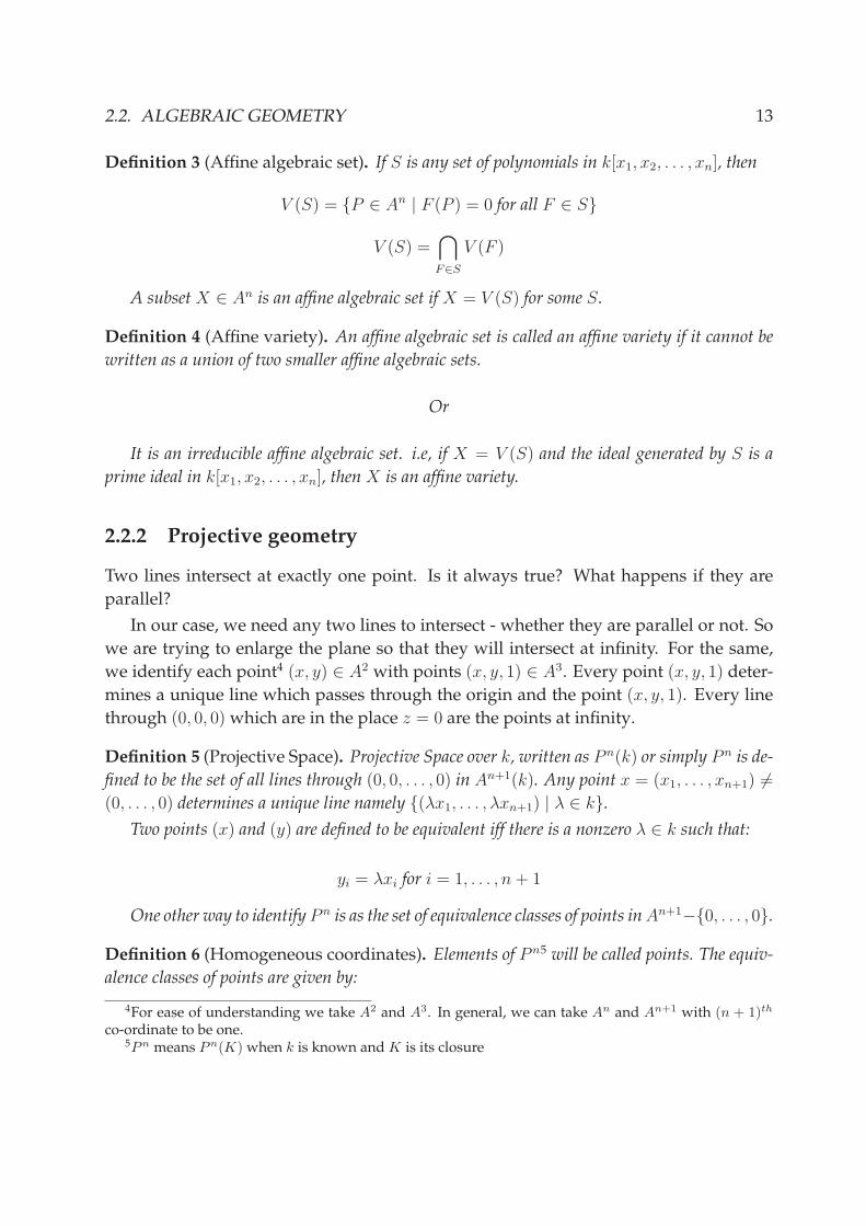
Definition 3 (Affine algebraic set). If S is any set of polynomials in k[x1, x2, . . . , xn], then
V (S) = {P ∈ An | F (P ) = 0 for all F ∈ S}
V (S) =⋂
F∈S
V (F )
A subset X ∈ An is an affine algebraic set if X = V (S) for some S.
Definition 4 (Affine variety). An affine algebraic set is called an affine variety if it cannot be
written as a union of two smaller affine algebraic sets.
Or
It is an irreducible affine algebraic set. i.e, if X = V (S) and the ideal generated by S is a
prime ideal in k[x1, x2, . . . , xn], then X is an affine variety.
2.2.2 Projective geometry
Two lines intersect at exactly one point. Is it always true? What happens if they are
parallel?
In our case, we need any two lines to intersect - whether they are parallel or not. So
we are trying to enlarge the plane so that they will intersect at infinity. For the same,
we identify each point4 (x, y) ∈ A2 with points (x, y, 1) ∈ A3. Every point (x, y, 1) deter-
mines a unique line which passes through the origin and the point (x, y, 1). Every line
through (0, 0, 0) which are in the place z = 0 are the points at infinity.
Definition 5 (Projective Space). Projective Space over k, written as P n(k) or simply P n is de-
fined to be the set of all lines through (0, 0, . . . , 0) in An+1(k). Any point x = (x1, . . . , xn+1) 6=(0, . . . , 0) determines a unique line namely {(λx1, . . . , λxn+1) | λ ∈ k}.
Two points (x) and (y) are defined to be equivalent iff there is a nonzero λ ∈ k such that:
yi = λxi for i = 1, . . . , n + 1
One other way to identify P n is as the set of equivalence classes of points in An+1−{0, . . . , 0}.
Definition 6 (Homogeneous coordinates). Elements of P n5 will be called points. The equiv-
alence classes of points are given by:
4For ease of understanding we take A2 and A3. In general, we can take An and An+1 with (n + 1)th
co-ordinate to be one.5Pn means Pn(K) when k is known and K is its closure

14 CHAPTER 2. MATHEMATICAL BACKGROUND
(x1, . . . , xn+1) ∼ (λx1, . . . , λxn+1); λ 6= 0, xi ∈ k.
If a point P ∈ P n is determined by some (x1, . . . , xn+1) ∈ An+1, we say that (x1, . . . , xn+1)
is a set of homogeneous coordinates for P . In fact, (x1, . . . , xn+1) stands for an equivalence
Definition 7 (Homogeneous Polynomial). A homogeneous polynomial is a polynomial with
all its terms having the same degree.
Or formally,
F (λx1, . . . , λxn+1) = λdeg(f)F (x1, . . . , xn+1) for all λ ∈ K.
Definition 8 (Projective algebraic set, Projective variety). If S is any set of homogeneous
polynomials in k[x1, x2, . . . , xn+1],
V (S) = {P ∈ P n | F (P ) = 0 for all F ∈ S}
V (S) =⋂
F∈S
V (F )
A subset X ⊆ P n is a projective algebraic set if X = V (S) for some S.
A projective algebraic set is called a projective variety if it cannot be written as a union of
two smaller projective algebraic sets.
Or
It is an irreducible projective algebraic set. i.e, if X = V (S) and the ideal generated by S,
represented by I(V ), is a prime ideal in k[x1, x2, . . . , xn+1], then X is a projective variety.
When V (I) is a projective or affine variety then the generator polynomials of I(V )
are irreducible. Otherwise, the union of the factors of these polynomials form the same
ideal, as the roots of the polynomials are the same. Now, the ideal formed is prime ideal.
Suppose, for example that the ideal is generated by only one irreducible polynomial:
I(V ) = F . Then GH ∈ (F ) ⇒ G ∈ (F ) or H ∈ (F ). In other words: F divides G or H .
2.2.3 Affine and projective spaces - relation
We came up with the projective space, in the beginning of this section, to enable any
two lines to intersect at exactly one point. Now we should see how it happens. From
definition 5, we know that a point (x, y, z) ∈ P 2 is equivalent to (x/z, y/z, 1) ∈ P 2 which

2.2. ALGEBRAIC GEOMETRY 15
is the equivalent of (x, y) ∈ A2. Now, we should try to get the points at infinity by
putting z = 0 in (x, y, z) ∈ P 2. We get a point at infinity of A2. Using homogeneous
coordinates and polynomials we can find the intersection of the lines (x, y, z) in the
projective plane z = 0. The intersection represents the point at infinity of A2 which will
be the point of intersection of the lines under consideration. This sounds really absurd.
But we define that all lines in the plane z = 0 and passing through origin corresponds
to directions in the affine space. So we can define the projective space as follows.
P 2 = A2 ∪ {set of directions in A2}
So, all lines in the same direction will intersect at one of these points.
Now, how do we define it formally? We can define the set of direction in A2 by P 1.
So, P 2 = A2 ∪ P 1. Following represents the mapping between the two spaces.
{[a, b, c] : a, b, c not all zero}∼ ↔ A2 ∪ P 1
[a, b, c] →{
(a, b) ∈ A2 if c 6= 0
[a, b] ∈ P 1 if c = 0(2.1)
[x, y, 1] ← (x, y) ∈ A2 (2.2)
[A,B, 0] ← [A,B] ∈ P 1 (2.3)
Definition 9 (Homogenisation and Dehomogenisation). F ∈ k[x1, . . . , xn+1] is called a
form if it is a homogeneous polynomial and we define F∗ = F (x1, . . . , xn, 1). This is called
de-homogenisation.
If we have a polynomial in n variables, we can replace xi by xi/xn+1. This transformation
gives F ∗ from F . This is called homogenisation.
Definition 10 (Algebraic Curve). An algebraic curve is always an algebraic variety of dimen-
sion equal to one. In two dimensional plane (P 2), a projective variety C is called an algebraic
curve when I(C), the ideal of k[x1, . . . , xn+1] which generates C, is generated by a single poly-
nomial ∈ k[x1, . . . , xn+1] which is irreducible by definition.
We denote V (I), [curve generated by ideal I] by C
C : F (x1, . . . , xn+1) = 0 ∈ k[x1, . . . , xn+1]
and I(C) = 〈F 〉.
From here onwards, C is an algebraic curve. Let it be C : F (x1, . . . , xn).

16 CHAPTER 2. MATHEMATICAL BACKGROUND
Definition 11 (Coordinate ring). Coordinate ring of C over k is the quotient ring given by
k[C] = k[x1, . . . , xn]/I(C)
Similarly, the coordinate ring of C over K is defined as
K[C] = K[x1, . . . , xn]/I(C)
An element of K[C] is called polynomial function on C. They are polynomials modulo C.
Definition 12 (Function field and rational functions). The function field k(C) of C over k
is the field of fractions of k[C]. Similarly, K(C) the function field of C over k is the field of
fractions of K[C].
K(C) =
{G
H| G,H ∈ K[C], deg(G) = deg(H)
}
An element of K[C] is called a rational function.
Definition 13 (Zeros and Poles). Let R ∈ K(C)∗ and P ∈ C. If R(P ) = 0, then R is said to
have a zero at P . If R is not defined at P , then R has a pole at P . (We write R(P ) = ∞)
Definition 14 (Uniformising parameter). Let P ∈ C. For all G ∈ K(C)∗, there exist
T, S ∈ K(C)∗,mP ∈ Z such that,
G = TmP S and T (P ) = 0 and S(P ) 6= 0,∞.
The function T is called a uniformising parameter for P .
Definition 15 (Intersection multiplicity). Let G,S ∈ K(C) and P ∈ C. Let T ∈ K(C) be
the uniformising parameter for P :
G = TmP S and T (P ) = 0 and S(P ) 6= 0,∞. Then mP is the intersection multiplicity of G at
P .
Theorem 16 (Bezout’s Theorem ). Let F and G be projective plane curves with degrees m an
n respectively. Assume F and G have no common components. Then :
∑
P∈F∩G
I(P ) = mn
Where I(P ) is the intersection multiplicity at point P and P ∈ F ∩G are the common points
of F and G. i.e, the points of intersections.
Definition 17 (Order of Polynomial functions). The order of a polynomial function G ∈K[C] at a point P ∈ C is the intersection multiplicity at that point and denoted by ordP (G).

2.2. ALGEBRAIC GEOMETRY 17
Definition 18 (Order of rational functions). The order of a rational function R = G/H ∈K(C) at a point P ∈ C is defined as: ordP (R) = ordP (G) − ordP (H).
2.2.4 Divisors
The ideals generated by the polynomial in function field of C are sub-varieties of C. i.e,
the intersection of roots of I(C) and a rational function. We name them as Divisor.
Definition 19 (Divisor). A divisor D is a formal sum of points P ∈ C:
D =∑
P∈C
mP P
with mP ∈ Z and for all but finitely many mP = 0.
The degree of D is the integer deg(D) =∑
P∈C mP .
The order of D at P is the integer ordP (D) = mP .
Definition 20 (support of a divisor). Let D =∑
P∈C mP P be a divisor. The support of D is
the set:
supp(D) = P in C : mP 6= 0
Definition 21 (Addition of divisors). The divisors form a group under addition. The group
of divisors of C are denoted by Div(C). We can add two divisors as follows.
∑
P∈C
mP P +∑
P∈C
nP P =∑
P∈C
(mP + nP )P
The subgroup of Div(C) with divisors of degree 0 is Div0(C).
Definition 22 (GCD of divisors.). Let D1 =∑
P∈C mP P and D2 =∑
P∈C nP P . Then the
gcd(D1, D2) is defined by
gcd
(∑
P∈C
mP P,∑
P∈C
nP P
)=
∑
P∈C
min(mP , nP )P
Definition 23 (Principal Divisor). Let R = G/H ∈ K(C) and G,H ∈ K[C]. The divisor of
a rational function R is called a principal divisor and defined as:
div(R) =∑
P∈C
ordP (R)P
By applying definition 18 at every points of G and H , we know that div(R) = div(G) −div(H). We can see that div(R) ∈ D0.

18 CHAPTER 2. MATHEMATICAL BACKGROUND
Definition 24 (Principal Divisor Group). The principal divisor group is defined by:
P = {Div(R) | R ∈ K(C)}
We have,
P ⊂ Div0(C) ⊂ Div(C).
Definition 25 (Jacobian). The Jacobian of the curve C is defined by the quotient group:
J = J(C) = Div0(C)/P
Let D1, D2 ∈ Div(C). We have the following equivalence relation on Div(C):
D1 ∼ D2 ⇔ D1 − D2 ∈ P
Or equivalently:
D1 ∼ D2 ⇒ ∃R ∈ K(C) : D1 = D2 + div(R)
2.2.5 Genus of a curve
The genus of a curve is better explained with the help of a well celebrated theorem in
mathematics. For any given curve, the problem which is given below gives the value of
genus of the curve and the theorem stated below gives a definition to the genus.
For any divisor D, the set
L[D] = {f ∈ K(C) | (f) + D ≥ 0} ∪ 0
Where (f) is the principal divisor formed by f . L(D) is the space of all rational functions
with poles no worse than D+ (points having positive order) and zeros of multiplicity at
least as specified by D−.
L(D) is a vector space over K The dimension of L(D) is defined to be ℓ(D). The
problem of finding the dimension of the vector space is the Riemann-Roch problem.
Theorem 26 (Riemann’s Theorem). There is a constant g such that ℓ(D) ≥ deg(D) + 1 − g
for all divisors D. The smallest such g is called the genus of C. g is always a non-negative
integer.
The theorem stands as a definition for genus of a curve.

2.3. HYPERELLIPTIC CURVES 19
2.3 Hyperelliptic curves
With the preparation made till here in this chapter, we are ready to see the definition and
properties of Hyperelliptic curves. Hyperelliptic curves are a class of algebraic curves.
They can be seen as generalisations of elliptic curves. We classify them depending on
the genus of the curve. For all genus, g ≥ 1 we have hyperelliptic curves. A detailed,
simple and beautiful tutorial on Hyperelliptic Curves is available in [MWZ96, Kob94].
Definition 27 (Hyperelliptic Curves). Let k be a field and K be the algebraic closure of k. A
hyperelliptic curve C of genus g over k is defined by an equation of the form.
C : y2 + h(x)y = f(x) in k[x, y] (2.4)
Where h(x) ∈ k[x] is a polynomial of degree at most g and f(x) is a monic polynomial of
degree 2g +1 and there are no solutions (x, y) ∈ K2 which simultaneously satisfy y2 +h(x)y =
f(x) and the partial derivatives 2y + h(x) = 0 and h′(x)y − f ′(x) = 0. A singular point on C
is a solution (x, y) ∈ K2 which simultaneously satisfies all these conditions.
So, in other words, a hyperelliptic curve does not have any singular points.
Definition 28 (Rational points, Points at infinity, finite points). Let L be an extension field
of k. The set of L− rational points on C are denoted C(L) and is the set of points P = (x, y) ∈L × L which satisfy the equation 2.4 of curve C together with a special point at infinity 6
denoted by ∞. The set of points C(K) is simply denoted by C. The points in C other than ∞are finite points.
Definition 29 (Opposite, special and ordinary points). Let P = (x, y) be a finite point on
C. The opposite point of P is the point P = (x,−y − h(x)) (Note that P is indeed on C.). We
also define the opposite of ∞ by ∞ = ∞ itself. If a finite point P satisfies P = P , then it is
called a special point. Otherwise P is an ordinary point.
2.3.1 Examples
1. The figure shows a hyperelliptic curve over R.
y2 = (x − 2)(x − 1)x(x + 1)(x + 2)
In this example the genus of the curve is 2. The curve can be seen as the first curve
in Figure 2.1.
6point at infinity is in the projective plane P 2(L).It is the only projective point lying on the line at ∞that satisfies the homogenised hyperelliptic curves equation. If g ≥ two then ∞ is a singular point butallowed since ∞ /∈ L × L

20 CHAPTER 2. MATHEMATICAL BACKGROUND
1 2 3 4 5 6 7 8 9 10−1−2−3−4−5−6
1
2
3
4
5
6
7
−1
−2
−3
−4
−5
−6
−7
Figure 1: y2 = (x − 2)(x − 1)x(x + 1)(x + 2)
1 2 3 4 5 6 7 8 9 10−1−2−3−4−5−6
1
2
3
4
5
6
7
−1
−2
−3
−4
−5
−6
−7
Figure 2: y2 = (x − 1)x(x + 1)

2.3. HYPERELLIPTIC CURVES 21
2. The following figure shows a hyperelliptic curve of genus 1. In other words, this
is an elliptic curve. The curve can be seen as the second curve in Figure 2.1.
y2 = (x − 1)x(x + 1)
3. The hyperelliptic curve given by the equation:
y2 + xy = x5 + 2x4 + x3 − 5x2 + 10
(a) When the curve is defined over the finite field Z11, the valid points are:
(1, 4), (1, 6), (4, 2), (4, 5), (5, 7), (5, 10), (8, 0)∗, (8, 3), (9, 5), (9, 8)
The point which is starred is a special point.
(b) When the curve is defined over the finite field Z7, the valid points are:
(1, 1), (1, 5), (2, 6), (3, 5), (3, 6), (4, 4), (4, 6), (5, 3), (5, 6), (6, 4)
Here we can see that there are no special points.
Definition 30 (Coordinate ring and polynomial functions.). The definitions are same as the
earlier ones.
Coordinate ring of C over k.
k[C] = k[x, y]/(y2 + h(x)y − f(x))
Coordinate ring of C over K.
K[C] = K[x, y]/(y2 + h(x)y − f(x))
Elements of K[C] are called polynomial functions.
Definition 31 (Function field and rational functions). The function field k(C) of C over k
is the field of fractions of k[C]. Similarly, K(C) the function field of C over k is the field of
fractions of K[C].
K(C) =
{G
H| G,H ∈ K[C], deg(G) = deg(H)
}7
An element of K[C] is called a rational function.
7the condition for degree is necessary iff G,H are from the homogeneous coordinate ring [Ful69]

22 CHAPTER 2. MATHEMATICAL BACKGROUND
2.3.2 Divisors
In the last section we saw all the definitions and primary details of divisors of an alge-
braic curve. Those are applicable for a divisor of hyperelliptic curves also.
An example would make it clearer with the case in hand.
Example 32. Let P = (x1, y1) be a point on C. Then,
div(x − x1) =
{P + P − 2∞ P is ordinary ,
2P − 2∞ P is special .
(x − x1) is the line which is parallel to y axis and passes through the point (x1, 0).
The y value of C for the value x1 is y1. The line passes through this point of the curve
C. If the point P is an ordinary point, then there are two y values for the same x. These
points correspond to P and P .
Or
If P is a special point, its opposite also is the same point P and the line passes
through it. So is the divisor.
2.3.3 Semi-reduced divisors
A semi-reduced divisor is a divisor of the form:
D =∑
i
miPi −(
∑
i
mi
)∞
Where each mi ≥ 0 and all the Pi’s are finite points such that if P ∈ supp(D), then
P /∈ supp(D) unless P is special in which case mi = 1.
Fact 33. For each divisor D ∈ D0 there exists a semi-reduced divisor D1(D1 ∈ D0) such that
D ∼ D1.
2.3.4 Reduced divisors
Definition 34 (Reduced Divisor). Let D =∑
i miPi − (∑
i mi)∞ be a semi-reduced divisor.
We call D to be a reduced divisor, if it satisfies the following property.
∑mi ≤ g
Fact 35. For every divisor D ∈ D0, there exists a unique reduced divisor D1 such that D ∼ D1.

2.3. HYPERELLIPTIC CURVES 23
2.3.5 Representations of divisors
Divisors are combinations of points on the curves. There are at least three different ways
of representing divisors. For the purposes of this thesis, only two of them are needed.
Point or explicit representation
This is the simplest form of representation. This is the representation which directly
follows from the definition of the divisor word by word. Here, we represent the divisors
just as the formal sum of points along with the order of points. If P = (xi, yi) are the
points in the support of the divisor and mi’s are the order of point Pi’s respectively:
D =∑
i
miPi
For computational purposes this representation is not advisable. One drawback of
this form is that the values of xi’s and yi’s are in K which is the closure of the field k on
which we have defined our curve.
Mumford representation
This is the representation which is mostly used for the computing. The reasons for the
ease of use in computing will be clear, once the representation is described.
A semi-reduced divisor can be represented with two polynomials. Let D be the
divisor.
D =∑
i
miPi − (∑
mi)∞
The two polynomials are:
1. U(x) = Π(x − xi)mi : This is a monic polynomial of degree
∑mi.
In fact, this is a polynomial which has roots, which have the same x-coordinate as
the points in the support of the divisor. The multiplicities of the roots also is the
same as the order of the corresponding point.
2. V (x) - for the representation of y coordinates. There are two cases here.
(a) If all the points Pis are distinct.
V (x) =∑
i
yi
(Πj 6=i (x − xi)
Πj 6=i (xi − xj)
)

24 CHAPTER 2. MATHEMATICAL BACKGROUND
V (x) is the unique polynomial of maximum degree one less than degree of U .
i.e, deg(V ) ≤ deg(U) − 1. Also, that V (xi) = yi for all xi.
(b) If all the points are not distinct.
We have to find out a V which satisfies the following condition along with
the condition V (xi) = yi.
V (x) =
The unique polynomial of degree smaller than∑i mi − 1 such that if multiplicity of Pi = mi(
ddx
)j[V (x)2 + V (x)h(x) − f(x)]x=xi
= 0
for 0 ≤ j ≤ mi − 1
In other words, V (x) is the unique polynomial such that:
(x − xi)mi | (V (x)2 + V (x)h(x) − f(x))
This, what is seen above is given by the following theorem [MWZ96, Mum84].
Theorem 36. Let D =∑
i miPi − (∑
mi)∞ be a semi-reduced divisor. Where P = (xi, yi) are
the points and mi are the order of the points respectively.
Let a(x) = Π(x − xi)mi and b(x) be a unique polynomial which satisfies:
1. deg(b(x)) ≤ deg(a(x))
2. b(xi) = yi for all i for which mi 6= 0
3. a(x) divides (b(x)2 + b(x)h(x) − f(x))
Then D = gcd(div(a(x)), div(b(x) − y)).
For proof of the theorem [MWZ96] and for more details of Mumford representation
refer [Mum84].
Now we can see whether these polynomials a(x) and b(x) are constructable. a(x) is
easy. For b(x):
1. P = (xi, yi) is ordinary.
Let b(x) =∑
i ci(x − xi)mi be the polynomial we need. It is easy to see that b(x)
satisfies the conditions. We have to find out the constants ci’s. From bi(xi) = yi
we get c0. Then (bi(x)2 + bi(x)h(x) − f(x)) = 0 for x = xi and for all the mi − 1
derivatives. This gives us enough equations to find out the constants.

2.4. JACOBIAN OF A CURVE 25
2. P = (xi, yi) is special. (mi = 1) Here we can directly see that bi(xi) = yi satisfies all
the conditions.
Now, using Chinese Remainder Theorem [Knu97] for polynomials, we can find a
unique polynomial b(xi) ∈ k[x] which can represent the divisor along with a(x).
b(x) ≡ bi(x)(mod(x − xi)mi) for all i
The polynomials a(x) and b(x) together will represent the divisor.
The main advantage of this representation is that we can have the representation in
k[x]. We need not bother about the closure of k. All the calculations also can be done in
k[x]. This we will see later.
2.4 Jacobian of a curve
In the last section we saw the definition of jacobian of a curve. In this section the details
of Jacobian is further explored.
Let D0 = {set of all divisors of degree 0}. The set of divisors of rational functions
form the principal divisors, f{P} ⊂ D0. And the jacobian, J is the quotient group
D0/P .
Let D1, D2 ∈ D0; D1 ∼ D2 if D1 −D2 ∈ P . That is, D1 = D2 + (f) for some f ∈ K(C).
By definition itself J is a group.
2.4.1 Group operation in Jacobian
Jacobian is a group by its definition itself and the operation of divisor addition satisfies
all the group axioms. But for the sake of a formal-ness, one could say that it is the
addition of two reduced divisors.
J is a group of equivalence classes (see facts 33 and 35). Every divisor ∈ J has an
equivalent reduced divisor. In every class of J , there will be a unique reduced divi-
sor. Hence, addition in the jacobian is the addition of two equivalence-classes in the
Jacobian. The classes can be represented by the unique reduced divisor present in each
class8. So, essentially, the addition of two classes boils down to adding two reduced
divisors.
Once two reduced divisors are added, the result is either a reduced divisor or a semi-
reduced divisor. If it is a reduced divisor it already represents the resulting equivalence-
class in which it is a member. On the other hand, if it is a semi-reduced divisor, the
8this is similar to representing Zp by the smallest positive numbers which can represent the class

26 CHAPTER 2. MATHEMATICAL BACKGROUND
reduced divisor equivalent to the semi-reduced divisor to represent the resulting class
(there are algorithms to compute the representative reduced divisor of an equivalence
class).
Let [D1] and [D2] be the two classes to be added. And the result be [D3].
[D1] + [D2] = [D3]
This is done by:
D1r ⊕ D2r = D3r
Where D1r represents [D1], D2r represents [D2] and D3r represents [D3] and all Dir are
reduced divisors. And ⊕ stands for the addition of the divisors and then the reduction.
How do we do this in practice? For the addition in the jacobian, we have many
algorithms available. They use different types of representations of the divisors, which
are explained in one of the following sections (Section 2.6). Before looking into the
details of the algorithms, let us have a look to the different representations of divisors.
Definition 37 (k-rational Divisor). Let P (x, y) be a point on C and σ be an automorphism of
K over k. Then P σ = (xσ, yσ) also is a point on C.
A divisor D =∑
mP P is a k-rational divisor if Dσ =∑
mP P is equal to D for all auto-
morphisms σ of K over k.
A divisor is k-rational does not mean that all the points are k-rational.
2.5 Frobenius endomorphism
Let g be a positive integer and let Fq be a finite field of q = pn elements. Let C be the
hyperelliptic curve defined by y2 = f(x) where f(x) is a monic polynomial of degree
2g + 1 with coefficients in Fq and with distinct roots. The roots (coordinates) may be in
the base-field or in an extension field. Let J represent the Jacobian of the curve.
Let us now consider a q-power Frobenius endomorphism φ(x) = xq. The elements of
Fq are not affected by φ, but in the extension fields, it is non-trivial. The map transforms
the points on the curve by transforming their coordinates. For the same reason, the
mapping extends to divisors, by changing the points.
But on closer look, the action of changing a divisor is also the changes on the coef-
ficients of the Mumford representation of the divisor. Since the divisor is defined over
Fq, the mapping φ may permute its points but the divisor is left without any change.

2.5. FROBENIUS ENDOMORPHISM 27
2.5.1 Characteristic polynomial
The Frobenius operator φ acts linearly and it has a characteristic polynomial of degree 2g
with integer coefficients. In genus two, the characteristic polynomial has the following
form.
χ(X) = X4 − s1X3 + s2X
2 − s1qX + q2
so that χ(φ) is the identity map on all of J .
According to “Riemann hypothesis for curves”, on the roots of the zeta functions of
curves, which was proved by Weil, the complex roots of χ have absolute value√
q. In
genus 2, the bounds for it are | s1 |≤ 4√
q and | s2 |≤ 6q.
2.5.2 Bounds on cardinality - Weil Interval
The Frobenius is very closely related to the number of points on the curve and also to
the divisors in J , over the base field and its extensions.
Theorem 38. Let J be the Jacobian variety of a hyperelliptic curve C. The group of Fq rational
points on J is denoted by J(Fq). Let χ(t) be the characteristic polynomial of the qth-power
Frobenius endomorphism of C, then the order of the Jacobian is given by #J(Fq) = χ(1).
From the theorem it is clear that the knowledge of χ is equivalent of counting the
jacobian.
There are two additional results in the case of genus two curves. If #C(Fqi) is the
number of points of C in Fqi , the following are true.
#C(Fq) = q − s1
#C(Fq2) = q2 − s12 + 2 · s2
These details help in fixing an interval for the order of the Jacobian. The small interval
is called the Hasse-Weil interval.
⌈(√q − 1)2g⌉ ≤ #J(Fq) ≤ ⌊(√q + 1)2g⌋
It is also clear, if the order of jacobian is known, determining the characteristic polyno-
mial becomes easier.

28 CHAPTER 2. MATHEMATICAL BACKGROUND
For genus 2
The width of the Hasse-Weil interval is close to 4gqg− 12 . In case of genus 2, w = 2⌊4(q +
1)√
q⌋.
2.6 Addition algorithms for divisors
In section 2.4.1, we saw how the Jacobian of a hyperelliptic curve acts as a group and
how the group law functions. In this section we will see the various methods for group
addition.
2.6.1 Geometrically what is it?
We are concerned about the addition of reduced divisors of a genus g hyperelliptic
curve. Consider that we have two reduced divisors, D1 and D2.
D1 =∑
i
miPi −(
∑
i
mi
)∞ and D2 =
∑
i
miQi −(
∑
i
mi
)∞
where the Pi and Qi are points on C.
The idea is to find out a curve which passes through the points Pi and Qi with corre-
sponding intersection multiplicities so that the intersection cycle of the curve will give
D1 + D2. Let us draw that curve. We can see that this new curve will intersect with a
few more points of C. Now we have to draw a new curve which passes through the
opposites of the new intersections with the same multiplicities of their opposites9. This
new intersection cycle is the resulting reduced divisor which is the desired sum D1 +D2
For ease of explanation, we will consider curve of genus 2. So we have:
D1 = P1 + P2 − 2∞ and D2 = Q1 + Q2 − 2∞
From geometry, we know that these points determine a unique cubic polynomial
b(x) which passes through them with respective multiplicities (in this case all multiplic-
ities are 1). Substituting b(x) for y in the equation of the hyperelliptic curve, we get:
b(x)2 + b(x)h(x) = f(x) (2.5)
Solving the equation gives us 6 solutions (points on the curve) of which 4 of them are
9The reason for this is to have an identity element [ST92, Sil86]

2.6. ADDITION ALGORITHMS FOR DIVISORS 29
known to us. Let the new points be R1 and R2. Then the new divisor D3 = R1 + R2−2∞is the sum of D1 and D2.
2.6.2 Examples
Example 39. A more visual representation of the aforementioned group law can be seen
in the first picture in Figure 2.2.
Blue and red lines are divisors D1 and D2 respectively. The new polynomial b(x)
is represented by the green curve. It intersects the hyperelliptic curve at six points in-
cluding P1 and P2 of D1, Q1 and Q2 of D2 and the new points R1 and R2. Then we can
calculate the opposites of these new points and get R1 and R2 respectively. The new
curve (magenta) is the resultant divisor.
Example 40. We will see a more concrete example. Let us take a hyperelliptic curve of
g = 1 which is an elliptic curve. How is the addition done in that case. As the genus is
one, the reduced divisor is nothing but a single point P and also the multiplicity cannot
exceed one. So our D1 and D2 are nothing but two points P and Q.
y2 = (x − 2)x(x + 4)
We have the elliptic curve with points P and Q to be added together. We find out a
line(curve) passing through them. This new line passes through the point R. Now we
take the reflection of R on x-axis. The reflection R is the sum of P and Q.
The group law is depicted in the second picture in Figure2.2.
2.6.3 Algebraic methods
In the last section we got a feel of how to add divisors. In the case of elliptic curves
it was very easy. But in the general case, drawing a curve is not an easy thing. What
we can do is that algebraically find out the equation of the curves/divisors. This is not
very difficult. In fact, we can use the representations we saw in the last section. The one
which is most popular is Mumford representation. The polynomials a(x) and b(x) have
all information about the divisors. Also there is a method which uses Chow forms.
Cantor’s Algorithm
In 1987 Cantor [Can87] came up with an algorithm for the addition of reduced divisors
of hyperelliptic curves. The algorithm is known as Cantor’s algorithm. As we have two

30 CHAPTER 2. MATHEMATICAL BACKGROUND
1 2 3 4 5 6 7 8 9 10−1−2−3−4−5−6
1
2
3
4
5
6
7
−1
−2
−3
−4
−5
−6
−7
b
b
b
b
b
b
b
b
b
b
b
b
P1
P2 Q1
Q2
R1
R2
R1
R2
Figure 1: Addition of divisors in hyperelliptic curves
1 2 3 4 5 6 7 8 9 10−1−2−3−4−5−6
123456789
101112
−1−2−3−4−5−6−7−8−9
−10−11−12
P
Q
R
R
Figure 2: Group law in group of points of elliptic curves

2.6. ADDITION ALGORITHMS FOR DIVISORS 31
phases for addition of divisors, the algorithm also has two phases. Cantor’s method
uses Mumford representation.
1. Composition : This is the phase in which we find out the new divisor which is the
sum of the input divisors.
2. Reduction : In this phase we prune out the parts which are not needed and take
the inverse of the resulting one to get the result.
Composition
• Input: Reduced divisors D1 = div(a1, b1) and D2 = div(a2, b2) both defined over k.
• Output: A semi-reduced divisor D = div(a, b) defined over k such that D ∼ D1 +
D2.
1. Use the extended Euclidean algorithm to find polynomials d1, e1, e2 ∈ k[u] where
d1 = gcd(a1, a2) and d1 = e1a1 + e2a2
2. Use the extended Euclidean algorithm to find polynomials d, c1, c2 ∈ K[u] where
d = gcd(d1; b1 + b2 + h) and d = c1d1 + c2(b1 + b2 + h)
3. Let s1 = c1e1, s2 = c1e2 and s3 = c2, so that
d = s1a1 + s2a2 + s3(b1 + b2 + h) (2.6)
4. Set
a = a1a2 = d2 (2.7)
b =s1a1b2 + s2a2b1 + s3(b1b2 + f)
dmod a (2.8)
Again, I am not providing the proof. In fact, the proof given by Cantor contained a
few errors and later when Koblitz gave the algorithm, he did not give any proof. But
for the proof, readers can refer [Kob98, Can87, MWZ96].

32 CHAPTER 2. MATHEMATICAL BACKGROUND
Reduction
Reduction part is comparatively simpler and easy to understand. Here also we skip the
proof - for details [Kob98, Can87, MWZ96]. But here, the algorithm is pretty clear that
no one needs a proof to see that it is indeed correct.
Input: A semi-reduced divisor D = div(a, b) defined over k.
Output: The (unique) reduced divisor D′ = div(a′, b′) such that D′ ∼ D.
1. Set
a′ = (f − bh − b2)/a (2.9)
b′ = (−h − b) mod a′ (2.10)
2. If degx(a′) ≥ g then set a ← a′, b ← b′ and go to step 1.
3. Let c be the leading coefficient of a′, and set a′ ← c−1a′
4. Output(a′, b′).
Other versions
As we told in the introduction, we are looking for faster addition in the jacobian of
hyperelliptic curve. The method given above is a polynomial time algorithm. But when
it comes to the number of micro-instructions needed in a processor, this version of the
algorithm is too general to implement. So we have many different refined version of this
algorithm or slight variants of this algorithm which is tailor made for different genus
hyperelliptic curves.
Harley’s Algorithm
In the year 2000, Rob Harley [Har00] came up with an algorithm which is very similar to
the original Cantor’s algorithm. The algorithm was optimised and made for genus two
curves [GH00]. In the tailor made method for genus two curves, addition and doubling
are handled separately. Finally the number of operations comes up to two inversions,
three squarings and 24 multiplications for the genus 2 case.

2.7. ECDLP AND HECDLP 33
Explicit formulae by Tanja Lange
In her paper in 2002, Tanja Lange [Lan02] gives explicit formulae for arithmetic on genus
two curves over fields of even characteristic and for arbitrary curves. The formula is
faster than all the methods which existed before that. It allows to obtain fast arithmetic
on hyperelliptic curves of genus 2. The algorithm is a case by case analysis of different
situations which can arise.
2.7 ECDLP and HECDLP
In the earlier section 2.1.2, we saw that, in the multiplicative group Z∗p, the discrete
logarithm problem is: given elements r and q of the group, and a prime p, find a number
k such that r = qkmod p.
In the previous sections we also introduced new types of groups: the groups of
points on the Jacobian of hyperelliptic curves. It is also to be noted that elliptic curves
are hyperelliptic curves of genus 1. They also have a jacobian and the jacobian is simply
the group of points on an elliptic curve. The main advantage of these groups - the
points on an elliptic curve or the jacobians of hyperelliptic curves - compared to the
multiplicative groups of finite fields, is that under certain conditions, there is no method
like index calculus known to solve the DLP. If the groups are chosen with care, then the
most efficient way to solve the DLP is by means of Pollard’s rho method [Pol78].
For this method, one has to perform roughly√
#J group operations. This means
that its running time is exponential in lg #J , and one can use smaller groups for achiev-
ing the same level of security.
2.7.1 Elliptic Curve Discrete Logarithm Problem
The points on an elliptic curve form a group under addition. The elliptic curve dis-
crete logarithm problem could be defined as: given points P and Q in the group, find a
number that k · P = Q; k is called the discrete logarithm of Q to the base P .

34 CHAPTER 2. MATHEMATICAL BACKGROUND
Example:
In the elliptic curve group defined by
y2 = x3 + 9x + 17 over F23
What is the discrete logarithm k of Q = (4, 5) to the base P = (16, 5)?
In comparison with the example given in section 2.1.2, one can already see that
this question is very hard.
The (naive) way to find k is to compute multiples of P until Q is found. The
first few multiples of P are:
P = (16, 5); 2P = (20, 20); 3P = (14, 14); 4P = (19, 20); 5P = (13, 10); 6P =
(7, 3); 7P = (8, 7); 8P = (12, 17); 9P = (4, 5)
Since 9P = (4, 5) = Q, the discrete logarithm of Q to the base P is k = 9.
In a real application, k would be large enough such that it would be infeasible to
determine k in this manner.
2.7.2 Hyperelliptic Curve DLP
As the name itself indicates, HECDLP is the general version of ECDLP. Unlike having
the points on the curve, which is used in ECDLP, HECDLP depends on the group of
reduced divisors for defining the DLP.
The hyper elliptic curve discrete logarithm problem could be defined as: given di-
visors D1 and D2 in the group, find a number that k · D1 = D2; k is called the discrete
logarithm of D2 to the base D1.
As mentioned earlier, the main advantage of HECDLP is the lack of existence of
any sub-exponential algorithms to solve it. With today’s computers it is reasonable to
assume that it is unfeasible to perform 280 operations in a reasonable amount of time.
Under this assumption, it follows that cryptosystems based on elliptic or hyperelliptic
curves are secure if #J ∼ 2160. As a consequence, these systems are more efficient, and
allow shorter key sizes than their multiplicative group counterparts. The details of the
sizes needed were explained in Table 1.1.

Chapter 3
The State Of The Art
“Do not worry about your difficulties in Mathematics,
I can assure you, mine are still greater.
- Albert Einstein.
In the previous chapter, we saw how the points (or divisors) of a hyperelliptic can
form a group, which is called the jacobian of the curve. We also did see that the count
(cardinality) of this group is vital in deciding the level of security the curve can offer.
In this chapter, the methods which already exist for calculating the order of groups are
sketched.
We will start by examining the algorithms which can be used for generic groups
and then observe how these algorithms are tailor suited for the special cases of jaco-
bian. Counting methods which leverage the properties of hyperelliptic curves also are
explained.
A note on notation: All through this chapter, G is the group of which the order is to
be computed; M is the upper-limit of the order and α is a random element which has
the order N .
3.1 Existing methods for counting
Owing to the property of groups that the order of the group is a multiple of the order of
the elements of the group (or even the same sometimes), the very naive method starts
by finding the order of an element α.
The order of an element is the number for which the exponent of the elements pro-
duces the unit element of the group. So, one starts by finding the exponents of α until
the unit element of the group is produced.
35

36 CHAPTER 3. THE STATE OF THE ART
α, α2, α3, . . . αN
Since the order o of the group is the number for which the the N th power of every
element in the group is same as the unit element, quite often the order of an element is
the same as that of a group.
If they are not the same, one could find out the orders of different elements of the
group and find out the least common multiple of them which is either the order of the
group or a large factor of it.
Determining the order of a group (or α) using the above outlined method is very
expensive. The larger the order of α, the more expensive the computation becomes. The
complexity of the algorithm is O(N).
There are two methods which are based on the aforementioned idea, but better in
complexity. The goal of the algorithm is to find an n such that αn = 1G where 1G is the
unit element. So it suffices to find two powers of α which are equal.
If i and j are two numbers for which αi = αj , then we know, αj−i = 1G and that j − i
is the number being sought. It is possible that j − i is not n, but a multiple of n.
3.1.1 Baby Step Giant Step - BSGS
One of the methods which leverages the idea of finding a multiple of α is the baby step
giant step method. It was proposed by Shanks [Sha71] and it finds the order of the
element.
All what is needed is an upper limit of the group order.
Assuming the order of the group is M , the algorithm takes a random α from the
group and computes two sets of its exponents. As the name of the method indicates,
one set is created using baby steps and the other using giant steps.
Baby Steps
Every exponent of α is calculated and stored in a list up to√
M . Along with the values,
the exponent-value of α is also stored.
This set can otherwise be seen as the set of αk for k <=√
M .
Giant Steps
Exponents of α is computed for every multiples of√
M until M . This set is αj for j =
i ×√
M

3.1. EXISTING METHODS FOR COUNTING 37
After computing each exponent, it is checked whether the value is present in the first
list created by baby steps. If it is present there, then the result is at hand.
If one of the giant steps is present in the baby steps, the number j and k mentioned
in the previous section is found out.
The algorithm can proceed to compute the N (or a multiple of it) by finding the
difference of the exponents which produced the same value.
Example:
Consider a group, G which has an order close to one million. Using the initial naive
method, one has to compute every exponent of α for all values 1, 2, . . . , 1000000.
In baby-step-giant-step method, one can compute the powers of α as below.
α, α2, α3, . . . α1000
Then, compute and check each of the following until a match is found. The smallest
difference in the powers which give the same exponent would be N .
α1000, α2000, α3000, . . . α1000000
The complexity of the algorithm is O(√
N) to calculate N .
3.1.2 Birthday paradox method
This method, which is also known as Pollard’s Rho method, is based on the well known
birthday paradox. The idea of birthday paradox is that if we randomly take√
k elements
from a set of size k, there is a good chance we will pick an element twice1. For more
details, please see [Pol78].
While putting the birthday paradox into use for order computation, we guess a ran-
dom sequence of powers of α and we are bound to have a repetition sooner or later.
The algorithm starts by randomly guessing powers of α, check whether that value
was computed earlier. If it was, the j and k of the previous section are available and
their difference is the order of α. If the power was not computed earlier, it is added to
the list and the algorithm continues.
Just as in the baby-step-giant-step method, the complexity of the algorithm is O(√
N).
1If there are at least 23 people in a room, the chance that two of them share the same birthday is high

38 CHAPTER 3. THE STATE OF THE ART
3.1.3 Order counting with Primorial
In [Sut07], A. Sutherland proposed a method of making the counting of the order of a
group easier, by using some rudimentary facts about groups. In effect, computing the
order relies on Pollard’s methods. But the rudimentary methods help to save resources.
The order of an element of a group is always a factor of the order of the group. If a
rough idea about the upper limit of group order is available, one can carefully choose
an element for which the order has no factors smaller than prime P .
The idea is to start with a random element α, and with M being the upper limit of
the group order. According to the Primorial method, one finds the largest power of 2,
smaller than M - let’s call it k and computes β = α2k
. From the properties of the group,
β has an order which is co-prime to 2.
One can do the same with all prime numbers - 2, 3, 5, . . ..
β = αΠpkp
By computing a β with order coprime to the small primes, in the traditional group
order algorithms, the numbers which are coprime to the product of all the primes can
be avoided and a great saving in time/space is achieved.
3.2 Counting in the Jacobian
If we consider a hyperelliptic curve over R, or even over the complex numbers, it is
meaningless to talk about counting the number of points, because it is infinite.
But once we define a curve over a finite field, the number of points is not infinite
anymore and becomes important because of the application of the curves and the sig-
nificance played by the number of points (order of jacobian).
One could imagine any kind of finite field over which a hyperelliptic curve can be
defined. Let us broadly put them into two classes - fields of characteristic 2 and fields
with an odd prime as the characteristic.
3.2.1 Fields with small characteristic
Many results are available for counting points over finite fields of characteristics p,
mainly with the use of p-adic liftings. The complexity of these methods is exponen-
tial in ln p. Hence for small primes (especially for p = 2) these methods are good. Using
these algorithms, it is possible to compute orders of Jacobian varieties in sizes of cryp-
tographic usage over fields with small characteristic.

3.2. COUNTING IN THE JACOBIAN 39
The main result with small fields is available at [Ked01, GG01].
3.2.2 Fields with larger/arbitrary characteristic
The story takes a not-so-happy turn when the counting has to be done over fields of
arbitrary characteristic. There are a few results of which only one is considered to be of
practical use: Gaudry-Harley [GH00, Gau05].
3.2.3 Gaudry-Harley method
The Gaudry-Harley algorithm consists of two main parts. In the first part, details about
the order of the Jacobian is computed based on different results.
The detail which is computed is the residue modulo m,m ∈ Z>0 of the order of
the given jacobian variety. The details of extracting this information is described in the
following section.
Once the residue modulo m is calculated, in the second phase of the algorithm, a
parallelised Pollard’s lambda method is used in finding the number which matches
the acquired information and also the properties of the group order. This square root
algorithm was taking the lion’s share of computing resources in the Gaudry-Harley
algorithm.
The initial part of the algorithm, where the residue modulo m details are computed,
has two smaller sections.
Cartier Manin
For hyperelliptic curves, the characteristic polynomial of the Frobenius modulo p is con-
nected with the Hasse-Witt matrix of the curve. The g × g matrix (Hasse-Witt) can be
computed using the following result.
Theorem 41. Let y2 = f(x) represent a hyperelliptic curve with genus g. Let the coefficient of
xi in the polynomial f(x)(p−1)
2 be represented by ci. Then the Hasse-Witt matrix is given by:
A = (cip−j)1≤i,j≤g
In [Man65, GH00], the above result is connected to the residue modulo p of Frobe-
nius. For a matrix A = (aij), let Ap be the element-wise pth-power. i.e., (apij).
Theorem 42. Let C be a curve of genus g defined over a finite field Fpn . Let A be the Hasse-
Witt matrix of C, and let Aφ = AAp . . . A(pn−1). Let k(t) be the characteristic polynomial of the

40 CHAPTER 3. THE STATE OF THE ART
matrix Aφ, and χ(t) the characteristic polynomial of the Frobenius endomorphism. Then
χ(t) ≡ −1gtgk(t) mod p
Armed with this knowledge, it is straight forward to compute χ(t) modulo the char-
acteristic p and hence #J(Fq) mod p. One must notice that this method would be feasible
only for not too large p. In practice, any p > 1000000 is too expensive.
This is a very efficient way of knowing about the Jacobian order, for moderately large
p.
Schoof’s Improvement
A detailed explanation of Schoof’s method (extended by Gaudry) is beyond the scope
of this thesis. A more interested reader is recommended to read [Kam91, Pil90].
In a nutshell, the hyperelliptic analogue of Schoof’s algorithm2 is about computing
χ modulo l for small primes. Once this has been done for sufficiently many primes,
Chinese remainder theorem [Knu97] is used to compute χ. From the bounds which
were mentioned above, the primes are bounded by l = O(lg q).
For the methods of computing χ mod l, the reader is encouraged to peruse [Kam91,
Can94].
Modified Pollard’s Lambda
From the Cartier Manin operator and Schoof’s method, different details of o(J) is com-
puted as o(J) ≡ n1 mod p, o(J) ≡ ni mod lki , for l = 2, 3, 5, . . ., k ∈ Z.
Using Chinese remainder theorem the aforementioned information is combined to
o(J) ≡ n mod m where m is the product of p and all values of lk.
The birthday paradox algorithm which was mentioned earlier in the chapter can be
modified to avoid computing the values which are not in the form of n mod m. Using
the modified algorithm, computing resources can be saved up to an order of√
m.
For further details, see [GH00]
3.3 Can this be improved?
So far in the thesis, we discussed about the counting in the Jacobian of hyperelliptic
curves of genus 2. In this section, we give a more clear description of our goal.
2Originally designed for elliptic curves
3.3. CAN THIS BE IMPROVED? 41
In section 3.2.3, we saw the state of the art methods for generic curves. It was also
seen that the running time of the algorithm is too long to have any practical use in cryp-
tosystems. We also have seen a few of the generic methods of group order counting.
The goal of this thesis is to bring the best out of the both the worlds. i.e., to try to ap-
ply the advances of generic group order counting in the special setting of hyperelliptic
curves, where one has the advantage of
• Weil Interval
• Cartier Manin operator
• (modified) Schoof’s method
The details of how they can be applied together are explained in the next chapter.
The next chapter also shows what an improvement is achievable.

42 CHAPTER 3. THE STATE OF THE ART
Chapter 4
The Solution
“The art of doing mathematics consists in finding that special case
which contains all the germs of generality.”
- David Hilbert
In this chapter, we develop a faster method for counting in the jacobian of hyper-
elliptic curves (of genus 2). Starting with the naive solution which tries to apply the
Primorial method [Sut07] in the jacobian, the chapter witnesses the gradual develop-
ment of an algorithm which combines all the special knowledge available (about the
jacobian).
The final algorithm has an improvement factor of ϕ(P )P
1 over the conventional method.
Even though the computational complexity of the algorithm is the same as the tradi-
tional one, the improvement is a quite good, in computing in the jacobian of practically
useful hyperelliptic curves2.
A note on notation: In this chapter, P is the Primorial (multiple of primes up to p),
and T is the totient of P , m is the characteristic of the field on which the curve is defined.
The variables w, l and u represent the Weil interval, its lower and upper boundaries -
respectively. #J stands for the size of the jacobian.
1where P is the product of the first p primes. The value of p depends on the size of the jacobian2In this chapter, a hyperelliptic curve (of genus two) which is practically applicable is assumed to be
on a field of size 280 which in turn means, the size of the jacobian is ∼ 2160 and size of Weil interval is∼ 2120.
43

44 CHAPTER 4. THE SOLUTION
Size(crv) Size (Jac) P Reduction Pϕ(P )
Speed-Up√
PPϕ(PP )
Work % Days (7 × %)
10 20 11 4.812 2.193 45.584 3.19020 40 17 5.539 2.353 42.488 2.97430 60 29 6.331 2.516 39.742 2.78140 80 31 6.542 2.557 39.096 2.73650 100 41 6.892 2.625 38.091 2.66660 120 47 7.209 2.685 37.242 2.60770 140 59 7.474 2.734 36.576 2.56080 160 67 7.714 2.777 36.003 2.52090 180 71 7.824 2.797 35.748 2.502
Table 4.1: Improvements for different curves.
4.1 Primorial Vs Weil
Counting in the jacobian (of hyperelliptic curves) is easier than the counting in any other
group of similar size, primarily owing to the knowledge of the search intervals.
But the traditional algorithms and the Primorial method, which we have in hand, are
not fine tuned for searching in intervals. So, the naive attempt could be the application
of the Primorial method to see whether the improvements promised by it would be
good enough to surpass the benefit of Weil’s interval.
A hyperelliptic curve defined over a field of size q has a jacobian of the size compa-
rable to N = q2. Using the traditional methods of counting implies that the search has a
complexity√
N = q. See [GH00].
Using the Primorial method, one can avoid a large share of the search space. Ta-
ble 4.1 gives an idea of how much improvement in search can be achieved for different
sizes of groups. The sizes (represented in bit-size) are of the field over which the curve
is defined and the jacobian respectively.
The last column is the number of days needed for the algorithm to finish running,
assuming that the non-Primorial version would need a week (7 days) to finish.
The size of the Weil interval is of the order of q1.5 for genus 23. So, Weil interval is a
very small fraction (q−12 ∼ 2−40for a practically useful curve) of the whole jacobian of a
hyperelliptic curve, where as the Primorial savings is of the order of less than 65%.
Naive Primorial reduces the search space to two thirds, where as the whole Weil-
interval itself is one in 240th of the Jacobian. Therefore, the naive method of trying to
apply the Primorial method directly on the whole jacobian of a curve is extremely more
expensive than using the Weil knowledge.
3The weil interval is specified as ⌈(√q − 1)2g⌉ ≤ #J(Fq) ≤ ⌊(√q + 1)2g⌋. For more details see 2.5.2

4.2. PRIMORIAL AND WEIL 45
4.2 Primorial and Weil
Since the naive method of applying the Primorial directly on the Jacobian is not very
promising, the advantage of Weil’s interval has to be taken into consideration.
Note: Primorial method only guarantees that the order of the chosen (created)
element is co-prime to the selected primes (Please see 3.1.3). The order of the
group is a multiple of this order and need not be co-prime to the primes chosen.
Instead of the naive method of searching in all over the jacobian, the search has to
be modified to specific intervals inside the jacobian.
1. The Weil interval [l, u] is initially searched for the element order. There search
would be successful only if the group order is the same as the order of the element,
or the group order is a product of the order of the element and a number which is
co-prime to the Primorial4.
2. Since the order of the Jacobian is sure to be within the Weil interval and since
the order of the divisor has to be a factor of it, if the order was not found in the
case above, we can avoid the searches is such ranges where the order cannot be
present and move on to the intervals where the probability of finding the order is
non-zero.
For example, the range [wu
2, wl] is sure not to have the order - because no multiple
of any number in that interval is within the Weil interval.
So, if the order was not found in Weil interval, the search has to continue tow2, w
3, . . . = [l, u], [ l
2, u
2], . . .. until the order of the element is found.
Considering the search spaces as described above, the counting algorithm has to
look in a set of special intervals (defined by Weil interval). Which in other words mean
that set of intervals could be skipped while doing BSGS. The following set contains all
such intervals.
{[l
i,
u
i + 1
]| 1 ≤ i < r =
u
w
}
The remaining search space - from 1 to wu minus the above set, will provide us with
the size of the real search space.
4While using the primorial method, the orders computed are coprime to the primorial. Order of theelement is assured to be coprime to the primorial. If the order of the group is a multiple of the order of theelement, the multiplier has to be coprime to the primorial, otherwise it would never have been computed.

46 CHAPTER 4. THE SOLUTION
S =u
1− l
1+
u
2− l
2+ . . . +
u
r− l
r+
u
r + 1
=w
1+
w
2+ . . . +
w
r+
u
r + 1= S1 + S2
> w
[1 +
lg r
2
]+ S2
= w
[1 +
lg q12
2− 3
]+ S2
4.2.1 Put in perspective
From the above equation, if we calculate the search space S, that will be S = 19w + S2.
As mentioned in the previous section, even for large primes (the ones used for Primorial
at cryptographic sizes, usually less than 67), the factor c = ϕ(p)PP
is about than 0.25
Using the Primorial advantage along with the reduced search space, the resulting
search space would be f · S = 4.95 · w + 0.25 · S2. This value is definitely larger than w,
the Weil interval.
From this, it is clear that there is no advantage of using the Primorial method, if we
know a small interval where we expect the order to be present.
Using Primorial method along with Weil interval is actually more expensive than
the method without Primorial. This arises from the fact that a non-Primorial method
has to do the search only inside the Weil interval, where as Primorial method needs a
search outside the interval.
4.3 Including Cartier Manin operator
Using the Cartier-Manin operator (see 3.2.3 and [Man65]), some more details of the
group order can be obtained, provided the characteristic of the underlying field is not a
very large prime number5.
The group order can be represented in terms of m, the characteristic of the field as
follows:
#J = Nr mod m
5Any prime larger than 106 is considered too large.

4.3. INCLUDING CARTIER MANIN OPERATOR 47
As the original Primorial method avoids making the (computing the) unnecessary
babysteps or giantsteps based on the knowledge of co-primeness of the order to initial
primes, a new method could incorporate this special knowledge above for avoiding the
computation of baby/giant-steps which are not of the form as in the equation above.
The method to find out the jacobian using baby-step-giant-step method is sketched
as Algorithm 1.
Algorithm 1: Compute Jacobian order: Cartier Manin and Primorial BSGS
Data: J , w, wl, wu, m, Nr, α - random element of JResult: #J - Order of the jacobianbegin
Nr ←− CartierManinOn(J,m);p, P ←− BestPrimorial(w,Nr);T ←− BestLimitBabies(w,Nr, P );β ←− DivisorWithSpecialOrder(α, p);
* Generating the babysteps *;B0 ←− {k · m − Nr | 0 < k ≤ (1 + T/m)};B1 ←− {j ⊥ pp | j ≤ T, j ∈ Z
+};B ←− B0 ∩ B1;Babysteps ←− ∅;for x ∈ B do
Babysteps ←− Babysteps ∪ {x · β};end
* Generating giants and checking against babysteps *;Giants ←− {g | wl ≤ g ≤ wu; m,T divides g};for x ∈ Giants do
if x · β ∈ Babysteps then#J ←− ComputeDifference(x,Babysteps) ;
end
endreturn #J
end
Details of Functions
In the algorithm 1, there are some functions which are not yet been well defined. A
description of each of them is given below. The functions being standard and straight-
foreward, the pseudo-code for the same are avoided.
CartierManinOn(J,m): As described in section 3.2.3, the CartierManin operator can

48 CHAPTER 4. THE SOLUTION
be used to find the remainder of #J when divided by m, the characteristic of the
field. Please see [Man65] for further details.
BestPrimorial(w,Nr): Once the values of Weil interval and the special knowledge of
#J are obtained, the best prime number for the algorithm can be decided. This
function is explained below.
BestLimitBabies(w,Nr, P ): The number of babysteps and giantsteps are defined by up-
per limit of the babystep. This function finds out the optimal value of the limit,
based on the available inputs.
DivisorWithSpecialOrder(α, p): The element which is to be used for baby-steps and
giant-steps has to meet the requirement that its order should be co-prime to the
Primorial (i.e., co-prime to each of the prime numbers ≤ p). To compute such a
divisor, β, a random divisor is chosen and it is exponentiated to all the powers of
the prime numbers in question. For more details, see section 3.1.3 or [Sut07].
4.3.1 The Cost - Reduction and Estimation
Like the traditional BSGS, the cost is based on the number or babysteps and giantsteps
to be made before the order can be computed. The best result is achieved when these
two numbers are roughly the same. See [Coh96].
The cost can be found out by looking at the two functions which are mentioned
above.
BestPrimorial(w,Nr): It would seem that the larger the size of the Primorial, the lesser
the number of computations needed. But the increase in the size of the Primorial
is advantageous to the computation only up to a limit. And this limit depends on
the size of the search space. In the normal scenario, where the restriction of Nr is
unknown, the optimal value of Primorial is the one closest to√
w · Pϕ(P )
, which is
also used as the upper bound of baby steps. See [Sut07].
But with the introduction of Nr, the number of babysteps in the same interval is
reduced by a factor of Nr, where as the number of giantsteps remain the same.
To share the advantage of Nr between the babysteps and giantsteps equally, the
optimum value of the Primorial moves higher by a factor of√
Nr.
Hence, the optimal value of Primorial would be the Primorial closest to√
w · Pϕ(P )
· Nr
BestLimitBabies(w,Nr, P ): Once the best Primorial has been established, computing
the upper-bound is all what is needed for starting babysteps. Looking at the gi-
antsteps, one can see that the giantsteps has to be divisible by m because of the

4.4. INCLUDING SCHOOF’S IMPROVEMENT 49
properties of babysteps. Each giantstep has to be also divisible by the upper-
bound. Hence, the upper-bound shall be a multiple of m. Now with this knowl-
edge, the upper-bound can be fixed as the multiple of m closest to the optimal
Primorial which was computed in the previous step.
Improvement from traditional methods
In terms of complexity of the methods, the use of CartierManin or Primorial has not
reduced the complexity from O(N12 ). But by the reduction in the number of steps,
the employment of both Cartier Manin and Primorial methods provides a reduction
of√
m · Pϕ(P )
in the computations.
Proof
Using the Cartier Manin operator reduces the size of search space by a factor of m, the
characteristic of the field over which the curve is defined. As the complexity of the
algorithm is O(√
n), an speed up of√
m is attained.
While using Primorial, only those numbers which are co-prime to P are used for the
baby-steps or for giant-steps.
The number of numbers co-prime in every P numbers is ϕ(P ). In the Weil interval,
there fore the total number of giant-steps + baby-steps is reduced by another factor of√ϕ(P )
P.
Therefore, both the methods of CM and Primorial gives a speed increase of√
m · Pϕ(P )
4.4 Including Schoof’s improvement
In this section and the following section, we will see the final products of this thesis. In
this section, we work on improving the counting method by incorporating the details
obtained by Schoof’s method in knowing some more information about the Jacobian
order.
For further details on Schoof’s method, please see [Sch95, Can94].
Schoof’s method provides information about the jacobian in a similar fashion like
Cartier Manin.
#J = ns mod 2k · l

50 CHAPTER 4. THE SOLUTION
Where l is the product of initial primes up to p1. Usually, in practice, the value
of p1 is less than 17, for the reason that computation of modulo p becomes expensive
exponentially. Details of the computation could be seen at [GH00].
So, the details of the order of the jacobian available are as below.
#J = Nr mod m
#J = ns mod 2k · l#J ⊥ P
Using Chinese Remainder Theorem [Knu97], the first two of the modulos can be
combined as follows.
#J = n mod m · 2k · l#J = NmodM
Even with the additional Schoof’s method, one can re-formulate the counting prob-
lem in a way similar to how it was when only Cartier Manin operator was used, which
is helpful in using the same (or slightly modified) method, provided the new problems
are ironed out.
4.4.1 The trouble introduced
Before the introduction of modulo by Schoof, the modulo and the Primorial were co-
prime6. In fact, the common factor of m, Nr and P was 1, before the introduction of
Schoof’s method.
But if the common factor d is not 1, then no single integer in the Weil interval which
satisfies the modulo would be coprime to the Primorial, P . In the last section, where
CartierManin operator was used, there is a subset of integers which satisfy the modulo
which are not coprime to P .
6m is a large prime number and P is the product on initial primes

4.4. INCLUDING SCHOOF’S IMPROVEMENT 51
4.4.2 The algorithm
In a nutshell, the solution tries to generate babies and giants which satisfy the conditions
and produce the results. But the names shall not confuse the reader, and make her think
that babysteps always have to be first. In our solution, we are generating the giants
steps initially and the babysteps are made to match the giantsteps stored.
An optimal value for the size of the giant step is computed using the available values
of Primorial and the m. Using this value, the giantsteps are made in the Weil-interval
and are saved. As the next step, the babysteps are produced. Unlike in the earlier cases,
where we suggested searching in the small intervals if the searched value was not found
in the original one, here we suggest to adjust the value of the Primorial to accommodate
the generation of more babysteps - which is the equivalent of going to lower-intervals7.
The method mentioned above is sketched in Algorithm 2.
Details of Sections of the algorithm
As mentioned above, the algorithm has 3 sections which are explained here one by one.
Choosing the optimal giantstep size
Similar to what we saw in the previous algorithm, the introduction of Cartier
Manin results and the Primorial values reduces the search space by a large fac-
tor. Schoof’s method throws new light to the Jacobian order, thereby reducing the
search space further8.
The reduction of the space by a factor k directly implies that the size of the gi-
antstep would be√
k times larger than the traditionally optimal size.
But, the size of the giantstep has to be a multiple of P and also m (m in #J =
n mod m), for the babysteps are going to be of the form P⊥b = l ·m − n, for l ∈ Z.
Considering these two restrictions, one has to choose, g, the size of a giantstep
as close as it can be to√
w · k, where w is the size of Weil-Interval; where g is a
multiple of m and P .
As shown in the code, we choose the Primorial chosen for a case without Schoof’s
and CM information available, and remove the larger primes until the size of the
giantstep is in the neighborhood of the optimum size.
7The reader would note that, since the giantsteps are made initially and stored, it would be a waste ofresources to make another set of giantsteps for every “miss” in the search interval
8Reduction in space does not imply that the size of the interval has become less, but that many of theintegers in the interval can be excluded from the potential candidates for group order

52 CHAPTER 4. THE SOLUTION
Algorithm 2: Compute Jacobian order: Cartier Manin, Schoof and Primorial BSGS
Data: J , w, wl, wu, m, Nr, p, P , α - random element of JResult: #J - Order of the jacobianbegin
Nr ←− CartierManinOn(J,m);p, P ←− BestPrimorial(w,Nr);T ←− BestLimitBabies(w,Nr, P );β ←− DivisorWithSpecialOrder(α, p);
* Find the optimal Giant Size *;while True do
lpm ←− lcm(pr,m);g ←− Multiple of lpm after
√w;
opt ←−√
w·pr·m
ϕpr;
if g too larger than opt thenRemove the larger primes one by one;
elseBe satisfied with it, BREAK;break;
end
end
* Generating giants steps *;Giants ←− {gi = g · i | wl ≤ gi ≤ wu; i ∈ Z};
* Generating the babysteps *;Primes = {All primes inpr};foreach i < g do
if i⊥pr and i = nmodm thenResult ←− CheckBabyStep(i, Giants);if Result then
return Resultend
end
endforeach pi in Primes do
prx ←− pr
pi;
foreach i < g doif i not checked yet & i⊥prx & i = nmodm then
Result ←− CheckBabyStep(i, Giants);if Result then
return Resultend
end
end
endend

4.4. INCLUDING SCHOOF’S IMPROVEMENT 53
Loop Hole: The while loop could be infinite.
The algorithm has a while loop which seemingly runs into an infinite loop. But
here is the proof that it will terminate, where the worst case is P being reduced
to 1.
As the primes are removed one by one, the size of the suggested value would
get closer to the optimal value and finally up to the next multiple of m larger
than the optimal value which has to be set as the safe-neighborhood for satis-
fying the condition to break out of the loop.
Generation of Giantsteps.
This section of the algorithm is the easiest but the more space consuming one.
Once the size of the giantstep has been fixed up on, the algorithm can compute
the giantsteps between the Weil-Interval.
It is worth noting that unlike the traditional babystep-giantstep algorithm, giants
are generated and stored for further searches. This of course comes with the dis-
advantages of having multiplications with larger multipliers.
All the giantsteps are multiples of P and also m.
Generation of Babysteps.
The babystep generation is worth noting because of the different sweeps through
the giantstep space for completely generating them, instead of doing them in a
single sweep.
In the initial sweep, the steps which are coprime to the Primorial are chosen to be
generated and compared against the giantsteps in the store. This is the equivalent
of searching for the the order of α, the random element inside the Weil-interval.
To be precise, the babysteps which are of the form l · m − n, which are coprime
to the Primorial P are computed. Since the giants are all multiples of P and m, if
the order happens to be in Weil-interval, there will be a match between one of the
babysteps and one of the giantsteps.
It is worth observing that, a match in the first sweep means the order of the
group is the same as the order of α, the element in question.
Once all the potential candidates, which are coprime-multiples of α, are generated
and checked against the giantsteps, and if it leads to no match, the implication is
that the order of the element is a factor of the group order.

54 CHAPTER 4. THE SOLUTION
Then the algorithm proceeds to explore the intervals where the order of the ele-
ment is in the intervals w2, w
3, . . .
This is achieved by taking off the primes from the Primorial one by one and gen-
erating the babysteps which are coprime to the new Primorial, and which are not
generated in the earlier sweeps.
This process continues until the Primorial becomes one - which is falling back to
the normal babystep-giantstep algorithm.
4.5 Proof
The proof of the algorithm explained above needs two sections: (i) It terminates and
(ii) It finds the right solution.
4.5.1 The algorithm terminates
The algorithm has three loops of which one is seemingly an infinite loop. In the above
section, we saw that the loop which seems an infinite loop does terminate in all cases.
The second loop in the algorithm is for the generation of the giantsteps. It exe-
cutes exactly wg
, where w is the size of the Weil-interval and g is the size of the optimal
giantstep-size determined.
The third section of the algorithm makes l sweeps through the whole interval [1, g]
where g is the size of the optimal giantstep-size, which guarantees that the algorithm
terminates. (Where l is the number of primes in the Primorial)
4.5.2 It gives the deemed result
To prove that the algorithm gives the deemed result, two points are to be noted.
• Irrespective of the value of the optimal giantstep-size, the algorithm creates wg
gi-
antsteps in the Weil-interval.
• Through the l sweeps through the interval [1, g], the algorithm generates all the
babysteps which satisfy α × (k · m − n).
Considering that all the babysteps up to g are checked against all the giantsteps
which are separated by g in the Weil-interval, a match is sure to occur between one of
the babysteps and one of the giantsteps.
The details of the proof is the same as in section 3.1.1.

4.6. COST ANALYSIS 55
4.6 Cost analysis
The cost of the algorithm is the number of group operations required for computing the
size of the group order. The number of operations required is the sum of the number of
giantsteps and of babysteps made during the computation.
Let the size of the giantstep be:
g = c ·√
w · P · mϕ(P )
Where c is the constant which decides the optimum value.
This implies that the number of giantsteps be:
#g =w
g=
1
c·√
w · ϕ(P )
P · m
For the number of babysteps, we could consider the best and worst cases.
Best Case
In the best case, the order of the element is a non-trivial factor of the group order, which
means the first sweep of babysteps would get a match from the giantsteps.
Which means, the number of operations = g·ϕ(P )P
.
Therefore, the number of operations would be of the order of O(√
w·ϕ(P )P ·m
).
Worst Case
In the worst case, the order of the element is a very small factor of the group order,
which means that the number of sweeps of babysteps is l, the number of primes in the
Primorial.
This implies that the number of operations = g which is of the order of O(c ·√
w·P ·mϕ(P )
).
The constant c could be leveraged to adjust the value of g.
A value c = ϕ(P )P
makes sure that the worst case is always better than the Schoof-
CartierManin method without the use of Primorials.

56 CHAPTER 4. THE SOLUTION
4.6.1 In practice
In the case of jacobians and their elements, an average case could not make sense. But
from the above discussion confirms that the algorithm2 has a better running time than
the Schoof-CartierManin algorithm. Please see [GH00].
Where as the best case saves up to 60% of the work (For details of percentage savings,
please refer to table 4.1).
In the next section, the above algorithm will be applied in the cryptographic setting
where one could make sure that the best case of the algorithm would only be put to use.
4.6.2 In theory
The improvement which algorithm promises is in terms of the order P , but not in terms
of the size of the field on which the hyperelliptic curve is defined. Even though the size
of the Primorial depends on the size of q, it is very weakly related and is not strongly
coupled to make a polynomial difference in the cost.
At the same time, the introduction of the Primorial method provides with an im-
provement factor of√
Pϕ(P )
, which ranges from 2 to 3. To know what percentage of
change it would make, please see table 4.1.
4.7 Cryptographic restrictions
All through the previous sections in this chapter, we examined the different cases of
using the available information about the jacobian order, in finding out the order of any
arbitrary hyperelliptic curve.
In the last section (Section 4.4), it was even shown that the combination of the avail-
able information can be leveraged to design an algorithm (Algorithm 2) which substan-
tially reduces the cost.
In this section, we will look at the requirements of a cryptosystem, for guaranteeing
security on the forms of protocols/methods it offers. In section 2.7, we saw that the
jacobian offers no sub-exponential algorithms for the solution of DLP defined on it. This
statement is true only for those curves which are of genus less than 3. Please see [SV].
Even though there aren’t any sub-exponential algorithms, there are some attacks
which have been developed for breaking the cryptosystems based on hyperelliptic curves.
Here in the rest of the section, we shall see the effective ones among them, which are re-
lated to the order of the group and we shall see what kind of countermeasure is applied
to get around these problems.

4.7. CRYPTOGRAPHIC RESTRICTIONS 57
Pohlig-Hellman
If the group order #G of G factors as Πriei then it is possible to reduce the DLP in
G to a DLP in subgroups of order ri, see [PH78]. So if r is the largest prime divisor
of #G, then the DLP in G is as hard as the DLP in the subgroup of order r. For
this reason it is important to choose G such that its order is almost prime, i.e. such
that #G
ris small. A typical choice is to require that this quotient is ≤ 4. Ideally,
one would like #G to be prime, but it is not always possible to achieve that. For
example, an elliptic curve, or hyperelliptic curve of genus 2 over a field F2l , that is
not super-singular always yields a group of even order.
MOV and Frey-Rück Attacks
Let r be the largest prime divisor of the group order #G. Let k be the smallest
positive integer such that r | qk − 1. Then there is a computable injective group
homomorphism from the order-r subgroup of G to F ∗qk , see [9] and [31]. If k is too
small, then one can solve the DLP in G by first mapping it to F ∗qk , and use index
calculus there. So one should avoid groups for which k is small. Typically, k > 20
is a safe choice. A random curve is very unlikely to yield a group for which k is
small. There is however a special class of curves, super-singular curves, for which
k is always small.
Anomalous curves
If the largest prime divisor r of #G is equal to the characteristic of Fq, then one
can transform the DLP to a DLP in the additive group of Fq, where it is trivial to
solve. See [42] and [38]. So this should be avoided.
Weil restriction and cover attacks
Let C be an elliptic curve or hyperelliptic curve of genus g defined over an exten-
sion field Fqe . Let G be the group C(Fq) if C is elliptic, or JC(Fq) if C is hyperellip-
tic. Then sometimes it is possible to find a curve X defined over Fq such that there
is a homomorphism from G to JX(Fq) that transfers the DLP from G to JX(Fq). If
the genus of such an X is not much bigger than e · g, then index calculus methods
on X enable one to compute the DLP faster than with Pollard’s rho method. The
original idea behind this construction goes back to Frey, and it has been applied
successfully to attack several curves, for the first time in [10].
4.7.1 Good curves
To summarise which curves are safe to use, here is the list of the required properties. Let
q be either a prime, or q = 2l, with l prime. Let C be an elliptic curve or a hyperelliptic
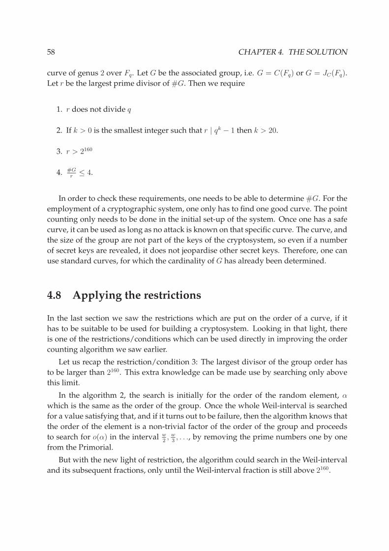
58 CHAPTER 4. THE SOLUTION
curve of genus 2 over Fq. Let G be the associated group, i.e. G = C(Fq) or G = JC(Fq).
Let r be the largest prime divisor of #G. Then we require
1. r does not divide q
2. If k > 0 is the smallest integer such that r | qk − 1 then k > 20.
3. r > 2160
4. #G
r≤ 4.
In order to check these requirements, one needs to be able to determine #G. For the
employment of a cryptographic system, one only has to find one good curve. The point
counting only needs to be done in the initial set-up of the system. Once one has a safe
curve, it can be used as long as no attack is known on that specific curve. The curve, and
the size of the group are not part of the keys of the cryptosystem, so even if a number
of secret keys are revealed, it does not jeopardise other secret keys. Therefore, one can
use standard curves, for which the cardinality of G has already been determined.
4.8 Applying the restrictions
In the last section we saw the restrictions which are put on the order of a curve, if it
has to be suitable to be used for building a cryptosystem. Looking in that light, there
is one of the restrictions/conditions which can be used directly in improving the order
counting algorithm we saw earlier.
Let us recap the restriction/condition 3: The largest divisor of the group order has
to be larger than 2160. This extra knowledge can be made use by searching only above
this limit.
In the algorithm 2, the search is initially for the order of the random element, α
which is the same as the order of the group. Once the whole Weil-interval is searched
for a value satisfying that, and if it turns out to be failure, then the algorithm knows that
the order of the element is a non-trivial factor of the order of the group and proceeds
to search for o(α) in the interval w2, w
3, . . ., by removing the prime numbers one by one
from the Primorial.
But with the new light of restriction, the algorithm could search in the Weil-interval
and its subsequent fractions, only until the Weil-interval fraction is still above 2160.

4.8. APPLYING THE RESTRICTIONS 59
4.8.1 Some facts
A hyperelliptic curve which could be used for cryptographic purposes satisfies the fol-
lowing.
• The field Fq over which the curve is defined is of the order ∼ 280
• The order of the jacobian would be closer to ∼ 2160
• The largest prime divisor of #J has to be larger than ∼ 2160
• Using the Primorial method requires the Primorial to contain primes up to 67 < 26
(please see 4.1)
If the choice of Fq is wisely made, the algorithm from the previous section could be
modified to leverage the facts mentioned above, to decide whether a hyperelliptic curve
is safe for cryptography or not, and if safe, to compute the order of the jacobian.
The tailor-made jacobian counting algorithm can be seen in Algorithm 3.
Details of Sections of the algorithm
The algorithm 3 is the same as the algorithm 2 except for the generation of babysteps.
As in the previous method, the babysteps which are all of the form k · m − n for k a
positive integer and the steps being coprime to the Primorial are generated first.
In the next step, where each prime number is taken away from the Primorial, so as
to check for the order of the element in lower intervals, the algorithm checks whether
the upper limit of the interval is smaller than the restriction set by security measures.
And if it is, the algorithm can specify that the curve is not suited for cryptography
and quits.
4.8.2 Analysis and Advantages
Instead of making l sweeps through the giantstep size, the new algorithm makes only k
sweeps until the kth prime divides the Weil-interval to get an interval which has upper
limit smaller than 2160.
By wisely choosing the field over which the curve is defined, and also choosing the
optimal giantstep size as O(c ·√
w·P ·mϕ(P )
), the number of giantsteps would be:
#g =w
g=
1
c·√
w · ϕ(P )
P · m

60 CHAPTER 4. THE SOLUTION
Algorithm 3: Compute Jacobian order: Cartier Manin, Schoof and Primorial BSGS- Tailor made for hyperelliptic curves for cryptographic purposes
Data: J , w, wl, wu, m, P , Nr, α - random element of JResult: #J - Order of the jacobianbegin
Nr ←− CartierManinOn(J,m);p, P ←− BestPrimorial(w,Nr);T ←− BestLimitBabies(w,Nr, P );β ←− DivisorWithSpecialOrder(α, p);
* Find the optimal Giant Size: See 2*;
* Generating giants steps: see 2*;
* Generating the babysteps *;Primes = {All primes inpr};foreach i < g do
if i⊥pr and i = nmodm thenResult ←− CheckBabyStep(i, Giants);if Result then
return Resultend
end
endforeach pi in Primes do
if wu
pilt2160 then
The curve is not suited for cryptography;Exit the algorithm and choose another Curve;
endprx ←− pr
pi;
foreach i < g doif i not checked yet & i⊥prx & i = nmodm then
Result ←− CheckBabyStep(i, Giants);if Result then
return Resultend
end
end
endend

4.9. SUMMARY 61
and the number of babysteps would be:
#b = k · g · ϕ(P )
P · m = c1 ·√
w · ϕ(P )
P · mAnd the cost of the algorithm in terms of the operations needed is #b + #g =
O(√
w·ϕ(P )P ·m
).
4.9 Summary
From the beginning of the chapter, where we started with the naive method of counting
in the jacobian of a hyperelliptic curve, we have developed a solution which reduces
the work to a fraction of the search needed by the naive solution.
In our pursuit to better solutions, we did see some solutions which pointed that the
Primorial method cannot be better than the Weil-interval when there are no other extra
information available.
But, the combination of all the information, has made it possible to devise a method
which is better than the solutions which we saw in the chapter 3 “State of the Art”,
where the best solutions which exist till date are mentioned.
Also, by taking into consideration, the restrictions on a group for guaranteeing se-
curity, we designed a tailor-made method for hyperelliptic curves of genus two, for
deciding whether the curve is good for computation or not. That solution has a silver
lining that, the solution gives the jacobian order, only if the curve fits the required pre-
requisites and a large portion of the unnecessary computation is avoided if the curve is
not good enough.
After seeing the theoretical improvement of√
Pϕ(P )
, the details of implementation
and results are given in the next chapter.

62 CHAPTER 4. THE SOLUTION

Chapter 5
Implementation, Results and Future
Prospects
“This principle is so perfectly general that,
no particular application of it is possilbe”
- George Polya.
The algorithms which were discussed in the chapter 4 were implemented and were
run against the previously-existing algorithms.
In this chapter, we will see the details of the implementation and the results obtained.
We also would look into the future of the research in the direction we are following.
5.1 Implementation
Even though the chapter 4 talks only about the search algorithms, the implementation
of the jacobian counting system required more than just the search algorithms. The
complete implementation was divided into two phases and were run in two different
locations owing to some technical restrictions.
5.1.1 Generating the Curve
The initial phase of the curve consisted of generating enough random curves on random
fields. This phase also consisted of computing the Cartier Manin and Schoof numbers
of the curve.
63

64 CHAPTER 5. IMPLEMENTATION, RESULTS AND FUTURE PROSPECTS
Since MAGMA [MAG] has many of the routines needed for the aforementioned op-
erations, this part of the implementation was done with Magma on a Sun Sparc machine
with shared 16GB memory.
Even though the first phase has no direct connection with the solutions we discussed
earlier, this was an integral part of the project.
Details of implementation (including MAGMA code and BASH scripts) are available
at [Sad].
5.1.2 Counting Algorithms
For the implementation of the counting algorithms, we used SAGE [Ste07] and PythonTM .
Sage provides many useful methods for hyperelliptic curve implementation. The incli-
nation towards open source software acted as an additional reason behind the imple-
mentation of second phase in the open-source mathematical software.
The details of implementation, including the scripts and SAGE code, are available at
[Sad].
5.2 Results: Old Vs. New - Comparison Tables
As a part of testing the implementation, we generated a collection of hyperelliptic curves
(randomly). Potential (random) prime numbers in a valid range1 was chosen and de-
pending on the size (bit size) of the prime numbers, a suitable extension was selected
and the curves were built with random coefficients.
The details of these curves are given in the Curve Database: B.1, B.2, B.3, B.4, B.5.
In this section, we provide the reader with the details and results of running of the
best algorithm from chapter 4 and the algorithms which were designed in the previous
chapter.
The results are widely categorised into two parts -
(i) Based on the advantage of the new methods over the old method.
(ii) Based on the size of the prime numbers and extensions.
If the reader wishes to have more information about the curve, she is kindly
requested to look up the serial number (Column #) of the curve in the Curve
Database: B.1, B.2, B.3, B.4, B.5.
1The characteristic of the base field has to be less that 106 for viable computation of the Cartier Maninoperator

5.2. RESULTS: OLD VS. NEW - COMPARISON TABLES 65
5.2.1 Most of the curves
The table 5.1 compares the running times of the CMSchoof algorithm and the algo-
rithm 2 explained in the previous chapter.
The columns of the table are:
• The serial number of the curve
• The characteristic of the field
• The time required for the CMSchoof algorithm in section 3.2.3
• The time taken by the Primorial method 2
• The order of the curve computed by the two methods
The reader could see that the total time (last row) taken by the Primorial method is
only about 60% of the time required by the CMSchoof method from section 3.2.3.
In table 5.2, the same computation of the group order is given with the break down
of number of babysteps and giantsteps which were computed for the CMSchoof and
Primorial methods respectively2.
As in the previous tables, the last row show the total of the computations needed
for all the curves in the table. The total computation required by the Primorial-Schoof
combination 2 is only 75% of the methods without the Primorial advantage.
5.2.2 The curves which faired well
With some curves, the new method was so fast that we considered it worth mentioning
here. The tables 5.3, 5.4 show the time and operation comparisons between the two
different methods which are the main theme of this chapter.
5.2.3 Curves on non-prime fields
In the initial parts of this section, we saw the comparison of algorithms when they were
applied on curves which were defined on prime-fields.
In the tables 5.5, 5.6, 5.7, 5.8, the reader could see the comparison of algorithms when
the curves are of fields of prime power.
2It is to be observed that the giantsteps and babysteps are interchanged for the Primorial-Schoof com-bination

66 CHAPTER 5. IMPLEMENTATION, RESULTS AND FUTURE PROSPECTS
Characteristic CM-Schoof Primorial Group Order# (in seconds) (in seconds)4 950611 1.92 0.69 9053104956797 914701 1.77 0.74 83613944050211 949733 1.27 0.81 90016565255212 915251 1.77 0.74 83779341694416 931597 1.86 0.70 86998236156220 943153 0.95 0.90 89014290092836 935971 1.74 0.71 87524367442641 910471 1.32 0.72 82933854590443 941557 1.31 0.69 88614013900848 976471 1.94 1.13 95444598483949 910421 1.32 1.22 82911274810452 950329 1.30 0.64 90239447947254 953773 0.98 0.99 90894498249657 983513 1.30 0.85 96727607567666 907363 1.76 0.78 82313744338667 910177 1.90 1.36 83036423523371 926701 1.30 0.96 85765401454478 994927 1.32 0.88 98893078192880 960931 1.35 1.21 92515816143283 968467 1.30 0.56 93674352579285 969421 1.82 0.71 93971033326288 970859 1.01 0.54 94345097443289 944491 1.31 0.74 89126470989691 961871 1.29 0.86 924578774816101 976991 1.31 0.64 953972995396104 995833 1.88 1.22 992188599049105 930779 1.36 1.07 867626285192106 945289 1.34 0.55 894471514876107 979651 1.89 1.02 960456115583109 980887 1.34 0.60 962324055304113 978683 1.89 0.80 959357530602114 994501 1.86 1.10 988997216327115 968729 1.85 1.00 939179183518116 994751 1.86 1.26 990686610702117 931003 1.31 1.22 867403320348118 916291 1.81 1.09 840590700384120 989557 0.99 0.54 978269804256
55.8 32.3
Table 5.1: Comparison old vs. new methods: Time and Group Order

5.2. RESULTS: OLD VS. NEW - COMPARISON TABLES 67
Schoof Primorial Schoof Primorial Schoof Primorial# Base Ext Baby Giant Giants Baby Total Total4 950611 1 37 1 26 38 63 397 914701 1 36 3 15 37 51 40
11 949733 1 26 8 7 19 33 2712 915251 1 36 3 19 37 55 4016 931597 1 36 2 29 37 65 3920 943153 1 18 11 11 10 29 2136 935971 1 36 2 14 37 50 3941 910471 1 26 6 14 19 40 2543 941557 1 26 5 12 19 38 2448 976471 1 37 11 23 38 60 4949 910421 1 26 17 14 19 40 3652 950329 1 26 4 11 19 37 2354 953773 1 19 13 7 10 26 2357 983513 1 26 9 13 19 39 2866 907363 1 36 4 17 37 53 4167 910177 1 36 17 28 37 64 5471 926701 1 26 11 9 19 35 3078 994927 1 26 9 10 19 36 2880 960931 1 26 17 19 19 45 3683 968467 1 26 2 9 19 35 2185 969421 1 37 2 18 38 55 4088 970859 1 19 3 11 10 30 1389 944491 1 26 6 10 19 36 2591 961871 1 26 9 11 19 37 28
101 976991 1 26 4 11 19 37 23104 995833 1 37 13 21 39 58 52105 930779 1 26 14 17 19 43 33106 945289 1 26 2 16 19 42 21107 979651 1 37 9 22 38 59 47109 980887 1 26 3 14 19 40 22113 978683 1 37 4 25 38 62 42114 994501 1 37 11 18 38 55 49115 968729 1 37 9 22 38 59 47116 994751 1 37 15 24 38 61 53117 931003 1 26 17 15 19 41 36118 916291 1 36 11 23 37 59 48120 989557 1 19 3 7 10 26 13
1102 290 592 965 1694 1255
Table 5.2: Comparison old vs. new methods: Number of operations

68 CHAPTER 5. IMPLEMENTATION, RESULTS AND FUTURE PROSPECTS
Characteristic CM-Schoof Primorial Group Order# (in seconds) (in seconds)101 976991 1.31 0.64 95397299539652 950329 1.30 0.64 90239447947243 941557 1.31 0.69 886140139008120 989557 0.99 0.54 9782698042564 950611 1.92 0.69 905310495679106 945289 1.34 0.55 89447151487641 910471 1.32 0.72 829338545904109 980887 1.34 0.60 96232405530489 944491 1.31 0.74 89126470989683 968467 1.30 0.56 93674352579216 931597 1.86 0.70 86998236156288 970859 1.01 0.54 943450974432113 978683 1.89 0.80 959357530602
Table 5.3: Comparison old vs. new: Time and Group Order (Better Curves)
Schoof Primorial Schoof Primorial Schoof Primorial# Base Ext Baby Giant Giants Baby Total Total
101 976991 1 26 4 11 19 37 2352 950329 1 26 4 11 19 37 2343 941557 1 26 5 12 19 38 24
106 945289 1 26 2 16 19 42 21120 989557 1 19 3 7 10 26 13
4 950611 1 37 1 26 38 63 3941 910471 1 26 6 14 19 40 25
109 980887 1 26 3 14 19 40 2289 944491 1 26 6 10 19 36 2583 968467 1 26 2 9 19 35 2116 931597 1 36 2 29 37 65 3988 970859 1 19 3 11 10 30 13
113 978683 1 37 4 25 38 62 42356 45 195 285 551 330
Table 5.4: Comparison old vs. new: Number of operations(Better Curves)

5.2. RESULTS: OLD VS. NEW - COMPARISON TABLES 69
Characteristic CM-Schoof Primorial Group Order# (in seconds) (in seconds)124 1009 1.03 4.18 1040604009999134 647 0.93 3.84 176319369215140 691 1.00 3.88 229310730495
Table 5.5: Curves : Time and Group Order (Better Curves)
Schoof Pri. Schoof Pri. Pri. Schoof Pri. Pri.R# Base Ext Baby Giant Giants Baby Restr. Total Total Total
134 647 2 1295 1451 1294 1156 165 2589 2607 1616124 1009 2 1427 1764 1427 1156 165 2854 2920 1929140 691 2 978 828 977 1156 165 1955 1984 993
3700 4043 3698 3468 495 7398 7511 4538
Table 5.6: Comparison old vs. new: Number of operations(Better Curves)
In the tables where the operations are compared for curves on non-prime fields,
it is seen that the operations needed by Primorial methods are more than the
naive CMSchoof method without Primorial.
But the tables which compare the non-prime based curves have two extra
columns which specify, how the algorithm 3 comes to help from saving the
extra computation by making use of the known cryptographic restrictions.
It is worth noting that the saving done by the restricted (Pri.R) algorithm is
about 50% of the CMSchoof algorithm which is the best one available.
Characteristic CM-Schoof Primorial Group Order# (in seconds) (in seconds)136 197 1.32 5.90 58536332836258130 109 1.15 5.14 1683002823435123 211 1.21 5.93 88361163800489143 149 1.18 5.50 10966612124981
Table 5.7: Comparison old vs. new: Time and Group Order (Better Curves)
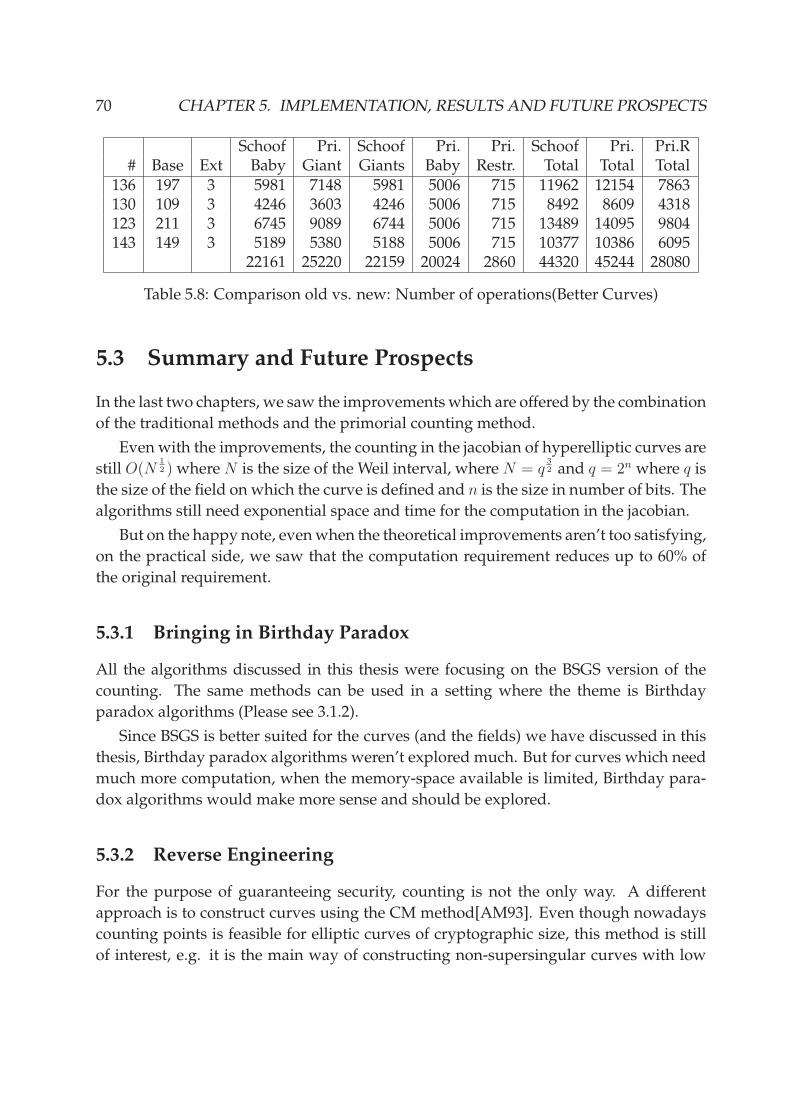
70 CHAPTER 5. IMPLEMENTATION, RESULTS AND FUTURE PROSPECTS
Schoof Pri. Schoof Pri. Pri. Schoof Pri. Pri.R# Base Ext Baby Giant Giants Baby Restr. Total Total Total
136 197 3 5981 7148 5981 5006 715 11962 12154 7863130 109 3 4246 3603 4246 5006 715 8492 8609 4318123 211 3 6745 9089 6744 5006 715 13489 14095 9804143 149 3 5189 5380 5188 5006 715 10377 10386 6095
22161 25220 22159 20024 2860 44320 45244 28080
Table 5.8: Comparison old vs. new: Number of operations(Better Curves)
5.3 Summary and Future Prospects
In the last two chapters, we saw the improvements which are offered by the combination
of the traditional methods and the primorial counting method.
Even with the improvements, the counting in the jacobian of hyperelliptic curves are
still O(N12 ) where N is the size of the Weil interval, where N = q
32 and q = 2n where q is
the size of the field on which the curve is defined and n is the size in number of bits. The
algorithms still need exponential space and time for the computation in the jacobian.
But on the happy note, even when the theoretical improvements aren’t too satisfying,
on the practical side, we saw that the computation requirement reduces up to 60% of
the original requirement.
5.3.1 Bringing in Birthday Paradox
All the algorithms discussed in this thesis were focusing on the BSGS version of the
counting. The same methods can be used in a setting where the theme is Birthday
paradox algorithms (Please see 3.1.2).
Since BSGS is better suited for the curves (and the fields) we have discussed in this
thesis, Birthday paradox algorithms weren’t explored much. But for curves which need
much more computation, when the memory-space available is limited, Birthday para-
dox algorithms would make more sense and should be explored.
5.3.2 Reverse Engineering
For the purpose of guaranteeing security, counting is not the only way. A different
approach is to construct curves using the CM method[AM93]. Even though nowadays
counting points is feasible for elliptic curves of cryptographic size, this method is still
of interest, e.g. it is the main way of constructing non-supersingular curves with low

5.3. SUMMARY AND FUTURE PROSPECTS 71
embedding degree which can be useful in pairing based protocols if one wants to avoid
supersingular curves for some reason or if a larger embedding degree is desired.
While our interests are in creating curves suitable for cryptography, the future re-
search could follow this lead too. The readers who are interested are encouraged to
peruse [Wen03] and [MKS].

72 CHAPTER 5. IMPLEMENTATION, RESULTS AND FUTURE PROSPECTS

Appendix A
Algebra Refresher
This chapter has been provided as an easy reference to the terms used in the thesis.
For detailed references for group theory Herstein [Her86, Her75] and for field theory
Roman [Rom] are recommended. Set theory is assumed to be known.
A.1 Groups
Definition 43 (Group). A nonempty set G is said to be a group if in G there is defined an
operation ⊕ such that it satisfies the following.
1. Closure: a, b ∈ G implies a ⊕ b ∈ G
2. Associativity: Given a, b, c ∈ G then a ⊕ (b ⊕ c) = (a ⊕ b) ⊕ c
3. Existence of Identity: There exists a special element ǫ ∈ G such that a⊕ ǫ = ǫ⊕ a = a for
all a ∈ G. ǫ is called the identity element of G.
4. Inverse Element: For every a ∈ G there exists an element b ∈ G such that a⊕b = b⊕a = ǫ.
(We write b as a−1 and call it the inverse of a in G)
These four conditions are called group axioms.
We usually represent a group by (G, ∗); where G is the group and ∗ is the group
operation.
Example 44. (Z, +) is a group where Z is the integers and + is the ordinary addition.
Definition 45 (Order). The number of elements of a group is called the order of the group. If
the order is finite, the group is said to be a finite group. Order of a group G is denoted as ‖G‖.
But, for an element a ∈ G, the least positive number m such that am = ǫ is called the order
of a in G, represented as o(a).
73

74 APPENDIX A. ALGEBRA REFRESHER
Definition 46 (Abelian/Commutative Group). A group is an abelian1 group if a⊕b = b⊕a
for all a, b ∈ G.
Definition 47 (Subgroup). A nonempty subset H of a group G is called a subgroup of G, if
relative to the operation in G, H itself satisfies all the group axioms.
Example 48. H = {Even numbers} ⊂ Z (H, +) is a group under ordinary addition.
Definition 49. A relation ∼ of a set G is called an equivalence relation if for all a, b, c ∈ G:
1. a ∼ a.(Reflexive)
2. a ∼ b implies b ∼ a.(Symmetric)
3. a ∼ b and b ∼ c implies a ∼ c.(Transitive)
Definition 50 (Equivalence Class). If ∼ is an equivalence relation on G, then [a], the equiva-
lence class of a is defined by [a] = {b ∈ G | b ∼ a}.
Lemma 51. If ∼ is an equivalence relation on G, then
1. G =⋃
a∈G[a]
2. [a] ∩ [b] 6= φ equivalent to [a] = [b]
Definition 52 (Coset). For a group G, for which H is a subgroup, and an element of G, then
gH = {gh | h an element of H} is called the left coset of H in G, Hg = {hg | h an element of
H} is called the right coset of H in G.
Theorem 53 (Lagrange’s2 Theorem). If G is a finite group and H is a subgroup of G, then
‖H‖ divides ‖G‖.
Fact 54. If G is finite and a ∈ G, then o(a) | ‖G‖. We can see this directly from definition 45
and Theorem 53.
Definition 55 (Homomorphism). Let G and G′ be two groups then a mapping φ : G → G′ is
called a homomorphism if φ(ab) = φ(a)φ(b) for all a, b ∈ G.
If the homomorphism is a bijection, then it is called an isomorphism.
Definition 56 (Kernel). If φ is a homomorphism from G to G′, then the kernel of φ is defined
by kφ = {a ∈ G | φ(a) = ǫ′}, and ǫ′ is the identity element of G′.
1The name comes from the great Norwegian mathematician Niels Henrik Abel2The name of the theorem comes from famous mathematician J L Lagrange

A.1. GROUPS 75
Definition 57. Image of a subgroup H of G under φ is defined as Im(H) = {b ∈ G′ | ∃a ∈ G
such that φ(a) = b}.
Definition 58 (Normal Subgroup). A subgroup N of G is said to be normal subgroup iff
a−1Na ⊂ N for every a ∈ G.
We denote this by N ⊳ G.
Definition 59 (Factor group). If N ⊳ G and we define a ∼ b iff ab−1 ∈ N , we get a new set
of equivalence classes. This set of equivalence classes is called the factor group or quotient
group of G by N .
We have a symbol for this factor group: G/N .
Theorem 60. If N ⊳ G, and
G/N = {[a] | a ∈ G} = {Na | a ∈ G}Then G/N is a group relative to [a][b] = [ab].
Theorem 61 (Homomorphism). Let f : G → G′ be a homomorphism and N be a sub group of
G with N ⊆ ker(f). We then have a unique homomorphism h : G/N → G′ such that h◦φ = f .
i.e.,
Gf−→ G′
φ ↓ h ր
G/N
Now we have come to a point where we can discuss the other three homomorphism
theorems. I will state them one by one. I shall not give the proofs. For the proofs the
reader can refer to any of these books by Herstein [Her86, Her75].
Theorem 62 (First Homomorphism Theorem). Let φ be a homomorphism of G onto G′ with
kernel K. Then G′ ≃ G/K, the isomorphism between these effected by the map.
ψ : G/K → G′
defined by ψ(Ka) = φ(a).
Theorem 63 (Second Homomorphism Theorem). Let the map φ : G → G′ be a homomor-
phism of G onto G′ with kernel K. If H ′ is a subgroup of G′ and if
H = {a ∈ G | φ(a) ∈ H ′}
Then H is a subgroup of G, H ⊃ K and H/K ≃ H ′. Finally, if H ′ ⊳ G′ then H ⊳ G.

76 APPENDIX A. ALGEBRA REFRESHER
Theorem 64 (Third Homomorphism Theorem). If the map φ : G → G′ is a homomorphism
of G onto G′ with kernel K, then if N ′ ⊳ G′ and N = {a ∈ G | φ(a) ∈ N ′}, we conclude that
G/N ≃ G′/N ′ and G/N ≃ (G/K)/(N/K)
A.2 Rings and Fields
Definition 65 (Ring). Let R be a set on which two binary operations are defined, called addition
and multiplication, and denoted by + and ·. Then R is called a ring with respect to these
operations if the following properties hold:
1. Closure: If a, b ∈ R, then the sum a + b and the product a · b are uniquely defined and
belong to R.
2. Associative law: For all a, b, c ∈ R, a + (b + c) = (a + b) + c and a · (b · c) = (a · b) · c.
3. Commutative law: For all a, b ∈ R, a + b = b + a.
4. Distributive law: For all a, b, c ∈ R, a · (b + c) = a · b + a · c and (a + b) · c = a · c + b · c.
5. Additive identity: The set R contains an additive identity element, denoted by 0, such that
for all a ∈ R, a + 0 = a and 0 + a = a.
6. Additive inverse: For each a ∈ R, there exists an element b ∈ R such that a + b = 0 and
b + a = 0. The element b is called the additive inverse of a in R, and denoted by −a.
If · is also commutative, the ring is called a commutative ring. Otherwise an associative ring.
Definition 66 (Integral Domain). A commutative ring R is called an Integral Domain if
a · b = 0 implies a = 0 or b = 0. In other words, an integral domain is a commutative ring with
NO zero divisors.
An element 0 6= a ∈ R is called a zero divisors of there exists an element b 6= 0 ∈ R such
that a · b = 0.
If there is an element 1 ∈ R such that for all a ∈ R, 1 · a = a · 1 = a, we call R to be a
ring with unit. It is necessary that 1 6= 0.
Definition 67 (Ideal). For a group we have subgroup. The same way, for a ring we have an
Ideal. It is defined as below.
Let R be a ring, a non-empty subset I of R is called an ideal (two sided) if
1. I is an additive subgroup of R.

A.3. EXTENSION FIELD 77
2. Given r ∈ R, a ∈ I , then ra ∈ I and ar ∈ I .
Definition 68 (Homomorphism). Similar to group homomorphisms, we have homomorphisms
in rings also.
A mapping φ : R → R′ of the ring R into the ring R′ is a homomorphism if
1. φ (a + b) = φ(a) + φ(b)
2. φ(ab) = φ(a)φ(b)
Definition 69 (Field). A ring R is called a field iff the following conditions are satisfied.
1. R is a ring with unit.
2. For all a 6= 0 ∈ R there exists a b ∈ R such that a · b = b · a = 1. This b is denoted as b−1
3. R is commutative.
Or, we can say the same in other words.
1. (R, +) is a commutative ring.
2. (R∗, ·) is a commutative ring.(R∗ = R\{0}).
3. · is distributive over +.
A.3 Extension Field
Definition 70 (sub-field, extension field). If a field F is a subset of another field K with
respect to the same operations in K, then F is called a sub-field of K. And, K is an extension
field of F .
Definition 71 (algebraic, minimal polynomial). Let K be an extension field of F . An element
a ∈ K is said to be algebraic over F if there exists a polynomial f ∈ F [x] with f(a) = 0. The
monic polynomial with minimal degree so that f(a) = 0 is called the minimal polynomial of a
over F and denoted by famin.
Definition 72 (Algebraic closure). A field K is said to be algebraically closed if every polyno-
mial f(x) ∈ K[x] has a zero in K. Such a polynomial splits into linear factors.
Sometimes, a field F may not be algebraically closed, but all the polynomials in F [x] have
their zeros in K, an algebraict extension of F . Then K is called the algebraic closure of F .
From the cryptographic perspective, all the details of algebra are not needed. In [Kob98]
Koblitz gives an excellent tutorial of what is needed for our purpose.

78 APPENDIX A. ALGEBRA REFRESHER

Appendix B
Curve Database
In this appendix-chapter, the reader may look up the details of the hyperelliptic curves
which were used for the testing and comparison of algorithms mentioned in this thesis.
The database has 150 curves, satisfying various parameters and they can be looked up
in the 5 tables below.
# Field Curve y2 =1 952199 x5 + 308474 ∗ x4 + 925695 ∗ x3 + 135573 ∗ x2 + 503860 ∗ x + 1774052 923917 x5 + 845747 ∗ x4 + 737151 ∗ x3 + 467122 ∗ x2 + 835737 ∗ x + 1415963 965177 x5 + 696632 ∗ x4 + 964977 ∗ x3 + 703401 ∗ x2 + 861456 ∗ x + 1917264 950611 x5 + 472292 ∗ x4 + 905508 ∗ x3 + 888057 ∗ x2 + 405833 ∗ x + 8560225 905381 x5 + 381370 ∗ x4 + 91086 ∗ x3 + 291930 ∗ x2 + 223972 ∗ x + 1377276 920497 x5 + 221340 ∗ x4 + 267870 ∗ x3 + 914875 ∗ x2 + 60119 ∗ x + 1169787 914701 x5 + 488913 ∗ x4 + 477726 ∗ x3 + 62176 ∗ x2 + 171770 ∗ x + 2011598 906259 x5 + 235896 ∗ x4 + 628781 ∗ x3 + 727368 ∗ x2 + 580885 ∗ x + 3509819 986053 x5 + 16163 ∗ x4 + 385124 ∗ x3 + 140238 ∗ x2 + 365002 ∗ x + 11844210 904147 x5 + 802370 ∗ x4 + 581623 ∗ x3 + 852960 ∗ x2 + 334067 ∗ x + 75398011 949733 x5 + 589161 ∗ x4 + 224726 ∗ x3 + 818462 ∗ x2 + 926603 ∗ x + 19147112 915251 x5 + 323219 ∗ x4 + 51552 ∗ x3 + 403315 ∗ x2 + 364495 ∗ x + 75861113 994337 x5 + 348867 ∗ x4 + 484819 ∗ x3 + 583458 ∗ x2 + 773998 ∗ x + 11848414 966463 x5 + 87284 ∗ x4 + 292742 ∗ x3 + 413076 ∗ x2 + 807098 ∗ x + 53758115 977239 x5 + 556097 ∗ x4 + 863815 ∗ x3 + 448222 ∗ x2 + 558078 ∗ x + 54879616 931597 x5 + 613085 ∗ x4 + 53709 ∗ x3 + 722125 ∗ x2 + 663963 ∗ x + 3275317 918431 x5 + 732804 ∗ x4 + 909857 ∗ x3 + 713375 ∗ x2 + 350137 ∗ x + 52570218 911737 x5 + 5326 ∗ x4 + 589802 ∗ x3 + 505339 ∗ x2 + 319828 ∗ x + 49816719 980717 x5 + 579306 ∗ x4 + 335321 ∗ x3 + 696098 ∗ x2 + 865945 ∗ x + 36389020 943153 x5 + 625768 ∗ x4 + 845048 ∗ x3 + 631711 ∗ x2 + 558178 ∗ x + 929066
Table B.1: Curve Database I
79

80 APPENDIX B. CURVE DATABASE
# Field Curve y2 =21 935243 x5 + 146124 ∗ x4 + 580923 ∗ x3 + 345113 ∗ x2 + 646258 ∗ x + 87569322 927961 x5 + 302032 ∗ x4 + 770093 ∗ x3 + 599324 ∗ x2 + 340845 ∗ x + 87667823 960763 x5 + 334256 ∗ x4 + 155264 ∗ x3 + 523903 ∗ x2 + 841394 ∗ x + 68425824 911861 x5 + 335815 ∗ x4 + 327802 ∗ x3 + 551070 ∗ x2 + 414920 ∗ x + 12708925 998813 x5 + 382474 ∗ x4 + 835628 ∗ x3 + 627490 ∗ x2 + 476589 ∗ x + 44889126 928043 x5 + 319134 ∗ x4 + 545185 ∗ x3 + 127316 ∗ x2 + 267040 ∗ x + 70143727 952163 x5 + 400477 ∗ x4 + 432850 ∗ x3 + 426697 ∗ x2 + 115640 ∗ x + 28221328 964253 x5 + 929637 ∗ x4 + 160994 ∗ x3 + 522148 ∗ x2 + 514553 ∗ x + 39412329 999181 x5 + 516964 ∗ x4 + 302284 ∗ x3 + 555897 ∗ x2 + 360724 ∗ x + 46736330 943541 x5 + 291420 ∗ x4 + 117431 ∗ x3 + 570268 ∗ x2 + 566063 ∗ x + 23935131 944773 x5 + 112164 ∗ x4 + 730068 ∗ x3 + 36016 ∗ x2 + 267839 ∗ x + 31748132 907637 x5 + 506229 ∗ x4 + 455054 ∗ x3 + 541174 ∗ x2 + 196449 ∗ x + 8500833 906461 x5 + 691669 ∗ x4 + 873182 ∗ x3 + 261543 ∗ x2 + 24711 ∗ x + 55987734 989119 x5 + 60211 ∗ x4 + 79917 ∗ x3 + 957707 ∗ x2 + 579049 ∗ x + 30153535 916213 x5 + 866080 ∗ x4 + 470448 ∗ x3 + 739836 ∗ x2 + 371418 ∗ x + 77654636 935971 x5 + 738164 ∗ x4 + 886781 ∗ x3 + 659990 ∗ x2 + 879837 ∗ x + 8986737 982703 x5 + 927946 ∗ x4 + 20961 ∗ x3 + 248970 ∗ x2 + 71513 ∗ x + 45625638 969037 x5 + 323305 ∗ x4 + 159255 ∗ x3 + 675683 ∗ x2 + 268273 ∗ x + 65994739 900563 x5 + 364811 ∗ x4 + 256616 ∗ x3 + 743231 ∗ x2 + 61078 ∗ x + 17542440 904103 x5 + 878771 ∗ x4 + 392107 ∗ x3 + 260651 ∗ x2 + 346109 ∗ x + 13217541 910471 x5 + 512853 ∗ x4 + 81118 ∗ x3 + 715561 ∗ x2 + 565884 ∗ x + 55794442 955987 x5 + 55414 ∗ x4 + 119075 ∗ x3 + 68170 ∗ x2 + 632193 ∗ x + 44673343 941557 x5 + 443188 ∗ x4 + 75279 ∗ x3 + 400529 ∗ x2 + 412056 ∗ x + 82671944 916831 x5 + 559972 ∗ x4 + 142069 ∗ x3 + 147863 ∗ x2 + 219642 ∗ x + 83535245 942433 x5 + 187062 ∗ x4 + 207093 ∗ x3 + 16167 ∗ x2 + 730536 ∗ x + 35270046 970747 x5 + 761987 ∗ x4 + 438683 ∗ x3 + 581133 ∗ x2 + 32785 ∗ x + 22314847 926633 x5 + 456145 ∗ x4 + 678919 ∗ x3 + 714671 ∗ x2 + 363252 ∗ x + 83493448 976471 x5 + 85490 ∗ x4 + 77860 ∗ x3 + 434449 ∗ x2 + 313872 ∗ x + 35347149 910421 x5 + 295787 ∗ x4 + 725416 ∗ x3 + 194139 ∗ x2 + 777672 ∗ x + 4067650 993647 x5 + 229170 ∗ x4 + 376738 ∗ x3 + 107663 ∗ x2 + 613338 ∗ x + 44000951 901891 x5 + 567807 ∗ x4 + 418521 ∗ x3 + 285982 ∗ x2 + 486775 ∗ x + 29987052 950329 x5 + 767708 ∗ x4 + 195523 ∗ x3 + 80165 ∗ x2 + 180655 ∗ x + 27641
Table B.2: Curve Database II

81
# Field Curve y2 =53 918641 x5 + 915888 ∗ x4 + 259085 ∗ x3 + 305820 ∗ x2 + 342520 ∗ x + 90251154 953773 x5 + 346600 ∗ x4 + 774616 ∗ x3 + 452647 ∗ x2 + 609948 ∗ x + 3358155 972661 x5 + 466991 ∗ x4 + 605161 ∗ x3 + 705390 ∗ x2 + 883726 ∗ x + 91616856 903541 x5 + 112643 ∗ x4 + 770036 ∗ x3 + 804706 ∗ x2 + 588768 ∗ x + 83537957 983513 x5 + 642288 ∗ x4 + 143187 ∗ x3 + 20843 ∗ x2 + 4649 ∗ x + 66776558 966727 x5 + 320445 ∗ x4 + 207163 ∗ x3 + 124293 ∗ x2 + 507447 ∗ x + 23825559 979831 x5 + 839384 ∗ x4 + 222311 ∗ x3 + 462038 ∗ x2 + 337295 ∗ x + 3344360 910229 x5 + 267073 ∗ x4 + 746452 ∗ x3 + 140984 ∗ x2 + 622670 ∗ x + 52842061 964289 x5 + 610447 ∗ x4 + 687677 ∗ x3 + 69989 ∗ x2 + 618993 ∗ x + 24051862 954221 x5 + 258797 ∗ x4 + 684417 ∗ x3 + 621193 ∗ x2 + 324361 ∗ x + 68714163 978389 x5 + 158134 ∗ x4 + 252056 ∗ x3 + 560781 ∗ x2 + 516362 ∗ x + 70512964 908363 x5 + 201772 ∗ x4 + 347360 ∗ x3 + 146106 ∗ x2 + 525564 ∗ x + 29164765 958921 x5 + 236201 ∗ x4 + 914770 ∗ x3 + 813276 ∗ x2 + 250122 ∗ x + 16231966 907363 x5 + 513615 ∗ x4 + 52316 ∗ x3 + 20406 ∗ x2 + 190287 ∗ x + 28444467 910177 x5 + 629253 ∗ x4 + 460689 ∗ x3 + 579116 ∗ x2 + 826627 ∗ x + 34053368 977591 x5 + 583540 ∗ x4 + 124590 ∗ x3 + 169167 ∗ x2 + 811997 ∗ x + 41776869 938437 x5 + 654862 ∗ x4 + 453935 ∗ x3 + 420859 ∗ x2 + 724659 ∗ x + 8166970 959263 x5 + 387097 ∗ x4 + 720977 ∗ x3 + 327083 ∗ x2 + 476228 ∗ x + 37908871 926701 x5 + 710026 ∗ x4 + 287242 ∗ x3 + 155133 ∗ x2 + 486130 ∗ x + 4368072 920197 x5 + 24682 ∗ x4 + 281421 ∗ x3 + 539839 ∗ x2 + 11885 ∗ x + 16424073 919013 x5 + 705910 ∗ x4 + 199623 ∗ x3 + 572806 ∗ x2 + 167812 ∗ x + 80540174 923539 x5 + 126109 ∗ x4 + 41294 ∗ x3 + 791372 ∗ x2 + 371138 ∗ x + 53217775 949733 x5 + 281600 ∗ x4 + 227997 ∗ x3 + 875928 ∗ x2 + 458945 ∗ x + 8080976 930737 x5 + 26153 ∗ x4 + 722274 ∗ x3 + 566502 ∗ x2 + 46356 ∗ x + 59432677 976853 x5 + 260704 ∗ x4 + 911156 ∗ x3 + 369606 ∗ x2 + 269146 ∗ x + 52850378 994927 x5 + 880424 ∗ x4 + 408335 ∗ x3 + 137512 ∗ x2 + 615796 ∗ x + 51305279 918733 x5 + 580469 ∗ x4 + 204042 ∗ x3 + 372134 ∗ x2 + 392585 ∗ x + 35850580 960931 x5 + 513818 ∗ x4 + 680267 ∗ x3 + 11661 ∗ x2 + 847635 ∗ x + 93942081 943471 x5 + 467547 ∗ x4 + 358411 ∗ x3 + 740854 ∗ x2 + 116245 ∗ x + 4235082 923617 x5 + 558081 ∗ x4 + 390611 ∗ x3 + 688817 ∗ x2 + 561472 ∗ x + 77787183 968467 x5 + 575258 ∗ x4 + 686641 ∗ x3 + 820067 ∗ x2 + 377482 ∗ x + 1531384 978001 x5 + 609724 ∗ x4 + 595441 ∗ x3 + 355992 ∗ x2 + 503159 ∗ x + 65955385 969421 x5 + 465880 ∗ x4 + 161125 ∗ x3 + 636205 ∗ x2 + 914646 ∗ x + 548369
Table B.3: Curve Database III

82 APPENDIX B. CURVE DATABASE
# Field Curve y2 =86 979807 x5 + 849749 ∗ x4 + 357177 ∗ x3 + 777899 ∗ x2 + 627546 ∗ x + 74971987 965491 x5 + 964855 ∗ x4 + 311539 ∗ x3 + 696336 ∗ x2 + 612648 ∗ x + 54108288 970859 x5 + 232623 ∗ x4 + 2761 ∗ x3 + 665717 ∗ x2 + 914105 ∗ x + 44576989 944491 x5 + 882817 ∗ x4 + 16255 ∗ x3 + 483054 ∗ x2 + 602580 ∗ x + 52103090 974167 x5 + 268719 ∗ x4 + 92088 ∗ x3 + 639935 ∗ x2 + 500236 ∗ x + 15277791 961871 x5 + 749032 ∗ x4 + 466051 ∗ x3 + 354382 ∗ x2 + 643823 ∗ x + 78566892 950221 x5 + 264068 ∗ x4 + 734527 ∗ x3 + 524677 ∗ x2 + 198317 ∗ x + 25683493 971491 x5 + 181513 ∗ x4 + 474682 ∗ x3 + 731641 ∗ x2 + 163741 ∗ x + 66706094 909071 x5 + 643387 ∗ x4 + 119279 ∗ x3 + 187103 ∗ x2 + 378285 ∗ x + 81676995 912763 x5 + 287627 ∗ x4 + 349824 ∗ x3 + 502493 ∗ x2 + 39028 ∗ x + 65669096 997013 x5 + 885968 ∗ x4 + 475473 ∗ x3 + 193991 ∗ x2 + 873436 ∗ x + 20606897 982271 x5 + 684362 ∗ x4 + 527866 ∗ x3 + 462578 ∗ x2 + 368291 ∗ x + 77716298 918431 x5 + 250073 ∗ x4 + 267946 ∗ x3 + 881682 ∗ x2 + 729117 ∗ x + 83004599 915437 x5 + 792764 ∗ x4 + 368799 ∗ x3 + 874837 ∗ x2 + 573052 ∗ x + 632498100 950921 x5 + 310381 ∗ x4 + 483901 ∗ x3 + 894620 ∗ x2 + 117339 ∗ x + 573050101 976991 x5 + 606644 ∗ x4 + 644314 ∗ x3 + 339718 ∗ x2 + 159335 ∗ x + 261407102 953431 x5 + 552110 ∗ x4 + 540686 ∗ x3 + 747278 ∗ x2 + 87804 ∗ x + 737276103 981713 x5 + 293911 ∗ x4 + 307274 ∗ x3 + 555581 ∗ x2 + 801463 ∗ x + 186455104 995833 x5 + 841079 ∗ x4 + 105371 ∗ x3 + 772157 ∗ x2 + 882275 ∗ x + 279833105 930779 x5 + 836677 ∗ x4 + 461360 ∗ x3 + 311102 ∗ x2 + 683901 ∗ x + 325193106 945289 x5 + 828704 ∗ x4 + 490383 ∗ x3 + 287874 ∗ x2 + 546724 ∗ x + 613626107 979651 x5 + 865447 ∗ x4 + 824291 ∗ x3 + 465559 ∗ x2 + 90588 ∗ x + 847886108 985013 x5 + 52954 ∗ x4 + 34816 ∗ x3 + 480083 ∗ x2 + 574302 ∗ x + 526033109 980887 x5 + 946362 ∗ x4 + 860833 ∗ x3 + 639467 ∗ x2 + 695877 ∗ x + 712571110 901751 x5 + 838525 ∗ x4 + 204498 ∗ x3 + 732915 ∗ x2 + 809393 ∗ x + 889067111 998687 x5 + 134067 ∗ x4 + 735442 ∗ x3 + 424012 ∗ x2 + 38532 ∗ x + 997697112 974747 x5 + 103225 ∗ x4 + 728227 ∗ x3 + 114167 ∗ x2 + 100151 ∗ x + 856138113 978683 x5 + 607590 ∗ x4 + 549956 ∗ x3 + 628699 ∗ x2 + 485486 ∗ x + 374205114 994501 x5 + 569473 ∗ x4 + 374412 ∗ x3 + 407717 ∗ x2 + 388451 ∗ x + 928747115 968729 x5 + 945772 ∗ x4 + 906436 ∗ x3 + 248262 ∗ x2 + 75456 ∗ x + 296993116 994751 x5 + 578119 ∗ x4 + 269463 ∗ x3 + 151055 ∗ x2 + 559920 ∗ x + 712056117 931003 x5 + 456756 ∗ x4 + 580152 ∗ x3 + 704506 ∗ x2 + 528293 ∗ x + 650869118 916291 x5 + 832260 ∗ x4 + 834520 ∗ x3 + 325664 ∗ x2 + 707708 ∗ x + 719909
Table B.4: Curve Database IV

83
# Field Curve y2 =119 979747 x5 + 748096 ∗ x4 + 292993 ∗ x3 + 663979 ∗ x2 + 875484 ∗ x + 785966120 989557 x5 + 263262 ∗ x4 + 40556 ∗ x3 + 19334 ∗ x2 + 775109 ∗ x + 342663121 in x 1133 x5 + 53 ∗ x4 + 67 ∗ x3 + 20 ∗ x2 + 102 ∗ x + 32122 in x 2273 x5 + 86 ∗ x4 + 154 ∗ x3 + 95 ∗ x2 + 59 ∗ x + 183123 in x 2113 x5 + 104 ∗ x4 + 107 ∗ x3 + 52 ∗ x2 + 44 ∗ x + 191124 in x 10092 x5 + 288 ∗ x4 + 718 ∗ x3 + 382 ∗ x2 + 835 ∗ x + 499125 in x 17832 x5 + 542 ∗ x4 + 1205 ∗ x3 + 1648 ∗ x2 + 568 ∗ x + 81126 in x 16932 x5 + 779 ∗ x4 + 1429 ∗ x3 + 1312 ∗ x2 + 1133 ∗ x + 808127 8262101 x5 + 4196304 ∗ x4 + 1137894 ∗ x3 + 3506813 ∗ x2 + 5164856 ∗ x + 5396020128 in x 973 x5 + 25 ∗ x4 + 39 ∗ x3 + 63 ∗ x2 + 11 ∗ x + 15129 4168933 x5 + 715768 ∗ x4 + 2865808 ∗ x3 + 3908416 ∗ x2 + 2123323 ∗ x + 2058929130 in x 1093 x5 + 38 ∗ x4 + 76 ∗ x3 + 93 ∗ x2 + 79 ∗ x + 9131 7643731 x5 + 234475 ∗ x4 + 5576477 ∗ x3 + 7263848 ∗ x2 + 970251 ∗ x + 3445515132 in x 19072 x5 + 1862 ∗ x4 + 1499 ∗ x3 + 89 ∗ x2 + 733 ∗ x + 1476133 in x 31812 x5 + 2472 ∗ x4 + 1191 ∗ x3 + 1930 ∗ x2 + 856 ∗ x + 330134 in x 6472 x5 + 574 ∗ x4 + 423 ∗ x3 + 379 ∗ x2 + 464 ∗ x + 252135 in x 31872 x5 + 1921 ∗ x4 + 758 ∗ x3 + 1546 ∗ x2 + 426 ∗ x + 1818136 in x 1973 x5 + 13 ∗ x4 + 185 ∗ x3 + 80 ∗ x2 + 34 ∗ x + 2137 in x 15532 x5 + 173 ∗ x4 + 885 ∗ x3 + 379 ∗ x2 + 1309 ∗ x + 1344138 8237839 x5 + 7185432 ∗ x4 + 3379093 ∗ x3 + 6878452 ∗ x2 + 6893411 ∗ x + 6020685139 2474039 x5 + 1879790 ∗ x4 + 2268255 ∗ x3 + 827250 ∗ x2 + 694767 ∗ x + 596778140 in x 6912 x5 + 602 ∗ x4 + 392 ∗ x3 + 56 ∗ x2 + 386 ∗ x + 388141 in x 40572 x5 + 296 ∗ x4 + 3613 ∗ x3 + 3857 ∗ x2 + 407 ∗ x + 1977142 in x 27192 x5 + 2399 ∗ x4 + 2506 ∗ x3 + 1661 ∗ x2 + 1695 ∗ x + 1455143 in x 1493 x5 + 44 ∗ x4 + 18 ∗ x3 + 21 ∗ x2 + 136 ∗ x + 16144 in x 8832 x5 + 423 ∗ x4 + 411 ∗ x3 + 103 ∗ x2 + 373 ∗ x + 87145 361723 x5 + 332038 ∗ x4 + 24939 ∗ x3 + 66156 ∗ x2 + 259821 ∗ x + 90002146 1180477 x5 + 209775 ∗ x4 + 1151223 ∗ x3 + 614088 ∗ x2 + 105825 ∗ x + 1011857147 in x 31632 x5 + 843 ∗ x4 + 1649 ∗ x3 + 893 ∗ x2 + 2392 ∗ x + 2450148 in x 1633 x5 + 135 ∗ x4 + 139 ∗ x3 + 57 ∗ x2 + 10 ∗ x + 87149 in x 6072 x5 + 471 ∗ x4 + 274 ∗ x3 + 80 ∗ x2 + 124 ∗ x + 474150 5369183 x5 + 1143762 ∗ x4 + 2949093 ∗ x3 + 491258 ∗ x2 + 5057777 ∗ x + 1189300
Table B.5: Curve Database V

84 APPENDIX B. CURVE DATABASE

Bibliography
[AM93] A. O. L. Atkin and F. Morain. Elliptic curves and primality proving. Mathe-
matics of Computation, 61:29–68, 1993.
[Atk92] A. O. L. Atkin. Several public email messages, 1992.
[BSS99] Ian F. Blake, G. Seroussi, and N. P. Smart. Elliptic curves in cryptography. Cam-
bridge University Press, New York, NY, USA, 1999.
[Can87] D. G. Cantor. Computing in the jacobian of hyperelliptic curve. Math. Comp.,
48:95–101, 1987.
[Can94] D G Cantor. On the analogue of the division polynomials for hyperelliptic
curves. Journal für die reine und angewandte Mathematik, 447:91–146, 1994.
[Coh96] H Cohen. A course in computational algebraic number theory. Springer, 1996.
[DH76] W. Diffie and M. Hellman. New Directions in Cryptography. IEEE Transac-
tions on Information Theory, IT-22(6):644–654, 1976.
[EG85] Taher El Gamal. A public key cryptosystem and a signature scheme based
on discrete logarithms. pages 10–18, 1985.
[Ful69] B Fulton. Algebraic curves. Benjamin, 1969.
[Gau05] P. Gaudry. Fast genus 2 arithmetic based on theta functions. 2005.
http://eprint.iacr.org/.
[GG01] Pierrick Gaudry and Nicolas Gürel. An extension of kedlayas point-counting
algorithm to superelliptic curves. Lecture Notes in Comput. Sci., 2248:480–494,
2001.
[GH00] Pierrick Gaudry and Robert Harley. Counting points on hyperelliptic curves
over finite fields. ANTS IV ; LNCS 1838, pages 297–312, 2000.
[Har00] R. Harley. adding.text, doubling.c, 2000.
85

86 BIBLIOGRAPHY
[Her75] I N Herstein. Topics in Algebra. Wiley: New York, 2nd edition edition, 1975.
[Her86] I N Herstein. Abstract Algebra. Macmillan, 1986.
[Kam91] W Kampkötter. Explizite Gleichungen für Jacobische Varietäten hyperelliptischer
Kurven. PhD thesis, Universitt Gesamthochschule Essen, 1991.
[Ked01] Kiran Sridhara Kedlaya. Counting points on hyperelliptic curves using
monsky-washnitzer cohomology. Journal of the Ramanujan Mathematical So-
ciety, 16:323–338, 2001.
[Knu97] D E Knuth. The Art Of Computer Programming - 2, Seminumerical Algorithms.
Addison-Wesley, third edition edition, 1997.
[Kob87] Neal Koblitz. Elliptic curve cryptosystems. Mathematics of Computation,
48:203–209, 1987.
[Kob89] Neal Koblitz. Hyperelliptic cryptosystems. J. Cryptology, 1(3):139–150, 1989.
[Kob94] N Koblitz. A Course in Number Theory and Cryptography. Springer-Verlag,
Berlin, 1994.
[Kob98] N Koblitz. Algebraic Aspects of Cryptography, volume Vol. 3 of Algorithms and
Computation in Mathematics. Springer-Verlag, New York, 1998.
[Lan02] Tanja Lange. Efficient arithmentic on genus 2 hyperelliptic curves over finite
fields via explicit formulae. Cryptology ePrint archive, 121, 2002.
[MAG] MAGMA.
[Man65] J I Manin. The hasse-witt matrix of an algebraic curve. Transactions of Ameri-
can Mathematical Society, 45:245–264, 1965.
[MKS] CHAO J MATSUO KAZUTO, HAGA TOMOYUKI and TSUJII SHIGEO. On
construction of secure hyperelliptic curve cryptosystems using igusa invari-
ants. Transactions of the Institute of Electronics, Information and Communication
Engineers, J84A:1045–1053.
[Mum84] D. Mumford. Tata Lectures on Theta II. Birkhauser, 1984.
[MWZ96] Alfred J Menezes, Yi-Hong Wu, and Robert J Zuccerato. An elementary in-
troduction to hyperelliptic curves. 1996.

BIBLIOGRAPHY 87
[PH78] S. Pohlig and M. Hellman. An improved algorithm for computing logarithms
over gf(p) and its cryptographic significance. IEEE Transactions on Information
Theory, 24:106–110, 1978.
[Pil90] J. Pila. Frobenius maps of abelian varieties and finding roots of unity in finite
fields. Mathematics of Computation, 55(192):745–763, 1990.
[Pol78] J. M. Pollard. Monte carlo methods for index computation mod p. Mathemat-
ics of Computation, 32:918–924, 1978.
[Rom] S. Roman. Field Theory, volume 158 of Graduate Texts in Mathematics.
[Sad] Sandeep Sadanandan. Implementation details, code and results.
[Sch95] René Schoof. Counting points on elliptic curves over finite fields. Journal de
Théorie des Nombres; de Bordeaux 7, pages 219–254, 1995.
[Sha71] D. Shanks. Class number, a theory of factorization and genera. Proc. Symp.
Pure Mathematics, 20:415–440, 1971.
[Sil86] Joseph H Silverman. The Arithmetic of Elliptic Curves. Springer-Verlag, 1986.
[ST92] Joseph H Silverman and John Tate. Rational Points on Elliptic Curves. Springer-
Verlag, 1992.
[Ste07] William Stein. SAGE Regerence Manual, 2007.
[Sut07] Andrew V Sutherland. Order Computations in Generic Groups. PhD thesis,
Massachusetts Institute of Technology, 2007.
[SV] Jasper Scholten and Frederik Vercauteren. An introduction to elliptic and
hyperelliptic curve cryptography and the ntru cryptosystem.
[Wen03] Annegret Weng. Constructing hyperelliptic curves of genus 2 suitable for
cryptography. Math. Comput., 72(241):435–458, 2003.

88 BIBLIOGRAPHY

Index
affine plane, 12
affine space , 12
affine variety , 13
algebraic closure, 12
algebraic curve , 15
babystep giantstep, 36
Bezout’s Theorem, 16
birthday paradox, 37
BSGS, 36, 60
cantor’s algorithm, 29
Carier Manin, 39
Cartier Manin, 46
characteristic polynomial, 27
Chinese remainder theorem, 40
CM method, 70
Coordinate ring, 16, 21
Coset, 74
counting, 35, 38
Curve Database, 79
Database, 64
de-homogenisation, 15
Decryption, 9
Diffie-hellman, 4, 12
Discrete Logarithm function, 11
Discrete Logarithm Problem, 4, 11
Divisor, 17
DLP, 4, 11
ECDLP, 33
ElGamal, 4
Encryption, 9
Equivalence Class, 74
explicit representation, 23
Extension Field, 77
Field, 77
field , 12
Finite point, 19
Frobenius, 39
frobenius endomorphism , 26
function field, 21
Gaudry, 32
Gaudry-Harley, 39
generator, 11
genus, 6, 18
geometric addition, 28
giantstep, 36
good curves, 57
Group, 73
group operation, 25
Harley, 32
Hasse-Witt, 39
HECDLP, 33, 34
Herstein, 73
homogeneous coordinates, 14
homogeneous polynomial, 14
homogenisation, 15
Homomorphism, 74, 75
Hyperelliptic, 19
implementation, 64
Integer Factorisation, 10
intersection multiplicity, 16
89

90 INDEX
irreducible affine algebraic set, 13
Jacobian, 18, 25, 38
k-rational divisor, 26
Koblitz, 31
Lagrange, 74
Lange, 33
Light Weight Cryptography, 2
MAGMA, 64
Mumford representation, 23
non-repudiation, 2
notation, 8
One way functions, 10
opposite point, 19
Order, 73
ordinary point, 19
Point at infinity, 13, 19
pole, 16
Primorial, 38, 43, 60
principal divisor, 17
Private Key Cryptosystems, 3
Private key cryptosystems, 2
projective algebraic set, 14
Projective geometry, 13
Projective space, 13
projective variety, 14
Python, 64
rational function, 16, 21
Rational point, 19
reduced divisor, 22
reverse engineering, 70
Riemann’s Theorem, 18
Ring, 76
Roman, 73
RSA, 4
SAGE, 64
Schoof, 40, 49
semi-reduced divisor, 22
special point, 21
Subgroup, 74
Sutherland, 38
Weil Interval, 27, 44
zero, 16