telescope tracking system - murdoch research...
TRANSCRIPT

Telescope Tracking System
Benjamin N. Mossop
2013
A report submitted to the School of Engineering and Information Technology, Murdoch University in
partial fulfilment of the requirements for the degree of Bachelor of Engineering.
2
ABSTRACT
This report covers the design methodologies and principles used to develop an automated telescope tracking
system. The 1980’s Murdoch University owned telescope was the hardware used in this project and the
challenges experienced were primarily due to mechanical failures or part specification.
With utilising open-sourced equipment came great benefit as many design ideas were easily implemented due
to a large following of these devices. In fact much of the code required to have this project operational already
exists on the internet and is freely available to download.
Overall, the project outcomes were not fully achieved but the project is deemed partially successful given the
large amount of research and development future students can learn from.
ACKNOWLEDGEMENTS
I would like to express my gratitude to the following people:
Neil Mossop (Father) & Tim Stanton-Cook (Friend) for their help with the mechanicals and for being my
bouncing board of ideas.
My partner Gemma and my children for their support during this project for their understanding in my lack of
time!
Gareth Lee, my academic supervisor, for his technical guidance & patience throughout this thesis project.
To the Murdoch School of Engineering technical staff for their help; Iafeta Laava (Jeff), John Boulton & Will
Sterling.

3
TABLE OF CONTENTS
1 Chapter 1 .................................................................................................................................................................................................... 6
1.1 Introduction .................................................................................................................................................................................... 6
2 Chapter 2 -Design ................................................................................................................................................................................... 7
2.1 Telescope .......................................................................................................................................................................................... 7
2.2 Gearbox ............................................................................................................................................................................................. 8
2.2.1 Design 1 ................................................................................................................................................................................... 8
2.2.2 Design 2 ................................................................................................................................................................................... 9
2.2.3 Design 3 ................................................................................................................................................................................ 13
2.3 Tools and machinery used ..................................................................................................................................................... 18
3 Electronic hardware ........................................................................................................................................................................... 19
3.1 Overview ........................................................................................................................................................................................ 19
3.2 Raspberry Pi ................................................................................................................................................................................. 19
3.2.1 Local Sidereal Time Calculations [LST] ................................................................................................................... 21
3.2.2 Connectivity ........................................................................................................................................................................ 22
3.2.3 Photography ....................................................................................................................................................................... 22
3.3 Arduino Microcontroller ......................................................................................................................................................... 23
3.3.1 Timers ................................................................................................................................................................................... 24
3.4 Real Time Clock .......................................................................................................................................................................... 26
3.5 Logic Level Converter............................................................................................................................................................... 27
3.6 Sensors ........................................................................................................................................................................................... 28
3.6.1 Rotary Encoder .................................................................................................................................................................. 28
3.6.2 Binary Counter .................................................................................................................................................................. 31
3.6.3 Cabling .................................................................................................................................................................................. 33
3.7 Right Ascension Drive .............................................................................................................................................................. 34
3.7.1 Pulse Width Modulation ................................................................................................................................................ 35
4 Software Development ...................................................................................................................................................................... 40
4.1 Raspbian OS .................................................................................................................................................................................. 40
4.2 Arduino Programming ............................................................................................................................................................. 44
4.2.1 Proportional, Integral & Derivative (PID) Controller ........................................................................................ 44
4.3 ASCOM ............................................................................................................................................................................................ 51
5 Conclusion .............................................................................................................................................................................................. 52
6 Future Work Recommendations ................................................................................................................................................... 53
6.1 Gearbox Design 4 ....................................................................................................................................................................... 53
6.2 Environment Sensors ............................................................................................................................................................... 54
7 References .............................................................................................................................................................................................. 55

4
8 Appendices ............................................................................................................................................................................................. 58
8.1 Raspberry Pi build ..................................................................................................................................................................... 58
8.1.1 Operating System Install ............................................................................................................................................... 58
8.1.2 Basic OS Configuration ................................................................................................................................................... 59
8.1.3 Configure the Real Time Clock .................................................................................................................................... 60
8.2 Gearbox Spreadsheet ................................................................................................................................................................ 64
8.3 Wiring code .................................................................................................................................................................................. 64
8.4 ASCOM Code ................................................................................................................................................................................. 69
LIST OF FIGURES
FIGURE 1 – MEADE 2080 8” SCHMIDT-CASSEGRAIN TELESCOPE ON EQUATORIAL WEDGE. (POLLOCK 2002) ............................................................ 7
FIGURE 2 – MEADE LX QUARTZ DRIVE (VER. 3) (POLLOCK 2002) ............................................................................................................. 7
FIGURE 3– GEARBOX AND MOTOR COMBINATIONS FROM SIDEREAL TECHNOLOGY (GREY N.D.)............................................................................... 8
FIGURE 4 – ORIGINAL SYNCHRONOUS AC MOTOR FROM MEADE LX QUARTZ DRIVE. ............................................................................................ 9
FIGURE 5 – FIRST DEVELOPED COUPLING AXLE FOR LARGE MAXON MOTOR TO OLD GEARBOX. ............................................................................... 10
FIGURE 6 – LARGE MAXON MOTOR, GEARBOX AND FINAL DRIVE. .................................................................................................................... 11
FIGURE 7 – IMAGE OF THE DRIVE FULLY ASSEMBLED. ..................................................................................................................................... 11
FIGURE 8 – CALLIPERS SHOWING THE AXLE IS NON-CONCENTRIC...................................................................................................................... 12
FIGURE 9 - VISIO CREATED IMAGE SHOWING THE BASIC DESIGN OF THE COUPLER ................................................................................................ 14
FIGURE 10 – BRASS COUPLER FROM RE25 MAXON MOTOR TO OLD MEADE GEARBOX. ....................................................................................... 14
FIGURE 11 – GRUB SCREWS SITTING OUTSIDE OF COUPLER CAUSING TORQUE ISSUES ON A PREVIOUS DESIGN. .......................................................... 15
FIGURE 12 – HOBBYIST MILLING MACHINE (WERTHER 2007) ............................................................................ ERROR! BOOKMARK NOT DEFINED.
FIGURE 13 –METAL LATHE (MCKECHNIE 2006) .............................................................................................. ERROR! BOOKMARK NOT DEFINED.
FIGURE 14 - BLOCK OVERVIEW OF FINAL DESIGN .......................................................................................................................................... 19
FIGURE 15 – RASPBERRY PI MODEL B WITH AN SDHC CARD ......................................................................................................................... 19
FIGURE 16 – RASPBERRY PI PCB LAYOUT WITH GPIO PINS LABELLED. NOTE – PINS 3,5 & 6 WERE USED IN THIS PROJECT. (GREMALM 2013) .............. 21
FIGURE 17 – USB CCD ATTACHED TO TELESCOPE WITH FILTER WHEEL (NGUYEN 2007) ..................................................................................... 22
FIGURE 18– ARDUINO MEGA2560 (DINGLEY 2011) ................................................................................................................................... 24
FIGURE 19 – DEVELOPMENT RTC BOARD ................................................................................................................................................... 26
FIGURE 20 – FINAL RTC BOARD FEATURING TEMPERATURE IC AND 256KB OF STORAGE. .................................................................................... 27
FIGURE 21 - DEVELOPMENT SHIELD FOR THE ARDUINO WITH A FREETRONICS LOGIC LEVEL CONVERTER SOLDERED ON-BOARD. .................................... 27
FIGURE 22 – FREETRONICS 4-CHANNEL LOGIC LEVEL CONVERTER MODULE SCHEMATIC AND REFERENCE SHEET. (FREETRONICS 2012) ........................ 28
FIGURE 23 – 3-BIT BRGC CODE WHEEL EXAMPLE. (WIKIMEDIA COMMONS 2013) ........................................................................................... 28
FIGURE 24 – EXAMPLE OF ROTARY ENCODER WHEEL ..................................................................................................................................... 29
FIGURE 25 – AVAGO HEDS-5540 ........................................................................................................................................................... 30
FIGURE 26 – AVAGO HCTL-2032SC BINARY COUNTER ON A ROBOGAIA COUNTER SHIELD. ................................................................................. 31
FIGURE 27 – INFORMATION ON HOW TO SELECT WHICH BYTE IS READ FROM THE COUNTER. (AVAGO TECH 2013).................................................... 31
FIGURE 28 – IMAGE SHOWING INDIVIDUALLY WRAPPED PAIRS AND OVERALL BRAIDING........................................................................................ 33
FIGURE 29 – CABLE TERMINATION. ........................................................................................................................................................... 33
FIGURE 30 – ONE PHASE, 1 HZ SINUSOID WITH ITS MICRO-STEP APPROXIMATION IN COMPARISON TO FULL STEPS. ................................................... 34
FIGURE 31 – LARGE MAXON MOTOR WITH GEARHEAD REMOVED FOR FIXING TO ANOTHER OLD GEARBOX. .............................................................. 35
FIGURE 32 – LARGE MAXON MOTOR WITH ENCODER MOUNT AND GEARHEAD FIXED........................................................................................... 35
FIGURE 33 – VARYING DUTY CYCLE OF A PWM OUTPUT ON AN ARDUINO (ARDUINO.CC TEAM 2010) ................................................................... 36
FIGURE 34 – 976HZ TEST OF PID CONTROLLER........................................................................................................................................... 37
FIGURE 35 – 3.9KHZ TEST OF PID CONTROLLER .......................................................................................................................................... 38

5
FIGURE 36 – 31.25KHZ TEST OF PID CONTROLLER ...................................................................................................................................... 38
FIGURE 37 – HIGHLY LINEAR RELATIONSHIP OF VOLTAGE INPUT AND ANGULAR VELOCITY OF THE MOTOR. ............................................................... 39
FIGURE 38 – PERFORMANCE BENCHMARK COMPARISON OF HARDWARE AND SOFTWARE FLOATING POINT CALCULATIONS ON THE RASPBERRY PI. (ADAMA
2012) ............................................................................................................................................. ERROR! BOOKMARK NOT DEFINED.
FIGURE 39 – REMOTE DESKTOP FROM A WINDOWS 7 BASED COMPUTER DISPLAYING THE TERMINAL ON THE RASPBERRY PI. ...................................... 41
FIGURE 40 – SSH CONNECTION TO RASPBERRY PI DISPLAYING THE 𝑰𝟐𝑪 DETECTION WHILST TROUBLESHOOTING. THE FINAL TWO DETECTIONS WERE
SUCCESSFUL AFTER CONNECTING GROUND WIRES OF THE RASPBERRY PI AND ARDUINO. THE RED CIRCLE IS THE ADDRESS OF THE ARDUINO WHILST
THE GREEN CIRCLE IS THE DS1307 RTC ADDRESS. ............................................................................................................................... 42
FIGURE 41 – THE RASPBERRY PI SERVING A LIVE DISPLAY OF WEBCAM OVER HTTP. THE WEBCAM WILL SERVE LIVE IMAGES FROM THE TELESCOPE TO
MULTIPLE USERS OVER TCP/IP. ....................................................................................................................................................... 43
FIGURE 42 – DEBUGGING IN VS2008 WITH VISUAL MICRO ................................................................................ ERROR! BOOKMARK NOT DEFINED.
FIGURE 43- RESULTS OF ZN STABILITY MARGIN ANALYSIS. PERIOD OF OSCILLATION WAS MEASURED BETWEEN PEAKS AS SEEN IN THE FIGURE ALSO. ........ 45
FIGURE 44 - CAPTURED DATA OF A Z-N PI TUNE WITH SAMPLE TIME OF 50MS .................................................................................................. 47
FIGURE 45 - CAPTURED DATA OF A Z-N PID TUNE WITH SAMPLE TIME OF 50MS ................................................................................................ 47
FIGURE 46 – CAPTURED DATA OF A NON-AGGRESSIVE PID TUNE WITH SAMPLE TIME OF 50MS ............................................................................. 48
FIGURE 47 –– CAPTURED DATA OF A NON-AGGRESSIVE PID TUNE WITH SAMPLE TIME OF 20MS. .......................................................................... 49
FIGURE 48 - CAPTURED DATA OF A NON-AGGRESSIVE PID TUNE WITH SAMPLE TIME OF 100MS. ........................................................................... 49
FIGURE 49 – VARYING SET POINT CHANGES USING THE FINAL NON-AGGRESSIVE PID TUNE WITH 50MS SAMPLE TIME. IT IS APPARENT IN THIS GRAPH THAT
THE CONTROLLER ACTION REQUIRED TO MAINTAIN SET POINT INCREASES HEAVILY AT SET POINTS OF LESS THAN 30%. ....................................... 50
FIGURE 50 – ASCOM VS. OTHER DEVELOPMENT MODELS OF COMMUNICATION. (THE ASCOM INITIATIVE 2012) ....... ERROR! BOOKMARK NOT DEFINED.
FIGURE 51 – SCREENSHOTS OF BASIC FORM AND TELESCOPE SIMULATOR PROVIDED BY ASCOM. .......................................................................... 51
FIGURE 52 – TS-JSX21ZY (RIGHT), TS-32Z370-5300 (LEFT) & AAA BATTERY FOR REFERENCE. ........................................................................ 53
FIGURE 53 - DIFFERENT ANGLE OF GEARBOXES DESCRIBED IN FIGURE 46. .............................................................. ERROR! BOOKMARK NOT DEFINED.
FIGURE 54 – RAIN DROP, TEMPERATURE & HUMIDITY SENSOR TO BE USED IN FUTURE WORKS. BATTERY USED AS SIZE REFERENCE. .............................. 54
LIST OF TABLES
TABLE 1 – REVOLUTIONS PER DAY WITH PLANETARY GEARBOX ........................................................................................................................ 10
TABLE 2 - REVOLUTIONS PER DAY WITHOUT PLANETARY GEARBOX ................................................................................................................... 10
TABLE 3 – SPECIFICATIONS OF THE RASPBERRY PI MODEL B. (ELINUX.ORG 2013) .............................................................................................. 20
TABLE 4 – LIST OF ARDUINO MEGA 2560 R3 FEATURES ................................................................................................................................ 24
TABLE 5 – TABLE OF TIMER PRE-SCALAR VALUES & OVERFLOW VALUES TO ACHIEVE THE REQUIRED TIME. BASED ON A 16MHZ ARDUINO PROCESSOR. IN
RED IS THE TIME BUFFER OVERFLOW VALUE TO ACHIEVE 50MS USING A 1/64TH PRE-SCALAR. ........................................................................ 25
TABLE 6 - MAXON 34MM - 2434.970 53.225-200 – MOTOR SPECIFICATIONS ............................................................................................. 35
TABLE 7 – MAXON RE25 PN 118743 - MOTOR SPECIFICATIONS ................................................................................................................... 35
TABLE 8 – EXPERIMENTALLY CAPTURED DATA FROM OSCILLOSCOPE USING THE ROTARY ENCODER INDEX PIN AND COMPARING THE RESULTS TO THE
ARDUINO CALCULATED RPM VALUES. ............................................................................................................................................... 39
TABLE 9 - ZIEGLER-NICHOLS STABILITY MARGIN CONTROLLER TUNING PARAMETERS. (OGUNNAIKE AND RAY 1994) ............................................... 45
TABLE 10 – ZIEGLER-NICHOLS CALCULATED TUNING PARAMETERS ................................................................................................................... 46

6
1 CHAPTER 1
1.1 INTRODUCTION
An idea was spawned from a conversation regarding telescope automation and the simplicity of commercially
available products. It soon developed into a fully-fledged project that will no doubt be a thesis project for
Engineering and Computer Science students alike, for years to come.
The project involves upgrading the Murdoch University owned telescope to modern day standards and even
extending the functionality beyond what is currently commercially available.
This report will cover all aspects of the design process from the manufacture of hardware and electronic
prototypes through to the high level programming languages used to control motor outputs and provide critical
calculations used in tracking celestial objects.

7
2 CHAPTER 2 -DESIGN
2.1 TELESCOPE
The Meade 2080 8” Schmidt-Cassegrain (Linfoot 1956) telescope that was
supplied for the project was built in the 1980s. It was one of the first
commercial designs that was classed astro-photography ready.
The 2080 came equipped with an LX Quartz drive which was a quartz
crystal controlled AC frequency generator which in turn was used to
control the speed of a small synchronous motor. The frequency was able to
be adjusted to allow for star, solar or moon tracking speeds. (Pollock
2002)
Figure 1 – Meade 2080 8” Schmidt-
Cassegrain telescope on equatorial
wedge. (Pollock 2002)
Figure 2 – Meade LX Quartz Drive (Ver. 3)
(Pollock 2002)

8
Figure 3– Gearbox and motor combinations from Sidereal Technology
(With permission, Grey n.d.)
2.2 GEARBOX
Specifying a replacement for the aging gearbox turned out to be very difficult and was the single largest
problem encountered in this project.
The gearbox ratios and motor speed are a critical part of both sidereal tracking (NASA Learning Technologies
Project n.d.) and slewing. Specifying a ratio too high would allow for more accurate sidereal tracking but in turn
reduce the slew rate when moving between objects. Conversely, gearbox ratios too low would allow for fast
slewing yet will require a motor to operate near its stall region when tracking.
The gearbox ratio is also paramount in programming the set point for the microcontroller code. At a higher
level the set point is based on the location of the celestial object in reference to the current hour angle (NASA
Goddard Space Flight Centre 1999) of the mount. However given an hour angle discrepancy, either positive or
negative, the software needs to determine how many rotations of the motor is required in order to aim the
mount at the object and then at what RPM to track the object.
2.2.1 DESIGN 1
The first design relied on the prior expertise
of an astronomy enthusiast who designed
precision motor & gearbox combinations to
be used for custom telescope automation
projects. The motors and gearboxes were
heavily tested and came with experimentally
captured precision of the gearbox
specification to 10 significant figures. For
example, the gearheads were stated to be 10:1, yet the company had experimentally determined the actual
figure to be 9.986931818 with 19,973.86 encoder ticks per revolution. This would have allowed for simpler
programming with less uncertainty in piecing together a design. Unfortunately there were issues purchasing
from this supplier and the design was scrapped.

9
2.2.2 DESIGN 2
With the original LX Quartz drive containing a fully functioning gearbox already, the decision was made by the
thesis supervisor to adapt this gearbox for use with the new motor rather than purchasing a new one.
The gearbox and synchronous AC motor were neatly contained in an
Aluminium housing which was directly connected to the worm drive.
By counting the number of poles on the motor and the frequency that
the motor was specified to operate, the RPM of the motor can be
calculated. This information coupled with the fact that the purpose of
the LX Quartz drive was to track at the sidereal rate of Earth, the
gearbox ratio is easy to determine.
𝑁𝑠 =120𝐹
𝑝 , where 𝑝 = 6 , 𝐹 = 60𝐻𝑧
𝑁𝑠 = 1200 𝑅𝑃𝑀
As the right ascension axis needs to rotate once per day a simple back calculation is needed to determine the
gearbox ratio. The number of teeth were counted on the primary worm gear and determined to have a ratio of
180:1.
𝑁𝑠1440 𝑚𝑖𝑛
𝑑𝑎𝑦.
1
𝑥𝐺𝐵.
1
180= 1
∴ 𝑥𝐺𝐵 = 9600: 1
With the gearbox ratios calculated, specifying which motor to use was the next step.
By tabulating the motor specifications and gearbox ratios in a spreadsheet it became clear that the original,
additional 14:1 planetary gearbox from the motor would need to be removed as it would be too slow at driving
the RA axis. See table below.
Figure 4 – Original synchronous AC
motor from Meade LX Quartz drive.

10
Table 1 – Revolutions per day with planetary gearbox
Max rated RPM 3500 Degrees/min
Gearbox 1 Ratio 14 0.052083333
Gearbox 2 Ratio 9600 Revs/day
Final Drive Ratio 180 0.208333333
Table 2 - Revolutions per day without planetary gearbox
Max rated RPM 3500 Degrees/min
Gearbox 1 Ratio 1 0.729166667
Gearbox 2 Ratio 9600 Revs/day
Final Drive Ratio 180 2.916666667
Coupling the large Maxon motor, originally specified for the
project, was the next step in this design. The Murdoch
Engineering Workshop Manager, John Boulton, manufactured a
complete housing, drive shaft & coupler to connect the motor to
the original gearbox.
John is a licenced electrician and has a vast amount of machining
experience; he assists with many of the student’s projects outside
of his normal duties.
The theoretical functionality and appearance of this design was good. The housing kept the gearbox sealed and
the machine shaft was supported with a bearing which made for a ridged axle.
Figure 5 – First developed coupling axle for large
Maxon motor to old gearbox.
11
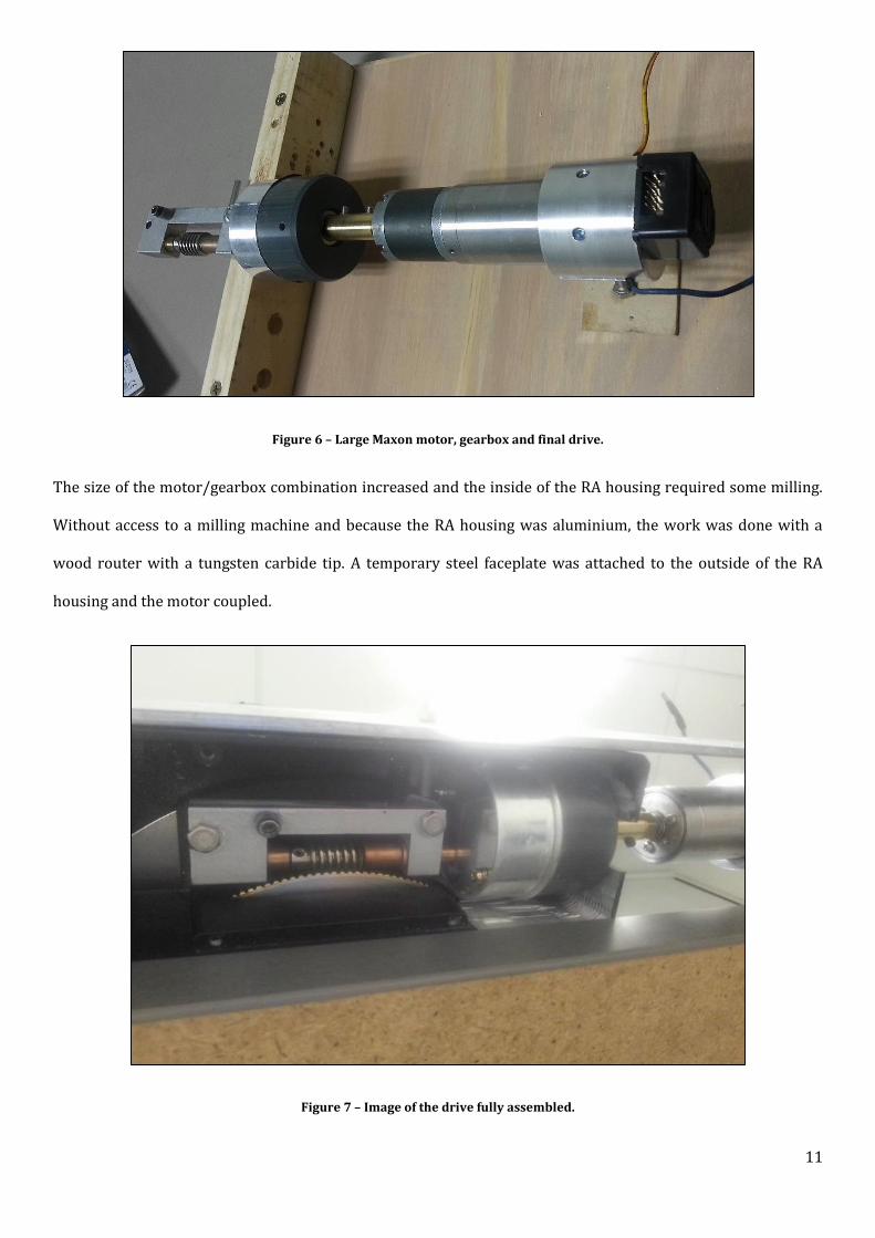
Figure 6 – Large Maxon motor, gearbox and final drive.
The size of the motor/gearbox combination increased and the inside of the RA housing required some milling.
Without access to a milling machine and because the RA housing was aluminium, the work was done with a
wood router with a tungsten carbide tip. A temporary steel faceplate was attached to the outside of the RA
housing and the motor coupled.
Figure 7 – Image of the drive fully assembled.
12
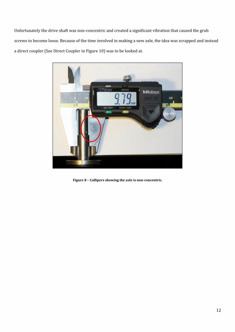
Unfortunately the drive shaft was non-concentric and created a significant vibration that caused the grub
screws to become loose. Because of the time involved in making a new axle, the idea was scrapped and instead
a direct coupler (See Direct Coupler in Figure 10) was to be looked at.
Figure 8 – Callipers showing the axle is non-concentric.
13
2.2.3 DESIGN 3
Learning from the previous motor mounting issues it was decided to purchase multiple backup motors of
varying sizes and maximum RPM’s should any future problems arise.
The gearbox axle was measured to be approximately 1.19mm (3
64") and the axle of the motor was measured to
be 3mm. The new motor had a significantly lower torque curve than the larger motor and in initial tests was
unable to overcome the inertia of the large coupler used in Design 3. Therefore a smaller coupler design was
needed.
There were no specific calculations involved for this design other than prior knowledge of shaft inertia in motor
vehicles. By lowering the moment of inertia of a spinning shaft, for a fixed power input there will be greater
acceleration but more sensitive to disturbances such as the telescope weight shifting when rotating. A larger
moment of inertia on the spinning shaft will reduce acceleration but provide a steadier supply of torque to the
final drive and thus less sensitive to disturbances. The acceleration of the shaft is not of great concern in this
application.
The coupler design would also need to be balanced to reduce vibration therefore it would have been ideal to
have the coupler fix to the shafts with 3 grub screws per side. By having the grubs spaced 120° apart the
balance of the coupler would be maintained. Unfortunately the 1.19mm shaft would not allow for this given the
lack of internal surface area and limited sizes of grub screws. Only 1 grub screw was therefore used per side
and located 180° apart. See figure below.

14
9.4mm
3mm
1.19mm
Figure 9 - Visio created image showing the basic design of the coupler
The help of John Boulton was once again employed in producing the coupler & the results of his work are
shown in Figure 10.
Figure 10 – Brass coupler from RE25 Maxon motor to old Meade gearbox.

15
The coupler worked well with only one small problem, upon start-up of the drive axis the motor would stall
until the supply voltage exceeded 5V. This was an issue because this voltage was above the calculated tracking
set-point voltage.
The problem was the grub screws were too long and were causing the moment of inertia to increase thereby
increasing the amount of starting torque required by the motor to overcome it. The image below was from
another earlier, unsuccessful build of the coupler; the grub screws sit significantly outside of the couplers
extremity.
Figure 11 – Grub screws sitting outside of coupler causing torque issues on a previous design.
Once this was discovered and the grub screws replaced with the correct sizing the starting voltage reduced to
0.7 volts and vibration was significantly reduced.
Testing of this design build was straightforward and involved confirming the motor & gearbox speed
calculations physically.
The first method was to time the motor run at a fixed voltage of 6V until the angle markings (See Figure 12) on
the telescope mount had changed by 5 degrees. The scope took 509 seconds to move 5 degrees which equated

16
to 2.36 rotations per day. The calculated value from using the gearbox ratio was 2.42 rotations per day.
Figure 12 – Image showing time/angle markings on the telescope mount.
This method was not very accurate as the markings on the mount are quite course in their resolution. However,
the method proved helpful in proving that the calculations were not grossly off.
The second method involved setting up the telescope fully and attaching a laser to the front of the optics. This
laser would then be used to track across an adjacent wall where the length would be measured after a known
time. This method would also be used as a crude visual indicator of vibration.
The scope was setup on a stable bench top which was 3.59m away from the opposite wall. The laser was then
aimed directly perpendicular to the wall and then the wall marked with pencil. The laser aim was then moved
approximately 20 cm to the side of the mark. The purpose of moving the aim was to have the path of the laser
run across the ‘flattest’ part of the wall to remove as much error in the calculation.

17
Figure 13 – Laser pointer fixed to mount to be used to calculate angular speed of mount.
A problem was encountered when testing first began. The laser would remain stagnant for a few seconds and
then rapidly move across the wall, a few centimetres, and then track steadily. This would only happen at start-
up and the issue was put down to the gearbox having a lot of slack and this was it winding up then releasing.
(The problem was later discovered to be a failing nylon gear which would slip on occasion but once moving
would operate normally.)
In order to overcome this windup during the laser testing, the motor was left to run and the telescope mounts
manual clutch engaged so the motor would take up the slack in the gearbox. After a small period of time the
clutch was disengaged and the timer was started.
The telescope moved 35.6cm in 960 seconds.
35.9𝑐𝑚
960𝑠|360°
2𝜋𝑟|
86400𝑠
𝑑𝑎𝑦= 1.42042 𝑟𝑒𝑣/𝑑𝑎𝑦
Unfortunately at the speed of rotation for the motor this should have been 2.42 rev/day as in the previous test.
The test was attempted to be repeated but the gearbox suddenly failed. This design was abandoned as the
gearbox was 20-30 years old and there would be great difficulty in finding a spare part for it.

18
2.3 TOOLS AND MACHINERY USED
Tap and Die
The tap and die set is a cutting tool used to thread the inside of drilled holes or the outside of rods. Basically
making nuts and bolts.
For this project both were used. The tap was used to make threaded holes in the couplers and motor encoder
mounts to make way for the grub screws and is known as tapping. The die was used for threading the rod
which was then used to fix the motor mount to the telescopes mount housing.
Lathe and Milling machine
The motor mounts, couplers, gearbox housing & drive shaft designs were turned on a lathe.
The motor encoder mounts, once correctly cut to size, were placed in a milling machine to take out the slots for
the motor wiring to fit.
Various
Various hand and press type drills were used for general work. The press drill was used for tapping the grub
screw holes.
A router with a tungsten carbide bit was used to ‘mill’ out the inside of the telescopes mount housing to make
way for the motor and gearbox. An angle grinder was used for cutting metal used in the temporary mounts.
Digital and vernier callipers were used for measurements of axles, thread sizes, gear tooth circular pitch and
other precise measurements.
A Dremel™ was used for small grinding and buffing on the gearbox sections and used for cutting electrical
tracks on development boards

19
Figure 15 – The Raspberry Pi Model B and 4GB
SDHC card used in the project.
3 ELECTRONIC HARDWARE
3.1 OVERVIEW
M
RA Motor
CH A,B & Z2000 cpr quadrature
AvagoH/W
Decoder8-bit BUS
Arduino Mega 2560 R3
Input = I2C BUS & 8-bit bus from Avago D ecode r
Output = PWM & I2C BUS
H-Bridge
PWM Output
Rotary Encoder 1
I 2C BU
S
RTC M
DEC Motor
Rotary Encoder 2
CH A,B & Z2000 cpr quadrature
H-Bridge
PWM Output
Output 1
Output 2
Serial
Figure 14 - Block overview of final design
3.2 RASPBERRY PI
The Raspberry Pi was launched in early 2012 just prior to the
commencement of this project. The UK based organisation,
Raspberry Pi Foundation, begun designing the boards with the
intention of using them as a teaching aid for computer science
students. (Raspberry Pi Foundation 2013)

20
The device supports many distributions of Linux including the Raspberry Pi optimised version of Debian called
Raspbian OS. (Raspbian 2012)
Using the Raspberry Pi was an addition after the project was initially discussed. There was already a demand
for a two microprocessors to handle the processing load that was to be required by the design. The additional
parts required to have an Arduino (see 3.3) perform fast Ethernet communications (~AUD$451), a USB host
controller (~AUD$302) as well as handle complex real-time calculations, becomes expensive in both currency &
system resources. The Raspberry Pi performs these functions natively using the Broadcom BCM2835 System
on Chip [SoC].
Table 3 – Specifications of the Raspberry Pi model B. (elinux.org 2013)
System on Chip (SoC) Broadcom BCM2835 CPU 700MHz ARM11 ARM1176JZF-S core GPU Broadcom VideoCore IV Memory 512MB SDRAM Expansion 2x USB2.0 Video outputs HDMI, Composite RCA Audio outputs 3.5mm stereo jack, HDMI audio Storage Secure Digital IO port Network 10/100 Ethernet - RJ45 Additional Communications SPI, 𝐼2𝐶, 𝐼2𝑆, UART, GPIO pins Real Time Clock None - Software based Power 3.5W - Max 700mA @ 5VDC Size (Metric) 85 x 56mm
1 Price sourced from SparkFun Electronics on 22/08/2013 - https://www.sparkfun.com/products/10864 2 Price sourced from SparkFun Electronics on 22/08/2013 - https://www.sparkfun.com/products/9947
21
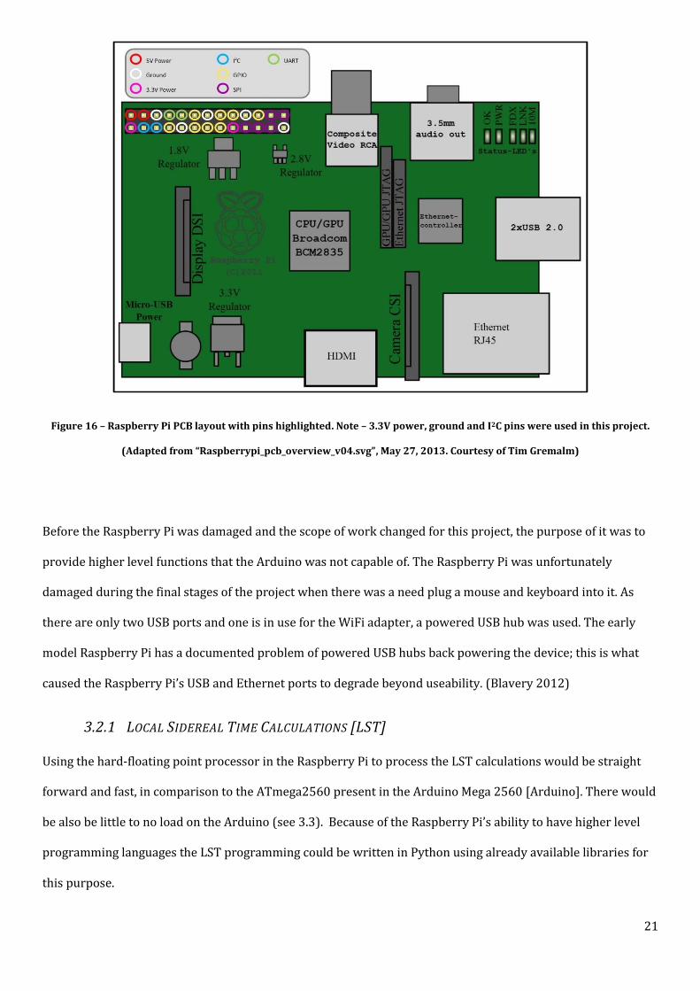
Figure 16 – Raspberry Pi PCB layout with pins highlighted. Note – 3.3V power, ground and I2C pins were used in this project.
(Adapted from “Raspberrypi_pcb_overview_v04.svg”, May 27, 2013. Courtesy of Tim Gremalm)
Before the Raspberry Pi was damaged and the scope of work changed for this project, the purpose of it was to
provide higher level functions that the Arduino was not capable of. The Raspberry Pi was unfortunately
damaged during the final stages of the project when there was a need plug a mouse and keyboard into it. As
there are only two USB ports and one is in use for the WiFi adapter, a powered USB hub was used. The early
model Raspberry Pi has a documented problem of powered USB hubs back powering the device; this is what
caused the Raspberry Pi’s USB and Ethernet ports to degrade beyond useability. (Blavery 2012)
3.2.1 LOCAL SIDEREAL TIME CALCULATIONS [LST]
Using the hard-floating point processor in the Raspberry Pi to process the LST calculations would be straight
forward and fast, in comparison to the ATmega2560 present in the Arduino Mega 2560 [Arduino]. There would
be also be little to no load on the Arduino (see 3.3). Because of the Raspberry Pi’s ability to have higher level
programming languages the LST programming could be written in Python using already available libraries for
this purpose.

22
3.2.2 CONNECTIVITY
The Raspberry Pi has built in Ethernet and the ability to support a USB WiFi dongle. This would have allowed
the device to be housed alongside the Arduino on the roof of the engineering building and still be connectable.
The Raspberry Pi was configured to host a basic website that streamed a webcam feed live over HTTP that
supported multiple viewers at once.
3.2.3 PHOTOGRAPHY
There are two methods of photography that were researched, the Digital SLR camera and a dedicated CCD
camera.
The Schmidt-Cassegrain (Linfoot 1956) telescope allows a Digital SLR [DSLR] camera to be easily fixed to the
eye piece with an adapter. The Raspberry Pi was to use an open-source software package, called Entangle, to
send commands to the camera to take long exposures when the telescope was in sidereal tracking. (Berrangé
2012)
Entangle can be used interactively and has a well-developed user interface and is simple to use and configure.
The software allows the use of text based scripts which can be used to run the software via command line and
this feature was to later be used to adjust the settings when tracking different celestial objects. (Starizona
2013)
Once images were taken with either solution, the Raspberry Pi could then facilitate the transfer of the images to
a Murdoch University shared drive where the images can then be viewed.
Advantages of DSLR – Second hand or budget DSLR cameras are
very cheap due to being mass produced. They can also be used for
normal photography when not being used for astrophotography.
Disadvantages of DSLR – Bulky, may not be able to be left in situ,
cheaper models may not be as sensitive to light as a dedicated
astrophotography CCD sensor such as the one shown in Figure 17.
Figure 17 – USB CCD attached to telescope with
filter wheel (Courtesy of Marie-Lan Nguyen
2007)

23
Advantages of USB CCD – Widely supported by software for astrophotography. Faster imaging and
USB connectivity. Small form and can be left in situ. Can be used for tracking error correction with
certain software.
Disadvantages of USB CCD – Often costly depending on quality. Software can be expensive.
3.3 ARDUINO MICROCONTROLLER
Once again, avoiding proprietary hardware was a hard constraint in this project as the associated software
often requires licensing and the hardware is expensive to replace. An example of such products are
Programmable Logic Controllers or Data Acquisition devices; both very capable products yet can be very
expensive.
This hard constraint left only open source hardware available for the project; thankfully there is a multitude of
options on the market due to the increased power of microelectronics coupled with the reduction in
manufacturing.
Many of these options have been widely adopted by electronic enthusiasts but, many would argue, only one
development board manufacturer truly stands out in terms of price, availability, maturity, quality, support &
direction; Arduino. (Google Trends 2013; Torrone 2011)
The Arduino project begun in Italy in 2005. The founders of the project intended to build a prototyping board
that was less expensive than the current market offerings that could be used by students in design projects.
Since being founded the company has commercially produced 16 boards of which all but one have been based
on the 8bit megaAVR microcontroller; the most recent, the Arduino Deu, is based on the 32bit Amtel ARM
Cortex-M3 microcontroller. (Arduino 2013)
The Arduino Mega 2560 R3 development board is at the heart of this project. The board offers a multitude of
inputs, outputs and timers, all of which are heavily used within the project. (Arduino 2013)

24
Figure 18– Arduino Mega2560
Table 4 – list of Arduino Mega 2560 R3 features
Feature Number Resolution Digital Input/Output 54 multi-purpose pins - Analog Inputs 16 10bit External hardware interrupts 6 - PWM out 14 8bit 𝐼2𝐶 1 pair - Serial 4 pairs - SPI 1 -
3.3.1 TIMERS
The Arduino Mega 2560 R3 has 6 hardware timers (Arduino 2013) in total and attached to each timer is a
counter which increments with every tick of their associated timer. Each timer is attached to the Arduino’s
16MHz processor via a pre-scaling register. A 1:1 pre-scalar would increment the given timers counter by 1
each cycle of the processor, or every 62.5ns; 1024:1 pre-scalar would increment the counter every 64µs.
These timers and counters handle anything from generating PWM frequencies, configuring hardware
interrupts and also used for timer overflow functions. (Arduino 2013); (Ghassaei 2012).
The PWM generation is used in this project to provide the motors with a fast PWM signal which is suitable for
driving motors of this specification. (See 3.7.1)
25
In earlier designs, hardware interrupts were going to be used to trigger events within the software and to
capture the number of ticks of the rotary encoder. This function was later offloaded to the hardware decoder.
(See 3.6.2)
Another function of the timers is the Clear Timer on Compare [CTC]. When a timer’s counter reaches a value,
programmed into the register, the counter will overflow and provide a hardware interrupt which can be used
for time critical applications. This register was used for triggering the PID controller to perform measurements
and calculations every 50ms. (see 4.2.1)
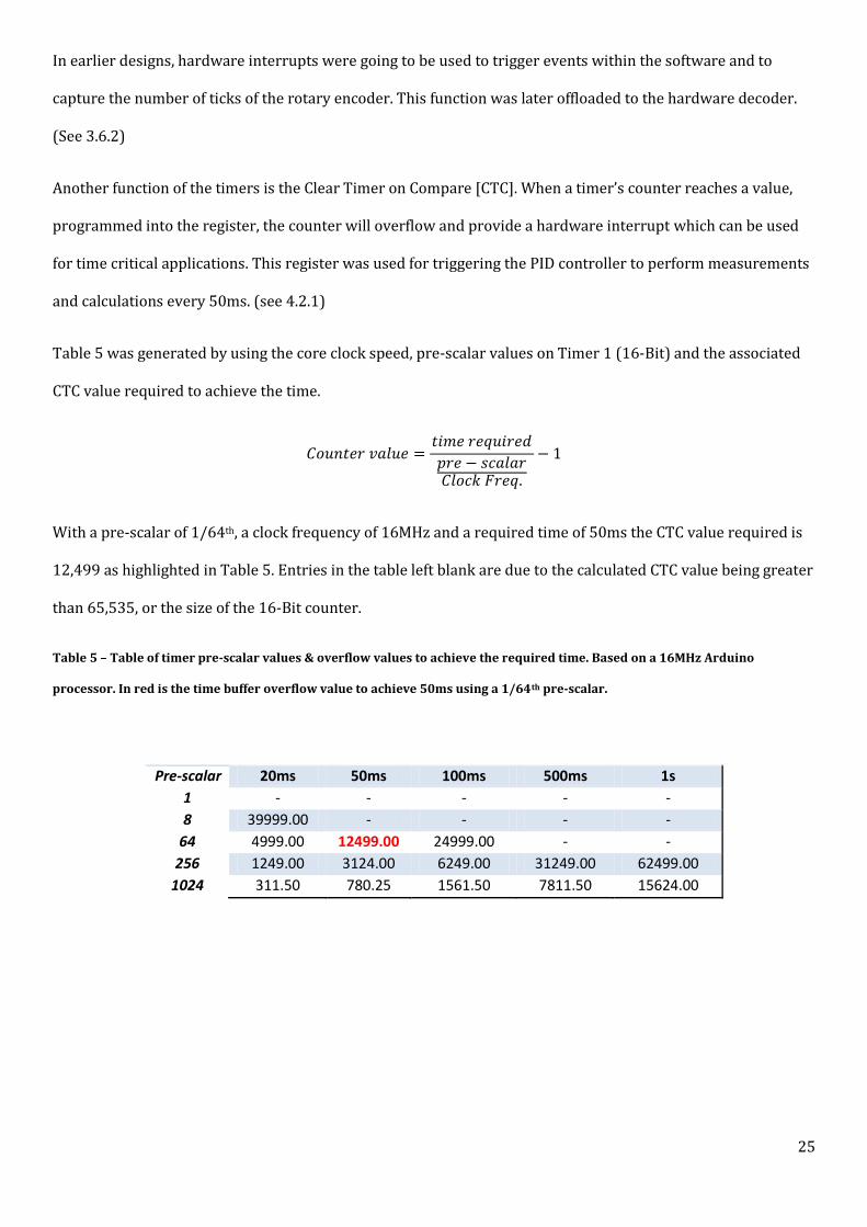
Table 5 was generated by using the core clock speed, pre-scalar values on Timer 1 (16-Bit) and the associated
CTC value required to achieve the time.
𝐶𝑜𝑢𝑛𝑡𝑒𝑟 𝑣𝑎𝑙𝑢𝑒 =𝑡𝑖𝑚𝑒 𝑟𝑒𝑞𝑢𝑖𝑟𝑒𝑑
𝑝𝑟𝑒 − 𝑠𝑐𝑎𝑙𝑎𝑟𝐶𝑙𝑜𝑐𝑘 𝐹𝑟𝑒𝑞.
− 1
With a pre-scalar of 1/64th, a clock frequency of 16MHz and a required time of 50ms the CTC value required is
12,499 as highlighted in Table 5. Entries in the table left blank are due to the calculated CTC value being greater
than 65,535, or the size of the 16-Bit counter.
Table 5 – Table of timer pre-scalar values & overflow values to achieve the required time. Based on a 16MHz Arduino
processor. In red is the time buffer overflow value to achieve 50ms using a 1/64th pre-scalar.
Pre-scalar 20ms 50ms 100ms 500ms 1s
1 - - - - -
8 39999.00 - - - -
64 4999.00 12499.00 24999.00 - -
256 1249.00 3124.00 6249.00 31249.00 62499.00
1024 311.50 780.25 1561.50 7811.50 15624.00
26
3.4 REAL TIME CLOCK
The Maxim Integrated DS1307 Real Time Clock [RTC] (maxim integrated 2011) was chosen for this project due
to its price, availability and ability to talk over an I2C bus. The RTC is a critical piece of hardware if the telescope
were to be used offline because it provides the Arduino software the means of calculating the Local Sidereal
Time.
The DS1307 also provides a programmable square wave output which can be used as a trigger for a hardware
interrupt, and 56 Bytes of storage which can be written to over the 𝐼2𝐶 bus. This memory has been used to
store telescope positional information should the Arduino lose power. The benefit of storing information on the
DS1307 is that it has an incredibly low power consumption, which means its Lithium Ion battery backup lasts
approximately 10 years.
The 8 pin IC is also very small form factor and even when fully assembled it can be safely mounted on the pin
headers of the Arduino Mega 2560.
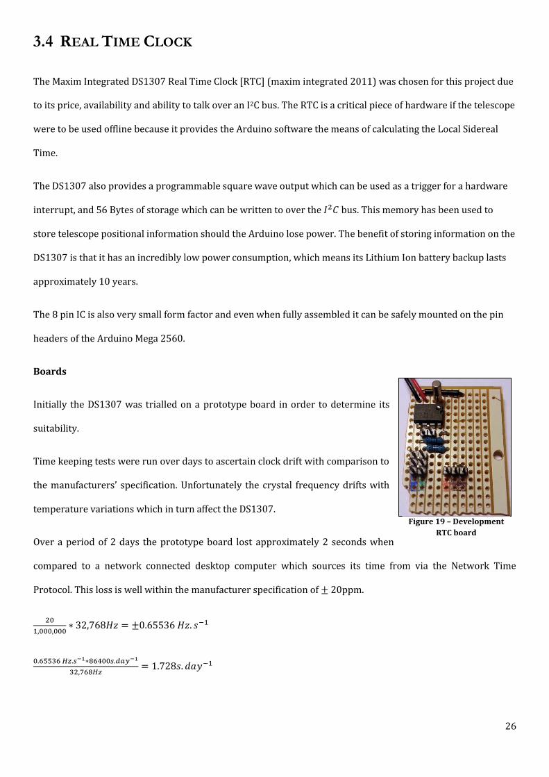
Boards
Initially the DS1307 was trialled on a prototype board in order to determine its
suitability.
Time keeping tests were run over days to ascertain clock drift with comparison to
the manufacturers’ specification. Unfortunately the crystal frequency drifts with
temperature variations which in turn affect the DS1307.
Over a period of 2 days the prototype board lost approximately 2 seconds when
compared to a network connected desktop computer which sources its time from via the Network Time
Protocol. This loss is well within the manufacturer specification of ± 20ppm.
20
1,000,000∗ 32,768𝐻𝑧 = ±0.65536 𝐻𝑧. 𝑠−1
0.65536 𝐻𝑧.𝑠−1∗86400𝑠.𝑑𝑎𝑦−1
32,768𝐻𝑧= 1.728𝑠. 𝑑𝑎𝑦−1
Figure 19 – Development
RTC board
27
While this rate is acceptable for tracking and positioning within the same day,
over multiple days the accuracy of the scope to slew to a target will be
considerably off. Therefore the solution is to have the Raspberry Pi update the
clock via the Network Time Protocol time on a schedule it receives from the
university network routers. (Network Time Foundation n.d.)
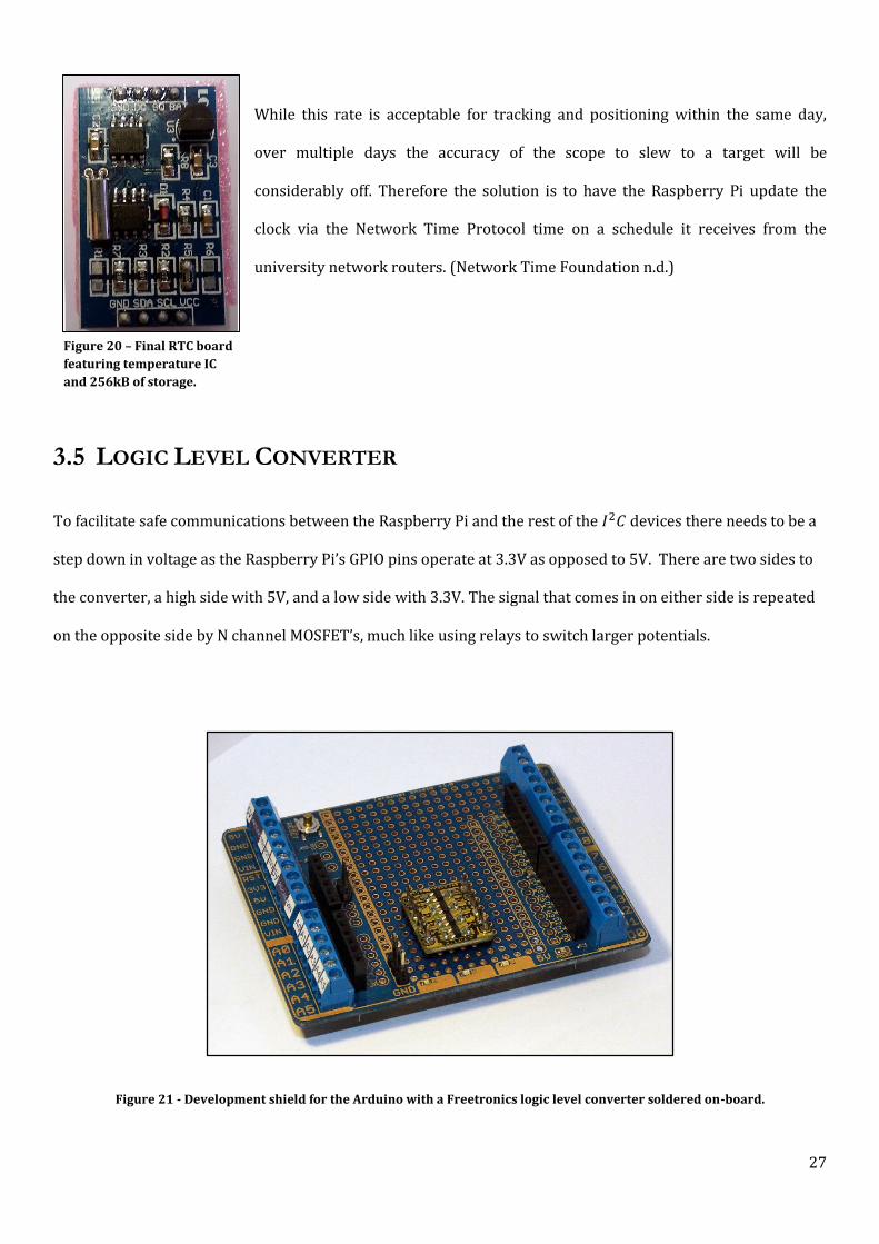
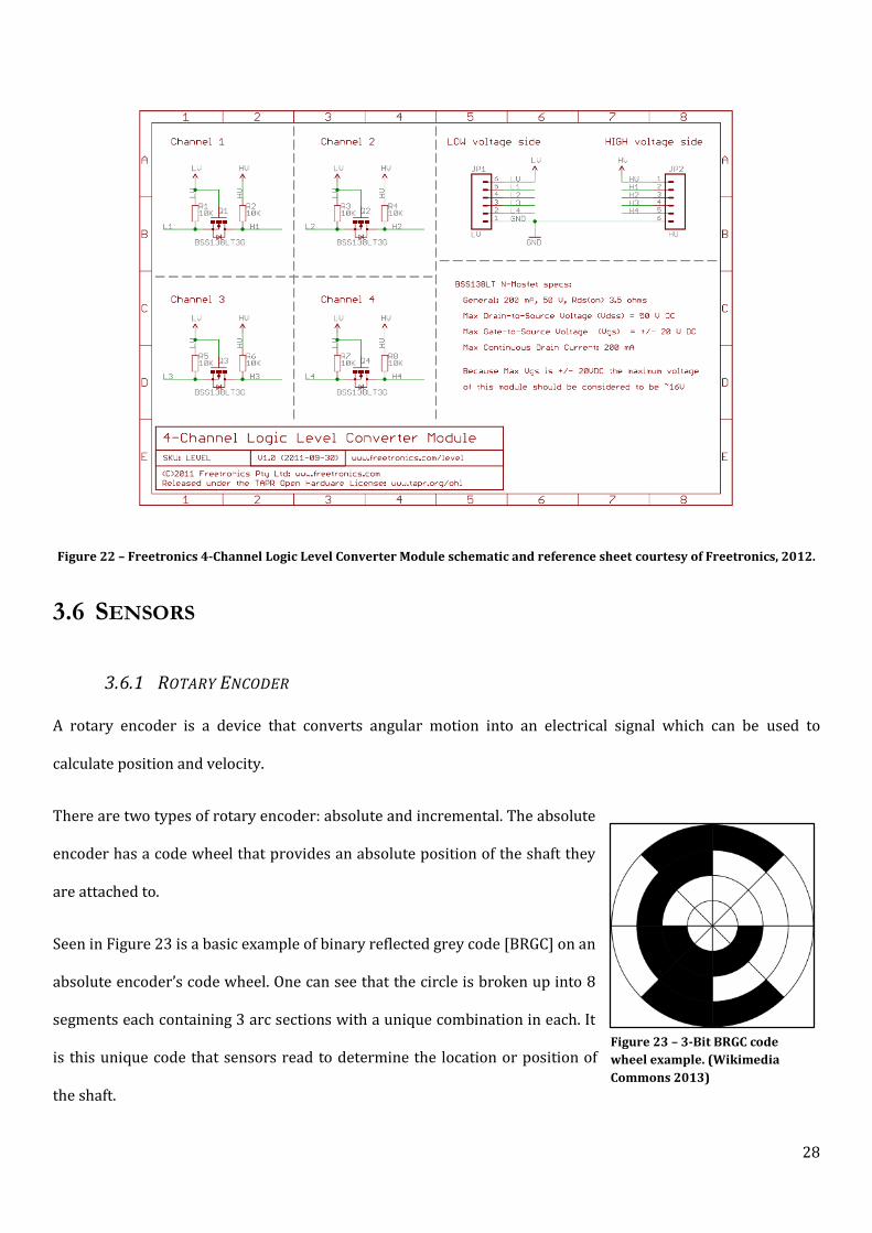
3.5 LOGIC LEVEL CONVERTER
To facilitate safe communications between the Raspberry Pi and the rest of the 𝐼2𝐶 devices there needs to be a
step down in voltage as the Raspberry Pi’s GPIO pins operate at 3.3V as opposed to 5V. There are two sides to
the converter, a high side with 5V, and a low side with 3.3V. The signal that comes in on either side is repeated
on the opposite side by N channel MOSFET’s, much like using relays to switch larger potentials.
Figure 21 - Development shield for the Arduino with a Freetronics logic level converter soldered on-board.
Figure 20 – Final RTC board
featuring temperature IC
and 256kB of storage.
28
Figure 22 – Freetronics 4-Channel Logic Level Converter Module schematic and reference sheet courtesy of Freetronics, 2012.
3.6 SENSORS
3.6.1 ROTARY ENCODER
A rotary encoder is a device that converts angular motion into an electrical signal which can be used to
calculate position and velocity.
There are two types of rotary encoder: absolute and incremental. The absolute
encoder has a code wheel that provides an absolute position of the shaft they
are attached to.
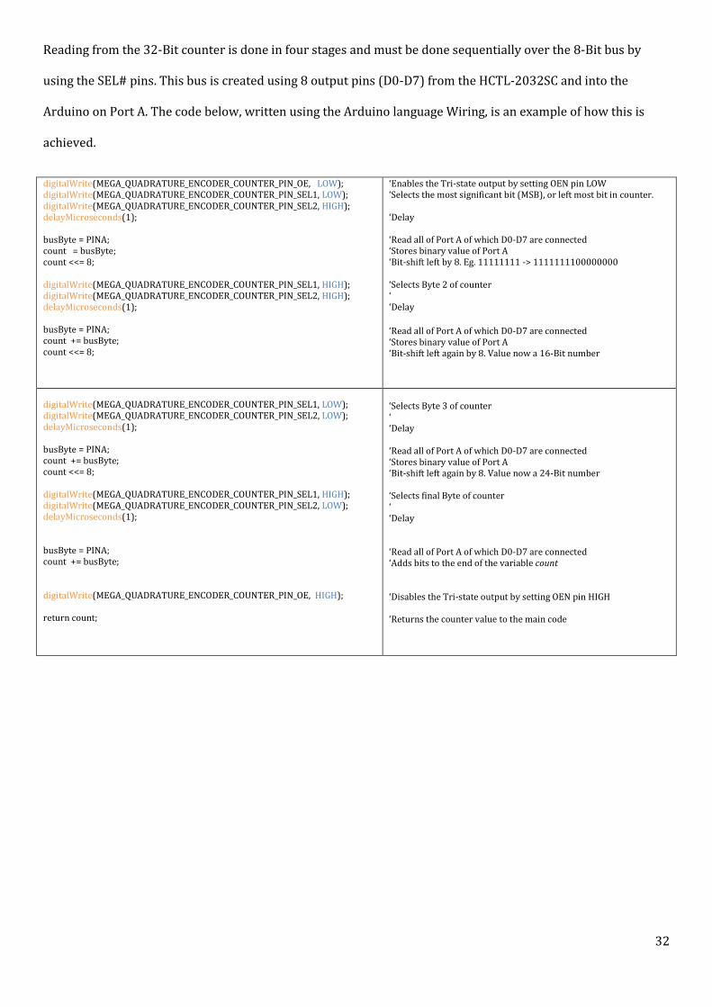
Seen in Figure 23 is a basic example of binary reflected grey code [BRGC] on an
absolute encoder’s code wheel. One can see that the circle is broken up into 8
segments each containing 3 arc sections with a unique combination in each. It
is this unique code that sensors read to determine the location or position of
the shaft.
Figure 23 – 3-Bit BRGC code
wheel example. (Wikimedia
Commons 2013)

29
This example is a 3-Bit code wheel and provides a rather large 45° of uncertainty. By increasing the number of
rings on the code wheel the level of uncertainty can be reduced and the resolution increased. For ‘n’ of rings the
segment number is 2𝑛. E.g. 16-Bit would equate to 65536 segments or an angle of 0.0055°.
The incremental rotary encoder is a relative type sensor which provides a rate of change, or speed, of the shafts
rotation. This is achieved, in this example, by using an optical sensor and wheel with notches taken out. When
the notches pass over the optical sensor a high pulse is registered on its output and when the optical sensor is
covered a low is detected. By counting the number of pulses per second an angular velocity can be determined.
Similar to the absolute encoder, by increasing the number of notches the angular resolution can be increased
directly. Furthermore, by adding another sensor that is offset to the first sensor, by counting both rising and
falling edges of each sensor the resolution can be increased by a factor of 4. This is known as quadrature mode.
Unfortunately incremental encoders have drawbacks if they are used for anything other than speed
measurements, such as having to be constantly monitored if the control system accurately wants to know the
location of the shaft, unlike the absolute encoder.
Figure 24 – Example of rotary encoder wheel courtesy of Rrudzik, 2011.
The ultimate instrument for this project would have been an absolute optical rotary encoder which sat directly
on the mount which would give an ‘absolute’ position with extreme resolution. Renishaw RESOLUTE encoders
were the range of products that had a resolution of 27 Bits, are absolute and came in multiple ring sizes which
would sit directly on the final drive; unfortunately the prices started around $4,000 USD. (Reinshaw n.d.)
Another method of achieving this high resolution was to have the encoder placed at the fastest spinning
location in the system rather than the final drive, or even step up the speed. This would allow for a less accurate
encoder but because each pulse would equate to a much smaller angular change of the final drive the resolution
would be increased.

30
With a limited budget and a requirement for high resolution it was decided to go with the less accurate encoder
placed at the fastest location, the rear of the motor. Another consideration was the drive shaft size and
extrusion from the motor assembly because the encoder would need to be secured to it. The drive shaft is 6mm
dia. and extruded 18mm.
Two manufacturers stood out due to their popularity in robotics; US Digital & Avagotech.
Both manufacturers allowed custom configuration (bore, resolution, output type, index gating, mounts) of their
encoders. US Digital offered little support and were not stocked locally; the decision was made to go with
Avagotech who were supplied by major Australian suppliers.
The encoders that were chosen for this project were the Avago HEDS-5540, 2
channel quadrature output with 500 cycles per revolution [CPR] of the disc.
CPR is the number of cycles the encoder will go through for every full rotation
of the code-wheel. The CPR is a measure of resolution which is very important
in this application because, the more resolution that is available, the more
accurate the feedback controller will be and in turn the sidereal tracking.
The large motors maximum speed is 2800RPM and the total ratio of the
gearboxes is 378,000:1.
What this equates to is that for every 1° of slew of the mount the motor will
have revolved 1050 times.
378,000 [𝑟𝑒𝑣𝑚𝑜𝑡𝑜𝑟𝑟𝑒𝑣𝑚𝑜𝑢𝑛𝑡
]
360 [𝑑𝑒𝑔
𝑟𝑒𝑣𝑚𝑜𝑢𝑛𝑡]
= 1050 [𝑟𝑒𝑣𝑚𝑜𝑡𝑜𝑟
𝑑𝑒𝑔]
As sidereal tracking is required in order to take astrophotography the motor accuracy needs to be fine. The
500CPR encoder produces 2000 pulses per rotation (PPR).
This gives the current configuration a theoretical resolution of 4.76191𝐸 − 07 ° {5dp}.
Figure 25 – Avago HEDS-5540

31
The Renishaw absolute encoder had 27 Bits of resolution which equates to 7.4506𝐸 − 09° {4𝑑𝑝}. This makes
the Renishaw approx. 60x more accurate at the final drive, yet 70x more expensive at a minimum.
3.6.2 BINARY COUNTER
In order to count the pulses of the rotary encoder without
having a severe impact on the Arduino, a binary counter has
been used. The HCTL-2032-SC, as pictured in Figure 26, was
the CMOS IC used in this project. (Avago Tech 2013)
The purpose of the counter was to remove the requirement of
the Arduino to use its hardware interrupt timers to count the
pulses of the rotary encoders due to the large number of pulses
that would be generated at full speed of the motors. The HCTL-2032-SC provides two 32-Bit counters, a
quadrature decoder, index support, digital filters with high noise immunity and easy communications via an 8-
Bit Tristate bus.
The IC had already been developed into a shield for the Arduino and was purchased pre-manufactured and
supplied with an already developed library. This library has been heavily used in the programming of the
Arduino.
Figure 27 – Information on how to select which byte is read from the counter. (Avago Tech 2013)
Figure 26 – Avago HCTL-2032SC binary counter
on a Robogaia counter shield.
32
Reading from the 32-Bit counter is done in four stages and must be done sequentially over the 8-Bit bus by
using the SEL# pins. This bus is created using 8 output pins (D0-D7) from the HCTL-2032SC and into the
Arduino on Port A. The code below, written using the Arduino language Wiring, is an example of how this is
achieved.
digitalWrite(MEGA_QUADRATURE_ENCODER_COUNTER_PIN_OE, LOW); digitalWrite(MEGA_QUADRATURE_ENCODER_COUNTER_PIN_SEL1, LOW); digitalWrite(MEGA_QUADRATURE_ENCODER_COUNTER_PIN_SEL2, HIGH); delayMicroseconds(1); busByte = PINA; count = busByte; count <<= 8; digitalWrite(MEGA_QUADRATURE_ENCODER_COUNTER_PIN_SEL1, HIGH); digitalWrite(MEGA_QUADRATURE_ENCODER_COUNTER_PIN_SEL2, HIGH); delayMicroseconds(1); busByte = PINA; count += busByte; count <<= 8;
‘Enables the Tri-state output by setting OEN pin LOW ‘Selects the most significant bit (MSB), or left most bit in counter. ‘Delay ‘Read all of Port A of which D0-D7 are connected ‘Stores binary value of Port A ‘Bit-shift left by 8. Eg. 11111111 -> 1111111100000000 ‘Selects Byte 2 of counter ‘ ‘Delay
‘Read all of Port A of which D0-D7 are connected ‘Stores binary value of Port A ‘Bit-shift left again by 8. Value now a 16-Bit number
digitalWrite(MEGA_QUADRATURE_ENCODER_COUNTER_PIN_SEL1, LOW); digitalWrite(MEGA_QUADRATURE_ENCODER_COUNTER_PIN_SEL2, LOW); delayMicroseconds(1); busByte = PINA; count += busByte; count <<= 8; digitalWrite(MEGA_QUADRATURE_ENCODER_COUNTER_PIN_SEL1, HIGH); digitalWrite(MEGA_QUADRATURE_ENCODER_COUNTER_PIN_SEL2, LOW); delayMicroseconds(1); busByte = PINA; count += busByte; digitalWrite(MEGA_QUADRATURE_ENCODER_COUNTER_PIN_OE, HIGH); return count;
‘Selects Byte 3 of counter ‘ ‘Delay ‘Read all of Port A of which D0-D7 are connected ‘Stores binary value of Port A ‘Bit-shift left again by 8. Value now a 24-Bit number ‘Selects final Byte of counter ‘ ‘Delay ‘Read all of Port A of which D0-D7 are connected ‘Adds bits to the end of the variable count ‘Disables the Tri-state output by setting OEN pin HIGH ‘Returns the counter value to the main code
33
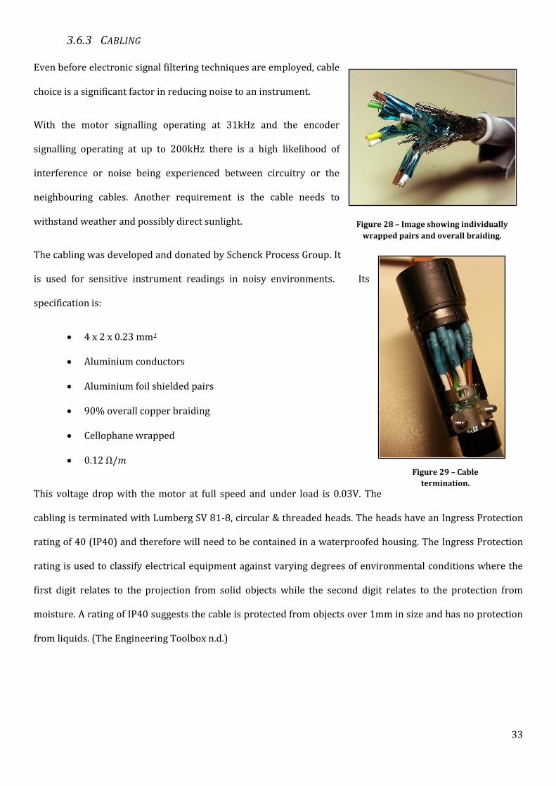
Figure 29 – Cable
termination.
3.6.3 CABLING
Even before electronic signal filtering techniques are employed, cable
choice is a significant factor in reducing noise to an instrument.
With the motor signalling operating at 31kHz and the encoder
signalling operating at up to 200kHz there is a high likelihood of
interference or noise being experienced between circuitry or the
neighbouring cables. Another requirement is the cable needs to
withstand weather and possibly direct sunlight.
The cabling was developed and donated by Schenck Process Group. It
is used for sensitive instrument readings in noisy environments. Its
specification is:
4 x 2 x 0.23 mm2
Aluminium conductors
Aluminium foil shielded pairs
90% overall copper braiding
Cellophane wrapped
0.12 Ω/𝑚
This voltage drop with the motor at full speed and under load is 0.03V. The
cabling is terminated with Lumberg SV 81-8, circular & threaded heads. The heads have an Ingress Protection
rating of 40 (IP40) and therefore will need to be contained in a waterproofed housing. The Ingress Protection
rating is used to classify electrical equipment against varying degrees of environmental conditions where the
first digit relates to the projection from solid objects while the second digit relates to the protection from
moisture. A rating of IP40 suggests the cable is protected from objects over 1mm in size and has no protection
from liquids. (The Engineering Toolbox n.d.)
Figure 28 – Image showing individually
wrapped pairs and overall braiding.

34
3.7 RIGHT ASCENSION DRIVE
The very early project specification had three accurate stepper motors to drive the 3 axes. Stepper motors have
high torque at low speeds and high holding torque, which was attractive given the extremely low speeds that
would be required for sidereal tracking.
The plan was to micro-step the motors in order to increase resolution. That is, rather than stepping the motor
between the discrete positions of the coils, to charge multiple coils to create a new point of magnetic
equilibrium that the rotor turns to. This is achieved by providing the phases of the motor with sinusoidal input
functions rather than a Heaviside step function. It was soon determined that a 0.9° step with 10 microsteps
would need 4000 operations from the Arduino per revolution, per motor. (Machine Tool Help 2010)
Figure 30 – One phase, 1 Hz sinusoid with its micro-step approximation in comparison to full steps.
The initial response to this issue was to look at dedicated stepper motor drivers with encoder feedback loops
inbuilt. (Robokits n.d.) Unfortunately this was expensive so the idea was dropped and replaced with an H-
Bridge driven synchronous motor setup.
There were two motors that were specified for this project due to the mechanical failures. Specifications of each
are listed below.

35
Table 6 - Maxon 34mm - 2434.970 53.225-200 – Motor specifications
Manufacturer Spec. Measured. Spec Voltage Max DC - 24V Current Max - 0.44A – no load Winding Resistance - 1.98Ω Winding Inductance - 0.62 mH Time Constant - 3.13 𝜇𝑠
Table 7 – Maxon RE25 PN 118743 - Motor specifications
Manufacturer Spec. Measured. Spec Voltage Max DC 12V - Current Max 1.2A - Winding Resistance 2.12Ω 2.12Ω Winding Inductance 0.238 mH 0.281 mH Time Constant 1.092𝜇𝑠 1.3255 𝜇𝑠
3.7.1 PULSE WIDTH MODULATION
Driving the motor at the correct speed requires the voltage be controlled accurately. Linear voltage regulators
offer this accuracy but at a heavy efficiency cost. (MIT 2000)
Pulse Width Modulation offers a greater efficiency without losing accuracy, if configured correctly for the
application. PWM works by issuing a series of pulses and adjusting the width of the pulse to vary the R.M.S.
voltage.
Figure 312 – Large Maxon motor with encoder mount and
gearhead fixed.
Figure 321 – Large Maxon motor with
gearhead removed for fixing to another old
gearbox.

36
Figure 33 – Varying duty cycle of a PWM output on an Arduino. Courtesy of Arduino.cc team, 2010.
Additional motor heating occurs at very low PWM frequencies, compared to a pure DC supply, due to the
discontinuity of the current flow. The motor’s inductance & inertia do not store enough energy to maintain a
steady current waveform during the PWM’s off period. This is known as ripple current and as it increases so
does the motor heating. The way to mitigate this problem is to make certain that the PWM’s pulse frequency is
smaller than the motor’s time constant.
The Maxon RE25 time constant is 1.3255𝜇𝑠. A PWM frequency for a specified duty cycle can be determined by
using working out the time constant of the motor inductance and resistance values measured.
𝑃𝑊𝑀 = (2𝐿𝑚
𝑅𝑚)
−1
∗1
𝐷𝑢𝑡𝑦 𝐶𝑦𝑐𝑙𝑒
For instance the Maxon RE25 motor, when tracking, operates at 30% duty cycle then the following PWM
frequency is recommended at a minimum.
𝑃𝑊𝑀 = (2 ∗0.234𝑚𝐻
2.18Ω)
−1
∗1
0.3
𝑃𝑊𝑀 = 15527.1 𝐻𝑧

37
Testing
The performance of the PID controller (discussed in 4.2.1) was measured at different PWM frequencies to
determine which was best at holding set point after a 0-34% step was made. As the Arduino only has a fixed
number of frequencies only three were tested; 976 Hz, 3.9 kHz & 31.25 kHz.
Figure 34 – MV & PV variance and PID controller effort required when operating PWM at 976Hz.
0
5
10
15
20
25
30
35
40
45
50
0 2 4 6 8 1 0 1 2 1 4
PV
& M
V %
TIME IN SECONDS
976HZ PWM - SET POINT STEP 0-34%
PV Adj. MV Adj.

38
Figure 35 – MV & PV variance and PID controller effort required when operating PWM at 3.9kHz.
Figure 36 – MV & PV variance and PID controller effort required when operating PWM at 31.25kHz.
0
5
10
15
20
25
30
35
40
45
50
0 2 4 6 8 1 0 1 2 1 4
PV
& M
V A
CTI
ON
%
TIME IN SECONDS
3.9KHZ PWM - SET POINT STEP 0-34%
PV Adj. MV Adj.
0
5
10
15
20
25
30
35
40
45
50
0 2 4 6 8 1 0 1 2 1 4
PV
& M
V %
TIME IN SECONDS
31.25KHZ PWM - SET POINT STEP 0-34%
PV Adj. MV Adj.

39
By summing & squaring the deviation from the set point a somewhat crude performance score can be used to
determine the best PWM frequency for set point tracking. Seen below are the final residual sum of squares
scores with the 31.25 kHz PWM frequency best suited for this project.
𝑅𝑆𝑆976𝐻𝑧 = 1,215,595
𝑅𝑆𝑆3.9𝑘𝐻𝑧 = 402,548
𝑅𝑆𝑆31.24𝑘𝐻𝑧 = 278,536
Table 8 – Experimentally captured data from Oscilloscope using the rotary encoder index pin and comparing the results to the
Arduino calculated RPM values.
Voltage Current Oscilloscope
Index Freq. (Hz)
Oscilloscope inferred
RPM
Calculated RPM
Error %Error
14.971 0.07 100.405 6024.3 6020 4.3 0.07%
14.039 0.07 94.07 5644.2 5640 4.2 0.07%
12.992 0.07 86.9 5214 5211 3 0.06%
11.937 0.07 79.79 4787.4 4776 11.4 0.24%
10.865 0.06 72.55 4353 4345 8 0.18%
9.279 0.09 61.58 3694.8 3682 12.8 0.35%
7.861 0.08 52.15 3129 3125 4 0.13%
5.826 0.06 38.5 2310 2309 1 0.04%
4.926 0.07 32.47 1948.2 1950 -1.8 -0.09%
4.1219 0.07 27.17 1630.2 1622 8.2 0.50%
3.0798 0.06 20.07 1204.2 1203 1.2 0.10%
2.4625 0.08 15.77 946.2 945 1.2 0.13%
y = 404.83x - 50.872R² = 1
0
1000
2000
3000
4000
5000
6000
7000
0 2 4 6 8 10 12 14 16
RP
M
VOLTAGE (V)
LINEAR RELATIONSHIP OF VOLTAGE & RPM
Calculated RPM Linear (Calculated RPM)
Figure 37 – Highly linear relationship of Voltage input and angular velocity of the
motor.

40
4 SOFTWARE DEVELOPMENT
4.1 RASPBIAN OS
Raspbian OS is an unofficial operating system, based on Debian Linux distribution. Raspbian OS is a fork of
Debian “wheezy” modified for the ARMv6 architecture, with its kernel sourced from a similar ARM processor
architecture. Debian “wheezy” is dubbed ‘soft-float’ as it uses the processor integer registers for its floating
point calculations. On the other hand, Raspbian OS fully supports the on-board vector floating point (VFP)
registers and thus is dubbed ‘hard-float’. (Raspbian 2012)
The benefit of having the VFP registers handle the floating point arithmetic is the speed at which they process.
In a blog article (3drenderblog 2012), a test was conducted in which the experimenter saw an 2.5x increase in
rendering performance from using Raspbian ‘hard-float’ operating system over Debian ‘soft-float’. Also in a
more recent study which included matrix manipulations of a 100x100 matrix there was up-to a 6x decrease in
execution time when using Raspbian OS. (trouch 2013)
Before the Raspberry Pi was damaged and the scope of work changed for this project, the purpose of it was to
provide higher level functions that the Arduino wasn’t capable of. It was to provide a separation between the
real time processing environment on the Arduino and the user interface.
Design
Steps that took place during the Raspberry Pi development. Full tutorials can be found in the appendices.
Build the OS – Raspbian OS.
Install ‘freerdp-x11’ to allow remote desktop support from an MS Windows based computer.
Install ‘Motion’ for webcam server to be later used for live viewing or spotter scope view.
Compile ‘Entangle’ from source code to be used with digital camera for photography.
Setup 𝐼2𝐶 to talk directly to the DS1307+ and Arduino
o Install logic level converter 3.3V <-> 5V
o Modify GPIO configurations to allow I2C to start on the Raspberry Pi

41
o Set Raspberry Pi as master with RTC and Arduino as slave
o Change Raspbian OS to retrieve time from hardware clock rather than the default software
clock.
Use already available Python based Local Sidereal Time libraries for tracking calculations. (New Mexico
Tech 2010)
Figure 38 – Remote desktop from a Windows 7 based computer displaying the terminal on the Raspberry Pi.
42
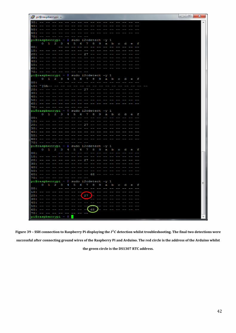
Figure 39 – SSH connection to Raspberry Pi displaying the 𝑰𝟐𝑪 detection whilst troubleshooting. The final two detections were
successful after connecting ground wires of the Raspberry Pi and Arduino. The red circle is the address of the Arduino whilst
the green circle is the DS1307 RTC address.

43
Figure 40 – The Raspberry Pi serving a live display of webcam over HTTP. The webcam will serve live images from the
telescope to multiple users over TCP/IP.
44
4.2 ARDUINO PROGRAMMING
The Arduino adopts a variant of the programming language C++, known as Wiring. It is an open source
framework that was developed in 2003 specifically for microcontrollers.
The development of this project was done directly in the Arduino IDE or in Visual Studio 2008 Professional
with a purchased add-on called Visual Micro. (Arduino 2012); (Visual Micro Limited 2013)
Visual Micro offers online syntax suggestions and a higher level of debugging than can be achieved with the
standard Arduino IDE. Within the debugging environment breakpoints are extremely useful to determine
which code is being run, and the debugger also includes live variable monitoring. If a variable needed to be
monitored, within the Arduino IDE, the easiest solution would be to output the variable to the serial interface
and read it from there.
4.2.1 PROPORTIONAL, INTEGRAL & DERIVATIVE (PID) CONTROLLER
The PID controller was initially developed using the discrete time velocity form and setup using interrupts.
𝑚2 = 𝑚1 + 𝐾𝑐 ((1 +Δ𝑡
𝜏𝑖+
𝜏𝑑
Δ𝑡) ε0 − (1 −
2𝜏𝑑
Δt) ε1 +
𝜏𝑑
Δtε0 )
The benefit of using the velocity form is the inherent anti-reset-windup property that exists within it, that does
not allow previous error to build up infinitely, thereby creating large MV movements.
Later it was discovered that a PID library had already been developed which was then tested and deemed
feasible. The PID V1.01 library, available to download from the Arduino library section, is free to use under the
GPLv3 License. (Beauregard 2012)

45
Zeigler-Nichols Stability Margin Controller Tuning
The Zeigler-Nichols [Z-N] tuning method has been used in this project due to its simplicity. Basically the
method involves closing the loop around the process variable, namely the motor RPM, with a proportional-only
controller. The gain of the controller is then increased in stages, each time stepping the motor. As the motor is a
higher order system with some lag there will be a point of instability where the system begins to oscillate. This
point is known as the ‘ultimate controller gain’ or 𝐾𝐶𝑈. (Ogunnaike and Ray 1994)
Once 𝐾𝐶𝑈 has been reached the period of oscillation is measured; 𝑃𝑈.
These values are entered into the below formula and controller parameters are returned.
Table 9 - Ziegler-Nichols Stability Margin Controller Tuning Parameters. (Ogunnaike and Ray 1994)
𝑲𝑪 𝝉𝒊 𝝉𝒅 P 0.5𝐾𝐶𝑈 - - PI 0.45𝐾𝐶𝑈 𝑃𝑈
1.2
-
PID 0.6𝐾𝐶𝑈 𝑃𝑈
2
𝑃𝑈
8
0
500
1000
1500
2000
0 0.5 1 1.5 2 2.5 3
ENC
OD
ER T
ICK
S O
N M
OTO
R
TIME IN SECONDS
Z-N - MARGINAL TUNING
Process Variable Manipulated Variable
Figure 41- Results of ZN stability margin analysis. The period of oscillation was measured, by determining the peak
to peak time. This is illustrated with two arrows in the figure.

46
Period Ultimate of 130ms with a controller gain of 0.101.
Table 10 – Ziegler-Nichols calculated tuning parameters
PI PID Some overshoot No overshoot
𝑲𝒄 0.045909091 0.0606 0.03333 0.0202
𝝉𝒊 0.423776224 0.932307692 0.512769231 0.310769231
𝝉𝒅 - 0.00098475 0.0014443 0.000875333
The tabulated values were entered into the PID configuration in the Arduino code and then tested. The same
set-point was required of each test and tests were each run for approximately 30 seconds to fully capture any
transient activity. All data was exported by programming the Arduino to print the results over its serial
interface.
Input: 1486.20 Output: 29.02
Input: 1486.20 Output: 24.23
Input: 1486.20 Output: 24.23
Serial.print(" Input: ");
Serial.print(Input);
Serial.print(" Output: ");
Serial.println(Output);
//PID configuration for right ascension axis
double kc1=0.0055, taui1=0.085, taud1=0.0;

47
Figure 42 - Captured data of a Z-N PI tune with sample time of 50ms
Figure 43 - Captured data of a Z-N PID tune with sample time of 50ms

48
Figure 44 – Captured data of a non-aggressive PID tune with sample time of 50ms
Based on the above tuning tests parameters using the RSS method, discussed earlier, of set point deviation, the
best parameters are those seen in Figure 44.
𝑅𝑆𝑆1 = 14677
𝑅𝑆𝑆2 = 11648
𝑅𝑆𝑆3 = 9301
49
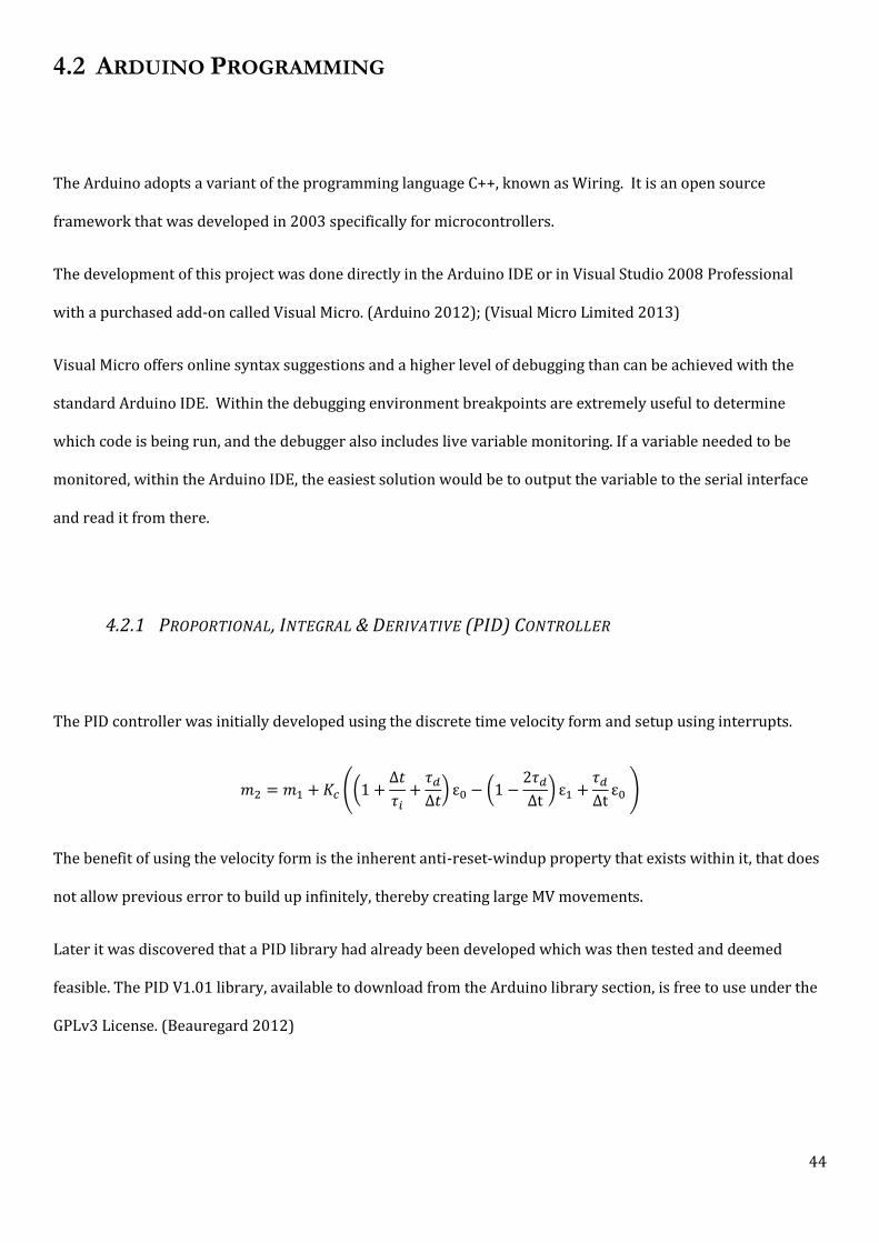
Figure 45 – Captured data of a non-aggressive PID tune with sample time of 20ms.
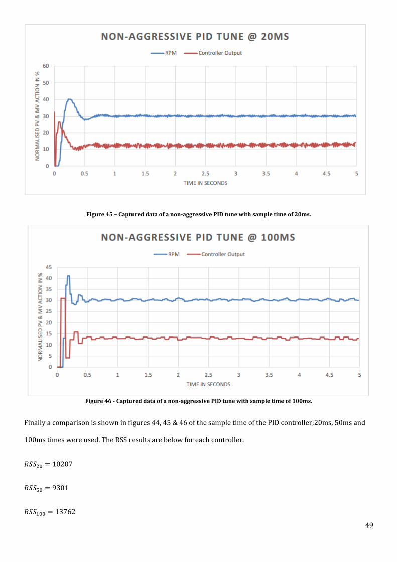
Figure 46 - Captured data of a non-aggressive PID tune with sample time of 100ms.
Finally a comparison is shown in figures 44, 45 & 46 of the sample time of the PID controller;20ms, 50ms and
100ms times were used. The RSS results are below for each controller.
𝑅𝑆𝑆20 = 10207
𝑅𝑆𝑆50 = 9301
𝑅𝑆𝑆100 = 13762
50
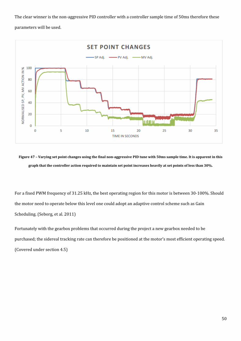
The clear winner is the non-aggressive PID controller with a controller sample time of 50ms therefore these
parameters will be used.
Figure 47 – Varying set point changes using the final non-aggressive PID tune with 50ms sample time. It is apparent in this
graph that the controller action required to maintain set point increases heavily at set points of less than 30%.
For a fixed PWM frequency of 31.25 kHz, the best operating region for this motor is between 30-100%. Should
the motor need to operate below this level one could adopt an adaptive control scheme such as Gain
Scheduling. (Seborg, et al. 2011)
Fortunately with the gearbox problems that occurred during the project a new gearbox needed to be
purchased; the sidereal tracking rate can therefore be positioned at the motor’s most efficient operating speed.
(Covered under section 4.5)
51
4.3 ASCOM
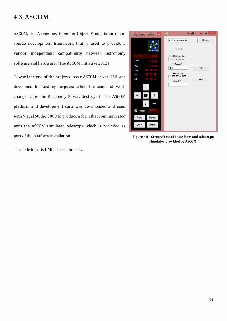
ASCOM, the Astronomy Common Object Model, is an open-
source development framework that is used to provide a
vendor independent compatibility between astronomy
software and hardware. (The ASCOM Initiative 2012)
Toward the end of the project a basic ASCOM driver HMI was
developed for testing purposes when the scope of work
changed after the Raspberry Pi was destroyed. The ASCOM
platform and development suite was downloaded and used
with Visual Studio 2008 to produce a form that communicated
with the ASCOM simulated telescope which is provided as
part of the platform installation.
The code for this HMI is in section 8.4.
Figure 48 – Screenshots of basic form and telescope
simulator provided by ASCOM.

52
5 CONCLUSION
This report has covered the ideas, design methodologies and tools used to achieve a substantial amount of
research and development for an automated telescope design. Unfortunately, throughout the project, the scope
for work has changed numerous times and mainly due to the mechanical failures or changes in specification.
Lacking expertise in mechanical systems the project soon lost traction and the scope reduced until only basic
sidereal tracking was conceivable.
The modification and development of 4-Byte floating point local sidereal time code was required due to the loss
of the Raspberry Pi at a late stage in the project and an efficient, robust PID controller design was used.
With the final failure of the aging gearbox the project became somewhat theoretical and little testing was able
to be achieved. However, with a new gearbox and basic machining the equipment will be ready to be used once
again for, at least, basic tracking.
Overall the project was an enormous learning curve and the final outcome will pave way for future
development and on that basis deemed somewhat successful.
53
6 FUTURE WORK RECOMMENDATIONS
6.1 GEARBOX DESIGN 4
As this project had many setbacks, a range of motors were purchased to be used as contingencies. When the
decision was made to use the original motor a number of extra gearboxes were ordered to cope with any
further setbacks given the issues experienced with manufacture of mounts and couplers.
TSINY Motor Industrial Co. Ltd. is a motor and gearbox manufacturer based in China, specialising in micro
motor and gearbox solutions with a wide range of products. After brief communication with a company
representative it was also discovered that they offer cost effective custom solutions.
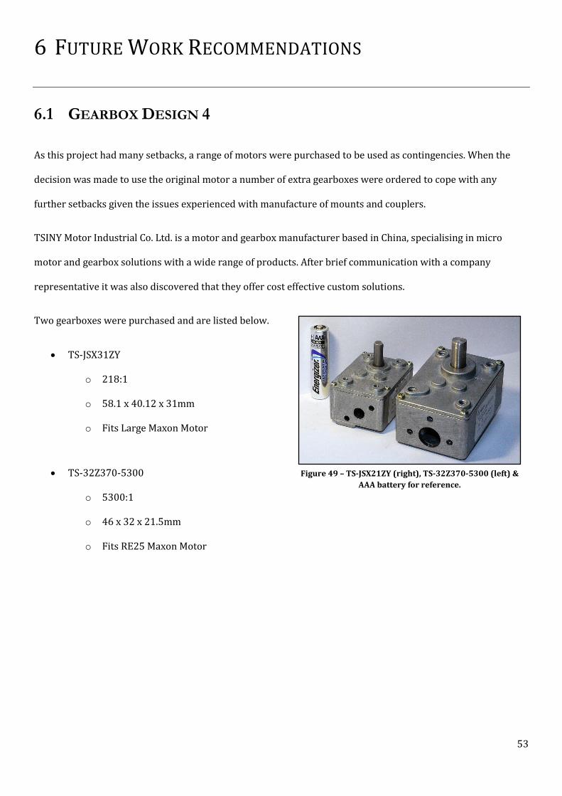
Two gearboxes were purchased and are listed below.
TS-JSX31ZY
o 218:1
o 58.1 x 40.12 x 31mm
o Fits Large Maxon Motor
TS-32Z370-5300
o 5300:1
o 46 x 32 x 21.5mm
o Fits RE25 Maxon Motor
Figure 49 – TS-JSX21ZY (right), TS-32Z370-5300 (left) &
AAA battery for reference.

54
6.2 ENVIRONMENT SENSORS
With the aim of the telescope to be mounted on the roof of the Murdoch Engineering building there will be a
requirement for some form of environmental monitoring. Seen in Figure 54 is a sensor that picks up rain drops
and a temperature & humidity sensor. The intention, when these were purchased, were to join the 𝐼2𝐶 bus and
be used to detect unsuitable conitions and put the system into lock-out mode where the telescope cannot be
activated remotely.
Figure 50 – Rain drop, temperature & humidity sensor to be used in future works. Battery used as size reference.

55
7 REFERENCES
3drenderblog. 2012. Raspberry Pi, Soft-emu vs Hard float [Updated]. 4 07. Accessed 08 01, 2013.
http://3drenderblog.wordpress.com/2012/07/04/raspberry-pi-soft-emu-vs-hard-float/.
Adafruit. 2013. Adding a Real Time Clock to Raspberry Pi. 27 02. Accessed 02 15, 2013.
http://learn.adafruit.com/adding-a-real-time-clock-to-raspberry-pi/set-rtc-time.
adama. 2012. memetic dot org. 13 07. Accessed 10 06, 2013. http://www.memetic.org/raspbian-
benchmarking-armel-vs-armhf/.
Arduino. 2013. Arduino Mega 2560. 08 05. Accessed 06 05, 2013.
http://arduino.cc/en/Main/ArduinoBoardMega2560.
—. 2012. Arduino Software. Accessed 07 29, 2012. http://arduino.cc/en/main/software.
Arduino.cc team. 2010. PWM_5steps. 26 10.
Avago Tech. 2013. HCTL-2032-SC. Accessed 9 1, 12.
http://www.avagotech.com/pages/en/motion_control_encoder_products/integrated_circuits/decoder_
ic/hctl-2032-sc/.
Beauregard, Brett. 2012. Arduino-PID-Library. 1 12. Accessed 01 15, 2013. https://github.com/br3ttb/Arduino-
PID-Library.
Berrangé, Daniel P. 2012. Entangle: Tethered Camera Control & Capture. Accessed 01 15, 2013. http://entangle-
photo.org.
Blavery. 2012. USB - The elephant in our room. 22 07. Accessed 05 25, 2013.
http://www.raspberrypi.org/phpBB3/viewtopic.php?t=12097.
Dingley, Andy. 2011. Arduino Mega2560. 14 07.
elinux.org. 2013. RPi Hardware. 4 3. Accessed 06 10, 2013. http://elinux.org/RPi_Hardware.
Freetronics. 2012. LEVEL: Logic Level Converter Module. Accessed 06 15, 2013.
http://www.freetronics.com/products/logic-level-converter-module#.Ub3Y4dzJOo4.
Ghassaei, Amanda. 2012. Arduino Timer Interrupts. 08 07. Accessed 09 01, 2013.
http://www.instructables.com/id/Arduino-Timer-Interrupts/.
Gittos. T., Mossop. B. 2013. “The Pilot Plant Case Study 2, 4 & 6.” Murdoch, WA.
Google Trends. 2013. Arduino, 8051, PICaxe, microchip. 22 08. Accessed 08 22, 2013.
http://www.google.com/trends/explore?q=arduino#q=arduino%2C%208051%2C%20PICaxe%2C%2
0microchip&cmpt=q.
Gremalm, Tim. 2013. Raspberry Pi PCB Overview Pinout v01. 27 05. Accessed 06 10, 2013.
http://upload.wikimedia.org/wikipedia/commons/9/97/Raspberrypi_pcb_overview_Pinout_v01.svg.
Grey, Dan. n.d. Sidreal Technology. Accessed 07 08, 2012. http://www.siderealtechnology.com/page2.html.
Jones, Ron H. 2009. Geared Drill Press. 26 03. Accessed 6 10, 2013.
https://en.wikipedia.org/wiki/File:Geared_drill_press.jpg.

56
Juneja, Pradeep K., A K. Ray, and R. Mitra. 2010. “Various Controller Design and Tuning Methods fro a First
Order Plus Dead Time Process.” International Journal of Computer Science & Communication 161-165.
Linfoot, E.H. 1956. “Colloquium on Schmidt optics.” The Observatory 170-177.
Machine Tool Help. 2010. Advantages & Disadvantages of Stepper motors & DC servo motors. Accessed 08 30,
2013. http://www.machinetoolhelp.com/Automation/systemdesign/stepper_dcservo.html.
maxim integrated. 2011. DS1307. 16 10. Accessed 01 15, 2013.
http://www.maximintegrated.com/datasheet/index.mvp/id/2688.
McKechnie, Glenn. 2006. Hwacheon Centre Lathe. 06. Accessed 06 10, 2013.
http://commons.wikimedia.org/wiki/File:HwacheonCentreLathe_460x1000.jpg.
MIT. 2000. “MIT 961.04 PWM.” Massachusetts Institute of Technology. 10.
http://fab.cba.mit.edu/classes/MIT/961.04/topics/pwm.pdf.
NASA Goddard Space Flight Centre. 1999. Solar Insolation. 06 07. Accessed 08 30, 2013.
http://education.gsfc.nasa.gov/experimental/July61999siteupdate/inv99Project.Site/Pages/solar.insol
ation.html.
NASA Learning Technologies Project. n.d. Telling Time by the Stars - Sidereal Time. Accessed 08 30, 2013.
http://www.grc.nasa.gov/WWW/k-
12/Numbers/Math/Mathematical_Thinking/telling_time_by_the_stars.htm.
Network Time Foundation. n.d. What is NTP? Accessed 08 15, 2013. http://www.ntp.org/ntpfaq/NTP-s-
def.htm.
New Mexico Tech. 2010. Sidereal.py: A Python package for astronomical calculations. 01 07. Accessed 09 01,
2013. http://infohost.nmt.edu/tcc/help/lang/python/examples/sidereal/.
Nguyen, Marie-Lan. 2007. Webcam Astrophotography . 15 09. Accessed 06 14, 2013.
http://commons.wikimedia.org/wiki/File:Webcam_astrophotography_2007_09_15.jpg.
Ogunnaike, Babatunde A., and W. Harmon Ray. 1994. Process Dynamics, Modeling and Control. New York: Oxford
University Press.
Pollock, Robert A. 2002. Meade SCTs. 1 1. http://www.telescopebluebook.com/sct/meade.htm.
Raspberry Pi Foundation. 2013. Raspberry Pi. Accessed 05 03, 2013. http://www.raspberrypi.org.
Raspbian. 2012. Raspbian. Accessed 05 02, 2013. http://www.raspbian.org/FrontPage.
Reinshaw. n.d. “Reinshaw.” RESOLUTE special solutions. Accessed 08 22, 2013.
http://www.renishaw.com/en/resolute-special-solutions--15694.
Robokits. n.d. Trex Dual Motor Controller DMC01. Accessed 08 30, 2013.
http://www.robokits.co.nz/trexmotorcontroller-777.
Seborg, Dale E., Duncan A. Mellichamp, Thomas F. Edgar, and Francis J. Doyle. 2011. Process Dynamics and
Control. Hoboken: John Wiley & Sons, Inc.
SparkFun Electronics. 2013. SparkFun. Accessed 1 10, 2013. https://www.sparkfun.com/.
Stanford University. n.d. “Electrical Engineering.” Stanford University.
http://www.stanford.edu/class/archive/ee/ee392m/ee392m.1056/Lecture14_MPC.pdf.

57
Starizona. 2013. CCD Imagine vs. Digital Camera Astrophotography. Accessed 06 14, 2013.
http://starizona.com/acb/ccd/introimagingccddigital.aspx.
Stepper World. 2001. Microstepping of Stepper Motors. Accessed 02 22, 2013.
http://www.stepperworld.com/Tutorials/pgMicrostepping.htm.
Sterrenkunde, Marty. 2004. Meade DeepSky Imager. 07 11. Accessed 06 10, 2013.
http://commons.wikimedia.org/wiki/File:Meade_DeepSky_Imager.jpg.
The ASCOM Initiative. 2012. Standards for Astronomy. Accessed 06 10, 2013. http://ascom-standards.org/.
The Engineering Toolbox. n.d. The Engineering Toolbox. Accessed 08 30, 2013.
http://www.engineeringtoolbox.com/ip-ingress-protection-d_452.html.
Torrone, Phillip. 2011. Make : Why the Arduino Won and Why It's Here to Stay. 10 02. Accessed 08 21, 2013.
http://makezine.com/2011/02/10/why-the-arduino-won-and-why-its-here-to-stay/.
trouch. 2013. Raspberry Pi benchmark. 12 01. Accessed 09 01, 2013.
http://trouch.com/2013/01/12/raspberry-pi-benchmark/.
Visual Micro Limited. 2013. visual micro ide. Accessed 08 30, 2013. http://www.visualmicro.com/.
Werther, J. 2007. Miniature Milling Machine. 2 10. Accessed 06 10, 2003.
http://commons.wikimedia.org/wiki/File:Miniature_milling_machine.jpg.
Wikimedia Commons. 2013. Rotary Encoder. 06 06. http://commons.wikimedia.org/wiki/File:Encoder_Disc_(3-
Bit).svg.

58
8 APPENDICES
8.1 RASPBERRY PI BUILD
8.1.1 OPERATING SYSTEM INSTALL
1. Download Raspbian ‘Wheezy’ from http://downloads.raspberrypi.org/ and extract it to a working
directory.
2. Download & install Win32 Disk Imager from http://sourceforge.net/projects/win32diskimager/ and
extract it to the working directory
3. Insert SD card into Windows based computer
4. Run Win32 Disk Imager as administrator
5. Choose SD card driver letter (i.e. E:\) and choose location of extracted image file (*.img)
6. Write to the card – process takes approx. 10 mins
7. Open Windows Explorer (Windows-Key + E) and browse to the drive letter. There should be less than
100MB in the root of the drive. The rest of the image is on an EXT3/4 linux based file system and won’t
be displayed in Windows without software.
8. Eject card and insert into Raspberry Pi
9. Power on Raspberry Pi with peripherals.

59
8.1.2 BASIC OS CONFIGURATION
1. The Raspberry Pi may not boot to terminal therefore you will need to plug it in the Ethernet connection
and have a DCHP server available to provide addressing. However if it does boot to terminal skip to step
4.
2. Determine the IP address via the DCHP server (router/application).
3. SSH to the Raspberry Pi using an application such as PuTTY
4. You will be prompted to configure the device by typing in ‘sudo raspi-config’
5. Change locale & time zone.
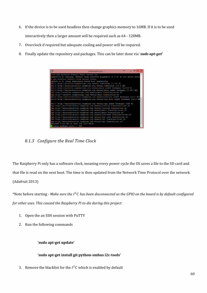
60
6. If the device is to be used headless then change graphics memory to 16MB. If it is to be used
interactively then a larger amount will be required such as 64 - 128MB.
7. Overclock if required but adequate cooling and power will be required.
8. Finally update the repository and packages. This can be later done via ‘sudo apt-get’
8.1.3 Configure the Real Time Clock
The Raspberry Pi only has a software clock, meaning every power cycle the OS saves a file to the SD card and
that file is read on the next boot. The time is then updated from the Network Time Protocol over the network.
(Adafruit 2013)
*Note before starting - Make sure the 𝐼2𝐶 has been disconnected as the GPIO on the board is by default configured
for other uses. This caused the Raspberry Pi to die during this project
1. Open the an SSH session with PuTTY
2. Run the following commands
‘sudo apt-get update’
‘sudo apt-get install git python-smbus i2c-tools’
3. Remove the blacklist for the 𝐼2𝐶 which is enabled by default
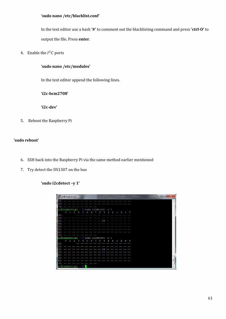
61
‘sudo nano /etc/blacklist.conf’
In the text editor use a hash ‘#’ to comment out the blacklisting command and press ‘ctrl-O’ to
output the file. Press enter.
4. Enable the 𝐼2𝐶 ports
‘sudo nano /etc/modules’
In the text editor append the following lines.
‘i2c-bcm2708’
‘i2c-dev’
5. Reboot the Raspberry Pi
‘sudo reboot’
6. SSH back into the Raspberry Pi via the same method earlier mentioned
7. Try detect the DS1307 on the bus
‘sudo i2cdetect –y 1’

62
8. Attempt to read the DS1307 over 𝐼2𝐶 using the following command
‘sudo hwclock-r’
Sat 1 Jan 2000 00:02:42 UTC -0.892464 seconds
*note if this doesn’t work check wiring is correct and make sure grounds from Raspberry
Pi and DS1307 are connected.
9. As this project planned on using Python to calculate Local Sidereal Time the following module is
required to have Python talk to the DS1307. From the shell type the following.
‘Mkdir GIT’
‘Cd GIT’
‘Git clone https://github.com/wyolum/Epoch.git’
‘Cd Epoch’
10. Test python can read the time
‘sudo python Epoch.py’
This should return a date and time stamp.
11. Forcing the Raspberry Pi to utilise the hardware clock instead of the software clock
‘sudo bash’
‘modprobe rtc-ds1307’
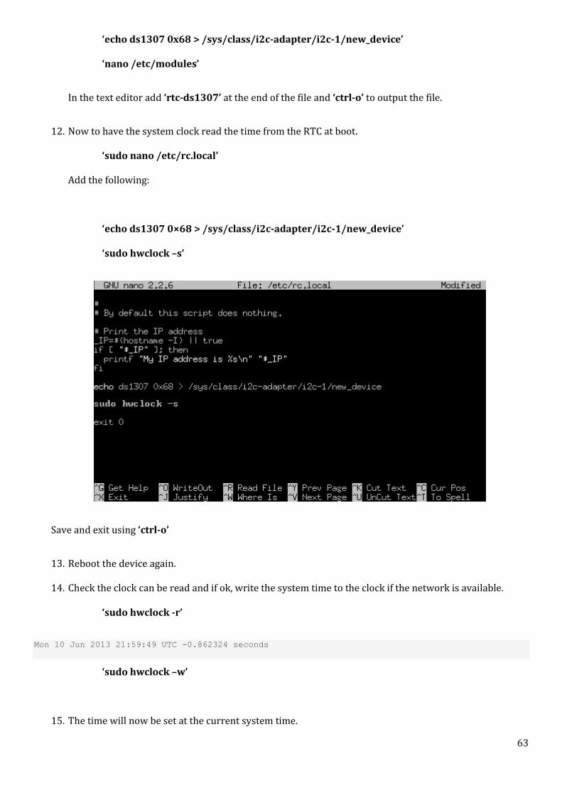
63
‘echo ds1307 0x68 > /sys/class/i2c-adapter/i2c-1/new_device’
‘nano /etc/modules’
In the text editor add ‘rtc-ds1307’ at the end of the file and ‘ctrl-o’ to output the file.
12. Now to have the system clock read the time from the RTC at boot.
‘sudo nano /etc/rc.local’
Add the following:
‘echo ds1307 0×68 > /sys/class/i2c-adapter/i2c-1/new_device’
‘sudo hwclock –s’
Save and exit using ‘ctrl-o’
13. Reboot the device again.
14. Check the clock can be read and if ok, write the system time to the clock if the network is available.
‘sudo hwclock -r’
Mon 10 Jun 2013 21:59:49 UTC -0.862324 seconds
‘sudo hwclock –w’
15. The time will now be set at the current system time.
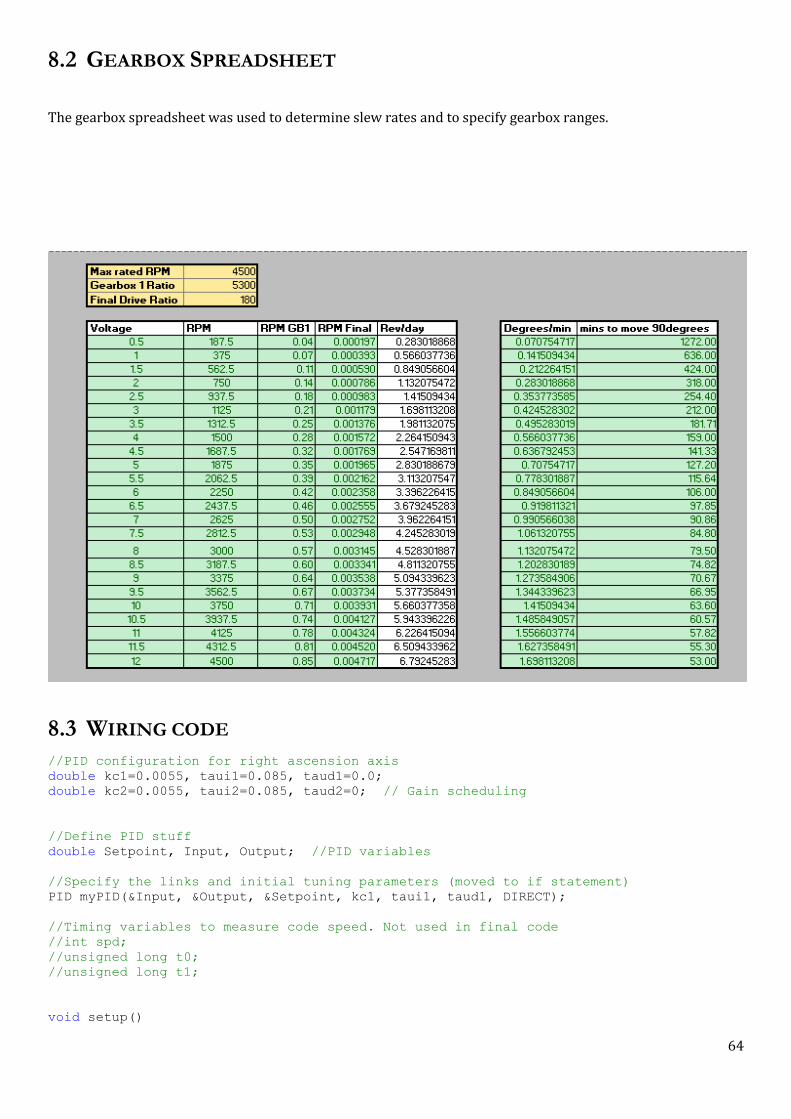
64
8.2 GEARBOX SPREADSHEET
The gearbox spreadsheet was used to determine slew rates and to specify gearbox ranges.
8.3 WIRING CODE
//PID configuration for right ascension axis
double kc1=0.0055, taui1=0.085, taud1=0.0;
double kc2=0.0055, taui2=0.085, taud2=0; // Gain scheduling
//Define PID stuff
double Setpoint, Input, Output; //PID variables
//Specify the links and initial tuning parameters (moved to if statement)
PID myPID(&Input, &Output, &Setpoint, kc1, taui1, taud1, DIRECT);
//Timing variables to measure code speed. Not used in final code
//int spd;
//unsigned long t0;
//unsigned long t1;
void setup()

65
{
Serial.begin(9600); //start serial bus at 9600bps
Serial.flush(); //flushes serial buffer
Wire.begin(); //setup arduino as master on i2c bus (no address)
//RTC startup
RTC.begin();
if (! RTC.isrunning()) {
Serial.println("RTC is NOT running!"); } // if the RTC can't be contacted print
error on serial
//RTC.adjust(DateTime(__DATE__, __TIME__)); // sets time from the prgramming
computer
//LCD startup
//lcd.init();
//lcd.backlight();
//Wire.onReceive(receiveEvent); // old code for receiving raspberry pi commands
//Motor channel port initilisation
//Channel A
pinMode(DirMotorRA, OUTPUT);
pinMode(BrkMotorRA, OUTPUT);
//Channel B
pinMode(DirMotorDec, OUTPUT);
pinMode(BrkMotorDec, OUTPUT);
//PID set sample time to 50ms
myPID.SetSampleTime(50) ;
// Initialize Timers
cli(); // disable global interrupts
// Counter Interupt
TCCR5A = 0; // set entire TCCR5A register to 0
TCCR5B = 0;
// set compare match register to desired timer count - using tables created choose a
value to match "real time" required.
OCR5A = 12499;
// turn on CTC (compare match or clear timer) mode:
TCCR5B |= (1 << WGM52);
// enable timer compare interrupt:
TIMSK5 |= (1 << OCIE5A);
// Set CS50 & CS51 bits so timer runs at 1/64th prescaler:
TCCR5B |= (1 << CS50);
TCCR5B |= (1 << CS51);
TCCR3B = TCCR3B & 0b11111000 | 0x01; //setup timer 3 to run at 31.5kHz
sei(); // enable global interrupts
}
//Sets real time clock based on the programming computers time. This will make the time
approx 10s delayed due to the upload time.
void RTCSet(){

66
RTC.adjust(DateTime(__DATE__, __TIME__)); // sets time from the prgramming
computer
}
// ******************************* MAIN LOOP ******************************\\
void loop()
{
String cmd ;
//ASCOM development
if(Serial.available()>0){
cmd = Serial.readStringUntil('#');
if (cmd=="GETLST"){
Serial.print(LST); Serial.println("#");
}
if (cmd=="GETElevation"){
Serial.print(Elevation); Serial.println("#");
}
if (cmd=="GETLat"){
Serial.print(Lattitude); Serial.println("#");
}
if (cmd=="RTCSet"){
RTCSet(); Serial.println("#");
}
}
myLSTfunction() ; //calls the LST calculation
//Forward
digitalWrite(DirMotorRA, HIGH);
digitalWrite(BrkMotorRA, LOW); //Disengage the Brake for Channel A
// PIDcontroller() ; //call PID function
//needto change this to have inputs of reverse or forward given the setpoint
//analogWrite(SpdMotorRA, analogRead(A4)/4);
// Just put in as a Soft switch for things during testing
//if (Serial.available() > 0)
// { incomingByte = Serial.read();
//
// return;}
//
//switch(incomingByte)
// {
// case '0':
//// Serial.println("FWD Motor 1");
//
//
// digitalWrite(BrkMotorRA, LOW);
// digitalWrite(DirMotorRA, HIGH);
//
//
// break;
//
// case '1':

67
//// Serial.println("REV Motor 1");
// digitalWrite(BrkMotorRA, HIGH);
// delay(200);
// digitalWrite(BrkMotorRA, LOW);
// digitalWrite(DirMotorRA, LOW);
//
// break;
//
// case '3':
//// Serial.println("Turn On Motor 1");
// startup() ;
// break;
// }
//Soft switch testing code finished
//
//
// Serial.print(" SP: ");
// Serial.print(analogRead(A4)*5.249);
Serial.print(" Input: ");
Serial.print(Input);
Serial.print(" Output: ");
Serial.println(Output);
Serial.print(" LST: ");
Serial.print(LST);
Serial.print(" Current JDN: ");
Serial.print(CurrentJDN);
Serial.print(" GMST ");
Serial.print(GMST);
Serial.print(" ");
Serial.print(now.year(), DEC);
Serial.print('/');
Serial.print(now.month(), DEC);
Serial.print('/');
Serial.print(now.day(), DEC);
Serial.print(' ');
Serial.print(now.hour(), DEC);
Serial.print(':');
Serial.print(now.minute(), DEC);
Serial.print(':');
Serial.print(now.second(), DEC);
Serial.println();
// Serial.print(" pidmode: ");
// Serial.print(pidmode);
// Serial.print(" MV1: ");
// Serial.print(100*Output/255);
// Serial.println("");
delay(10);
}
// *********************Interrupt Service Routines********************** \\
//50ms ISR for
ISR(TIMER5_COMPA_vect) {
Xcount = megaEncoderCounter.XAxisGetCount() ;
// constant of 0.6 is based on 1/dt *60s /2000CPR encoder
Input = (Xcount - Xlastcount)*0.6 ;

68
Xlastcount = Xcount; //sets lastcount to current count to be used next cycle in
speed calculations
PIDcontroller() ; //call PID function
//need to change this to have inputs of reverse or forward given the setpoint
}
// ***************************** Startup Routine ******************************\\
//Start-up procedure for the scope
//void startup()
// {
// while ( HomeSensor == LOW ) {
// digitalWrite(DirMotorRA,LOW);
// digitalWrite(BrkMotorRA, LOW);
//
// delay(50);
//
// analogWrite(SpdMotorRA,10) ; // reverse until the home sensor returns a high
pulse.
//
// megaEncoderCounter.XAxisReset(); //reset the encoder counter to this current
position.
//
// }
//
// ***************************** PID Routine ******************************\\
void PIDcontroller(){
//PID Controller Setpoint read - for testing
//Setpoint = analogRead(A4)*(motormax/1024); // 1024bit ADC reading POT into A4
Setpoint = 30;
myPID.SetMode(AUTOMATIC); //call PID library
//Gain scheduling of old maxon motor for better tracking at lower speeds.
if (Tracking == 1 ) //if tracking use non-aggressive PID values.
{ myPID.SetTunings(kc1, taui1, taud1); }
else
{ myPID.SetTunings(kc2, taui2, taud2); }
myPID.Compute() ; //compute the MV values
analogWrite(SpdMotorRA, Output); //write MV values
}
// *************************** LST Calculations ****************************\\
// http://www.mathworks.com.au/matlabcentral/fileexchange/28888-satellite-orbit-
computation/content/SGP4/siderealtime.m used to assist with coding
double myLSTfunction() {
DateTime now = RTC.now(); //calls RTC library to determine 'now' from clock
M = now.month();
Y = now.year();
D = now.day();
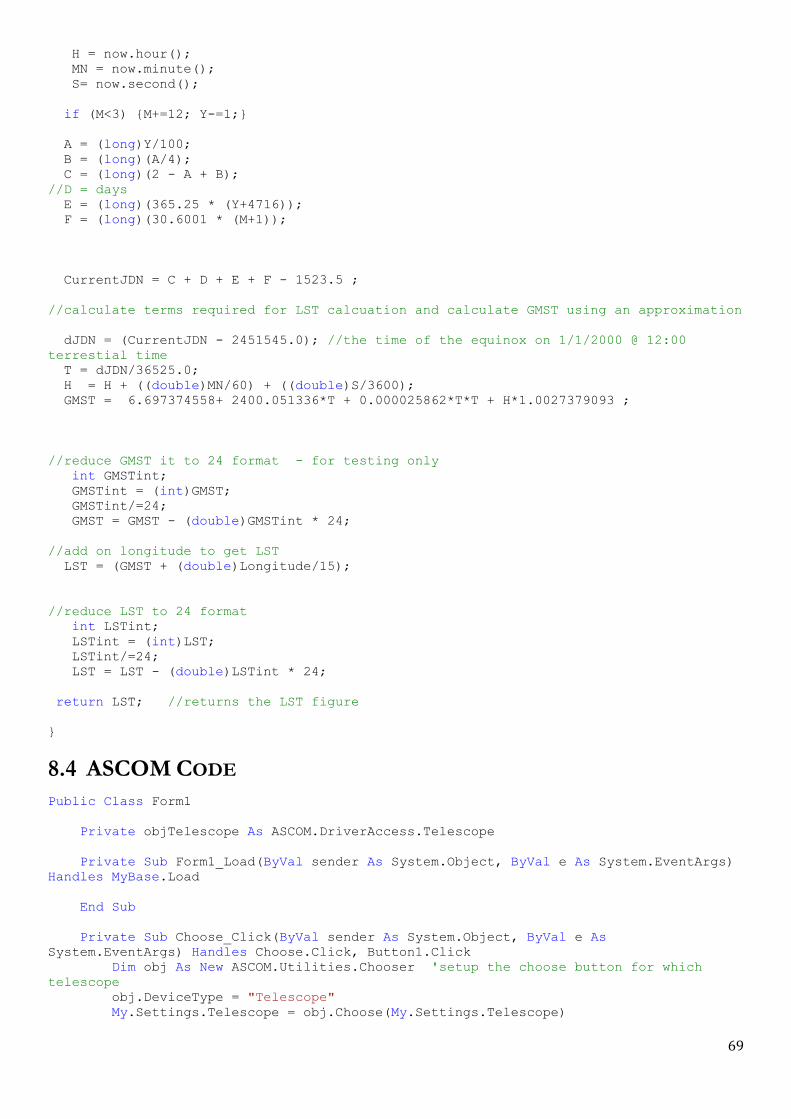
69
H = now.hour();
MN = now.minute();
S= now.second();
if (M<3) {M+=12; Y-=1;}
A = (long)Y/100;
B = (long)(A/4);
C = (long)(2 - A + B);
//D = days
E = (long)(365.25 * (Y+4716));
F = (long)(30.6001 * (M+1));
CurrentJDN = C + D + E + F - 1523.5 ;
//calculate terms required for LST calcuation and calculate GMST using an approximation
dJDN = (CurrentJDN - 2451545.0); //the time of the equinox on 1/1/2000 @ 12:00
terrestial time
T = dJDN/36525.0;
H = H + ((double)MN/60) + ((double)S/3600);
GMST = 6.697374558+ 2400.051336*T + 0.000025862*T*T + H*1.0027379093 ;
//reduce GMST it to 24 format - for testing only
int GMSTint;
GMSTint = (int)GMST;
GMSTint/=24;
GMST = GMST - (double)GMSTint * 24;
//add on longitude to get LST
LST = (GMST + (double)Longitude/15);
//reduce LST to 24 format
int LSTint;
LSTint = (int)LST;
LSTint/=24;
LST = LST - (double)LSTint * 24;
return LST; //returns the LST figure
}
8.4 ASCOM CODE
Public Class Form1
Private objTelescope As ASCOM.DriverAccess.Telescope
Private Sub Form1_Load(ByVal sender As System.Object, ByVal e As System.EventArgs)
Handles MyBase.Load
End Sub
Private Sub Choose_Click(ByVal sender As System.Object, ByVal e As
System.EventArgs) Handles Choose.Click, Button1.Click
Dim obj As New ASCOM.Utilities.Chooser 'setup the choose button for which
telescope
obj.DeviceType = "Telescope"
My.Settings.Telescope = obj.Choose(My.Settings.Telescope)

70
End Sub
Private Sub btnConnect_Click(ByVal sender As System.Object, ByVal e As
System.EventArgs) Handles btnConnect.Click
objTelescope = New ASCOM.DriverAccess.Telescope(My.Settings.Telescope)
objTelescope.Connected = True
sender.enabled = False
Timer1.Start() ' start the system timer to update text boxes
tbRA.Text = objTelescope.RightAscension
End Sub
Private Sub TextBox2_TextChanged(ByVal sender As System.Object, ByVal e As
System.EventArgs) Handles tbLST.TextChanged
End Sub
Private Sub Timer1_Tick(ByVal sender As System.Object, ByVal e As System.EventArgs)
Handles Timer1.Tick
tbLST.Text = objTelescope.SiderealTime 'update textboxes with data
tbPark.Text = objTelescope.AtPark
tbRA.Text = objTelescope.RightAscension
tbdRA.Text = objTelescope.RightAscensionRate
End Sub
Private Sub tbPark_TextChanged(ByVal sender As System.Object, ByVal e As
System.EventArgs) Handles tbPark.TextChanged
End Sub
Private Sub btnPark_Click(ByVal sender As System.Object, ByVal e As
System.EventArgs) Handles btnPark.Click
If objTelescope.AtPark Then
objTelescope.Unpark() 'unpark the scope
Else
objTelescope.Park() 'park the scope
End If
End Sub
Private Sub btnSlew_Click(ByVal sender As System.Object, ByVal e As
System.EventArgs) Handles btnSlew.Click
objTelescope.SlewToCoordinates(6.8, 87) 'test coordinates for slewing
End Sub
Private Sub Label2_Click(ByVal sender As System.Object, ByVal e As
System.EventArgs)
End Sub
End Class