Temperature elevation by HIFU in ex vivo porcine muscle:MRI measurement and simulation study

Maxim A. Solovchuka)

Center for Advanced Study in Theoretical Sciences (CASTS), National Taiwan University, Taipei 10617, Taiwan

San Chao Hwang and Hsu ChangMedical Engineering Research Division, National Health Research Institute, Miaoli 35053, Taiwan

Marc ThirietSorbonne Universités, UPMC Univ Paris 06, UMR 7598, Laboratoire Jacques-Louis Lions, F-75005,Paris, France

Tony W. H. Sheub)

Department of Engineering Science and Ocean Engineering, National Taiwan University, No. 1, Sec. 4,Roosevelt Road, Taipei 10617, Taiwan, Republic of China and Center for Advanced Study in TheoreticalSciences (CASTS), National Taiwan University, Taipei 10617, Taiwan

(Received 2 September 2013; revised 25 March 2014; accepted for publication 26 March 2014;published 18 April 2014)

Purpose: High-intensity focused ultrasound is a rapidly developing medical technology with a largenumber of potential clinical applications. Computational model can play a pivotal role in the planningand optimization of the treatment based on the patient’s image. Nonlinear propagation effects can sig-nificantly affect the temperature elevation and should be taken into account. In order to investigate theimportance of nonlinear propagation effects, nonlinear Westervelt equation was solved. Weak non-linear propagation effects were studied. The purpose of this study was to investigate the correlationbetween the predicted and measured temperature elevations and lesion in a porcine muscle.Methods: The investigated single-element transducer has a focal length of 12 cm, an aperture of8 cm, and frequency of 1.08 MHz. Porcine muscle was heated for 30 s by focused ultrasound trans-ducer with an acoustic power in the range of 24–56 W. The theoretical model consists of nonlinearWestervelt equation with relaxation effects being taken into account and Pennes bioheat equation.Results: Excellent agreement between the measured and simulated temperature rises was found. Forpeak temperatures above 85–90 ◦C “preboiling” or cavitation activity appears and lesion distortionstarts, causing small discrepancy between the measured and simulated temperature rises. From themeasurements and simulations, it was shown that distortion of the lesion was caused by the “preboil-ing” activity.Conclusions: The present study demonstrated that for peak temperatures below 85–90 ◦C numericalsimulation results are in excellent agreement with the experimental data in three dimensions. Bothtemperature rise and lesion size can be well predicted. Due to nonlinear effect the temperature in thefocal region can be increased compared with the linear case. The current magnetic resonance imaging(MRI) resolution is not sufficient. Due to the inevitable averaging the measured temperature can be10–30 ◦C lower than the peak temperature. Computational fluid dynamics can provide additionalimportant information that is lost using a state of the art MRI device. © 2014 American Associationof Physicists in Medicine. [http://dx.doi.org/10.1118/1.4870965]

Key words: HIFU, Westervelt equation, magnetic resonance guided high intensity focused ultrasound,porcine muscle

1. INTRODUCTION

High intensity focused ultrasound (HIFU) is a rapidly devel-oping medical technology for performing a noninvasive tumorablation surgery. This therapy has been successfully appliedto ablate solid malignant tumors in different organs such asprostate, breast, liver, pancreas, uterine fibroids.1–3 The ab-sorbed ultrasound energy in tissue is transformed into thethermal energy during focused therapy and this energy de-position can quickly elevate tissue temperature. Subject to thefocused ultrasound beam, thermal energy can be added pri-marily to a small region of tissues with little or no deposition

at all on the surrounding tissues. When tissue is heated to atemperature higher than 56 ◦C for 1 s, thermal coagulationnecrosis occurs.4 However, usually higher temperatures areused (65–85 ◦C) to ensure complete ablation of cancer cells.5

At an even higher temperature above 100 ◦C, tissue may boil,thereby leading to an unpredictable lesion growth4, 6, 7 andcausing necrosis of healthy tissues.

HIFU therapy is usually performed with magnetic res-onance imaging (MRI) or diagnostic US guidance. Thesetwo imaging procedures have their own advantages anddisadvantages.1 MRI is the only imaging modality thatcan measure tissue temperature elevation during focused

052903-1 Med. Phys. 41 (5), May 2014 © 2014 Am. Assoc. Phys. Med. 052903-10094-2405/2014/41(5)/052903/13/$30.00

052903-2 Solovchuk et al.: MRI temperature measurement and simulation study 052903-2

ultrasound treatment. The resulting temperature response canhelp to choose proper acoustic parameters during the treat-ment and reduce time needed for the treatment planning.However, MRI guidance is expensive and has limitations inspatial and temporal resolutions.1, 8, 9 MRI measures spatialand temporal average temperatures, and this can lead to an un-derestimation of the temperature.1, 8, 9 For example, in Ref. 8the numerical simulation results predicted the peak tempera-ture 100 ◦C after 7 s heating. Spatial averaging over the voxelvolume results in the temperature 73 ◦C, which agrees wellwith the measured MRI temperature. The temperatures mea-sured by MRI were underestimated by about 30% due to spa-tial averaging, which can lead to the errors in the estima-tion of the thermal dose (TD). US guidance can define tumorlocation, but it does not give information about tissue tem-perature and transient lesion monitoring is complicated. Thenecrosed volume is not very well visible by US imaging sothat lesion boundaries cannot be well localized. Gas bubblesare formed in the focal area and this region can be seen asan echogenic region. Treatment planning10–13 becomes there-fore very important for US imaging. Before the treatmentacoustic parameters of the transducer should be well adjustedin the case of US guided focused ultrasound therapy. Toavoid undesirable damage of healthy tissues, ultrasound beamshould be properly focused with a correct amount and pre-cise distribution of the deposited energy.14 Use of insufficientacoustic power may require repeated treatments or even dis-ease progression.15–17 For both imaging procedures treatmentplanning plays an important role. For MRI guided focused ul-trasound treatment planning is very important, when nonther-mal mechanisms15 are used in the treatment and temperaturemonitoring cannot be used as a guidance. A correct choice ofmathematical and physical models becomes therefore one ofthe crucial factors in the planning of therapeutic procedure.

Previously thermocouples were mostly used for the moni-toring of temperature and validation of the numerical model.18

Thermocouple can invasively measure the temperature at justone point. There are several drawbacks associated with theuse of thermocouples. First of all, it is difficult to control theposition of the thermocouple relative to the ultrasonic beam.Second, the presence of thermocouple can increase the heat-ing rate.19, 20 MRI permits the measurement of two- or three-dimensional temperature distribution that can be used to val-idate the model and does not have the drawbacks mentionedabove. In the present work, MRI temperature measurementshave been performed and compared with the numerical simu-lation results.

At high intensities nonlinear wave propagation effects leadto the distortion of waveform. Because of the nonlinear dis-tortion higher harmonics are generated. These higher harmon-ics are more readily absorbed by the tissue and can, in turn,improve the local heating. The two most popular nonlinearmodels chosen for the simulation of focused ultrasound fieldsare Khokhlov-Zabolotskaya-Kuznetsov (KZK) and Wester-velt equations. KZK equation is valid for directional soundbeams and can be applied to transducers with the aperture an-gles smaller than 16◦–18◦.21, 22 For wide aperture angles, it isbetter to use the more general Westervelt equation. The trans-

ducer in the current study has the aperture angle 19.4◦. Thenonlinear Westervelt equation is therefore chosen for the sim-ulation carried out in this paper.

Nonlinear propagation effects lead to the enhancedheating.7 When boiling appears lesion starts to grow towardthe transducer.6 In the current work, we are going to investi-gate the temperature elevation in a porcine muscle. Both MRImeasurement and numerical simulation have been performed.To the best of authors’ knowledge, it is the first time whenthree-dimensional temperature distribution measured by MRIhas been compared with the simulation results.

2. MATHEMATICAL MODEL

2.A. Nonlinear acoustic equation

Acoustic field generated by a HIFU source was modeledusing the nonlinear Westervelt equation23–25

∇2p − 1

c20

∂2p

∂t2+

[δ

c40

+ 2

c30

∑ν

cντν

1 + τν∂∂t

]∂3p

∂t3

+ β

ρ0c40

∂2p2

∂t2= 0. (1)

In the above, p is the sound pressure, β = 1 + B2A

is thecoefficient of nonlinearity, δ is the diffusivity of sound result-ing from fluid viscosity and heat conduction, τ ν is the relax-ation time, and cν is the small signal sound speed incrementfor the νth relaxation process. The first two terms describethe linear lossless wave propagating at a small-signal soundspeed. The third term denotes the loss due to thermal conduc-tion and fluid viscosity, and the fourth term accounts for therelaxation processes. The last term denotes acoustic nonlin-earity which may considerably affect thermal and mechanicalchanges within the tissue. Equation (1) can be transformed tothe coupled system of two partial differential equations givenbelow23

∇2p − 1

c20

∂2p

∂t2+ δ

c40

∂3p

∂t3+ β

ρ0c40

∂2p2

∂t2+

∑ν

Pν = 0,

(1 + τν

∂

∂t

)Pν = 2

c30

cντν

∂3p

∂t3. (2)

In the present paper, two relaxation processes (ν = 2) wereconsidered. Unknown relaxation parameters were calculatedby minimizing a mean square error between the linear attenu-ation law and relaxation model.23

For the linear Westervelt equation, the intensity is equal toIL = p2/2ρc0. For the nonlinear case, the total intensity is

I =∞∑

n=1

In, (3)

where In are the corresponding intensities for the respectiveharmonics nf0. The ultrasound power deposition per unit vol-ume is calculated as follows:

q =∞∑

n=1

2α(nf0)In. (4)

Medical Physics, Vol. 41, No. 5, May 2014

052903-3 Solovchuk et al.: MRI temperature measurement and simulation study 052903-3

The absorption in tissue shown above obeys the following fre-quency law:

α = α0

(f

f0

)η

, (5)

where α0 = 4.5 Np/m, η = 1.0, and f0 = 1 MHz.27

2.B. Energy equation for tissue heating

In a region free of large blood vessels, the diffusion-typePennes bioheat equation30 given below will be employed tomodel the transfer of heat in a perfused tissue region

ρt ct

∂T

∂t= kt∇2T − wb cb (T − T∞) + q. (6)

In the above energy equation proposed for modeling the time-varying temperature in the tissue domain, ρ, c, k denote thedensity, specific heat, and thermal conductivity, respectively,with the subscripts t and b referring to the tissue and blooddomains. The notation T∞ is denoted as the temperature at aremote location. In the present study, ex vivo porcine muscle isconsidered and the perfusion rate wb for the tissue cooling incapillary flow is equal to zero. The above energy equation forT is coupled with the Westervelt equation (1) for the acousticpressure through a power deposition term q defined in Eq. (4).Initially, we consider that the temperature is equal to 20 ◦C.On the wall a constant temperature of 20 ◦C was prescribed.A detailed description of the solution procedures can be foundin our previous papers.17, 23

Thermal dose developed by Sapareto and Dewey31 willbe applied to give us a quantitative relationship between thetemperature and time for the tissue heating and the extent ofcell killing. In focused ultrasound surgery (generally above50 ◦C), the expression for the TD can be written as

T D =∫ tfinal

t0

R(T −43)dt ≈tfinal∑t0

R(T −43)t, (7)

where R = 2 for T � 43 ◦C, R = 4 for 37 ◦C < T < 43 ◦C. Thevalue of TD required for a total necrosis ranges from 25 to240 min in biological tissues.31, 32 According to this relation,thermal dose resulting from heating the tissue to 43 ◦Cfor 240 min is equivalent to that achieved by heating thesame tissue to 56 ◦C for 1 s. In the current work, the value ofthermal dose equal to 240 min is considered for the predictionof the lesion shape.

3. THREE-POINT SIXTH-ORDER ACCURATESCHEME FOR WESTERVELT EQUATION

Discretization of the Westervelt equation (1) is started withthe approximation of temporal derivatives.23 Temporal deriva-tives were approximated by second-order accurate schemes as

follows:

∂2p

∂t2

∣∣∣∣n+1

= 2pn+1 − 5pn + 4pn−1 − pn−2

(t)2, (8)

∂3p

∂t3

∣∣∣∣n+1

= 6pn+1−23pn+34pn−1−24pn−2+8pn−3−pn−4

2(t)3.

(9)

The nonlinear term ∂2p2

∂t2 |n+1 is linearized using thesecond-order accurate relation

∂2p2

∂t2

∣∣∣∣n+1

= ∂

∂t

(∂p2

∂t

)=2

∂

∂t

(pn ∂p

∂t

∣∣∣∣n+1

+pn+1 ∂p

∂t

∣∣∣∣n

−pn ∂p

∂t

∣∣∣∣n)

= 2(2pn

t pn+1t + pnpn+1

t t + pn+1pntt − (

pnt

)2 − pnpntt

).

(10)

The above two approximation equations are then substitutedinto Eq. (1) to yield the following inhomogeneous Helmholtzequation:

uxx − ku = f (x). (11)

Development of a high-order scheme for Helmholtz equa-tion can be constructed by introducing more finite-differencestencil points. The improved prediction accuracy will be,however, at the cost of conducting matrix calculation. To re-tain the prediction accuracy without an expensive computa-tional cost, we are motivated to develop a scheme that cangive us the accuracy order of sixth in a grid stencil involvingonly three points. To achieve the above goal, the values of u(2),u(4), and u(6) are defined first at a nodal point j as follows:

u(2)|j = sj , u(4)|j = tj , u(6)|j = wj . (12)

The proposed compact difference scheme at xj relates t, s, andw with u as follows:

h6δ0wj +h4γ0tj +h2β0sj =α1uj+1+α0uj + α−1uj−1.

(13)

Substituting the Taylor-series expansion into Eq. (13) andconducting then a term-by-term comparison of the deriva-tives, the introduced free parameters are determined as α1

= α−1 = −1, α0 = 2, β0 = −1, γ0 = − 112 , and δ0 = − 1

360 .Since sj = kjuj + fj, the following two expressions for

tj = (k2j uj + 2kx,jux,j + kxx,j uj + kjfj + fxx,j ) and wj

= (k3j uj + 7kjujkxx,j + 6kjux,j kx,j + 4k2

x,j uj + 6kxx,j fj

+ 4kxxx,j ux,j +kxxxx,j uj + 4kx,j fx,j +kjfxx,j +fxxxx,j ) areresulted. Equation (13) can then be rewritten as

α1uj+1 + α1uj−1

+[α0 − β0 h2 kj − γ0 h4

(k2j + kxx,j

) − δ0 h6(k3j + 7kj kxx,j + +4k2

x,j + kxxxx,j

)]uj

= h2β0fj + h4γ0(2kx,jux,j + kjfj + fxx,j

) + h6δ0(k2fj + kfxx,j + fxxxx,j )

+h6δ0(6kjux,j kx,j + 6kxx,j fj + 4kxxx,j ux,j + 4kx,j fx,j ). (14)

Medical Physics, Vol. 41, No. 5, May 2014

052903-4 Solovchuk et al.: MRI temperature measurement and simulation study 052903-4

It follows that[1 −

(1

2h− kj+1h

12

) (1

360h6(4kxxx,j + 6kj kx,j ) + 1

6h4kx,j

)]uj+1

−[

2 + h2kj + 1

12h4

(k2j + kxx,j

) + 1

360h6

(k3j + 4k2

x,j + 7kj kxx,j + kxxxx,j

)]uj

+[

1 +(

1

2 h− kj−1 h

12

) (1

360h6(4 kxxx,j + 6 kj kx,j ) + h4 kx,j

6

)]uj−1

=[h2 + kjh

4

12+ 1

360h6

(k2j + 6kxx,j

)]fj + 1

90h6kx,j fx,j +

(1

360h6 kj + 1

12h4

)fxx,j

+ 1

360h6fxxxx,j +

[1

6h4kx,j + 1

360h6

(6kj kx,j + 4kxxx,j

)] ·[− h

12

(fj+1 − fj−1

)]. (15)

The corresponding modified equation for Eq. (11) using thecurrently proposed compact difference scheme can be derivedas follows after performing some algebraic manipulation:

uxx − ku = f +(

h6

20160

)u(8) +

(h8

1814400

)u(10)

+ . . . + HOT, (16)

where HOT denotes higher order terms. The above modifiedequation analysis sheds light that the Helmholtz scheme de-veloped within the three-point stencil framework can yield aspatial accuracy of sixth order.

Axisymmetric sound beam was considered. The Wester-velt equation was solved in cylindrical coordinates in con-junction with the alternating direction implicit solution algo-rithm. Nonreflecting radiation boundary condition was usedin the simulation. A sinusoidal waveform was considered tobe uniformly distributed over the transducer surface. Accu-racy of the numerical solutions has been examined23 by com-paring them with the known analytical and numerical solu-tions of other authors.33, 34

4. EXPERIMENTAL METHODS

A home-made MR-guided HIFU system, including HIFUtransducer, motion control system, and image processingsoftware, was constructed from basic elements in medicalengineering research division of National Health ResearchInstitute.35 A fixed focus spherical HIFU-transducer (focallength = 12 cm, operating frequency = 1.08 MHz, elec-troacoustic efficiency = 27.5%) was mounted on a waterbag placed above the object to be ablated. The ultrasoundpower attenuation through the water bag to the ablated ob-ject was less than 1.5%.35 The transducer was mounted ona nonmagnetic device to enable its movement along threeaxes. The software was written in C and JAVA languages.Our system has all the necessary functions to perform MR-guided HIFU ablation such as the HIFU power control, HIFUtransducer positioning, PC to MRI scanner communication,target temperature measurement, and ablated tissue necrosismonitoring.

Temperature measurement was based on the temperature-dependent proton resonance frequency (PRF) shift, whichworked well as the targets were abundant of water such asmuscle, liver, kindly, etc. The frequency shift can be derivedpixel-by-pixel from the phase difference between a referenceMRI image (unheated) and a measured MRI image (heated).Thank to our software, the MRI k-space data can be obtainedfrom MRI console to personal computer immediately afterthe completion of scanning. Afterwards, it was reconstructedto the magnitude image and the phase image. The magni-tude image was the ordinary MRI image, which showed theMRI anatomic contrast information, and the phase image wasused to calculate the temperature map. The magnitude imageand temperature map were fused with gray level and pseudocolor, respectively, to identify the hot spot of the ablated tis-sue. The MRI scanning and the temperature map display wereperformed continuously during the whole process of focusedultrasound ablation.

In the current study, two MRI scanning sequences, SPoiledGRadient echo (SPGR), and Inversion Recovery Turbo SpinEcho (IR-TSE) were used for different purposes. SPGR wasused to get the MRI temperature map such that it was set asfast as possible to get higher temporal resolution for a realtime HIFU ablation study. The drawback is that the signal-to-noise ratio (SNR) is lower and the spatial resolution is limited.To improve the signal-to-noise ratio, we set a thick slice thick-ness (8 mm) and low imaging resolution (2 mm per pixel)for the SPGR sequence. For the temperature measurementsalong the acoustic axis thinner slice thickness (3 mm) waschosen.

IR-TSE was used for denatured region identification af-ter HIFU ablation was finished. Higher spatial resolution wasused for this scanning sequence, the scanning time was there-fore longer. We set a thin slice thickness (6 mm), higher res-olution (1 mm per pixel), and repeated it twice to obtain theaverage value for the IR-TSE sequence.

Biological tissue is denatured by heat that changes its mag-netic resonance characteristic: longitudinal relaxation time(T1). The IR method was used to distinguish the denaturedregion from the surrounding area. By setting a specific valueof the inversion time (TI), the signal from either the denatured

Medical Physics, Vol. 41, No. 5, May 2014

052903-5 Solovchuk et al.: MRI temperature measurement and simulation study 052903-5

FIG. 1. Schematic of the experiment.

region or from the normal tissue can be eliminated.35 For ex-ample, in Fig. 7, while the inversion time was set as 550 ms,the image of normal porcine meat was almost suppressed andthe denatured region was enhanced.

A spoiled gradient echo sequence was chosen in a 1.5 TMRI scanner (Symphony, Siemens) with the following pa-rameters: TR = 13 ms, TE = 7 ms, flip angle = 30◦, datamatrix 128 × 128, field of view (FOV) = 256 × 256 mm,slice thickness = 8 mm. It took 1.7 s to get one MRI im-age. After HIFU ablation, the tissue necrosis evaluation wasperformed with IR-TSE (TR = 3000 ms, TE = 13 ms, TI= 550 ms, average = 2, matrix = 256 × 256, slice thickness= 6 mm).

The HIFU transducer used in this study is a single elementthat is spherically focused with an aperture of 8 cm and a fo-cal length of 12 cm. The experimental exposure was continu-ous for 30 s. In this study, the transducer with the frequencyf = 1.08 MHz was used. The efficiency of the home-madetransducer, which is equal to 27.5%, was measured by the ra-diation force balance method. Electric power of the transduceris varied from 80 to 200 W in our experiment. The measure-ments have been repeated for three times and the temperaturedifference was about 5%.

The schematic of the experiment is presented in Fig. 1. Thefocal point was located at location with the distance 3–3.5 cmbelow the surface of porcine muscle. We used as fresh as pos-sible a slice of pork. There was a water bag between the sliceof pork and the transducer.

5. RESULTS AND DISCUSSION

5.A. Pressure measurements

The transducer was calibrated in water in the followingsetting. The acoustic source and hydrophone were immersedin filtered and deionized water that is contained in a 74.5-cm-long, 36-cm-wide, and 50-cm-high tank, which is open tothe atmosphere. A three-dimensional computerized position-ing system is used to move the transducer along the beamaxis and orthogonal directions. The transducer was driven bya continuous wave.

In Fig. 2, the measured pressure profiles are plotted againstthe axial and radial distances (in the focal plane). The solidlines and open circles correspond to the prediction and mea-surement results, respectively. These results were obtained inwater at 25 ◦C using the chosen 0.4 mm hydrophone (OndaHNA-0400). The efficiency of the employed transducer wasmeasured using the radiation force balance method. The elec-tric energy of the transducer is equal to 1.9 W. The measuredacoustic pressures are normalized by the focal pressure of0.55 MPa. Good agreement between the measured and nu-merical results can be seen.

5.B. Tissue property measurements

Differences in acoustic and thermal properties of abdom-inal soft tissues may affect the delivery of thermal energy.Thermal lesions should be created accurately at the certainlocation without damaging the healthy tissues. The availabledata on tissue properties have some variations due to differ-ent measurement techniques and tissue types. Tissue proper-ties are patient specific and can also vary between tumors andhealthy tissues. In order to improve treatment planning, ac-curate characterization of the physical properties of tissue isrequired. During the treatment noninvasive methods of esti-mating thermal conductivity, perfusion and acoustic absorp-tion are necessary.28, 29 In the current work, ex vivo studywas considered, therefore the perfusion was equal to zero.

Axial distance, m

P

0.08 0.1 0.12 0.14 0.16 0.18

0.2

0.4

0.6

0.8

1

Radial distance, mm

P

0

0.2

0.4

0.6

0.8

1

5-5

FIG. 2. The measured (circles) and computed (solid line) pressure profiles in water at 1.08 MHz and 0.55 MPa pressure at the focal point.

Medical Physics, Vol. 41, No. 5, May 2014

052903-6 Solovchuk et al.: MRI temperature measurement and simulation study 052903-6

Time, t

Gau

ssia

nra

diu

ssq

uare

d,R

^2(t

)

0 5 10 15 200

5E-06

1E-05

1.5E-05

Experimental dataFitting line

FIG. 3. Measurement of thermal conductivity. Gaussian radius squared R2(t)is presented as function of time. The slope of the fitting line 5.74 × 10−7 isproportional to the thermal conductivity kt.

Noninvasive measurements of thermal diffusivity and acous-tic absorption have been performed.

The bioheat equation can be rewritten in the form

∂T

∂t= D∇2T + Q, (17)

TABLE I. Acoustic and thermal properties for the porcine muscle and water.

Tissue c0 ( ms ) ρ ( kg

m3 ) c ( Jkg K ) k ( W

m K ) α ( Npm ) β

Muscle 1550 1055 3200 0.49 4.5 4.5Water 1520 1000 4200 0.6 0.026 3.5

where the diffusivity D is equal to D = kt/ρtct and Q = q/

ρtct . Spatial distribution of focused ultrasound beam energydeposition can be approximated by three-dimensional Gaus-sian distribution. If we consider a very short heating, imme-diately after heating the temperature distribution can be fittedas a Gaussian function. This temperature distribution can beconsidered as an initial temperature. For the measurement ofthermal diffusivity, we will analyze the evolution of temper-ature during the cooling period. In Refs. 28 and 29, it wasshown that for a very short heating the solution of the bioheatequation T(r, z, t) at the focal plane z = zfocus can be writtenin the following form:

T (r, t) = A(t)exp( − r2

/(2σ 2

0xy + 4Dt))

= A(t)exp(−r2/R2(t)),

where σ 0xy is Gaussian variance in the radial plane at theend of the heating and R(t) is the Gaussian radius. The rate∂R2(t)/∂t, at which the Gaussian radius expands, depends only

z, m

P,M

Pa

0.09 0.1 0.11 0.12 0.13 0.14 0.15-6

-4

-2

0

2

4

6

P-

P+

z, m

q,W

/cm

^3

0.09 0.1 0.11 0.12 0.13 0.14 0.150

10

20

30

40

50

LinearNonlinear

z, m

T

0.1 0.11 0.12 0.13 0.14

40

60

80

100

120NonlinearLinear

r, mm

P,M

Pa

-5 0 5-6

-4

-2

0

2

4

6

P

P+

-

r, mm

q,W

/cm

^3

-5 0 50

10

20

30

40

50 LinearNonlinear

r, mm

T

-5 0 520

40

60

80

100

120LinearNonlinear

(a) (b) (c)

FIG. 4. The simulated linear (dashed-dotted) and nonlinear (solid) pressure (a), power deposition (b), and temperature (c) along the focal axis (upper row) andalong the radial axis in the focal plane (lower row) in a slice of pork for the case with electric power 200 W. Dashed-dotted vertical lines indicate the edges of avoxel.

Medical Physics, Vol. 41, No. 5, May 2014

052903-7 Solovchuk et al.: MRI temperature measurement and simulation study 052903-7

z

q, W

/cm

^3

0.06 0.08 0.1 0.12 0.14

40

LinearNonlinear

60

100

80

120

20

0

Z

T

0.1 0.11 0.12 0.13 0.14

40

60

80

100

NonlinearLinear

FIG. 5. The simulated linear (solid) and nonlinear (dashed-dotted) power deposition (left) and temperature (right) along the focal axis in the slice of pork forthe case with electric power 400 W.

on the thermal diffusivity

∂R2(t)

∂t= ∂

∂t

(2σ 2

0xy + 4Dt) = 4D = 4kt

ρtct

. (18)

To measure thermal conductivity, we will analyze the evo-lution of temperature spreading during the cooling period. Inour experiment, the tissue was heated for 2 s. Afterwards,the Gaussian radius was measured during the cooling pe-riod. In Fig. 3, the Gaussian radius squared is presented asfunction of time. The slope of the fitting line is m = 5.74× 10−7. The thermal conductivity is calculated as kt

= mρ tct/4 = 0.49 W/m ◦C.The assumptions used in this study for the measurements

of thermal conductivity are as follows: (1) tissue is consideredto be homogeneous; (2) heating was very fast; (3) tissue prop-erties (density, specific heat, thermal diffusivity) were consid-ered to be constant.

Speed of sound and attenuation coefficient weremeasured26 in porcine muscle prior to MRI temperaturemeasurements. The measured speed of sound is 1550 m/s,which agrees with the data of other authors.27 For themeasurement of absorption, we used the method proposed inRef. 36. Tissue properties used in the current simulation arelisted in Table I.27

5.C. Importance of acoustic nonlinearity effect

Figure 4 summarizes the results for linear and nonlinearsimulations carried out at different acoustic parameters andtemperatures in a slice of fresh pork. Acoustic pressure (a),power deposition (b), and temperature (c) are presented along

140 W 160 W 200 W

FIG. 6. Lesions (white area) formed in a slice of pork for different electricpowers: (a) 140, (b) 160, (c) 200 W. The transducer is located on the rightside of the investigated pork slice.

the focal axis (upper row) and along the radial axis (bottomrow) for the electric power 200 W. A full-width half pressuremaximum of the investigated transducer is 3 mm in the radialdirection and 3 cm along the focal axis for the linear acousticequation.

The peak positive and negative pressures are 5.6 and3.2 MPa, correspondingly. The peak negative pressure3.2 MPa lies below the cavitation threshold in a porkmuscle.37, 38 In Fig. 4(b), the peak power deposition has beenincreased by an amount of 16% from the linear to nonlinearwaveform. Nonlinear effects are found to be important onlyin a small region of the focal area. Nonlinear simulation re-sults shown in Fig. 4(c) indicate the peak temperature 115 ◦C,while the linear theory predicts only 109 ◦C. These simu-lated results show that nonlinear propagation effect can en-hance heating in the focal zone. In the present work, not veryhigh powers were considered, so the difference between the

FIG. 7. MRI image of lesions (in white) in porcine muscle for different elec-tric powers: 140, 160, 200 W.

Medical Physics, Vol. 41, No. 5, May 2014

052903-8 Solovchuk et al.: MRI temperature measurement and simulation study 052903-8

TABLE II. The predicted and measured lesion diameters and lesion lengthsat different electric powers.

Simulation Visual observation MRI imagePower (mm) in pork (mm) (mm)

140 W, length 23 24 21140 W, diameter 3 3 2160 W, length 28 31 25160 W, diameter 3.4 3 3

predicted linear and nonlinear temperature rises is about 7%.Although both linear and nonlinear theories predict temper-atures above 100 ◦C, nonlinear theory predicts “boiling” thatappears in a shorter time (18 s) in comparison with the lin-ear theory (22 s). When tissue temperature reaches 100 ◦C,vapor/gas bubbles, produced in the focal zone, can reflectand scatter the ultrasound beam, thereby complicating con-siderably the situation. The echogenic region in the focal areaappears and the lesion starts growing toward the transducer,thereby producing a tadpole shape.6, 7, 32 It was assumed thatbefore boiling the lesion grew almost symmetrically about thefocus and the lesion shape could be well predicted. Neglectingthe nonlinear effects in the treatment planning will lead to 4s underestimation of the “boiling” time. This underestimationcan lead to an undesirable damage of healthy tissues in frontof the focal region and insufficient ablation of tumor cells be-hind the focal region. For higher acoustic powers, the effectof acoustic nonlinearity will be larger. For 400 W of electricpower (112 W of acoustic power), the peak power depositionis increased by an amount of 45% from linear to nonlinearwaveform (Fig. 5). The difference between linear (89 ◦C) andnonlinear (103 ◦C) theories for the simulated peak tempera-tures will be 20%. Dashed-dotted vertical lines in Figs. 4(b)and 4(c) show the width of a voxel, which is 2 mm. The widthof a voxel is comparable with the full-width half pressuremaximum of the transducer (3 mm). Because MRI measuresvolume average temperature in a voxel, such a measured tem-perature will be lower than the peak temperature. In Figs. 4(b)

and 4(c), the boundaries of the voxel are presented for a casewhen the focal point is located at the center of the voxel.However, the focal point can be located anywhere in thevoxel. Depending on the focal point location the measuredtemperature can be quite different. For clinical doctors, theinformation about the difference between the measured andpeak temperatures is of high importance. We will thereforediscuss this important issue later in more details. Our empha-sis is to show how large the difference can be between themeasured and peak temperatures at different locations of thefocal point in the voxel.

5.D. MRI measurements and simulation results

In Fig. 6, the lesion shape is presented in a slice of freshpork under different electric powers. The transducer was lo-cated on the right side of the investigated pork slice. In Fig. 7,MRI lesion image is presented. For the case of 80 W, no le-sion was observed during the sonication. At the electric power140 W, the lesion has an ellipsoidal shape. In Table II, we cansee that the lesion predicted from the MRI image is smallerthan the real lesion in the pork slice due to the limitationsin the spatial resolution of MRI image. The lesion predictedfrom the MRI image is also smaller than the lesion predictedfrom simulation. There is a good agreement between the sim-ulated and measured lesion widths and lengths for 140 W. For160 W, only a small disagreement is seen between the simu-lated and measured lesion sizes. At 160 W, the lesion shape isslightly distorted from the ellipsoidal shape. A mild disagree-ment between the simulated and measured lesion lengths canbe seen. At 200 W, the lesion becomes different from the el-lipsoidal shape in the sense that lesion starts to grow towardthe transducer and has a “cone” shape. Peak negative pressureat 200 W is 3.2 MPa, which is below the cavitation thresholdin the pork muscle. Distortion of the lesion from an ellipsoidalshape cannot be explained any longer by the cavitation activ-ity. Growth of the lesion toward the transducer was attributedmainly to boiling.6, 7 At temperatures above 100 ◦C boiling

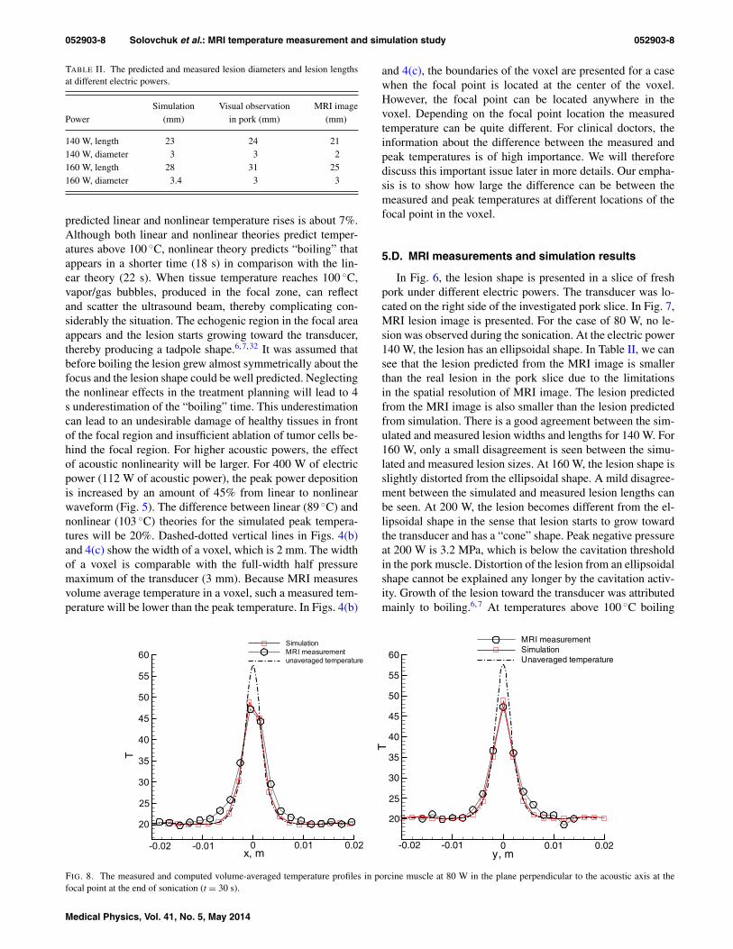
FIG. 8. The measured and computed volume-averaged temperature profiles in porcine muscle at 80 W in the plane perpendicular to the acoustic axis at thefocal point at the end of sonication (t = 30 s).

Medical Physics, Vol. 41, No. 5, May 2014

052903-9 Solovchuk et al.: MRI temperature measurement and simulation study 052903-9

x, m

T

0

40

50

60

70

80

90SimulationMRI measurementUnaveraged temperature

0.01-0.0120

30

y, m

T

0

30

40

50

60

70

80

90SimulationMRI measurementUnaveraged temperature

0.01-0.0120

FIG. 9. The measured and computed volume-averaged temperature profiles in porcine muscle at 140 W in the plane perpendicular to the acoustic axis at thefocal point at the end of sonication (t = 30 s).

in tissues appears. Prior to tissue boiling the lesion has beenfound to grow almost symmetrically about the focus and thelesion shape can be well predicted. Gas bubbles produced inthe focal zone can reflect and scatter ultrasound beam, therebycomplicating further the situation. The echogenic region inthe focal area appears and the lesion starts to grow toward thetransducer.

To compare the simulation and experimental results, it isnecessary to average the predicted temperature over the vol-ume of each voxel. The location of focal point inside the voxelis unknown. In the experiment, temperature distribution in theplane perpendicular to the acoustic axis at the focal point wasmeasured. We calculated the volume average temperaturesalong x and y axes. The calculated temperature profiles werethen compared with the experimental results. Afterwards, thelocation of the focal point inside the voxel was found. Fig-ures 8 and 9 plot the measured and computed volume averagetemperature profiles in porcine muscle at 80 and 140 W inthe plane perpendicular to the acoustic axis at the focal pointat the end of sonication (t = 30 s). An excellent agreementcan be observed between the predicted and simulated data

z, m

T

0.09 0.1 0.11 0.12 0.13 0.14 0.1520

40

60

80

SimulationMRI measurement

FIG. 10. The measured and computed volume-averaged temperature pro-files in porcine muscle at 140 W along the acoustic axis (t = 30 s).

along both x and y axes. In Fig. 10, a good agreement can alsobe observed between the predicted and simulated data alongthe acoustic axis z. There is a good agreement between thepredicted and simulated temperatures along all three axes. InFig. 11, the measured and computed volume average 2D tem-perature contours at 80 W are presented in the plane perpen-dicular to the acoustic axis at the focal point at the end ofsonication (t = 30 s). Good agreement can be seen betweenthe predicted and measured data.

In Fig. 12, the predicted temperature contours at t = 30 sare presented in the single voxel at the cross-section passingthrough the focal point for an electric power 140 W for differ-ent focal point locations inside the voxel. The predicted peaktemperature is 84 ◦C. Simulations show that depending on thelocation of the focal point in the voxel the measured peakspatial average temperature can be in the range from 60 ◦C[Fig. 12(b), focal point at the edge of the voxel] to 75 ◦C[Fig. 12(a), focal point in the center of voxel]. The real loca-tion of the focal point in Fig. 12(c) is shifted by y = 0.8 mmand x = 0.1 mm from the voxel center. The measured spa-tial average temperature in the voxel is 66 ◦C. Due to the in-dispensable averaging, the measured temperature is 9–24 ◦Clower than the peak temperature depending on where the focalpoint location is in the voxel. Doctors should keep this find-ing in mind during the treatment. In Ref. 8, the experimentalequipment was adjusted in such a way that focal point wasalways located at the center of the voxel and it was no need tofind the location of the focal point. The authors in Ref. 8 found27 ◦C difference between the predicted temperature (100 ◦C)and the temperature measured by MRI (73 ◦C). However, dur-ing the HIFU surgery with MRI guidance focal point can belocated arbitrarily inside the voxel and this can affect the dif-ference between the measured and predicted temperature. Forpeak temperatures up to 100 ◦C the measured temperature canbe 10–30 ◦C lower than the peak temperature. This differ-ence also depends on transducer parameters and the size ofMRI voxel. Decrease of the size of MRI voxel will decreasethe difference between the peak temperature and measuredtemperature.

Medical Physics, Vol. 41, No. 5, May 2014

052903-10 Solovchuk et al.: MRI temperature measurement and simulation study 052903-10

(a) (b)

x

y

-0.01 -0.005 0 0.005 0.01-0.01

-0.005

0

0.005

0.01 T

42363024

x

y

-0.01 -0.005 0 0.005 0.01-0.01

-0.005

0

0.005

0.01 T

42363024

FIG. 11. The measured (a) and simulated (b) volume-averaged temperature contours in porcine muscle at 80 W at the plane perpendicular to the acoustic axisat the focal point at the end of sonication (t = 30 s).

x, mm

y,m

m

-1 -0.5 0 0.5 1-1

-0.5

0

0.5

1 T

807570656055504540353025

x, mm

y,m

m

0 0.5 1 1.50

0.2

0.4

0.6

0.8

1

1.2

1.4

1.6

1.8

T

807570656055504540353025

x, mm

y,m

m

-1 -0.5 0 0.5

0

0.5

1

1.5

T

807570656055504540353025

(a) (b) (c)

FIG. 12. The simulated temperature contours at t = 30 s in a single voxel in the cross-section at the focal point for an electric power 140 W for different focalpoint locations inside the voxel. Cross (+) denotes the focal point. (a) Focal point is in the center of the voxel, the simulated spatial average temperature in thevoxel is TAV G = 75 ◦C. (b) Focal point is close to the edge of the voxel, the simulated spatial average temperature in the voxel is TAV G = 60 ◦C. (c) Real focalpoint location, TAV G = 66 ◦C.

t, s

Tem

per

atur

eris

e,K

0 50 100

30

35

40

45

50

55

60

SimulationMRI measurementUnaveraged temperature

20

25

t, s

T

0 50 10020

30

40

50

60

70

80

90

SimulationMRI measurementUnaveraged temperature

(a) (b)

FIG. 13. The measured and computed volume-averaged temperature profiles as function of time in porcine muscle at electric powers (a) 80 and (b) 140 W atthe focal point for a 30 s sonication.

Medical Physics, Vol. 41, No. 5, May 2014

052903-11 Solovchuk et al.: MRI temperature measurement and simulation study 052903-11

t,s

T

20 40 60 80 100 12020

30

40

50

60

70

SimulationMRI measurement

(a) (b)

t,s

T

0 50 10020

40

60

80

100

SimulationMRI measurement

FIG. 14. The measured and computed volume-averaged temperature profiles as function of time in porcine muscle at different electric powers (a) 160 and(b) 200 W at the focus for a 30 s sonication.

T

0 0.0120

30

40

50

60

70 SimulationMeasurement

-0.01y, m

T

020

30

40

SimulationMeasurement

50

60

70

0.01 0.02-0.01

FIG. 15. The measured and computed volume-averaged temperature profiles in porcine muscle at 160 W in the cross-section at the focal point, t = 12.5 s.

x, m

T

0

SimulationMRI measure entm

0.01-0.0120

30

40

50

60

y, m

T

0 0.0220

30

40

50

60SimulationMRI measurement

0.01-0.01

FIG. 16. The measured and computed volume-averaged temperature profiles in porcine muscle at 200 W in the cross-section at the focal point, t = 10 s.

Medical Physics, Vol. 41, No. 5, May 2014

052903-12 Solovchuk et al.: MRI temperature measurement and simulation study 052903-12

y

z

-0.01 0 0.01-0.03

-0.02

-0.01

0

0.01

0.02

T

5048464442403836343230282624

y

z

-0.01 0 0.01-0.03

-0.02

-0.01

0

0.01

0.02

T

5048464442403836343230282624

FIG. 17. The measured (left) and computed (right) volume-averaged tem-perature profiles in porcine muscle at 160 W at the plane parallel to the acous-tic axis, t = 10 s.

In Fig. 13, we present the measured and computed volumeaverage temperature profiles at electric powers 80 and 140 Was functions of time in porcine muscle at focus. We can see theexcellent agreement between the experimental and simulationdata for both powers.

In Fig. 14, the measured and computed volume averagetemperature profiles for electric powers 160 and 200 W arepresented. For spatial average temperatures below 70 ◦C, oursimulated results plotted in Figs. 14–16 have excellent agree-ment with the experimental data. Our two-dimensional simu-lation results at the cutting plane along acoustic axis in Fig. 17are in a good agreement with the experimental data. For MRItemperatures above 70 ◦C, only a small discrepancy can beseen. The measured average temperature 70 ◦C correspondsto the peak temperature at the focal point in the range of 85–90 ◦C. For the electric power 160 W at the end of the soni-cation (t = 30 s), the predicted and measured peak tempera-tures are about 90 ◦C. In Fig. 6, we can see that for electricpower 160 W the lesion is slightly distorted and there is asmall disagreement between the predicted and measured le-sion lengths. For a peak temperature above 85–90 ◦C “pre-boiling” or cavitation activity appears. Peak negative pressureat 200 W is 3 MPa, which is below the cavitation thresholdin the tissue.37 However, at such a high temperature there isa large vapor pressure. Therefore, we can conclude that at alarge peak negative pressure boiling will appear at a lowertemperature (we will call it “preboiling”). Previously, 100 ◦Ctemperature was considered as a threshold value for a lesion todistort. After the current study, we believe that at a time whenthe temperature reaches 85–90 ◦C lesion can start growing to-ward the transducer.

6. CONCLUSION

Temperature elevation in a slice of fresh pork was investi-gated both experimentally and theoretically. Spatial and tem-

poral resolutions of the MRI thermometry were designed to beclose to the resolution used in the clinical practice. It has beenshown that nonlinear propagation effect can enhance heatingand boiling. There is an excellent agreement between the mea-sured and simulated temperature rise. For peak temperaturesabove 85–90 ◦C, “preboiling” or cavitation activity appearsand lesion distortion starts and we get only a small discrep-ancy between the simulated and measured results. From themeasurements and simulations, it was shown that distortion ofthe lesion was caused by the preboiling event. Several math-ematical models39 are available for the analysis of temper-ature elevation and lesion evolution during thermal therapy.For the current mathematical model, excellent agreement be-tween the theory and experimental data for the temperaturerise and lesion size was found for all the studied power levelsfor peak temperatures below 85–90 ◦C. The current numeri-cal model is applicable to the case while the peak temperatureis below 85–90 ◦C. At higher temperatures, it is necessary totake into account the effects of boiling and cavitation. MRImeasures volume average temperature. Because of the indis-pensable averaging procedure, the measured temperature canbe 10–30 ◦C lower (depending on the focal point location in-side the voxel) than the peak temperature. The measured tem-perature 70–90 ◦C may, for example, correspond to the peaktemperature 100 ◦C. This finding should be taken into accountduring the treatment. The current MRI resolution is not suf-ficient and computational fluid dynamics is therefore a usefultool to provide additional important information that is lostusing a state of the art MRI device.

ACKNOWLEDGMENTS

The authors would like to acknowledge the financial sup-port from the Center for Advanced Study in Theoretical Sci-ences (CASTS) and from the National Science Council ofRepublic of China under Contract No. NSC102-2811-M-002-125. The authors also would like to thank Dr. I. Kuo from Na-tional Health Research Institutes, Taiwan, for his assistanceto set up pressure measurements and perform sound speedmeasurement.

a)Electronic mail: solovchuk@gmail.comb)Electronic mail: twhsheu@ntu.edu.tw1Y. F. Zhou, “High intensity focused ultrasound in clinical tumor ablation,”World J. Clin. Oncol. 2, 8–27 (2011).

2T. A. Leslie and J. E. Kennedy, “High intensity focused ultrasound in thetreatment of abdominal and gynaecological diseases,” Int. J. Hypertherm.23, 173–182 (2007).

3O. Al-Bataineha, J. Jenneb, and P. Huberb, “Clinical and future applicationsof high intensity focused ultrasound in cancer,” Cancer Treatment Rev. 38,346–353 (2012).

4N. T. Wright and J. D. Humphrey, “Denaturation of collagen via heating:An irreversible rate process,” Annu. Rev. Biomed. Eng. 4, 109–128 (2002).

5A. Napoli, M. Anzidei, F. Ciolina, E. Marotta, B. C. Marincola, G. Bra-chetti, L. D. Mare, G. Cartocci, F. Boni, V. Noce, L. Bertaccini, andC. Catalano, “MR-guided high-intensity focused ultrasound: Current sta-tus of an emerging technology,” Cardiovasc. Interv. Radiol. 36, 1190–1203(2013).

6W. S. Chen, C. Lafon, T. J. Matula, S. Vaezy, and L. A. Crum, “Mechanismsof lesion formation in high intensity focused ultrasound therapy,” Acoust.Res. Lett. Online 4, 41–46 (2003).

Medical Physics, Vol. 41, No. 5, May 2014

052903-13 Solovchuk et al.: MRI temperature measurement and simulation study 052903-13

7V. A. Khokhlova, M. R. Bailey, J. A. Reed, B. W. Cunitz, P. J. Kaczkowski,and L. A. Crum, “Effects of nonlinear propagation, cavitation and boilingin lesion formation by high intensity focused ultrasound in a gel phantom,”J. Acoust. Soc. Am. 119, 1834–1848 (2006).

8T. D. Khokhlova, M. S. Canney, D. Lee, K. I. Marro, L. A. Crum,V. A. Khokhlova, and M. R. Bailey, “Magnetic resonance imaging of boil-ing induced by high intensity focused ultrasound,” J. Acoust. Soc. Am. 125,2420–2431 (2009).

9S. D. Sokka, R. King, and K. Hynynen, “MRI-guided gas bubble enhancedultrasound heating in in vivo rabbit thigh,” Phys. Med. Biol. 48, 223–241(2003).

10M. A. Solovchuk, T. W. H. Sheu, and M. Thiriet, “Effects of acoustic non-linearity and blood flow cooling during HIFU treatment,” AIP Conf. Proc.1503, 83–88 (2012).

11M. A. Solovchuk, T. W. H. Sheu, and M. Thiriet, “Image-based computa-tional model for focused ultrasound ablation of liver tumor,” J. Comput.Surg. 1, 4 (13pp.) (2014).

12A. Pulkkinen and K. Hynynen, “Computational aspects in high intensityultrasonic surgery planning,” Comput. Med. Imaging Graph. 34, 69–78(2010).

13T. W. H. Sheu, M. A. Solovchuk, A. W. J. Chen, and M. Thiriet, “Onan acoustics-thermal-fluid coupling model for the prediction of tempera-ture elevation in liver tumor,” Int. J. Heat Mass Transfer 54, 4117–4126(2011).

14T. Yu and J. Luo, “Adverse events of extracorporeal ultrasound guided highintensity focused ultrasound therapy,” PLoS ONE 6, e26110 (2011).

15D. Schlesinger, S. Benedict, C. Duederich, A. Klibanov, and J. Larner,“MRI-guided focused ultrasound surgery, present and future,” Med. Phys.40, 080901 (32pp.) (2013).

16M. A. Solovchuk, T. W. H. Sheu, W. L. Lin, I. Kuo, and M. Thiriet, “Simu-lation study on acoustic streaming and convective cooling in blood vesselsduring a high-intensity focused ultrasound thermal ablation,” Int. J. HeatMass Transfer 55, 1261–1270 (2012).

17M. A. Solovchuk, T. W. H. Sheu, M. Thiriet, and W. L. Lin, “On a com-putational study for investigating acoustic streaming and heating duringfocused ultrasound ablation of liver tumor,” J. Appl. Therm. Eng. 56(1–2),62–76 (2013).

18S. Maruvada, Y. Liu, W. F. Pritchard, B. A. Herman, and G. R. Harris,“Comparative study of temperature measurements in ex vivo swine muscleand a tissue-mimicking material during high intensity focused ultrasoundexposures,” Phys. Med. Biol. 57(1), 1–19 (2012).

19J. Huang, R. G. Holt, R. O. Cleveland, and R. A. Roy, “Experimental vali-dation of a tractable medical model for focused ultrasound heating in flow-through tissue phantoms,” J. Acoust. Soc. Am. 116, 2451–2458 (2004).

20R. L. Clarke and G. R. ter Haar, “Temperature rise recorded during lesionformation by high-intensity focused ultrasound,” Ultrasound Med. Biol. 23,299–306 (1997).

21J. N. Tjotta, S. Tjotta, and E. H. Vefring, “Effects of focusing on the non-linear interaction between two collinear finite amplitude sound beams,” J.Acoust. Soc. Am. 89, 1017–1027 (1991).

22J. E. Soneson, “A parametric study of error in the parabolic approxima-tion of focused axisymmetric ultrasound beams,” J. Acoust. Soc. Am. 131,EL481–EL485 (2012).

23M. A. Solovchuk, T. W. H. Sheu, and M. Thiriet, “Simulation of nonlinearWestervelt equation for the investigation of acoustic streaming and nonlin-ear propagation effects,” J. Acoust. Soc. Am. 134(5), 3931–3942 (2013).

24M. F. Hamilton and C. L. Morfey, “Model equations,” in Nonlinear Acous-tics, edited by M. F. Hamilton and D. T. Blackstock (Academic, Boston,1998), Chap. 3.

25Y. Jing and R. O. Cleveland, “Modeling the propagation of nonlinear three-dimensional acoustics beams in inhomogeneous media,” J. Acoust. Soc.Am. 122, 1352–1364 (2007).

26I. Y. Kuo and K. K. Shung, “A novel method for the measurement of acous-tic speed,” J. Acoust. Soc. Am. 88, 1679–1682 (1990).

27F. A. Duck, Physical Property of Tissues - A Comprehensive ReferenceBook (Academic, London, 1990), p. 346.

28H. L. Cheng and D. B. Plewes, “Tissue thermal conductivity by magneticresonance thermometry and focused ultrasound heating,” J. Magn. Reson.Imaging 16(5), 598–609 (2002).

29J. Zhang, C. Mougenot, A. Partanen, R. Muthupillai, and P. H. Hor, “Vol-umetric MRI-guided high-intensity focused ultrasound for noninvasive, invivo determination of tissue thermal conductivity: Initial experience in apig model,” J. Magn. Reson. Imaging 37(4), 950–957 (2013).

30H. H. Pennes, “Analysis of tissue and arterial blood temperature in theresting human forearm,” J. Appl. Physiol. 1, 93–122 (1948).

31S. A. Sapareto and W. C. Dewey, “Thermal dose determination in cancertherapy,” Int. J. Radiat. Oncol., Biol., Phys. 10, 787–800 (1984).

32P. M. Meaney, M. D. Cahill, and G. R. ter Haar, “The intensity depen-dence of lesion position shift during focused ultrasound surgery,” Ultra-sound Med. Biol. 26, 441–450 (2000).

33D. T. Blackstock, “Connection between the Fay and Fubini solutions forplane sound waves of finite amplitude,” J. Acoust. Soc. Am. 39, 1019–1026(1966).

34H. T. O’Neil, “Theory of focusing radiators,” J. Acoust. Soc. Am. 21(5),516–526 (1949).

35S. C. Hwang, C. Yao, I. Y. Kuo, W. C. Tsai, and H. Chang, “Tissue necrosismonitoring for HIFU ablation with T1 contrast MRI imaging,” AIP Conf.Proc. 1359, 157–162 (2011).

36U. Vyas, A. Payne, N. Todd, D. L. Parker, R. B. Roemer, and D. A. Chris-tensen, “Non-invasive patient-specific acoustic property estimation forMR-guided focused ultrasound surgery,” AIP Conf. Proc. 1481, 419–425(2012).

37K. Hynynen, “The threshold for thermally significant cavitation in dog’sthigh muscle in vivo,” Ultrasound Med. Biol. 17, 157–169 (1991).

38T. Li, H. Chen, T. Khokhlova, Y. N. Wang, W. Kreider, X. He, andJ. H. Hwang, “Passive cavitation detection during pulsed HIFU exposuresof ex vivo tissues and in vivo mouse pancreatic tumors,” Ultrasound Med.Biol. (in press).

39S. J. Payne, T. Peng, and D. P. O’Neill, “Mathematical modeling of thermalablation,” Crit. Rev. Biomed. Eng. 38(1), 21–30 (2010).

Medical Physics, Vol. 41, No. 5, May 2014