Templates for Linear Algebra Problems

Zhaojun Bai

University of Kentucky

David Day

University of Kentucky

James Demmel

University of California - Berkeley

Jack Dongarra

University of Tennessee and Oak Ridge National Laboratory

Ming Gu

University of California - Berkeley

Axel Ruhe

Chalmers University of Technology, G�oteborg

and

Henk van der Vorst

Utrecht University

Abstract. The increasing availability of advanced-architecture computers is having a very

signi�cant e�ect on all spheres of scienti�c computation, including algorithm research andsoftware development in numerical linear algebra. Linear algebra {in particular, the solution

of linear systems of equations and eigenvalue problems { lies at the heart of most calculations in

scienti�c computing. This chapter discusses some of the recent developments in linear algebradesigned to help the user on advanced-architecture computers.

Much of the work in developing linear algebra software for advanced-architecture computers

is motivated by the need to solve large problems on the fastest computers available. In thischapter, we focus on four basic issues: (1) the motivation for the work; (2) the development

of standards for use in linear algebra and the building blocks for a library; (3) aspects of

templates for the solution of large sparse systems of linear algorithm; and (4) templates forthe solution of large sparse eigenvalue problems. This last project is under development and

we will pay more attention to it in this chapter.

1 Introduction and Motivation

Large scale problems of engineering and scienti�c computing often require solutions of linear algebra

problems, such as systems of linear equations, least squares problems, or eigenvalue problems. There

is a vast amount of material available on solving such problems, in books, in journal articles, and as

software. This software consists of well-maintained libraries available commercially or electronically

in the public-domain, other libraries distributed with texts or other books, individual subroutines

tested and published by organizations like the ACM, and yet more software available from individuals

or electronic sources like Netlib [21], which may be hard to �nd or come without support. So although

many challenging numerical linear algebra problems still await satisfactory solutions, many excellent

methods exist from a plethora of sources.

? This work was made possible in part by grants from the Defense Advanced Research Projects Agency under

contract DAAL03-91-C-0047 administered by the Army Research O�ce, the O�ce of Scienti�c ComputingU.S. Department of Energy under Contract DE-AC05-84OR21400, the National Science Foundation Sci-

ence and Technology Center Cooperative Agreement No. CCR-8809615, and National Science Foundation

Grant No. ASC-9005933.

But the sheer number of algorithms and their implementationsmakes it hard even for experts, let

alone general users, to �nd the best solution for a given problem. This has led to the development of

various on-line search facilities for numerical software. One has been developed by NIST (National

Institute of Standards and Technology), and is called GAMS (Guide to Available Mathematical

Software) [7]; another is part of Netlib [21]. These facilities permit search based on library names,

subroutines names, keywords, and a taxonomy of topics in numerical computing. But for the general

user in search of advice as to which algorithm or which subroutine to use for her particular problem,

they o�er relatively little advice.

Furthermore, many challenging problems cannot be solved with existing \black-box" software

packages in a reasonable time or space. This means that more special purpose methods must be

used, and tuned for the problem at hand. This tuning is the greatest challenge, since there are a large

number of tuning options available, and for many problems it is a challenge to get any acceptable

answer at all, or have con�dence in what is computed. The expertise regarding which options, or

combinations of options, is likely to work in a speci�c application area, is widely distributed.

Thus, there is a need for tools to help users pick the best algorithm and implementation for their

numerical problems, as well as expert advice on how to tune them. In fact, we see three potential

user communities for such tools:

{ The \HPCC" (High Performance Computing and Communication) community consists of those

scientists trying to solve the largest, hardest applications in their �elds. They desire high speed,

access to algorithmic details for performance tuning, and reliability for their problem.

{ Engineers and scientists generally desire easy-to-use, reliable software, that is also reasonably

e�cient.

{ Students and teachers want simple but generally e�ective algorithms, which are easy to explain

and understand.

It may seem di�cult to address the needs of such diverse communities with a single document.

Nevertheless, we believe this is possible in the form of templates.

A template for an algorithm includes

1. A high-level description of the algorithm.

2. A description of when it is e�ective, including conditions on the input, and estimates of the time,

space or other resources required. If there are natural competitors, they will be referenced.

3. A description of available re�nements and user-tunable parameters, as well as advice on when

to use them.

4. Pointers to complete or partial implementations, perhaps in several languages or for several

architectures (each parallel architecture). These implementation expose those details suitable

for user-tuning, and hide the others.

5. Numerical examples, on a common set of examples, illustrating both easy cases and di�cult

cases.

6. Trouble shooting advice.

7. Pointers to texts or journal articles for further information.

In addition to individual templates, there will be a decision tree to help steer the user to the right

algorithm, or subset of possible algorithms, based on a sequence of questions about the nature of

the problem to be solved.

Our goal in this paper is to outline such a set of templates for systems of linear equations and

eigenvalue problems. The main theme is to explain how to use iterative methods.

The rest of this paper is organized as follows. Section 2 discusses related work. Section 3 describes

the work we have done on templates for sparse linear systems. Section 4 described our taxonomy

of eigenvalue problems and algorithms, which we will use to organize the templates and design a

decision tree. Section 4.1 discusses notation and terminology. Sections 4.2 through 4.7 below describe

the decision tree in more detail. Section 4.8 outlines a chapter on accuracy issues, which is meant to

describe what accuracy one can expect to achieve, since eigenproblems can be very ill-conditioned,

as well as tools for measuring accuracy. Section 4.9 describes the formats in which we expect to

deliver both software and documentation.

This paper is a design document, and we encourage feedback, especially from potential users.

2 Related Work

Many excellent numerical linear algebra texts [43, 25, 30, 11, 33] and black-box software libraries

[36, 24, 1] already exist. A great deal of more specialized software for eigenproblems also exists, for

example, for surveys on the subject see [31, 4].

A book of templates, including software, has already been written for iterative methods for solving

linear systems [6], although it does not include all the ingredients mentioned above. In particular,

it discusses some important advanced methods, such as preconditioning, domain decomposition and

multigrid, relatively brie y, and does not have a comprehensive set of numerical examples to help

explain the expected performance from each algorithm on various problem classes. It has a relatively

simple decision tree to help users choose an algorithm.Nevertheless, it successfully incorporates many

of the features we wish to have.

The linear algebra chapter in Numerical Recipes [32] contains a brief description of the conjugate

gradient algorithm for sparse linear systems and the eigensystem chapter only contains the basic

method for solving dense standard eigenvalue problem, all of the methods and available software in

the recipes, except the Jacobi method for symmetric eigenvalue problem, are simpli�ed version of

algorithms in the EISPACK and LAPACK. Beside on disk, the software in the recipes are actually

printed line by line in the book.

2.1 Dense Linear Algebra Libraries

Over the past twenty-�ve years, we have been involved in the development of several important

packages of dense linear algebra software: EISPACK [36, 24], LINPACK [16], LAPACK [1], and

the BLAS [28, 19, 18]. In addition, we are currently involved in the development of ScaLAPACK

[8], a scalable version of LAPACK for distributed memory concurrent computers. In this section,

we give a brief review of these packages|their history, their advantages, and their limitations on

high-performance computers.

EISPACK EISPACK is a collection of Fortran subroutines that compute the eigenvalues and eigen-

vectors of nine classes of matrices: complex general, complex Hermitian, real general, real symmetric,

real symmetric banded, real symmetric tridiagonal, special real tridiagonal, generalized real, and

generalized real symmetric matrices. In addition, two routines are included that use singular value

decomposition to solve certain least-squares problems.

EISPACK is primarily based on a collection of Algol procedures developed in the 1960s and

collected by J. H. Wilkinson and C. Reinsch in a volume entitled Linear Algebra in the Handbook for

Automatic Computation series [44]. This volume was not designed to cover every possible method of

solution; rather, algorithms were chosen on the basis of their generality, elegance, accuracy, speed,

or economy of storage.

Since the release of EISPACK in 1972, thousands of copies of the collection have been distributed

worldwide.

LINPACK LINPACK is a collection of Fortran subroutines that analyze and solve linear equations

and linear least-squares problems. The package solves linear systems whose matrices are general,

banded, symmetric inde�nite, symmetric positive de�nite, triangular, and tridiagonal square. In

addition, the package computes the QR and singular value decompositions of rectangular matrices

and applies them to least-squares problems.

LINPACK is organized around four matrix factorizations: LU factorization, Cholesky factoriza-

tion, QR factorization, and singular value decomposition. The term LU factorization is used here in

a very general sense to mean the factorization of a square matrix into a lower triangular part and

an upper triangular part, perhaps with pivoting.

LINPACK uses column-oriented algorithms to increase e�ciency by preserving locality of ref-

erence. By column orientation we mean that the LINPACK codes always reference arrays down

columns, not across rows. This works because Fortran stores arrays in column major order. Thus,

as one proceeds down a column of an array, the memory references proceed sequentially in memory.

On the other hand, as one proceeds across a row, the memory references jump across memory, the

length of the jump being proportional to the length of a column. The e�ects of column orientation

are quite dramatic: on systems with virtual or cache memories, the LINPACK codes will signi�cantly

outperform codes that are not column oriented. We note, however, that textbook examples of matrix

algorithms are seldom column oriented.

Another important factor in uencing the e�ciency of LINPACK is the use of the Level 1 BLAS;

there are three e�ects.

First, the overhead entailed in calling the BLAS reduces the e�ciency of the code. This reduction

is negligible for large matrices, but it can be quite signi�cant for small matrices. The matrix size

at which it becomes unimportant varies from system to system; for square matrices it is typically

between n = 25 and n = 100. If this seems like an unacceptably large overhead, remember that on

many modern systems the solution of a system of order 25 or less is itself a negligible calculation.

Nonetheless, it cannot be denied that a person whose programs depend critically on solving small

matrix problems in inner loops will be better o� with BLAS-less versions of the LINPACK codes.

Fortunately, the BLAS can be removed from the smaller, more frequently used program in a short

editing session.

Second, the BLAS improve the e�ciency of programs when they are run on nonoptimizing

compilers. This is because doubly subscripted array references in the inner loop of the algorithm are

replaced by singly subscripted array references in the appropriate BLAS. The e�ect can be seen for

matrices of quite small order, and for large orders the savings are quite signi�cant.

Finally, improved e�ciency can be achieved by coding a set of BLAS [18] to take advantage of

the special features of the computers on which LINPACK is being run. For most computers, this

simply means producing machine-language versions. However, the code can also take advantage of

more exotic architectural features, such as vector operations.

Further details about the BLAS are presented in Section 2.3.

LAPACK LAPACK [14] provides routines for solving systems of linear equations, least-squares

problems, eigenvalue problems, and singular value problems. The associated matrix factorizations

(LU, Cholesky, QR, SVD, Schur, generalized Schur) are also provided, as are related computations

such as reordering of the Schur factorizations and estimating condition numbers. Dense and banded

matrices are handled, but not general sparse matrices. In all areas, similar functionality is provided

for real and complex matrices, in both single and double precision.

The original goal of the LAPACK project was to make the widely used EISPACK and LINPACK

libraries run e�ciently on shared-memory vector and parallel processors, as well as RISC worksta-

tions. On these machines, LINPACK and EISPACK are ine�cient because their memory access

patterns disregard the multilayered memory hierarchies of the machines, thereby spending too much

time moving data instead of doing useful oating-point operations. LAPACK addresses this problem

by reorganizing the algorithms to use block matrix operations, such as matrix multiplication, in the

innermost loops [3, 14]. These block operations can be optimized for each architecture to account for

the memory hierarchy [2], and so provide a transportable way to achieve high e�ciency on diverse

modern machines. Here we use the term \transportable" instead of \portable" because, for fastest

possible performance, LAPACK requires that highly optimized block matrix operations be already

implemented on each machine. In other words, the correctness of the code is portable, but high

performance is not|if we limit ourselves to a single Fortran source code.

LAPACK can be regarded as a successor to LINPACK and EISPACK. It has virtually all the

capabilities of these two packages and much more besides. LAPACK improves on LINPACK and

EISPACK in four main respects: speed, accuracy, robustness and functionality. While LINPACK and

EISPACK are based on the vector operation kernels of the Level 1 BLAS, LAPACK was designed

at the outset to exploit the Level 3 BLAS |a set of speci�cations for Fortran subprograms that do

various types of matrixmultiplicationand the solution of triangular systems with multiple right-hand

sides. Because of the coarse granularity of the Level 3 BLAS operations, their use tends to promote

high e�ciency on many high-performance computers, particularly if specially coded implementations

are provided by the manufacturer.

ScaLAPACK The ScaLAPACK software library extends the LAPACK library to run scalably on

MIMD, distributed memory, concurrent computers [8, 9]. For such machines the memory hierarchy

includes the o�-processor memory of other processors, in addition to the hierarchy of registers,

cache, and local memory on each processor. Like LAPACK, the ScaLAPACK routines are based on

block-partitioned algorithms in order to minimize the frequency of data movement between di�erent

levels of the memory hierarchy. The fundamental building blocks of the ScaLAPACK library are

distributed memory versions of the Level 2 and Level 3 BLAS, and a set of Basic Linear Algebra

Communication Subprograms (BLACS) [17, 20] for communication tasks that arise frequently in

parallel linear algebra computations. In the ScaLAPACK routines, all interprocessor communication

occurs within the distributed BLAS and the BLACS, so the source code of the top software layer of

ScaLAPACK looks very similar to that of LAPACK.

The interface for ScaLAPACK is similar to that of LAPACK, with some additional arguments

passed to each routine to specify the data layout.

2.2 Target Architectures

The EISPACK and LINPACK software libraries were designed for supercomputers used in the

1970s and early 1980s, such as the CDC-7600, Cyber 205, and Cray-1. These machines featured

multiple functional units pipelined for good performance [26]. The CDC-7600 was basically a high-

performance scalar computer, while the Cyber 205 and Cray-1 were early vector computers.

The development of LAPACK in the late 1980s was intended to make the EISPACK and LIN-

PACK libraries run e�ciently on shared memory - vector supercomputers and RISC workstations.

The ScaLAPACK software library will extend the use of LAPACK to distributed memory concurrent

supercomputers.

The underlying concept of both the LAPACK and ScaLAPACK libraries is the use of block-

partitioned algorithms to minimize data movement between di�erent levels in hierarchical memory.

Thus, the ideas for developing a library for dense linear algebra computations are applicable to any

computer with a hierarchical memory that (1) imposes a su�ciently large startup cost on the move-

ment of data between di�erent levels in the hierarchy, and for which (2) the cost of a context switch

is too great to make �ne grain size multithreading worthwhile. Our target machines are, therefore,

medium and large grain size advanced-architecture computers. These include \traditional" shared

memory, vector supercomputers, such as the Cray Y-MP and C90, and MIMD distributed mem-

ory concurrent supercomputers, such as the Intel Paragon, the IBM SP2 and Cray T3D concurrent

systems.

Future advances in compiler and hardware technologies in the mid to late 1990s are expected

to make multithreading a viable approach for masking communication costs. Since the blocks in a

block-partitioned algorithm can be regarded as separate threads, our approach will still be applicable

on machines that exploit medium and coarse grain size multithreading.

2.3 The BLAS as the Key to Portability

At least three factors a�ect the performance of portable Fortran code.

1. Vectorization. Designing vectorizable algorithms in linear algebra is usually straightforward.

Indeed, for many computations there are several variants, all vectorizable, but with di�erent

characteristics in performance (see, for example, [15]). Linear algebra algorithms can approach

the peak performance of many machines|principally because peak performance depends on

some form of chaining of vector addition and multiplication operations, and this is just what

the algorithms require. However, when the algorithms are realized in straightforward Fortran

77 code, the performance may fall well short of the expected level, usually because vectorizing

Fortran compilers fail to minimize the number of memory references|that is, the number of

vector load and store operations.

2. Data movement. What often limits the actual performance of a vector, or scalar, oating-

point unit is the rate of transfer of data between di�erent levels of memory in the machine.

Examples include the transfer of vector operands in and out of vector registers, the transfer

of scalar operands in and out of a high-speed scalar processor, the movement of data between

main memory and a high-speed cache or local memory, paging between actual memory and disk

storage in a virtual memory system, and interprocessor communication on a distributed memory

concurrent computer.

3. Parallelism. The nested loop structure of most linear algebra algorithms o�ers considerable

scope for loop-based parallelism. This is the principal type of parallelism that LAPACK and

ScaLAPACK presently aim to exploit. On shared memory concurrent computers, this type of

parallelism can sometimes be generated automatically by a compiler, but often requires the

insertion of compiler directives. On distributed memory concurrent computers, data must be

moved between processors. This is usually done by explicit calls to message passing routines,

although parallel language extensions such as Coherent Parallel C [22] and Split-C [10] do the

message passing implicitly.

The question arises, \How can we achieve su�cient control over these three factors to obtain the

levels of performance that machines can o�er?" The answer is through use of the BLAS.

There are now three levels of BLAS:

Level 1 BLAS [28]: for vector operations, such as y �x+ y

Level 2 BLAS [19]: for matrix-vector operations, such as y �Ax+ �y

Level 3 BLAS [18]: for matrix-matrix operations, such as C �AB + �C.

Here, A, B and C are matrices, x and y are vectors, and � and � are scalars.

The Level 1 BLAS are used in LAPACK, but for convenience rather than for performance: they

perform an insigni�cant fraction of the computation, and they cannot achieve high e�ciency on

most modern supercomputers.

The Level 2 BLAS can achieve near-peak performance on many vector processors, such as a single

processor of a CRAY X-MP or Y-MP, or Convex C-2 machine. However, on other vector processors

such as a CRAY-2 or an IBM 3090 VF, the performance of the Level 2 BLAS is limited by the rate

of data movement between di�erent levels of memory.

The Level 3 BLAS overcome this limitation. This third level of BLAS performs O(n3) oating-

point operations on O(n2) data, whereas the Level 2 BLAS perform only O(n2) operations on

O(n2) data. The Level 3 BLAS also allow us to exploit parallelism in a way that is transparent to

the software that calls them. While the Level 2 BLAS o�er some scope for exploiting parallelism,

greater scope is provided by the Level 3 BLAS, as Table 1 illustrates.

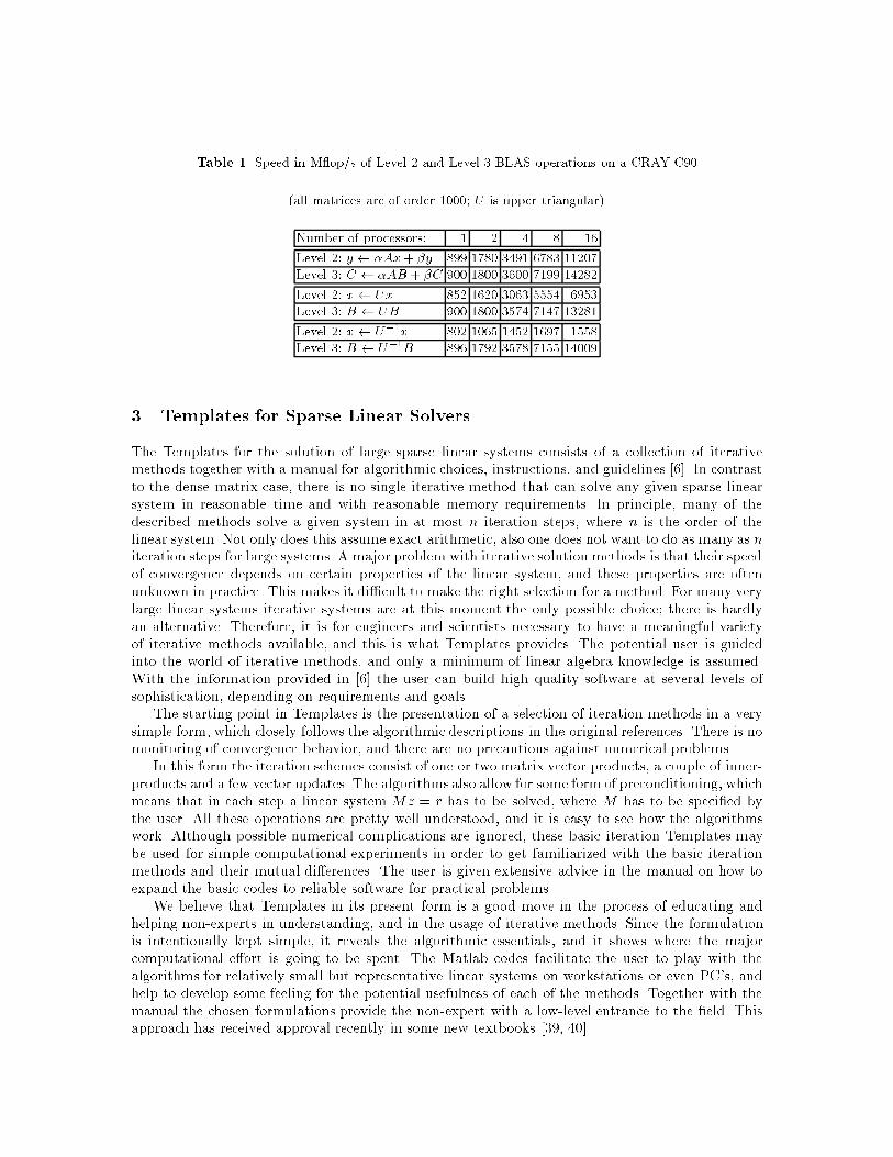
Table 1. Speed in M op/s of Level 2 and Level 3 BLAS operations on a CRAY C90

(all matrices are of order 1000; U is upper triangular)

Number of processors: 1 2 4 8 16

Level 2: y �Ax+ �y 899 1780 3491 6783 11207

Level 3: C �AB + �C 900 1800 3600 7199 14282

Level 2: x Ux 852 1620 3063 5554 6953

Level 3: B UB 900 1800 3574 7147 13281

Level 2: x U�1x 802 1065 1452 1697 1558

Level 3: B U�1B 896 1792 3578 7155 14009

3 Templates for Sparse Linear Solvers

The Templates for the solution of large sparse linear systems consists of a collection of iterative

methods together with a manual for algorithmic choices, instructions, and guidelines [6]. In contrast

to the dense matrix case, there is no single iterative method that can solve any given sparse linear

system in reasonable time and with reasonable memory requirements. In principle, many of the

described methods solve a given system in at most n iteration steps, where n is the order of the

linear system. Not only does this assume exact arithmetic, also one does not want to do as many as n

iteration steps for large systems. A major problem with iterative solution methods is that their speed

of convergence depends on certain properties of the linear system, and these properties are often

unknown in practice. This makes it di�cult to make the right selection for a method. For many very

large linear systems iterative systems are at this moment the only possible choice; there is hardly

an alternative. Therefore, it is for engineers and scientists necessary to have a meaningful variety

of iterative methods available, and this is what Templates provides. The potential user is guided

into the world of iterative methods, and only a minimum of linear algebra knowledge is assumed.

With the information provided in [6] the user can build high quality software at several levels of

sophistication, depending on requirements and goals.

The starting point in Templates is the presentation of a selection of iteration methods in a very

simple form, which closely follows the algorithmic descriptions in the original references. There is no

monitoring of convergence behavior, and there are no precautions against numerical problems.

In this form the iteration schemes consist of one or two matrix vector products, a couple of inner-

products and a few vector updates. The algorithms also allow for some form of preconditioning, which

means that in each step a linear system Mz = r has to be solved, where M has to be speci�ed by

the user. All these operations are pretty well understood, and it is easy to see how the algorithms

work. Although possible numerical complications are ignored, these basic iteration Templates may

be used for simple computational experiments in order to get familiarized with the basic iteration

methods and their mutual di�erences. The user is given extensive advice in the manual on how to

expand the basic codes to reliable software for practical problems.

We believe that Templates in its present form is a good move in the process of educating and

helping non-experts in understanding, and in the usage of iterative methods. Since the formulation

is intentionally kept simple, it reveals the algorithmic essentials, and it shows where the major

computational e�ort is going to be spent. The Matlab codes facilitate the user to play with the

algorithms for relatively small but representative linear systems on workstations or even PC's, and

help to develop some feeling for the potential usefulness of each of the methods. Together with the

manual the chosen formulations provide the non-expert with a low-level entrance to the �eld. This

approach has received approval recently in some new textbooks [39, 40].

The formulations and the notations have been chosen so that di�erences and similarities between

algorithms are easily recognized. In this respect they provide simple and easy to code algorithms,

that can serve as a yardstick with which other implementations can be compared. Templates provides

codes in Fortran, Matlab, and C. The codes are equivalent for each algorithm,and the only di�erences

in outputs may be attributed to the respective computer arithmetic. This usage of Templates makes

it easier to compare and to present results for iteration methods in publications. It is easier now to

check results which have been obtained through these standardized codes.

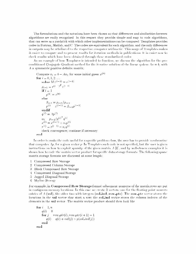
As an example of how Templates is intended to function, we discuss the algorithm for the pre-

conditioned Conjugate Gradient method for the iterative solution of the linear system Ax = b, with

A a symmetric positive de�nite matrix:

Compute r0 = b�Ax0 for some initial guess x(0)

for i = 0; 1; 2; ::::

solve Mz(i�1) = r(i�1)

�i�1 = r(i�1)Tz(i�1)

if i = 1

p(1) = z(0)

else

�i�1 = �i�1=�i�2p(i) = z(i�1) + �i�1p

(i�1)

endif

q(i) = Ap(i)

�i = �i�1=p(i)T q(i)

x(i) = x(i�1) + �ip(i)

r(i) = r(i�1) � �iq(i)

check convergence; continue if necessary

end

In order to make the code useful for a speci�c problem class, the user has to provide a subroutine

that computes Ap, for a given vector p. In Templates such code is not speci�ed, but the user is given

instructions on how to exploit sparsity of the given matrix A [6], and by well-chosen examples it is

shown how to code the matrix vector product for speci�c data storage formats. The following sparse

matrix storage formats are discussed at some length:

1. Compressed Row Storage

2. Compressed Column Storage

3. Block Compressed Row Storage

4. Compressed Diagonal Storage

5. Jagged Diagonal Storage

6. Skyline Storage

For example, in Compressed Row Storage format subsequent nonzeros of the matrix rows are put

in contiguous memory locations. In this case we create 3 vectors: one for the oating point nonzero

entries of A (val), the other two with integers (col ind, row ptr). The row ptr vector stores the

locations in the val vector that start a row; the col ind vector stores the column indexes of the

elements in the val vector. The matrix vector product should then look like

for i = 1; n

q(i) = 0

for j = row ptr(i); row ptr(i + 1) � 1

q(i) = q(i) + val(j) � p(col ind(j))

end

end

Also suggestions are supplied for coding this on parallel computers.

For some algorithms also code has to be provided that generates AT p, and this is given much

attention.

Similarly, the user has to provide a subroutine that solves the equation Mz = r for given

right-hand side r. In this respect M is called the preconditioner and the choice for an appropriate

preconditioner is left to the user. The main reason for this is that it is very di�cult, if not impossible,

to predict what a good preconditioner might be for a given problem of which little else is known

besides the fact that A is symmetric positive de�nite. In [6] an overview is given of possible choices

and semi-code for the construction of some popular preconditioners is provided, along with instruc-

tions and examples on how to code them for certain data-storage formats. A popular preconditioner

that is often used in connection with the Conjugate Gradient method is the Incomplete Cholesky

preconditioner. If we write the matrix A as A = L+D+LT (L is strictly lower diagonal,D is diag-

onal), then a simpli�ed form of the preconditioner can be written as M = (L+DC)D�1C (DC +LT ),

and in [6] formulas are given for the computation of the elements of the diagonal matrix DC . Since

the factor L is part of A, the coding for the preconditioner is not too complicated.

The other operations (inner-products and vector updates) in the algorithm are coded, in the

Fortran codes, as BLAS operations. On most modern computers these BLAS are standard available

as optimized kernels, and the user needs not to be concerned with these vector operations.

So if the user wants to have transportable code then he only needs to focus on the matrix vector

product and the preconditioner. However, there is more that the user might want to re ect on. In

the standard codes only a simple stopping criterion is provided, but in [6] a lengthy discussion is

provided on di�erent possible termination strategies and their merits. Templates for these strategies

have not yet been provided since the better of these strategies require estimates for such quantities as

kAk, or even kA�1k, and we do not know about convenient algorithms for estimating these quantities

(except possibly for the symmetric positive de�nite case). This is in contrast with dense systems,

for which e�cient estimators are available. As soon as a reliable estimating mechanisms for these

norms become known then a template can be added.

The situation for other methods, for instance Bi-CG, may be slightlymore complicated. Of course

the standard template is still simple but now the user may be facing (near) break-down situations in

actual computing. The solution for this problem is quite complicated, and the average user may not

be expected to incorporate this easily and is referred to more professional software at this moment.

A template for a cure of the break-downs would be very nice but is not planned as yet.

Also the updating for the residual vector r(i) and the approximate solution x(i) may su�er from

problems due to the use of �nite precision arithmetic. This may result into a vector r(i) that di�ers

signi�cantly from b � Ax(i), whereas these vectors should be equal in exact arithmetic. Recently,

good and reliable strategies have been suggested [34], and these are easily incorporated into the

present Templates.

At the moment the linear systems templates for iterative methods form a good starting point

for the user for the construction of useful software modules. It is anticipated that in future updates,

templates will be added for algorithmic details, such as reliable vector updating, stopping criteria,

and error monitoring. It is also conceivable that templates will be provided that help the user

to analyze the convergence behavior, and to help get more insight in characteristics of the given

problem. Most of these aspects are now covered in the Templates book, in the form of guidelines

and examples. The Templates book [6] gives an abundance of references for more background and

for all kinds of relevant details.

4 Templates for Solution of Eigenvalue Problems

To guide our eigenvalue template design, we need to have a model of what the reader wants. We

expect that a non-expert user confronted with an eigenvalue problem would be willing to supply

{ as few facts as necessary about the operator or operators whose spectral information is desired,

{ the kind of spectral information desired (including accuracy), and

{ the kind of computer available to solve it (perhaps).

In return, the user would want

{ the software to solve the problem,

{ an estimate of how long it will take to solve, and

{ a way to assess the accuracy (perhaps).

In the (likely) case that no single best algorithm exists, we expect the user would want a list of

reasonable alternatives and a discussion of the tradeo�s in time, space and accuracy among them.

For example, it might be reasonable to use a dense algorithm on a sparse problem if high accuracy

is desired, the problem is not too large, and/or the problem is to be solved just once. Much of our

e�ort will center on educating the user as to which facts must be supplied to make a decision. To

this end we have decided to categorize available methods along �ve (mostly independent) axes:

1. Mathematical Properties of the Problem,

2. Desired Spectral Information,

3. Problem Representation,

4. Available Transformations, and

5. Costs (including dependence on accuracy, computer type).

Ideally, the user would supply a \coordinate" for each of these �ve axes, thus uniquely identifying a

problem class for which we could identify a \best algorithm," software implementing it, a performance

model to predict its execution time, and a method to assess the accuracy.

Realistically, only a few regions of this �ve-dimensional space are populated with interesting

or useful algorithms, and we expect to have a more decision-tree like approach to guide the user's

expectations. The next �ve section of this paper are organized corresponding to one possible decision

tree. The �rst \level" of the tree distinguishes problems according to their mathematical properties.

The second level asks for desired spectral information, and so on.

This is not the only way to organize the decision tree. For example, a di�erent user may wish to

specify the desired spectral information later, in order to get a list of all possible algorithms relevant

to her problem. Indeed, the actual internal organization of the tree may more resemble a lattice,

since the some basic algorithms will be used many times in slightly di�erent ways. Nonetheless,

we believe these �ve axes are a good organizational tool for us to make sure we have covered all

interesting cases, or at least limit the scope of what we want in an organized way. At this point, we

invite suggestions as to the scope of our proposed project, whether we have left anything important

out, or included something of lesser importance. Brie y, we only want to include a problem type

if there is signi�cant demand, and exploiting its special features confers signi�cant performance or

accuracy advantages over using a more general purpose algorithm. We want to keep the project

small enough to come out with a reference book of at most two hundred pages (or the equivalent in

html) within 2 years.

4.1 Notation

Matrix Pencil: We will talk mostly about eigenproblems of the form (A��B)x = 0. A� �B is also

called a matrix pencil. � is an indeterminate in this latter expression, and indicates that there

are two matrices which de�ne the eigenproblem. A and B need not be square.

Eigenvalues and Eigenvectors: For almost all �xed scalar values of �, the rank of the matrix A��Bwill be constant. The discrete set of values of � for which the rank of A� �B is lower than this

constant are the eigenvalues. Let �1; :::; �k be the discrete set of eigenvalues. Some �i may be

in�nite, in which case we really consider �A�B with eigenvalue �i = 0. Nonzero vectors xi and

yi such that

Axi = �iBxi yHi A = �iyHi B;

are called a right eigenvector and a left eigenvector, respectively, where AT is the transpose of

A and AH is its conjugate-transpose. The word eigenvector alone will mean right eigenvector.

Since there are many kinds of eigenproblems, and associated algorithms, we propose some simple

top level categories to help classify them. The ultimate decision tree presented to the reader will

begin with easier concepts and questions about the eigenproblem in an attempt to classify it, and

proceed to harder questions. For the purposes of this overview, we will use rather more advanced

categories in order to be brief but precise. For background, see [23, 25, 12].

Regular and Singular Pencils: A � �B is regular if A and B are square and det(A � �B) is not

identically zero for all �; otherwise it is singular.

Regular pencils have well-de�ned sets of eigenvalues which change continuously as functions of

A and B; this is a minimal requirement to be able to compute the eigenvalues accurately, in the

absence of other constraints on A and B. Singular pencils have eigenvalues which can change

discontinuously as functions of A and B; extra information about A and B, as well as special

algorithms which use this information, are necessary in order to compute meaningful eigenvalues.

Regular and singular pencils have correspondingly di�erent canonical forms representing their

spectral decompositions. The Jordan Canonical Form of a single matrix is the best known; the

Kronecker Canonical Form of a singular pencil is the most general. More will be discussed in

section 4.3 below.

Self-adjoint and Non-self-adjoint Eigenproblems: We abuse notation to avoid confusion with the

very similar but less general notions of Hermitian and non-Hermitian: We call an eigenprob-

lem A � �B is self-adjoint if 1) A and B are both Hermitian, and 2) there is a nonsingular X

such that XAXH = �A and XBXH = �B are real and diagonal. Thus the �nite eigenvalues are

real, all elementary divisors are linear, and the only possible singular blocks in the Kronecker

Canonical Form represent a common null space of A and B. The primary source of self-adjoint

eigenproblems is eigenvalue problems in which B is known to be positive de�nite; in this case

A� �B is called a de�nite pencil. These properties lead to generally simpler and more accurate

algorithms. We classify the singular value decomposition (SVD) and its generalizations as self-

adjoint, because of the relationship between the SVD of A and the eigendecomposition of the

Hermitian matrix

�0 A

AH 0

�.

It is sometimes possible to change the classi�cation of an eigenproblem by simple transformations.

For example, multiplying a skew-Hermitian matrix A (i.e., AH = �A) by the constantp�1 makes

it Hermitian, so its eigenproblem becomes self-adjoint. Such simple transformations are very useful

in �nding the best algorithm for a problem.

Many other de�nition and notation will be introduced in section 4.3.

4.2 Level 1 of Decision Tree Mathematical Properties

We will �rst list what we plan to include in the �rst round of the project, and then what we plan

not to include.

What we plan to include The following description is very terse. The user will see a more ex-

tended description of each problem, including common synonyms.

1. Hermitian eigenproblem A� �I

2. Non-Hermitian eigenproblem A � �I

3. Generalized de�nite eigenproblem A � �B, where A = AH , B = BH > 0

4. Generalized Hermitian eigenproblem A� �B, where A = AH , B = BH

5. Generalized non-Hermitian eigenproblem A� �B, where B = BH > 0

6. Generalized non-Hermitian Eigenproblem A� �B

7. Quadratic �2A+ �B + C or higher degree ��iAi eigenvalue problems

8. Singular Value Decomposition (SVD) of a single general matrix A

9. Generalized SVD of A and B

10. Other eigenvalue problems

Note that this list does include all the possible variations hinted at in the previous section; these

will appear as the user traverses the tree. For example, there will be cross references to other, better

algorithms in cases for which simple transformations permit their use. Here are some examples:

{ Under \Hermitian eigenproblem A� �I": If A = BBH , the user will be advised to consider the

SVD of B.

{ Under \Generalized Hermitian eigenproblem": If A = AH and B = BH , and the user knows real

constants � and � such that �A + �B is positive de�nite, the user will be advised to consider

the de�nite eigenproblem A � �(�A + �B).

{ Under \Non-Hermitian eigenproblem A � �I": If B = �SAS�1 is Hermitian for known, simple

� and S, the user will be advised to consider the eigenproblem for B.

{ Under \SVD of A": If A = BC�1, the user will be advised to consider the quotient SVD of B

and C.

{ Under \Quadratic �2A+ �B +C or higher degree ��iAi eigenvalue problems", the user will be

advised to consider the linearization of problem to a matrix pencil eigenvalue problem.

{ Under \Other eigenvalue problems", the user will see some other related eigenvalue problems,

such as

� Updating eigendecompositions

� Polynomial zero �nding

� Rank revealing QR decomposition

What we plan not to include Some of them we may include, provided there is su�cient demand.

Mostly, we would limit ourselves to literature references.

{ There is a variety of \non-linear" eigenproblems which can be linearized in various ways and

converted to the above problems

1. Rational problems A(�)

2. General nonlinear problems A(�)

3. Polynomial system zero �nding

{ The SVD can be used to solve a variety of least squares problems, and these may best be solved

by representing the SVD in \factored" form. These factored SVD algorithms are somewhat com-

plicated and hard to motivate without the least squares application, but there are a great many

least squares problems, but including too many of them (beyond references to the literature)

would greatly expand the scope of this project. The same comments apply to the generalized

SVD, of which there are even more variations.

{ Eigenproblems from systems and control. There is a large source of eigenproblems, many of

which can be reduced to �nding certain kinds of spectral information about possibly singular

pencils A � �B. These problems arise with many kinds of special structures, many of which

have been exploited in special packages, some of them can be solved by general algorithms. For

example, solutions of Riccati equations are often reduced to eigenproblems. A comprehensive

treatment of these problems would greatly expand the scope of the book, but including some

treatment seems important.

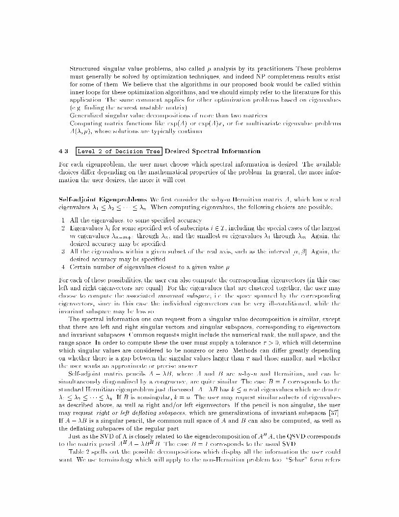
{ Structured singular value problems, also called �-analysis by its practitioners These problems

must generally be solved by optimization techniques, and indeed NP-completeness results exist

for some of them. We believe that the algorithms in our proposed book would be called within

inner loops for these optimization algorithms, and we should simply refer to the literature for this

application. The same comment applies for other optimization problems based on eigenvalues

(e.g. �nding the nearest unstable matrix).

{ Generalized singular value decompositions of more than two matrices

{ Computing matrix functions like exp(A) or exp(A)x, or for multivariate eigenvalue problems

A(�; �), whose solutions are typically continua.

4.3 Level 2 of Decision Tree Desired Spectral Information

For each eigenproblem, the user must choose which spectral information is desired. The available

choices di�er depending on the mathematical properties of the problem. In general, the more infor-

mation the user desires, the more it will cost.

Self-adjoint Eigenproblems We �rst consider the n-by-n Hermitian matrix A, which has n real

eigenvalues �1 � �2 � � � � � �n. When computing eigenvalues, the following choices are possible:

1. All the eigenvalues, to some speci�ed accuracy.

2. Eigenvalues �i for some speci�ed set of subscripts i 2 I, including the special cases of the largestm eigenvalues �n�m+1 through �n, and the smallest m eigenvalues �1 through �m. Again, the

desired accuracy may be speci�ed.

3. All the eigenvalues within a given subset of the real axis, such as the interval [�; �]. Again, the

desired accuracy may be speci�ed.

4. Certain number of eigenvalues closest to a given value �.

For each of these possibilities, the user can also compute the corresponding eigenvectors (in this case

left and right eigenvectors are equal). For the eigenvalues that are clustered together, the user may

choose to compute the associated invariant subspace, i.e. the space spanned by the corresponding

eigenvectors, since in this case the individual eigenvectors can be very ill-conditioned, while the

invariant subspace may be less so.

The spectral information one can request from a singular value decomposition is similar, except

that there are left and right singular vectors and singular subspaces, corresponding to eigenvectors

and invariant subspaces. Common requests might include the numerical rank, the null space, and the

range space. In order to compute these the user must supply a tolerance � > 0, which will determine

which singular values are considered to be nonzero or zero. Methods can di�er greatly depending

on whether there is a gap between the singular values larger than � and those smaller, and whether

the user wants an approximate or precise answer.

Self-adjoint matrix pencils A � �B, where A and B are n-by-n and Hermitian, and can be

simultaneously diagonalized by a congruence, are quite similar. The case B = I corresponds to the

standard Hermitian eigenproblem just discussed. A��B has k � n real eigenvalues which we denote

�1 � �2 � � � � � �k. If B is nonsingular, k = n. The user may request similar subsets of eigenvalues

as described above, as well as right and/or left eigenvectors. If the pencil is non-singular, the user

may request right or left de ating subspaces, which are generalizations of invariant subspaces [37].

If A� �B is a singular pencil, the common null-space of A and B can also be computed, as well as

the de ating subspaces of the regular part.

Just as the SVD of A is closely related to the eigendecomposition of AHA, the QSVD corresponds

to the matrix pencil AHA� �BHB. The case B = I corresponds to the usual SVD.

Table 2 spells out the possible decompositions which display all the information the user could

want. We use terminology which will apply to the non-Hermitian problem too. \Schur" form refers

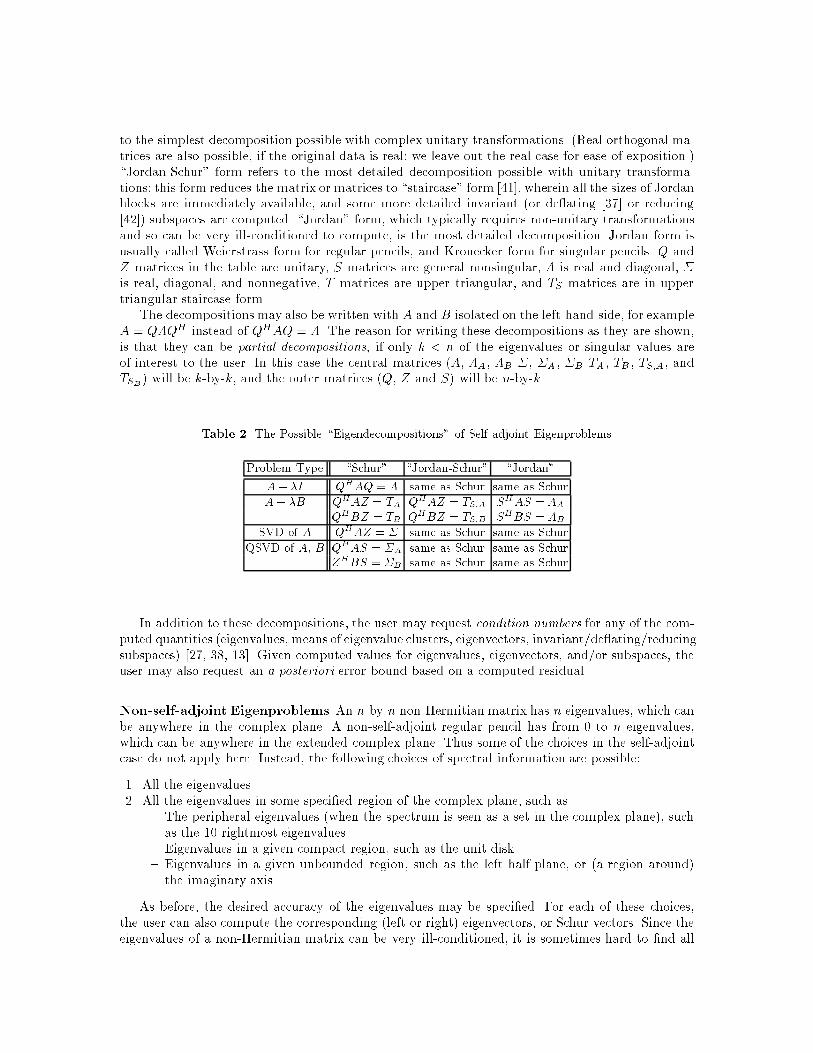
to the simplest decomposition possible with complex unitary transformations. (Real orthogonal ma-

trices are also possible, if the original data is real; we leave out the real case for ease of exposition.)

\Jordan-Schur" form refers to the most detailed decomposition possible with unitary transforma-

tions; this form reduces the matrix or matrices to \staircase" form [41], wherein all the sizes of Jordan

blocks are immediately available, and some more detailed invariant (or de ating [37] or reducing

[42]) subspaces are computed. \Jordan" form, which typically requires non-unitary transformations

and so can be very ill-conditioned to compute, is the most detailed decomposition. Jordan form is

usually called Weierstrass form for regular pencils, and Kronecker form for singular pencils. Q and

Z matrices in the table are unitary, S matrices are general nonsingular, � is real and diagonal, �

is real, diagonal, and nonnegative, T matrices are upper triangular, and TS matrices are in upper

triangular staircase form.

The decompositions may also be written with A and B isolated on the left-hand-side, for example

A = Q�QH instead of QHAQ = �. The reason for writing these decompositions as they are shown,

is that they can be partial decompositions, if only k < n of the eigenvalues or singular values are

of interest to the user. In this case the central matrices (�, �A, �B �, �A, �B TA, TB , TS;A, and

TSB ) will be k-by-k, and the outer matrices (Q, Z and S) will be n-by-k.

Table 2. The Possible \Eigendecompositions" of Self-adjoint Eigenproblems

Problem Type \Schur" \Jordan-Schur" \Jordan"

A� �I QHAQ = � same as Schur same as Schur

A� �B QHAZ = TA QHAZ = TS;A SHAS = �A

QHBZ = TB QHBZ = TS;B SHBS = �B

SVD of A QHAZ = � same as Schur same as Schur

QSVD of A, B QHAS = �A same as Schur same as Schur

ZHBS = �B same as Schur same as Schur

In addition to these decompositions, the user may request condition numbers for any of the com-

puted quantities (eigenvalues, means of eigenvalue clusters, eigenvectors, invariant/de ating/reducing

subspaces) [27, 38, 13]. Given computed values for eigenvalues, eigenvectors, and/or subspaces, the

user may also request an a posteriori error bound based on a computed residual.

Non-self-adjoint Eigenproblems An n-by-n non-Hermitian matrix has n eigenvalues, which can

be anywhere in the complex plane. A non-self-adjoint regular pencil has from 0 to n eigenvalues,

which can be anywhere in the extended complex plane. Thus some of the choices in the self-adjoint

case do not apply here. Instead, the following choices of spectral information are possible:

1. All the eigenvalues.

2. All the eigenvalues in some speci�ed region of the complex plane, such as

{ The peripheral eigenvalues (when the spectrum is seen as a set in the complex plane), such

as the 10 rightmost eigenvalues.

{ Eigenvalues in a given compact region, such as the unit disk.

{ Eigenvalues in a given unbounded region, such as the left half plane, or (a region around)

the imaginary axis.

As before, the desired accuracy of the eigenvalues may be speci�ed. For each of these choices,

the user can also compute the corresponding (left or right) eigenvectors, or Schur vectors. Since the

eigenvalues of a non-Hermitian matrix can be very ill-conditioned, it is sometimes hard to �nd all

eigenvalues within a given region with certainty. For eigenvalues that are clustered together, the user

may choose to estimate the mean of the cluster, or even the �-pseudospectrum, the smallest region

in the complex plane which contains all the eigenvalues of all matrices B di�ering from the given

matrix A by at most �: kA�Bk � �. The user may also choose to compute the associated invariant

(or de ating or reducing) subspaces (left or right) instead of individual eigenvectors. However, due

to the potential ill-conditioning of the eigenvalues, there is no guarantee that the invariant subspace

will be well-conditioned.

A singular pencil has a more complicated eigenstructure, as de�ned by the Kronecker Canonical

Form, a generalization of the Jordan Canonical Form [23, 41]. Instead of invariant or de ating

subspaces, we say a singular pencil has reducing subspaces.

Table 3 spells out the possibilities. In addition to the notation used in the last section, U matri-

ces denote generalized upper triangular (singular pencils only), US matrices are generalized upper

triangular in staircase form (singular pencils only), J is in Jordan form, and K is in Kronecker form.

As before, these can be partial decompositions, when Q, Z, SL and SR are n-by-k instead of n-by-n.

Table 3. The Possible \Eigendecompositions" of Non-self-adjoint Eigenproblems

Problem Type \Schur" \Jordan-Schur" \Jordan"

A� �I QHAQ = T QHAQ = TS S�1AS = J

A� �B, regular QHAZ = TA QHAZ = TS;A S�1

L ASR = JA

QHBZ = TB QHBZ = TS;B S�1L BSR = JB

A� �B, singular QHAZ = UA QHAZ = US;A S�1L ASR = KA

QHBZ = UB QHBZ = US;B S�1L BSR = KB

In addition to these decompositions, the user may request condition numbers for any of the com-

puted quantities (eigenvalues, means of eigenvalue clusters, eigenvectors, invariant/de ating/reducing

subspaces). Given computed values for eigenvalues, eigenvectors, and/or subspaces, the user may also

request an a posteriori error bound based on a computed residual.

4.4 Level 3 of Decision Tree Problem Representation

First we discuss the type of individual matrix or operator entries. The simplest distinction is between

real and complex data. The issues are speed (real arithmetic is faster than complex), storage (real

numbers require half the storage of complex numbers), code complexity (some algorithms simplify

greatly if we can do complex arithmetic), and stability (real arithmetic can guarantee complex

conjugate eigenvalues of real matrices). The distinction between single and double precision, which

clearly a�ects space, will be discussed again as an accuracy issue.

Given the type of individual operator entries, we must distinguish the overall structure of the

operator. Here is our list. Two letter abbreviations (like GE) refer to matrix types supported by

LAPACK [1, Table 2.1].

{ Dense matrices

� General (GE)

� Hermitian, with only upper or lower half de�ned (SY or HE)

� Hermitian, packed into half the space (SP or HP)

{ Matrices depending systematically on O(n) data.

� Band matrices

� Bidiagonal matrices, stored as two arrays (BD)

� Tridiagonal matrices, stored as two or three arrays (ST, GT)

� Wider band matrices (GB, SB, HB)

� Band matrices with bulges (\look ahead" matrices)

� Arrow, Toeplitz, Hankel, Circulant, and Companion matrices

� Diagonal + rank-1 matrices, band + low rank matrices

{ Sparse matrices, or those depending less systematically on o(n2) data. It turns out that the

relevant classi�cation is by the operations that can be performed on the operators represented,

not the details of the representation. This will be clearer in Section 4.5.

� can solve the linear system (A� �B)x = b

� Matrix-vector multiplication possible y = Ax (and y = AHx) (this includes, for example,

\dense" integral operators which have fast algorithms for performing y = Ax.)

� under SVD or GSVD, possible to factor AAH � �BBH or AHA � �BHB, or

�0 A

AH 0

��

�

�I 0

0 BHB

�, perhaps shifted

There are many more special structures, often arising from control theory, such as unitary or-

thogonal matrices represented by their Schur parameters. Until we hear of a large demand for such

problems, we do not plan to include them, other than as literature references. For the same reason

we also do not plan to include algorithms for quaternion matrices, or matrices with rational entries,

which are more properly included in the domain of symbolic computation.

4.5 Level 4 of Decision Tree Available Operations

The choice between di�erent methods very much depends on which of these operations one has

available at a reasonable cost. We list the major ones in decreasing order of power:

{ For those methods, which do not generally require user tuning for accuracy and reliability and

has predictable cost and performance.

� Some special matrices, such as bidiagonals or diagonal + rank-1 matrices, have special algo-

rithms designed especially for them. Many good implementations are available [1].

� Similarity transformations S�1AS can be applied to matrices A of reasonable size, stored

as two dimensional arrays, or in a dense band structure. (For pencils A� �B, we would use

equivalence transformations S�1L ASR � �S�1L BSR instead). Many of these algorithms have

good implementations available [1]. Some of them (such as sign function based algorithms

[5]) are currently being implemented. When good \black-box" implementations exist, they

will not be described in detailed templates. We will however indicate when they are to be

preferred over the iterative methods, which are the main theme of this collection.

{ For those methods, which generally require user tuning

� Multiplication of a vector x by a shifted-and-inverted operator, y = (A � �I)�1x or y =

(A � �B)�1Bx for a given vector x, lets us quickly compute the eigenvalues closest to the

shift �. This operation may be implemented with an explicit triangular factorization

A� �B = PLU

e.g. as a part of an FEM (�nite element method) package, but any other implementationmay

also be used, such as those based on multigrid or more specialized methods. It is also possible

to use an iterative solver which only uses multiplication by A (or A and B) internally, but

this may not be superior to other methods discussed below.

� If the shift � is restricted, say to 0, then we will be restricted to e�ciently �nding eigenvalues

closest to zero, and will need more iterations to �nd any but the few smallest eigenvalues.

� If only B is factorizable, e.g. if B = I, so that we can only multiply vectors by AB�1, we

will be restricted to e�ciently �nding the peripheral eigenvalues, i.e. those eigenvalues near

the \edges" of the spectrum, when the spectrum is seen as a set in the complex plane.

If, in a special purpose method, it is possible to multiply a vector by AH in addition to A, or

possibly y = (A � �I)�Hx or y = BH (A � �B)�Hx, depending on the situation, then a broader,

more powerful class of algorithms are available.

Sometimes it is signi�cantly cheaper to apply the operator to a set of vectors rather than just

1 vector at a time. This can happen because of memory hierarchy e�ects. There are algorithms to

exploit this behavior.

The worst case is when the only operation we can perform is multiplication of a vector by A

(and possibly B). But algorithms are available in this case too.

Not only the matrix-vector operations but also the vector algebra needs special consideration. In

all the algorithms that we will consider, only two di�erent vector operations have to be applied to

vectors of length n, dot products and the addition of a multiple of one vector to another, axpy to

use terminology from the BLAS. These operations may be implemented on distributed processors

in a way that is appropriate for the application or the computer at hand. In some cases a vector is

not even represented as an array of numbers, but stands for a function represented in e.g. a �nite

element or wavelet basis. Then user-supplied routines for dot products and axpy will replace the

basic vector operations in our templates.

4.6 Basic Iterative Algorithms

The following basic algorithms for sparse eigenproblems will be included.

{ Simultaneous iteration methods

{ Arnoldi methods

{ Lanczos methods

{ Davidson methods

{ Re�nement methods

{ Trace minimization (self-adjoint case only)

This list is not exhaustive, and we are actively looking for other algorithms. Also, some common

methods may classi�ed in several ways. For example, simultaneous iteration and block Arnoldi with

an immediate restart are identical. These categories are not meant to be mutually exclusive, but to

be helpful to the user. We will include some older but commonly used methods, just to be able to

advise the user to use more powerful alternatives, and for experimental purposes.

Arnoldi and Lanczos methods are Krylov subspaces based techniques. These methods may con-

verge very fast in combination with shifted-and-inverted operators, which means that (A��I)�1 hasto be used in matrix vector products in each iteration step. If only approximations for (A � �I)�1

are available then Davidson's method can be used as an acceleration technique for the inexact shift-

and-invert operations. Approximations for (A � �I)�1 can be computed from a preconditioner for

A� �I or by a few steps of a (preconditioned) iterative method [35].

Trace minimization is suitable for self-adjoint problems, and uses optimization techniques like

conjugate gradients to �nd the k smallest eigenvalues.

There is unfortunately no simple way to identify the best algorithm and choice of options to

the user. The more the user discovers about the problem (such as approximate eigenvalues), the

better a choice can be made. In the common situation where the user is solving a sequence of similar

problems, this is quite important.

There is also unfortunately no inexpensive way to provide a guarantee that all eigenvalues in a

region have been found, when the problem is not self-adjoint. For Hermitian eigenvalue problems by

factoring certain translations of A by the identity, it is possible to guarantee that all eigenvalues in a

region have been found. In the non-Hermitian case, this same task is accomplished by a vastly more

expensive technique called a Nyquist plot (i.e. compute the winding number). However, depending

on the problem, there are methods to help increase one's con�dence that all eigenvalues have been

found.

4.7 Cost Issues

As stated above, the user would ideally like a simple formula, or perhaps a program, that would

predict the running time as a function of a few simple facts about the problem to be solved, and

the computer to be used to solve it. This implies that we need to build performance models for all

the algorithms we provide. Realistically, for some dense algorithms we will be able to give operation

counts, dependent on the size and mathematical properties of the problem to be solved, the infor-

mation desired by the user, and perhaps some rough properties of the operator, like the clustering of

the spectrum. For sparse problems, we can do the same for the inner loop of the iteration, counting

operations like matrix-factorizations, matrix-vector multiplies, dot products, saxpys, and so on.

For particular machines, we can provide Matlab scripts to actually estimate running times in

terms of a few machine parameters, likemega op rate (for the 3 levels of BLAS), number of processors

and communication costs (for parallel machines), matrix dimension, layout (on parallel machines),

information desired by the user, and so on. There are two basic approaches to producing such

performance models (hybrids are possible too). The �rst is intrinsic, which uses operation counts

plus simpler models for the costs of each operation (BLAS operations and communication), and

the second is extrinsic, which simply does curve �tting of benchmark runs. Intrinsic models are

more di�cult to produce, may be less accurate in certain extreme cases, but are more exible and

illuminating than extrinsic models.

4.8 Accuracy Issues

As usual in numerical linear algebra, we will use the backward error analysis model to assess the

accuracy of the results. We will �rst give perturbation theorems that tell how much a perturbation

of the data, in this case matrix elements, will change the results, eigenvalues, singular values and

vectors. We will also provide a posteriori methods to measure the backward error for computed

solutions.

In the simplest cases, the perturbation theorems give a bound for the perturbation of the eigen-

values as a multiple of the perturbation of the matrix elements. The multiplier is called a condition

number. For eigenvectors we also need information about the distance between the di�erent eigen-

values, as well as the angles between left and right eigenvectors. In degenerate cases, the best we

can get is an asymptotic series, possibly involving fractional powers of the perturbation.

We will discuss what to do when a simple condition number based bound is not practical. If

we do not have good bounds for individual eigenvectors, then a better conditioned invariant (or

de ating or reducing) subspace of higher dimension may be available. We can also derive a bound

for the norm of the resolvent and �nd pseudospectra.

For iterative algorithms a posteriori methods are used to compute the backward error, often

using computed residuals. It is possible to compute, or at least estimate, the residual during the

computation as part of monitoring for convergence.

We will show when stronger results as e.g. small relative error bounds for small eigenvalues exist.

This is of importance, specially when an ill conditioned matrix comes from the discretization of a

well conditioned continuous problem.

4.9 Format of Results

As stated at the beginning of Section 4, the user would ideally want to be asked a few questions

about his or her problem, and in return get summary of the right algorithm to use, a pointer to

corresponding software, and performance and accuracy predictions. In addition to the conventional

book format in which such information could be presented, we plan to explore the use of a hypertext

interface to let the user browse through the information, and traverse the underlying decision tree.

Both \black boxes" as in LAPACK and \templates" will be possible recommendations at the bottom

of the decision tree. Black boxes will be brie y described, but not in su�cient detail to reproduce

a good implementation (which is why they are black boxes!). Templates will be made available in

pseudocode, Matlab, and Fortran, as they were in the prior Templates book. If there is strong feeling

that C, C++, or Fortran 90 should also be used, we would like to hear it (but note that we do not

have the resources to recode LAPACK in Fortran-90 or C++, although wrappers are possible). We

hope to assemble a set of test cases, and evaluate the algorithms we suggest on these test cases. The

test cases should demonstrate both typical and extreme behaviors of the algorithms.

References

1. E. Anderson, Z. Bai, C. Bischof, J. Demmel, J. Dongarra, J. Du Croz, A. Greenbaum, S. Hammarling,A. McKenney, S. Ostrouchov, and D. Sorensen. LAPACK Users' Guide, Release 2.0. SIAM, Philadel-

phia, 1995. 324 pages. URL http://www.netlib.org/lapack/lug/lapack lug.html.

2. E. Anderson and J. Dongarra. Results from the initial release of LAPACK. Technical Report LAPACKworking note 16, Computer Science Department, University of Tennessee, Knoxville, TN, 1989.

3. E. Anderson and J. Dongarra. Evaluating block algorithm variants in LAPACK. Technical Report

LAPACK working note 19, Computer Science Department, University of Tennessee, Knoxville, TN,1990.

4. Z. Bai. Progress in the numerical solution of the nonsymmetric eigenvalue problem, 1993. To appear in

J. Num. Lin. Alg. Appl.5. Z. Bai and J. Demmel. Design of a parallel nonsymmetric eigenroutine toolbox, Part I. In Proceedings of

the Sixth SIAM Conference on Parallel Proceeding for Scienti�c Computing. SIAM, 1993. Long version

available as UC Berkeley Computer Science report all.ps.Z via anonymous ftp from tr-ftp.cs.berkeley.edu,directory pub/tech-reports/csd/csd-92-718.

6. R. Barrett, M. Berry, T. Chan, J. Demmel, J. Donato, J. Dongarra, V. Eijkhout, V. Pozo, Romime C.,

and H. van der Vorst. Templates for the solution of linear systems: Building blocks for iterative methods.SIAM, 1994. URL http://www.netlib.org/templates/templates.ps.

7. R. Boisvert. The architecture of an intelligent virtual mathematical software repository system. Math-

ematics and Computers in Simulation, 36:269{279, 1994.8. J. Choi, J. J. Dongarra, R. Pozo, and D. W. Walker. ScaLAPACK: A scalable linear algebra library for

distributed memory concurrent computers. In Proceedings of the Fourth Symposium on the Frontiers of

Massively Parallel Computation, pages 120{127. IEEE Computer Society Press, 1992.9. J. Choi, J. J. Dongarra, and D. W. Walker. The design of scalable software libraries for distributed

memory concurrent computers. In J. J. Dongarra and B. Tourancheau, editors, Environments and Tools

for Parallel Scienti�c Computing. Elsevier Science Publishers, 1993.10. D. E. Culler, A. Dusseau, S. C. Goldstein, A. Krishnamurthy, S. Lumetta, T. von Eicken, and K. Yelick.

Introduction to Split-C: Version 0.9. Technical report, Computer Science Division { EECS, University

of California, Berkeley, CA 94720, February 1993.11. J. Cullum and R. A. Willoughby. Lanczos algorithms for large symmetric eigenvalue computations.

Birkha�user, Basel, 1985. Vol.1, Theory, Vol.2. Program.

12. J. Demmel. Berkeley Lecture Notes in Numerical Linear Algebra. Mathematics Department, Universityof California, 1993. 215 pages.

13. J. Demmel and B. K�agstr�om. The generalized Schur decomposition of an arbitrary pencil A � �B:

Robust software with error bounds and applications. Parts I and II. ACM Trans. Math. Soft., 19(2),June 1993.

14. J. Demmel. LAPACK: A portable linear algebra library for supercomputers. In Proceedings of the 1989IEEE Control Systems Society Workshop on Computer-Aided Control System Design, December 1989.

15. J. J. Dongarra. Increasing the performance of mathematical software through high-level modularity. In

Proc. Sixth Int. Symp. Comp. Methods in Eng. & Applied Sciences, Versailles, France, pages 239{248.North-Holland, 1984.

16. J. J. Dongarra, J. R. Bunch, C. B. Moler and G. W. Stewart. LINPACK Users' Guide. SIAM Press,

1979.17. J. J. Dongarra. LAPACK Working Note 34: Workshop on the BLACS. Computer Science Dept. Tech-

nical Report CS-91-134, University of Tennessee, Knoxville, TN, May 1991.

18. J. J. Dongarra, J. Du Croz, S. Hammarling, and I. Du�. A set of level 3 basic linear algebra subprograms.

ACM Transactions on Mathematical Software, 16(1):1{17, 1990.

19. J. J. Dongarra, J. Du Croz, S. Hammarling, and R. Hanson. An extended set of Fortran basic linear

algebra subroutines. ACM Transactions on Mathematical Software, 14(1):1{17, March 1988.

20. J. J. Dongarra and R. A. van de Geijn. LAPACK Working Note 37: Two-dimensional basic linear al-

gebra communication subprograms. Computer Science Department, University of Tennessee, Knoxville,

TN, October 1991.

21. J. Dongarra and E. Grosse. Distribution of mathematical software via electronic mail. Communications

of the ACM, 30(5):403{407, July 1987. URL http://www.netlib.org/.

22. E. W. Felten and S. W. Otto. Coherent parallel C. In G. C. Fox, editor, Proceedings of the Third

Conference on Hypercube Concurrent Computers and Applications, pages 440{450. ACM Press, 1988.

23. F. Gantmacher. The Theory of Matrices, Vol. II (transl.). Chelsea, New York, 1959.24. B. S. Garbow, J. M. Boyle, J. J. Dongarra, and C. B. Moler. Matrix Eigensystem Routines { EISPACK

Guide Extension, Volume 51 of Lecture Notes in Computer Science. Springer-Verlag, Berlin, 1977.25. G. Golub and C. Van Loan. Matrix Computations. Johns Hopkins University Press, Baltimore, MD,

2nd edition, 1989.

26. R. W. Hockney and C. R. Jesshope. Parallel Computers. Adam Hilger Ltd., Bristol, UK, 1981.27. T. Kato. Perturbation Theory for Linear Operators. Springer Verlag, Berlin, 2 edition, 1980.

28. C. Lawson, R. Hanson, D. Kincaid, and F. Krogh. Basic Linear Algebra Subprograms for Fortran usage.

ACM Trans. Math. Soft., 5:308{323, 1979.29. A. Packard, M. Fan, and J. Doyle. A power method for the structured singular value. In IEEE Conf.

on Decision and Control, pages 2132{2137, 1988.

30. B. Parlett. The Symmetric Eigenvalue Problem. Prentice Hall, Englewood Cli�s, NJ, 1980.31. B. Parlett. The software scene in the extraction of eigenvalues from sparse matrices. SIAM J. Sci. Stat.

Comp., 5:590{604, 1984.

32. W.H. Press, B.P. Flannery, S.A. Teukolsky, and W.T. Vetterling. Numerical Recipes in C. CambridgeUniversity Press, Cambridge, UK, 1991.

33. Y. Saad. Numerical methods for large eigenvalue problems. Manchester University Press, 1992.

34. G. Sleijpen and H. van der Vorst. Reliable updated residuals in hybrid Bi-CG methods. Preprint 886,Utrecht University, the Netherlands, 1994. to appear in Computing.

35. G. Sleijpen and H. van der Vorst. A Jacobi-Davidson iteration method for linear eigenvalue problems.

Preprint 856 (revised), Utrecht University, the Netherlands, 1995 . to appear in SIMAX.36. B. T. Smith, J. M. Boyle, J. J. Dongarra, B. S. Garbow, Y. Ikebe, V. C. Klema, and C. B. Moler. Matrix

Eigensystem Routines { EISPACK Guide, Volume 6 of Lecture Notes in Computer Science. Springer-

Verlag, Berlin, 1976.37. G. W. Stewart. Error and perturbation bounds for subspaces associated with certain eigenvalue prob-

lems. SIAM Review, 15(4):727{764, Oct 1973.

38. G. W. Stewart and J.-G. Sun. Matrix Perturbation Theory. Academic Press, New York, 1990.39. C. �Uberhuber. Computer-Numerik, Part 1 and 2, Springer Verlag, Berlin, etc, 1995.

40. A.J. van der Steen (ed). Aspects of Computational Science. NCF, Den Haag, the Netherlands, 1995.

41. P. Van Dooren. The computation of Kronecker's canonical form of a singular pencil. Lin. Alg. Appl.,27:103{141, 1979.

42. P. Van Dooren. Reducing subspaces: De�nitions, properties and algorithms. In B. K�agstr�om and

A. Ruhe, editors, Matrix Pencils, pages 58{73. Springer-Verlag, Berlin, 1983. Lecture Notes in Mathe-matics, Vol. 973, Proceedings, Pite Havsbad, 1982.

43. J. H. Wilkinson. The Algebraic Eigenvalue Problem. Oxford University Press, Oxford, 1965.

44. J. Wilkinson and C. Reinsch. Handbook for Automatic Computation: Volume II - Linear Algebra.Springer-Verlag, New York, 1971.

45. P. Young, M. Newlin, and J. Doyle. Practical computation of the mixed � problem. In Proceedings of

the American Control Conference, pages 2190{2194, 1994.

This article was processed using the LaTEX macro package with LLNCS style