temporal data mining approaches for sustainable chiller

34

Temporal Data Mining Approaches for Sustainable ChillerManagement in Data Centers

DEBPRAKASH PATNAIK, Virginia TechMANISH MARWAH, HP LabsRATNESH K. SHARMA, NEC LabsNAREN RAMAKRISHNAN, Virginia Tech

Practically every large IT organization hosts data centers—a mix of computing elements, storage systems,networking, power, and cooling infrastructure—operated either in-house or outsourced to major vendors. Asignificant element of modern data centers is their cooling infrastructure, whose efficient and sustainableoperation is a key ingredient to the “always-on” capability of data centers. We describe the design andimplementation of CAMAS (Chiller Advisory and MAnagement System), a temporal data mining solutionto mine and manage chiller installations. CAMAS embodies a set of algorithms for processing multivariatetime-series data and characterizes sustainability measures of the patterns mined. We demonstrate three keyingredients of CAMAS—motif mining, association analysis, and dynamic Bayesian network inference—thathelp bridge the gap between low-level, raw, sensor streams, and the high-level operating regions and featuresneeded for an operator to efficiently manage the data center. The effectiveness of CAMAS is demonstratedby its application to a real-life production data center managed by HP.

Categories and Subject Descriptors: H.2.8 [Database Management]: Database Applications—Data mining;K.6.2 [Management of Computing and Information Systems]: Installation Management—Computingequipment management

General Terms: Algorithms, Experimentation, Measurement, Management, Reliability

Additional Key Words and Phrases: Data centers, chillers, clustering, motifs, frequent episodes, sustainability

ACM Reference Format:Patnaik, D., Marwah, M., Sharma, R. K., and Ramakrishnan, N. 2011. Temporal data mining approachesfor sustainable chiller management in data centers. ACM Trans. Intell. Syst. Technol. 2, 4, Article 34 (July2011), 29 pages.DOI = 10.1145/1989734.1989738 http://doi.acm.org/10.1145/1989734.1989738

1. INTRODUCTION

Modern IT infrastructure is ubiquitous, especially in the services sector that requires“always-on” capability. Practically every large IT organization hosts data centers, oper-ated either in-house or outsourced to major vendors. Over the last decade, data centershave grown from housing a few hundred multiprocessor systems to tens of thousandsof individual servers today. This growth has been accompanied with steep increasesin power density, resulting in higher heat dissipation, and thus increasing both power

Authors’ addresses: D. Patnaik, Department of Computer Science and Application, Virginia Tech, 1251Progress Street NW, Apt 4900G, Blacksburg, VA 24060; email: [email protected]; M. Marwah, HP Labs, 3000Hanover Street, Palo Alto, CA 94304-1185; R. K. Sharma, Department of Energy Management, NEC Labs,4 Independence Way, Suite 200, Princeton, NJ 08540; N. Ramakrishnan, Department of Computer Scienceand Application, Virginia Tech, Blacksburg, VA 24060.Permission to make digital or hard copies of part or all of this work for personal or classroom use is grantedwithout fee provided that copies are not made or distributed for profit or commercial advantage and thatcopies show this notice on the first page or initial screen of a display along with the full citation. Copyrights forcomponents of this work owned by others than ACM must be honored. Abstracting with credit is permitted.To copy otherwise, to republish, to post on servers, to redistribute to lists, or to use any component of thiswork in other works requires prior specific permission and/or a fee. Permissions may be requested fromPublications Dept., ACM, Inc., 2 Penn Plaza, Suite 701, New York, NY 10121-0701 USA, fax +1 (212)869-0481, or [email protected]© 2011 ACM 2157-6904/2011/07-ART34 $10.00DOI 10.1145/1989734.1989738 http://doi.acm.org/10.1145/1989734.1989738

ACM Transactions on Intelligent Systems and Technology, Vol. 2, No. 4, Article 34, Publication date: July 2011.

34:2 D. Patnaik et al.

and cooling costs. According to the EPA, U.S. data centers have become energy hogsand their continued growth is expected to demand the construction of 10 new powerplants by 2011 [Koomey 2008a, 2008b; Kaplan et al. 2008]. One news report [Leake andWoods 2009], perhaps alarmist, claims that a single Web search query can use up to halfthe equivalent energy of boiling a kettle of water! Globally, data centers currently con-sume 1–2% of the world’s electricity [Vanderbilt 2009] and are already responsible formore CO2 emissions than entire countries such as Argentina or The Netherlands. Ifthese trends hold, data center emissions are expected to quadruple by 2020 [Kaplanet al. 2008] and some estimates expect the carbon footprint of cloud computing tosurpass aviation [Koomey 2008a].

Data centers constitute a mix of computing elements, networking infrastructure,storage systems along with power management and cooling capabilities all of whichcontribute to energy inefficiency. A plethora of approaches are hence available to curtailenergy usage in each of the different data center subsystems and achieve sustainabledata centers. For instance, huge inefficiencies abound in average server usage (believedto be in the single digits -to- at most 10–15%), and thus one approach to achieve greenerIT is to use virtualization and migration to automatically provision new systems asdemand spikes and consolidate applications when demand falls. A lot of prior work hasfocused on a data center’s cooling infrastructure, which consumes anywhere between30% to 50% of the total power consumption of a data center. Within the cooling infras-tructure, most of the energy is spent on chillers, which refrigerate the coolant, typicallywater, used to extract heat from the equipment in the data center. Dynamic manage-ment of an ensemble of chiller units [Patnaik et al. 2009b] in response to varying loadcharacteristics is an effective strategy to make a data center more energy efficient.There are even end-to-end methodologies proposed [Sharma et al. 2008] that trackinefficiencies at all levels of the IT infrastructure “stack” and derive overall measuresof the efficiency of energy flow during data center operation.

A key problem is the unavailability, inadequacy, or infeasibility of theoretical modelsor “first principles” methodologies to optimize design and usage of data centers. Ad-mittedly, some components of data centers can be readily modeled (e.g., an operatingcurve for an individual chiller unit, a CFD prediction of airflows through rows of racksfor static conditions) but the applicability of these models is severely limited due tosimplifying assumptions and excessive computational time. Consequently, data-drivenapproaches to data center management have become more attractive. By mining sen-sor streams from an installation, we can obtain a real-time perspective into systembehavior and identify strategies to improve efficiency metrics.

In this article, we focus primarily on the cooling infrastructure of a data center,especially chillers. Chillers are a key ingredient to keeping data centers functioning;as a case in point, recently, the music service Last.fm had to be shut down due tooverheating in its data center. We present CAMAS (Chiller Advisory and MAnagementSystem), a temporal data mining solution to mine and manage chiller installations.CAMAS embodies a set of algorithms for processing multivariate time-series dataand characterizes sustainability measures of the patterns mined. Thus, we show howtemporal data mining can bridge the gap between low-level, raw, sensor streams andthe high-level operating regions and features needed for an operator to efficientlymanage the data center.

The design and implementation of CAMAS makes the following contributions.

(1) We demonstrate an efficient approach to mine motifs in multivariate time-seriesdata and which can be used for sustainability characterization. Our algorithm canaccommodate “don’t care” states in its definition of motifs and this enables us touncover expressive patterns in multivariate data.


Temporal Data Mining Approaches for Sustainable Chiller Management 34:3

(2) We describe how simple association analysis can be utilized to identify inefficientregions of chiller ensemble operation and how protocols for improving the overallefficiency of the system can be readily derived from the results of such associations.

(3) We describe how we can construct a complete Dynamic Bayesian Network (DBN)that both captures the operation of the chiller ensemble and also enables reasoningin what-if and diagnostic scenarios.

This article builds upon two preliminary conference publications [Patnaik et al.2009b, 2010] by providing an integrated framework for mining and reasoning aboutchiller data. In particular, we provide a greater coverage of chiller management issuesthroughout the article, demonstrate how our prior work on mining sensor streams isgeneralized by the CAMAS framework, and describe how external conditions can bemonitored and mined to identify regions of inefficiency in the data center.

2. BACKGROUND

We present next some background about data center chillers and their chiller installa-tions with a view toward motivating the underlying operational problems that can besolved using data mining techniques.

2.1. Architecture of a Data Center

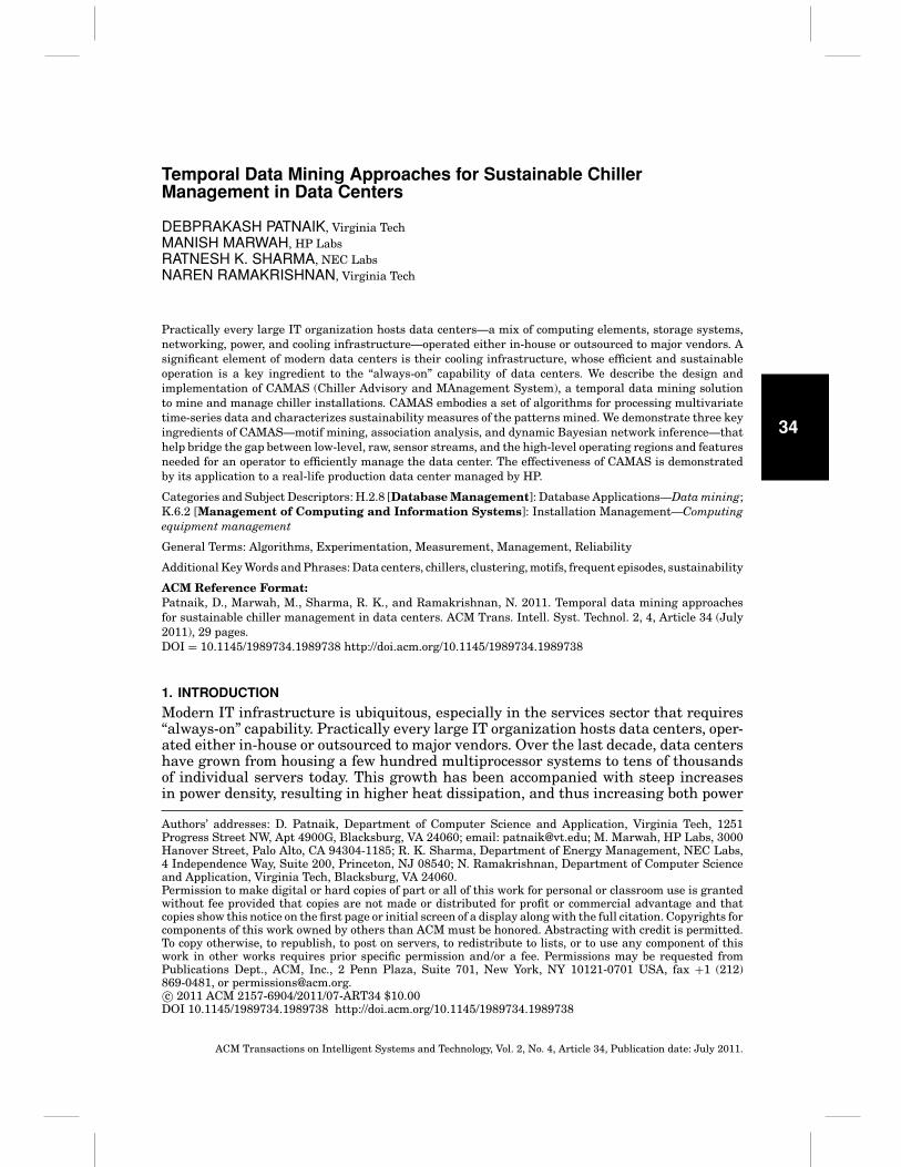
Figure 1(a) shows a data center consisting of IT equipment (servers, storage, network-ing) fitted in racks arranged as rows. A large data center could contain thousands ofracks occupying several tens of thousands of square feet of space. Also shown in thefigure are Computer Room Air Conditioning (CRAC) units that cool the exhaust hotair from the IT racks. Energy consumption in data center cooling comprises work doneto distribute the cool air and to extract heat from the hot exhaust air. A refrigeratedor chilled water cooling coil in a CRAC unit extracts the heat from the air and cools itwithin a range of 10◦C to 18◦C. The cooling infrastructure of a data center is shown inFigure 1(b).

Key elements of this infrastructure include CRAC units, plumbing and pumps forchilled water distribution, chiller units, and cooling towers. Heat dissipated from ITequipment is extracted by CRAC units and transferred to the chilled water distributionsystem. Chillers extract heat from the chilled water system and reject it to the envi-ronment through cooling towers or heat exchangers. In addition to the IT equipment,the data center cooling infrastructure can account for up to 50% of the total powerdemand [Belady 2007]. The CRAC units provide two actuators that can be controlled.The Variable Frequency Drive (VFD) controls the blower speed and the chilled watervalue regulates the amount of chilled water flowing into a unit (between 0% and 100%).These built-in flexibilities allow the units to be adjusted according to the workload de-mand in the data center. The demand is detected via temperature sensors installed onthe racks throughout a data center.

2.2. Data Center Chillers

As stated earlier, the focus of this article is on chiller units that receive warm water(at temperature, Tin) from the CRAC units, extract heat from it, and recirculate thechilled water (at temperature, Tout) back to the CRAC units.

Each chiller is composed of four basic components, namely, evaporator, multistagecentrifugal compressor, economizer, and water-cooled or air-cooled condenser. Liquidrefrigerant is distributed along the length of the evaporator to absorb enough heat fromthe water returning from the data center and circulated through the evaporator tubes tovaporize. The gaseous refrigerant is then drawn into the first stage of the compressor.Compressed gas passes from the multistage compressor into the condenser. Cooling



(b)

Fig. 1. (a) Thermal map of a data center showing racks arranged in rows and CRAC units, and (b) typicalcooling infrastructure of a data center.

tower water circulated through the condenser tubes absorbs heat from the refrigerant,causing it to condense. The liquid refrigerant then passes through an orifice plate intothe economizer. Flashed gases enter the compressor while the liquid flows into theevaporator to complete the circuit.

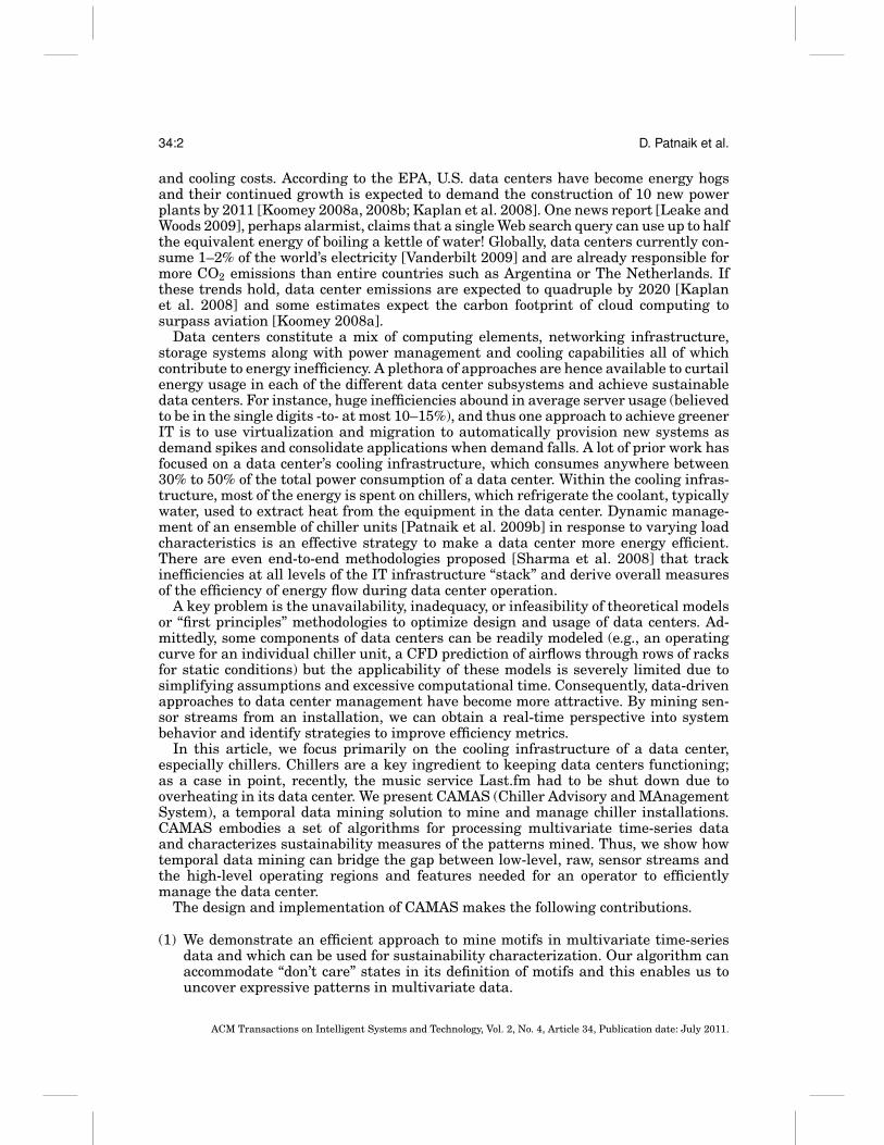
Starting and stopping a chiller is a complex, multistep process. Figure 2 shows theoperational state diagram of a typical chiller. On power-on, the chiller waits for thecompressors to start, after a prescribed delay. On startup, the chiller utilization variesto match the cooling load. Based on chiller technology, chiller compressors can throttlein discrete stages or continuously. Feedback control is used to maintain the outlettemperature, Tout, close to a user-specified set-point temperature.

We define some terms used in the context of a data center chiller unit.

—IT cooling load. This is the amount of heat that is generated (and thus needs to bedissipated) at a data center. It is approximately equivalent to the power consumedby the equipment since almost all of it is dissipated as heat. It is commonly specifiedin kilowatts (KW).



Fig. 2. Operational state diagram of a chiller unit.

—COP. The Coefficient Of Performance (COP) of a chiller unit indicates how efficientlythe unit provides cooling, and is defined as the ratio between the cooling providedand the power consumed, that is,

COPi = Li

Pi, (1)

where Li is the cooling load on the ith chiller unit and Pi is the power consumed byit. In the data center studied in this work the typical values of COP for air-cooledchillers and water-cooled chillers are 3.5 and 6.5, respectively.

—Chiller utilization. This is the percentage of the total capacity of a chiller unit thatis in use. It depends on a variety of factors, mainly, the mass flow rate of water thatpasses through a chiller and the degree of cooling provided, that is, the differencebetween the inlet and outlet temperatures (Tin − Tout). For a particular Tout, anadministrator can control the utilization at a chiller through power capping or bychanging the mass flow rate of water. The air-cooled chillers are operated in swing-mode to handle rapidly changing cooling load and their utilizations typically vary inthe range 20–80%. On the other hand the water-cooled chillers are operated at highutilization ≈80% and handle the base cooling load.

—Chiller power consumption. This is simply the power consumed by a chiller unit.Although power meters that measure aggregate power consumption of data centerinfrastructure elements are usually available, meters that measure power consumedby an individual entity or a specific group (e.g., chillers) may not always be installed.In such cases, if the capacity of the unit and average COP are known, they, togetherwith unit utilization, can be used to estimate power consumed. We have

Pi = Ui ∗ Ci

100 ∗ COPi, (2)

where Pi is the power consumed, Ui the utilization, and Ci the capacity, all pertainingto the ith chiller unit.

2.3. Ensembles of Chiller Units

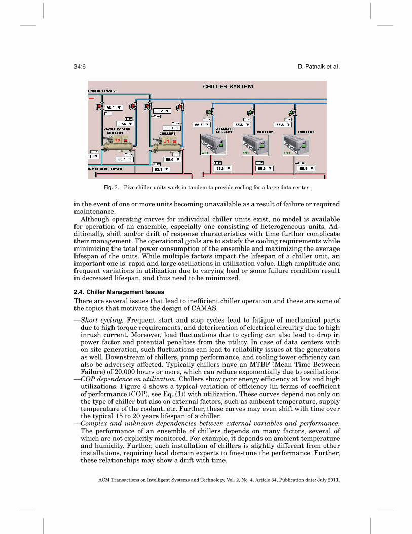
The number of chiller units required depends on the size and thermal density of adata center. While one unit may be sufficient for a small data center, several unitsoperating as an ensemble may be required to satisfy the cooling demand of a large datacenter. Figure 3 shows an ensemble of chiller units that collectively provide cooling fora data center. Out of the five units shown, three are air-cooled while the remaining twoare water-cooled. Also, to provide a highly available data center and ensure businesscontinuity, sufficient spare capacity is usually provisioned to meet the cooling demand



Fig. 3. Five chiller units work in tandem to provide cooling for a large data center.

in the event of one or more units becoming unavailable as a result of failure or requiredmaintenance.

Although operating curves for individual chiller units exist, no model is availablefor operation of an ensemble, especially one consisting of heterogeneous units. Ad-ditionally, shift and/or drift of response characteristics with time further complicatetheir management. The operational goals are to satisfy the cooling requirements whileminimizing the total power consumption of the ensemble and maximizing the averagelifespan of the units. While multiple factors impact the lifespan of a chiller unit, animportant one is: rapid and large oscillations in utilization value. High amplitude andfrequent variations in utilization due to varying load or some failure condition resultin decreased lifespan, and thus need to be minimized.

2.4. Chiller Management Issues

There are several issues that lead to inefficient chiller operation and these are some ofthe topics that motivate the design of CAMAS.

—Short cycling. Frequent start and stop cycles lead to fatigue of mechanical partsdue to high torque requirements, and deterioration of electrical circuitry due to highinrush current. Moreover, load fluctuations due to cycling can also lead to drop inpower factor and potential penalties from the utility. In case of data centers withon-site generation, such fluctuations can lead to reliability issues at the generatorsas well. Downstream of chillers, pump performance, and cooling tower efficiency canalso be adversely affected. Typically chillers have an MTBF (Mean Time BetweenFailure) of 20,000 hours or more, which can reduce exponentially due to oscillations.

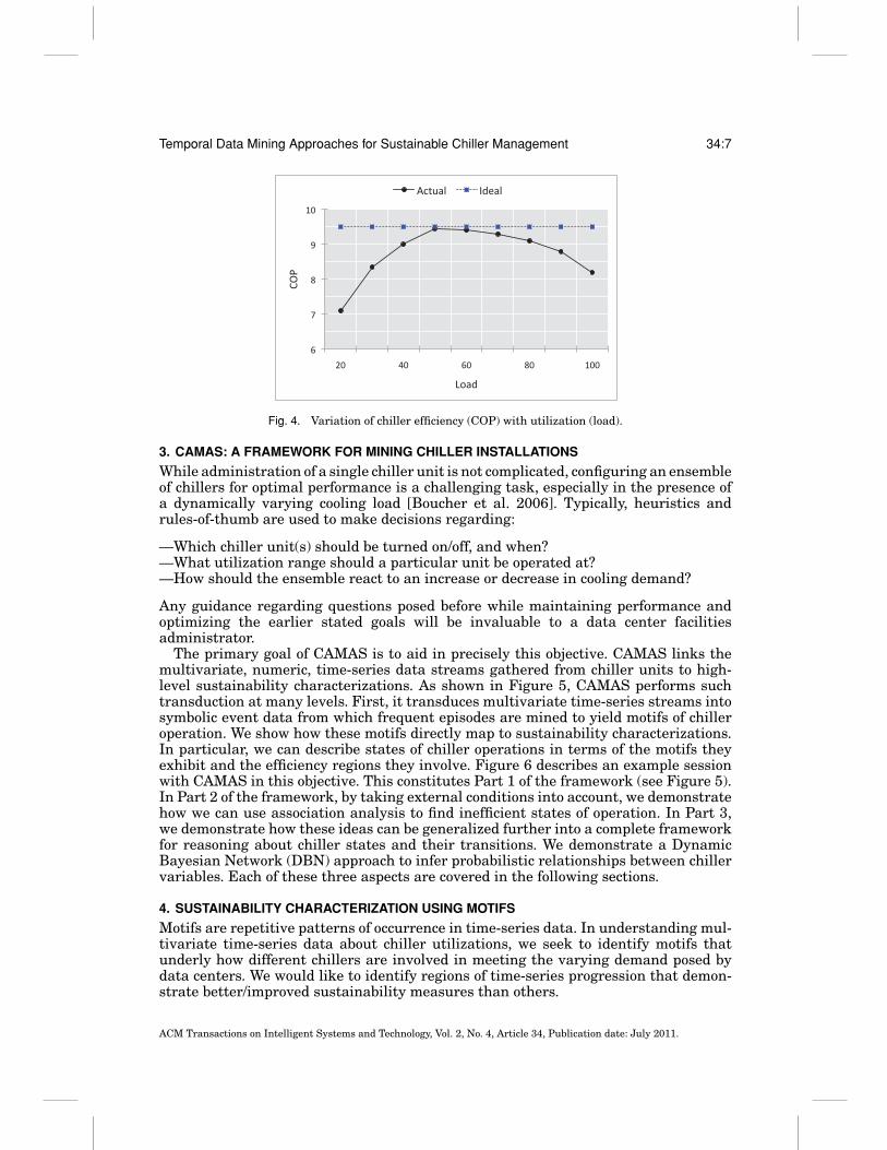
—COP dependence on utilization. Chillers show poor energy efficiency at low and highutilizations. Figure 4 shows a typical variation of efficiency (in terms of coefficientof performance (COP), see Eq. (1)) with utilization. These curves depend not only onthe type of chiller but also on external factors, such as ambient temperature, supplytemperature of the coolant, etc. Further, these curves may even shift with time overthe typical 15 to 20 years lifespan of a chiller.

—Complex and unknown dependencies between external variables and performance.The performance of an ensemble of chillers depends on many factors, several ofwhich are not explicitly monitored. For example, it depends on ambient temperatureand humidity. Further, each installation of chillers is slightly different from otherinstallations, requiring local domain experts to fine-tune the performance. Further,these relationships may show a drift with time.



Fig. 4. Variation of chiller efficiency (COP) with utilization (load).

3. CAMAS: A FRAMEWORK FOR MINING CHILLER INSTALLATIONS

While administration of a single chiller unit is not complicated, configuring an ensembleof chillers for optimal performance is a challenging task, especially in the presence ofa dynamically varying cooling load [Boucher et al. 2006]. Typically, heuristics andrules-of-thumb are used to make decisions regarding:

—Which chiller unit(s) should be turned on/off, and when?—What utilization range should a particular unit be operated at?—How should the ensemble react to an increase or decrease in cooling demand?

Any guidance regarding questions posed before while maintaining performance andoptimizing the earlier stated goals will be invaluable to a data center facilitiesadministrator.

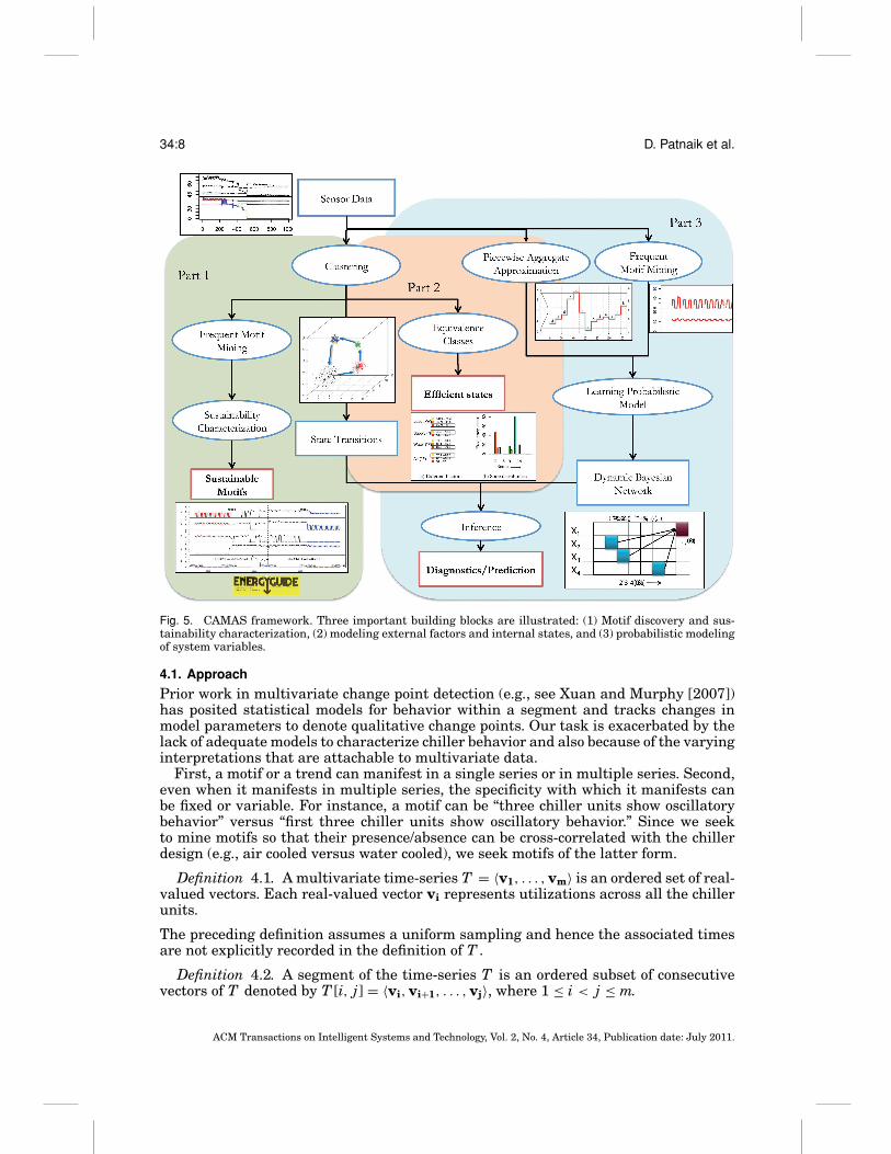
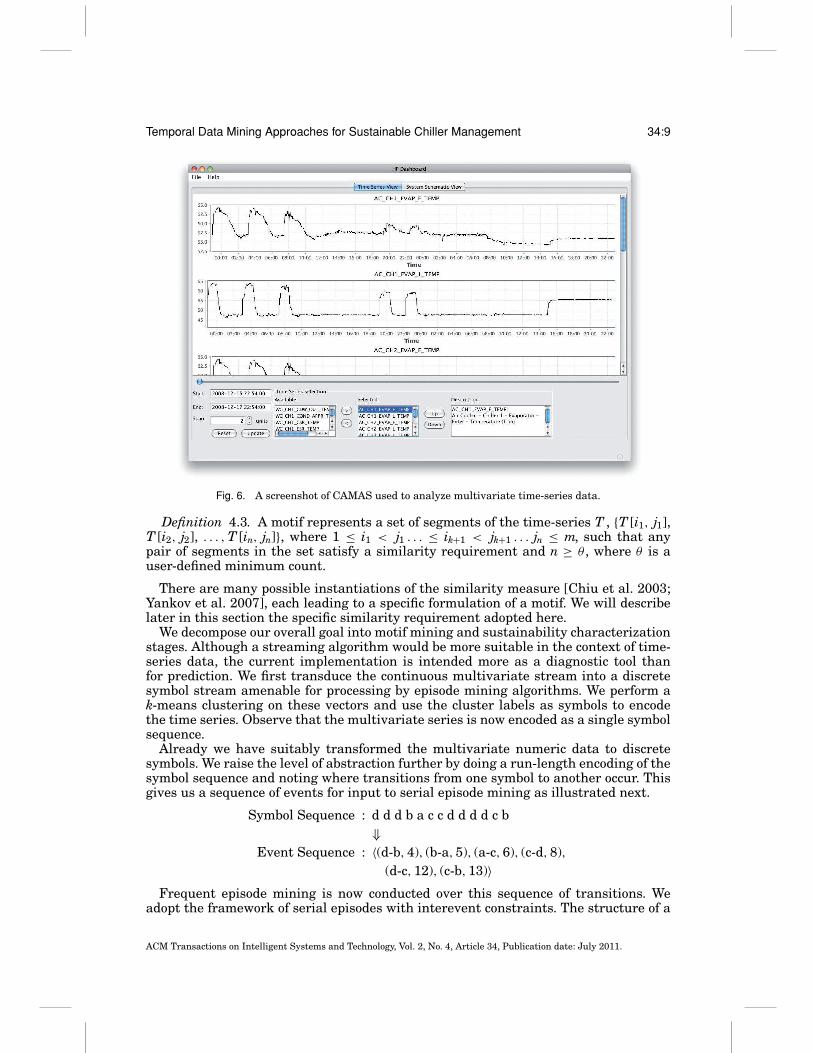
The primary goal of CAMAS is to aid in precisely this objective. CAMAS links themultivariate, numeric, time-series data streams gathered from chiller units to high-level sustainability characterizations. As shown in Figure 5, CAMAS performs suchtransduction at many levels. First, it transduces multivariate time-series streams intosymbolic event data from which frequent episodes are mined to yield motifs of chilleroperation. We show how these motifs directly map to sustainability characterizations.In particular, we can describe states of chiller operations in terms of the motifs theyexhibit and the efficiency regions they involve. Figure 6 describes an example sessionwith CAMAS in this objective. This constitutes Part 1 of the framework (see Figure 5).In Part 2 of the framework, by taking external conditions into account, we demonstratehow we can use association analysis to find inefficient states of operation. In Part 3,we demonstrate how these ideas can be generalized further into a complete frameworkfor reasoning about chiller states and their transitions. We demonstrate a DynamicBayesian Network (DBN) approach to infer probabilistic relationships between chillervariables. Each of these three aspects are covered in the following sections.

4. SUSTAINABILITY CHARACTERIZATION USING MOTIFS

Motifs are repetitive patterns of occurrence in time-series data. In understanding mul-tivariate time-series data about chiller utilizations, we seek to identify motifs thatunderly how different chillers are involved in meeting the varying demand posed bydata centers. We would like to identify regions of time-series progression that demon-strate better/improved sustainability measures than others.



Fig. 5. CAMAS framework. Three important building blocks are illustrated: (1) Motif discovery and sus-tainability characterization, (2) modeling external factors and internal states, and (3) probabilistic modelingof system variables.

4.1. Approach

Prior work in multivariate change point detection (e.g., see Xuan and Murphy [2007])has posited statistical models for behavior within a segment and tracks changes inmodel parameters to denote qualitative change points. Our task is exacerbated by thelack of adequate models to characterize chiller behavior and also because of the varyinginterpretations that are attachable to multivariate data.

First, a motif or a trend can manifest in a single series or in multiple series. Second,even when it manifests in multiple series, the specificity with which it manifests canbe fixed or variable. For instance, a motif can be “three chiller units show oscillatorybehavior” versus “first three chiller units show oscillatory behavior.” Since we seekto mine motifs so that their presence/absence can be cross-correlated with the chillerdesign (e.g., air cooled versus water cooled), we seek motifs of the latter form.

Definition 4.1. A multivariate time-series T = 〈v1, . . . , vm〉 is an ordered set of real-valued vectors. Each real-valued vector vi represents utilizations across all the chillerunits.

The preceding definition assumes a uniform sampling and hence the associated timesare not explicitly recorded in the definition of T .

Definition 4.2. A segment of the time-series T is an ordered subset of consecutivevectors of T denoted by T [i, j] = 〈vi, vi+1, . . . , vj〉, where 1 ≤ i < j ≤ m.



Fig. 6. A screenshot of CAMAS used to analyze multivariate time-series data.

Definition 4.3. A motif represents a set of segments of the time-series T , {T [i1, j1],T [i2, j2], . . . , T [in, jn]}, where 1 ≤ i1 < j1 . . . ≤ ik+1 < jk+1 . . . jn ≤ m, such that anypair of segments in the set satisfy a similarity requirement and n ≥ θ , where θ is auser-defined minimum count.

There are many possible instantiations of the similarity measure [Chiu et al. 2003;Yankov et al. 2007], each leading to a specific formulation of a motif. We will describelater in this section the specific similarity requirement adopted here.

We decompose our overall goal into motif mining and sustainability characterizationstages. Although a streaming algorithm would be more suitable in the context of time-series data, the current implementation is intended more as a diagnostic tool thanfor prediction. We first transduce the continuous multivariate stream into a discretesymbol stream amenable for processing by episode mining algorithms. We perform ak-means clustering on these vectors and use the cluster labels as symbols to encodethe time series. Observe that the multivariate series is now encoded as a single symbolsequence.

Already we have suitably transformed the multivariate numeric data to discretesymbols. We raise the level of abstraction further by doing a run-length encoding of thesymbol sequence and noting where transitions from one symbol to another occur. Thisgives us a sequence of events for input to serial episode mining as illustrated next.

Symbol Sequence : d d d b a c c d d d d c b⇓

Event Sequence : 〈(d-b, 4), (b-a, 5), (a-c, 6), (c-d, 8),(d-c, 12), (c-b, 13)〉

Frequent episode mining is now conducted over this sequence of transitions. Weadopt the framework of serial episodes with interevent constraints. The structure of a



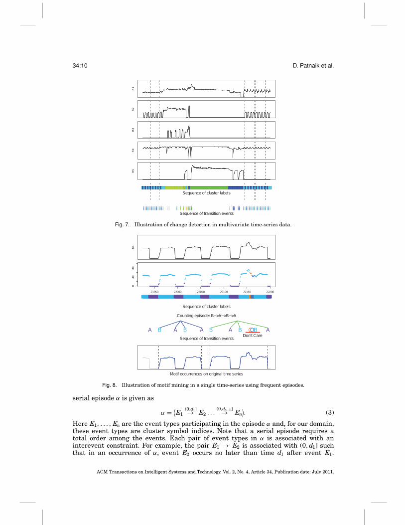
Fig. 7. Illustration of change detection in multivariate time-series data.

Fig. 8. Illustration of motif mining in a single time-series using frequent episodes.

serial episode α is given as

α = ⟨E1

(0,d1]→ E2 . . .(0,dn−1]→ En

⟩. (3)

Here E1, . . . , En are the event types participating in the episode α and, for our domain,these event types are cluster symbol indices. Note that a serial episode requires atotal order among the events. Each pair of event types in α is associated with aninterevent constraint. For example, the pair E1 → E2 is associated with (0, d1] suchthat in an occurrence of α, event E2 occurs no later than time d1 after event E1.



Referring back to our definition of a motif, we see that the similarity requirement isthus every pair of segments must have an occurrence of the same serial episode definedover transition events. A key feature of episode mining is that the event occurrencescan be interspersed with “don’t care” states and this enables us to uncover expressivepatterns in the sequential data. While other approaches exist to accommodate don’tcare states [Chiu et al. 2003], our algorithm is deterministic and guarantees findingrepeating patterns in the discrete domain with a given support threshold. However,some patterns in the raw time-series can go unnoticed due to coarse discretization.

4.2. Algorithms

The mining process follows the level-wise procedure ala Apriori, that is, candidate gen-eration followed by counting. The candidate generation scheme is based on matchingthe n − 1 size suffix of one n-node frequent episode with the n − 1 size prefix of theanother n-node frequent episode at a given level to generate candidates for the nextlevel. The time complexity of the candidate generation process is O(m2n), where n is thesize of each frequent episode in the given level, m is the number of frequent episodesin that level, since all pairs of frequent episodes need to be compared for a prefix-suffixmatch.

The algorithm for counting the set of candidates episodes is given in Algorithm 1.The count or frequency measure is based on nonoverlapped occurrences [Laxman et al.2005]. Two occurrences of an episode are said to be nonoverlapped if the events inone occurrence appear between the events in the other occurrence. This notion mostnaturally eliminates the problem of trivial matches highlighted in Patel et al. [2002]where a match is found between two slightly shifted segments of the time series.Algorithm 1 takes as input the event-sequence and a set of candidate episodes andreturns the set of frequent episodes for a given frequency threshold θ . The algorithmcounts the maximum number of nonoverlapped occurrences of each episode with theinterevent time constraint (0, T ]. This approach also allows repeated symbols or eventsin the episodes.

ALGORITHM 1: Counting occurrences of serial episodes with interevent time constraint [0, T )Input: Candidate episodes C = {α1, . . . , αm}, where αi = Eαi (1) → . . . Eαi (N) is a N-node episode,

Inter-event time constraint T and frequency threshold θ , Event sequence S = {(Ei, ti)}.Output: Frequent episodes F : α ∈ F if α.count ≥ θ1: /*Initialize*/2: waits = φ3: for all α ∈ C do4: α.count = 05: s = Array of size N, each cell initialized to -∞6: for i = 1 to|α| do7: waits[Eα(i)].append(α, s, i)8: for all (Ek, tk) ∈ S do9: for all (α, s, i) ∈ waits[Ek] do10: if (i = 1) or (tk − s[i − 1] ≤ T ) then11: /*First event or Satisfies the time constraint*/12: if (i = |α|) then13: α.count = α.count + 114: Reinitialize all elements of s to −∞15: else16: s[i] = tk17: Output F = {α : α ∈ C such that α.count ≥ θ}



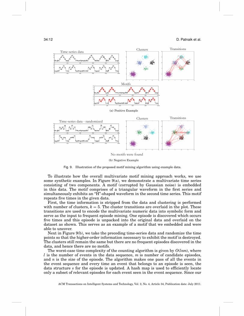
Fig. 9. Illustration of the proposed motif mining algorithm using example data.

To illustrate how the overall multivariate motif mining approach works, we usesome synthetic examples. In Figure 9(a), we demonstrate a multivariate time seriesconsisting of two components. A motif (corrupted by Gaussian noise) is embeddedin this data. The motif comprises of a triangular waveform in the first series andsimultaneously exhibits an “H”-shaped waveform in the second time series. This motifrepeats five times in the given data.

First, the time information is stripped from the data and clustering is performedwith number of clusters, k = 5. The cluster transitions are overlaid in the plot. Thesetransitions are used to encode the multivariate numeric data into symbolic form andserve as the input to frequent episode mining. One episode is discovered which occursfive times and this episode is unpacked into the original data and overlaid on thedataset as shown. This serves as an example of a motif that we embedded and wereable to uncover.

Next in Figure 9(b), we take the preceding time-series data and randomize the timepoints so that the higher-order information necessary to exhibit the motif is destroyed.The clusters still remain the same but there are no frequent episodes discovered in thedata, and hence there are no motifs.

The worst-case time complexity of the counting algorithm is given by O(lnm), wherel is the number of events in the data sequence, m is number of candidate episodes,and n is the size of the episode. The algorithm makes one pass of all the events inthe event sequence and every time an event that belongs to an episode is seen, thedata structure s for the episode is updated. A hash map is used to efficiently locateonly a subset of relevant episodes for each event seen in the event sequence. Since our



method allows repeated symbols, in the case of such episodes the same event can updates structure at most n times. Therefore if the level-wise growth of candidates is suffi-ciently arrested by a suitably chosen threshold, the algorithm scales linearly with datasize.

Recall here that the events in mined frequent episodes correspond to transitions fromone symbol to another. Our hypothesis here is that if motif occurrences are matched attransitions under an intertransition gap constraint, then the corresponding time-seriessubsequences will match under a suitable distance metric. In addition the episode min-ing framework allows for robustness to noise and scaling. The distance metric underwhich such motifs can be shown to be similar needs further investigation. Nonethelessthis technique is found to be very effective in unearthing similar time-series subse-quences in real datasets.

4.3. Sustainability Characterization

It is difficult (and subjective) to compare two motifs in terms of their sustainabilityimpact by inspecting them visually. Therefore, it is necessary to quantify the sustain-ability of all motifs by computing a sustainability metric for them. This would enablequantitative comparisons between motifs; their categorization as “good” or “bad” fromthe sustainability metric point-of-view; and, furthermore, this information could beused to provide guidance to an administrator or a management system regarding themost “sustainable” configurations of the chiller ensemble under a particular load. Thereare several sustainability metrics, such as power consumed, carbon footprint, and ex-ergy loss [Shah et al. 2008], where exergy is defined as the energy that is available to beused. Note that typically optimizing a sustainability metric, such as power consumed,also minimizes the total cost of operation.

In this article, we estimate two sustainability metrics for each motif: (1) the averageCOP of the motif; and, (2) a metric reflecting the frequency and amplitude of oscillationsin utilization values. The average COP is calculated using Eq. (1), where the loadduring motif i, averaged over all its occurrences, is used as Li and the averaged powerconsumption of the motif as Pi. The power is estimated using Eq. (2) with an averagedconstant COP of 3.5 for the air-cooled and 6 for the water-cooled chillers. The COP ofa motif quantifies the cooling effectiveness of the ensemble during that motif. In orderto estimate the frequency of oscillations of a motif, we compute the number of mean-crossings, that is, the number of times the utilization crosses the mean value. This isvery similar to number of zero-crossings that is commonly used in speech processingfor estimation of frequency. This, together with standard deviation of a motif, allowsoscillatory behavior to be compared.

4.4. Results

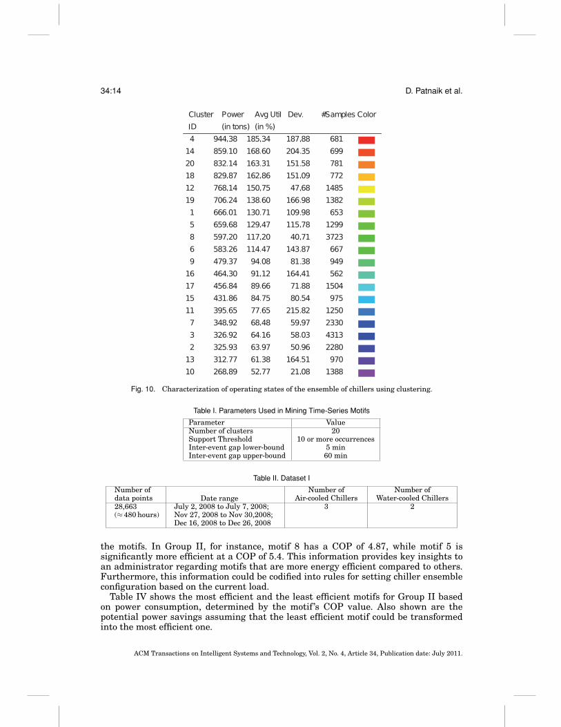
We applied our motif mining methodology to chiller data obtained from a large HPproduction data center covering 70,000 square feet with 2000 racks of IT equipment.Its cooling demand is met by an ensemble of five chiller units. The ensemble consists oftwo types of chillers: three are air-cooled and the remaining two are water-cooled. Thedata characteristics are given in Table II. We mined 20 clusters from this data, with aview toward identifying well-separated clusters.

4.4.1. Motifs. All the parameters using in mining motifs in multivariate time-seriesdata is shown in Table I. In all, 22 motifs were discovered in the chiller utilization datawhose qualitative properties are summarized in Table V (more on this later). Froma quantitative point of view these motifs can be clustered into groups based on load.One such group (Group II) is depicted in Table III with other quantitative measures.Although each group has very similar load levels, the COP within a group varies with



Fig. 10. Characterization of operating states of the ensemble of chillers using clustering.

Table I. Parameters Used in Mining Time-Series Motifs

Parameter ValueNumber of clusters 20Support Threshold 10 or more occurrencesInter-event gap lower-bound 5 minInter-event gap upper-bound 60 min

Table II. Dataset I

Number ofdata points Date range

Number ofAir-cooled Chillers

Number ofWater-cooled Chillers

28,663(≈ 480 hours)

July 2, 2008 to July 7, 2008;Nov 27, 2008 to Nov 30,2008;Dec 16, 2008 to Dec 26, 2008

3 2

the motifs. In Group II, for instance, motif 8 has a COP of 4.87, while motif 5 issignificantly more efficient at a COP of 5.4. This information provides key insights toan administrator regarding motifs that are more energy efficient compared to others.Furthermore, this information could be codified into rules for setting chiller ensembleconfiguration based on the current load.

Table IV shows the most efficient and the least efficient motifs for Group II basedon power consumption, determined by the motif ’s COP value. Also shown are thepotential power savings assuming that the least efficient motif could be transformedinto the most efficient one.



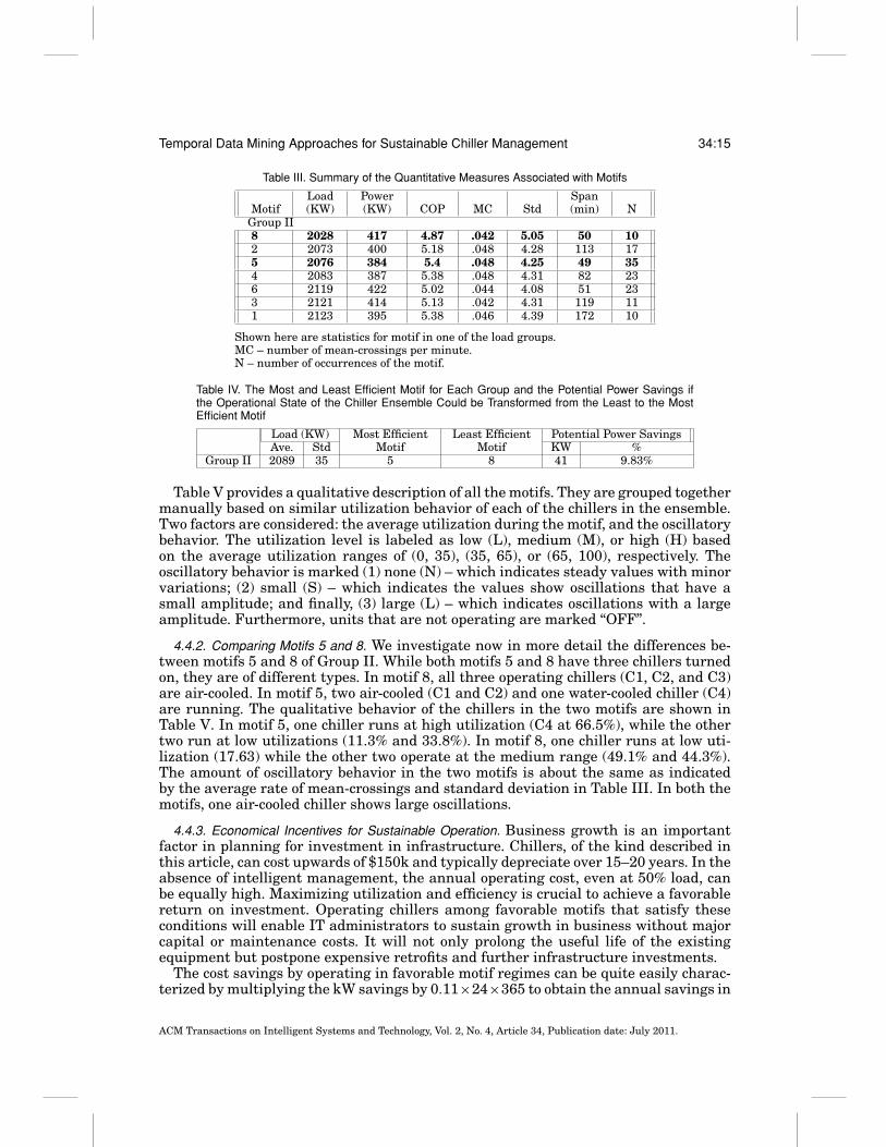
Table III. Summary of the Quantitative Measures Associated with Motifs

Load Power SpanMotif (KW) (KW) COP MC Std (min) N

Group II8 2028 417 4.87 .042 5.05 50 102 2073 400 5.18 .048 4.28 113 175 2076 384 5.4 .048 4.25 49 354 2083 387 5.38 .048 4.31 82 236 2119 422 5.02 .044 4.08 51 233 2121 414 5.13 .042 4.31 119 111 2123 395 5.38 .046 4.39 172 10

Shown here are statistics for motif in one of the load groups.MC – number of mean-crossings per minute.N – number of occurrences of the motif.

Table IV. The Most and Least Efficient Motif for Each Group and the Potential Power Savings ifthe Operational State of the Chiller Ensemble Could be Transformed from the Least to the MostEfficient Motif

Load (KW) Most Efficient Least Efficient Potential Power SavingsAve. Std Motif Motif KW %

Group II 2089 35 5 8 41 9.83%

Table V provides a qualitative description of all the motifs. They are grouped togethermanually based on similar utilization behavior of each of the chillers in the ensemble.Two factors are considered: the average utilization during the motif, and the oscillatorybehavior. The utilization level is labeled as low (L), medium (M), or high (H) basedon the average utilization ranges of (0, 35), (35, 65), or (65, 100), respectively. Theoscillatory behavior is marked (1) none (N) – which indicates steady values with minorvariations; (2) small (S) – which indicates the values show oscillations that have asmall amplitude; and finally, (3) large (L) – which indicates oscillations with a largeamplitude. Furthermore, units that are not operating are marked “OFF”.

4.4.2. Comparing Motifs 5 and 8. We investigate now in more detail the differences be-tween motifs 5 and 8 of Group II. While both motifs 5 and 8 have three chillers turnedon, they are of different types. In motif 8, all three operating chillers (C1, C2, and C3)are air-cooled. In motif 5, two air-cooled (C1 and C2) and one water-cooled chiller (C4)are running. The qualitative behavior of the chillers in the two motifs are shown inTable V. In motif 5, one chiller runs at high utilization (C4 at 66.5%), while the othertwo run at low utilizations (11.3% and 33.8%). In motif 8, one chiller runs at low uti-lization (17.63) while the other two operate at the medium range (49.1% and 44.3%).The amount of oscillatory behavior in the two motifs is about the same as indicatedby the average rate of mean-crossings and standard deviation in Table III. In both themotifs, one air-cooled chiller shows large oscillations.

4.4.3. Economical Incentives for Sustainable Operation. Business growth is an importantfactor in planning for investment in infrastructure. Chillers, of the kind described inthis article, can cost upwards of $150k and typically depreciate over 15–20 years. In theabsence of intelligent management, the annual operating cost, even at 50% load, canbe equally high. Maximizing utilization and efficiency is crucial to achieve a favorablereturn on investment. Operating chillers among favorable motifs that satisfy theseconditions will enable IT administrators to sustain growth in business without majorcapital or maintenance costs. It will not only prolong the useful life of the existingequipment but postpone expensive retrofits and further infrastructure investments.

The cost savings by operating in favorable motif regimes can be quite easily charac-terized by multiplying the kW savings by 0.11×24×365 to obtain the annual savings in



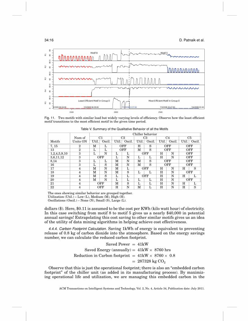
Fig. 11. Two motifs with similar load but widely varying levels of efficiency. Observe how the least efficientmotif transitions to the most efficient motif in the given time period.

Table V. Summary of the Qualitative Behavior of all the Motifs

Chiller behaviorNum of C1 C2 C3 C4 C5

Motifs Units ON Util. Oscil. Util. Oscil. Util. Oscil. Util. Oscil. Util. Oscil.7, 15 2 M L OFF H S OFF OFF13 2 L L OFF M S OFF OFF1,2,4,5,9,10 3 L N L L OFF H N OFF3,6,11,12 3 OFF L N L L H N OFF8,14 3 L L M N M S OFF OFF16 3 L S M N M S OFF OFF17 4 M N M L OFF H N H S18 4 M N M S L L H N OFF19 4 M S L L OFF H N H L20 4 M N L L L L H N OFF21 4 OFF M S L L H N H L22 4 OFF H N M L H N H S

The ones showing similar behavior are grouped together.Utilization (Util.) – Low (L), Medium (M), High (H).Oscillations (Oscil.) – None (N), Small (S), Large (L).

dollars ($). Here, $0.11 is assumed to be the cost per KWh (kilo watt hour) of electricity.In this case switching from motif 8 to motif 5 gives us a nearly $40,000 in potentialannual savings! Extrapolating this cost saving to other similar motifs gives us an ideaof the utility of data mining algorithms in helping achieve cost effectiveness.

4.4.4. Carbon Footprint Calculation. Saving 1kWh of energy is equivalent to preventingrelease of 0.8 kg of carbon dioxide into the atmosphere. Based on the energy savingsnumber, we can calculate the reduced carbon footprint.

Saved Power = 41kWSaved Energy (annually) = 41kW × 8760 hrs

Reduction in Carbon footprint = 41kW × 8760 × 0.8= 287328 kg CO2

Observe that this is just the operational footprint; there is also an “embedded carbonfootprint” of the chiller unit (as added in its manufacturing process). By maximiz-ing operational life and utilization, we are managing this embedded carbon in the



equipment as well. In other words, we are limiting the increase in embedded carbon inthe environment while delivering the cooling required.

5. MODELING THE INFLUENCE OF EXTERNAL VARIABLES

While motifs are very useful in assessing repetitive patterns of occurrence, they con-stitute only a relative minority of the state space that the chiller ensemble operates in.Another interesting goal is to characterize the regions of state space occupied by thechiller ensemble and correlate them to the external conditions that the data center,and in particular, the chiller ensemble is subjected to. Once again, we focus on theutilization vectors of the same chiller system. But after a recent upgrade, the installa-tion now has seven chillers instead of five as described earlier: five air-cooled and twowater-cooled. We demonstrate the use of association analysis techniques to identify keyconditions that underlie sources of inefficiency.

5.1. Approach

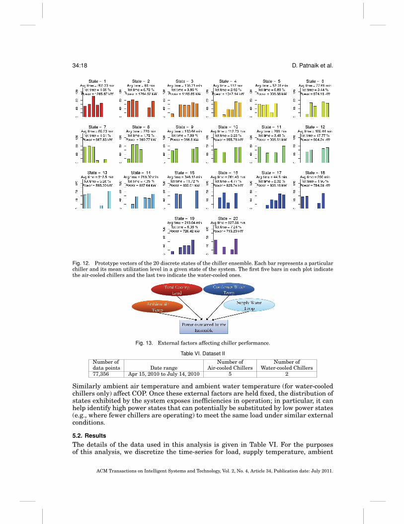
We discretize the utilization state space of chillers by clustering using seed prototypevectors. The seed prototypes are obtained by combining low, medium, and high utiliza-tion values for individual chiller units to obtain a total of 37 = 2187 prototype utilizationvectors. These prototypes are used to seed clusters for a k-means algorithm and clustersthat are assigned zero members are removed from the analysis. The resulting clustersare still too numerous for human consumption; consequently, we applied hierarchicalclustering with distance between pairs of clusters as the average distance between allpairs of points across the two clusters. The agglomerative process of merging clusterswas stopped at a level where there was sufficient separation between the clusters be-ing merged. This ensures that the states represent qualitatively distinct regions. Theprototypes for the final states are shown in Figure 12. Each state is annotated with thepercentage fraction of total time spent by the system in that state, the average timespent there before moving into a different state, and the average power consumed. Thestates are colored using the rainbow palette based on the power consumed in a state,red being the highest power consuming state and blue the lowest power state.

As a preliminary analysis, we can organize the states from Figure 12 in many differ-ent ways and assess their characteristics. For example, we can group the states basedon power consumption and investigate the fraction of time that is spent in, say, highpower states. We can assess the states by asking where the system spends most of itstime and determine the profile of these states in terms of the different chillers. This canbe used to validate if the load balancing objectives of the system are being met. Finally,we can also investigate which chillers are on/off in different states. In states 1, 5, and 8none of the water cooled chillers is running. This is unusual for this installation sincethe scheduling policy mandates the use of at least one water-cooled chiller at all timesto handle the base cooling load.

Given the same external conditions, the chiller ensemble is expected to exhibit similarpower consumption characteristics. For example, for a given cooling load the chillersystem should ideally consume the same amount of power. In practice, the system maynot be able to operate in the most optimal mode to meet the required load under givenexternal conditions. In CAMAS, we analyze the distribution of states observed undergiven external conditions and investigate its characteristics.

The external conditions known to influence the operations of chiller are cooling load,supply water temperature, ambient air temperature, and ambient water temperature.The cooling load is the total cooling requirement of the data center and office spaces thatare served by the chiller ensemble. The supply water temperature is the temperatureat which chiller water is supplied to the air-conditioning units. The set point of thesupply water temperature impacts the coefficient of performance (COP) of the chillers.



Fig. 12. Prototype vectors of the 20 discrete states of the chiller ensemble. Each bar represents a particularchiller and its mean utilization level in a given state of the system. The first five bars in each plot indicatethe air-cooled chillers and the last two indicate the water-cooled ones.

Fig. 13. External factors affecting chiller performance.

Table VI. Dataset II

Number of Number of Number ofdata points Date range Air-cooled Chillers Water-cooled Chillers77,356 Apr 15, 2010 to July 14, 2010 5 2

Similarly ambient air temperature and ambient water temperature (for water-cooledchillers only) affect COP. Once these external factors are held fixed, the distribution ofstates exhibited by the system exposes inefficiencies in operation; in particular, it canhelp identify high power states that can potentially be substituted by low power states(e.g., where fewer chillers are operating) to meet the same load under similar externalconditions.

5.2. Results

The details of the data used in this analysis is given in Table VI. For the purposesof this analysis, we discretize the time-series for load, supply temperature, ambient



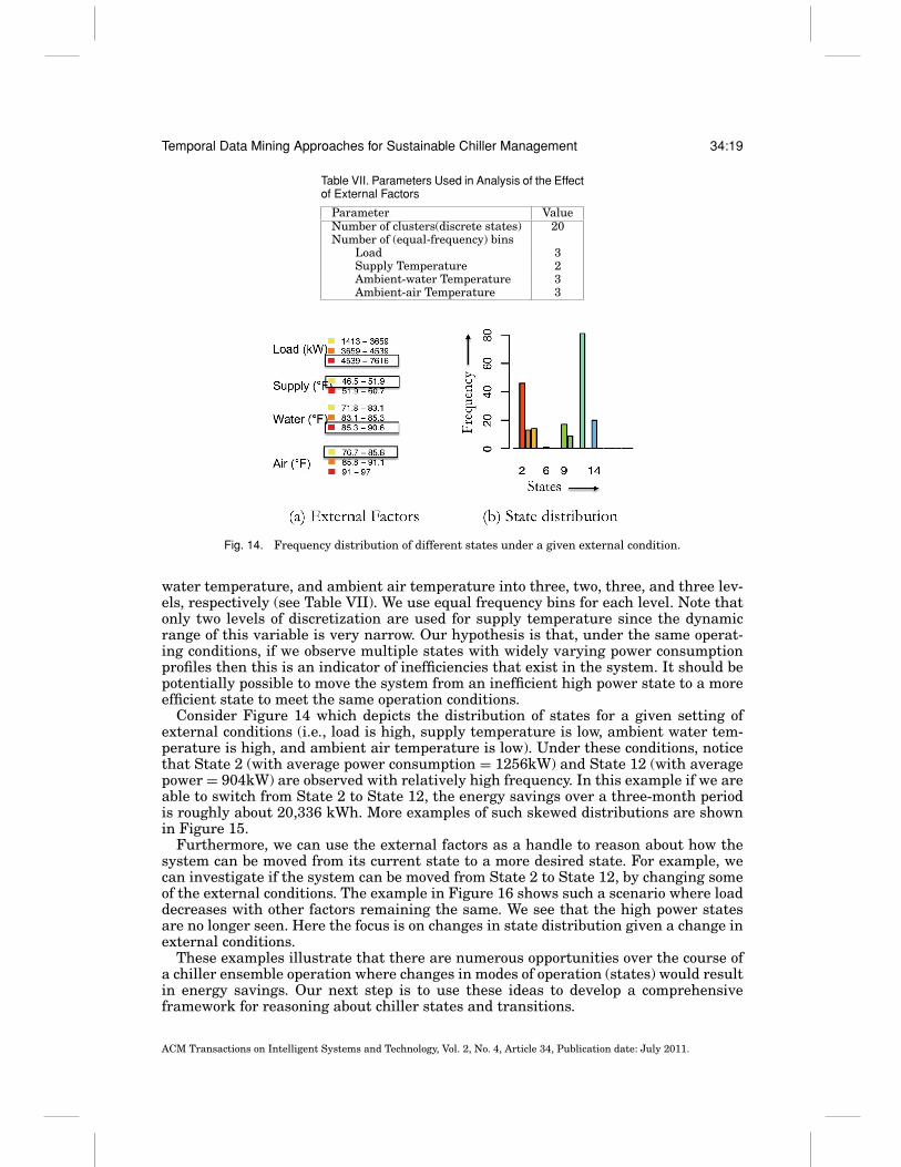
Table VII. Parameters Used in Analysis of the Effectof External Factors

Parameter ValueNumber of clusters(discrete states) 20Number of (equal-frequency) bins

Load 3Supply Temperature 2Ambient-water Temperature 3Ambient-air Temperature 3

Fig. 14. Frequency distribution of different states under a given external condition.

water temperature, and ambient air temperature into three, two, three, and three lev-els, respectively (see Table VII). We use equal frequency bins for each level. Note thatonly two levels of discretization are used for supply temperature since the dynamicrange of this variable is very narrow. Our hypothesis is that, under the same operat-ing conditions, if we observe multiple states with widely varying power consumptionprofiles then this is an indicator of inefficiencies that exist in the system. It should bepotentially possible to move the system from an inefficient high power state to a moreefficient state to meet the same operation conditions.

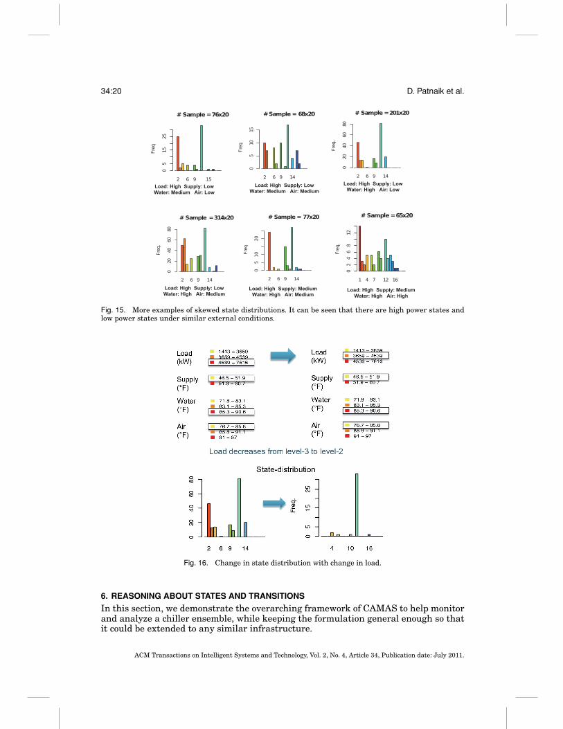
Consider Figure 14 which depicts the distribution of states for a given setting ofexternal conditions (i.e., load is high, supply temperature is low, ambient water tem-perature is high, and ambient air temperature is low). Under these conditions, noticethat State 2 (with average power consumption = 1256kW) and State 12 (with averagepower = 904kW) are observed with relatively high frequency. In this example if we areable to switch from State 2 to State 12, the energy savings over a three-month periodis roughly about 20,336 kWh. More examples of such skewed distributions are shownin Figure 15.

Furthermore, we can use the external factors as a handle to reason about how thesystem can be moved from its current state to a more desired state. For example, wecan investigate if the system can be moved from State 2 to State 12, by changing someof the external conditions. The example in Figure 16 shows such a scenario where loaddecreases with other factors remaining the same. We see that the high power statesare no longer seen. Here the focus is on changes in state distribution given a change inexternal conditions.

These examples illustrate that there are numerous opportunities over the course ofa chiller ensemble operation where changes in modes of operation (states) would resultin energy savings. Our next step is to use these ideas to develop a comprehensiveframework for reasoning about chiller states and transitions.



Fig. 15. More examples of skewed state distributions. It can be seen that there are high power states andlow power states under similar external conditions.

Fig. 16. Change in state distribution with change in load.

6. REASONING ABOUT STATES AND TRANSITIONS

In this section, we demonstrate the overarching framework of CAMAS to help monitorand analyze a chiller ensemble, while keeping the formulation general enough so thatit could be extended to any similar infrastructure.



6.1. Approach

As shown in Figure 5, data reduction is performed in a few different ways. The rawtime-series data is compressed using piece-wise aggregate approximation followingdiscretization using equal frequency bins. This helps capture the average dynamics ofthe variables. A higher-order aspect of the time series involves repeating or oscillatorybehavior. This is inferred by mining frequently repeating motifs or patterns in thetime series, as described in Section 4. This information is integrated with the averagebehavior by recording the windows in which a time series exhibits motif patterns.Finally, it is also pertinent to mine relationships involving “control” actions that weretaken during the operation of the chiller units. In this article, we focus on ON/OFFactions.

A graphical model in the form of a Dynamic Bayesian Network (DBN) is learnt fromthe preceding data. This model captures the dependencies between the variables in thesystem over different time lags. Here, we focus on the target variable of utilization andseek to identify suitable parents for modeling in the DBN. Unlike classical methods tolearn BNs [Friedman et al. 1999], we demonstrate a powerful approach to learn DBNsby creating bridges to the frequent episode mining literature [Patnaik et al. 2009a]. Toapply the learned DBN, we define states of the system by clustering together the com-bined utilization of the chiller units. This allows the operation of the chiller ensembleto be represented as a sequence of state transitions. We now use the dependencies and(conditional) independency relationships found in learning the graphical model to findthe most probable explanation behind the state transitions. This framework can thenbe applied for activities like data center diagnostics, performance improvement, loadbalancing, and preventive maintenance.

As is well known, a Bayesian Network (BN) is a graphical model denoted byB = (G, P) where G is a Directed Acyclic Graph (DAG) and P is a set of conditionalprobability distributions. The graph G = (V, E) consists of a set of nodes V represent-ing the random variables {X1, . . . , XN} in the system and a set of directed edges E. Eachdirected edge in E, denoted by i → j, indicates that random variable Xi is a parent ofrandom variable Xj . The conditional probabilities in P are used to capture statisticaldependence relationships between child nodes and parent nodes. In particular, given arandom variable Xi in the graph, we denote by par(Xi) the set of random variables thatare parents of Xi . The statistical dependence between Xi and its parent nodes par(Xi)is captured by the conditional probabilities P(Xi|par(Xi).

To model a discrete-time random process X(t), t = 1, . . . , T ; X(t) = [X1(t)X2(t)· · · XN(t)] as studied here, we use the more expressive formalism of dynamic Bayesiannetworks. In particular, we focus on time-bounded causal networks, where for a givenw > 0, the nodes in par(Xi(t)), parents for the node, Xi(t), belong to a w-length historywindow, [t − w, t). Note that parent nodes cannot belong to the current time slice t forXi(t).

This assumption limits the range-of-influence of a random variable, Xk(t), to variableswithin w time slices of t and also indicates that the random variables Xi(t) and Xj(t) areconditionally independent given their corresponding parent sets in the history window.Further, we also assume that the underlying data generation model is stationary, sothat joint statistics can be estimated using contingency tables.

The learning of network structures involves learning the parent set, par(Xi(t)), foreach Xi(t), i = 1, . . . , N. In this work we assume that there are no spurious indepen-dencies in the data, that is, if a random variable Xj(t − τ ) is a parent of Xi(t), then themutual information I(Xi(t); Xj(t − τ )|S) conditioned on a subset S ⊆ par(X) is alwaysgreater than zero. Moreover time-bounded causality enables us to learn the parents ofeach node Xi(t) independent of any other node in the same time slice. We use a greedyapproach to learn the parent set of each node Xi(t). And proceed by adding a node which



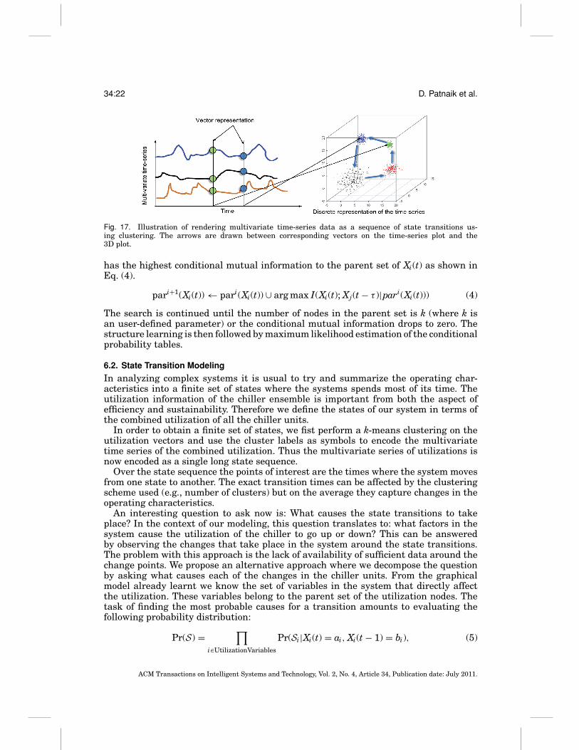
Fig. 17. Illustration of rendering multivariate time-series data as a sequence of state transitions us-ing clustering. The arrows are drawn between corresponding vectors on the time-series plot and the3D plot.

has the highest conditional mutual information to the parent set of Xi(t) as shown inEq. (4).

pari+1(Xi(t)) ← pari(Xi(t)) ∪ arg max I(Xi(t); Xj(t − τ )|pari(Xi(t))) (4)

The search is continued until the number of nodes in the parent set is k (where k isan user-defined parameter) or the conditional mutual information drops to zero. Thestructure learning is then followed by maximum likelihood estimation of the conditionalprobability tables.

6.2. State Transition Modeling

In analyzing complex systems it is usual to try and summarize the operating char-acteristics into a finite set of states where the systems spends most of its time. Theutilization information of the chiller ensemble is important from both the aspect ofefficiency and sustainability. Therefore we define the states of our system in terms ofthe combined utilization of all the chiller units.

In order to obtain a finite set of states, we fist perform a k-means clustering on theutilization vectors and use the cluster labels as symbols to encode the multivariatetime series of the combined utilization. Thus the multivariate series of utilizations isnow encoded as a single long state sequence.

Over the state sequence the points of interest are the times where the system movesfrom one state to another. The exact transition times can be affected by the clusteringscheme used (e.g., number of clusters) but on the average they capture changes in theoperating characteristics.

An interesting question to ask now is: What causes the state transitions to takeplace? In the context of our modeling, this question translates to: what factors in thesystem cause the utilization of the chiller to go up or down? This can be answeredby observing the changes that take place in the system around the state transitions.The problem with this approach is the lack of availability of sufficient data around thechange points. We propose an alternative approach where we decompose the questionby asking what causes each of the changes in the chiller units. From the graphicalmodel already learnt we know the set of variables in the system that directly affectthe utilization. These variables belong to the parent set of the utilization nodes. Thetask of finding the most probable causes for a transition amounts to evaluating thefollowing probability distribution:

Pr(S) =∏

i∈UtilizationVariables

Pr(Si|Xi(t) = ai, Xi(t − 1) = bi), (5)



Table VIII. Dataset III

Number of Number of Number ofdata points Date range Air-cooled Chillers Water-cooled Chillers28,289 Oct 21, 2009 to Nov 13, 2009 3 2(≈ 576 hrs)

Table IX. Parameters Used in State Transition Modeling

Parameter ValueNumber of clusters k (discrete states) 10Window size (for piece-wise avg. aggregation) 15 minNumber of history windows (used in DBN learning) 5

Table X. A Few Important System Variables in the Chiller Ensemble Data

System Variable DescriptionAC CH(i) EVAP E TEMP Temperature of water entering air-cooled chiller iMAIN HEADER TEMP 1 F Water temperature at distribution headerWC CH(i) IN TEMP Temperature of water entering water-cooled chiller iWC CH(i) OUT TEMP Temperature of water leaving water-cooled chiller iAC CH(i) RLA Percentage utilization of air-cooled chiller iWC CH(i) RLA Percentage utilization of water-cooled chiller i

where Si = par(Xi(t)) \ Xi(t − 1) and S = ∪Si. The most likely values that S takes canbe considered the best explanation of the transition. Here t is the time at which a statetransition occurs, ai, bi are the discrete values the utilization variable takes before andafter the state transitions. These can be approximated by the cluster centers of eachcluster used to define a state.

6.3. Results

We applied our methods to chiller data obtained from a the same data center describedin Section 4.4. All the parameters used in state transition modeling using DBNs arelisted in Table IX.

During the period from October 21, 2009 to November 13, 2009 the cooling demandof the data center was met by an ensemble of five chiller units (see Table VIII). Theensemble consists of two types of chillers: three air-cooled and the remaining two water-cooled. The data collected over this period totaled to over 576 hours of data consistingof over 47 variables.

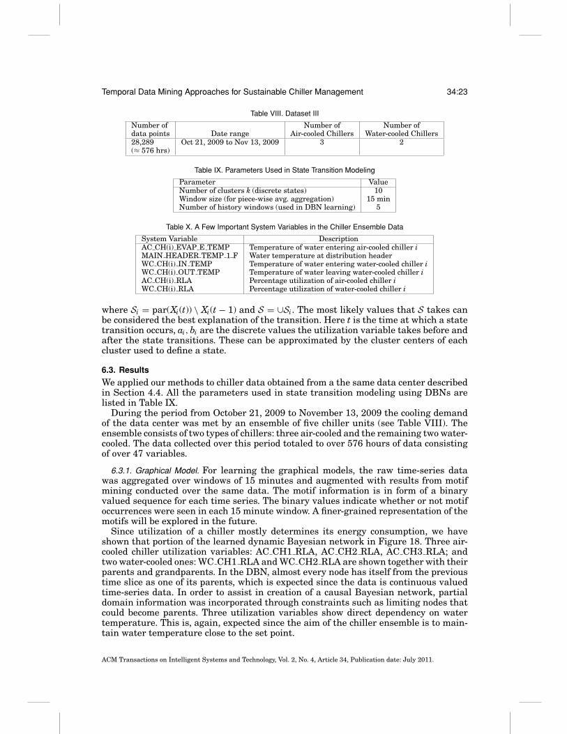
6.3.1. Graphical Model. For learning the graphical models, the raw time-series datawas aggregated over windows of 15 minutes and augmented with results from motifmining conducted over the same data. The motif information is in form of a binaryvalued sequence for each time series. The binary values indicate whether or not motifoccurrences were seen in each 15 minute window. A finer-grained representation of themotifs will be explored in the future.

Since utilization of a chiller mostly determines its energy consumption, we haveshown that portion of the learned dynamic Bayesian network in Figure 18. Three air-cooled chiller utilization variables: AC CH1 RLA, AC CH2 RLA, AC CH3 RLA; andtwo water-cooled ones: WC CH1 RLA and WC CH2 RLA are shown together with theirparents and grandparents. In the DBN, almost every node has itself from the previoustime slice as one of its parents, which is expected since the data is continuous valuedtime-series data. In order to assist in creation of a causal Bayesian network, partialdomain information was incorporated through constraints such as limiting nodes thatcould become parents. Three utilization variables show direct dependency on watertemperature. This is, again, expected since the aim of the chiller ensemble is to main-tain water temperature close to the set point.



Fig. 18. Graphical model learned from the discretized time-series data. Shown are the parent nodes for onlythe utilization variables of the five chiller units.

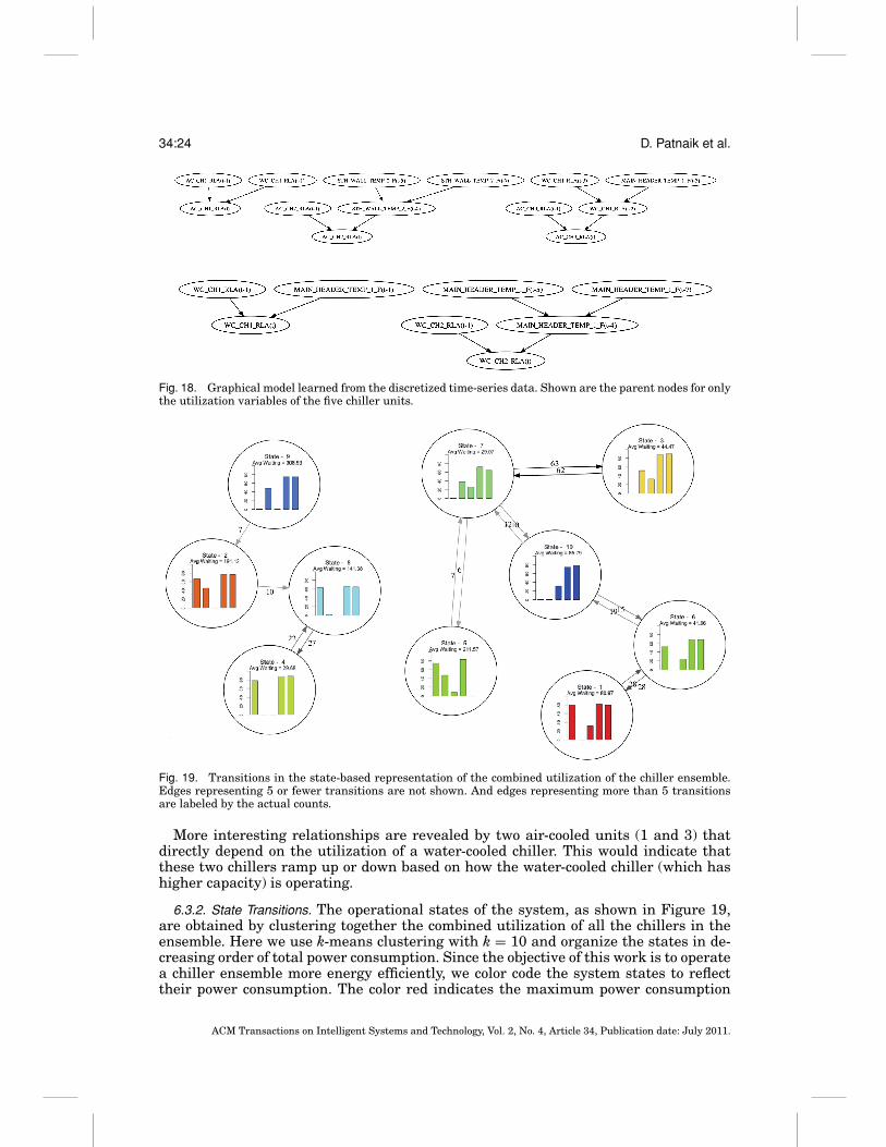
Fig. 19. Transitions in the state-based representation of the combined utilization of the chiller ensemble.Edges representing 5 or fewer transitions are not shown. And edges representing more than 5 transitionsare labeled by the actual counts.

More interesting relationships are revealed by two air-cooled units (1 and 3) thatdirectly depend on the utilization of a water-cooled chiller. This would indicate thatthese two chillers ramp up or down based on how the water-cooled chiller (which hashigher capacity) is operating.

6.3.2. State Transitions. The operational states of the system, as shown in Figure 19,are obtained by clustering together the combined utilization of all the chillers in theensemble. Here we use k-means clustering with k = 10 and organize the states in de-creasing order of total power consumption. Since the objective of this work is to operatea chiller ensemble more energy efficiently, we color code the system states to reflecttheir power consumption. The color red indicates the maximum power consumption



Table XI. List of Most Likely Value Assignments of the Parent-Set of NodeAC CH1 RLA i.e. Utilization of Air-Cooled Chiller 1

par(Xi(t)) Delay Value Pr(par(Xi(t))|Xi(t), Xi(t − 1))WC CH1 RLA 1 (75.37, 77.38] 0.27WC CH1 RLA 1 (72.36, 75.37] 0.18WC CH1 RLA 1 (77.38, 79.71] 0.18

(about 3298 KW) while the color blue indicates the least consumption (2148 KW). Alsoshown, for each state, are the average utilization values of the five chillers as a his-togram with first three (starting from the left) being air-cooled ones and the last twobeing water-cooled units. The time spent by the system in each state is also listed(maximum in state 9, while least in state). The arrows show the transitions betweenstates, with the gray-scale indicating the frequency of the transition (darkest implyingmost often).

The system states are mainly characterized by the number and kind of chiller unitsoperating, their utilization levels, and power consumption. Some states are quite sim-ilar, for example, states 3 and 7, which have the same chiller units operating with notmuch difference in their utilization levels. Other states show marked difference, forinstance, state 10 has three chillers operating (one air-cooled and two water-cooled)while state 6 has four working units (two air-cooled and two water-cooled). Note thatconsequently state 10 consumes less power than state 6. A data center chiller operatorwill be interested in understanding the variables that influence transitions from state10 to 6.

Transition: State 10 → State 6. When the chiller ensemble makes a transition from state10 to state 6, air-cooled chiller-1 turns on. The graphical model can be queried to providethe most probable explanation for this change. Using the model from Section 6.3.1, weestimate values of parent of utilization node when these state transitions take place,as listed in Table XI. Note that utilization levels of the parent (WC CH1 RLA) are highwhen these transitions take place. These and other similar insights would facilitatemore energy-efficient management of the chiller resources.

The preceding models can be generalized to incorporate system alarms as nodesin the graphical model with the objective of discovering the variables that most sig-nificantly influence a particular alarm. This causal inference would provide valuableinformation to a data center chiller operator on corrective steps needed to handle thealarm. Furthermore, operator actions would be added to the model to enable discoveryof dependencies between state transitions and such actions. This would allow an oper-ator to query what actions could be taken (if any at all) to move the system from a lessenergy-efficient state to a more efficient one.

7. RELATED WORK

7.1. Mining Systems and Installations

Many researchers have explored the use of data mining and machine learning to trou-bleshoot, analyze, and optimize computer systems and installations. There are a varietyof projects with a diversity of foci, ranging from the mechanical equipment that powerand cool the data center, to network-level diagnostics, to user-level applications andthe system calls they make. For instance, modeling of rack-level temperature dataspecifically in relation to CRAC (computer room air conditioning) layout has beenundertaken in Bautista and Sharma [2007] and Sharma et al. [2007]. Optimizationopportunities at multiple levels of smart center architecture have also been studiedin Sharma et al. [2008]. More recent work [Marwah et al. 2010] focuses on sensordata mining to identify anomalous and deviant behavior. Other related work includesthe InteMon system from CMU [Hoke et al. 2006a, 2006b] that dynamically tracks



correlations among multivariate time series [Papadimitriou et al. 2005], a characteris-tic of many sensor streams. Interactive visualizations for system management have alsobeen investigated [McLachlan et al. 2008]. Diagnosing network-level traffic, for exam-ple, for volume anomalies, has been studied in Lakhina et al. [2004]. The performance ofInternet-scale applications deployed over multiple data centers is characterized usingautomatically mined signatures in Bodik et al. [2008]. Online failure prediction withapplications to network security is discussed in Gu et al. [2008]. Failure predictionusing event logs has also been explored [Liang et al. 2007], especially in the context ofIBM Blue Gene systems. Xu et al. [2009] use text analysis and mining capabilities, inconjunction with some source-code analysis, to study console logs from applications.

7.2. Approaches to Model Time-Series Data

There are numerous formalisms available to model time-series data and good surveysare in Ding et al. [2008] and Lin et al. [2003]. One broad class of representations con-ducts global decompositions of the time-series (e.g., PCA, DFT, wavelets) and aims touse only the most significant components to model the series. Alternatively, piece-wiserepresentations are easier to compute and also lend themselves to a streaming modeof operation. SAX [Lin et al. 2007] performs a piece-wise aggregate approximation (theaggregate refers to the notion of modeling the given single time series by a linearcombination of multiple time-series, each expressed as a box basis function) and sym-bolize the resulting representation so that techniques from discrete algorithms can beadapted toward querying, matching, and mining the time series. In our work, we haveaimed to identify appropriate representations of multivariate time-series data that areefficient to compute as well as amenable to characterizing sustainability.

7.3. Finding Motifs in Time-Series

Motif mining is the task of finding approximately repeated subsequences in time se-ries, and studied in various works, such as Chiu et al. [2003], Lin et al. [2002], Patelet al. [2002], and Yankov et al. [2007]. Mining motifs in symbolized representationsof the time series can drawn upon the rich body of literature in bioinformatics, wheremotifs have been used to characterize regulatory regions in the genome. As the workclosest to ours, we explicitly focus on the SAX representation, which also provides somesignificant advantages for mining motifs. First, a random projection algorithm is usedto hash segments of the original time-series into a map. If two segments are hashedinto the same bucket, they are considered as candidate motifs. In a refinement stepall candidate motif subsequences are compared using a distance metric to find the setof motifs with the highest number of nontrivial matches. A contrasting framework,referred to as frequent episode discovery, is an event-based framework that is mostapplicable to symbolic data that is not uniformly sampled [Laxman et al. 2005, 2008;Mannila et al. 1997; Patnaik et al. 2008]. This enables the introduction of junk, or“don’t care” states, into the definition of what constitutes a frequent episode. We haveshown how by mining motifs in change point data, we can identify suitable oscillatorypatterns and how they can be related to sustainability metrics.

7.4. Dynamic Bayesian Networks

As a class of probabilistic models, Dynamic Bayesian Networks (DBNs) are an out-growth of Bayesian networks research, although specific forms of DBNs (e.g., HMMs)have a long and checkered history. Most examples of DBNs can be found in specificstate space and dynamic modeling contexts [Wang et al. 2008]. In contrast to theirstatic counterparts, exact and efficient inference for general classes of DBNs has notbeen studied well. Similar to our work, Nielsen and Jensen [2005] use a (dynamic)Bayesian network model of a production plant to detect faults and anomalies. Unlike



this work, however, we show how such networks can be efficiently learned using fre-quent episode mining over sensor streams. Furthermore, our networks are defined overclustered representations of the time-series data rather than raw sensor signals.

8. DISCUSSION

We have demonstrated a powerful approach to data mining for data centers that helpssituate trends gathered from sensor streams in the context of sustainability metricsuseful for the data center engineer. In particular, we have attempted to raise the levelof abstraction with which a data center administrator interacts with sensor streams.In CAMAS, we have demonstrated the ability to: (i) compose event occurrences torecognize episodes of recurring behavior, (ii) distinguish energy-efficient behavior pat-terns from others, and (iii) identify and suggest opportunities for better sustainableoperation.

Our future work objectives fall into two categories. First, we would like to use tempo-ral data mining to uncover a complete model of the data center cooling infrastructurewhich can then be tuned/controlled/optimized, thus making data mining an integralpart of the data center architecture. To achieve this, we need to model the transferfunction in a way that encapsulates workload changes, manual steering of chiller op-eration, and other intermittent transients and recoverable faults. One approach is todevelop a hidden state transition model (e.g., a hidden process model [Shi et al. 2007])where the actions by an operator or other changes in the operational environment de-note the hidden states (since these are often not recorded) and the observed transitionscould be the emissions emitted by the probabilistic model. As our second objective, wewould like to analyze more components of a data center, including the IT and powersubsystems. Although our current studies have focused on the chiller subsystem, weposit that our methods are general and can be targeted toward these other complexsystem modeling tasks.

Data Availability

All the datasets reported in this work are available for download athttp://nostoc.cs.vt.edu/files/camas-paper.

REFERENCES

BAUTISTA, L. AND SHARMA, R. 2007. Analysis of environmental data in datacenters. Tech. rep., HP Labs.BELADY, C. 2007. In the data center, power and cooling costs more than the IT equipment it supports. Electron.

Cool. 13, 1.BODIK, P., GOLDSZMIDT, M., AND FOX, A. 2008. Hilighter: Automatically building robust signatures of perfor-

mance behavior for small- and large-scale systems. In Proceedings of the SysML Conference.BOUCHER, T., AUSLANDER, D., BASH, C., FEDERSPIEL, C., AND PATEL, C. D., 2006. Viability of dynamic cooling

control in a data center environment. http://escholarship.org/uc/Item/0wj7r61r.CHIU, B., KEOGH, E., AND LONARDI, S. 2003. Probabilistic discovery of time series motifs. In Proceedings of

the International SIGKDD Conference on Knowledge Discovery and Data Mining (KDD’03). ACM, NewYork, 493–498.

DING, H., TRAJCEVSKI, G., SCHEUERMANN, P., WANG, X., AND KEOGH, E. 2008. Querying and mining of time seriesdata: Experimental comparison of representations and distance measures. VLDB J. 1, 2, 1542–1552.

FRIEDMAN, N., NACHMAN, I., AND PE’ER, D. 1999. Learning bayesian network structure from massive datasets:The “sparse candidate” algorithm. In Proceedings of the 5th Conference on Uncertainty in ArtificialIntelligence (UAI’99). 206–215.

GU, X., PAPADIMITRIOU, S., YU, P. S., AND CHANG, S.-P. 2008. Toward predictive failure management for dis-tributed stream processing systems. In Proceedings of the 28th International Conference on DistributedComputing Systems (ICDCS’08). IEEE Computer Society, Los Alamitos, CA, 825–832.

HOKE, E., SUN, J., AND FALOUTSOS, C. 2006a. Intemon: Intelligent system monitoring on large clusters. InProceedings of the International Conference on Very Large Databases (VLDB’06). VLDB Endowment,1239–1242.



HOKE, E., SUN, J., STRUNK, J. D., GANGER, G. R., AND FALOUTSOS, C. 2006. Intemon: Continuous mining of sensordata in large-scale self-infrastructures. SIGOPS Oper. Syst. Rev. 40, 3, 38–44.

KAPLAN, J. M., FORREST, W., AND KINDLER, N. 2008. Revolutionizing data center efficiency. Tech. rep., McKinseyCO.

KOOMEY, J. 2008a. Computing’s environmental cost. The Economist (Print edition)KOOMEY, J. 2008b. Power conversion in servers and data centers: A review of recent data and developments.

In Proceedings of the Applied Power Electronics Conference.LAKHINA, A., CROVELLA, M., AND DIOT, C. 2004. Diagnosing network-wide traffic anomalies. In Proceedings of

Conference on Applications, Technologies, Architectures, and Protocols for Computer Communications(SIGCOMM’04). ACM, New York, 219–230.

LAXMAN, S., SASTRY, P., AND UNNIKRISHNAN, K. 2005. Discovering frequent episodes and learning hidden markovmodels: A formal connection. IEEE Trans. Knowl. Data Engin. 17, 11.

LAXMAN, S., TANKASALI, V., AND WHITE, R. 2008. Stream prediction using a generative model based on frequentepisodes in event sequences. In Proceedings of the International SIGKDD Conference on KnowledgeDiscovery and Data Mining (KDD’08).

LEAKE, J. AND WOODS, R. 2009. Revealed: The environmental impact of google searches. Times Online.LIANG, Y., ZHANG, Y., XIONG, H., AND SAHOO, R. 2007. Failure prediction in IBM BlueGene/L event logs. In

Proceedings of the IEEE International Conference on Data Mining (ICDM’07). 583–588.LIN, J., KEOGH, E., LONARDI , S., AND CHIU, B. 2003. A symbolic representation of time series, with implications

for streaming algorithms. In Proceedings of the ACM SIGMOD Workshop on Research Issues in DataMining and Knowledge Discovery (DMKD’03). ACM, New York, 2–11.

LIN, J., KEOGH, E., LONARDI , S., AND PAT EL, P. 2002. Finding motifs in time series. In Proceedings of the 2nd

Workshop on Temporal Data Mining. 53–68.LIN, J., KEOGH, E., WEI, L., AND LONARDI, S. 2007. Experiencing SAX: A novel symbolic representation of time

series. Data Min. Knowl. Discov. 15, 2, 107–144.MANNILA, H., TOIVONEN, H., AND VERKAMO, A. 1997. Discovery of frequent episodes in event sequences. Data

Min. Knowl. Discov. 1, 3, 259–289.MARWAH, M., SHARMA, R., LUGO, W., AND BAUTISTA, L. 2010. Anomalous thermal behavior detection in data

centers using hierarchical pca. In Proceedings of the 4th International Workshop on Knowledge Discoveryfrom Sensor Data (SensorKDD’09). ACM, New York.

MCLACHLAN, P., MUNZNER, T., KOUTSOFIOS, E., AND NORTH, S. 2008. Liverac: Interactive visual exploration ofsystem management time-series data. In Proceedings of the ACM SIGCHI Conference on Human Factorsin Computing Systems (CHI’08). ACM, New York, 1483–1492.

NIELSEN, T. D. AND JENS EN, F. V. 2005. Alert systems for production plants: A methodology based on conflictanalysis. Symbol. Quant. Appro. Reason. Uncert., 76–87.

PAPADIMITRIOU, S., SUN, J., AND FALOUTSOS, C. 2005. Streaming pattern discovery in multiple time-series. InProceedings of the International Conference on Very Large Databases (VLDB’05). VLDB Endowment,697–708.

PATEL, P., KEOGH, E. J., LIN, J., AND LONARDI, S. 2002. Mining motifs in massive time series databases. InProceedings of the IEEE International Conference on Data Mining (ICDM’02). 370.

PATNAIK, D., LAXMAN, S., AND RAMAKRISHNAN, N. 2009a. Discovering excitatory networks from discrete eventstreams with applications to neuronal spike train analysis. In Proceedings of the 9th IEEE InternationalConference on Data Mining (ICDM’09). IEEE Computer Society, Los Alamitos, CA, 407–416.

PATNAIK, D., MARWAH, M., SHARMA, R., AND RAMAKRISHNAN, N. 2009b. Sustainable operation and management ofdata center chillers using temporal data mining. In Proceedings of the 15th ACM SIGKDD InternationalConference on Knowledge Discovery and Data Mining (KDD’09). ACM, New York, 1305–1314.

PATNAIK, D., MARWAH, M., SHARMA, R., AND RAMAKRISHNAN, N. 2010. Data mining for modeling chiller systemsin data centers. In Advances in Intelligent Data Analysis IX, P. Cohen et al., Eds. Lecture Notes inComputer Science, vol. 6065, Springer, 125–136.

PATNAIK, D., SASTRY, P., AND UNNIKRISHNAN, K. 2008. Inferring neuronal network connectivity from spike data:A temporal data mining approach. Sci. Program. 16, 1, 49–77.

SHAH, A. J., CAREY, V. P., BASH, C. E., AND PATEL , C. D. 2008. Exergy analysis of data center thermal manage-ment systems. J. Heat Transfer 130, 2, 021401.1–021401.10.

SHARMA, R., SHIH, R., BASH, C., PATEL, C. D., VARGHESE, P., MEKANAPURATH, M., VELAYUDHAN, S., AND KUMAR, M.2008. On building next generation data centers: Energy flow in the information technology stack. InProceedings of the Bangalore Compute Conference.

SHARMA, R., SHIH, R., PATEL , C., AND SONTAG, J. 2007. Application of exploratory data analysis (eda) techniquesto temperature data in a conventional data center. In Proceedings of the ASME IPACK’07 Conference.



SHI, Y., KLUSTEIN, M., SIMON, I., MITCHELL, T., AND BAR-JOSEPH, Z. 2007. Continuous hidden process model fortime series expression experiments. Bioinf. 23, 13, 459–467.

VANDERBI LT, T. 2009. Data center overload. New York Times.WANG, K., ZHANG, J., SHEN, F., AND SHI, L. 2008. Adaptive learning of dynamic bayesian networks with changing

structures by detecting geometric structures of time series. Knowl. Inf. Syst. 17, 1, 121–133.XU, W., HUANG, L., FOX, A., PATTERSON, D., AND JORDAN, M. I. 2009. Detecting large-scale system problems by

mining console logs. In Proceedings of the 22nd ACM Symposium on Operating Systems Principles.XUAN, X. AND MURPHY, K. 2007. Modeling changing dependency structure in multivariate time series. In

Proceedings of the International Conference on Machine Learning (ICML’07). ACM, New York, 1055–1062.

YANKOV, D., KEOGH, E., MEDINA, J., CHIU, B., AND ZORDAN, V. 2007. Detecting time series motifs under uniformscaling. In Proceedings of the International SIGKDD Conference on Knowledge Discovery and DataMining (KDD’07). ACM, New York, 844–853.

Received October 2010; revised February 2011; accepted March 2011


temporal data mining approaches for sustainable chiller

Documents