Tta

AELS

a

ARR2AA

KiAPD

1

fsca[p

imtiotasc

h0

Electrochimica Acta 124 (2014) 143–149

Contents lists available at ScienceDirect

Electrochimica Acta

j ourna l ho me page: www.elsev ier .com/ locate /e lec tac ta

emporal series of micrographs coupled with electrochemicalechniques to analyze pitting corrosion of AISI 1040 steel in carbonatend chloride solutions

lexsandro Mendes Zimer, Matheus A.S. De-Carra, Lucia Helena Mascaro,rnesto Chaves Pereira ∗

aboratório Interdisciplinar de Eletroquímica e Cerâmica (LIEC)–Federal University of São Carlos (UFSCar)–Chemistry Dept.–C.P.: 676, CEP: 13.565-905,ão Carlos, SP, Brazil

r t i c l e i n f o

rticle history:eceived 14 March 2013eceived in revised form2 November 2013ccepted 27 November 2013

a b s t r a c t

This work presents a method to study corrosion reactions in real time by the analysis of a temporal seriesof micrographs using in situ optical microscopy coupled to electrochemical techniques. The approach wasapplied to study the pitting corrosion of AISI 1040 steel during chronoamperometric measurements, incarbonate and chloride solutions. Using this coupled approach, it was possible to measure different pitparameters as well as to estimate the mean pit depth. The number of pits and the total pit area presented

vailable online 11 March 2014

eywords:n situ optical microscopyISI 1040 steelitting corrosion

different behaviors as the chloride concentration increased and active and passive pits were detected.© 2014 Elsevier Ltd. All rights reserved.

igital image processing

. Introduction

The corrosion of carbon steel in oilfield brines (such as thoseound in pre-salt oil wells) is mainly related to the presence of dis-olved gases such as CO2 and H2S [1–4]. In sour corrosion, ironarbonate becomes one of the most important corrosion productsnd its presence depends on the CO2 partial pressure in the system5]. This substance could lead to the formation of an iron carbonateassive film.

The consequences of the presence of CO2 corrosion must benvestigated because it acts as an initiator of pit formation on the

etal surface of steel pipelines [6,7]. In this case, the most commonype of film found is iron carbonate, FeCO3 [1,8]. When its solubil-ty is exceeded, precipitation of the compound over the metal [1]ccurs, forming, in some cases, protective scales [9]. The protec-ive aspect of this layer depends on the pH of the solution as well

s the composition, temperature, and pressure [10]. Besides, otherolid corrosion products can be formed in the presence of differenthemical species in solution such as, Cl−, S2−, or O2 [5].

DOI of original article: http://dx.doi.org/10.1016/j.electacta.2013.11.166.∗ Corresponding author. Tel.: +55 16 33519452, fax: +55 16 33615215.

E-mail addresses: ernesto@ufscar.br, ernestopereira51@gmail.com (E.C. Pereira).

ttp://dx.doi.org/10.1016/j.electacta.2014.02.023013-4686/© 2014 Published by Elsevier Ltd.

Corrosion in carbonate and bicarbonate solutions in the pres-ence of Cl− ions has been widely studied in [7,11–13] because thedissolution products are the same as those found in CO2 dissoci-ation and hydration in aqueous media. Additionally, steel pittingcorrosion has been described in these solutions [7,11–13]. Duringthe corrosion of carbon steel in bicarbonate media, siderite (FeCO3)could precipitate inside the pits as soon as the anodic dissolutionof iron begins [11], as follows:

Fe2+(aq) + HCO3

−(aq) → FeCO3(s) + H+

(aq)

In some cases, instead of a passive layer formation its break-down occurs, promoting the initiation of pitting corrosion [14–16].This film is a necessary condition for the growth of pits due to theacidification of the surface region along with the presence of Cl−

ions, which activate dissolution of the iron. Then, Cl− ions tend toaccumulate to counterbalance the H+ produced during the reaction[11] and, as a consequence, pits grow on the metal surface. In thiscontext, Cl− ions could have an important role in pit growth andstability [13]. Regarding investigations of CO2 corrosion, the detri-mental influence of Cl− ions on passivation phenomena probably

results from the competitive adsorption between HCO3

− and Cl−

ions [13]. Thus, studies of the pitting corrosion of carbon steel inHCO3

−/Cl− solutions will improve understanding of this corrosionprocess frequently observed in oil and gas fields.

1 imica

i[loettsued[mTmabiotmTostfttstaidnmwtudr

nimic

2

siw

44 A.M. Zimer et al. / Electroch

The evolution of pitting corrosion in Cl− solutions has been stud-ed in the literature by following a single pit [17–19], multiple pits20–22], or using combined techniques [23–26]. Recently, the evo-ution of pit size, the pit-to-crack transition, and the early stagesf crack growth were studied by Turnbull et al. [27,28] and Hornert al. [29]. Under those conditions where pitting corrosion occurs,he pit depth distribution is the most important characteristic ofhe damage [30]. In this sense, Merchers [31–33] has worked onuccessive determinations of pit depth in steel coupons (calculatednder oblique lighting and with a digital dial gauge) that had beenxposed to marine conditions for many years. In those papers, aistinct distribution of pit depths was found. Melchers and Jeffrey34] also described a probabilistic model for total corrosion loss and

aximum pit depth distribution based on their previous studies.he distribution of pit depth has been a subject of research overany years. The dissolution kinetics of the pits has been studied

nd related to the transition in real pits from metastability to sta-ility [35]. Cheng and Luo [36] showed that metastable pit growth

s mainly controlled by the ohmic potential drop across the depositver the pits’ cavities. According to Pistorius and Burstein [37,38],he oxide cover serves as an additional barrier to diffusion and thus

aintains the anolyte at a sufficiently aggressive concentration.his special condition sustains the growth of stable pits [39]. More-ver, pit stability could be also associated with sufficient growthuch that the pit depth acts as a diffusion barrier [15,37–39]. Uncer-ainty regarding the depth of a pit can be one of the most importantactors in determining the time period until pipeline failure [40]. Inhis sense, in a previous paper [41] we developed an in situ methodo estimate pit depth in an electrochemical experiment using a timeeries of micrographs of the surface employing this informationogether with Faraday’s law. Using the aforementioned method innother paper [42], it was possible to obtain three-dimensionalnformation with spatial coordinates using the two-dimensionalata from the micrographs together with the three-dimensionalon-localized data from electrochemical measurements to esti-ate pit depths and, additionally, different parameters associatedith them. In bicarbonate solutions, such method can be employed

o follow pitting corrosion, allowing quantification of the contrib-tions of passive and active pits, in addition to providing the meanepth distribution of pits under the detrimental influence of chlo-ide ions.

Considering the above, this work uses an electrochemical tech-ique coupled to in situ optical microscopy aimed at obtaining local

nformation about pitting corrosion during chronoamperometriceasurements in alkaline carbonate solutions containing chloride

ons. This approach was also applied to investigate the influence ofhloride concentration during pit initiation and evolution.

. Experimental

The carbonate solution (0.1 mol dm−3) was prepared by the dis-ociation of NaHCO3 (Merck) in deionized water at pH 8.3. Thenfluence of chloride ions was investigated using the following

eight percentages of NaCl (JT Backer) in the solution: 1.5, 2.0, 2.25,

Fig. 1. Flowchart used in digital image processing to convert the image

Acta 124 (2014) 143–149

2.5, and 3.5 wt.% (0.26, 0.34, 0.38, 0.43, and 0.6 mol dm−3). Prior todata acquisition, the solution was deaerated for 10 min with N2.

Cylindrical AISI 1040 steel (Sanchelli) with a diameter of 9.5 mm(A = 0.7 cm2) was used as the working electrode (WE). The materialcomposition was determined by Atomic Absorption Spectroscopy(AAS) analysis: 0.419% C, 0.703% Mn, 0.018% S, 0.007% P, 0.035% Ni,0.132% Cu and 98.686% Fe, wt.%. Prior to use, the WEs were abradedwith sandpaper up to 2000-grit and then polished with diamondpaste (1 and 1/4 �m). Finally, they were degreased in acetone for1 min in an ultrasonic bath. As the reference electrode (RE) andauxiliary electrode (AE), Ag/AgCl/KCl (sat.) and a Pt wire were used,respectively.

An Autolab model PGSTAT 30 was utilized to carry out the elec-trochemical measurements. The open-circuit potential (Eoc) wasmeasured up to its stabilization during 6000 s. After stabilization,chronoamperometric measurements (CA) were performed with anoverpotential (�) 350 mV more positive than Eoc for 1800 s. Theoptimization of the � to be applied during the chronoamperometricmeasurements was investigated in the lowest chloride concen-tration, i.e., 1.5 wt.%. The value of 350 mV was chosen because itallowed us to observe the first pitting nucleation when the in situimage of the electrode surface was compared with many othersinvestigated values of �, i.e., 200, 250, 300, 350, 400 and 450 mV.Then, this aforementioned � was applied in the experiments per-formed for all the investigated solutions. The � was chosen foroptimal use of the technique and thus differed from the standardapproach. It is important to stress, therefore, that any other exper-imental conditions can also be chosen.

During Eoc and CA measurements, the electrode surface wasobserved in situ by an inverted optical microscope, OM (Optonmodel TNM-07T-PL). A temporal series of micrographs was col-lected using the Scope Photo® 1.0 and MCDE (AMCAP) software ina homemade flat-bottom cell. An area of 680 �m x 544 �m, 0.52%of WE, was recorded using an acquisition rate of 0.05 and 1 images−1 during the Eoc and CA measurements, respectively. We werecareful to follow different positions of the electrode in order toassure that this small part of the surface was representative of thewhole process occurring during the measurement. This was per-formed by starting from the center of the WE and by followingtowards the corner of the sample in orthogonal directions. Thus,several in situ micrographs were collected in these new positionsand were compared with the last frame of the temporal series. Foreach experimental condition, the pit dispersion was similar overthe entire electrode surface. The temporal series of micrographswere collected at the center of the electrode during a CA measure-ment.

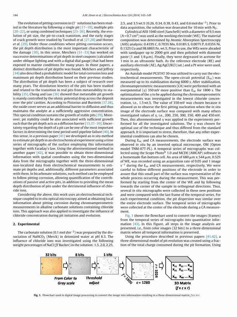
Fig. 1 shows the flowchart used to convert the images (frames)from the temporal series of micrographs into quantitative infor-mation [43]. In this Figure, all steps in the image analysis arepresented, i.e., from color images (32 bits) to a three-dimensional

matrix where all temporal information is preserved.

Using the procedure described in previous papers [41,42], athree-dimensional model of pit evolution was created using a frac-tion of the total charge consumed during the pit formation. Using

into information resulting in a three-dimensional matrix, f x c x r.

A.M. Zimer et al. / Electrochimica Acta 124 (2014) 143–149 145

Ft

Fttttitp

3

tdlo(cF

lmopIT2w

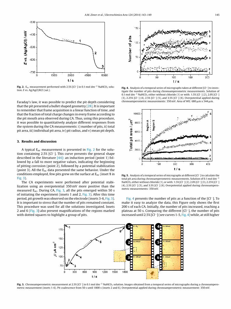
Fig. 4. Analysis of a temporal series of micrographs taken at different [Cl−] to inves-tigate the number of pits during chronoamperometric measurements. Solution of0.1 mol dm−3 NaHCO3 either without chloride (1) or with: 1.5% [Cl−] (2), 2.0% [Cl−](3), 2.25% [Cl−] (4), 2.5% [Cl−] (5), and 3.5% [Cl−] (6). Overpotential applied duringchronoamperometric measurements: 350 mV. Area of WE: 680 �m x 544 �m.

Fig. 5. Analysis of a temporal series of micrographs at different [Cl−] to calculate thetotal pit area during chronoamperometric measurements. Solution of 0.1 mol dm−3

− − −

make it easy to analyze the data, this Figure only shows the first

Fm

ig. 2. Eoc measurement performed with 2.5% [Cl−] in 0.1 mol dm−3 NaHCO3 solu-ion. E vs. Ag/AgCl/KCl (sat.).

araday’s law, it was possible to predict the pit depth consideringhat the pit presented a bullet shaped geometry [28]. It is importanto remember that frame acquisition is a linear function of time, andhat the fraction of total charge changes in every frame according tohe pit mouth area observed during CA. Thus, using this procedure,t was possible to quantitatively analyze different responses fromhe system during the CA measurements: i) number of pits, ii) totalit area, iii) individual pit area, iv) pit radius, and v) mean pit depth.

. Results and discussion

A typical Eoc measurement is presented in Fig. 2 for the solu-ion containing 2.5% [Cl−]. This curve presents the general shapeescribed in the literature [44]: an induction period (point 1) fol-

owed by a fall to more negative values, indicating the beginningf pitting corrosion (point 2), followed by a potential stabilizationpoint 3). All the Eoc data presented the same behavior. Under theonditions employed, few pits grew on the surface at Eoc (inset 1 inig. 3).

The CA experiments were performed after potential stabi-ization using an overpotential 350 mV more positive than the

easured Eoc. During CA, Fig. 3, all the pits emerged within 50 sf initiating the experiment (insets 1 and 2, Fig. 3). After this timeeriod, pit growth was observed on the electrode (insets 3-6, Fig. 3).

t is important to stress that the number of pits remained constant.

his procedure was used for all the solutions investigated. Insets

and 6 (Fig. 3) also present magnifications of the regions markedith dotted squares to highlight a group of pits.

ig. 3. Chronoamperometric measurement at 2.5% [Cl−] in 0.1 mol dm−3 NaHCO3 solutioetric measurement (insets 1-6). Pit coalescence from 50 s until 1800 s (insets 2 and 6).

NaHCO3 either without chloride (1), or with: 1.5% [Cl ] (2), 2.0% [Cl ] (3), 2.25% [Cl ](4), 2.5% [Cl−] (5), and 3.5% [Cl−] (6). Overpotential applied during chronoampero-metric measurements: 350 mV.

Fig. 4 presents the number of pits as a function of the [Cl−]. To

200 s of each CA. Initially, the number of pits increased, reaching aplateau at 50 s. Comparing the different [Cl−], the number of pitsincreased until 2.5% [Cl−] (see curves 1-5, Fig. 4) while, at still higher

n. Images obtained from a temporal series of micrographs during a chronoampero-Overpotential applied during chronoamperometric measurement: 350 mV.

146 A.M. Zimer et al. / Electrochimica Acta 124 (2014) 143–149

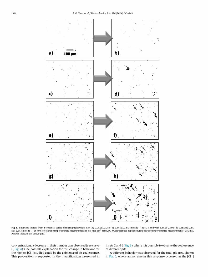
Fig. 6. Binarized images from a temporal series of micrographs with: 1.5% (a), 2.0% (c), 2.25% (e), 2.5% (g), 3.5% chloride (i) at 50 s, and with 1.5% (b), 2.0% (d), 2.25% (f), 2.5%( 3 NaHA

c6tT

h), 3.5% chloride (j) at 400 s of chronoamperometric measurement in 0.1 mol dmrrows indicate the active pits.

oncentrations, a decrease in their number was observed (see curve, Fig. 4). One possible explanation for this change in behavior forhe highest [Cl−] studied could be the existence of pit coalescence.his proposition is supported in the magnifications presented in

CO3. Overpotential applied during chronoamperometric measurements: 350 mV.

insets 2 and 6 (Fig. 3), where it is possible to observe the coalescenceof different pits.

A different behavior was observed for the total pit area, shownin Fig. 5, where an increase in this response occurred as the [Cl−]

A.M. Zimer et al. / Electrochimica Acta 124 (2014) 143–149 147

Table 1Total pit area changes in Region A (0–50 s) and in Region B (100–400 s) during theCA experiment presented in Fig.5.

[Cl−] (wt.%) Total pit area changes/�m2 s−1

A (0–50 s) B (100–400 s)

1.5 3.3 ± 0.6 0.10 ± 0.032.0 19.5 ± 1.0 1.6 ± 0.04

iv5fgtt

roTpd(

tfFtnrp2ctt[ws

pt

Fsc33

Fig. 8. Pit radius analysis for 10 pits during a chronoamperometric measurementin 2.25% [Cl−]. The dotted lines indicate the active pits that grew continuously and

2.25 66.0 ± 2.9 5.7 ± 0.102.5 84.1 ± 4.3 6.8 ± 0.183.5 70.5 ± 2.2 13.8 ± 0.23

ncreased. Otherwise, for each solution, a tendency to a constantalue was observed when the polarization time was greater than0 s, except for the 3.5% [Cl−] solution. One possible explanationor this behavior is that, after 50 s, only a few pits continued torow. Then the total pit area remained approximately constanthroughout the experimental run. This hypothesis will be inves-igated further in the following text.

As discussed above, Fig. 5 can be divided into two distinctegions, indicated by a dotted line in that Figure. The first, region A,ccurs up until 50 s, where the pit area presents a sharp increase.he second, region B, occurs after this time, during which the totalit area shows only a slow increase. In order to summarize theseata, the slopes of these curves were calculated in each regionTable 1).

From the results presented in Table 1, it is possible to observehat the first slope increased for [Cl−] up to 2.5% but then decreasedor [Cl−] at 3.5%. These results are similar to those highlighted inig. 4, where for [Cl−] greater than 2.5% there was a decrease inhe number of pits compared to lower [Cl−]. One possible expla-ation for this fact is the coexistence of two phenomena in thisegion, such as new pit nucleation and pit growth. In other words,it nucleation could govern the changes observed in slope A until.5% [Cl−] (see Fig. 4). On the other hand, in the second region, thehanges observed in slope B are only affected by pit growth oncehe number of pits is constant (see also Fig. 4). Thus, an increase inhe number of active pits must be observed on the metal surface asCl−] increases. This proposition can easily be confirmed in Fig. 6,here the arrows indicate those pits that continue to grow from 50

to 400 s.This complex behavior is also observed in Fig. 7, where the mean

it radius (rmean) as a function of the time is plotted for all the inves-igated solutions. In this Figure, it can be observed that until 50 s,

ig. 7. Mean pit radius analysis for all pits during the chronoamperometric mea-urements at all [Cl−] investigated. Solution of 0.1 mol dm−3 NaHCO3 either withouthloride (1), or with: 1.5% [Cl−] (2), 2.0% [Cl−] (3), 2.25% [Cl−] (4), 2.5% [Cl−] (5), and.5% [Cl−] (6). Overpotential applied during chronoamperometric measurements:50 mV.

straight lines indicate passivated pits that ceased to grow at 50 s. Solution of 0.1 moldm−3 NaHCO3. Overpotential applied during chronoamperometric measurement:350 mV.

there was a strong increase in rmean values, which could be asso-ciated with pit growth on the surface after nucleation. After thistime point, an evident decrease in this parameter was observed,which could be attributed to the formation of protective FeCO3scales inside the pits, although some of them still continue to grow.This last proposition can also be clearly observed in Fig. 6.

A second argument to test the latter statement is the behaviorverified for several individual pits, which are presented in Fig. 8.This Figure presents an experiment performed in 2.25% [Cl−], whichis representative of the general behavior observed in all otherstudied solutions. As can be observed, some of the pit radii grewcontinuously while others clearly stopped changing, characteris-tic of passive and active pits, respectively [37]. In this case, a pitstabilization criterion must be reached during pit growth to avoidrepassivation [36]. In the corrosion of carbon steel by CO2, the exist-ence of active pits could be related to the precipitation of FeCO3inside them, which induces local acidification as described in theliterature [1,11]. Therefore, a subsequent increase in [Cl−] occursto counterbalance the H+ ions produced [11]. Then, the existenceof mass transport through the scale inside the pit could determinetheir activity or passivity [1]. Another point that can sustain thegrowth of active pits is the behavior of pit depth [15,37,38], whichis described in the following paragraphs.

It is important to point out that the interpretation of Fig. 8 cor-roborates the total pit area behavior presented in Fig. 5, i.e., wheretwo distinct regions were found. As proposed above, pit nuclea-tion probably governs the changes observed in region A, while pitgrowth governs the changes in region B (Fig. 5 and Table 1). Then,considering all the data combined, most probably the existence ofthe second slope observed in Fig. 5 is related to the presence ofa small number of active pits that are still growing in region B.Therefore, in region B, only these active pits are responsible forthe observed behavior. These results are in qualitative agreementwith those described by Melchers and Jeffrey [34], who found adistinct depth distribution during pit corrosion of steel coupons ina marine environment. Here, a distinct radii distribution was alsoobserved once active and passive pits were detected on the metalsurface.

In this context, Fig. 9 presents the mean pit depth (Lpit) behav-ior, calculated using a procedure described previously [41,42]. This

model is based on the fraction of the charge for each pit at each timepoint during electrochemical experiments. Then the pit volume(Vpit) is calculated using Faraday’s law, considering a bullet-shapedpit to estimate the pit depth (Lpit). As can be observed in Fig. 9,

148 A.M. Zimer et al. / Electrochimica

Fig. 9. Mean pit depth during the chronoamperometric measurement at all [Cl−]i −3

[a

fiarFt(

ptmo

tamu

4

rtsiNtci[fiaierfFt

A

C

[

[

[

[

[

[

[

[

[

[

[

[

[

[

[

[

[

[

[

[

[

nvestigated. Solution of 0.1 mol dm NaHCO3 without chloride (1), or with: 1.5%Cl−] (2), 2.0% [Cl−] (3), 2.25% [Cl−] (4), 2.5% [Cl−] (5), and 3.5% [Cl−] (6). Overpotentialpplied during chronoamperometric measurements: 350 mV.

or [Cl−] greater than 2.5%, there is a change in the Lpit behav-or. According to Pistorius and Burstein [37,38], pit stability couldlso be associated with pit depth, which acts as a diffusion bar-ier to sustain stable pit growth. This affirmation is corroborated inig. 9 along with the in situ binarized images of Fig. 6 (see arrows)hat show a high occurrence of active pits in the same experimentFig. 6f).

Further work based on temporal series of micrographs cou-led with electrochemical techniques [41,42] could also be doneo obtain the individual depth of each pit. This would require some

odifications to the model described in the previous paragraph inrder to estimate the depth of each pit.

In summary, the approach used here allows different parame-ers associated with pits to be followed as a function of time duringn electrochemical experiment. In this sense, substantial infor-ation can be provided, which immensely contributes to overall

nderstanding of the pit growth mechanism.

. Conclusions

This study presents a method to study corrosion reactions ineal time by analyzing a temporal series of micrographs coupledo electrochemical techniques. During chronoamperometric mea-urements, it was observed that the number of pits increasednitially and then stabilized at a plateau value at all the [Cl−] studied.evertheless, a different behavior was observed for [Cl−] greater

han 2.5%, where a decrease in the number of pits was foundompared to experiments at lower [Cl−]. Otherwise, a monotonicncrement in the total pit area was found that was proportional toCl−]. From this last plot, two slopes were calculated where, for therst one, region A, both pit nucleation and growth were observednd there was evidence that pit nucleation governs the processn this region. The pit radius analysis allowed us to infer the exist-nce of two different kinds of pits, i.e. active and passive. Therefore,egion B is governed by the growth of active pits in the metal sur-ace. Finally, based on the fraction of the total charge and usingaraday’s law, it was possible to estimate the mean pit depth onhe metal surface during the progress of pitting corrosion.

cknowledgments

The authors would like to thank FAPESP (process 11/19430-0),NPq and CAPES for their financial support.

[

[

Acta 124 (2014) 143–149

References

[1] S. Nesic, Key issues related to modelling of internal corrosion of oil and gaspipelines–A review, Corros. Sci. 49 (2007) 4308–4338.

[2] S. Nesic, Effects of Multiphase Flow on Internal CO2 Corrosion of Mild SteelPipelines, Energy & Fuels 26 (2012) 4098–4111.

[3] Z.F. Yin, W.Z. Zhao, Z.Q. Bai, Y.R. Feng, W.J. Zhou, Corrosion behavior of SM 80SStube steel in stimulant solution containing H2S and CO2, Electrochim. Acta 53(2008) 3690–3700.

[4] S. Mattar, L.F. Hatch, Chemistry of Petrochemical Processes, 2nd Ed., EUA, 2000.[5] G.A. Zhang, Y. Zeng, X.P. Guo, F. Jiang, D.Y. Shi, Z.Y. Chen, Electrochemical

corrosion behavior of carbon steel under dynamic high pressure H2S/CO2 envi-ronment, Corros. Sci. 65 (2012) 37–47.

[6] P. Altoé, G. Pimenta, C.F. Moulin, S.L. Díaz, O.R. Mattos, Evaluation of oilfieldcorrosion inhibitors CO2 containing media: A kinetic study, Electrochem. Acta41 (1996) 1165–1172.

[7] F. Fayez, E. Mahdi, A. Alfantazi, Electrochemical evaluation of the corrosionbehaviour of API-X100 pipeline steel in aerated bicarbonate solutions, Corros.Sci. 58 (2012) 181–191.

[8] P. Refait, M. Abdelmoula, J.R. Génin, R. Sabot, Green rusts in electrochemi-cal and microbially influenced corrosion of steel, C. R. Geoscience 338 (2006)476–487.

[9] V. Ruzic, M. Veidt, S. Nesic, Protective iron carbonate films - Part 2: Chemi-cal removal by dissolution in single-phase aqueous flow, Corrosion 62 (2006)598–611.

10] K.S. George, S. Nesic, Investigation of carbon dioxide corrosion of mild steel inthe presence of acetic acid — Part 1: Basic mechanisms, Corros. Sci. 63 (2007)178–186.

11] M. Reffass, R. Sabot, M. Jeannin, C. Berziou, P. Refait, Effects of phosphate specieson localised corrosion of steel in NaHCO3 + NaCl electrolytes, Electrochim. Acta54 (2009) 4389–4396.

12] M. Reffass, R. Sabot, C. Savall, M. Jeannin, J. Creus, P. Refait, Localised corrosion ofcarbon steel in NaHCO3/NaCl electrolytes: role of Fe(II)-containing compounds,Corros. Sci. 48 (2006) 709–726.

13] Y.F. Cheng, M. Wilmott, J.L. Luo, The role of chloride ions in pitting of carbonsteel studied by the statistical analysis of electrochemical noise, Appl. Surf. Sci.152 (1999) 161–168.

14] P. Marcus, V. Maurice, H.-. Strehblow, Localized corrosion (pitting): A modelof passivity breakdown including the role of the oxide layer nanostructure,Corros. Sci. 50 (2008) 2698–2704.

15] G.S. Frankel, Pitting Corrosion of Metals: A Review of the Critical Factors, J.Electrochem. Soc. 145 (1998) 2186–2198.

16] M.A. Amin, Passivity and passivity breakdown of a zinc electrode in aeratedneutral sodium nitrate solutions, Electrochim. Acta 50 (2005) 1265–1274.

17] R.C. Alkire, K.P. Wong, The corrosion of single pits on stainless steel in acidchloride solution, Corros. Sci. 28 (1988) 411–421.

18] J.O. Park, M. Verhoff, R. Alkire, Microscopic behavior of single corrosion pits:the effect of thiosulfate on corrosion of stainless steel in NaCl, Electrochim. Acta42 (1997) 3281–3291.

19] N.J. Laycock, S.P. White, Computer simulation of single pit propagation instainless steel under potentiostatic control, J.Electrochem Soc. 148 (2001)B264–B275.

20] R.E. Melchers, Discussion on Stochastic modeling of pitting corrosion: A newmodel for initiation and growth of multiple pits by A. Valor, F., Caleyo, L.,Alfonso, D., Rivas, J.M. Hallen [Corros. Sci. 49 (2007) 559], Corrosion 50 (2008)1518–1519.

21] R.E. Melchers, Extreme value statistics and long-term marine pitting corrosionof steel, Probabilist. Eng. Mech. 23 (2008) 482–488.

22] I.A. Chaves, R.E. Melchers, Pitting corrosion in pipeline steel weld zones, Corros.Sci. 53 (2011) 4026–4032.

23] H. Böhni, T. Suter, A. Schreyer, Micro- and nanotechniques to study localizedcorrosion, Electrochim. Acta 40 (1995) 1361–1368.

24] C. Punckt, M. Bölscher, H.H. Rotermund, A.S. Mikhailov, L. Organ, N. Budian-sky, et al., Sudden onset of pitting corrosion on stainless steel as a criticalphenomenon, Science 305 (2004) 1133–1136.

25] V. Vignal, H. Krawiec, O. Heintz, R. Oltra, The use of local electrochemical probesand surface analysis methods to study the electrochemical behaviour and pit-ting corrosion of stainless steels, Electrochim. Acta 52 (2007) 4994–5001.

26] S.M. Ghahari, A.J. Davenport, T. Rayment, T. Suter, J. Tinnes, C. Padovani, et al.,In situ synchrotron X-ray micro-tomography study of pitting corrosion in stain-less steel, Corros. Sci. 53 (2011) 2684–2687.

27] A. Turnbull, L.N. McCartney, S. Zhou, A model to predict the evolution of pittingcorrosion and the pit-to-crack transition incorporating statistically distributedinput parameters, Corros. Sci. 48 (2006) 2084–2105.

28] A. Turnbull, D.A. Horner, B.J. Connolly, Challenges in modelling the evolutionof stress corrosion cracks from pits, Eng. Fract. Mech. 76 (2009) 633–640.

29] D.A. Horner, B.J. Connolly, S. Zhou, L. Crocker, A. Turnbull, Novel images of theevolution of stress corrosion cracks from corrosion pits, Corros. Sci. 53 (2011)3466–3485.

30] A. Jarrah, M. Bigerelle, G. Guillemot, D. Najjar, A. Iost, J.-. Nianga, A generic sta-tistical methodology to predict the maximum pit depth of a localized corrosion

process, Corros.Sci. 53 (2011) 2453–2467.

31] R.E. Melchers, Statistical characterization of pitting corrosion - Part 1: Dataanalysis, Corrosion 61 (2005) 655–664.

32] R.E. Melchers, Statistical characterization of pitting corrosion - Part 2: Proba-bilistic modeling for maximum pit depth, Corrosion 61 (2005) 766–777.

imica

[

[

[

[

[

[

[

[

[

[

[

A.M. Zimer et al. / Electroch

33] R.E. Melchers, Pitting corrosion of mild steel in marine immersion environment- Part 1: Maximum pit depth, Corrosion 60 (2004) 824–836.

34] R.E. Melchers, R.J. Jeffrey, Probabilistic models for steel corrosion loss and pit-ting of marine infrastructure, Reliab. Eng. Syst. Safe. 93 (2008) 423–432.

35] N.J. Laycock, R.C. Newman, Localised dissolution kinetics, salt films and pittingpotentials, Corros. Sci. 39 (1997) 1771–1790.

36] Y.F. Cheng, J.L. Luo, Passivity and pitting of carbon steel in chromate solutions,Electrochim. Acta 44 (1999) 4795–4804.

37] P.C. Pistorius, G.T. Burstein, Growth of corrosion pits on stainless steel in chlo-ride solution containing dilute sulphate, Corros. Sci. 33 (1992) 1885–1897.

38] P.C. Pistorius, G.T. Burstein, Aspects of the effects of electrolyte composition onthe occurrence of metastable pitting on stainless steel, Corros. Sci. 36 (1994)525–538.

39] P. Ernst, R.C. Newman, Pit growth studies in stainless steel foils. I. Introductionand pit growth kinetics, Corros. Sci. 44 (2002) 927–941.

[

Acta 124 (2014) 143–149 149

40] J.E. Strutt, J.R. Nicholls, B. Barbier, The prediction of corrosion by statisticalanalysis of corrosion profiles, Corros. Sci. 25 (1985) 305–315.

41] A.M. Zimer, E.C. Rios, L.H. Mascaro, E.C. Pereira, Temporal series micrographscoupled with polarization curves to study pit corrosion, Electrochem. Com-mum. 13 (2011) 1484–1487.

42] A.M. Zimer, M.A. Carra, E.C. Rios, E.C. Pereira, L.H. Mascaro, Initial stages ofcorrosion pits on AISI 1040 steel in sulfide solution analyzed by temporal seriesmicrographs coupled with electrochemical techniques, Corros. Sci. 76 (2013)27–34.

43] A.M. Zimer, E.C. Rios, P.D. Mendes, W.N. Gonc alves, O.M. Bruno, E.C. Pereira,

et al., Investigation of AISI 1040 steel corrosion in H2S solution containing chlo-ride ions by digital image processing coupled with electrochemical techniques,Corros. Sci. 53 (2011) 3193–3201.

44] A.D. Davydov, Analysis of pitting corrosion rate, Russ. J. Electrochem. 44 (2007)835–839.